跳到论文正文
W Papers独立论文阅读器 arXiv:1303.4848 论文正文 计算阅读时间 · 0%
引用这篇论文根据当前论文元数据生成,正式投稿前建议核对。


License: arXiv.org perpetual non-exclusive license
arXiv:1303.4848v2 [hep-ph] 10 May 2013

Unitarity and vacuum stability constraints on the couplings of color octet scalars

Xiao-Gang He1,2,3 Note: hexg@phys.ntu.edu.tw Affiliation: 1Physics Division, National Center for Theoretical Sciences,
Department of Physics, National Tsing Hua University, Hsinchu, Taiwan
   Han Phoon4 Note: hphoon@iastate.edu Affiliation: 1Physics Division, National Center for Theoretical Sciences,
Department of Physics, National Tsing Hua University, Hsinchu, Taiwan
   Yong Tang1 Note: ytang@phys.cts.nthu.edu.tw Affiliation: 1Physics Division, National Center for Theoretical Sciences,
Department of Physics, National Tsing Hua University, Hsinchu, Taiwan
   German Valencia4 Note: valencia@iastate.edu Affiliation: 1Physics Division, National Center for Theoretical Sciences,
Department of Physics, National Tsing Hua University, Hsinchu, Taiwan
Affiliation: 2INPAC, Department of Physics, Shanghai Jiao Tong University, Shanghai, China Affiliation: 3CTS, CASTS and Department of Physics, National Taiwan University, Taipei, Taiwan Affiliation: 4Department of Physics, Iowa State University, Ames, IA 50011, United States
August 24, 2026
Abstract

The recent discovery of a 126 GeV boson at the LHC will be followed by a detailed examination of its couplings in order to determine whether this particle is the Higgs boson of the standard model or one of many particles of an extended scalar sector. One such extension with a rich phenomenology consists of a color octet electroweak doublet scalar. The most general renormalizable scalar potential contains twelve new parameters and it is therefore desirable to constrain them. We present theoretical constraints on these parameters obtained by requiring perturbative unitarity for two-to-two scalar scattering amplitudes at high energy and vacuum stability.

pacs
PACS numbers:

I Introduction

The two experiments ATLAS and CMS at the Large Hadron Collider (LHC) have found a new resonant state of mass near 126 GeV [1, 2]. The properties of this state that have been tested so far match those expected for the standard model, but much work remains to be done to confirm that this is indeed the SM Higgs hh. Many interesting possibilities for new physics remain open at this point. By measuring the coupling strengths of the new state to the known standard model bosons and fermions the experiments should be able to unravel the nature of the new state.

New physics possibilities remain open even if this new state is the SM Higgs boson because the value of its mass suggests that the vacuum may not be completely stable [3, 4, 5, 6, 7]. In the SM, vacuum stability is closely related to the physical Higgs mass mhm_{h} since the quartic self-coupling λ\lambda in the Higgs potential is related to it by λ=mh/2​v\lambda=m_{h}/\sqrt{2}\ v (v=246v=246 GeV). This quartic coupling must remain positive to guarantee that the Higgs potential is bounded from below. In the SM the top quark contribution to radiative corrections can drive λ\lambda negative, induce a false and deep minimum at large field values and destabilize the electroweak vacuum. In the SM with a Higgs mass near 126 GeV, the turning point is at an energy scale of order 101010^{10} GeV and there is no immediate conflict with data. However, if we require the vacuum to be stable up to grand unification or even Planck scales, new physics is required to change the running of λ\lambda[8, 9, 10, 11, 12, 13, 14, 15, 16, 17, 18, 19, 20, 21]. In general this new physics will also affect the phenomenology of Higgs production and decay at the LHC.

In this paper we consider a simple extension of the scalar sector of the SM with new scalars SS transforming as (8,2,1/2)(8,2,1/2) under the SM gauge group S​U​(3)C×S​U​(2)L×U​(1)YSU(3)_{C}\times SU(2)_{L}\times U(1)_{Y}. This color octet, electroweak doublet, scalar extension of the SM is motivated by the requirement of minimal flavor violation [22, 23, 24]. The most general renormalizable scalar potential for this model contains twelve new parameters and it is therefore desirable to constrain them. We compute theoretical constraints on these parameters by requiring perturbative unitarity for the two-to-two scalar scattering amplitudes at high energy, as well as by requiring vacuum stability in the form of a positive λ\lambda.

In addition to the color octet, the scalar sector of this model contains a Higgs boson from the doublet H:(1,2,1/2)H:(1,2,1/2) which is responsible for spontaneous electroweak symmetry breaking and has the same tree level couplings as the SM hh to other SM particles. The additional colored scalars are assumed to be heavier and the phenomenology related to their possible observation at LHC has been studied before. The new scalars can induce important loop effects which are substantially different from the SM due to new parameters in the Yukawa and Higgs potential sectors. We will discuss the effects of this extension of the SM on the question of vacuum stability and we will address the phenomenology of the loop level Higgs couplings h​g​ghgg and h​γ​γh\gamma\gamma in a separate publication [25].

II The model

The model we consider is an extension of the scalar sector of the SM to which a color octet, electroweak doublet of scalars is added. The inclusion of the new multiplet SS introduces several new, renormalizable, interaction terms to the Lagrangian. Because SS has non-trivial S​U​(3)C×S​U​(2)L×U​(1)YSU(3)_{C}\times SU(2)_{L}\times U(1)_{Y} quantum numbers, it will have corresponding gauge interactions. In addition there will be new terms in the Yukawa couplings and in the Higgs potential that are consistent with minimal flavor violation. Following Ref. [24] we write the Yukawa couplings as

ℒY=−η~U​gi​jU​u¯R​i​TA​Qj​SA−η~D​gi​jD​d¯R​i​TA​Qj​S†A+h.c,\mathcal{L}_{Y}=-\tilde{\eta}_{U}g^{U}_{ij}\bar{u}_{Ri}T^{A}Q_{j}S^{A}-\tilde{\eta}_{D}g^{D}_{ij}\bar{d}_{Ri}T^{A}Q_{j}S^{\dagger A}+h.c, (1)

where QiQ_{i} are left-handed quark doublets, S=Sa​Ta​(a=1,…,8)S=S^{a}T^{a}\;(a=1,...,8) with the S​U​(3)SU(3) generators normalized as Tr​(Ta​Tb)=δa​b/2\textrm{Tr}(T^{a}T^{b})=\delta^{ab}/2. The matrices gi​jU,Dg^{U,D}_{ij} are the same as those coupling the Higgs to quarks, and ηU,D\eta_{U,D} are new overall factors that can be complex. In the quark mass eigenstate basis these couplings are given by

ℒ\displaystyle{\cal L} =\displaystyle= −2v​η~U​U¯R​Ta​M^u​UL​Sa​0+2v​η~U​U¯R​Ta​M^u​VK​M​DL​Sa+\displaystyle-{\sqrt{2}\over v}\tilde{\eta}_{U}\bar{U}_{R}T^{a}\hat{M}^{u}U_{L}S^{a0}+{\sqrt{2}\over v}\tilde{\eta}_{U}\bar{U}_{R}T^{a}\hat{M}^{u}V_{KM}D_{L}S^{a+} (2)
−\displaystyle- 2vη~DD¯RTaM^dDLSa0†−2vη~DD¯RTaM^uV†K​MULSa−+h.c.,\displaystyle{\sqrt{2}\over v}\tilde{\eta}_{D}\bar{D}_{R}T^{a}\hat{M}^{d}D_{L}S^{a0\dagger}-{\sqrt{2}\over v}\tilde{\eta}_{D}\bar{D}_{R}T^{a}\hat{M}^{u}V^{\dagger}_{KM}U_{L}S^{a-}+{\rm~h.c.},

where M^u,d\hat{M}^{u,d} are the diagonal quark mass matrices, M^u,d=diag⁡(mu,d,mc,s,mt,b)\hat{M}^{u,d}={\rm diag}(m_{u,d},m_{c,s},m_{t,b}); the quark fields are UL,R=diag⁡(uL,R,cL,R,tL,R)U_{L,R}={\rm diag}(u_{L,R},c_{L,R},t_{L,R}) and DL,R=diag⁡(dL,R,sL,R,bL,B)D_{L,R}={\rm diag}(d_{L,R},s_{L,R},b_{L,B}). The neutral complex field Sa​0S^{a0} can be further decomposed into a scalar SRa​0S^{a0}_{R} and a pseudo-scalar SIa​0S^{a0}_{I} as Sa​0=(SRa​0+i​SIa​0)/2S^{a0}=(S^{a0}_{R}+i\ S^{a0}_{I})/\sqrt{2}. The parameters η~U,D\tilde{\eta}_{U,D} are expected to be of order one and are in general complex. We will write them as η~U,D=ηU,D​ei​αu,d\tilde{\eta}_{U,D}=\eta_{U,D}e^{i\alpha_{u,d}} with ηU,D\eta_{U,D} real, and if there are non-zero phases αu,d\alpha_{u,d} there is C​PCP violation beyond the SM.

The most general renormalizable scalar potential is given in Ref. [24] as11 1 We use a normalization of λ\lambda different than Ref. [24] in order to have the conventional relation λ=GF​mH2/2\lambda=G_{F}m_{H}^{2}/\sqrt{2}.

V\displaystyle V =\displaystyle= λ​(H†i​Hi−v22)2+2​ms2​Tr​S†i​Si+λ1​H†i​Hi​Tr​S†j​Sj+λ2​H†i​Hj​Tr​S†j​Si\displaystyle\lambda\left(H^{\dagger i}H_{i}-\frac{v^{2}}{2}\right)^{2}+2m_{s}^{2}\ {\rm Tr}S^{\dagger i}S_{i}+\lambda_{1}\ H^{\dagger i}H_{i}\ {\rm Tr}S^{\dagger j}S_{j}+\lambda_{2}\ H^{\dagger i}H_{j}\ {\rm Tr}S^{\dagger j}S_{i} (3)
+\displaystyle+ (λ3H†iH†jTrSiSj+λ4ei​ϕ4H†iTrS†jSjSi+λ5ei​ϕ5H†iTrS†jSiSj+H.c.)\displaystyle\left(\lambda_{3}\ H^{\dagger i}H^{\dagger j}\ {\rm Tr}S_{i}S_{j}+\lambda_{4}\ e^{i\phi_{4}}\ H^{\dagger i}{\rm Tr}S^{\dagger j}S_{j}S_{i}+\lambda_{5}\ e^{i\phi_{5}}\ H^{\dagger i}{\rm Tr}S^{\dagger j}S_{i}S_{j}+{\rm~H.c.}\right)
+\displaystyle+ λ6​Tr​S†i​Si​S†j​Sj+λ7​Tr​S†i​Sj​S†j​Si+λ8​Tr​S†i​Si​Tr​S†j​Sj\displaystyle\lambda_{6}\ {\rm Tr}S^{\dagger i}S_{i}S^{\dagger j}S_{j}+\ \lambda_{7}\ {\rm Tr}S^{\dagger i}S_{j}S^{\dagger j}S_{i}+\ \lambda_{8}\ {\rm Tr}S^{\dagger i}S_{i}\ {\rm Tr}S^{\dagger j}S_{j}
+\displaystyle+ λ9​Tr​S†i​Sj​Tr​S†j​Si+λ10​Tr​Si​Sj​Tr​S†i​S†j+λ11​Tr​Si​Sj​S†j​S†i.\displaystyle\lambda_{9}\ {\rm Tr}S^{\dagger i}S_{j}\ {\rm Tr}S^{\dagger j}S_{i}+\ \lambda_{10}\ {\rm Tr}S_{i}S_{j}\ {\rm Tr}S^{\dagger i}S^{\dagger j}+\ \lambda_{11}\ {\rm Tr}S_{i}S_{j}S^{\dagger j}S^{\dagger i}.

Here v∼246v\sim 246 GeV is the Higgs vacuum expectation value (vev) with ⟨H⟩=v/2\langle H\rangle=v/\sqrt{2}. The traces are over the color indices and the S​U​(2)SU(2) indices i,ji,j are displayed explicitly. We follow Ref. [24] to pick a real λ3\lambda_{3} by a suitable definition of SS fields and have displayed the two possible phases ϕ4,5\phi_{4,5} explicitly, all the λ′​s\lambda^{\prime}s in Eq. 3 are thus real.

Although implementation of minimal flavor violation reduces the parameters in the Yukawa sector, there are still a large number of parameters in the scalar potential VV. These parameters have physical effects and are constrained from various theoretical and experimental considerations. In order to have an unbroken color symmetry, the parameters must be chosen such that SS cannot develop a non-zero vev, but HH must have the usual non-zero vev to induce electroweak symmetry breaking. In order for the potential to be bounded from below λ\lambda must be larger than zero and several of λi\lambda_{i}s must be positive. Maintaining unitarity of the scattering amplitudes induced by the new parameters also constrains them.

After symmetry breaking, the non-zero vev of the Higgs gives the physical Higgs scalar hh a mass mH2=2​λ​v2m^{2}_{H}=2\lambda v^{2} and it also splits the octet scalar masses. The resulting tree level mass spectrum for the colored scalars is [24]

mS±2\displaystyle m^{2}_{S^{\pm}} =\displaystyle= mS2+λ1​v24,\displaystyle m^{2}_{S}+\lambda_{1}\frac{v^{2}}{4},
mSR02\displaystyle m^{2}_{S^{0}_{R}} =\displaystyle= mS2+(λ1+λ2+2​λ3)​v24,\displaystyle m^{2}_{S}+\left(\lambda_{1}+\lambda_{2}+2\lambda_{3}\right)\frac{v^{2}}{4}, (4)
mSI02\displaystyle m^{2}_{S^{0}_{I}} =\displaystyle= mS2+(λ1+λ2−2​λ3)​v24,\displaystyle m^{2}_{S}+\left(\lambda_{1}+\lambda_{2}-2\lambda_{3}\right)\frac{v^{2}}{4},

The parameters mS2m_{S}^{2}, and λ1,2,3\lambda_{1,2,3} should be chosen such that the above masses remain positive. When not stated explicitly, we shall denote the colored scalar masses collectively by MSM_{S}.

It has been noted that Eq. 3 respects the custodial S​U​(2)SU(2) symmetry of the SM model if [24, 26, 27]

2​λ3=λ2, 2​λ6=2​λ7=λ11,λ9=λ10,λ4=λ5⋆.\displaystyle 2\lambda_{3}=\lambda_{2},\,2\lambda_{6}=2\lambda_{7}=\lambda_{11},\,\lambda_{9}=\lambda_{10},\,\lambda_{4}=\lambda_{5}^{\star}. (5)

When these conditions are imposed, constraints from the TT parameter, from electroweak precision data, are automatically satisfied.

III Two-to-two scalar scattering amplitudes and unitarity constraints

In this section we consider high energy two-to-two scalar scattering to constrain the strength of the self interactions with the requirement of perturbative unitarity. Although the potential is renormalizable, the tree-level scattering amplitudes approach a constant at high energy that is proportional to the quartic couplings. Perturbative unitarity then constrains their size in a manner entirely analogous to the unitarity bound on the SM Higgs boson mass [28] and generalizations [29]. We will consider scattering of all the scalar particles that appear in the model at energies much larger than their masses. In this limit, the Higgs and the SM would be Goldstone bosons can be treated as degenerate and massless, and the colored scalars as degenerate with mass mSm_{S}. The strongest limits on the couplings are obtained by considering scattering of two particle states of definite color and I=0I=0. In this context, I=0I=0 is the singlet of the approximate O⁡(4)O(4) symmetry between H,w±,zH,w^{\pm},z (referred collectively as hh) and between S±,Si,SrS^{\pm},S_{i},S_{r}. The normalization of the two particle states will then be

|S​S⟩0\displaystyle|SS\rangle_{0} ≡\displaystyle\equiv 18​Sa​Sa\displaystyle\frac{1}{\sqrt{8}}S^{a}S^{a}
|S​S⟩8​S\displaystyle|SS\rangle_{8S} ≡\displaystyle\equiv 35​da​b​c​Sa​Sb\displaystyle\sqrt{\frac{3}{5}}d_{abc}S^{a}S^{b}
|S​S⟩8​A\displaystyle|SS\rangle_{8A} ≡\displaystyle\equiv 13​fa​b​c​Sa​Sb,\displaystyle\frac{1}{\sqrt{3}}f_{abc}S^{a}S^{b}, (6)

for the color singlet, the symmetric octet and the antisymmetric octet respectively. The I=0I=0 two particle state will be

|h​h⟩I=0\displaystyle|hh\rangle_{I=0} ≡\displaystyle\equiv 18​(w+​w−+w−​w++z​z+h​h)\displaystyle\frac{1}{\sqrt{8}}(w^{+}w^{-}+w^{-}w^{+}+zz+hh)
|S​S⟩I=0\displaystyle|SS\rangle_{I=0} ≡\displaystyle\equiv 18​(Sa+​Sb−+Sa−​Sb++Sia​Sib+Sra​Srb)\displaystyle\frac{1}{\sqrt{8}}(S^{a+}S^{b-}+S^{a-}S^{b+}+S_{i}^{a}S_{i}^{b}+S_{r}^{a}S_{r}^{b})
|h​S⟩I=0\displaystyle|hS\rangle_{I=0} ≡\displaystyle\equiv 18​(w+​Sc−+w−​Sc++Sic​z+Src​h)\displaystyle\frac{1}{\sqrt{8}}(w^{+}S^{c-}+w^{-}S^{c+}+S_{i}^{c}z+S_{r}^{c}h) (7)

for two color singlet scalars, two color octet scalars or one color singlet and one color octet respectively.

The best unitarity bound on the Higgs boson mass arises from considering the high energy limit of h​hhh scattering in the I=0I=0 and J=0J=0 partial wave [28]. In the same manner we begin by considering the isospin zero, J=0J=0 scattering of h​h→S​Shh\to SS which is also a color singlet. We find a partial wave amplitude that depends only on the parameters λ1,2,3\lambda_{1,2,3} (using the notation aI​Jca_{IJ}^{c}) given by

a000\displaystyle a_{00}^{0} =\displaystyle= a​(|h​h⟩I=0→|S​S⟩I=00)J=0\displaystyle a(|hh\rangle_{I=0}\to|SS\rangle_{I=0}^{0})_{J=0} (8)
=\displaystyle= 18​2​π​(2​λ1+λ2)+38​2​π​v2s−mH2​λ​(2​λ1+λ2)\displaystyle\frac{1}{8\sqrt{2}\pi}(2\lambda_{1}+\lambda_{2})+\frac{3}{8\sqrt{2}\pi}\frac{v^{2}}{s-m_{H}^{2}}\lambda(2\lambda_{1}+\lambda_{2})
+\displaystyle+ 116​2​πv2s​βz​βs(λ12+λ1λ2+2λ22)log(s⁡(1−βz​βs)−2​mz2s⁡(1+βz​βs)−2​mz2)⋯,\displaystyle\frac{1}{16\sqrt{2}\pi}\frac{v^{2}}{s\beta_{z}\beta_{s}}\left(\lambda_{1}^{2}+\lambda_{1}\lambda_{2}+2\lambda_{2}^{2}\right)\log\left(\frac{s(1-\beta_{z}\beta_{s})-2m_{z}^{2}}{s(1+\beta_{z}\beta_{s})-2m_{z}^{2}}\right)\cdots,

where we have defined βi≡1−4​mi2/s\beta_{i}\equiv\sqrt{1-4m_{i}^{2}/s} and ⋯\cdots stands for terms proportional to mass splittings. In the high energy limit only the first term (due to a contact interaction) remains, and requiring that Re⁡(a000)<1/2{\rm Re}(a_{00}^{0})<1/2, results on the perturbative unitarity constraint

|2​λ1+λ2|   <  ∼  18\left|2\lambda_{1}+\lambda_{2}\right|\mathrel{\vbox{\kern 0.0pt\hbox{$<$} \kern 0.0pt\hbox{$\sim$} }}18 (9)

We note that this constraint does not use the custodial symmetry relations Eq. 5, as λ3\lambda_{3} only appears in the terms with the logarithm which vanish in the high energy limit.

Without custodial symmetry, we can consider all the separate h​h→S​Shh\to SS, J=0J=0, partial wave amplitudes in the color singlet channel to obtain separate bounds for the couplings λ1,2,3\lambda_{1,2,3} and this is shown in Table 1 in the appendix. When constraining one coupling at a time, none of the results in Eq. 33 improves on the condition Eq. 9, but we do obtain new information in the form

λ3   <  ∼  8.9.\lambda_{3}\mathrel{\vbox{\kern 0.0pt\hbox{$<$} \kern 0.0pt\hbox{$\sim$} }}8.9. (10)

Next we consider the scattering h​S→S​ShS\to SS which is proportional to λ4,5\lambda_{4,5} in the high energy limit. Our best bound arises from the isospin zero, zeroth partial wave, symmetric color octet channel where we find in the custodial symmetry limit

a008​S\displaystyle a_{00}^{8S} =\displaystyle= a​(|h​S⟩I=0→|S​S⟩I=08​S)J=0\displaystyle a(|hS\rangle_{I=0}\to|SS\rangle_{I=0}^{8S})_{J=0} (11)
=\displaystyle= 132​π15λ4cosϕ4(1+v28​(s−ms2)(λ1+10λ3)\displaystyle\frac{1}{32\pi}\sqrt{15}\ \lambda_{4}\cos\phi_{4}\ \left(1+\frac{v^{2}}{8(s-m_{s}^{2})}(\lambda_{1}+10\lambda_{3})\right.
−\displaystyle- OPENv212​βs​(s−ms2)​(3​λ1+12​λ3)​log⁡(1+βs1−βs))+⋯\displaystyle\left.\frac{v^{2}}{12\beta_{s}(s-m_{s}^{2})}(3\lambda_{1}+12\lambda_{3})\log\left(\frac{1+\beta_{s}}{1-\beta_{s}}\right)\right)+\cdots

where once again the ⋯\cdots stands for terms involving mass splittings. In the high energy limit this results in the bound

|λ4cosϕ4+λ5cosϕ5|   <  ∼  26\displaystyle\left|\lambda_{4}\cos\phi_{4}+\lambda_{5}\cos\phi_{5}\right|\mathrel{\vbox{\kern 0.0pt\hbox{$<$} \kern 0.0pt\hbox{$\sim$} }}26 (12)

which we have re-written in terms of both λ4,5\lambda_{4,5} as it appears without assuming custodial symmetry.

The remaining coupling constants, λ4−11\lambda_{4-11}, affect only the colored scalars self-interactions at tree-level and we constrain them by looking at S​SSS scattering. In the custodial symmetry limit, a first bound is obtained from the I=0I=0 color singlet channel

a000\displaystyle a^{0}_{00} =\displaystyle= a(|SS⟩|I=0>0→|SS⟩|I=0>0)J=0\displaystyle a(|SS\rangle_{|I=0>}^{0}\to|SS\rangle_{|I=0>}^{0})_{J=0} (13)
=\displaystyle= 132​π​(17​λ8+13​λ9+13​λ11)+14​π​v2s−mH2​(λ1+λ3)2\displaystyle\frac{1}{32\pi}\left(17\lambda_{8}+13\lambda_{9}+13\lambda_{11}\right)+\frac{1}{4\pi}\frac{v^{2}}{s-m_{H}^{2}}(\lambda_{1}+\lambda_{3})^{2}
−\displaystyle- 164​π​v2(s−4​ms2)​((λ12+4​λ32+2​λ1​λ3)​log⁡(s−4​ms2+mH2mH2))\displaystyle\frac{1}{64\pi}\frac{v^{2}}{(s-4m_{s}^{2})}\left((\lambda_{1}^{2}+4\lambda_{3}^{2}+2\lambda_{1}\lambda_{3})\log\left(\frac{s-4m_{s}^{2}+m_{H}^{2}}{m_{H}^{2}}\right)\right)
−\displaystyle- 3128​π​v2(s−4​ms2)​(λ42​(4+cos⁡(2​ϕ4))​log⁡(s−3​ms2ms2))\displaystyle\frac{3}{128\pi}\frac{v^{2}}{(s-4m_{s}^{2})}\left(\lambda_{4}^{2}(4+\cos(2\phi_{4}))\log\left(\frac{s-3m_{s}^{2}}{m_{s}^{2}}\right)\right)
−\displaystyle- 132​π​v2(s−4​ms2)​λ32​(log⁡(s−4​ms2+mz2mz2)+2​log⁡(s−3​ms2ms2))+⋯\displaystyle\frac{1}{32\pi}\frac{v^{2}}{(s-4m_{s}^{2})}\lambda_{3}^{2}\left(\log\left(\frac{s-4m_{s}^{2}+m_{z}^{2}}{m_{z}^{2}}\right)+2\log\left(\frac{s-3m_{s}^{2}}{m_{s}^{2}}\right)\right)+\cdots

The tightest constraint in the custodial symmetry limit arises from Eq. 13 and is given by,

|132​π​(17​λ8+13​λ9+13​λ11)|\displaystyle\left|\frac{1}{32\pi}\left(17\lambda_{8}+13\lambda_{9}+13\lambda_{11}\right)\right| <\displaystyle< 12.\displaystyle\frac{1}{2}. (14)

Using this result to bound one coupling at a time gives

|λ8|   <  ∼  3,\displaystyle\left|\lambda_{8}\right|\mathrel{\vbox{\kern 0.0pt\hbox{$<$} \kern 0.0pt\hbox{$\sim$} }}3, |λ9,11|   <  ∼  3.9\displaystyle\left|\lambda_{9,11}\right|\mathrel{\vbox{\kern 0.0pt\hbox{$<$} \kern 0.0pt\hbox{$\sim$} }}3.9 (15)

A second independent constraint is obtained by considering scattering in the symmetric color octet channel

a008​S\displaystyle a^{8S}_{00} =\displaystyle= a(|SS⟩|I=0>0→|SS⟩|I=0>8​S)J=0\displaystyle a(|SS\rangle_{|I=0>}^{0}\to|SS\rangle_{|I=0>}^{8S})_{J=0} (16)
=\displaystyle= 164​π​(2​λ8+10​λ9+7​λ11)+15128​π​v2(s−ms2)​λ42​cos2⁡(ϕ4)\displaystyle\frac{1}{64\pi}(2\lambda_{8}+10\lambda_{9}+7\lambda_{11})+\frac{15}{128\pi}\frac{v^{2}}{(s-m_{s}^{2})}\lambda_{4}^{2}\cos^{2}(\phi_{4})
+\displaystyle+ 9256​π​v2(s−4​ms2)​λ42​cos⁡(2​ϕ4)​log⁡(s−3​ms2ms2)\displaystyle\frac{9}{256\pi}\frac{v^{2}}{(s-4m_{s}^{2})}\lambda_{4}^{2}\cos(2\phi_{4})\log\left(\frac{s-3m_{s}^{2}}{m_{s}^{2}}\right)
−\displaystyle- 164​π​v2(s−4​ms2)​(λ12+4​λ32+2​λ1​λ3)​log⁡(s−4​ms2+mH2mH2)\displaystyle\frac{1}{64\pi}\frac{v^{2}}{(s-4m_{s}^{2})}(\lambda_{1}^{2}+4\lambda_{3}^{2}+2\lambda_{1}\lambda_{3})\log\left(\frac{s-4m_{s}^{2}+m_{H}^{2}}{m_{H}^{2}}\right)
−\displaystyle- 132​π​v2(s−4​ms2)​λ32​(log⁡(s−4​ms2+mz2mz2)+2​log⁡(s−3​ms2ms2))+⋯\displaystyle\frac{1}{32\pi}\frac{v^{2}}{(s-4m_{s}^{2})}\lambda_{3}^{2}\left(\log\left(\frac{s-4m_{s}^{2}+m_{z}^{2}}{m_{z}^{2}}\right)+2\log\left(\frac{s-3m_{s}^{2}}{m_{s}^{2}}\right)\right)+\cdots

from which it follows that

|164​π​(2​λ8+10​λ9+7​λ11)|\displaystyle\left|\frac{1}{64\pi}\left(2\lambda_{8}+10\lambda_{9}+7\lambda_{11}\right)\right| <\displaystyle< 12.\displaystyle\frac{1}{2}. (17)

The antisymmetric color octet channel vanishes, as expected, for the symmetric I=0I=0 state. It produces additional constraints if we consider amplitudes that are antisymmetric in O⁡(4)O(4) indices or by considering the scattering of specific channels away from the custodial symmetry limit. These results are shown in the Appendix.

Finally, we can also consider t​t¯→t​t¯t\bar{t}\to t\bar{t} scattering at high energy to constrain ηU\eta_{U}. Consider the zeroth partial wave for elastic scattering of a same helicity t​t¯t\bar{t} state in the color singlet and color octet channels. The color singlet channel is responsible for the well known SM result a0​(t​t¯→t​t¯)→38​π​mt2v2a_{0}(t\bar{t}\to t\bar{t})\to\frac{3}{8\pi}\frac{m_{t}^{2}}{v^{2}}. In this model it does not provide any constraint as it receives contributions from tt-channel exchange of SrS_{r} and SiS_{i} that cancel each other out. The color octet channel, on the other hand gives us at high energy

a08​(t​t¯→t​t¯)=|ηU|2​116​π​mt2v2\displaystyle a_{0}^{8}(t\bar{t}\to t\bar{t})=|\eta_{U}|^{2}\frac{1}{16\pi}\frac{m_{t}^{2}}{v^{2}} (18)

which results in the rather weak bound

|ηU|   <  ∼  7.2\displaystyle|\eta_{U}|\mathrel{\vbox{\kern 0.0pt\hbox{$<$} \kern 0.0pt\hbox{$\sim$} }}\ 7.2 (19)

IV The running of λ\lambda

We now study the effect of the color octet scalars on the running of λ\lambda and consequently on vacuum stability. As mentioned before there are many parameters in the potential and this makes a general analysis complicated. At the leading one loop level however, only λ1,2,3\lambda_{1,2,3} affect the running of λ\lambda directly. In this section we will carry out our analysis in terms of the four new free parameters mS2m^{2}_{S} and λ1,2,3\lambda_{1,2,3}.

The running of these parameters is determined by renormalization group equations (RGE). We find that at one loop level, the β\beta function governing the running of the quartic coupling λ\lambda is given by

βλ=\displaystyle\beta_{\lambda}= 116​π2[24λ2+4λ12+4λ1λ2+2λ22+8λ32−(3g′2+9g2−12yt2)λ\displaystyle\frac{1}{16\pi^{2}}\Big[24\lambda^{2}+4\lambda_{1}^{2}+4\lambda_{1}\lambda_{2}+2\lambda_{2}^{2}+8\lambda_{3}^{2}-(3g^{\prime 2}+9g^{2}-12y_{t}^{2})\lambda
−6yt4+38g′4+34g′2g2+98g4],\displaystyle{}-6y_{t}^{4}+\frac{3}{8}g^{\prime 4}+\frac{3}{4}g^{\prime 2}g^{2}+\frac{9}{8}g^{4}\Big], (20)

where gsg_{s}, gg and g′g^{\prime} are associated with S​U​(3)CSU(3)_{C}, S​U​(2)LSU(2)_{L} and U​(1)YU(1)_{Y}, respectively and yt=g33U=2​mt/vy_{t}=g^{U}_{33}=\sqrt{2}m_{t}/v is the top quark Yukawa coupling.

It is easy to see that octets always contribute positively to βλ\beta_{\lambda} for non vanishing λi\lambda_{i} since

4​λ12+4​λ1​λ2+2​λ22+8​λ32=(2​λ1+λ2)2+λ22+8​λ32≥0.4\lambda_{1}^{2}+4\lambda_{1}\lambda_{2}+2\lambda_{2}^{2}+8\lambda_{3}^{2}=\left(2\lambda_{1}+\lambda_{2}\right)^{2}+\lambda_{2}^{2}+8\lambda_{3}^{2}\geq 0.

Note that the above RGE is valid when μ≥MS\mu\geq M_{S}. If μ≪MS\mu\ll M_{S}, the decoupling theorem tells us that the effects of the octet can be neglected and terms with λi\lambda_{i} do not contribute, leading effectively to the SM.

The β\beta functions for λ1,2,3\lambda_{1,2,3} are given by (we include contributions to these from λ4−11\lambda_{4-11} in the custodial symmetry limit but give general expressions in the Appendix)

βλ1\displaystyle\beta_{\lambda_{1}} =\displaystyle= 116​π2[2λ12+λ22+4λ32+4λ(3λ1+λ2)−(32g2′+92g2−6yt2)λ1\displaystyle\frac{1}{16\pi^{2}}\Big[2\lambda_{1}^{2}+\lambda_{2}^{2}+4\lambda_{3}^{2}+4\lambda(3\lambda_{1}+\lambda_{2})-(\frac{3}{2}g^{{}^{\prime}2}+\frac{9}{2}g^{2}-6y_{t}^{2})\lambda_{1} (21)
−(32​g2′+92​g2+18​gs2−ηU2​yt2)​λ1−4​ηU2​yt4+32​g4′−3​g2′​g2+92​g4\displaystyle{}-(\frac{3}{2}g^{{}^{\prime}2}+\frac{9}{2}g^{2}+18g_{s}^{2}-\eta_{U}^{2}y_{t}^{2})\lambda_{1}-4\eta_{U}^{2}y_{t}^{4}+\frac{3}{2}g^{{}^{\prime}4}-3g^{{}^{\prime}2}g^{2}+\frac{9}{2}g^{4}
+103λ42cos2ϕ4+λ1(13λ11+17λ8+13λ9)+23λ2(8λ11+12λ8+3λ9)],\displaystyle+\frac{10}{3}\lambda_{4}^{2}\cos^{2}\phi_{4}+\lambda_{1}\left(13\lambda_{11}+17\lambda_{8}+13\lambda_{9}\right)+\frac{2}{3}\lambda_{2}\left(8\lambda_{11}+12\lambda_{8}+3\lambda_{9}\right)\Big],
βλ2\displaystyle\beta_{\lambda_{2}} =\displaystyle= 116​π2[2λ22+4λ1λ2+16λ32+4λλ2−(32g2′+92g2−6yt2)λ2\displaystyle\frac{1}{16\pi^{2}}\Big[2\lambda_{2}^{2}+4\lambda_{1}\lambda_{2}+16\lambda_{3}^{2}+4\lambda\lambda_{2}-(\frac{3}{2}g^{{}^{\prime}2}+\frac{9}{2}g^{2}-6y_{t}^{2})\lambda_{2} (22)
−(32​g2′+92​g2+18​gs2−ηU2​yt2)​λ2−4​ηU2​yt4+6​g2′​g2\displaystyle{}-(\frac{3}{2}g^{{}^{\prime}2}+\frac{9}{2}g^{2}+18g_{s}^{2}-\eta_{U}^{2}y_{t}^{2})\lambda_{2}-4\eta_{U}^{2}y_{t}^{4}+6g^{{}^{\prime}2}g^{2}
+256λ42cos2ϕ4+13λ2(7λ11+3λ8+27λ9)],\displaystyle+\frac{25}{6}\lambda_{4}^{2}\cos^{2}\phi_{4}+\frac{1}{3}\lambda_{2}\left(7\lambda_{11}+3\lambda_{8}+27\lambda_{9}\right)\Big],

and

βλ3\displaystyle\beta_{\lambda_{3}} =\displaystyle= 116​π2[2λ3(2λ+2λ1+3λ2)−(32g2′+92g2−6yt2)λ3\displaystyle\frac{1}{16\pi^{2}}\Big[2\lambda_{3}(2\lambda+2\lambda_{1}+3\lambda_{2})-(\frac{3}{2}g^{{}^{\prime}2}+\frac{9}{2}g^{2}-6y_{t}^{2})\lambda_{3} (23)
−(32​g2′+92​g2+18​gs2−ηU2​yt2)​λ3−2​ηU2​yt4\displaystyle{}-(\frac{3}{2}g^{{}^{\prime}2}+\frac{9}{2}g^{2}+18g_{s}^{2}-\eta_{U}^{2}y_{t}^{2})\lambda_{3}-2\eta_{U}^{2}y_{t}^{4}
+2512λ42cos2ϕ4+13λ3(7λ11+3λ8+27λ9)].\displaystyle+\frac{25}{12}\lambda_{4}^{2}\cos^{2}\phi_{4}+\frac{1}{3}\lambda_{3}\left(7\lambda_{11}+3\lambda_{8}+27\lambda_{9}\right)\Big].

It should be pointed out that in the case when λi\lambda_{i} vanishes at tree level, the above RGEs show that gauge and Yukawa interactions can still induce λi\lambda_{i} at one loop. Inclusion of λi\lambda_{i} is just a necessity of renormalization. λ3\lambda_{3} is different from λ1,2\lambda_{1,2} in the sense that if ηU=0\eta_{U}=0, λ3\lambda_{3} would not get renormalized at one loop for a vanishing initial input.

When the energy scale μ≥MS\mu\geq M_{S}, the β\beta functions of the gauge couplings also need to be modified as,

βg′\displaystyle\beta_{g^{\prime}} =116​π2​(+416+13×12×8),\displaystyle=\frac{1}{16\pi^{2}}\left(+\frac{41}{6}+\frac{1}{3}\times\frac{1}{2}\times 8\right), (24)
βg\displaystyle\beta_{g} =116​π2​(−196+13×12×8),\displaystyle=\frac{1}{16\pi^{2}}\left(-\frac{19}{6}+\frac{1}{3}\times\frac{1}{2}\times 8\right), (25)
βgs\displaystyle\beta_{g_{s}} =116​π2​(−7+13×3).\displaystyle=\frac{1}{16\pi^{2}}\left(-7+\frac{1}{3}\times 3\right). (26)

where the first term in each parenthesis is the SM contribution. For the new contributions there is a factor 1/3{1}/{3} for scalars, factors 1/2{1}/{2} and 33 for fundamental and adjoint representations respectively, and a factor 88 for the number of doublets (one for each color). Finally, the Yukawa coupling has a beta function given by

βyt=116​π2​yt​[92​yt2+43×32​ηU2​yt2−94​g2−1712​g′2−8​gs2],\displaystyle\beta_{y_{t}}=\frac{1}{16\pi^{2}}y_{t}\Big[\frac{9}{2}y_{t}^{2}+\frac{4}{3}\times\frac{3}{2}\eta_{U}^{2}y_{t}^{2}-\frac{9}{4}g^{2}-\frac{17}{12}g^{\prime 2}-8g_{s}^{2}\Big], (27)
βηU=116​π2​ηU​[12​ηU2​yt2−3​yt2−92​gs2].\beta_{\eta_{U}}=\frac{1}{16\pi^{2}}\eta_{U}\Big[\frac{1}{2}\eta_{U}^{2}y_{t}^{2}-3y_{t}^{2}-\frac{9}{2}g^{2}_{s}\Big]. (28)

Now that we have all the β\beta functions we can study the energy scale dependence of the couplings. For our numerical analysis, we will assume a custodial S​U​(2)SU(2) symmetric initial condition, Eq. 5. For this study the effect of λ3\lambda_{3} on the SM Higgs sector is not fundamentally different from that of λ2\lambda_{2}. The special choice 2​λ3=λ22\lambda_{3}=\lambda_{2} represents one typical parameter subspace. Also we shall ignore the contributions from λ4−11\lambda_{4-11} in numerical analysis. The reason is that these terms affect the running of λ\lambda only through λ1,2,3\lambda_{1,2,3} as secondary effects. It is possible to adjust the input values of λ1,2,3\lambda_{1,2,3} to incorporate λ4−11\lambda_{4-11} contributions.

The initial values of λ1,2,3\lambda_{1,2,3} (at a scale of 1 TeV) should not be much larger than 𝒪⁡(1)\mathcal{O}(1) and should lie in the ranges of unitarity bounds discussed in Sec. III. If λ1,2,3\lambda_{1,2,3} are too large, the perturbative framework is not valid anymore [30], and a study of the resulting non-perturbative effects is beyond the scope of our discussion. If the theory is to remain perturbative up to a given scale, the running of λi\lambda_{i} should not reach the unitarity bound and certainly should not reach the Landau pole before that given scale.

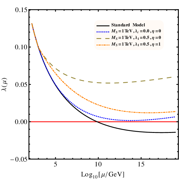
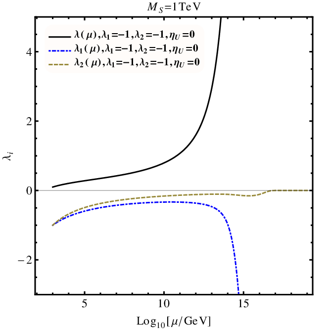
In the following we discuss the running of λ\lambda. We show in Fig. (1) how the scale of MSM_{S} can affect the running of λ\lambda. The solid line shows the original λ\lambda running behavior in the SM and it is evident that λ\lambda turns negative at a scale near 101010^{10}GeV 22 2 The precise scale depends on the mass of top quark mtm_{t} and strong coupling αs\alpha_{s}, a recent discussion on this can be found in Ref. [31, 32].. Now suppose that MS≃1​TeVM_{S}\simeq 1\textrm{TeV}, the effects of the color octet come into play when μ≥MS\mu\geq M_{S}, as shown in the dotted line. For ηU=0\eta_{U}=0, we have chosen λi=0\lambda_{i}=0 at MSM_{S} as illustration because this choice produces the minimal contributions to λ\lambda. It can still make λ\lambda positive, or the electroweak vacuum stable, up to the Planck scale. If MSM_{S} is very large, the color octet contributions come in too late and are not large enough to stabilize the vacuum, as shown in the dashed line. However, this could be amended very easily by non-vanishing λi\lambda_{i} as shown in the dot-dashed line which also shows a threshold effect.

It is interesting to note that even with λi=0\lambda_{i}=0 for ηU=0\eta_{U}=0, the color octet still modifies βλ\beta_{\lambda} through βgi\beta_{g_{i}} contributions as can be seen in the right panel of Fig. (1). Color octet effects will make the strong gauge couplings decrease slower than in the SM, and this serves as an additional positive contribution to βλ\beta_{\lambda}. Also, when the gauge couplings are larger, λ1,2\lambda_{1,2} would run away from zero faster because of the corresponding terms in Eq. (21) and Eq. (22). If the initial values of λi\lambda_{i} are not zero, the λi2\lambda_{i}^{2} terms in βλ\beta_{\lambda} give additional positive contributions and may be dominant in the running behavior of λ\lambda.

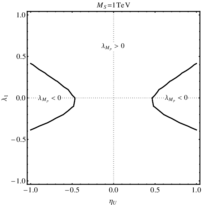
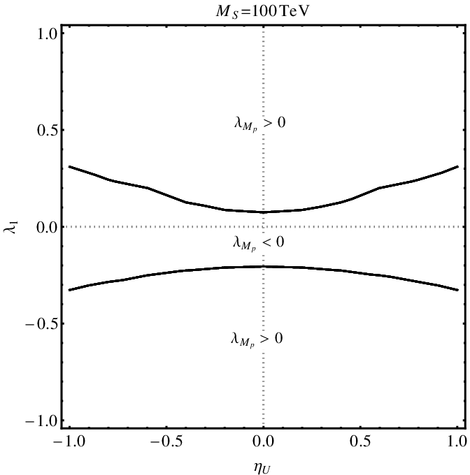
A non-vanishing ηU\eta_{U} has a negative contribution to the beta function of λ\lambda. In addition the positive contribution 43×32​ηU2​yt2\frac{4}{3}\times\frac{3}{2}\eta_{U}^{2}y_{t}^{2} in βyt\beta_{y_{t}} makes yty_{t} increase faster. This causes the top quark to decrease λ\lambda more effectively as the energy goes up. We show the running behavior of λ\lambda for ηU=1\eta_{U}=1 by the dot-dashed line in Fig. (1). As can be seen from the figure, if MSM_{S} is around the TeV scale and λi=0\lambda_{i}=0, the effects of enlarging η\eta would decrease the instability scale relative to that in the SM. The end result emerges from competition between non-vanishing ηU\eta_{U} and λi\lambda_{i}, and requiring λMP>0\lambda_{M_{P}}>0 (at the Planck mass) can constrain their ranges. We illustrate this with an example in Fig. 2 for some initial values of λ1\lambda_{1} and ηU\eta_{U}.

Refer to caption
Refer to caption
Figure 1: The running of the higgs quartic coupling in the standard model (solid line) and in the octet extension with various values of λi\lambda_{i} and ηU\eta_{U}. The figure on the left shows the effect of the scale MSM_{S} and the figure on the right shows the effect of sample values of λi\lambda_{i} and η≡ηU\eta\equiv\eta_{U}.
Refer to caption
Refer to caption
Figure 2: Sign of λMp\lambda_{M_{p}} (λ\lambda at the Planck scale) as contours on ηU\eta_{U} and λ1\lambda_{1} assuming vanishing λ2,3\lambda_{2,3} for two values of MSM_{S}. Similar constraints exist for ηU\eta_{U} and λ2\lambda_{2}.

V Renormalization group improved unitarity bounds

We can improve the unitarity constraints on the scalar self couplings obtained in Section III in some cases by considering their renormalization group evolution along the lines described in Ref. [33, 34] for the Higgs boson mass. In order to do this we need a complete set of one-loop beta functions which we provide in Appendix B. If we consider only one non-zero coupling at a time, that is we put all other λj=0​(j≠i)\lambda_{j}=0\ (j\neq i) in βλi\beta_{\lambda_{i}}, then except for λ4\lambda_{4}, the λi\lambda_{i} increase with energy and the corresponding unitarity bounds will be stronger. The solution of the complete set of coupled RGE is beyond the scope of this paper, but we illustrate the constraints that result in two restricted cases.

We first look at the sector of the potential responsible for the high energy h​h→S​Shh\to SS scattering at tree level, which in the limit of custodial symmetry is governed by the couplings λ1,2\lambda_{1,2}. The relevant RGE are

d​λ1d​ln⁡μ\displaystyle\frac{d\lambda_{1}}{d\ln\mu} =\displaystyle= 18​π2​(λ12+λ22)\displaystyle\frac{1}{8\pi^{2}}\left(\lambda_{1}^{2}+\lambda_{2}^{2}\right)
d​λ2d​ln⁡μ\displaystyle\frac{d\lambda_{2}}{d\ln\mu} =\displaystyle= 18​π2​λ2​(2​λ1+3​λ2).\displaystyle\frac{1}{8\pi^{2}}\lambda_{2}\left(2\lambda_{1}+3\lambda_{2}\right). (29)

These two coupled equations can be readily solved in terms of

a±=λ1+(32±132)​λ2,\displaystyle a_{\pm}=\lambda_{1}+\left(\frac{3}{2}\pm\frac{\sqrt{13}}{2}\right)\lambda_{2}, (30)

for which

a±​(μ)=a±​(μ0)1−18​π2​a±​(μ0)​ln⁡(μμ0).\displaystyle a_{\pm}(\mu)=\frac{a_{\pm}(\mu_{0})}{1-\frac{1}{8\pi^{2}}a_{\pm}(\mu_{0})\ln(\frac{\mu}{\mu_{0}})}. (31)

In Fig. 3 we show the region in the λ1−λ2\lambda_{1}-\lambda_{2} (at 1 TeV) plane that satisfies the unitarity constraint, Eq. 9 up to different energy scales. The red region corresponds to Eq. 9 for the couplings at 1 TeV indicating how there is no constraint along the direction λ2=−2​λ1\lambda_{2}=-2\lambda_{1}. In the green shaded region we require that the unitarity constraint be satisfied up to 100 TeV and in the blue shaded region up to 101010^{10} GeV. We see that as we require the theory to remain perturbative to higher scales, the allowed region for positive λ1,2\lambda_{1,2} shrinks as expected. On the other hand this does not happen for a region where one or both λ1,2\lambda_{1,2} are allowed to be negative. In Fig. 3 we also show the conditions a±=0a_{\pm}=0 with the dashed lines.

Refer to caption
Refer to caption
Figure 3: The left plot shows the region in the λ1−λ2\lambda_{1}-\lambda_{2} (at 1 TeV) plane that satisfies the unitarity constraint, Eq. 9 at 1 TeV in red, up to 100 TeV in green and up to 101010^{10} GeV in blue. The dashed lines show the conditions a±=0a_{\pm}=0. In the right plot, this region is further reduced by requiring unitarity up to 100 TeV in green and up to 101010^{10} GeV in blue for the λ−λ1,2\lambda-\lambda_{1,2} coupled system.

Next we recall that λ1,2\lambda_{1,2} contribute to the running of λ\lambda as in Eq. 20. We can solve numerically the coupled equations for λ\lambda and λ1,2\lambda_{1,2} by ignoring the other couplings and taking the custodial limit. If we then require that λ\lambda also satisfy its unitarity constraint [34] 5​λ/(16​π)≤1/25\lambda/(16\pi)\leq 1/2, we further restrict the allowed parameter space. The area in the λ1−λ2\lambda_{1}-\lambda_{2} plane that is allowed in this case is shown in the right side of Fig. 3.

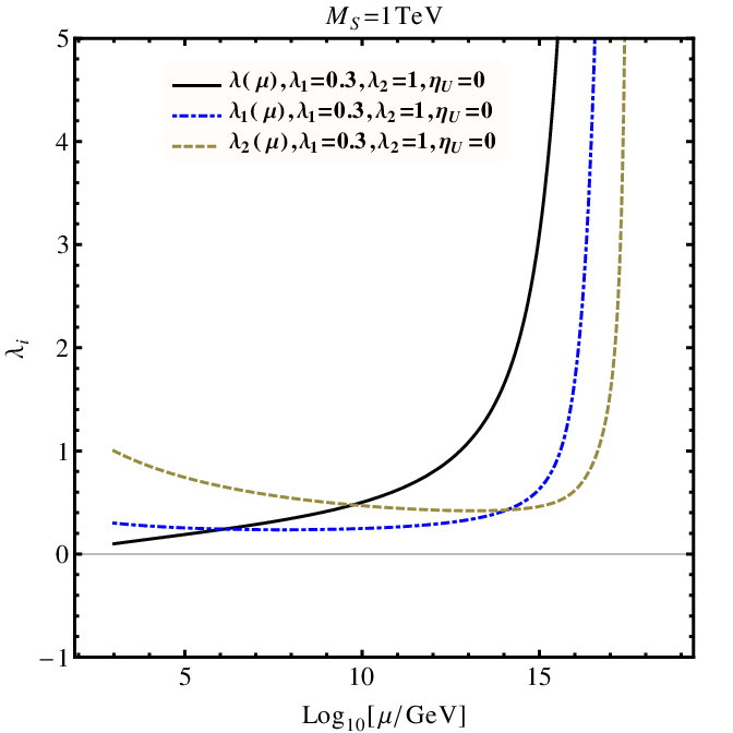
In the above discussion we have neglected the gauge coupling contributions to the RGE. The effects of the gauge couplings, dominated by the strong coupling, tend to slow down the raising of λ1,2\lambda_{1,2} which in turn slows down the growing rate for λ\lambda. Therefore one expects that inclusion of the gauge couplings will delay the reach of the unitarity bounds. In Fig. 4 we use two sets of typical initial values from the blue region in Fig. 3 as illustration, to show the running behavior of λ\lambda and λ1,2\lambda_{1,2}. We see that indeed λ\lambda and λ1,2\lambda_{1,2} are below the unitarity bounds all the way up to a scale higher than 101010^{10} GeV.

Refer to caption
Refer to caption
Figure 4: Illustration of running behaviors of λi\lambda_{i} and λ\lambda.

Finally we study the sector with λ8,9,11\lambda_{8,9,11} responsible for high energy scattering S​S→S​SSS\to SS at tree level in the custodial symmetry limit. The corresponding RGE are given by

d​λ8d​ln⁡μ\displaystyle\frac{d\lambda_{8}}{d\ln\mu} =\displaystyle= 1144​π2​(180​λ82+234​λ8​(λ9+λ11)+54​λ92+67​λ112)\displaystyle\frac{1}{144\pi^{2}}(180\lambda_{8}^{2}+234\lambda_{8}(\lambda_{9}+\lambda_{11})+54\lambda_{9}^{2}+67\lambda_{11}^{2})
d​λ9d​ln⁡μ\displaystyle\frac{d\lambda_{9}}{d\ln\mu} =\displaystyle= 1144​π2​(144​λ92+54​λ8​λ9+78​λ9​λ11+λ112)\displaystyle\frac{1}{144\pi^{2}}(144\lambda_{9}^{2}+54\lambda_{8}\lambda_{9}+78\lambda_{9}\lambda_{11}+\lambda_{11}^{2})
d​λ11d​ln⁡μ\displaystyle\frac{d\lambda_{11}}{d\ln\mu} =\displaystyle= 132​π2​(13​λ112+12​λ8​λ11+12​λ9​λ11)\displaystyle\frac{1}{32\pi^{2}}(13\lambda_{11}^{2}+12\lambda_{8}\lambda_{11}+12\lambda_{9}\lambda_{11}) (32)

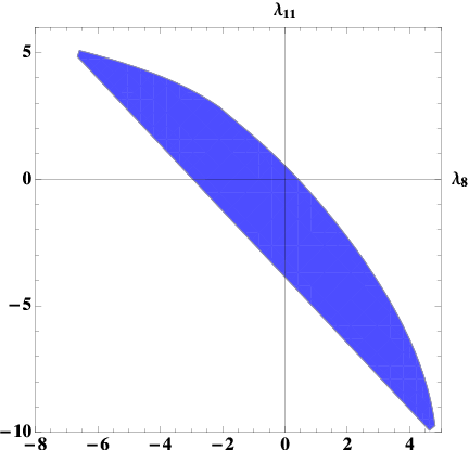
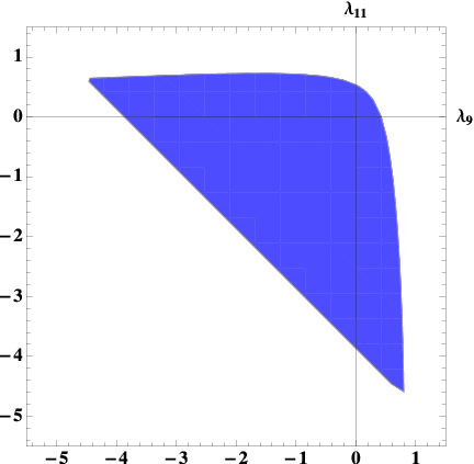
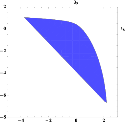
This set of coupled equations can be solved numerically and we obtain results that are qualitatively similar to the ones for λ1,2\lambda_{1,2}. As we require the unitarity constraints to be satisfied to higher energies, the allowed parameter space for positive values of λ8,9,11\lambda_{8,9,11} shrinks and they are constrained to be small. In Fig. 5 we show our numerical solution for the allowed regions in λ8,9,11\lambda_{8,9,11} (at 1 TeV) that satisfy the unitarity constraints Eqs. 14, 17, and 35 up to 101010^{10} GeV by taking two of them to be non-zero at a time as the blue region.
Refer to caption
Refer to caption
Refer to caption
Figure 5: Allowed regions in λ8,9,11\lambda_{8,9,11} (at 1 TeV) that satisfy the unitarity constraints Eqs. 14, 17, 35 up to 101010^{10} GeV by taking two of them to be non-zero at a time shown in the blue region.

VI Numerical values for color-octet couplings used in the literature

In this section we briefly review some of the phenomenological applications of this color-octet model that have appeared in the literature with emphasis on the numerical values used for the different couplings.

In their original paper Manohar and Wise [24] point out that the values λ1=4\lambda_{1}=4 and λ2=1\lambda_{2}=1 for mS=750m_{S}=750 GeV can increase the Higgs production rate by a factor of 2 while decreasing H→γ​γH\to\gamma\gamma by 10% and being consistent with constraints from the SS parameter.

In [35], it is found that the contributions of the model to RbR_{b} imply that for masses in the mS∼1​(4)m_{S}\sim 1\ (4) TeV region, |ηU|   <  ∼  1.8​(5)|\eta_{U}|\mathrel{\vbox{\kern 0.0pt\hbox{$<$} \kern 0.0pt\hbox{$\sim$} }}1.8\ (5) to stay within 2σ\sigma of the measured value. They also compute the singlet color octet production rate at LHC assuming λ4,5∼1\lambda_{4,5}\sim 1 and |ηU|=1|\eta_{U}|=1.

In [36], the minimum values of |λ2±2​λ3||\lambda_{2}\pm 2\lambda_{3}| and of |λ3||\lambda_{3}| that allow for two body decays of the color octet states involving W±W^{\pm} are calculated. For a min⁡{mS±,mSi,r}{\rm min}\{m_{S^{\pm}},m_{S_{i,r}}\} in the range 200−600200-600 GeV, |λ2±2​λ3|min∼(2−6)|\lambda_{2}\pm 2\lambda_{3}|_{\rm min}\sim(2-6) for example. In addition they also consider the running of the couplings λi\lambda_{i} and find constraints by requiring that they remain perturbative up to some scale which they use to study color octet phenomenology at LHC. We disagree with their beta-functions as given in their appendix so the constraints that we obtain are different.

In [26], the mass splittings between M+,MR,MIM_{+},M_{R},M_{I} are studied imposing constraints from electroweak precision data and allowed regions are presented for λ1,2,3\lambda_{1,2,3} as large as 10. Requiring that there be no Landau pole in the running of λ\lambda up to 10 TeV results in λ1   <  ∼  1.3\lambda_{1}\mathrel{\vbox{\kern 0.0pt\hbox{$<$} \kern 0.0pt\hbox{$\sim$} }}1.3 and λ12+λ22   <  ∼  2.2\sqrt{\lambda_{1}^{2}+\lambda_{2}^{2}}\mathrel{\vbox{\kern 0.0pt\hbox{$<$} \kern 0.0pt\hbox{$\sim$} }}2.2. They also point out the electric dipole moment of the neutron for light masses mS=100m_{S}=100 GeV implies that Im⁡(ηU⋆​ηD⋆)<0.1{\rm Im}(\eta_{U}^{\star}\eta_{D}^{\star})<0.1. Finally they argue that λ4,5<10\lambda_{4,5}<10 to remain in the perturbative regime.

Several studies use this model to modify jet production. For example, in [27, 37], this model is studied in connection with the CDF diet anomaly. The production cross section of SR0S_{R}^{0} is calculated as function of λ4+λ5\lambda_{4}+\lambda_{5}, ranging from 0 to 30. For the benchmark point of MR=245M_{R}=245 GeV, MI=190M_{I}=190 GeV, M±=150M_{\pm}=150 GeV, λ4+λ5=18\lambda_{4}+\lambda_{5}=18 is needed to explain the CDF anomaly. In Ref. [38] several multi jet process are studied with λ4,5∼1\lambda_{4,5}\sim 1 and λ1,2,3∼1/2\lambda_{1,2,3}\sim 1/2.

Several papers have studied this model in relation to possible enhancements/suppressions of the Higgs coupling to gluons or photons. In Ref. [39] it is argued that this model can reduce the Higgs production cross section at LHC to make it compatible with a fourth generation. Saturating the SS parameter with λ2\lambda_{2} results in the constraint for mS∼1m_{S}\sim 1 TeV, −48   <  ∼  λ2   <  ∼  6-48\mathrel{\vbox{\kern 0.0pt\hbox{$<$} \kern 0.0pt\hbox{$\sim$} }}\lambda_{2}\mathrel{\vbox{\kern 0.0pt\hbox{$<$} \kern 0.0pt\hbox{$\sim$} }}6. Using this constraint on λ2\lambda_{2} it is found that λ1∼−8\lambda_{1}\sim-8 would be needed to halve the SM4 h​g​ghgg coupling for masses mS∼2​vm_{S}\sim 2v. A similar argument for reducing the Higgs production cross section in the SM was presented in Ref. [40] and one for hiding heavier Higgs bosons in Ref. [41]. Ref. [42] uses similar models to enhance the H→γ​γH\to\gamma\gamma rate and Ref. [43] to enhance di-Higgs production.

In Ref. [44] it is pointed out that this model can result in large CP violation in top pair production at the LHC. The parameter range considered was λ4,5   <  ∼  8\lambda_{4,5}\mathrel{\vbox{\kern 0.0pt\hbox{$<$} \kern 0.0pt\hbox{$\sim$} }}8 and large phases in λ4\lambda_{4} and ηU\eta_{U}. It was also found that for color octet resonances with masses in the 500−1000500-1000 GeV range one needed ηU∼3\eta_{U}\sim 3 to have them stand out over QCD background.

In [45] the h​g​ghgg and h​γ​γh\gamma\gamma couplings as fit from LHC data are compared with sample BSM scenarios. Although no attempt is made to constrain the couplings of the color octet model, it is shown that it is consistent with data using ms=750m_{s}=750 GeV for values λ1=4,λ2=1\lambda_{1}=4,\lambda_{2}=1.

In Ref. [46] the possibility of inverting the sign of the h​g​ghgg coupling with additional color octets is studied and the allowed parameter space has λO   >  ∼  4\lambda_{O}\mathrel{\vbox{\kern 0.0pt\hbox{$>$} \kern 0.0pt\hbox{$\sim$} }}4 where λO\lambda_{O} corresponds to λ8\lambda_{8} in Eq. 3.

Finally, in the very recent Ref. [47] the model is considered in connection to LHC Higgs data. They examine the constraints imposed on the model by unitarity numerically and find that for mh=125.5m_{h}=125.5 GeV |λ1,2|   <  ∼  35|\lambda_{1,2}|\mathrel{\vbox{\kern 0.0pt\hbox{$<$} \kern 0.0pt\hbox{$\sim$} }}35 and |λ3|   <  ∼  18|\lambda_{3}|\mathrel{\vbox{\kern 0.0pt\hbox{$<$} \kern 0.0pt\hbox{$\sim$} }}18, worse than our limits by factors between 2 and 4.

Color octet scalars also appear in specific models considered recently [48].

VII Summary and Conclusions

In this paper we have examined the theoretical constraints on the color-octet extension of the standard model scalar sector. We first required perturbative unitarity for two-to-two scalar scattering amplitudes to obtain general bounds for the parameters in the scalar potential. We then considered the renormalization group equations for the couplings and used this to provide constraints from the requirement of a stable vacuum up to high energy. An amusing fact is that for octet masses near a TeV, even with vanishing couplings to quarks and the higgs boson, the electroweak vacuum can be stabilized up to the Planck scale. Finally we considered improvement of our unitarity constraints by requiring they be satisfied up to high energy scales. This consideration further constrains the values allowed. Finally we reviewed some of the phenomenological studies that have used this model in the literature and found that many of them stray outside the theoretical constraints found here. Our results should prove useful for future phenomenology of this model.

Acknowledgements.
The work of XGH and YT was supported in part by NSC of ROC, and XGH was also supported in part by NNSF(grant No:11175115) and Shanghai science and technology commission (grant No: 11DZ2260700) of PRC. The work of GV and HP was supported in part by DOE under contract number DE-FG02-01ER41155.

Appendix A Partial wave amplitudes in the general case without custodial symmetry

We begin by displaying results for h​h→S​Shh\to SS partial wave amplitudes in the high energy limit in Table 1.

Table 1: J=0J=0 partial wave amplitudes for the scattering of the different neutral combinations of h​h→S​Shh\to SS in a color singlet state.
channel 8​2​π​aJ=008\sqrt{2}\pi\ a^{0}_{J=0}
w+​w−→S+​S−w^{+}w^{-}\to S^{+}S^{-} λ1+λ2\lambda_{1}+\lambda_{2}
w+​w−→Si​Siw^{+}w^{-}\to S_{i}S_{i} = w+​w−→Sr​Srw^{+}w^{-}\to S_{r}S_{r} = z​z→S+​S−zz\to S^{+}S^{-} = h​h→S+​S−hh\to S^{+}S^{-} λ1\lambda_{1}
z​z→Si​Sizz\to S_{i}S_{i} = h​h→Sr​Srhh\to S_{r}S_{r} λ1+λ2+2​λ3\lambda_{1}+\lambda_{2}+2\lambda_{3}
z​z→Sr​Srzz\to S_{r}S_{r} = h​h→Si​Sihh\to S_{i}S_{i} λ1+λ2−2​λ3\lambda_{1}+\lambda_{2}-2\lambda_{3}

Inspection of the partial wave amplitudes presented in Table 1 reveals that Eq. 8 is obtained by adding all the channels (with a suitable normalization). Other possible combinations include

a​((z​z+h​h)/2→(Si​Si+Sr​Sr)/2)J=00\displaystyle a((zz+hh)/2\to(S_{i}S_{i}+S_{r}S_{r})/2)_{J=0}^{0} =\displaystyle= (λ1+λ2)8​2​π\displaystyle\frac{(\lambda_{1}+\lambda_{2})}{8\sqrt{2}\pi}
a​((z​z−h​h)/2→Si​Si)J=00\displaystyle a((zz-hh)/2\to S_{i}S_{i})_{J=0}^{0} =\displaystyle= λ34​2​π.\displaystyle\frac{\lambda_{3}}{4\sqrt{2}\pi}. (33)

From the last of these conditions we obtain Eq. 10, and from the second row in Table 1 we obtain λ1   <  ∼  18\lambda_{1}\mathrel{\vbox{\kern 0.0pt\hbox{$<$} \kern 0.0pt\hbox{$\sim$} }}18.

Next we consider the scattering of S​S→S​SSS\to SS to constrain λ4−11\lambda_{4-11} and display the results for J=0J=0 partial wave amplitudes in Table 2.

Table 2: J=0J=0 partial wave amplitudes for the scattering of the different neutral combinations of S​S→S​SSS\to SS in a color singlet state.
channel 96​π​aJ=0096\pi\ a^{0}_{J=0}
S+​S−→S+​S−S^{+}S^{-}\to S^{+}S^{-} 6​λ10+7​λ11+16​λ6+16​λ7+27​λ8+27​λ96\lambda_{10}+7\lambda_{11}+16\lambda_{6}+16\lambda_{7}+27\lambda_{8}+27\lambda_{9}
Si​Si→Si​SiS_{i}S_{i}\to S_{i}S_{i} = Sr​Sr→Sr​SrS_{r}S_{r}\to S_{r}S_{r} 30​λ10+15​λ11+15​λ6+15​λ7+30​λ8+30​λ930\lambda_{10}+15\lambda_{11}+15\lambda_{6}+15\lambda_{7}+30\lambda_{8}+30\lambda_{9}
Si​Si→S+​S−S_{i}S_{i}\to S^{+}S^{-} = Sr​Sr→S+​S−S_{r}S_{r}\to S^{+}S^{-} 3​λ10+8​λ11+8​λ6+8​λ7+24​λ8+3​λ93\lambda_{10}+8\lambda_{11}+8\lambda_{6}+8\lambda_{7}+24\lambda_{8}+3\lambda_{9}
Si​Si→Sr​SrS_{i}S_{i}\to S_{r}S_{r} 3​λ10−λ11+17​λ6+17​λ7+24​λ8+3​λ93\lambda_{10}-\lambda_{11}+17\lambda_{6}+17\lambda_{7}+24\lambda_{8}+3\lambda_{9}

In the custodial symmetry limit the corresponding results are shown in Table 3.

Table 3: J=0J=0 partial wave amplitudes for the scattering of the different neutral combinations of S​S→S​SSS\to SS in a color singlet state in the custodial symmetry limit.
channel 96​π​aJ=0096\pi\ a^{0}_{J=0}
S+​S−→S+​S−S^{+}S^{-}\to S^{+}S^{-} 23​λ11+27​λ8+33​λ923\lambda_{11}+27\lambda_{8}+33\lambda_{9}
Si​Si→Si​SiS_{i}S_{i}\to S_{i}S_{i} = Sr​Sr→Sr​SrS_{r}S_{r}\to S_{r}S_{r} 30​λ11+30​λ8+60​λ930\lambda_{11}+30\lambda_{8}+60\lambda_{9}
Si​Si→S+​S−S_{i}S_{i}\to S^{+}S^{-} = Sr​Sr→S+​S−S_{r}S_{r}\to S^{+}S^{-} = Si​Si→Sr​SrS_{i}S_{i}\to S_{r}S_{r} 16​λ11+24​λ8+6​λ916\lambda_{11}+24\lambda_{8}+6\lambda_{9}

Weaker bounds arise from considering color octet (or 27) channels but they can be useful to place separate constraints on particular couplings. For illustration we include one such channel in the antisymmetric color octet

a0(+−)0\displaystyle a^{0}_{(+-)0} =\displaystyle= a​(12​(S+​S−−S−​S+)→12​(S+​S−−S−​S+))J=08​A\displaystyle a(\frac{1}{\sqrt{2}}(S^{+}S^{-}-S^{-}S^{+})\to\frac{1}{\sqrt{2}}(S^{+}S^{-}-S^{-}S^{+}))_{J=0}^{8A} (34)
=\displaystyle= 132​π​(2​λ8−2​λ9+3​λ11)+332​π​v2(s−ms2)​λ42​sin2⁡(ϕ4)\displaystyle\frac{1}{32\pi}(2\lambda_{8}-2\lambda_{9}+3\lambda_{11})+\frac{3}{32\pi}\frac{v^{2}}{(s-m_{s}^{2})}\lambda_{4}^{2}\sin^{2}(\phi_{4})
−\displaystyle- 132​π​v2(s−ms2)​λ12​log⁡(s−4​ms2+mH2mH2)\displaystyle\frac{1}{32\pi}\frac{v^{2}}{(s-m_{s}^{2})}\lambda_{1}^{2}\log\left(\frac{s-4m_{s}^{2}+m_{H}^{2}}{m_{H}^{2}}\right)
−\displaystyle- 1192​π​v2(s−4​ms2)​λ42​(7−2​cos⁡(2​ϕ4))​log⁡(s−3​ms2ms2)\displaystyle\frac{1}{192\pi}\frac{v^{2}}{(s-4m_{s}^{2})}\lambda_{4}^{2}(7-2\cos(2\phi_{4}))\log\left(\frac{s-3m_{s}^{2}}{m_{s}^{2}}\right)

from which one finds

|2​λ8−2​λ9+3​λ11|   <  ∼  16​π.\displaystyle\left|2\lambda_{8}-2\lambda_{9}+3\lambda_{11}\right|\mathrel{\vbox{\kern 0.0pt\hbox{$<$} \kern 0.0pt\hbox{$\sim$} }}16\pi. (35)

Appendix B β\beta functions without custodial symmetry

Using the techniques in ref. [49, 50], one can easily obtain the relevent β\beta functions. Here we give the color octet contributions to the β\beta functions for λ\lambdas in the general case without custodial symmetry,

(16​π2)​βλ1\displaystyle(16\pi^{2})\beta_{\lambda_{1}} =\displaystyle= 2​λ12+λ22+4​λ32+4​λ​(3​λ1+λ2)\displaystyle 2\lambda_{1}^{2}+\lambda_{2}^{2}+4\lambda_{3}^{2}+4\lambda(3\lambda_{1}+\lambda_{2})
+13​(7​λ4​λ4∗−2​λ4∗​λ5−2​λ5∗​λ4+7​λ5​λ5∗)\displaystyle{}+\frac{1}{3}(7\lambda_{4}\lambda_{4}^{*}-2\lambda_{4}^{*}\lambda_{5}-2\lambda_{5}^{*}\lambda_{4}+7\lambda_{5}\lambda_{5}^{*})
+λ1​(8​λ6+8​λ7+17​λ8+10​λ9+3​λ10+5​λ11)\displaystyle{}+\lambda_{1}(8\lambda_{6}+8\lambda_{7}+17\lambda_{8}+10\lambda_{9}+3\lambda_{10}+5\lambda_{11})
+13​λ2​(8​λ6+8​λ7+24​λ8+3​λ9+3​λ10+8​λ11),\displaystyle{}+\frac{1}{3}\lambda_{2}(8\lambda_{6}+8\lambda_{7}+24\lambda_{8}+3\lambda_{9}+3\lambda_{10}+8\lambda_{11}),
(16​π2)​βλ2\displaystyle(16\pi^{2})\beta_{\lambda_{2}} =\displaystyle= 2​λ22+4​λ1​λ2+16​λ32+4​λ​λ2\displaystyle 2\lambda_{2}^{2}+4\lambda_{1}\lambda_{2}+16\lambda_{3}^{2}+4\lambda\lambda_{2}
+16​(8​λ4​λ4∗+17​λ4∗​λ5+17​λ5∗​λ4+8​λ5​λ5∗)\displaystyle{}+\frac{1}{6}(8\lambda_{4}\lambda_{4}^{*}+17\lambda_{4}^{*}\lambda_{5}+17\lambda_{5}^{*}\lambda_{4}+8\lambda_{5}\lambda_{5}^{*})
+16​λ2​(16​λ6+16​λ7+6​λ8+48​λ9+6​λ10−2​λ11),\displaystyle{}+\frac{1}{6}\lambda_{2}(16\lambda_{6}+16\lambda_{7}+6\lambda_{8}+48\lambda_{9}+6\lambda_{10}-2\lambda_{11}),
(16​π2)​βλ3\displaystyle(16\pi^{2})\beta_{\lambda_{3}} =\displaystyle= 2​λ3​(2​λ+2​λ1+3​λ2)+112​(17​λ42+16​λ4​λ5+17​λ52)\displaystyle 2\lambda_{3}(2\lambda+2\lambda_{1}+3\lambda_{2})+\frac{1}{12}(17\lambda_{4}^{2}+16\lambda_{4}\lambda_{5}+17\lambda_{5}^{2})
+13​λ3​(−λ6−λ7+3​λ8+3​λ9+24​λ10+8​λ11),\displaystyle{}+\frac{1}{3}\lambda_{3}(-\lambda_{6}-\lambda_{7}+3\lambda_{8}+3\lambda_{9}+24\lambda_{10}+8\lambda_{11}),
(16​π2)​βλ4\displaystyle(16\pi^{2})\beta_{\lambda_{4}} =\displaystyle= 8​λ4∗​λ3+2​λ3​λ5∗+λ5​(2​λ2−λ7+2​λ9+4​λ10+λ11)\displaystyle 8\lambda_{4}^{*}\lambda_{3}+2\lambda_{3}\lambda_{5}^{*}+\lambda_{5}(2\lambda_{2}-\lambda_{7}+2\lambda_{9}+4\lambda_{10}+\lambda_{11})
+λ4​(3​λ1+2​λ2+6​λ6+2​λ7+3​λ8+2​λ9+λ10+λ11),\displaystyle+\lambda_{4}(3\lambda_{1}+2\lambda_{2}+6\lambda_{6}+2\lambda_{7}+3\lambda_{8}+2\lambda_{9}+\lambda_{10}+\lambda_{11}),
(16​π2)​βλ5\displaystyle(16\pi^{2})\beta_{\lambda_{5}} =\displaystyle= 2​λ3​λ4∗+8​λ3​λ5∗+λ4​(2​λ2−λ6+2​λ9+4​λ10+λ11)\displaystyle 2\lambda_{3}\lambda_{4}^{*}+8\lambda_{3}\lambda_{5}^{*}+\lambda_{4}(2\lambda_{2}-\lambda_{6}+2\lambda_{9}+4\lambda_{10}+\lambda_{11})
+λ5​(3​λ1+2​λ2+6​λ6+2​λ7+3​λ8+2​λ9+λ10+λ11),\displaystyle+\lambda_{5}(3\lambda_{1}+2\lambda_{2}+6\lambda_{6}+2\lambda_{7}+3\lambda_{8}+2\lambda_{9}+\lambda_{10}+\lambda_{11}),
(16​π2)​βλ6\displaystyle(16\pi^{2})\beta_{\lambda_{6}} =\displaystyle= 3​λ4​λ4∗+7​λ62+λ6​(6​λ7+6​λ8+4​λ9−λ10−2​λ11)\displaystyle 3\lambda_{4}\lambda_{4}^{*}+7\lambda_{6}^{2}+\lambda_{6}(6\lambda_{7}+6\lambda_{8}+4\lambda_{9}-\lambda_{10}-2\lambda_{11})
+λ7​(4​λ9−λ10)−2​λ9​λ11+2​λ10​λ11+λ112,\displaystyle+\lambda_{7}(4\lambda_{9}-\lambda_{10})-2\lambda_{9}\lambda_{11}+2\lambda_{10}\lambda_{11}+\lambda_{11}^{2},
(16​π2)​βλ7\displaystyle(16\pi^{2})\beta_{\lambda_{7}} =\displaystyle= 3​λ5​λ5∗+7​λ72+λ7​(6​λ6+6​λ8+4​λ9−λ10−2​λ11)\displaystyle 3\lambda_{5}\lambda_{5}^{*}+7\lambda_{7}^{2}+\lambda_{7}(6\lambda_{6}+6\lambda_{8}+4\lambda_{9}-\lambda_{10}-2\lambda_{11})
+λ6​(4​λ9−λ10)−2​λ9​λ11+2​λ10​λ11+λ112,\displaystyle+\lambda_{6}(4\lambda_{9}-\lambda_{10})-2\lambda_{9}\lambda_{11}+2\lambda_{10}\lambda_{11}+\lambda_{11}^{2},
(16​π2)​βλ8\displaystyle(16\pi^{2})\beta_{\lambda_{8}} =\displaystyle= 20​λ82+118​λ8​(288​λ6+288​λ7+360​λ9+108​λ10+180​λ11)\displaystyle 20\lambda_{8}^{2}+\frac{1}{18}\lambda_{8}(288\lambda_{6}+288\lambda_{7}+360\lambda_{9}+108\lambda_{10}+180\lambda_{11})
+118[36λ12+36λ1λ2−24λ4λ4∗−6λ4∗λ5−6λ5∗λ4−24λ5λ5∗\displaystyle+\frac{1}{18}[36\lambda_{1}^{2}+36\lambda_{1}\lambda_{2}-24\lambda_{4}\lambda_{4}^{*}-6\lambda_{4}^{*}\lambda_{5}-6\lambda_{5}^{*}\lambda_{4}-24\lambda_{5}\lambda_{5}^{*}
+62​λ62+64​λ6​λ7+62​λ72+96​λ9​(λ6+λ7)+18​λ10​(λ6+λ7)+58​λ11​(λ6+λ7)\displaystyle+62\lambda_{6}^{2}+64\lambda_{6}\lambda_{7}+62\lambda_{7}^{2}+96\lambda_{9}(\lambda_{6}+\lambda_{7})+18\lambda_{10}(\lambda_{6}+\lambda_{7})+58\lambda_{11}(\lambda_{6}+\lambda_{7})
+54λ92+36λ9λ10+132λ9λ11+18λ102+18λ10λ11+29λ112],\displaystyle+54\lambda_{9}^{2}+36\lambda_{9}\lambda_{10}+132\lambda_{9}\lambda_{11}+18\lambda_{10}^{2}+18\lambda_{10}\lambda_{11}+29\lambda_{11}^{2}],
(16​π2)​βλ9\displaystyle(16\pi^{2})\beta_{\lambda_{9}} =\displaystyle= λ22−13​(λ4​λ4∗−2​λ4∗​λ5−2​λ5∗​λ4+λ5​λ5∗)+10​λ92\displaystyle\lambda_{2}^{2}-\frac{1}{3}(\lambda_{4}\lambda_{4}^{*}-2\lambda_{4}^{*}\lambda_{5}-2\lambda_{5}^{*}\lambda_{4}+\lambda_{5}\lambda_{5}^{*})+10\lambda_{9}^{2}
+λ10​(λ6+λ7+λ11)+λ9​[43​(4​λ6+4​λ7+λ11)+2​λ10+6​λ9]\displaystyle+\lambda_{10}(\lambda_{6}+\lambda_{7}+\lambda_{11})+\lambda_{9}[\frac{4}{3}(4\lambda_{6}+4\lambda_{7}+\lambda_{11})+2\lambda_{10}+6\lambda_{9}]
+4​λ102+19​(λ62+λ72−4​λ11​(λ6+λ7)−2​λ112)+269​λ6​λ7,\displaystyle+4\lambda_{10}^{2}+\frac{1}{9}(\lambda_{6}^{2}+\lambda_{7}^{2}-4\lambda_{11}(\lambda_{6}+\lambda_{7})-2\lambda_{11}^{2})+\frac{26}{9}\lambda_{6}\lambda_{7},
(16​π2)​βλ10\displaystyle(16\pi^{2})\beta_{\lambda_{10}} =\displaystyle= 4​λ32−13​(λ4​λ4∗−2​λ4∗​λ5−2​λ5∗​λ4+λ5​λ5∗)\displaystyle 4\lambda_{3}^{2}-\frac{1}{3}(\lambda_{4}\lambda_{4}^{*}-2\lambda_{4}^{*}\lambda_{5}-2\lambda_{5}^{*}\lambda_{4}+\lambda_{5}\lambda_{5}^{*})
+λ10​[13​(λ6+λ7+19​λ11)+8​λ9+6​λ8]+2​λ9​λ11+8​λ102\displaystyle+\lambda_{10}[\frac{1}{3}(\lambda_{6}+\lambda_{7}+19\lambda_{11})+8\lambda_{9}+6\lambda_{8}]+2\lambda_{9}\lambda_{11}+8\lambda_{10}^{2}
+19​(λ62+λ72−4​λ11​(λ6+λ7)+7​λ112)−109​λ6​λ7,\displaystyle+\frac{1}{9}(\lambda_{6}^{2}+\lambda_{7}^{2}-4\lambda_{11}(\lambda_{6}+\lambda_{7})+7\lambda_{11}^{2})-\frac{10}{9}\lambda_{6}\lambda_{7},

and finally

(16​π2)​βλ11\displaystyle(16\pi^{2})\beta_{\lambda_{11}} =\displaystyle= 12​λ112+3​λ4​λ4∗+3​λ5​λ5∗−2​(λ62+λ72)+6​λ10​(λ6+λ7)+7​λ11​(λ6+λ7+λ8).\displaystyle\frac{1}{2}\lambda_{11}^{2}+3\lambda_{4}\lambda_{4}^{*}+3\lambda_{5}\lambda_{5}^{*}-2(\lambda_{6}^{2}+\lambda_{7}^{2})+6\lambda_{10}(\lambda_{6}+\lambda_{7})+7\lambda_{11}(\lambda_{6}+\lambda_{7}+\lambda_{8}).

References

  • [1] G. Aad et al. [ATLAS Collaboration], Phys. Lett. B 716, 1 (2012) [arXiv:1207.7214 [hep-ex]].
  • [2] S. Chatrchyan et al. [CMS Collaboration], Phys. Lett. B 716, 30 (2012) [arXiv:1207.7235 [hep-ex]].
  • [3] M. Holthausen, K. S. Lim and M. Lindner, JHEP 1202 (2012) 037 [arXiv:1112.2415 [hep-ph]].
  • [4] Z. -z. Xing, H. Zhang and S. Zhou, Phys. Rev. D 86, 013013 (2012) [arXiv:1112.3112 [hep-ph]].
  • [5] G. Degrassi, S. Di Vita, J. Elias-Miro, J. R. Espinosa, G. F. Giudice, G. Isidori and A. Strumia, JHEP 1208, 098 (2012) [arXiv:1205.6497 [hep-ph]].
  • [6] F. Bezrukov, M. Y. .Kalmykov, B. A. Kniehl and M. Shaposhnikov, JHEP 1210 (2012) 140 [arXiv:1205.2893 [hep-ph]].
  • [7] Y. Tang, arXiv:1301.5812 [hep-ph], and references therein.
  • [8] C. -S. Chen and Y. Tang, JHEP 1204, 019 (2012) [arXiv:1202.5717 [hep-ph]].
  • [9] J. Elias-Miro, J. R. Espinosa, G. F. Giudice, H. M. Lee and A. Strumia, JHEP 1206, 031 (2012) [arXiv:1203.0237 [hep-ph]].
  • [10] O. Lebedev, Eur. Phys. J. C 72, 2058 (2012) [arXiv:1203.0156 [hep-ph]].
  • [11] W. Rodejohann and H. Zhang, JHEP 1206, 022 (2012) [arXiv:1203.3825 [hep-ph]].
  • [12] C. Cheung, M. Papucci and K. M. Zurek, JHEP 1207, 105 (2012) [arXiv:1203.5106 [hep-ph]].
  • [13] K. Kannike, Eur. Phys. J. C 72, 2093 (2012) [arXiv:1205.3781 [hep-ph]].
  • [14] W. Chao, M. Gonderinger and M. J. Ramsey-Musolf, Phys. Rev. D 86, 113017 (2012) [arXiv:1210.0491 [hep-ph]].
  • [15] S. Iso and Y. Orikasa, PTEP 2013 (2013) 023B08 [arXiv:1210.2848 [hep-ph]].
  • [16] K. Allison, arXiv:1210.6852 [hep-ph];
  • [17] G. Belanger, K. Kannike, A. Pukhov and M. Raidal, arXiv:1211.1014 [hep-ph].
  • [18] H. H. Patel and M. J. Ramsey-Musolf, arXiv:1212.5652 [hep-ph].
  • [19] W. Chao, J. -H. Zhang and Y. Zhang, arXiv:1212.6272 [hep-ph].
  • [20] P. S. B. Dev, D. K. Ghosh, N. Okada and I. Saha, arXiv:1301.3453 [hep-ph].
  • [21] A. Goudelis, B. Herrmann and O. Stål, arXiv:1303.3010 [hep-ph].
  • [22] R. S. Chivukula and H. Georgi, Phys. Lett. B 188 (1987) 99.
  • [23] G. D’Ambrosio, G. F. Giudice, G. Isidori and A. Strumia, Nucl. Phys. B 645 (2002) 155 [hep-ph/0207036].
  • [24] A. V. Manohar and M. B. Wise, Phys. Rev. D 74, 035009 (2006) [hep-ph/0606172].
  • [25] Xiao-Gang He, Yong Tang and German Valencia, Higgs phenomenology in the presence of a scalar color, in preparation.
  • [26] C. P. Burgess, M. Trott and S. Zuberi, JHEP 0909, 082 (2009) [arXiv:0907.2696 [hep-ph]].
  • [27] L. M. Carpenter and S. Mantry, Phys. Lett. B 703, 479 (2011) [arXiv:1104.5528 [hep-ph]].
  • [28] B. W. Lee, C. Quigg and H. B. Thacker, Phys. Rev. D 16, 1519 (1977).
  • [29] S. Kanemura, T. Kubota and E. Takasugi, Phys. Lett. B 313, 155 (1993) [hep-ph/9303263].
  • [30] J. Bulava, P. Gerhold, K. Jansen, J. Kallarackal, B. Knippschild, C. -J. D. Lin, K. -I. Nagai and A. Nagy et al., arXiv:1210.1798 [hep-lat].
  • [31] S. Alekhin, A. Djouadi and S. Moch, Phys. Lett. B 716 (2012) 214 [arXiv:1207.0980 [hep-ph]].
  • [32] I. Masina, arXiv:1209.0393 [hep-ph].
  • [33] M. S. Chanowitz, M. A. Furman and I. Hinchliffe, Phys. Lett. B 78 (1978) 285.
  • [34] W. J. Marciano, G. Valencia and S. Willenbrock, Phys. Rev. D 40, 1725 (1989).
  • [35] M. I. Gresham and M. B. Wise, Phys. Rev. D 76, 075003 (2007) [arXiv:0706.0909 [hep-ph]].
  • [36] M. Gerbush, T. J. Khoo, D. J. Phalen, A. Pierce and D. Tucker-Smith, Phys. Rev. D 77, 095003 (2008) [arXiv:0710.3133 [hep-ph]].
  • [37] T. Enkhbat, X. -G. He, Y. Mimura and H. Yokoya, JHEP 1202, 058 (2012) [arXiv:1105.2699 [hep-ph]].
  • [38] J. M. Arnold and B. Fornal, Phys. Rev. D 85, 055020 (2012) [arXiv:1112.0003 [hep-ph]].
  • [39] X. -G. He and G. Valencia, Phys. Lett. B 707, 381 (2012) [arXiv:1108.0222 [hep-ph]].
  • [40] B. A. Dobrescu, G. D. Kribs and A. Martin, Phys. Rev. D 85, 074031 (2012) [arXiv:1112.2208 [hep-ph]].
  • [41] Y. Bai, J. Fan and J. L. Hewett, JHEP 1208, 014 (2012) [arXiv:1112.1964 [hep-ph]].
  • [42] I. Dorsner, S. Fajfer, A. Greljo and J. F. Kamenik, arXiv:1208.1266 [hep-ph].
  • [43] G. D. Kribs and A. Martin, arXiv:1207.4496 [hep-ph].
  • [44] X. -G. He, G. Valencia and H. Yokoya, JHEP 1112, 030 (2011) [arXiv:1110.2588 [hep-ph]].
  • [45] G. Cacciapaglia, A. Deandrea, G. D. La Rochelle and J. -B. Flament, arXiv:1210.8120 [hep-ph].
  • [46] M. Reece, arXiv:1208.1765 [hep-ph].
  • [47] J. Cao, P. Wan, J. M. Yang and J. Zhu, arXiv:1303.2426 [hep-ph].
  • [48] S. Bertolini, L. Di Luzio and M. Malinsky, arXiv:1302.3401 [hep-ph].
  • [49] T. P. Cheng, E. Eichten and L. -F. Li, Phys. Rev. D 9, 2259 (1974).
  • [50] G. C. Branco, P. M. Ferreira, L. Lavoura, M. N. Rebelo, M. Sher and J. P. Silva, Phys. Rept. 516, 1 (2012) [arXiv:1106.0034 [hep-ph]].