Double-core Excitations in Formamide Can Be Probed by X-ray Double-quantum-coherence Spectroscopy
Abstract
The attosecond, time-resolved X-ray double-quantum-coherence (XDQC) four wave mixing signals of formamide at the nitrogen and oxygen K-edges are simulated using restricted excitation window time-dependent density functional theory (REW-TDDFT) and the excited core hole (XCH) approximation. These signals, induced by core exciton coupling, are particularly sensitive to the level of treatment of electron correlation, thus providing direct experimental signatures of electron core hole many-body effects and a test of electronic structure theories.
I Introduction
New attosecond X-ray table top sources[1, 2] and the X-ray free electron lasers (XFEL) [3, 4] allow to extend nonlinear spectroscopic techniques, originally developed to study valence excitonic systems, to molecular core excitations. XFEL sources are bright enough to saturate the core-excitation transitions, [5, 6] and should enable fundamental questions about the quasiparticle description of many-electron states to be experimentally addressed. Nonlinear techniques designed to probe quantum correlations in systems at lower energies with slower dynamics may thus be extended to the X-ray frequency regime. The core electrons are tightly bound to specific atoms and are strongly coupled to a slower bath of correlated valence electrons shared between atoms. 1D- and 2D- stimulated X-ray Raman techniques have been proposed to examine valence electron dynamics using core-holes as ultrafast switches.
This paper focuses on doubly core-excited states (DCESs), in which the main players are the static core holes and the virtual orbitals. These states correspond to the high-energy limit of double valence excitations, which are challenging to treat with density functional theory (DFT) methods.[7] Multiply excited states can be prepared by short and intense laser pulses.[8] It has been suggested that DCESs carry information about the chemical environment of a selected atom in double photoionization core-excitation spectroscopy.[9, 10, 11] Recent experimental[12, 13] and theoretical[11, 9] work demonstrated a static frequency shift of doubly-core-photoionized states that depend on their local chemical environment. The double-quantum-coherence (DQC) signal[14] preferentially targets doubly excited states in an excitonic system.[15] This signal strongly depends on the coupling between excitons; infrared DQC signals, which have been used to study vibrational couplings in the amide I band,[16] sensitively depend on anharmonicities, vanishing for harmonic vibrational systems. In the visible, DQC has been used to investigate the excitations of a dye molecule in ethanol,[17] and theoretical studies have demonstrated a strong dependence on electron correlations in model two and three-level semiconductor systems [18]. It can monitor the breakdown of mean-field theories of electron correlation in molecular systems. This technique has also been applied to measure spin selected biexciton coupling using circularly polarized pulses [19, 20], and interatomic couplings in a dilute potassium vapor[21]. The X-ray version of this technique (XDQC) is sensitive to correlation and exciton scattering in DCESs, making it an attractive experimental test for many-body electron structure techniques for strongly correlated systems. [22, 23, 24] XDQC detects only systems in which the singly core excitations affect each other and the doubly core-excited wavefunction may not be factorized into an outer product of two singly core-excited wavefunctions. For uncoupled core excitations, two contributions to the signal (see Sec. IV) with opposite signs cancel out and the signal vanishes. Incomplete cancellation therefore provides a sensitive measure of correlation between core excitations.
Core-excited states can be calculated at various levels of theory. The XDQC signal was first simulated for all nitrogen excitations of isomers of aminophenol with a simple equivalent core approximation (ECA) describes the effect of the core hole on the valence excited states.[25] In this study we employ restricted excitation window time-dependent density functional theory (REW-TDDFT),[26, 27, 28, 29, 30, 31, 32] a response formalism that incorporates the core hole valence coupling through an exchange-correlation functional. This approach was recently used to calculate the single core excitations and two dimensional stimulated X-ray Raman signal of cysteine.[33]
Here we simulate the XDQC signals of formamide, a small organic molecule containing carbon, nitrogen and oxygen, which is often used as a model for the peptide backbone in proteins (see Fig. 3). Its X-ray spectra has been investigated both experimentally[34, 35, 36] and theoretically.[37] Formamide has been used as a benchmark in theoretical studies of double core hole spectroscopy[38, 39] and in molecular dynamics[40] and vibrational spectroscopy applications.[41, 42]
We summarize the theoretical methods and computational challenges of double excitations in Sec. II. Our treatment of core and valence excited states is presented in Sec. III. Sum over states XDQC expressions for signals involving the core-excited eigenstate frequencies and transition dipole matrix elements are given in Sec. IV. We then apply the REW-TDDFT to calculate the orientationally averaged XANES and XDQC signals of formamide at the N and O K-edges. The results are discussed in Sec. VI.
II Electronic Structure Simulations of Double Excitations
Electronic excited states can often be represented as linear combinations of single excitations, where a single electron is promoted from an occupied to a virtual orbital. Some of the most popular and inexpensive computational methods for excited states, such as configuration interaction singles (CIS) and time-dependent density functional theory (TDDFT), are based on this picture. While often adequate for molecules or high bandgap materials they fail badly for double excitations in conjugated or metallic systems with strong valence band correlations. Double-exciton states, which are common in molecular crystals[43] and materials with strong spatial localization,[44] also play a role in conical intersections, long-range charge-transfer excitations and autoionizing resonances.[7] Low-lying excited states in polyenes with significant double excitation character are notable examples in which the single excitation picture fails qualitatively to describe the system.[45, 46, 47, 48, 49, 50, 51, 52] Strong double-excitation features in X-ray absorption near edge structure (XANES) spectroscopy have been reported for ferrocene and ferrocenium compounds,[53] and it has been shown that double or higher order excited configurations are necessary to construct the spin-symmetry-adapted wave-functions of molecules with open-shell ground states.[54, 55, 56, 57]
Formally any state with energy close to the sum of two single excitation energies can be considered a double excitation. However this may not be always justified. The doubly excited states in polyenes mentioned above are examples where this assignment completely breaks down, since they are lower in energy than any single excited state.[48] To define double excitations, we must first specify the reference single-particle theory and define the orbitals and their energies. In some cases a Hartree-Fock ground state reference suggests a significant double excitation character for an excited state while a Kohn-Sham ground state reference does not.[55, 7] Various high-level ab initio methods also show very different double excitation character,[58, 48] since DCESs are directly related to correlation. The XDQC technique creates DCESs by using two pulses. In contrast with valence shake-up excitations in XANES induced by the core hole Coulomb interaction, in two photon core excitation each core is prepared by a different photon. In this paper we consider the valence relaxation in the field of the first core hole explicitly, and neglect any accompanying Auger, nuclear or electronic processes within the very short duration of the measurement.
High-level ab initio techniques are usually required to handle double excitations in valence band excitations.[59] These include complete active space self-consistent field (CASSCF), complete active space perturbation theory of second order (CASPT2),[51] coupled cluster (CC),[60] multireference configuration interaction (MRCI),[61, 52] symmetry-adapted cluster configuration interaction (SAC-CI),[62] algebraic diagrammatic construction (ADC)[48, 49, 50] and multireference Møller-Plesset perturbation theory (MRMP)[46, 58]. These accurate techniques are computationally expensive and limited to small molecular systems such as polyenes with several carbon atoms.
TDDFT[63, 64] balances accuracy and computational cost for excited states. Most implementations invoke the adiabatic approximation, by assuming that the exchange-correlation (XC) kernel, the second functional derivative of the XC energy with respect to density, is frequency independent. Maitra and coworkers[65] showed that a frequency-dependent XC kernel is necessary to correctly describe a state with a strong double excitation mixing. Double excitation energies using the adiabatic form of the quadratic response are simply the sums of two single excitation energies,[66, 67, 7] unlike early claims to the contrary.[68] These trivial double excitation energies may not be found within the Tamm-Dancoff approximation.[69] Maitra et al. also proposed dressed TDDFT[65] to remedy this deficiency; deriving a frequency-dependent XC kernel in which single excitations are mixed with spectrally isolated double excitations. This approach has been applied and tested.[70, 71, 72, 73] Its major weakness is the need to assign the mixed single and double excitations a priori.
Many additional density functional methods have been proposed for doubly-excited systems. Casida had added non-DFT many-body polarization propagator correction based on the Bethe-Salpeter equation to the XC kernel.[54] This nonadiabatic XC kernel includes the dressed TDDFT kernel as a special case if the ground state has a closed shell. Additional frequency-dependent XC kernels accounting for double excitations in finite and correlated systems were derived recently from the Bethe-Salpeter equation.[74, 44] The spin-flip (SF) approach[75, 76, 77, 78, 79] is also a promising method for generating double excited states from a triplet single reference state, in which electrons are excited to an orbital with a different spin. The SF approach can be employed to both wave-function-[75, 76, 77, 78] and TDDFT[79] based methods. In the original implementation of SF-TDDFT, the coupling of SF excitations entered the linear response equation only through the Hartree-Fock exchange component in the hybrid XC functionals. Wang and Ziegler overcame this limitation by a noncollinear formulation of the XC potential.[80] Recent assessment and applications of SF-TDDFT are given in Refs. 81, 82, 83, 84. The real-time approach has also been used to obtain double excitations.[85, 86] A time-independent DFT method for multiple excitations was proposed recently.[87, 88] In this approach multiple excited states were obtained from an optimized effective potential (OEP) eigenvalue equation with orthogonality constraints. Computing of the OEP of a polyatomic molecule, however, is not easy, and there are still many open questions in the DFT response formalism for excited states. Time-dependent density matrix functional theory (TDDMFT), proposed by Giesbertz et al.,[89] may also account for double excitations. Adopting these methods to better describe the processes that contribute to various nonlinear spectroscopy techniques, and design experiments which test the assumptions underlying them, is an ongoing open challenge.
III Theory
III.1 Survey of Approximations for Single Core Holes
The three most common approximate descriptions of core excitations are illustrated in Fig. 1.

The equivalent core hole approximation (ECA), also known as the approximation,[90, 91] replaces the core hole by an additional nuclear charge, and was employed in our previous simulation studies of X-ray nonlinear spectroscopy signals. [92, 93, 94, 95, 96] The ECA can be easily implemented within the routine features of standard quantum chemistry packages, and easily represents DCESs using an extra two nuclear charges. However, it is only applicable to deep core-holes as it neglects the effect of the chemical environment, changes the spin symmetry of a single core hole state [97] and cannot account for core hole delocalization and migration.
The full core hole (FCH) approximation [98] improves on the basic ECA model by employing orbitals determined self-consistently using the fixed core hole configuration as shown in the middle panel of Fig. 1. The direct static exchange (STEX) model [99, 100] is one type of FCH with the occupied Hartree-Fock orbitals and the improved virtual orbitals (IVO)[101] of the ionic ()-electron system. Unlike the ECA, STEX includes orbital relaxation and can be applied to both deep and shallow core-holes. Interactions between the excited electron and the other inner electrons, however are still neglected. We have used STEX to study linear and nonlinear X-ray spectroscopy signals [102, 103, 33] in small organic molecules. A detailed analysis of STEX and comparison with REW-TDDFT is given in Refs. 102 and 33. Current implementations of STEX are limited to single core hole states. Spin coupling of the two core electrons complicates the DCES wave-function, making it hard to map to an effective single particle Hamiltonian like that in STEX. Self-consistent field (SCF) calculations of DCESs are also numerically tricky, and frequently fail to converge. Previous calculations of double core hole states using CASSCF, [104, 39, 13] MRCI,[105, 106] and ADC [107, 105, 108, 109] are expensive and had only been applied to small molecules such as and . Relativistic corrections may be necessary for core electrons.[105, 110] The much cheaper SCF method, [111, 112, 105, 110] like STEX, suffers from the SCF convergence problem for core hole states [113] . Moreover, running many SCF calculations with combinations of core-holes and excited electrons is tedious.
We employ a third approach, REW-TDDFT, first proposed by Stener et al. in 2003[26] and further developed in additional studies.[27, 28] REW-TDDFT only considers electrons excited from a defined set of relevant orbitals (the restricted excitation window), allowing to obtain high-lying states in the excitation spectrum without calculating the lower states. A similar restricted channel approach was suggested in Ref. 114, without orbital relaxation in the field of the core hole. Like TDDFT, the complex polarization propagator method[114] is also based on response theory. With this method, the absorption of the system at a given frequency can be calculated by solving a response matrix equation; the interesting energy region can be sampled without solving explicitly for the excited states. This method was applied in Ref. 115.
We have recently found [33] REW-TDDFT to be more accurate in predicting frequency splitting in XANES and computationally less demanding than STEX. Brena et al. had pointed out that TDDFT core excitation energies have larger absolute errors than those from STEX or transition-state calculations, because TDDFT does not account for orbital relaxation and self-interaction of core electrons.[116] We found the same trend.[33] Apart from an overall shift, TDDFT core excitation energies agree with the XANES of many systems very well.[117, 31, 32] The TDDFT core-edge energy can be improved by applying the Perdew-Zunger self-interaction correction scheme,[118, 119] or by employing recently-developed core-valence hybrid functional,[120, 121, 122] long-range corrected hybrid functional with short-range Gaussian attenuation[123] and short-range corrected functionals.[29, 30] These techniques yield core-edge energies with errors less than 1eV on a series of small molecules.[29, 30] More precise benchmarks will be needed to compare the accuracy of STEX and REW-TDDFT.
III.2 Double-core Excitations
Adiabatic TDDFT cannot deal with double excitations.[65] Practical frequency-dependent XC kernels for medium or large molecular systems have yet to be developed. Both TDDFT and the excited state core hole (XCH) method[124] treat singly core-excited state (SCES) very well. The excited electron in XCH approximation is included self-consistently through a full core hole state. XCH has been applied to solid state X-ray absorption spectra with pseudopotentials, and applying it to molecular system poses no additional difficulty. We will use XCH in this paper. Pseudopotentials can be constructed for single[125] and double core hole states. An effective potential which ignores the polarizability of the core hole in different chemical environments will introduce errors into practical calculations. A fixed pseudopential of a core hole, like the ECA, ignores all core hole dynamics.
Here we employ an approach that combines XCH and REW-TDDFT. We first run an SCF calculation to get a reference state SCES0, with a core hole and an excited electron. This reference is then used to run a REW-TDDFT calculation to obtain excited states with two core-holes and two excited electrons. Adiabatic TDDFT only treats single excitations of the SCES0 reference, not all double core excited states are accounted for. Additional DCESs can be found by starting REW-TDDFT at different SCES references, obtained by permuting the occupied and virtual orbitals of SCES0 (orbital approximation as in Ref. 102).
Unrestricted reference-based TDDFT is known to suffer from spin contamination.[55, 126] A truncated rank of excitations from one component of a spin multiplet generates an incomplete configuration space for the total spin operator .[57, 127, 128] Stated differently, higher rank excited configurations are needed to represent a pure spin state. Our current TDDFT calculations on a spin symmetry-broken reference state are no exception, but since the singlet-triplet energy splitting is negligible compared to the large energies of core excitations, spin contamination does not strongly affect the calculated core excitation energies. Casida and coworkers suggested to use the difference of the total spin between excited states and the reference state () in order to filter out unphysical excited states.[126] We follow his scheme by only including excited states with small s in our calculations.
The two sequential core excitations cannot be treated in the same fashion. After the initial excitation, the valence electrons relax self-consistently (XCH) in the field of the core hole, and the second excitation is treated using response theory (REW-TDDFT). This treatment uses two potentials to perturb the valence band during the second excitation: a strong, long duration core hole potential which must be treated nonperturbatively, and the ultrafast second photon excitation, which can be truncated at first order using response theory. This physically intuitive order in which relaxation precedes photon excitation strongly effects the signal, as we show later by reversing it, treating the original first core excitation using REW-TDDFT and the original second using XCH.
IV The DQC Signal

The DQC signal employs four pulses with wave vectors satisfying , and the transmission change of the pulse is recorded versus the three interpulse delays (,,) (as shown in Fig. 2). The applied electric field is
| (1) |
We represent the pulses as
| (2) |
with central frequencies , wave vectors (), and Gaussian envelopes
| (3) |
with amplitudes , temporal widths and envelope centers . The XDQC signal depends on the three (positive) delay times () or their Fourier conjugates (, , ). Invoking the rotating wave approximation and assuming temporally well-separated pulses,[129] the signal is given by two the loop diagrams of Fig. 3 [130, 131]
| (4) |
where
| (5) |
and
| (6) |
Here, is the spectral envelope of the pulse (given by the Fourier transform of Eq. 3), are the tensor components of the transition dipole , is the transition frequency between the states and , and is phenomenological parameter describing the inverse lifetime of the core excited state. Different experimental techniques measure various projections of the full three-dimensional response in Eq. 4. Since XDQC resonances show up along we shall display two 2D projections of this 3D signal
| (7) |
where we hold fixed, and
| (8) |
for a fixed . Fixed, nonzero avoid the possibility of overlapping pulses contributing to the signal. There are three independent tensor components of the signal in isotropic media which depend on contractions over different field polarization vectors. The signal in an isotropic sample is a linear combination of various contractions over the tensor components in Eq. 4. The rotationally averaged signal with all parallel pulse polarizations is given by Eq. 17.

V Computational Details
The optimized geometry of formamide was taken from Ref. 39. XCH calculations were performed by converging the electron configuration with a designated core hole and an excited electron on the lowest unoccupied molecular orbital (LUMO). REW-TDDFT calculations were performed with the Tamm-Dancoff approximation. The calculation of DCESs was described in Sec. III.2. First a set of XCH-relaxed orbitals are acquired, and the REW-TDDFT equations are solved in this basis. Transition dipole matrix elements between singly and doubly excited states are evaluated between Kohn-Sham determinants with nonorthogonal orbitals using Eq. 10 from Ref. 33:
| (9) |
where are the SCES and DCES wavefunction respectively, is the transition dipole operator, and are configuration interaction (CI) coefficients for different excited configurations ( and ) of the SCES A and DCES B, respectively.
| (10) |
is the transition dipole matrix between single excitation configurations and , and are MO coefficients for the configurations and of the SCES and DCES, respectively.
| (11) |
is the overlap matrix between the MOs of the configurations and of state A and B, in Eqs. 10 and 11 are basis functions and are indices for these basis functions. denotes the minor of the matrix . All calculations were carried out at the B3LYP[132, 133]/cc-pVTZ[134] level using a modified version of the quantum chemistry package NWChem.[135, 32]
VI Simulation Results
VI.1 XANES

The SCES frequencies () and transition dipoles () were obtained using the REW-TDDFT response approach and a ground state reference wavefunction as described in Sec. II. , the lifetime broadening of the core-excited state , is set to 0.1 eV. The XANES signal
| (12) |
is shown in Fig. 4. X-ray and electron scattering in the core energy range are known to resemble each other in the gas phase.[136] The experimental electron energy loss spectra (EELS) are shown for comparison.
The two lowest-frequency peaks in the experimental nitrogen K-edge EELS are split by 0.95 eV, and the low energy red peak has an intensity relative to that of the blue peak. Our REW-TDDFT XANES simulations show a larger, 1.29eV splitting, and a more intense blue component ( of the red peak). The simulated oxygen edge spectrum is much closer to experiment, and the splitting between the lowest energy peak and higher-energy transitions is reproduced. We see a strong, intense core-edge distinct from the higher energy shoulder. Experimental peaks significantly higher than the ionization energy are broadened by coupling to unbound photoelectron states, a process not included in our simulations.
VI.2 The XDQC Signal
The signal is displayed in Figs. 5 and 6. In this plot, resonances on the axis reveal SCES (), and along the axis we see the DCES () frequencies. Time-evolution during the period results in a phase depending on the final state ; these phases are displayed using the colors for each peak in the 2D stick spectrum in the top row.
In Fig. 5, we excite the oxygen core electron first, creating resonances along , and monitor their influence on the nitrogen core excitations, in the DCESs along the axis. This pulse order is marked ONNO. In the NONO spectra shown in Fig. 6 where nitrogen core excitation is first, we see the influence of nitrogen core excitations on the oxygen core excitations. The ONNO signal has resonances in and representing core-excitation with the same element, oxygen, in both diagram A (), and diagram B (). Fig. 5 shows a typical pattern of the XDQC signal, a series of features lying on parallel lines of roughly constant (diagonal character). This pattern indicates weak correlation between the DCESs and SCESs: the energies of the DCESs are roughly the sum of the energies of two SCESs. The oxygen core-excitations do not substantially affect the nitrogen core-excitation spectra. In contrast, the NONO signal (Fig. 6) shows a more complicated variation with , in which the diagonal pattern is blurred. Two resonances lie below the diagonal at eV, suggesting that self-consistent relaxation in the field of the nitrogen core hole after the first pulse leads to a set of DCESs during in which the oxygen and nitrogen excited states strongly interfere. To more closely examine the difference between these two pulse orders, we compare the peak splittings between the XANES and 2D spectra. The energy difference between and A is around 1.29 eV in XANES. and A correspond to the two strong features in Fig. 5 (shown more clearly in the left panel of Fig. 7), whose energy difference is 1.34 eV, indicating that the oxygen core hole does not appreciably affect the accessible virtual orbitals during nitrogen single core excitation. However, the energy difference of the two strong features on the axis in Fig. 6(shown more clearly in the right panel of Fig. 7), shows that the dominant strong oxygen single core excitation is shifted differently by the various nitrogen single core excitations. Comparison of the XDQC to the XANES spectra provides useful insights on correlations between specific core excitations.
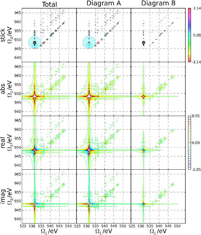
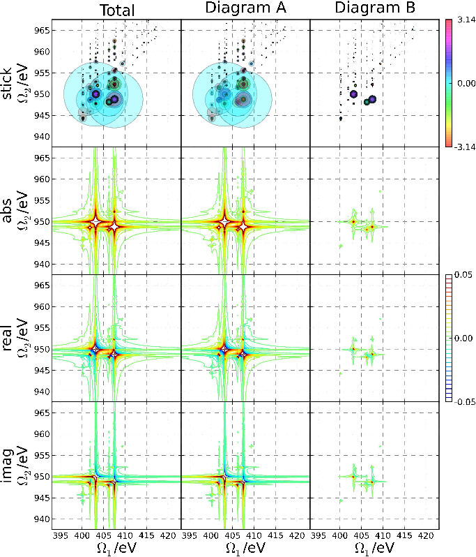


To better illustrate the relationship between the 2D-XDQC signal and the linear absorption, we display the ONNO and NONO signals with the XANES marginals in Fig. 7. We shift the N1s and O1s XANES on the axis to match the strongest features. If the core excitations were uncoupled, the peaks in for a fixed should reproduce the XANES of the core resonant with the second pulse, with one peak quenched due to Pauli repulsion with the previously excited core-electron. This might explain the strong diagonal character of the ONNO signal, in which the strong peak A is repeated for increasing . This interpretation does not hold for the NONO signal, with its group of four strong peaks around eV and eV. The pattern does not match a shifted XANES signal, implying strong correlations in the DCESs. Comparing the linear absorption (Fig. 4) to the ONNO XDQC signal for 5fs (Fig. 5), we find one medium and two stronger features in the nitrogen K-edge XANES, and one strong, two weak and one medium intense features for oxygen K-edge XANES. The corresponding peaks are marked as , A, B , C, E, F, D in Fig. 4. The N and O K-edge XANES are well described by a single particle picture. The dominant particle MOs in the CI expansions of these SCESs are shown on Fig. 8.
In the ideal zero-DCES-SCES correlation case we expect to see two parallel lines of strong features in Fig. 5 corresponding to A and B in the nitrogen XANES, but we only see one clear set of “diagonal” resonances. The peaks corresponding to states E and F in the oxygen XANES are much weaker than that of D, but their corresponding peaks in the XDQC spectra (in Fig. 5) are as strong as as that of D. State E shares the same particle MO as that of , implying a strong coupling between E and , which explains the corresponding strong XDQC signal. But for the XDQC peak corresponding to F, it is very difficult to compare the coupling strength of F and to that of D and , simply by their dominant particle MOs. Even the calculated energy of the DCES is close to the sum of two single excitations, the wavefunction is not the simple outer product of two SCES wavefunctions. The single particle picture can not explain why the XDQC peak corresponding to F also becomes strong, suggesting that many-body effects dominate the signal.
As discussed in Sec. II, the DCES () strongly depend on the order of core excitation by the first two pulses, showing that XDQC is sensitive to the order of the formation of doubly core-excited states. Our XDQC simulations also show large differences between the two protocols explained in the following, reflecting the approximate treatment of many-body effects. In Figs. 5 and 6 we assumed the states were relaxed in the field of the first (core hole a), and calculated using response theory with respect to the second excited core (core hole b, protocol i). In Fig. 9 we present an example of the opposite protocol for the ONNO technique: the states are generated using SCF relaxation for core hole b and then response theory for core hole a (protocol ii). We observe a different blurred line pattern in the spectra obtained with protocol ii (see Fig. 9). Different levels of theory show a different type of DCES-SCES correlation. The protocol i diagram A signal also shows a stronger diagonal component than the corresponding protocol ii signal, which displays a different density of two-particle states on the axis. Comparing XDQC signals from different pulse orders with experiments should reveal how well those theories treat the very specific correlation between a DCES and SCES. This could be valuable in future methodology development for DCESs.
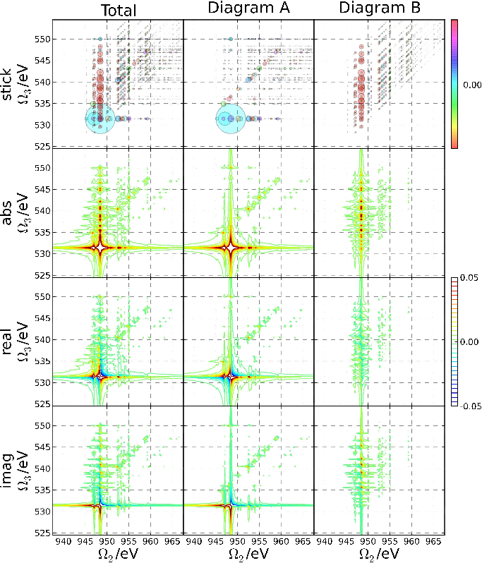
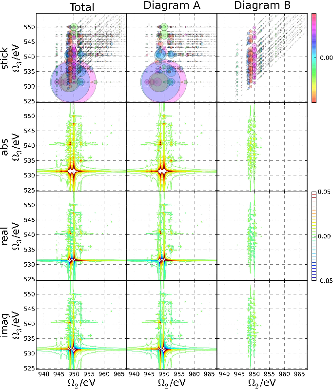
Another portion of the signal, , is shown in Figs. 10 and 11. In these graphs, resonances along correspond to doubly excited states (), and shows the final single excited states ( and ) in the XDQC process. As with the signals, there are diagonal characteristics in the ONNO spectra (Fig. 10) which are absent in the NONO spectra (Fig. 11). This is further evidence for the increased correlations for the states probed by the ONNO process. In the signal the resonances for both A and B diagrams are the same, only the phases for two contributions differ. The signal has qualitatively different peaks along for the two diagrams, as expected, since these diagrams differ in this time period.
VII Conclusions
Typically the overlaps of valence holes or electron orbitals are higher than those of core holes or electrons. The correlations between valence excitations are stronger than those between core excitations, which makes the corresponding DQC signals more complicated than those in the present work.[137] We have demonstrated qualitative differences in the stimulated XDQC signals depending on the order of core-excitations at different elements in a small organic molecule. As an experimental technique, XDQC may be used to fingerprint different theoretical approaches for modeling core-excitation, by dissecting dynamical doubly-core-excited resonances corresponding to the effects of valence relaxation induced by the core hole. Additional work will be required to further analyze the spectra reported here. First, a detailed description of the valence dynamics, and a comparison of the TDDFT theory with the more easily interpreted orbital theory should highlight the effect of electron correlation on the XDQC signal. Second, with a higher level of theory to describe DCESs, the variation of the resonances with can be used to measure how the order of core-excitation affects the two-particle density of states. The core hole has a unit charge which creates a very strong field over atomic length scales. If the delay between the first two pulses is varied, the changes in the resonances along will reflect the order of perturbation theory necessary to correctly model this strong interaction with the valence band. For short , linear response theory alone, or supplemented with a full or partial core hole orbital transformation may adequately capture this effect, as it does in linear absorption. We demonstrated significant differences between the XDQC signals predicted by the calculation protocols. Interpolation between the extremes of linear response (first order), and a full SCF calculation will require a higher level of theory to describe many-body effects in the core-excitation.
In the simulations presented here the relaxation of single and double core-excited states, is treated phenomenologically. We only include population decay through Auger or a radiative process that destroys the core hole. We further use the same decay rate for all SCESs and DCESs, independent of the orbitals involved. Interaction of the system with a bath, composed of vibrational and valence-electron degrees of freedom, could introduce additional pure dephasing. Nonlinear spectroscopy has been successful in lower frequency regimes (NMR to the visible) at disentangling different underlying mechanisms for excited state decay and dephasing.[138] Similar effects are expected in core-excitation spectra. Estimating their magnitude, comparing them to population decay rates, and designing experiments that distinguish between them is an interesting future topic. One manifestation of these effects in existing X-ray experiments are fluorescence vs. Raman signals, which are controlled by the ratio of pure dephasing and population relaxation rates.
Acknowledgements.
We gratefully acknowledge the support of the Chemical Sciences, Geosciences and Biosciences Division, Office of Basic Energy Sciences, Office of Science, U.S. Department of Energy, the support of the National Science Foundation (NSF) through Grant No. CHE-1058791 and the National Institute of Health (Grant GM-59230). Help on the REW-TDDFT calculations from Niranjan Govind of the Pacific Northwest National Lab (PNNL) is greatly appreciated.Appendix A Orientational Tensor Averaging
The dipole and electric field polarization tensor contributions to the signal must be rotationally averaged over all possible orientations of the molecule. The rotationally averaged[139] signal is
| (13) |
where , is the the polarization of the th pulse polarization vector, and represent various contractions over the tensor components of the response;
| (14) |
| (15) |
and
| (16) |
For the all parallel pulse configuration, the signal is proportional to the sum of all three
| (17) |
References
- [1] T. Popmintchev, M.-C. Chen, P. Arpin, M. M. Murnane, and H. C. Kapteyn, Nat. Photonics 4, 822 (2010).
- [2] F. Krausz and M. Ivanov, Rev. Mod. Phys. 81, 163 (2009).
- [3] P. Emma, R. Akre, J. Arthur, R. Bionta, C. Bostedt, J. Bozek, A. Brachmann, P. Bucksbaum, R. Coffee, F.-J. Decker, Y. Ding, D. Dowell, S. Edstrom, A. Fisher, J. Frisch, S. Gilevich, J. Hastings, G. Hays, P. Hering, Z. Huang, R. Iverson, H. Loos, M. Messerschmidt, A. Miahnahri, S. Moeller, H.-D. Nuhn, G. Pile, D. Ratner, J. Rzepiela, D. Schultz, T. Smith, P. Stefan, H. Tompkins, J. Turner, J. Welch, W. White, J. Wu, G. Yocky, and J. Galayda, Nat. Photonics 4, 641 (2010).
- [4] J. Ullrich, A. Rudenko, and R. Moshammer, Ann. Rev. Phys. Chem. 63, 635 (2012).
- [5] L. Young, E. P. Kanter, B. Krässig, Y. Li, A. M. March, S. T. Pratt, R. Santra, S. H. Southworth, N. Rohringer, L. F. DiMauro, G. Doumy, C. A. Roedig, N. Berrah, L. Fang, M. Hoener, P. H. Bucksbaum, J. P. Cryan, S. Ghimire, J. M. Glownia, D. A. Reis, J. D. Bozek, C. Bostedt, and M. Messerschmidt, Nature 466, 56 (2010).
- [6] M. Hoener, L. Fang, O. Kornilov, O. Gessner, S. T. Pratt, M. Gühr, E. P. Kanter, C. Blaga, C. Bostedt, J. D. Bozek, P. H. Bucksbaum, C. Buth, M. Chen, R. Coffee, J. Cryan, L. DiMauro, M. Glownia, E. Hosler, E. Kukk, S. R. Leone, B. McFarland, M. Messerschmidt, B. Murphy, V. Petrovic, D. Rolles, and N. Berrah, Phys. Rev. Lett. 104, 253002 (2010).
- [7] P. Elliott, S. Goldson, C. Canahui, and N. T. Maitra, Chem. Phys. 391, 110 (2011).
- [8] J.-P. Connerade, Highly Excited Atoms (Cambridge University Press, 1998).
- [9] R. Santra, N. V. Kryzhevoi, and L. S. Cederbaum, Phys. Rev. Lett. 103, 013002 (2009a).
- [10] K. Ueda and O. Takahashi, J. Electron. Spectrosc. Relat. Phenom. 185, 301 (2012).
- [11] N. V. Kryzhevoi, R. Santra, and L. S. Cederbaum, J. Chem. Phys. 135, 084302 (2011a).
- [12] P. Salén, P. van der Meulen, H. T. Schmidt, R. D. Thomas, M. Larsson, R. Feifel, M. N. Piancastelli, L. Fang, B. Murphy, T. Osipov, N. Berrah, E. Kukk, K. Ueda, J. D. Bozek, C. Bostedt, S. Wada, R. Richter, V. Feyer, and K. C. Prince, Phys. Rev. Lett. 108, 153003 (2012).
- [13] M. Tashiro, K. Ueda, and M. Ehara, Chem. Phys. Lett. 521, 45 (2012).
- [14] J. Kim, S. Mukamel, and G. D. Scholes, Acc. Chem. Res. 42, 1375 (2009).
- [15] S. Mukamel, R. Oszwałdowski, and D. Abramavicius, Phys. Rev. B 75, 245305 (2007a).
- [16] W. Zhuang, D. Abramavicius, and S. Mukamel, Proc. Natl. Acad. Sci. 102, 7443 (2005).
- [17] A. Nemeth, F. Milota, T. Mančal, T. Pullerits, J. Sperling, J. Hauer, H. F. Kauffmann, and N. Christensson, J. Chem. Phys. 133, 094505 (2010).
- [18] S. Mukamel, R. Oszwałdowski, and L. Yang, J. Chem. Phys. 127, 221105 (2007b).
- [19] D. Karaiskaj, A. D. Bristow, L. Yang, X. Dai, R. P. Mirin, S. Mukamel, and S. T. Cundiff, Phys. Rev. Lett. 104, 117401 (2010).
- [20] K. W. Stone, K. Gundogdu, D. B. Turner, X. Li, S. T. Cundiff, and K. A. Nelson, Science 324, 1169 (2009).
- [21] X. Dai, M. Richter, H. Li, A. D. Bristow, C. Falvo, S. Mukamel, and S. T. Cundiff, Phys. Rev. Lett. 108, 193201 (2012).
- [22] J. Orenstein, Phys. Today 65, 44 (2012).
- [23] G. D. Mahan, Condensed Matter in a Nutshell (Princeton University Press, 2011).
- [24] D. Fausti, R. I. Tobey, N. Dean, S. Kaiser, A. Dienst, M. C. Hoffmann, S. Pyon, T. Takayama, H. Takagi, and A. Cavalleri, Science 331, 189 (2011).
- [25] I. V. Schweigert and S. Mukamel, Phys. Rev. A 78, 052509 (2008a).
- [26] M. Stener, G. Fronzoni, and M. de Simone, Chem. Phys. Lett. 373, 115 (2003).
- [27] N. A. Besley and A. Noble, J. Phys. Chem. C 111, 3333 (2007).
- [28] S. DeBeer-George, T. Petrenko, and F. Neese, J. Phys. Chem. A 112, 12936 (2008).
- [29] N. A. Besley, M. J. G. Peach, and D. J. Tozer, Phys. Chem. Chem. Phys. 11, 10350 (2009).
- [30] N. A. Besley and F. A. Asmuruf, Phys. Chem. Chem. Phys. 12, 12024 (2010).
- [31] W. Liang, S. A. Fischer, M. J. Frisch, and X. Li, J. Chem. Theory Comput. 7, 3540 (2011).
- [32] K. Lopata, B. E. V. Kuiken, M. Khalil, and N. Govind, J. Chem. Theory Comput. 8, 3284 (2012).
- [33] Y. Zhang, J. D. Biggs, D. Healion, N. Govind, and S. Mukamel, J. Chem. Phys. 137, 194306 (2012).
- [34] N. Ottosson, E. F. Aziz, H. Bergersen, W. Pokapanich, G. Öhrwall, S. Svensson, W. Eberhardt, and O. Björneholm, J. Phys. Chem. B 112, 16642 (2008a).
- [35] N. Ottosson, E. F. Aziz, I. L. Bradeanu, S. Legendre, G. Öhrwall, S. Svensson, O. Björneholm, and W. Eberhardt, Chem. Phys. Lett. 460, 540 (2008b).
- [36] H. Ikeura-Sekiguchi, T. Sekiguchi, Y. Kitajima, and Y. Baba, App. Surf. Sci. 169-170, 282 (2001).
- [37] D. P. Chong, J. Electron. Spectrosc. Relat. Phenom. 184, 164 (2011).
- [38] H. Ågren and H. J. A. Jensen, Chem. Phys. 172, 45 (1993).
- [39] O. Takahashi, M. Tashiro, M. Ehara, K. Yamasaki, and K. Ueda, Chem. Phys. 384, 28 (2011a).
- [40] J. Jadżyn and J. Świergiel, Phys. Chem. Chem. Phys. 14, 3170 (2012).
- [41] Y. L. Li, L. Huang, R. J. Dwayne Miller, T. Hasegawa, and Y. Tanimura, J. Chem. Phys. 128, 234507 (2008a).
- [42] A. Paarmann, M. Lima, R. Chelli, V. V. Volkov, R. Righini, and R. J. D. Miller, Phys. Chem. Chem. Phys. 13, 11351 (2011).
- [43] J. Jortner and S. A. Rice, J. Chem. Phys. 44, 3364 (1966).
- [44] D. Sangalli, P. Romaniello, G. Onida, and A. Marini, J. Chem. Phys. 134, 034115 (2011).
- [45] L. Serrano-Andres, M. Merchan, I. Nebot-Gil, R. Lindh, and B. O. Roos, J. Chem. Phys. 98, 3151 (1993).
- [46] K. N. amd Haruyuki Nakano and K. Hirao, Int. J. Quantum Chem. 66, 157 (1998).
- [47] C. Hsu, S. Hirata, and M. Head-Gordon, J. Phys. Chem. A 105, 451 (2001).
- [48] J. H. Starcke, M. Wormit, J. Schirmer, and A. Dreuw, Chem. Phys. 329, 39 (2006).
- [49] J. H. Starcke, M. Wormit, and A. Dreuw, J. Chem. Phys. 131, 144311 (2009).
- [50] S. Knippenberg, J. H. Starcke, M. Wormit, and A. Dreuw, Mol. Phys. 108, 2801 (2010).
- [51] C. Angeli and M. Pastore, J. Chem. Phys. 134, 184302 (2011).
- [52] M. Schmidt and P. Tavan, J. Chem. Phys. 136, 124309 (2012).
- [53] E. Otero, N. Kosugi, and S. G. Urguhart, J. Chem. Phys. 131, 114313 (2009).
- [54] M. E. Casida, J. Chem. Phys. 122, 054111 (2005).
- [55] M. Casida, A. Ipatov, and F. Cordova, in Time-Dependent Density Functional Theory, Lecture Notes in Physics, Vol. 706, edited by M. A. Marques, C. A. Ullrich, F. Nogueira, A. Rubio, K. Burke, and E. K. U. Gross (Spinger-Verlag Berlin Heidelberg, 2006) Chap. 16, p. 243.
- [56] P. Th. van Duijnen, S. N. Greene, and N. G. J. Richards, J. Chem. Phys. 127, 045105 (2007).
- [57] Z. Li and W. Liu, J. Chem. Phys. 133, 064106 (2010).
- [58] Y. Kurashige, H. Nakano, Y. Nakao, and K. Hirao, Chem. Phys. Lett. 400, 425 (2004).
- [59] V. Carravetta and H. Ågren, in Computational Strategies for Spectroscopy, edited by V. Barone (John Wiley & Sons, Inc.,, 2011) p. 137205.
- [60] O. Lehtonen, D. Sundholm, R. Send, and M. P. Johansson, J. Chem. Phys. 131, 024301 (2009).
- [61] C. M. Marian and N. Gilka, J. Chem. Theory Comput. 4, 1501 (2008).
- [62] I. A. Mikhailov, S. Tafur, and A. E. Masunov, Phys. Rev. A 77, 012510 (2008).
- [63] M. A. Marques, C. A. Ullrich, F. Nogueira, A. Rubio, K. Burke, and E. K. U. Gross, eds., Time-dependent Density Functional Theory (Springer, 2006).
- [64] C. A. Ullrich, Time-dependent Density Functional Theory: Concepts and Applications (Oxford University Press, USA, 2012).
- [65] N. T. Maitra, F. Zhang, R. J. Cave, and K. Burke, J. Chem. Phys. 120, 5932 (2004).
- [66] S. Tretiak, V. Chernyak, and S. Mukamel, Int. J. Quantum Chem. 70, 711 (1998).
- [67] S. Tretiak and V. Chernyak, J. Chem. Phys. 119, 8809 (2003).
- [68] E. K. U. Gross, J. F. Dobson, and M. Petersilka, in Density-Functional Theory II, Topics in Current Chemistry, Vol. 181, edited by R. F. Nalewajski (Spinger, Berlin, 1996) p. 81.
- [69] S. Hirata and M. Head-Gordon, Chem. Phys. Lett. 314, 291 (1999).
- [70] R. J. Cave, F. Zhang, N. T. Maitra, and K. Burke, Chem. Phys. Lett. 389, 39 (2004).
- [71] G. Mazur and R. Włodarczyk, J. Comput. Chem. 30, 811 (2009).
- [72] G. Mazur, M. Makowski, R. Włodarczyk, and Y. Aoki, Int. J. Quant. Chem. 111, 819 (2011).
- [73] M. Huix-Rotllant, A. Ipatov, A. Rubio, and M. E. Casida, Chem. Phys. 391, 120 (2011).
- [74] P. Romaniello, D. Sangalli, J. A. Berger, F. Sottile, L. G. Molinari, L. Reining, and G. Onida, J. Chem. Phys. 130, 044108 (2009).
- [75] A. I. Krylov, Chem. Phys. Lett. 338, 375 (2001a).
- [76] A. I. Krylov, Chem. Phys. Lett. 350, 522 (2001b).
- [77] A. I. Krylov and C. D. Sherrill, J. Chem. Phys. 116, 3194 (2002).
- [78] L. V. Slipchenko and A. I. Krylov, J. Chem. Phys. 117, 3694 (2002).
- [79] Y. Shao, M. Head-Gordon, and A. I. Krylov, J. Chem. Phys. 118, 4807 (2003).
- [80] F. Wang and T. Ziegler, J. Chem. Phys. 121, 12191 (2004).
- [81] Z. Rinkevicius, O. Vahtras, and H. Ågren, J. Chem. Phys. 133, 114104 (2010).
- [82] N. Minezawa and M. S. Gordon, J. Phys. Chem. A 115, 7901 (2011).
- [83] Z. Li and W. Liu, J. Chem. Phys. 136, 024107 (2012).
- [84] Y. A. Bernard, Y. Shao, and A. I. Krylov, J. Chem. Phys. 136, 204103 (2012).
- [85] C. M. Isborn and X. Li, J. Chem. Phys. 129, 204107 (2008).
- [86] W. Liang, C. M. Isborn, and X. Li, J. Chem. Phys. 131, 204101 (2009).
- [87] V. N. Glushkov and X. Assfeld, J. Chem. Phys. 132, 204106 (2010).
- [88] V. N. Glushkov and X. Assfeld, J. Comput. Chem. 33, 2058 (2012).
- [89] K. J. H. Giesbertz, E. J. Baerends, and O. V. Gritsenko, Phys. Rev. Lett. 101, 033004 (2008).
- [90] P. Nozieres and C. T. D. Dominicis, Phys. Rev. 178, 1097 (1969).
- [91] W. H. E. Schwarz and R. J. Buenker, Chem. Phys. 13, 153 (1976).
- [92] I. V. Schweigert and S. Mukamel, Phys. Rev. Lett. 99, 163001 (2007a).
- [93] I. V. Schweigert and S. Mukamel, Phys. Rev. A 76, 012504 (2007b).
- [94] I. V. Schweigert and S. Mukamel, J. Chem. Phys. 128, 184307 (2008b).
- [95] I. V. Schweigert and S. Mukamel, Phys. Rev. A 78, 052509 (2008c).
- [96] D. M. Healion, I. V. Schweigert, and S. Mukamel, J. Phys. Chem. A 112, 11449 (2008).
- [97] M. N. R. Wohlfarth and L. S. Cederbaum, J. Chem. Phys. 116, 8723 (2002).
- [98] M. Cavalleri, M. Odelius, D. Nordlund, A. Nilsson, and L. G. Pettersson, Phys. Chem. Chem. Phys. 15, 2854 (2005).
- [99] H. Ågren, V. Carravetta, O. Vahtras, and L. G. M. Pettersson, Chem. Phys. Lett. 222, 75 (1994).
- [100] H. Ågren, V. Carravetta, O. Vahtras, and L. G. M. Pettersson, Theor. Chem. Acta 97, 14 (1997).
- [101] W. J. Hunt and W. A. Goddard III, Chem. Phys. Lett. 3, 414 (1969).
- [102] D. Healion, H. Wang, and S. Mukamel, J. Chem. Phys. 134, 124101 (2011).
- [103] J. D. Biggs, Y. Zhang, D. Healion, and S. Mukamel, J. Chem. Phys. 136, 174117 (2012a).
- [104] J. H. D. Eland, M. Tashiro, P. Linusson, M. Ehara, K. Ueda, and R. Feifel, Phys. Rev. Lett. 105, 213005 (2010).
- [105] N. V. Kryzhevoi, R. Santra, and L. S. Cederbaum, J. Chem. Phys. 135, 084302 (2011b).
- [106] L. Inhester, C. F. Burmeister, G. Groenhof, and H. Grubmüller, J. Chem. Phys. 136, 144304 (2012).
- [107] R. Santra, N. V. Kryzhevoi, and L. S. Cederbaum, Phys. Rev. Lett. 103, 013002 (2009b).
- [108] J. Schirmer, L. S. Cederbaum, and O. Walter, Phys. Rev. A 28, 1237 (1983).
- [109] J. Schirmer and A. Barth, Z. Phys. A 317, 267 (1984).
- [110] J. Niskanen, P. Norman, H. Aksela, and H. Ågren, J. Chem. Phys. 135, 054310 (2011).
- [111] O. Takahashi, M. Tashiro, M. Ehara, K. Yamasaki, and K. Ueda, J. Phys. Chem. A 115, 12070 (2011b).
- [112] O. Takahashi, K. Yamasaki, S. Nagaoka, and K. Ueda, Chem. Phys. Lett. 518, 44 (2011c).
- [113] A. T. B. Gilbert, N. A. Besley, and P. M. W. Gill, J. Phys. Chem. A 112, 13164 (2008).
- [114] U. Ekström, P. Norman, V. Carravetta, and H. Ågren, Phys. Rev. Lett. 97, 143001 (2006).
- [115] M. Linares, S. Stafström, Z. Rinkevicius, H. Ågren, and P. Norman, J. Phys. Chem. B 115, 5096 (2011).
- [116] B. Brena, P. E. M. Siegbahn, and H. Ågren, J. Am. Chem. Soc. 134, 17157 (2012).
- [117] A. Nardelli, G. Fronzoni, and M. Stener, Phys. Chem. Chem. Phys. 13, 480 (2011).
- [118] J. P. Perdew and A. Zunger, Phys. Rev. B 23, 5048 (1981).
- [119] G. Tu, Z. Rinkevicius, O. Vahtras, H. Ågren, U. Ekström, P. Norman, and V. Carravetta, Phys. Rev. A 76, 022506 (2007).
- [120] A. Nakata, Y. Imamura, T. Ostuka, and H. Nakai, J. Chem. Phys. 124, 194105 (2006a).
- [121] A. Nakata, Y. Imamura, and H. Nakai, J. Chem. Phys. 125, 064109 (2006b).
- [122] Y. Imamura, R. Kobayashi, and H. Nakai, J. Chem. Phys. 134, 124113 (2011).
- [123] J.-W. Song, M. A. Watson, A. Nakata, and K. Hirao, J. Chem. Phys. 129, 184113 (2008).
- [124] D. Prendergast and G. Galli, Phys. Rev. Lett. 96, 215502 (2006).
- [125] M. Taillefumier, D. Cabaret, A.-M. Flank, and F. Mauri, Phys. Rev. B 66, 195107 (2002).
- [126] A. Ipatov, F. Cordova, L. J. Doriol, and M. E. Casida, J. Mol. Struct.: THEOCHEM 914, 60 (2009).
- [127] Z. Li, W. Liu, Y. Zhang, and B. Suo, J. Chem. Phys. 134, 134101 (2011).
- [128] Z. Li and W. Liu, J. Chem. Phys. 135, 194106 (2011).
- [129] I. V. Schweigert and S. Mukamel, Phys. Rev. A 77, 033802 (2008d).
- [130] J. D. Biggs, J. A. Voll, and S. Mukamel, Phil. Trans. R. Soc. A 370, 3709 (2012b).
- [131] O. Roslyak, B. Fingerhut, K. Bennet, and S. Mukamel, (Submitted, 2012).
- [132] A. D. Becke, J. Chem. Phys. 98, 5648 (1993).
- [133] P. Stephens, F. Devlin, C. Chabalowski, and M. Frisch, J. Phys. Chem. 98, 11623 (1994).
- [134] T. H. Dunning, J. Chem. Phys. 90, 1007 (1989).
- [135] M. Valiev, E. Bylaska, N. Govind, K. Kowalski, T. Straatsma, H. van Dam, D. Wang, J. Nieplocha, E. Apra, T. Windus, and W. de Jong, Comput. Phys. Commun. 181, 1477 (2010).
- [136] J. Stöhr, NEXAFS Spectroscopy (Springer-Verlag, 1992) pp. 34–39.
- [137] Z. Li, D. Abramavicius, and S. Mukamel, J. Am. Chem. Soc. 130, 3509 (2008b).
- [138] S. Mukamel, Principles of Nonlinear Optical Spectroscopy (Oxford University Press, USA, 1999).
- [139] D. L. Andrews and T. Thirunamachandran, J. Chem. Phys. 67, 5026 (1977).
- [140] M. Robin, I. Ishii, R. McLaren, and A. Hitchcock, J. Electron. Spectrosc. Relat. Phenom. 47, 53 (1988).