Load balancing of dynamical distribution networks with flow constraints and unknown in/outflows
Abstract
We consider a basic model of a dynamical distribution network, modeled as a directed graph with storage variables corresponding to every vertex and flow inputs corresponding to every edge, subject to unknown but constant inflows and outflows. As a preparatory result it is shown how a distributed proportional-integral controller structure, associating with every edge of the graph a controller state, will regulate the state variables of the vertices, irrespective of the unknown constant inflows and outflows, in the sense that the storage variables converge to the same value (load balancing or consensus). This will be proved by identifying the closed-loop system as a port-Hamiltonian system, and modifying the Hamiltonian function into a Lyapunov function, dependent on the value of the vector of constant inflows and outflows. In the main part of the paper the same problem will be addressed for the case that the input flow variables are constrained to take value in an interval. We will derive sufficient and necessary conditions for load balancing, which only depend on the structure of the network in relation with the flow constraints.
Keywords:
PI controllers , flow constraints , directed graphs , port-Hamiltonian systems , consensus algorithms , Lyapunov stability1 Introduction
In this paper we study a basic model for the dynamics of a distribution network. Identifying the network with a directed graph we associate with every vertex of the graph a state variable corresponding to storage, and with every edge a control input variable corresponding to flow, which is constrained to take value in a given closed interval. Furthermore, some of the vertices serve as terminals where an unknown but constant flow may enter or leave the network in such a way that the total sum of inflows and outflows is equal to zero. The control problem to be studied is to derive necessary and sufficient conditions for a distributed control structure (the control input corresponding to a given edge only depending on the difference of the state variables of the adjacent vertices) which will ensure that the state variables associated to all vertices will converge to the same value equal to the average of the initial condition, irrespective of the values of the constant unknown inflows and outflows.
The structure of the paper is as follows. Some preliminaries and notations will be given in Section 2. In Section 3 we will show how in the absence of constraints on the flow input variables a distributed proportional-integral (PI) controller structure, associating with every edge of the graph a controller state, will solve the problem if and only if the graph is weakly connected. This will be shown by identifying the closed-loop system as a port-Hamiltonian system, with state variables associated both to the vertices and the edges of the graph, in line with the general definition of port-Hamiltonian systems on graphs [1, 2, 3, 4]; see also [5, 6]. The proof of asymptotic load balancing will be given by modifying, depending on the vector of constant inflows and outflows, the total Hamiltonian function into a Lyapunov function. In examples the obtained PI-controller often has a clear physical interpretation, emulating the physical action of adding energy storage and damping to the edges.
The main contribution of the paper resides in Sections 4 and 5, where the same problem is addressed for the case of constraints on the flow input variables. In Section 4 it will be shown that in the case of zero inflow and outflow the state variables of the vertices converge to the same value if and only if the network is strongly connected. This will be shown by constructing a Lyapunov function based on the total Hamiltonian and the constraint values. This same construction will be extended in Section 5 to the case of non-zero inflows and outflows, leading to the result that in this case asymptotic load balancing is reached if and only the graph is not only strongly connected but also balanced. Finally, Section 6 contains the conclusions.
Some preliminary results, in particular concerning Section 3, have been already reported before in [7].
2 Preliminaries and notations
First we recall some standard definitions regarding directed graphs, as can be found e.g. in [8]. A directed graph consists of a finite set of vertices and a finite set of edges, together with a mapping from to the set of ordered pairs of , where no self-loops are allowed. Thus to any edge there corresponds an ordered pair (with ), representing the tail vertex and the head vertex of this edge.
A directed graph is completely specified by its incidence matrix , which is an matrix, being the number of vertices and being the number of edges, with element equal to if the edge is towards vertex , and equal to if the edge is originating from vertex , and otherwise. Since we will only consider directed graphs in this paper ‘graph’ will throughout mean ‘directed graph’ in the sequel. A directed graph is strongly connected if it is possible to reach any vertex starting from any other vertex by traversing edges following their directions. A directed graph is called weakly connected if it is possible to reach any vertex from every other vertex using the edges not taking into account their direction. A graph is weakly connected if and only if . Here denotes the -dimensional vector with all elements equal to . A graph that is not weakly connected falls apart into a number of weakly connected subgraphs, called the connected components. The number of connected components is equal to . For each vertex, the number of incoming edges is called the in-degree of the vertex and the number of outgoing edges its out-degree. A graph is called balanced if and only if the in-degree and out-degree of every vertex are equal. A graph is balanced if and only if .
Given a graph, we define its vertex space as the vector space of all functions from to some linear space . In the rest of this paper we will take for simplicity , in which case the vertex space can be identified with . Similarly, we define its edge space as the vector space of all functions from to , which can be identified with . In this way, the incidence matrix of the graph can be also regarded as the matrix representation of a linear map from the edge space to the vertex space .
Notation: For the notation will denote elementwise inequality . For the multidimensional saturation function is defined as
| (1) |
3 A dynamic network model with PI controller
Let us consider the following dynamical system defined on the graph
| (2) |
where is any differentiable function, and denotes the column vector of partial derivatives of . Here the element of the state vector is the state variable associated to the vertex, while is a flow input variable associated to the edge of the graph. System (2) defines a port-Hamiltonian system ([9, 10]), satisfying the energy-balance
| (3) |
Note that geometrically its state space is the vertex space, its input space is the edge space, while its output space is the dual of the edge space.
Example 3.1 (Hydraulic network).
Consider a hydraulic network, modeled as a directed graph with vertices (nodes) corresponding to reservoirs, and edges (branches) corresponding to pipes. Let be the stored water at vertex , and the flow through edge . Then the mass-balance of the network is summarized in
| (4) |
where is the incidence matrix of the graph. Let furthermore denote the stored energy in the reservoirs (e.g., gravitational energy). Then are the pressures at the vertices, and the output vector is the vector whose element is the pressure difference across the edge linking vertex to vertex .
As a next step we will extend the dynamical system (2) with a vector of inflows and outflows
| (5) |
with an matrix whose columns consist of exactly one entry equal to (inflow) or (outflow), while the rest of the elements is zero. Thus specifies the terminal vertices where flows can enter or leave the network.
In this paper we will regard as a vector of constant disturbances, and we want to investigate control schemes which ensure asymptotic load balancing of the state vector irrespective of the (unknown) disturbance . The simplest control possibility is to apply a proportional output feedback
| (6) |
where is a diagonal matrix with strictly positive diagonal elements . Note that this defines a decentralized control scheme if is of the form , in which case the input is given as times the difference of the component of corresponding to the head vertex of the edge and the component of corresponding to its tail vertex. This control scheme leads to the closed-loop system
| (7) |
In case of zero in/outflows this implies the energy-balance
| (8) |
Hence if is radially unbounded it follows that the system trajectories of the closed-loop system (7) will converge to the set
| (9) |
and thus to the load balancing set
if and only if , or equivalently [8], if and only if the graph is weakly connected.
In particular, for the standard Hamiltonian this means that the state variables converge to a common value as . Since it follows that this common value is given as .
For proportional control will not be sufficient to reach load balancing, since the disturbance can only be attenuated at the expense of increasing the gains in the matrix . Hence we consider proportional-integral (PI) control given by the dynamic output feedback
| (10) |
where denotes the storage function (energy) of the controller. Note that this PI controller is of the same decentralized nature as the static output feedback .
The element of the controller state can be regarded as an additional state variable corresponding to the edge. Thus , the edge space of the network. The closed-loop system resulting from the PI control (10) is given as
| (11) |
This is again a port-Hamiltonian system11 1 See [1, 2, 3, 4] for a general definition of port-Hamiltonian systems on graphs., with total Hamiltonian , and satisfying the energy-balance
| (12) |
Consider now a constant disturbance for which there exists a matching controller state , i.e.,
| (13) |
This allows us to modify the total Hamiltonian into22 2 This function was introduced for passive systems with constant inputs in [11].
| (14) |
which will serve as a candidate Lyapunov function; leading to the following theorem.
Theorem 1.
Consider the system (5) on the graph in closed loop with the PI-controller (10). Let the constant disturbance be such that there exists a satisfying the matching equation (13). Assume that is radially unbounded. Then the trajectories of the closed-loop system (11) will converge to an element of the load balancing set
| (15) |
if and only if is weakly connected.
Proof.
Suppose is weakly connected. By (12) for we obtain, making use of (13),
| (16) | ||||
Hence by LaSalle’s invariance principle the system trajectories converge to the largest invariant set contained in
Substitution of in the closed-loop system equations (11) yields constant and . Since the graph is weakly connected implies . If the graph is not weakly connected then the above analysis will hold on every connected component, but the common value will be different for different components. ∎
Corollary 2.
Corollary 3.
In case of the standard quadratic Hamiltonians , there exists for every a controller state such that (13) holds if and only if
| (17) |
Furthermore, in this case equals the radially unbounded function , while convergence will be towards the load balancing set .
A necessary (and in case the graph is weakly connected necessary and sufficient) condition for the inclusion is that . In its turn is equivalent to the fact that for every the total inflow into the network equals to the total outflow). The condition also implies
| (18) |
implying (as in the case ) that is a conserved quantity for the closed-loop system (11). In particular it follows that the limit value is determined by the initial condition .
Example 3.2 (Hydraulic network continued).
The proportional part of the controller corresponds to adding damping to the dynamics (proportional to the pressure differences along the edges). The integral part of the controller has the interpretation of adding compressibility to the hydraulic network dynamics. Using this emulated compressibility, the PI-controller is able to regulate the hydraulic network to a load balancing situation where all pressures are equal, irrespective of the constant inflow and outflow satisfying the matching condition (13). Note that for the Hamiltonian the pressures are equal to each other if and only if the water levels are equal.
4 Constrained flows: the case without in/out flows
In many cases of interest, the elements of the vector of flow inputs corresponding to the edges of the graph will be constrained, that is
| (19) |
for certain vectors and satisfying (throughout denotes element-wise inequality). This leads to the following constrained version33 3 See also [12] for a related problem setting where a constrained version of the proportional controller (6) is considered. of the PI controller (10) given in the previous section
| (20) |
Throughout this paper we make the following assumption on the flow constraints.
Assumption 4.
| (21) |
It is important to note that we may change the orientation of some of the edges of the graph at will; replacing the corresponding columns of the incidence matrix by . Noting the identity this implies that we may assume without loss of generality that the orientation of the graph is chosen such that
| (22) |
This will be assumed throughout the rest of the paper. In general, we will say that any orientation of the graph is compatible with the flow constraints if (22) holds. If the -th edge is such that then we will call this edge an uni-directional edge, while if then the edge is called a bi-directional edge.
In this section we will first analyze the closed-loop system for the constrained PI-controller under the simplifying assumption of zero inflow and outflow (). In the next section we will deal with the general case. Furthermore, for simplicity of exposition we consider throughout the rest of this paper the standard Hamiltonian for the constrained PI controller and the identity gain matrix , while we also throughout assume that the Hessian matrix of Hamiltonian is positive definite for any . Thus we consider the closed-loop system
| (23) |
In order to state the main theorem of this section we need one more definition concerning strong connectedness with respect to flow constraints.
Definition 5.
Consider the directed graph together with the constraint values satisfying (22). Then we will call the graph strongly connected with respect to the flow constraints if the following holds: for every two vertices there exists an orientation of the graph compatible with the flow constraints44 4 Note that for different pairs of vertices we may need different orientations compatible with the flow constraints. Thus the definition of strong connectedness with respect to the flow constraints is weaker than the existence of an orientation of the graph compatible with the flow constraints in which the graph is strongly connected. and a directed path (directed with respect to this orientation) from to .
Theorem 6.
Consider the closed-loop system on a graph with flow constraints satisfying (22). Then its solutions converge to the load balancing set
| (24) |
if and only if the graph is strongly connected with respect to the flow constraints.
Proof.
Sufficiency: Consider the Lyapunov function given by
| (25) |
with
| (26) |
It can be easily verified that is positive definitive, radially unbounded and . Its time-derivative is given as
| (27) | ||||
By LaSalle’s invariance principle, all trajectories will converge to the largest invariant set, denoted as , contained in . Whenever it follows that and thus for some constant vector . Hence, since , it follows that .
Suppose now that . Then for large enough
| (28) | ||||
where
| (29) |
Hence , in view of we have , for . However since the graph is strongly connected with respect to the flow constraints, if then there exists such that . This yields a contradiction. We conclude that , which implies , and thus all trajectories converge to .
Necessity: Assume without loss of generality that the graph is weakly connected. (Otherwise the same analysis can be performed on every connected component.) If the graph is not strongly connected with respect to the flow constraints then there is a pair of vertices for which there exists a compatible orientation and a directed path from to , but not a compatible orientation and directed path from to . In other words, there can be positive flow from to , but not vice versa. Then for suitable initial condition, for all and thus there is no convergence to . ∎
Remark 7.
Note that for the Lyapunov function tends to the function , which is different from the Lyapunov function used in the previous section.
In the special case that the flow constraints are such that all the flows can follow both directions, we obtain the following corollary.
Corollary 8.
For a network with constraint intervals with the trajectories of the closed-loop system will converge to the set if and only if the network is weakly connected.
Proof.
In this case (since all the edges are bi-directional) weak connectedness is equivalent to strong connectedness with respect to the flow constraints. If the graph is not weakly connected then the components of will only converge to a common value on every connected component. ∎
5 Nonzero inflows and outflows
In this section we deal with the general case of nonzero (but constant) inflows and outflows . Thus we consider the closed-loop system
| (30) | ||||
with
In order for the system to reach consensus, we need to impose conditions on the magnitude of the in/outflows .
Definition 9.
Given the constraint values the permission set are defined as
where the intervals is defined by:
| (31) |
where .
Theorem 10.
Proof.
By the matching condition and the identity
| (33) |
the system can be written as
| (34) | ||||
where . Since by construction the proof now follows from Corollary 8. ∎
The following theorem covers the case that every edge is uni-directional.
Theorem 11.
Consider a network with dynamics (30) with flow constraints such that (uni-directional flow). Then for any and any in/outflow for which there exists such that , the trajectories of (30) converge to
| (35) |
if and only if the graph in the (only) orientation compatible with the flow constraints is strongly connected and balanced.
In order to prove Theorem 11 we need the following lemma. Recall that a directed graph is balanced if every vertex has in-degree (number of incoming edges) equal to out-degree (number of outgoing edges). Furthermore, we will say that two cycles of a graph are non-overlapping if they do not have any edges in common.
Lemma 12.
A strongly connected graph is balanced if and only if it can be covered by non-overlapping cycles.
Proof.
Sufficiency: If a graph can be covered by non-overlapping cycles, then every vertex necessarily has the same in-degree and out-degree; so this graph is balanced.
Necessity: Since the graph is strongly connected, every two vertices can be connected by a directed path, and the graph can be covered by cycles. Now suppose that the graph cannot be covered by non-overlapping cycles. We will show that this implies that the graph is not balanced.
Let be the smallest number of cycles needed to cover the graph, and let be a covering set of cycles. According to our assumption, at least one edge of the graph is shared by two or more cycles in . We claim that the set of shared edges can not contain any cycles. Indeed, suppose there is one cycle, denoted as (depicted in Fig 1(a)), whose edges are all shared by elements of . If , then obviously is not a minimal covering set, since by deleting the cycle from we have a covering set of elements.
Thus . It can be seen that the minimal number of cycles in which cover twice is at least . Denote such a minimal set of cycles in which cover by . We will now show that by combining these cycles with the cycle there exist cycles in the original graph which cover the subgraph given by ; thus reaching a contradiction with the minimality of . The construction of these cycles is indicated in Figure 1. Consider for simplicity the case that cycles in , denoted by cover twice. Combining (depending on the orientation of the cycles) part of with part of , and part of with part of (see Figure 1), we can define cycles which together with the cycle yields a set of cycles which cover the subgraph spanned by .
In conclusion, there must exist at least one shared edge, say , such that all edges with tail-vertex are used only once in . But this implies that has larger out-degree than in-degree, i.e., the graph is unbalanced. ∎


Proof of Theorem 11.
Sufficiency: By using we rewrite the system as
| (36) | ||||
where . Consider now the Lyapunov function
| (37) |
Similar to the proof of Theorem 6, if a solution is in the largest invariant set contained in , then is a constant vector, denoted as . Furthermore, is given as
| (38) | ||||
Suppose now that . Then for large enough, we have
| (39) | ||||
where
| (40) |
Since the graph is balanced we have , and thus
| (41) |
By the definition of the permission set , for any , so
| (42) |
This yields a contradiction. Hence and therefore
Necessity: First, if the graph is not strongly connected, by the same argument in Theorem 6, it can be easily seen that will not reach consensus.
Now we will show that if the strongly connected network is unbalanced, then there exists a constraint interval and an in/outflow for which there exists such that while is not converging to consensus.
For simplicity of exposition we shall take the constraint interval as .
As in the proof of Lemma 12 we let be the minimal number of cycles to cover , and we let be a minimal covering set for . With some abuse of notation
| (43) |
where is the -dimensional vector whose -th component is equal to the number of times the -th edge appears in the cycle .
In the following, we will prove that there exist , and , such that
| (44) |
where is the equilibrium value of as above and is the -dimensional vector whose -th component is the number of cycles in which contains -th edge. This implies that the system has an equilibrium which satisfies .
Consider as above a minimal covering set for . Let , and denote . Every cycle in has at least one non-overlapped edge (see the proof of Lemma 12), and we denote by the set of all the non-overlapped edges in the cycles in which contain at least one edge which is overlapped times.
In the last step, we will make the flows through the edges in reach the upper bounds of the constraint intervals, and the flows through the edges in reach their lower bounds. By taking
| (45) |
for suitable and , it follows that (44) holds. Indeed, in the set , the equation (44) takes the form
| (46) | ||||
Now take be such that . Then (46) contains equations and the same number of variables, and has a unique solution such that
| (47) | ||||
Furthermore, pick in the third equation of (45) as
| (48) |
Obviously, there exists such that
| (49) |
In conclusion, there exists an equilibrium that does not
satisfy
, and thus can not reach consensus.
∎
The above constructive proof is illustrated by the following example.
Example 5.1.
Consider a directed graph in Figure 2 with dynamics given by system where and
| (50) | ||||
The purpose of this example is to show there exist in/outflows satisfying the matching condition for which does not converge to consensus.
By taking where and , the state in system will converge to with and as can be seen from the numerical simulation in Figure 3.
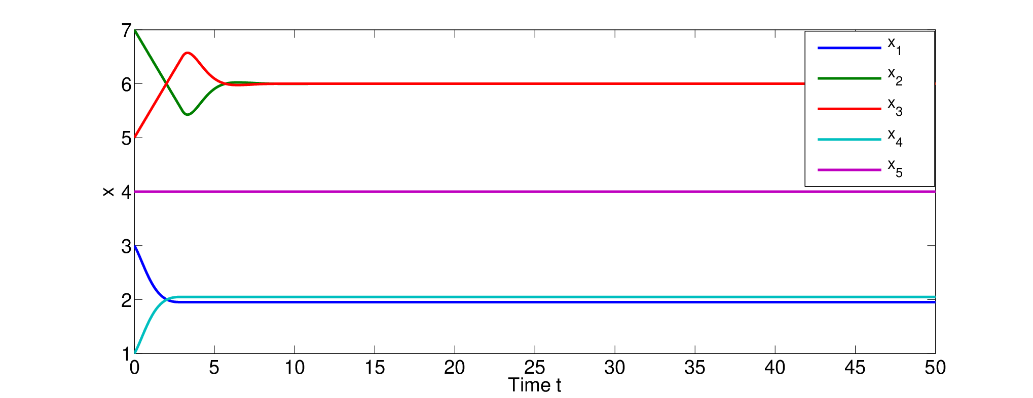
The same result can be deduced from the following analysis. In Figure 2, the smallest number of cycles to cover the whole graph is ; one option being , , . So where
| (51) |
In this case . By setting , the flow in reaches the upper bound, while the flows in reach the lower bounds, i.e.
| (52) |
Thus there exists an equilibrium satisfying .
6 Conclusions
We have discussed a basic model of dynamical distribution networks where the flows through the edges are generated by distributed PI controllers. The resulting system can be naturally modeled as a port-Hamiltonian system, enabling the easy derivation of sufficient and necessary conditions for the convergence of the state variables to load balancing (consensus). The main part of this paper focusses on the case where flow constraints are present. A key ingredient in this analysis is the construction of a Lyapunov function. We distinguish between the case that the flow constraints corresponding to all the edges allow for bi-directional flow and the case that all the edges only allow for uni-directional flow. For both cases we have derived necessary and sufficient conditions for asymptotic load balancing based on the structure of the graph.
An obvious open problem is the extension of our results to the general case where some of the edges allow bi-directional flow and others only uni-directional flow. This is currently under investigation. Many other questions can be addressed in this framework. For example, what is happening if the in/outflows are not assumed to be constant, but are e.g. periodic functions of time; see already [13]. Furthermore, the use of constrained PI-controllers may suggest a fruitful connection to anti-windup control ideas.
References
- [1] \bibinfoauthorA.J. van der Schaft and B.M. Maschke, \bibinfotitlePort-Hamiltonian systems on graphs, \bibinfojournalSIAM J. Control and Optimization (\bibinfoyear2013, to appear).
- [2] \bibinfoauthorA.J. van der Schaft and B.M. Maschke, \bibinfotitleConservation laws on higher-dimensional networks, \bibinfojournalProc. 47th IEEE Conf. on Decision and Control (\bibinfoyear2008) \bibinfopages799–804.
- [3] A.J. van der Schaft and B.M. Maschke, Model-Based Control: Bridging Rigorous Theory and Advanced Technology, P.M.J. Van den Hof, C. Scherer, P.S.C. Heuberger, eds., chapter Conservation laws and lumped system dynamics, Springer, Berlin-Heidelberg, 2009, pp.31–48.
- [4] \bibinfoauthorA.J. van der Schaft and B.M. Maschke, \bibinfotitlePort-Hamiltonian dynamics on graphs: Consensus and coordination control algorithms, \bibinfojournalProc. 2nd IFAC Workshop on Distributed Estimation and Control in Networked Systems,Annecy, France (\bibinfoyear2010) \bibinfopages175–178.
- [5] \bibinfoauthorM. Bürger and D. Zelazo and F. Allgöwer, \bibinfotitleNetwork clustering: A dynamical systems and saddle-point perspective, \bibinfojournalIEEE Conference on Decision and Control (\bibinfoyear2011) \bibinfopages7825–7830.
- [6] \bibinfoauthorD. Zelazo and M. Mesbahi, \bibinfotitleEdge agreement: Graph-theoretic performance bounds and passivity analysis, \bibinfojournalAutomatic Control, IEEE Transactions on \bibinfovolume56 (\bibinfoyear2011) \bibinfopages544 –555, doi:10.1109/TAC.2010.2056730.
- [7] \bibinfoauthorA.J. van der Schaft and J. Wei, \bibinfotitleA hamiltonian perspective on the control of dynamical distribution networks, \bibinfojournal4th IFAC Workshop on Lagrangian and Hamiltonian Methods for Non Linear Control (\bibinfoyear2012) \bibinfopages24–29.
- [8] \bibinfoauthorB. Bollobas, \bibinfotitleModern Graph Theory, volume \bibinfovolume184 of \bibinfoseriesGraduate Texts in Mathematics, \bibinfopublisherSpringer, \bibinfoaddressNew York, \bibinfoyear1998.
- [9] \bibinfoauthorA.J van der Schaft and B.M. Maschke, \bibinfotitleThe Hamiltonian formulation of energy conserving physical systems with external ports, \bibinfojournalArchiv für Elektronik und Übertragungstechnik \bibinfovolume49 (\bibinfoyear1995) \bibinfopages362–371.
- [10] A.J. van der Schaft, -Gain and Passivity Techniques in Nonlinear Control, Vol.218 of Lect. Notes in Control and Information Sciences, pringer-Verlag, Berlin, 1996, 2nd edition, Springer, London, 2000.
- [11] \bibinfoauthorB. Jayawardhana and R. Ortega and E. García-Canseco and F. Castaños, \bibinfotitlePassivity of nonlinear incremental systems: Application to PI stabilization of nonlinear RLC circuits, \bibinfojournalSystems & Control Letters \bibinfovolume56 (\bibinfoyear2007) \bibinfopages618–622.
- [12] \bibinfoauthorF. Blanchini and S. Miani and W. Ukovich, \bibinfotitleControl of production-distribution systems with unknown inputs and system failures., \bibinfojournalIEEE Transactions on Automatic Control \bibinfovolume45(6) (\bibinfoyear2000) \bibinfopages1072–1081.
- [13] \bibinfoauthorC. D. Persis, \bibinfotitleBalancing time-varying demand-supply in distribution networks: an internal model approach (\bibinfoyear2013).