Localized Dimension Growth: A Convolutional Random Network Coding Approach to Managing Memory and Decoding Delay

We model a communication network as a finite directed multigraph, denoted by $\mathcal{G}=(\mathcal{V},\mathcal{E})$, where $\mathcal{V}$ is the set of nodes and $\mathcal{E}$ is the set of edges. An edge represents a noiseless communication channel with unit capacity. We consider the single-source multicast case, i.e., the source sends the same messages to all the sinks in the network. The source node is denoted by $s$, and the set of $d$ sink nodes is denoted by $R=\{r_{1},\ldots,r_{d}\}\subset\mathcal{V}$. For every node $v\in\mathcal{V}$, the sets of incoming and outgoing channels to $v$ are $In(v)$ and $Out(v)$; let $In(s)$ be the empty set $\emptyset$. An ordered pair $(e^{\prime},e)$ of edges is called an adjacent pair when there exists a node $v$ with $e^{\prime}\in In(v)$ and $e\in Out(v)$. Since edges are directed, we use the terms edge and arc interchangeably in this paper.

The symbol alphabet is represented by a base field, $\mathbb{F}_{q}$. Assume $s$ generates a source message per unit time, consisting of a fixed number of $m$ source symbols represented by a size $m$ row vector $x_{t}=(x_{1,t},x_{2,t},\cdots,x_{m,t})$, $x_{i,t}\in\mathbb{F}_{q}$. Time $t$ is indexed from 0, with the $(t+1)$-th message is generated at time $t$. The source messages can be collectively represented by a power series $x(z)=\sum_{t\geq 0}{x_{t}z^{t}}$, where $x_{t}$ is the message generated at time $t$ and $z$ denotes a unit-time delay. $x(z)$ is therefore a row vector of polynomials from the ring $\mathbb{F}_{q}[z]$.

Collectively, we call the $|In(v)|\times|Out(v)|$ matrix $K_{v}(z)=(k_{e^{\prime},e}(z))_{e^{\prime}\in In(v),e\in Out(v)}=K_{v,0}+K_{v,1}z+K_{v,2}z^{2}+\ldots$ the local encoding kernel matrix at node $v$, and the $m\times|In(v)|$ matrix $F_{v}(z)=(f_{e}(z))_{e\in In(v)}$ the global encoding kernel matrix at node $v$. Observe from Eq. (2) that, at sink $r$, $F_{r}(z)$ is required to deconvolve the received data messages $y_{e^{\prime}_{i}}(z)$, $e^{\prime}_{i}\in In(r)$. Therefore, each intermediate node $v$ computes $f_{e}(z)$ for outgoing edges from $F_{v}(z)$ according to Eq.(3), and sends $f_{e}(z)$ along edge $e$, together with data $y_{e}(z)$. This can be achieved by arranging the coefficients of $f_{e}(z)$ in a vector form and attaching them to the data. In this paper, we ignore the effect of this overhead transmission of coding coefficients on throughput or delay: we show in Section III-B that the number of terms in $f_{e}(z)$ is finite, thus the overhead can be amortized over a long period of data transmissions.

Moreover, $F_{v}(z)$ can be written as $F_{v}(z)=F_{v,0}+F_{v,1}z+\cdots+F_{v,t}z^{t}$, where $F_{v,t}\in\mathbb{F}_{q}^{m\times In(v)}$ is the global encoding kernel matrix at time $t$. $F_{v}(z)$ can thus be viewed as a polynomial, with $F_{v,t}$ as matrix coefficients. Let $L_{v}$ be the degree of $F_{v}(z)$. $L_{v}+1$ is a direct measure of the amount of memory required to store $F_{v}(z)$. We shall define in Section III-C the metric used to measure memory overhead of ARCNC.

In an acyclic network, the local and global encoding kernel descriptions of a linear network code are equivalent, in the sense that for a given set of local encoding kernels, a set of global encoding kernels can be calculated recursively in any upstream-to-downstream order. In other words, a code generated from local encoding kernels has a unique solution when decoding is performed on the corresponding global encoding kernels. By comparison, in a cyclic network, partial orderings of edges or nodes are not always consistent. Given a set of local encoding kernels, there may exist a unique, none, or multiple sets of global encoding kernels (§3.1, [15]). If the code is non-unique, the decoding process at a sink may fail. A sufficient condition for a CNC to be successful is that the constant coefficient matrix consisting of all local encoding kernels be nilpotent [16]; this condition is satisfied if we code over an acyclic topology at $t=0$ [12]. In the extreme case, all local encoding kernels can be set to 0 at $t=0$. This setup translates to a unit transmission delay on each link, which as previous work on RLNC has shown, guarantees the uniqueness of a code construction [3]. To minimize decoding delay, it is intuitive to make as few local encoding kernels zero as possible. In other words, a reasonable heuristic is to assign 0 to a minimum number of $k_{e^{\prime},e,0}$, $(e^{\prime},e)\in\mathcal{E}$, and to assign values chosen uniformly randomly from $\mathbb{F}_{q}$ to the rest. The goal is to guarantee that each cycle contains at least a single delay.

Although seemingly similar, this process is actually not the same as the problem of finding the minimal feedback edge set. A feedback edge set is a set containing at least one edge of every cycle in the graph. When a feedback edge set is removed, the graph becomes an acyclic directed graph. In our setup, however, since $k_{e^{\prime},e,0}$ is specific to an adjacent edge pair, $k_{e^{\prime},e,0}$ does not need to be 0 for all $e^{\prime}$ where $(e^{\prime},e)\in\mathcal{V}$.

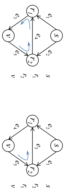
For example, a very simple but not necessarily delay-optimal heuristic is to index all edges, and to assign 0 to $k_{e^{\prime},e,0}$ if $e^{\prime}\succeq e$, i.e., when $e^{\prime}$ has an index larger than $e$; $k_{e^{\prime},e,0}$ is chosen randomly from $\mathbb{F}_{q}$ if $e^{\prime}\prec e$. Fig. 1 illustrates this indexing scheme. A node is considered to be visited if one of its incoming edges has been indexed; a node is put into a queue once it is visited. For each node removed from the queue, numerical indices are assigned to all of its outgoing edges. Nodes are traversed starting from the source $s$. The outgoing edges of $s$ are therefore numbered from 1 to $|Out(s)|$. Note that the index set thus obtained is not necessarily unique. In this particular example, we can have two sets of edge indices, as shown in Fig. 1. Here $r_{1}$ is visited before $r_{2}$ on the left, and vice versa on the right. In each case, an adjacent pair $(e^{\prime},e)$ is highlighted with a curved arrow if $e^{\prime}\succeq e$. At $t=0$, we set $k_{e^{\prime},e,0}$ to 0 for such highlighted adjacent pairs, and choose $k_{e^{\prime},e,0}$ uniformly randomly from $\mathbb{F}_{q}$ for other adjacent pairs.

Observe that, in an acyclic network, this indexing scheme provides a total ordering for the nodes as well as for the edges: a node is visited only after all of its parents and ancestors are visited; an edge is indexed only after all edges on any of its paths from the source are indexed. In a cyclic network, however, an order of nodes and edges is only partial, with inconsistencies around each cycle. Such contradictions in the partial ordering of edges make the generation of unique network codes along each cycle impossible. By assigning 0 to local encoding kernels $k_{e^{\prime},e,0}$ for which $e^{\prime}\succeq e$, such inconsistencies can be avoided at time 0, since the order of $e^{\prime}$ and $e$ becomes irrelevant in determining the network code. After the initial step, $k_{e^{\prime},e,t}$ is not necessarily 0 for $e^{\prime}\succeq e$, $t>0$, nonetheless the convolution operations at intermediate nodes ensure that the 0 coefficient inserted at $t=0$ makes the global encoding kernels unique at the sinks. This idea can be derived from the expression for $f_{e,t}$ given in Eq. (4). In each cycle, there is at least one $k_{e^{\prime},e,0}$ that is equal to zero. The corresponding $f_{e^{\prime},t}$ therefore does not contribute to the construction of other $f_{e,t}$’s in the cycle. In other words, the partial ordering of arcs in the cycle can be considered consistent at $t=1$ and later times.

Although this heuristic for cyclic networks is not optimal, it is universal. One disadvantage of this approach is that full knowledge of the topology is required at $t=0$, making the algorithm centralized instead of entirely distributed. Nonetheless, if inserting an additional transmission delay on each link is not an issue, we can always bypass this code assignment stage by zeroing all local encoding kernels at $t=0$.

After initialization, the algorithm proceeds in exactly the same way as in the acyclic case.

Discussions in [3, 2, 16] state that in a network with delays, ANC gives rise to random processes which can be written algebraically in terms of a delay variable $z$. Thus, a convolutional code can naturally evolve from message propagation and linear encoding. ANC in the delay-free case is therefore equivalent to CNC with constraint length 1. Similarly, using a CNC with constraint length $l>1$ on a delay-free network is equivalent to performing ANC on the same network, but with $l-1$ self-loops attached to each encoding node. Each self-loop carries $z,z^{2},\ldots,z^{l-1}$ units of delay respectively.

For example, in Fig. 2, we show a node with two incoming edges. Let the data symbol transmitted on edge $\dot{e}$ at time $t$ be $y_{\dot{e},t}$. A CNC with length $l=2$ is used in (a), assuming that transmissions are delay-free. The local encoding kernel matrix $K_{\text{CNC}}(z)$ contains two polynomials, $k_{e^{\prime},e_{1}}(z)=k_{e^{\prime},e_{1},0}+k_{e^{\prime},e_{1},1}z$ and $k_{e^{\prime\prime},e_{1}}(z)=k_{e^{\prime\prime},e_{1},0}+k_{e^{\prime\prime},e_{1},1}z$. According to Eq. (1) and (5), the data symbol transmitted on $e_{1}$ at time $t$ is

In (b), the equivalent ANC is shown. A single loop with a transmission delay of $z$ has been added, and the local encoding kernel matrix $K_{\text{ANC}}=(k_{\dot{e},e})_{\dot{e}\in In(v),e\in Out(v)}$ is constructed from coding coefficients from (a). The first column of $K_{\text{ANC}}$ represents encoding coefficients from incoming edges $e^{\prime},e^{\prime\prime},e^{\prime\prime\prime}$ to the outgoing edge $e_{2}$, and the second column represents encoding coefficients from incoming edges $e^{\prime},e^{\prime\prime},e^{\prime\prime\prime}$ to the outgoing edge $e^{\prime\prime\prime}$. Using a matrix notation, the output data symbols from $v$ are $(y_{e_{2},t}\quad y_{e^{\prime\prime\prime},t})=(y_{e^{\prime},t}\quad y_{e^{\prime\prime},t}\quad y_{e^{\prime\prime\prime},t-1})K_{\text{ANC}}$, i.e.,

Clearly $y_{e_{1},t}$ is equal to $y_{e_{2},t}$. ARCNC therefore falls into the framework given by Ho et al. [3], in the sense that the convolution process either arises naturally from cycles with delays, or can be considered as computed over self-loops appended to acyclic networks. Applying the analysis from [3], we have the following theorem,

As discussed in Section II-B2, we define the first decoding time $T_{r}$ for sink $r$, $1\leq r\leq d$, as the time it takes $r$ to achieve decodability for the first time. We had called this variable the stopping time in [9]. Also recall that when all sinks are able to decode, at each sink $r$, $T_{r}$ can be smaller than $L_{r}$, the degree of the global encoding kernel matrix $F_{r}(z)$. Denote by $T_{N}$ the time it takes for all sinks in the network to successfully decode, i.e., $T_{N}=\max\{T_{1},\ldots,T_{d}\}$, then $T_{N}$ is also equal to $\max\{L_{1},\ldots,L_{d}\}$. The following corollary holds:

To measure the amount of memory required by ARCNC, first recall from Section II-A that at each node $v$, the global encoding kernel matrix $F_{v}(z)$, the local encoding kernel matrix $K_{v}(z)$, and past data $y_{e^{\prime}}(z)$ on incoming arcs $e^{\prime}\in In(v)$ need to be stored in memory. $K_{v}(z)$ and $y_{e^{\prime}}(z)$ should always be saved because together they generate new data symbols to transmit (see Eqs. (1) and (5)). $F_{v}(z)$ should be saved during the code construction process at intermediate nodes, and always at sinks, since they are needed for decoding.

Let us consider individually the three contributors to memory use. Firstly, recall from Section II-A that $F_{v}(z)$ can be viewed as a polynomial in $z$. When all sinks are able to decode, at node $v$, $F_{v}(z)$ has degree $L_{v}$, with coefficients from $\mathbb{F}_{q}^{m\times In(v)}$. The total amount of memory needed for $F_{v}(z)$ is therefore proportional to $\lceil\log_{2}q\rceil mIn(v)(L_{v}+1)$. Secondly, from Eq. (4), we see that the length of a local encoding kernel polynomial $k_{e^{\prime},e}(z)$ should be equal to or smaller than that of $f_{e}(z)$. Thus, the length of $K_{v}(z)$ should also be equal to or smaller than that of $F_{v}(z)$. The coefficients of $K_{v}(z)$ are elements of $\mathbb{F}_{q}^{In(v)\times Out(v)}$. Hence, the amount of memory needed for $K_{v}(z)$ is proportional to $\lceil\log_{2}q\rceil Out(v)In(v)(L_{v}+1)$. Lastly, a direct comparison between Eqs. (4) and (5) shows that memory needed for $y_{e^{\prime}}(z)$, $e^{\prime}\in In(v)$ is the same for that needed for $F_{v}(z)$. In practical uses of network coding, data can be transmitted in packets, where symbols are concatenated and operated upon in parallel. Packets can be very long in length. Nonetheless, the exact packet size is irrelevant for comparing memory use between different network codes, since all comparisons are naturally normalized to packet lengths.

One point to keep in mind when measuring memory use is that even after a sink achieves decodability, its code length can still increase, as long as at least one of its ancestors has not stopped increasing code length. We say a non-source node $v$ is related to a sink $r$ if $v$ is an ancestor of $r$, or if $v$ shares an ancestor, other than the source, with $r$. Hence, $L_{r}$ is dependent on all nodes related to $r$.

To study the computation complexity of ARCNC, first observe that, once the adaptation process terminates, the computation needed for the ensuing code is no more than a regular CNC. In fact, the expected computation complexity is proportional to the average code length of ARCNC. We therefore omit the details of the complexity analysis of regular CNC here and refer interested readers to [7].

For the adaptation process, the encoding operations are described by Eq. (4). If the algorithm stops at time $T_{N}$, the number of operations in the encoding steps is $O(D_{in}|\mathcal{E}|T_{N}^{2}m)$, where $D_{in}=\max_{v\in\mathcal{V}}|In(v)|$.

To determine decodability at a sink $r$, we check if the rank of $F_{r}(z)$ is $m$. A straight-forward approach is to check whether its determinant is a non-zero polynomial. Alternatively, Gaussian elimination could be applied. At time $t$, because $F_{r}(z)$ is an $m\times|In(r)|$ matrix and each entry is a polynomial with degree $t$, the complexity of checking whether $F_{r}(z)$ is full rank is $O(D_{in}^{2}2^{m}mt^{2})$. Instead of computing the determinant or using Gaussian elimination directly, we propose to check the conditions given in Section II-B. For each sink $r$, at time $t$, determining $rank\left({\begin{array}[]{*{20}c}F_{0}&F_{1}&\cdots F_{t}\end{array}}\right)$ requires $O(D_{in}^{2}mt^{2})$ operations. If the first test passes, we calculate $rank(M_{t})$ and $rank(M_{t-1})$ next. Observe that $rank(M_{t-1})$ was computed during the last iteration. $M_{t}$ is a $(t+1)m\times(t+1)|In(r)|$ matrix over field $\mathbb{F}_{q}$. The complexity of calculating $rank(M_{t})$ by Gaussian elimination is $O(D_{in}^{2}mt^{3})$. The process of checking decodability is performed during the adaptation process only, hence the computation complexity here can be amortized over time after the coding coefficients are determined. In addition, as decoding occurs symbol-by-symbol, the adaptation process itself does not impose any additional delays.

A $n\choose m$ combination network contains a single source $s$ that multicasts $m$ independent messages over $\mathbb{F}_{q}$ through $n$ intermediate nodes to $d$ sinks [15]; each sink is connected to a distinct set of $m$ intermediate nodes, and $d={n\choose m}$. Fig. 3 illustrates the topology of a combination network. Assuming unit capacity links, the min-cut to each sink is $m$. It can be shown that, in combination networks, routing is insufficient and network coding is needed to achieve the multicast capacity $m$. Here coding is performed only at $s$, since each intermediate node has only $s$ as a parent node; an intermediate node simply relays to its children data from $s$. For a general $n\choose m$ combination network, we showed in [9] that the expected average first decoding time can be significantly improved by ARCNC when compared to the deterministic BNC algorithm. We restate the results here, with details of the derivations included.

At time $t-1$, for a sink $r$ that has not satisfied the decodability conditions, $F_{r}(z)$ is a size $m\times m$ matrix of polynomials of degree $t-1$. $F_{r}(z)$ has full rank with probability

Hence, the probability that sink $r$ decodes after time $t-1$ is

The expected first decoding time for sink node $r$ is therefore upper and lower-bounded as follows.

Recall from Section III-B that the expected average first decoding time is $E[T_{\text{avg}}]=E\left[\frac{1}{d}\sum_{r=1}^{d}T_{r}\right]$. In a combination network, $E[T_{\text{avg}}]$ is equal to $E[T_{r}]$. Consequently, $E[T_{\text{avg}}]$ is upper-bounded by $ET_{UB}$, defined by Eq. (19). $ET_{UB}$ is a function of $m$ and $q$ only, independent of $n$. For example, if $m=2$, $q=2$, $ET_{UB}=\frac{5}{3}$. If $m$ is fixed, but $n$ increases, $E[T_{\text{avg}}]$ does not change. In addition, if $q$ is large, $ET_{UB}$ becomes 0, consistent with the general analysis in [9].

Next, we want to bound the variance of $T_{\text{avg}}$, i.e.,

We upper-bound the terms above one by one. First,

References

- [1] R. Ahlswede, N. Cai, S. Li, and R. Yeung, “Network information flow,” IEEE Trans. on Info. Theory, vol. 46, no. 4, pp. 1204–1216, 2000.
- [2] R. Li, S.Y.R.Yeung and N. Cai, “Linear network coding,” IEEE Trans. on Info. Theory, vol. 49, no. 2, pp. 371–381, 2003.
- [3] T. Ho, M. Médard, R. Koetter, D. Karger, M. Effros, J. Shi, and B. Leong, “A random linear network coding approach to multicast,” IEEE Trans. on Info. Theory, vol. 52, no. 10, pp. 4413–4430, 2006.
- [4] M. Médard, M. Effros, D. Karger, and T. Ho, “On coding for non-multicast networks,” in Proc. of the 41st Allerton Conference, vol. 41, no. 1, 2003, pp. 21–29.
- [5] S. Jaggi, P. Sanders, P. Chou, M. Effros, S. Egner, K. Jain, and L. Tolhuizen, “Polynomial time algorithms for multicast network code construction,” IEEE Trans. on Info. Theory, vol. 51, no. 6, pp. 1973–1982, 2005.
- [6] S. Li and R. Yeung, “On convolutional network coding,” in Proc. of IEEE Int. Sym. on Info. Theory, 2006, pp. 1743–1747.
- [7] E. Erez and M. Feder, “Convolutional network codes,” in Proc. of IEEE Int. Sym. on Info. Theory (ISIT), 2005, p. 146.
- [8] M. Xiao, M. Médard, and T. Aulin, “A binary coding approach for combination networks and general erasure networks,” in Proc. of IEEE Int. Sym. on Info. Theory (ISIT), 2008, pp. 786–790.
- [9] W. Guo, N. Cai, X. Shi, and M. Medard, “Localized dimension growth in random network coding: A convolutional approach,” in Proc. of IEEE Int. Sym. on Info. Theory (ISIT), 2011, pp. 1156–1160.
- [10] T. Ho, S. Jaggi, S. Vyetrenko, and L. Xia, “Universal and robust distributed network codes,” in 2011 IEEE Proceedings of INFOCOM, 2010, pp. 766–774.
- [11] C. Ngai and R. Yeung, “Network coding gain of combination networks,” in Proc. of IEEE Info. Theory Workshop, 2004, pp. 283–287.
- [12] N. Cai and W. Guo, “The conditions to determine convolutional network coding on matrix representation,” in Proc. NetCod, 2009, pp. 24–29.
- [13] J. Massey and M. Sain, “Inverses of linear sequential circuits,” IEEE Trans. on Comp., vol. 100, no. 4, pp. 330–337, 2006.
- [14] W. G. Guo, N. Cai, and Q. T. Sun, “Time-Variant Decoding of Convolutional Network Codes,” IEEE Communications Letters, vol. 16, no. 10, pp. 1656–1659, 2012.
- [15] R. Yeung, S. Li, N. Cai, and Z. Zhang, “Network Coding Theory: Single Sources,” Foundations and Trends® in Communications and Information Theory, vol. 2, no. 4, pp. 241–329, 2005.
- [16] R. Koetter and M. Médard, “An algebraic approach to network coding,” IEEE/ACM Trans. on Networking, vol. 11, no. 5, pp. 782–795, 2003.
- [17] H. Balli, X. Yan, and Z. Zhang, “On randomized linear network codes and their error correction capabilities,” IEEE Trans. on Info. Theory, vol. 55, no. 7, pp. 3148–3160, 2009.
- [18] M. Newman, “Random graphs as models of networks,” Handbook of Graphs and Networks, pp. 35–68, 2003.