Subgraphs Satisfying MSO Properties on -Topologically Orderable Digraphs
Abstract
We introduce the notion of -topological orderings for digraphs. We prove that given a digraph on vertices admitting a -topological ordering, together with such an ordering, one may count the number of subgraphs of that at the same time satisfy a monadic second order formula and are the union of directed paths, in time . Our result implies the polynomial time solvability of many natural counting problems on digraphs admitting -topological orderings for constant values of and . Concerning the relationship between -topological orderability and other digraph width measures, we observe that any digraph of directed path-width has a -topological ordering for . On the other hand, there are digraphs on vertices admitting a -topological order for , but whose directed path-width is . Since graphs of bounded directed path-width can have both arbitrarily large undirected tree-width and arbitrarily large clique width, our result provides for the first time a suitable way of partially transposing metatheorems developed in the context of the monadic second order logic of graphs of constant undirected tree-width and constant clique width to the realm of digraph width measures that are closed under taking subgraphs and whose constant levels incorporate families of graphs of arbitrarily large undirected tree-width and arbitrarily large clique width.
Keywords:
Slice Theory, Digraph Width Measures, Monadic Second Order Logic of Graphs, Algorithmic Meta-theorems1 Introduction
Two cornerstones of parametrized complexity theory are Courcelle’s theorem [13] stating that monadic second order logic properties may be model checked in linear time in graphs of constant undirected tree-width, and its subsequent generalization to counting given by Arnborg, Lagergren and Seese [2]. The importance of such metatheorems stem from the fact that several NP-complete problems such as Hamiltonicity, colorability, and their respective P-hard counting counterparts, can be modeled in terms of sentences and thus can be efficiently solved in graphs of constant undirected tree-width.
In this work we introduce the notion of -topological orderings for digraphs and provide a suitable way of partially transposing the metatheorems in [13, 2] to digraphs admitting -topological orderings for constant values of . In order to state our main result we will first give a couple of easy definitions: Let be a directed graph. For subsets of vertices we let denote the set of edges with one endpoint in and another endpoint in . We say that a linear ordering of the vertices of is a -topological ordering of if for every directed simple path in and every with , we have that . In other words, is a -topological ordering if every directed simple path of bounces back and forth at most times along . The terminology -topological ordering is justified by the fact that any topological ordering of a DAG according to the usual definition, is a -topological ordering according to our definition. Conversely if a digraph admits a -topological ordering, then it is a DAG. We denote by the monadic second order logic of graphs with edge set quantification. An edge-weighting function for a digraph is a function where is a finite commutative semigroup of size polynomial in whose elements are totally ordered. The weight of a subgraph of is defined as . A maximal-weight subgraph of satisfying a given property is a subgraph such that and such that for any other subgraph of such that we have . Now we are in a position to state our main theorem:
Theorem 1.1 (Main Theorem)
For each formula and each positive integers there exists a computable function such that: Given a digraph of zig-zag number on vertices, a weighting function , a -topological ordering of and a number 11 1 Observe that can be as large as ., we can count in time the number of subgraphs of simultaneously satisfying the following four properties:
- (i)
- (ii)
is the union of directed paths22 2 A digraph is the union of directed paths if for not necessarily vertex-disjoint nor edge-disjoint directed paths .
- (iii)
has vertices
- (iv)
has maximal weight
Our result implies the polynomial time solvability of many natural counting problems on digraphs admitting -topological orderings for constant values of and . We observe that graphs admitting -topological orderings for constant values of can already have simultaneously unbounded tree-width and unbounded clique-width, and therefore the problems that we deal with here cannot be tackled by the approaches in [13, 2, 15]. For instance any DAG is -topologically orderable. In particular, the directed grid in which all horizontal edges are directed to the left and all vertical edges oriented up is -topologically orderable, while it has both undirected tree-width and clique-width .
2 Applications
To illustrate the applicability of Theorem 1.1 with a simple example, suppose we wish to count the number of Hamiltonian cycles on . Then our formula will express that the graphs we are aiming to count are cycles, namely, connected graphs in which each vertex has degree precisely two. Such a formula can be easily specified in . Since any cycle is the union of two directed paths, we have . Since we want all vertices to be visited our . Finally, the weights in this case are not relevant, so it is enough to set the semigroup to be the one element semigroup , and the weights of all edges to be . In particular the total weight of any subgraph of according to this semigroup will be . By Theorem 1.1 we can count the number of Hamiltonian cycles in in time . We observe that Hamiltonicity can be solved within the same time bounds for other directed width measures, such as directed tree-width [33].
Interestingly, Theorem 1.1 allow us to count structures that are much more complex than cycles. And in our opinion it is rather surprising that counting such complex structures can be done in XP. For instance, we could choose to count the number of maximal Hamiltonian subgraphs of which can be written as the union of directed paths. We can repeat this trick with virtually any natural property that is expressible in . For instance we can count the number of maximal weight -colorable subgraphs of that are the union of -paths. Or the number of subgraphs of that are the union of directed paths and have di-cuts of size . Observe that our framework does not allow one to find a maximal di-cut of the whole graph nor to determine in polynomial time whether the whole graph is 3-colorable, since these problems are already NP-complete for DAGs, i.e., for .
If is a digraph, then the disorientation of is the undirected graph obtained from by forgetting the orientation of its edges. In other words, we add an edge to whenever . A very interesting application of Theorem 1.1 consists in counting the number of maximal-weight subgraphs of which are the union of paths and whose disorientation satisfy some structural property, such as, connectedness, planarity, bounded genus, bipartiteness, etc. The proof of the next corollary can be found in Appendix 0.B.
Corollary 1
Let be a digraph on vertices and be an edge weighting function. Then given a -topological ordering of one may count in time the number of maximal-weight subgraphs that are the union of directed paths and satisfy any combination of the following properties: Connectedness, Being a forest, Bipartiteness, Planarity, Constant Genus , Outerplanarity, Being Series Parallel, Having Constant Treewidth ) Having Constant Branchwidth , ) Satisfy any minor closed property.
The families of problems described above already incorporate a large number of natural combinatorial problems. However the monadic second order formulas expressing the problems above are relatively simple and can be written with at most two quantifier alternations. As Matz and Thomas have shown however, the monadic second order alternation hierarchy is infinite [38]. Additionally Ajtai, Fagin and Stockmeyer showed that each level of the polynomial hierarchy has a very natural complete problem, the -round--coloring problem, that belongs to the -th level of the monadic second order hierarchy (Theorem 11.4 of [1]). Thus by Theorem 1.1 we may count the number of -round-3-colorable subgraphs of that are the union of directed paths in time .
We observe that the condition that the subgraphs we consider are the union of directed paths is not as restrictive as it might appear at a first glance. For instance one can show that for any the undirected grid is the union of directed paths. Additionally these grids have zig-zag number number . Therefore counting the number of maximal grids of height on a digraph of zig-zag number is a neat example of problem which can be tackled by our techniques but which cannot be formulated as a linkage problem, namely, the most successful class of problems that has been shown to be solvable in polynomial time for constant values of several digraph width measures [33].
3 Overview of the Proof of Theorem 1.1
We will prove Theorem 1.1 within the framework of regular slice languages, which was originally developed by the author to tackle several problems within the partial order theory of concurrency [17, 18]. The main steps of the proof of Theorem 1.1 are as follows. To each regular slice language we associate a possibly infinite set of digraphs . In Section 7 we will define the notion of -dilated-saturated regular slice language and show that given any digraph together with a -topological ordering of , and any -dilated-saturated slice language , one may efficiently count the number of subgraphs of that are isomorphic to some digraph in ( Theorem 7.2). Then in Section 8 we will show that given any monadic second order formula and any natural numbers one can construct a -dilated-saturated regular slice language representing the set of all digraphs that at the same time satisfy and are the union of directed paths (Theorem 8.1). The construction of is done once and for all for each , and , and is completely independent from the digraph . Finally, the proof of Theorem 1.1 will follow by plugging Theorem 8.1 into Theorem 7.2. Proofs of intermediate results omitted for a matter of clarity or due to lack of space can be found in the appendix.
4 Comparison With Existing Work
Since the last decade, the possibility of lifting the metatheorems in [13, 2] to the directed setting has been an active line of research. Indeed, following an approach delineated by Reeds [41] and Johnson, Robertson, Seymour and Thomas [33], several digraph width measures have been defined in terms of the number of cops needed to capture a robber in a certain evasion game on digraphs. From these variations we can cite for example, directed tree-width [41, 33], DAG width [6], D-width [42, 29], directed path-width [4], entanglement [7, 8], Kelly width [32] and Cycle Rank [20, 31]. All these width measures have in common the fact that DAGs have the lowest possible constant width ( or depending on the measure). Other width measures in which DAGs do not have necessarily constant width include DAG-depth [24], and Kenny-width [24].
The introduction of the digraph width measures listed above was often accompanied by algorithmic implications. For instance, certain linkage problems that are NP-complete for general graphs, e.g. Hamiltonicity, can be solved efficiently in graphs of constant directed tree-width [33]. The winner of certain parity games of relevance to the theory of -calculus can be determined efficiently in digraphs of constant DAG width [6], while it is not known if the same can be done for general digraphs. Computing disjoint paths of minimal weight, a problem which is NP-complete in general digraphs, can be solved efficiently in graphs of bounded Kelly width. However, except for such sporadic successful algorithmic implications, researchers have failed to come up with an analog of Courcelle’s theorem for graph classes of constant width for any of the digraph width measures described above. It turns out that there is a natural barrier against this goal: It can be shown that unless all the problems in the polynomial hierarchy have sub-exponential algorithms, which is a highly unlikely assumption, model checking is intractable in any class of graphs that is closed under taking subgraphs and whose undirected tree-width is poly-logarithmic unbounded [34, 35]. An analogous result can be proved with respect to model checking of properties if we assume a non-uniform version of the extended exponential time hypothesis [26, 25]. All classes of digraphs of constant width with respect to the directed measures described above are closed under subgraphs and have poly-logarithmically unbounded tree-width, and thus fall into the impossibility theorem of [34, 35]. It is worth noting that Courcelle, Makowsky and Rotics have shown that model checking is tractable in classes of graphs of constant clique-width [15, 16], and that these classes are poly-logarithmic unbounded, but they are not closed under taking subgraphs.
We define the zig-zag number of a digraph to be the minimum for which has a -topological ordering, and denote it by . The zig-zag number is a digraph width measure that is closed under taking subgraphs and that has interesting connections with some of the width measures described above. In particular we can prove the following theorem stating that families of graphs of constant zig-zag number are strictly richer than families of graphs of constant directed path-width.
Theorem 4.1
Let be a digraph of directed path-width . Then has zig-zag number . Furthermore, given a directed path decomposition of one can efficiently derive a -topological ordering of . On the other hand, there are digraphs on vertices whose zig-zag number is but whose directed path-width is .
Theorem 4.1 legitimizes the algorithmic relevance of Theorem 1.1 since path-decompositions of graphs of constant directed path-width can be computed in polynomial time [44]. The same holds with respect to the cycle rank of a graph since constant cycle-rank decompositions33 3 By cycle-rank decomposition we mean a direct elimination forest[30]. can be converted into constant directed-path decompositions in polynomial time [30]. Therefore all the problems described in Section 1 can be solved efficiently in graphs of constant directed path-width and in graphs of constant cycle rank. We should notice that our main theorem circumvents the impossibility results of [34, 35, 26, 25] by confining the monadic second order logic properties to subgraphs that are the union of directed paths.
A pertinent question consists in determining whether we can eliminate either or from the exponent of the running time stated in Theorem 1.1. The following two theorems say that under strongly plausible parameterized complexity assumptions [19], namely that and , the dependence of both and in the exponent of the running time is unavoidable.
Theorem 4.2 (Lampis-Kaouri-Mitsou[36])
Determining whether a digraph of cycle rank has a Hamiltonian circuit is hard with respect to .
Since by Theorem 4.1 constant cycle rank is less expressive than constant zig-zag number, the hardness result stated in Theorem 4.2 also works for zig-zag number. Given a sequence of not necessarily distinct vertices , a -linkage is a set of internally disjoint directed paths where each connects to .
Theorem 4.3 (Slivikins[43])
Given a , determining whether has a -linkage is hard for .
Thus, since a -linkage is clearly the union of -paths, Theorem 4.3 implies that the dependence of on the exponent is necessary even if is fixed to be .
5 Zig-Zag Number versus Other Digraph Width Measures
Cops-and-robber games provide an intuitive way to define several of the directed width measures cited in Section 4. Let be a digraph. A cops-and-robber game on is played by two parties. One is controlling a set of cops and the other is controlling a robber. At each round of the game the cop either stands on a vertex of or flies in an helicopter, meaning that it is temporarily removed from the digraph. The robber stands on a vertex of , and can at any time run at great speed along a cop-free directed path to another vertex. The objective of the cops is to capture the robber by landing on a vertex currently occupied by him, while the objective of the robber is to avoid capture.
Let be the minimum number of cops needed to capture the robber in a digraph . The directed tree-width of () is equal to if at each round the robber only moves to a vertex within the strongly connected component (SCC) induced by the vertices that are not blocked by cops [33]. The -width of () is equal to if the cops capture the robber according to a monotone strategy, i.e., cops never revisit vertices that were previously occupied by some cop. The robber is also required to move within the SCC induced by the non-blocked vertices[30]. The DAG-width of () is equal to when the cops follow a monotone strategy but when the robber can move along arbitrary cop free paths, independently of whether it stays within the SCC component induced by the non-blocked vertices [6]. The directed path width of () is equal to the quantity if we add the additional complication that the cops cannot see the robber [4]. The Kelly-width of () is equal to if the cops cannot see the robber and if at each step the robber only moves when a cop is about to land in his current position[24]. Finally, the DAG-depth of (), which is the directed analog of the tree-depth defined in [39], is the minimum number of cops needed to capture the robber when the cops follow a lift-free strategy, i.e., the cop player never moves a cop from a vertex once it has landed [24].
Some other width measures are better defined via some structural property. For instance, the K-width of () is the maximum number of different simple paths between any two vertices of [24]. The weak separator number of is defined as follows: If is a digraph and , then a weak balanced separator for is a set such that every SCC of contains at most vertices. The weak separator number of , denoted by is defined as the maximum size taken over all subsets , among the minimum weak balanced separators of . Finally, the cycle rank of a digraph denoted by is inductively defined as follows: If is acyclic, then . If is strongly connected and , then . If is not strongly connected then equals the maximum cycle rank among all strongly connected components of . Below we find a summary of the relations between the zig-zag number of a digraph and all the digraph width measures listed above. We write to indicate that there are graphs of constant width with respect to the measure but unbounded width with respect to the measure . We write to express that is not asymptotically greater than .
| (1) |
| (2) |
| (3) |
The numbers above and point to the references in which these relations where established. The only new relations are , and for which we provide a justification in the appendix.
6 Regular Slice Languages
A slice is a digraph comprising a set of vertices , a set of edges , a vertex labeling function for some set of symbols , and functions which respectively associate to each edge , a source vertex and a tail vertex . We notice that an edge might possibly have the same source and tail (). The vertex set is partitioned into three disjoint subsets: an in-frontier a center and an out-frontier . Additionally, we require that each frontier-vertex in is the endpoint of exactly one edge in and that no edge in has both endpoints in the same frontier. The function is an orienting function with the restriction that if , and if . Intuitively assigns to an edge if it is oriented towards the out frontier and if it is oriented towards the in-frontier. The frontier vertices in are labeled by with numbers from the set for some natural number in such a way that no two vertices in the same frontier receive the same number. Vertices belonging to different frontiers may on the other hand be labeled with the same number. The center vertices in are labeled by with elements from . We say that a slice is normalized if and . Non-normalized slices will play an important role in Section 7. Since we will deal with weighted graphs, we will also allow the edges of a slice to be weighted by a function where is a finite commutative semigroup.
A slice with frontiers can be glued to a slice with frontiers provided and provided that whenever and . In that case the glueing gives rise to the slice with frontiers which is obtained by fusing each such a pair of edges into a single edge whose orientation is coherent with the orientation of and 44 4 By coherent we mean and if and and if . (Figure 1.). We observe that in the glueing process the frontier vertices disappear. If and are weighted by functions and , then we add the requirement that the glueing of with can be performed if the weights of the edges touching the out-frontier of agree with the weights of their corresponding edges touching the in-frontier of . On the other hand, any slice can be decomposed into a sequence of atomic parts which we call unit slices, namely, slices with at most one vertex on its center (Figure 1.). Thus slices may be regarded as a graph theoretic analog of the knot theoretic braids [3], in which twists are replaced by vertices. Within automata theory, slices may be related to a vast number of formalisms such as graph automata [45, 11], graph rewriting systems [12, 5, 21], and others [28, 27, 10, 9]. In particular, slices may be regarded as a specialized version of the multi-pointed graphs defined in [21] but subject to a slightly different composition operation.
The width of a slice with frontiers is defined as . In the same way that letters from an alphabet may be concatenated by automata to form infinite languages of strings, we may use automata or regular expressions over alphabets of slices of a bounded width to define infinite families of digraphs. Let denote the set of all unit slices of width at most and whose frontier vertices are numbered with numbers from for . We say that a slice is initial if its in-frontier is empty and final if its out-frontier is empty. A slice with empty center is called a permutation slice. Due to the restriction that each frontier vertex of a slice must be connected to precisely one edge, we have that each vertex in the in-frontier of a permutation slice is necessarily connected to a unique vertex in its out-frontier. The empty slice, denoted by , is the slice with empty center and empty frontiers. We regard the empty slice as a permutation slice. A subset of the free monoid generated by is a slice language if for every sequence of slices we have that is an initial slice, a final slice and can be glued to for each . We should notice that at this point the operation of the monoid in consideration is just the concatenation of slice symbols and and should not be confused with the composition of slices. Also the unit of the monoid is just the empty symbol and not the empty slice, thus the elements of are simply sequences of slices, regarded as dumb letters. To each slice language over we associate a graph language consisting of all digraphs that are obtained by composing the elements of the strings in :
| (4) |
However we observe that a set of digraphs may be represented by several different slice languages, since a digraph in may be decomposed in several ways as a string of unit slices. We will use the term unit decomposition of a digraph to denote any sequence of unit slices whose composition yields . We say that the unit decomposition is dilated if it contains permutation slices, including possibly the empty slice (Figure 2.). The slice-width of is the minimal for which for some . In other words, the slice width of a unit decomposition is the width of the widest slice appearing in it.
A slice language is regular if it is generated by a finite automaton or regular expressions over slices. We notice that since any slice language is a subset of the free monoid generated by a slice alphabet , we do not need to make a distinction between regular and rational slice languages. Therefore, by Kleene’s theorem, every slice language generated by a regular expression can be also generated by a finite automaton. Equivalently, a slice language is regular if and only if it can be generated by the slice graphs defined below [17]:
Definition 1 (Slice Graph)
A slice graph over a slice alphabet is a labeled directed graph possibly containing loops but without multiple edges where is a set of initial vertices, a set of final vertices and the function satisfies the following conditions:
- •
is a initial slice for every vertex in ,
- •
is final slice for every vertex in and,
- •
implies that can be glued to .
We say that a slice graph is deterministic if none of its vertices has two forward neighbors labeled with the same slice and if there is no two initial vertices labeled with the same slice. In other words, in a deterministic slice graph no two distinct walks are labeled with the same sequence of slices. We denote by the slice language generated by , which we define as the set of all sequences slices where is a walk on from an initial vertex to a final vertex. We write for the language of digraphs derived from .
7 Counting Subgraphs Specified by a Slice Language
A sub-slice of a slice is a subgraph of that is itself a slice. If is a sub-slice of then we consider that the numbering in the frontiers of are inherited from the numbering of the frontiers of . Therefore, even if is normalized, its sub-slices might not be. If is a unit decomposition of a digraph , then a sub-unit-decomposition of is a unit decomposition of a subgraph of such that is a sub-slice of for . We observe that sub-unit-decompositions may be padded with empty slices. A unit decomposition may have exponentially many sub-unit-decompositions of a given slice-width . However, as we will state in Lemma 1 the set of all such sub-unit decompositions of may be represented by a slice graph of size polynomial in . A normalized unit decomposition is a unit decomposition such that is a normalized slice for each . A slice language is normalized if all unit decompositions in it are normalized. A slice-graph is normalized if all slices labeling its vertices are normalized. We notice that a regular slice language is normalized if and only if it is generated by a normalized slice graph.
Lemma 1
Let be a digraph with vertices, be a normalized unit decomposition of of slice-width , and let be such that . Then one can construct in time an acyclic and deterministic slice graph on vertices whose slice language consists of all sub-unit-decompositions of of slice-width at most .
Let be a linear ordering of the vertices of a digraph . We say that a dilated unit decomposition of is compatible with if is the center vertex of for each and if for each (observe that we need to use the subindex instead of simply because is dilated and therefore some slices in have no center vertex). Notice that for each ordering there might exist several unit decompositions of that are compatible to . If is a -topological ordering of a digraph and if is a dilated unit decomposition of that is compatible with , then we say that has zig-zag number . The zig-zag number of a slice language is the maximal zig-zag number of a unit decomposition in . If a dilated unit decomposition has zig-zag number then any of its sub-unit decompositions has zig-zag number at most (Proposition 3). Thus the zig-zag number of is at most .
Proposition 1
Let be a unit decomposition of zig-zag number . Then any sub-unit-decomposition in has zig-zag number at most .
A slice language is -dilated-saturated, if has zig-zag number at most and if for every digraph , every -topological ordering of and every dilated unit decomposition of that is compatible with we have that . We should emphasize that the intersection of the graph languages generated by two slice graphs is not in general reflected by the intersection of their slice languages. Indeed, it is easy to define slice languages for which but for which ! Additionally, a reduction from the Post correspondence problem [40] established by us in [17] implies that even determining whether the intersection of the graph languages generated by slice languages is empty, is undecidable. However this is not an issue if at least one of the intersecting languages is -dilated-saturated, as stated in the next proposition.
Proposition 2
Let and be two slice languages over , such that has zig-zag number and such that is -saturated. If we let , then .
If is a normalized slice in with in-frontier and out-frontier then a -numbering of is a pair of functions , such that for each two vertices , implies that and, for each two vertices , implies that . We let denote the slice obtained from by renumbering each frontier vertex with and each out frontier vertex with the . The -numbering-expansion of a normalized slice is the set of all -numberings of .
Let be a slice graph over . Then the -numbering expansion of is the slice graph defined as follows. For each vertex and each slice we create a vertex in and label it with . Subsequently we connect to if there was an edge and if can be glued to .
Theorem 7.1
Let be digraph, be a normalized unit decomposition of of slice-width and zig-zag number , be a normalized -dilated-saturated slice graph over and be the -numbering expansion of . Then the set of all sub-unit-decompositions of of slice-width at most whose composition yields a graph isomorphic to some graph in is represented by the regular slice language .
Let be a slice graph and be a finite commutative semigroup with an identity element . Then the -weight expansion of is the slice graph defined as follows: For each vertex labeled with the slice , we add the set of vertices to where ranges over all weighting functions and ranges over . We label each with the tuple . Then we add an edge to if and only if , if the slice can be glued to the slice and if . The set of final vertices consists of all vertices in which are labeled with a triple where is a final slice. The set of initial vertices consists of all vertices in which are labeled with a triple where is an initial slice. Intuitively if generates a language of graphs , then generates the language of all possible weighted versions of graphs in . In Theorem 7.2 below is the cut-width of and therefore it can be as large as . The parameter on the other hand is the slice-width of the subgraphs that are being counted.
Theorem 7.2 (Subgraphs in a Saturated Slice Language)
Let be a digraph of cut-width with respect to a -topological ordering of its vertices, and let be a deterministic normalized -dilated-saturated slice graph over on vertices. Let be an weighting function on and be a number. Then we may count in time the number of subgraphs of of size , that are isomorphic to some subgraph in and have maximal weight.
Proof
Let be any normalized unit decomposition that is compatible with , i.e.,
such that is the center vertex of for . Clearly such a unit decomposition can be constructed in
polynomial time in . Since is dilated saturated, by
Theorem 7.1 the set of all subgraphs of that are isomorphic to some digraph in
is represented by the regular slice language .
By Lemma 1 has vertices and can be constructed
within the same time bounds. The numbering expansion of has
vertices and can be constructed within the same time bounds. The -expansion of
has
vertices and can be constructed within the same time bounds.
Let . Since
can be obtained by a product construction, it has vertices.
Since is acyclic, is also acyclic.
Therefore counting the subgraphs in isomorphic to some graph in amounts to counting the number of simple directed
paths from an initial to a final vertex in . Since we are only interested
in counting subgraphs with vertices, we can intersect this acyclic slice graph with the
slice graph generating all unit decomposition over containing precisely unit
slices that are not permutation slices. Again the slice graph will
be acyclic. Finally since we are only interested in counting maximal-weight subgraphs, we delete from
those vertices labeled with triples in which is not maximal.
The label of each path from an initial to a final vertex in this last slice graph identifies unequivocally a subgraph
of of size and maximal weight. By standard dynamic programming we can count the number of paths in a DAG from a set of initial vertices to a set of final vertices in time polynomial on the number of vertices of the DAG (Proposition 4).
Thus we can determine the number of -vertex maximal-weight subgraphs of which are isomorphic
to some digraph in in time .
8 Subgraphs Satisfying a given MSO property
In this section we will only give the necessary definitions to state Lemma 2 and Theorem 8.1, which are crucial steps towards the proof of Theorem 1.1. For an extensive account on the monadic second order logic of graphs we refer the reader to the treatise [14] (in special Chapters 5 and 6). As it is customary, we will represent a digraph by a relational structure where is a set of vertices, a set of edges, are respectively the source and tail relations, and are respectively the vertex-labeling and edge-labeling relations. We give the following semantics to these relations: and are true if and are respectively the source and the tail of the edge ; is true if is labeled with the symbol while is true if is labeled with the symbol . We always assume that is oriented from its source to its tail. Let be an infinite set of first order variables and be an infinite set of second order variables. Then the set of formulas is the smallest set of formulas containing:
- •
the atomic formulas , , , , , for each , for each ,
- •
the formulas , , and , where and are formulas.
If is a set of second order variables, and is a graph, then an interpretation of over is a function that assigns to each variable in a subset of vertices of . The semantics of a formula over free variables being true on a graph under interpretation is the usual one. A sentence is a formula without free variables. For a sentence and a graph , if it is the case that is true in , then we say that satisfies and denote this by . Now we are in a position to state a crucial Lemma towards the proof of Theorem 1.1. Intuitively it states that for any formula the set of all unit decompositions of a fixed width of digraphs satisfying forms a regular set.
Lemma 2
For any sentence over digraphs and any , the set of all slice strings over such that and is a regular subset of .
Lemma 2 gives a slice theoretic analog of Courcelle’s model checking theorem: In order to verify whether a digraph of existential slice-width at most satisfies a given MSO property , one just needs to find a slice decomposition of and subsequently verify whether the deterministic finite automaton (or slice graph) accepting accepts . However the goal of the present work is to make a rather different use of Lemma 2. Namely, next in Theorem 8.1 we will restrict Lemma 2 in such a way that it concerns only -saturated regular slice languages, so that it can be coupled to Theorem 7.2, yielding in this way a proof of our main theorem (Theorem 1.1).
Theorem 8.1
For any formula and any , one may effectively construct a -dilated-saturated slice graph over the slice alphabet whose graph language consists precisely of the digraphs of zig-zag number at most that satisfy and that are the union of directed paths.
Finally we are in a position to prove Theorem 1.1. The proof will follow from a combination of Theorems 8.1 and 7.2.
Proof of Theorem 1.1
Given a monadic second order formula , and positive integers and , first we construct the dilated-saturated slice graph over as in Theorem 8.1. Since the slice-width of a digraph is at most if we plug , and into Theorem 7.2, and if we let , then we get an overall upper bound of for computing the number of subgraphs of that satisfy and that are the union of -directed paths.
9 Final Comments
In this work we have employed slice theoretic techniques to obtain the polynomial time solvability of many natural combinatorial questions on digraphs of constant directed path-width, cycle rank, K-width and DAG-depth. We have done so by using the zig-zag number of a digraph as a point of connection between these directed width measures, regular slice languages and the monadic second order logic of graphs. Thus our results shed new light into a field that has resisted algorithmic metatheorems for more than a decade. More precisely, we showed that despite the severe restrictions imposed by the impossibility results in [34, 35, 26, 25], it is still possible to develop logical-based algorithmic frameworks that are able to represent a considerable variety of interesting problems.
10 Acknowledgements
The author would like to thank Stefan Arnborg for interesting discussions about the monadic second order logic of graphs and for providing valuable comments and suggestions on this work.
References
- [1] M. Ajtai, R. Fagin, and L. J. Stockmeyer. The closure of monadic NP. J. Comput. Syst. Sci., 60(3):660–716, 2000.
- [2] S. Arnborg, J. Lagergren, and D. Seese. Easy problems for tree-decomposable graphs. J. Algorithms, 12(2):308–340, 1991.
- [3] E. Artin. The theory of braids. Annals of Mathematics, 48(1):101–126, 1947.
- [4] J. Barát. Directed path-width and monotonicity in digraph searching. Graphs and Combinatorics, 22(2):161–172, 2006.
- [5] M. Bauderon and B. Courcelle. Graph expressions and graph rewritings. Mathematical Systems Theory, 20(2-3):83–127, 1987.
- [6] D. Berwanger, A. Dawar, P. Hunter, S. Kreutzer, and J. Obdrzálek. The DAG-width of directed graphs. J. Comb. Theory, Ser. B, 102(4):900–923, 2012.
- [7] D. Berwanger and E. Grädel. Entanglement - A measure for the complexity of directed graphs with applications to logic and games. In LPAR 2004, volume 3452 of LNCS, pages 209–223, 2004.
- [8] D. Berwanger, E. Grädel, L. Kaiser, and R. Rabinovich. Entanglement and the complexity of directed graphs. Theor. Comput. Sci., 463:2–25, 2012.
- [9] R. B. Borie, R. G. Parker, and C. A. Tovey. Deterministic decomposition of recursive graph classes. SIAM J. Discrete Math., 4(4):481–501, 1991.
- [10] S. Bozapalidis and A. Kalampakas. Recognizability of graph and pattern languages. Acta Inf., 42(8-9):553–581, 2006.
- [11] F.-J. Brandenburg and K. Skodinis. Finite graph automata for linear and boundary graph languages. Theoretical Computer Science, 332(1-3):199–232, 2005.
- [12] B. Courcelle. Graph expressions and graph rewritings. Math. Syst. Theory, 20:83–127, 1987.
- [13] B. Courcelle. Graph rewriting: An algebraic and logic approach. In J. van Leeuwen, editor, Handbook of Theoretical Computer Science, pages 194–242. 1990.
- [14] B. Courcelle and J. Engelfriet. Graph structure and monadic second-order logic. A language-theoretic approach. June 14 2012.
- [15] B. Courcelle, J. A. Makowsky, and U. Rotics. Linear time solvable optimization problems on graphs of bounded clique-width. Th. of Comp. Syst., 33(2):125–150, 2000.
- [16] B. Courcelle, J. A. Makowsky, and U. Rotics. On the fixed parameter complexity of graph enumeration problems definable in monadic second-order logic. Discrete Applied Mathematics, 108(1-2):23–52, 2001.
- [17] M. de Oliveira Oliveira. Hasse diagram generators and Petri nets. Fundam. Inform., 105(3):263–289, 2010.
- [18] M. de Oliveira Oliveira. Canonizable partial order generators. In LATA, volume 7183 of LNCS, pages 445–457, 2012.
- [19] R. G. Downey and M. R. Fellows. Fixed parameter tractability and completeness. In Complexity Theory: Current Research, pages 191–225, 1992.
- [20] L. C. Eggan. Transition graphs and the star height of regular events. Michigan Mathematical Journal, 10(4):385–397, 1963.
- [21] Engelfriet and Vereijken. Context-free graph grammars and concatenation of graphs. ACTAINF: Acta Informatica, 34, 1997.
- [22] W. Evans, P. Hunter, and M. Safari. D-width and cops and robbers, 2007.
- [23] H. Friedman, N. Robertson, and P. Seymour. The metamathematics of the graph minor theorem. Contemporary Mathematics, 65:229–261, 1987.
- [24] R. Ganian, P. Hlinený, J. Kneis, A. Langer, J. Obdrzálek, and P. Rossmanith. On digraph width measures in parameterized algorithmics. In IWPEC, volume 5917 of LNCS, pages 185–197, 2009.
- [25] R. Ganian, P. Hlinený, J. Kneis, D. Meister, J. Obdrzálek, P. Rossmanith, and S. Sikdar. Are there any good digraph width measures? In IPEC, volume 6478 of LNCS, pages 135–146, 2010.
- [26] R. Ganian, P. Hlinený, A. Langer, J. Obdrzálek, P. Rossmanith, and S. Sikdar. Lower bounds on the complexity of mso1 model-checking. In STACS 2012, volume 14, pages 326–337, 2012.
- [27] D. Giammarresi and A. Restivo. Recognizable picture languages. International Journal Pattern Recognition and Artificial Intelligence, 6(2-3):241–256, 1992.
- [28] D. Giammarresi and A. Restivo. Two-dimensional finite state recognizability. Fundam. Inform, 25(3):399–422, 1996.
- [29] H. Gruber. On the D-width of directed graphs, 2008.
- [30] H. Gruber. Digraph complexity measures and applications in formal language theory. Discrete Math. & Theor. Computer Science, 14(2):189–204, 2012.
- [31] H. Gruber and M. Holzer. Finite automata, digraph connectivity, and regular expression size. In ICALP (2), volume 5126 of LNCS, pages 39–50, 2008.
- [32] P. Hunter and S. Kreutzer. Digraph measures: Kelly decompositions, games, and orderings. Theor. Comput. Sci., 399(3):206–219, 2008.
- [33] T. Johnson, N. Robertson, P. D. Seymour, and R. Thomas. Directed tree-width. J. Comb. Theory, Ser. B, 82(1):138–154, 2001.
- [34] S. Kreutzer. On the parameterized intractability of monadic second-order logic. Logical Methods in Computer Science, 8(1), 2012.
- [35] S. Kreutzer and S. Tazari. Lower bounds for the complexity of monadic second-order logic. In LICS, pages 189–198, 2010.
- [36] M. Lampis, G. Kaouri, and V. Mitsou. On the algorithmic effectiveness of digraph decompositions and complexity measures. Discrete Optimization, 8(1):129–138, 2011.
- [37] Madhusudan. Reasoning about sequential and branching behaviours of message sequence graphs, 2001.
- [38] O. Matz and W. Thomas. The monadic quantifier alternation hierarchy over graphs is infinite. In LICS, pages 236–244, 1997.
- [39] J. Nesetril and P. O. de Mendez. Tree-depth, subgraph coloring and homomorphism bounds. Eur. J. Comb., 27(6):1022–1041, 2006.
- [40] E. L. Post. A variant of a recursively unsolvable problem. Bulletion of the American Mathematical Society, 52:264–268, 1946.
- [41] B. A. Reed. Introducing directed tree width. Electronic Notes in Discrete Mathematics, 3:222–229, 1999.
- [42] M. A. Safari. D-width: A more natural measure for directed tree width. In MFCS 2005, volume 3618 of LNCS, pages 745–756, 2005.
- [43] A. Slivkins. Parameterized tractability of edge-disjoint paths on directed acyclic graphs. In ESA2003, volume 2832 of LNCS, pages 482–493, 2003.
- [44] H. Tamaki. A polynomial time algorithm for bounded directed pathwidth. In WG2011, volume 6986 of LNCS, pages 331–342, 2011.
- [45] W. Thomas. Finite-state recognizability of graph properties. Theorie des Automates et Applications, 172:147–159, 1992.
- [46] W. Thomas. Languages, automata and logic. In A. Salomaa and G. Rozenberg, editors, Handbook of Formal Languages, volume 3, Beyond Words. 1997.
- [47] B. Yang and Y. Cao. Digraph searching, directed vertex separation and directed pathwidth. Discrete Applied Mathematics, 156(10):1822–1837, 2008.


Appendix 0.A Proof of Theorem 4.1
Let be a digraph. Then a directed path decomposition of is a sequence of subsets of vertices of such that ) , ) for every with , and for every directed edge , there exists a pair of indexes with such that and . The width of , denoted is the size of the largest set in . The directed path-width of , denoted is the minimal value of where ranges over all path decompositions of . In this section we will prove the two claims made in Theorem 4.1. The first, stating that constant directed path-width implies constant zig-zag number (Part I), and the second stating that there are graphs of constant zig-zag number but unbounded directed path-width (Part II).
Before proving the first part of Theorem 4.1, we will first define another digraph measure, the directed vertex separation number (d.v.s.n.) of a digraph. Let be a linear ordering of the vertices of a digraph . Then the directed vertex separation number of with respect to , denoted by , is the maximal number of vertices in that have a successor in for some .
| (5) |
The directed vertex separation number of a digraph , denoted by , is the minimal value of among all linear orderings of the vertex of . It can be shown that the d.v.s.n. of a graph is equal to its directed path-width [47], and that given a linear ordering of of d.v.s.n. equal to , one can construct efficiently a directed path decomposition of of width , and vice versa. Additionally, given a positive integer , one may determine in time whether has an ordering satisfying , and in case it exists, return it in the same amount of time [44]. Therefore to prove that bounded path-width implies bounded zigzag number, it is enough to show that any ordering of of has zig-zag number at most .
Proof of Theorem 4.1 - Part I
Let be a digraph of directed path-width . Then it follows from [47] that there exists a linear ordering of the vertices of such that of direct vertex separation number . Therefore for any we have that there are at most vertices in which are the source of an edge with target in . This implies that for any path of there are at most edges of going from to . But this by its turn implies that there are at most edges of going in the opposite direction, from to . Therefore the cut width of w.r.t. is at most .
Proof of Theorem 4.1 - Part II
Lemma 3 ([4])
Let be an undirected graph, and let be the digraph obtained from by replacing every undirected edge with two anti-parallel directed edges and . Then the directed path-width of is equal to the undirected path-width of .
The complete binary tree is the binary tree on vertices in which every level, except possibly the last is completely filled, and all nodes are as far left as possible. In the next Lemma we show that the directed version of has zig-zag number but has unbounded directed path-width.
Lemma 4
Let be the complete binary tree on vertices, and let be the digraph obtained from by replacing each of its undirected edges by a pair of directed edges of opposite directions. Then has zig-zag number , while it has directed path-width .
Proof
It is well known that the complete binary tree on vertices has undirected path-width , and indeed this tight bound follows from a characterization of path-width of a graph in terms of the number of cops needed to capture an invisible robber on it. Applying Lemma 3 we have that the digraph derived from has directed path-width . On the other hand we will show that has zig-zag number at most for any . Let be the ordering that traverses the vertices of according to a depth first search starting from the root. In other words, if is a vertex of , belongs to the left subtree of , and belongs to the right subtree of , then (Figure 3). We show that has zig-zag number at most with respect to . Notice that since has the structure of a tree, for any two vertices there is a unique simple path from to . Now let be the minimal vertex such that both and are in the subtree rooted on (Observe that might be potentially equal to or to ) Then the path from to has necessarily to pass trough . Given that is a depth first ordering, each each of the paths and from to and from to respectively, has zig-zag number at most with respect to (it can have zig-zag number if or ). Therefore the path from from to has zig-zag number at most .
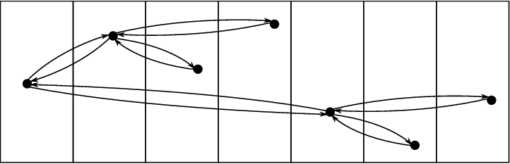
Appendix 0.B Proofs of Statements from Sections 1,4 and 5
Proof of equations 1, 2 and 3
The relation comes from our Theorem 4.1. The fact that is implied by together with . Finally is implied by together with . We observe that we are not aware of a generalization of the well known inequality , relating undirected path-width to undirected tree-width, to the directed setting. In other words we do not know whether . Such a generalization would imply .
Proof of Corollary 1
We start from item : Robertson and Seymour’s graph minor Theorem states that any minor closed graph property is characterized by a finite set of forbidden minors [23]. The non-existence of each minor in can be expressed by a monadic second order formula (See for example [14]); The properties in items are all closed under minors, and therefore, by Item there is a monadic second order formula expressing each of these properties. : Clearly there exists a formula expressing connectedness, namelly, that there is a path between any two vertices. A graph is bipartite if and only if it has no cycle of odd length, which is also easy to express in MSOL.
Appendix 0.C Proofs of Results from Section 7
Proposition 3
Let be a digraph, and be a -topological ordering of of cut width .
- 1.
If is a subgraph of and is the restriction of to the vertices of , then
- (a)
has cut-width at most w.r.t. .
- (b)
is a -topological ordering of .
- (a)
- 2.
The zig-zag number is at most the cut-width .
- 3.
If is any digraph with same set of vertices as and if has cut-width with respect to then has cut-width at most with respect to .
- 4.
Let be a set of not necessarily edge disjoint nor vertex disjoint paths of such that . Then .
Proof
1a) Since has cut width with respect to , we have that there are at most edges with one endpoint in and other endpoint in for each with . Therefore there are at most edges with one endpoint in and other endpoint in for each such an . Implying in this way that has cut-width at most w.r.t the ordering induced by . 1b) Since is a -topological ordering of , any path of has cut-width at most w.r.t. the restriction of to the vertices of . Since any path of is a sub-path of some path of , by item 1.a has cut-width at most with respect to the ordering induced by (and consequently by ) on the vertices of . 2) The proof is by contradiction. Suppose . Then there exists a path in that has cut-width with respect to the restriction of to the vertices of . Since is a subgraph of , by item , contradicting the assumption that . 3) For any such that , there exist at most edges of with one endpoint in and other endpoint in . Analogously there are at most edges of with one endpoint in and other endpoint in . Therefore there are at most edges of with one endpoint in and other endpoint in for each such an . Thus has cut-width at most . 4) Since is a -topological ordering of , each path of has cut-width at most with respect to . Since for paths , by item 3 of this proposition, .
Proposition 4 (Counting Paths in a DAG)
Let be a DAG on vertices and let and be two arbitrary subsets of . Then one may count the number of distinct simple paths from to in time .
Proof
We start by adding a vertex to and connecting it to each vertex in . Similarly, we add a vertex to and add a directed edge from each vertex in to . We will assign weights for each vertex of . For each , the weight will count the number of paths from to . Indeed we will define a sequence of functions which will converge to when is greater or equal to the height of , i.e., the size of the longest path from to . Initially, we will set and for all other vertices in . Subsequently, for each , let be the set of all forward neighbors of . Then set for . By induction on the height of , we have that for each , the weight represents precisely the number of simple paths from to . In particular represents the number of simple paths from to which is equal to the number of simple paths from to . Therefore, let for each .
Proof of Proposition 2
The inclusion holds for any two slice languages and irrespectively of whether they are saturated or not: Let be a digraph in . Then has a unit decomposition in . Since , and, since , . Thus . Now we prove that if is saturated the converse inclusion also holds: Let be a digraph in . Since has zig-zag number , there exists a unit decomposition of of zig-zag number in . Since is -saturated any unit-decomposition of of zig-zag number at most is in , and in special . Therefore and .
Proof of Lemma 1
The slice graph is constructed as follows: For each slice (recall again that belongs to not in , and that ) we let be the set of all numbered sub-slices of of slice-width at most (Figure 2.), including slices with empty in-frontier, empty out-frontier or both (this last case embraces both the empty slice and slices with a unique vertex in the center and no frontier vertex). We should pay attention to the fact that the numbering of the frontier vertices of each such a subslice is inherited from the numbering of , as illustrated in figure 2., and thus these subslices are not necessarily normalized. This observation is crucial and will play a role in the fact that is deterministic. For each such a sub-slice (now ) we add a vertex to and label it with (i.e., ). Subsequently we add an edge if and only if and if can be glued to respecting the numbering of the touching-frontier vertices. Observe that a slice with empty out-frontier can always be glued to a slice with an empty in-frontier. This last observation allows us to represent some unit decompositions of disconnected sub-graphs. The initial vertices in are the vertices labeled with the sub-slices of with empty in-frontier (including the empty slice), while the terminal vertices in are those labeled with slices from with empty out-frontier. We observe that all the dilated sub-unit-decompositions generated by will have length , irrespectively of the size of the subgraph of that each of them represents. Therefore each such a sub-unit decompositions will be potentially padded with sequences of empty slices to its left and right. Now it should be clear that a sequence is a sub-unit decomposition of if and only if there exists a sequence labeled with . Therefore the slice language represents precisely the set of sub-unit decompositions of of slice-width at most . As mentioned above, is deterministic. This fact is guaranteed by the fact that even if a vertex in has two forward neighbors labeled with slices carrying the same structure, their frontiers will forcefully have distinct numberings, and thus will be considered different. Finally, the construction we just described can be realized in time since there are at most subslices of each slice and we only connect vertices in labeled with neighboring subslices.
Proposition 5
Let be a slice graph. Then a dilated unit decomposition belongs to if and only if the unit decomposition
belongs to for a set of pairs of functions where is a -numbering of .
Proof of Theorem 7.1
Let be a digraph on vertices and assume that is a subgraph of which is isomorphic to a digraph in . Since is a subgraph of , there is a dilated unit decomposition that is a sub-unit decomposition of . By Proposition 1., has zig-zag number at most , and therefore is compatible with some -topological ordering of of the vertices of . Now notice that the slices are not normalized. Therefore there exist a normalized unit decomposition of such that for some -numbering of . Since is dilated saturated, and also has zig-zag number , we have that . Thus by Proposition 5, , and therefore .
Conversely, assume that the numbered dilated unit decomposition
of the digraph belongs to the slice language . Then by proposition 5, the unit decomposition belongs to and since is also a unit decomposition of , we have that . Since by Lemma 1 all unit decompositions in are sub-unit decompositions of we have that is a subgraph of . Therefore is a subgraph of isomorphic to a digraph in .
Appendix 0.D Proof Of Theorem 8.1
In the composition of slices defined in Section 6, both the out-frontier vertices of and the in-frontier vertices of disappear, since they are not meant to be part of the structure of the composed graph. In this section however, it will be more convenient to consider a slightly different composition of slices. In this composition, which we denote by we simply add an edge from each out-frontier vertex of to its corresponding equally numbered in-frontier vertex in . Indeed we will represent the existence of such an edge by a predicate which will be true whenever belongs to the out-frontier of a slice , belongs to the in-frontier of a consecutive slice and they have the same number. By consecutive slices we mean two slices that appear in consecutive positions in a slice string. We notice that the edge relation of graphs that arise by gluing slices according to the first composition can be recovered from the edge relation of the graphs that arise if they were composed using . More precisely, let and . Then we define the formula to be true if and only if is the set of edges of a path in such that , is not a frontier vertex, and holds for every with . Analogously, is true if is the set of edges of a path in which , is not a frontier vertex and for all all intermediary vertices with . The existence of such a path can easily be expressed in . Observe that the way in which slices are composed and the way in which slice graphs are defined will guarantee that for any two non-frontier vertices there exists at most one path such that all intermediary vertices are frontier vertices. Therefore each edge in will correspond to exactly one such a path in and vice versa. Analogously, the relations and can be easily simulated in terms of formulas involving and .
Without loss of expressiveness, one may eliminate the need to quantify over first order variables [46]. This will be in useful to reduce the number of special cases in the proof of Lemma 2 below. The trick is to simulate first order variables via a second order predicate which is interpreted as true whenever and as false otherwise. To avoid a cumbersome notation, whenever we refer to a variable as being a single vertex or edge, we will assume that is true. Since we will deal with slices, it will also be convenient to have in hands a relation which is true if and only if represents a frontier vertex, and a relation which is true if and represent vertices in the same frontier of a slice. More formally, let be a set of vertex labels, be a set of edge labels, be an infinite set of second order variables ranging over sets of vertices and let denote a formula with free variable . Then the set of formulas over directed graphs is the smallest set of formulas containing:
- •
the atomic formulas, , , , , , , for each , for each ,
and ; - •
the formulas , , and , where and are formulas.
Now we follow an approach that is similar to that used in [46, 37] but lifted in such a way that it will work with slices. Let be a formula with free second order variables and be a unit slice with vertices and edges (including the frontier vertices). We represent an interpretation of in as a boolean matrix whose rows are indexed by the variables in and the columns are indexed by the vertices and edges of . Intuitively, we set if and only if the vertex or edge of corresponding to the -th column of belongs to the -th variable of . In this setting a sequence of interpretations of a unit decomposition , in which is an interpretation of , provides a full interpretation of the graph . Let be the slice alphabet of width . We define the interpreted extension of to be the alphabet
Now we are in a position to prove Lemma 2. For each formula over a set of free variables we will define a regular subset of the free monoid generated by satisfying the following property: A string
belongs to if and only if the digraph satisfies with interpretation .
Proof of Lemma 2
Proof
By the discussion above we start by replacing each occurrence of the atomic formulas , , … in by the atomic formulas , ,… so that we can reason in terms of the composition instead of in terms of the composition . Let . First we will construct a finite automaton which accepts precisely the interpreted strings
for which with interpretation of over . The proof is by induction on the structure of the formula. It is easy to see that the atomic formulas , , , , , for each and , can be checked by a finite automaton. For instance, to check whether holds in , the automaton verifies for each interpretation with and for each column of , that whenever then . To determine whether (or ) is true, first check whether are singletons. If this is not the case, reject. Otherwise let be interpreted as and as . Then accept either if and belong to the same slice and if , which can be done by table lookup. To determine whether is true, check whether and are singletons, , belongs to the out-frontier of a slice and to the in-frontier of a consecutive slice. Disjunction, conjunction and negation are handled by the fact that DFAs are effectively closed under union, intersection and complement. In other words,
| (6) |
To eliminate existential quantifiers we proceed as follows: For each variable , define the projection that sends each symbol to the symbol in where denotes the matrix with the row corresponding to the variable deleted. Extend homomorphically to strings by applying it coordinatewise, and subsequently to languages by applying it stringwise. Then set
Notice that even though homomorphisms in general do not preserve regularity, in the case of projections of symbols as defined above, this is not an issue. In particular one can obtain a DFA accepting from a DFA accepting by simply replacing each symbol appearing in a transition of by the symbol . At the end of this inductive process, all variables will have been projected, since is a sentence. Thus the language will accept precisely the slice strings whose composition yield a digraph that satisfies . As a last step in our construction, we eliminate illegal sequences of slices, from the language generated by our constructed automaton, we intersect it with another automaton that rejects precisely the sequences of slices in which two slices that cannot be composed appear in consecutive positions.
For a matter of clarity, from now on we will relax our language and use lower case letters whenever referring to single edges and vertices. Let the predicate be true whenever is the set of vertices of some path, be true whenever is the set of edges of some path and the be true whenever is the set of vertices and the set of edges of the same path. Then the fact that a unit decomposition has zig-zag width at most can be expressed in as
Basically it says that if is the set of vertices of a path and if are vertices in this path then at least two of them belong to different frontiers. We say that a digraph is -path-unitable if there is a set of not necessarily edge disjoint nor vertex disjoint paths such that . The fact that a graph is -path-unitable can be expressed by the formula
Proof of Theorem 8.1
Let . By Lemma 2, there is a regular slice language over generating all unit decompositions over whose composition yields a graph satisfying , and in particular . Since the factor is present in all these graphs can be cast as the union of -paths. Since the factor is present in , all unit decompositions in have zig-zag number at most . It remains to show that every unit decomposition of zig-zag number at most of a graph is in . This follows from the fact that is the union of directed paths, and from Proposition 3.4 stating that any unit decomposition of zig-zag number at most of a digraph that is the union of at most directed paths has slice-width at most . Thus is -saturated. To finish the proof set as any slice graph generating