Finding all convex cuts of a plane graph in polynomial time

Parts of this paper have been published in a preliminary form in Proceedings of the 8th International Conference on Algorithms and Complexity (CIAC’13) [12].

Roland Glantz, Henning Meyerhenke ^†^†thanks: Homepage: http://parco.iti.kit.edu/glantz/^†^†thanks: Homepage: http://parco.iti.kit.edu/henningm/ Affiliation: Institute of Theoretical Informatics Affiliation: Karlsruhe Institute of Technology (KIT) Affiliation: Karlsruhe, Germany

Abstract

Convexity is a notion that has been defined for subsets of $\mathbb{R}^{n}$ and for subsets of general graphs. A convex cut of a graph $G=(V,E)$ is a $2$ -partition $V_{1}\dot{\cup}V_{2}=V$ such that both $V_{1}$ and $V_{2}$ are convex, i. e., shortest paths between vertices in $V_{i}$ never leave $V_{i}$ , $i\in\{1,2\}$ . Finding convex cuts is $\mathcal{NP}$ -hard for general graphs. To characterize convex cuts, we employ the Djoković relation, a reflexive and symmetric relation on the edges of a graph that is based on shortest paths between the edges’ end vertices.

It is known for a long time that, if $G$ is bipartite and the Djoković relation is transitive on $G$ , i. e., $G$ is a partial cube, then the cut-sets of $G$ ’s convex cuts are precisely the equivalence classes of the Djoković relation. In particular, any edge of $G$ is contained in the cut-set of exactly one convex cut. We first characterize a class of plane graphs that we call well-arranged. These graphs are not necessarily partial cubes, but any edge of a well-arranged graph is contained in the cut-set(s) of at least one convex cut. Moreover, the cuts can be embedded into the plane such that they form an arrangement of pseudolines, or a slight generalization thereof. Although a well-arranged graph $G$ is not necessarily a partial cube, there always exists a partial cube that contains a subdivision of $G$ .

We also present an algorithm that uses the Djoković relation for computing all convex cuts of a (not necessarily plane) bipartite graph in $\mathcal{O}(|E|^{3})$ time. Specifically, a cut-set is the cut-set of a convex cut if and only if the Djoković relation holds for any pair of edges in the cut-set.

We then characterize the cut-sets of the convex cuts of a general graph $H$ using two binary relations on edges: (i) the Djoković relation on the edges of a subdivision of $H$ , where any edge of $H$ is subdivided into exactly two edges and (ii) a relation on the edges of $H$ itself that is not the Djoković relation. Finally, we use this characterization to present the first algorithm for finding all convex cuts of a plane graph in polynomial time.

Keywords: Convex cuts, Djoković relation, partial cubes, plane graphs, bipartite graphs

1 Introduction

A convex $k$ -partition of an undirected graph $G=(V,E)$ is a partition $(V_{1},\dots,V_{k})$ of $V$ such that the subgraphs of $G$ induced by $V_{1},\dots V_{k}$ are all convex. A convex subgraph of $G$ , in turn, is a subgraph $S$ of $G$ such that for any pair of vertices $v,w$ in $S$ all shortest paths from $v$ to $w$ in $G$ are fully contained in $S$ . The vertex set of a convex subgraph is called convex set.

A convex cut of $G$ is a convex $2$ -partition of $G$ . If $G$ has a convex $k$ -partition, then $G$ is said to be $k$ -convex. Artigas et al. [1] showed that, for a given $k\geq 2$ , it is $\mathcal{NP}$ -complete to decide whether a (general) graph is $k$ -convex. Moreover, given a bipartite graph $G=(V,E)$ and an integer $l<|V|$ , it is $\mathcal{NP}$ -complete to decide whether there exists a convex set with at least $l$ vertices [10].

There exists a different notion of convexity for plane graphs. A plane graph is called convex if all of its faces are convex polygons. This second notion is different and not object of our investigation. The notion of convexity in acyclic directed graphs, motivated by embedded processor technology, is also different [2]. There, a subgraph $S$ is called convex if there is no directed path between any pair $v,w$ in $S$ that leaves $S$ . In addition to being directed, these paths do not have to be shortest paths as in our case.

Applications that potentially benefit from convex cuts include data-parallel numerical simulations on graphs. Here the graph is partitioned into parts that have nearly the same number of vertices [3, 5]. For some linear solvers used in these simulations, the shape of the parts, in particular short boundaries, small aspect ratios, but also connectedness and smooth boundaries, plays a significant role [13]. Convex subgraphs of meshes typically admit these properties. Another example is the preprocessing of road networks for shortest path queries by partitioning according to natural cuts [7]. The definition of a natural cut is not as strict as that of a convex cut, but they have a related motivation.

Due to the importance of graph partitions in theory and practice [3], it is natural to ask whether the time complexity of finding convex cuts is polynomial for certain types of input graphs. In this paper, we will see that polynomial-time algorithms exist for a sub-class of plane graphs and for bipartite graphs. Specifically, a cut-set is the cut-set of a convex cut of a bipartite graph if and only if the Djoković relation holds for any pair of edges in the cut-set.

We also characterize the cut-sets of the convex cuts of a general graph $H$ in terms of two binary relations, each on a different kind of edges: the edges of a subdivision of $H$ , where any edge of $H$ is subdivided into two edges and (ii) the edges of $H$ itself. The relation on the first kind of edges is the Djoković relation (see Section 2), and the relation on the second kind of edges, denoted by $\tau$ , is such that $e~\tau~f$ iff the distance between any end vertex of $e$ to any end vertex of $f$ is the same.

1.1 Related work

Artigas et al. [1] show that every connected chordal graph $G=(V,E)$ is $k$ -convex, for $1\leq k\leq|V|$ . They also establish conditions on $|V|$ and $p$ to decide whether the $p$ th power of a cycle is $k$ -convex. Moreover, they present a linear-time algorithm that decides whether a cograph is $k$ -convex.

Our methods for characterizing and finding convex cuts of a plane graph $G$ are motivated by the work in Chepoi et al. [6] who defined alternating cuts and specified conditions under which alternating cuts are convex cuts and vice versa. Our approach is more myopic, though. We call a face $F$ of $G$ even [odd] if $|E(F)|$ is even, and an alternating path is one that cuts an even face $F$ such that the number of vertices in the two parts of $E(F)$ is equal. In an odd face the alternating path makes a slight left or right turn so that the number of vertices in the two parts of $E(F)$ differ by one. As in [6], when following an alternating path through the faces of $G$ , a left [right] turn must be compensated by a right [left] turn as soon as this is possible.

Plane graphs usually have alternating cuts that are not convex and convex cuts that are not alternating. Proposition 2 in [6] characterizes the set of plane graphs for which the alternating cuts coincide with the convex cuts in terms of a condition on the boundary of any alternating cut. In this paper we represent the alternating cuts as plane curves that we call embedded alternating paths (EAPs)—an EAP partitions $G$ exactly like the alternating cut it represents. In contrast to [6], however, we focus on the intersections of the EAPs (i. e., alternating cuts).

If any pair of EAPs intersects at most once, we have a slight generalization of what is known as an arrangement of pseudolines. The latter arise in discrete geometry, computational geometry, and in the theory of matroids [4]. Duals of arrangements of pseudolines are known to be partial cubes (see Section 2), a fact that has been applied to graphs before by Eppstein [11], for example. For basics on partial cubes we rely on Ovchinnikov’s survey [14]. The following basic fact about partial cubes is crucial for our method to find convex cuts: partial cubes are precisely the graphs that are bipartite and on which the Djoković relation [9] (defined in Section 2) is transitive. For a characterization of planar partial cubes see Peterin [15].

1.2 Paper outline and contribution

In Section 3 we first represent (myopic versions of) the alternating cuts of a plane graph $G=(V,E)$ , as defined in [6], by EAPs. The main work here is on the proper embedding. We then study the case of $G$ being well-arranged, as we call it, i. e., the case in which the EAPs form an arrangement of pseudolines, or a slight generalization thereof. We show that the dual ${G}_{\mathcal{E}}$ of such an arrangement is a partial cube and reveal a one-to-one correspondence between the EAPs of $G$ and the convex cuts of ${G}_{\mathcal{E}}$ . Specifically, the edges of ${G}_{\mathcal{E}}$ intersected by an EAP form the cut-set of a convex cut of ${G}_{\mathcal{E}}$ . Conversely, the cut-set of any convex cut of ${G}_{\mathcal{E}}$ is the set of edges intersected by a unique EAP of $G$ . From (i) the one-to-one correspondence between the EAPs of $G$ and the convex cuts of ${G}_{\mathcal{E}}$ and (ii) the construction of ${G}_{\mathcal{E}}$ we derive that the EAPs also define convex cuts of $G$ .

In Section 4 we specify an $\mathcal{O}(|E|^{3})$ -time algorithm to find all convex cuts of a not necessarily plane bipartite graph. The fact that we can compute all convex cuts in bipartite graphs in polynomial time is no contradiction to the $\mathcal{NP}$ -completeness of the decision problem whether the largest convex set in a bipartite graph has a certain size [10]. Indeed, for a cut to be convex, both subgraphs have to be convex, whereas the complement of a convex set is not required to be a convex set itself.

In Section 5 we characterize the cut-sets of the convex cuts of a general graph $H$ in terms of the Djoković relation and $\tau$ . The results of Section 5 are then used in Section 6 to derive new necessary conditions for convexity of cuts of a plane graph $G$ . As in the case of well-arranged graphs, we iteratively proceed from an edge on the boundary of a face $F$ of $G$ to another edge on the boundary ”opposite“ of $F$ . This time, however, “opposite” is with respect to the Djoković relation on a subdivision of $G$ . Thus we arrive at a polynomial-time algorithm that finds all convex cuts of $G$ . We correct an error in a preliminary version [12] of this paper. The running time is now $\mathcal{O}(|V|^{7})$ instead of $\mathcal{O}(|V|^{3})$ .

2 Preliminaries

Unless stated otherwise, $G=(V,E)$ is a finite, undirected, unweighted, and two-connected graph that is free of self-loops. Two-connectedness is not a limitation for the problem of finding convex cuts because a convex cut cannot cut through more than one block of $G$ , and self-loops have no impact on the convex cuts. For $e\in E$ with end points $u,v$ ( $u\not=v$ ) we sometimes write $e=\{u,v\}$ even when $e$ is not necessarily determined by $u$ and $v$ due to parallel edges. We use the term path in the general sense: a path does not have to simple, and it can be a cycle.

If $G$ is plane, $V$ is a set of points in $\mathbb{R}^{2}$ , and $E$ is a set of plane curves that intersect only at their end points which, in turn, make up $V$ . The unbounded face of $G$ is denoted by $F_{\infty}$ . For a face $F$ of $G$ , we write $E(F)$ for the set of edges that bound $F$ . Our definitions and results on plane graphs are invariant to topological isomorphism [8] which, in conjunction with two-connectedness, is equivalent to combinatorial isomorphism [8]. Since any plane graph is combinatorially isomorphic to a plane graph whose edges are line segments [8], we can always resort to the case of straight edges without loss of generality. We do so especially in our illustrations.

We denote the standard metric on $G$ by $d_{G}(\cdot,\cdot)$ . In this metric the distance between $u,v\in V$ amounts to the number of edges on a shortest path from $u$ to $v$ . A subgraph $S=(V_{S},E_{S})$ of a (not necessarily plane) graph $H$ is an isometric subgraph of $H$ if $d_{S}(u,v)=d_{H}(u,v)$ for all $u,v\in V_{S}$ .

Following Djoković [9] and using Ovchinnikov’s notation [14], we set

W_{xy}=\{w\in V:d_{G}(w,x)<d_{G}(w,y)\}\quad\forall\{x,y\}\in E.

(1)

Let $e=\{x,y\}$ and $f=\{u,v\}$ be two edges of $G$ . The Djoković relation $\theta$ on $G$ ’s edges is defined as follows:

e~\theta~f\Leftrightarrow f\mbox{~has one end vertex in $W_{xy}$ and one in $W_{yx}$}.

(2)

The Djoković relation is reflexive, symmetric [17], but not necessarily transitive. The vertex set $V$ of $G$ is partitioned by $W_{ab}$ and $W_{ba}$ if and only if $G$ is bipartite.

A partial cube $G_{q}=(V_{q},E_{q})$ is an isometric subgraph of a hypercube. Interested readers find more details on partial cubes in Ovchinnikov’s survey [14]; we state a few important results for the sake of self-containment. Partial cubes and $\theta$ are related in that a graph is a partial cube if and only if it is bipartite and $\theta$ is transitive. Thus, $\theta$ is an equivalence hypercube. For a survey on partial cubes see Ovchinnikov [14]. Partial cubes and $\theta$ are related in that a graph is a partial cube if and only if it is bipartite and $\theta$ is transitive. Thus, $\theta$ is an equivalence relation on $E_{q}$ , and the equivalence classes are cut-sets of $G_{q}$ . Moreover, the cuts defined by these cut-sets are precisely the convex cuts of $G_{q}$ . If $(V_{q}^{1},V_{q}^{2})$ is a convex cut, the (convex) subgraphs induced by $V_{q}^{1}$ and $V_{q}^{2}$ are called semicubes. If $\theta$ gives rise to $k$ equivalence classes $E_{q}^{1},\dots E_{q}^{k}$ , and thus $k$ pairs $(S_{a}^{i},S_{b}^{i})$ of semicubes, where the ordering of the semicubes in the pair is arbitrary, one can derive a Hamming labeling $b:V_{q}\mapsto\{0,1\}^{k}$ by setting

b(v)_{i}=\left\{\begin{array}[]{ll}0&\quad\mbox{if $v\in S_{a}^{i}$}\\ 1&\quad\mbox{if $v\in S_{b}^{i}$}\end{array}\right.

(3)

In particular, $d_{G_{q}}(u,v)$ amounts to the Hamming distance between $b(u)$ and $b(v)$ for all $u,v\in V_{q}$ . This is a consequence of the fact that the corners of a hypercube have such a labeling and that $G_{q}$ is an isometric subgraph of a hypercube.

3 Partial cubes from embedding alternating paths

In Section 3.1 we define a multiset of (not yet embedded) alternating paths of a graph $G$ . Section 3.2 is devoted to embedding the alternating paths into $\mathbb{R}^{2}$ and to the definition of well-arranged graphs. In Section 3.3 we study the dual of an embedding of alternating paths and show that it is a partial cube whenever $G$ is well-arranged.

3.1 Alternating paths

Intuitively, an embedded alternating path $P$ runs through a face $F$ of $G$ such that the edges through which $P$ enters and leaves $F$ are opposite—or nearly opposite because, if $|E(F)|$ is odd, there is no opposite edge, and $P$ has to make a slight turn to the left or to the right. The exact definitions leading up to (not yet embedded) alternating paths are as follows.

Definition 3.1 (Opposite edges, left, right, unique opposite edge).

Let $F\not=F_{\infty}$ be a face of $G$ , and let $e,f\in E(F)$ . Then $e$ and $f$ are called opposite edges of $F$ if the lengths of the two paths induced by $E(F)\setminus\{e,f\}$ differ by at most one. If the two paths have different lengths, $f$ is called the left [right] opposite edge of $e$ if starting on $e$ and running clockwise around $F$ , the shorter [longer] path comes first. Otherwise, $e$ and $f$ are called unique opposite edges.

Definition 3.2 (Alternating path graph $A(G)=(V_{A},E_{A})$ ).

The alternating path graph $A(G)=(V_{A},E_{A})$ of $G=(V,E)$ is the (non-plane) graph with $V_{A}=E$ and $E_{A}$ consisting of all two-element subsets $\{e,f\}$ of $E$ such that $e$ and $f$ are opposite edges of some face $F\not=F_{\infty}$ .

The alternating path graph defined above will provide the edges for the multiset of alternating paths defined next. We resort to a multiset for the sake of uniformity, i.e., to ensure that any edge of $G$ is contained in exactly two alternating paths (see Figure 1a).

Refer to caption — Figure 1: Primal graph: black vertices, thin solid edges. Dual graph: white vertices, dashed edges. (a) Multiset $\mathcal{P}(G)$ of alternating paths: Red vertices, thick solid lines. The paths in $\mathcal{P}(G)$ are colored. In this ad-hoc drawing the two alternating paths that share a vertex, i. e., an edge of $G$ , go through the same (red) point on the edge. (b) Collection $\mathcal{E}(G)$ of EAPs: Red vertices, thick solid colored lines.

Definition 3.3 ((Multiset $\mathcal{P}(G)$ of) alternating paths in $A(G)$ ).

A maximal path $P=(v_{A}^{1},e_{A}^{1},v_{A}^{2},\dots e_{A}^{n-1},v_{A}^{n})$ in $A(G)=(V_{A},E_{A})$ is called alternating if

(i)

$v_{A}^{i}$ and $v_{A}^{i+1}$ are opposite for all $1\leq i\leq n-1$ and
(ii)

if $v_{A}^{i+1}$ is the left [right] opposite of $v_{A}^{i}$ , and if $j$ is the minimal index greater than $i$ such that $v_{A}^{j}$ and $v_{A}^{j+1}$ are not unique opposites (and $j$ exists at all), then $v_{A}^{j+1}$ is the right [left] opposite of $v_{A}^{j}$ .

We (arbitrarily) select one path from each pair formed by an alternating path $P$ and the reverse of $P$ . The multiset $\mathcal{P}(G)$ contains all selected paths: the multiplicity of $P$ in $\mathcal{P}(G)$ is two if $v_{A}^{i+1}$ is a unique opposite of $v_{A}^{i}$ for all $1\leq i\leq n-1$ , and one otherwise.

3.2 Embedding of alternating paths

In this section we embed the alternating paths of a plane graph $G$ into $\mathbb{R}^{2}$ . We may assume that the edges of $G$ are straight line segments (see Section 2). An edge $\{e,f\}$ of an alternating path turns into a non-self-intersecting plane curve with one end point on $e$ and the other end point on $f$ . An alternating path with multiplicity $m\in\{1,2\}$ gives rise to $m$ embedded paths. Visually, we go from Figure 1a to Figure 1b.

Note that any edge $e$ of $G$ is contained in exactly two alternating paths. For any $e$ that separates two bounded odd faces we predetermine a point $s$ on $e$ ’s interior and require that both alternating paths containing $e$ must run through $s$ . If $e$ does not separate two odd faces, we predetermine two points, $s_{1}$ and $s_{2}$ , on $e$ ’s interior and require that one alternating path runs through $s_{1}$ and the other one runs through $s_{2}$ . We refer to $s$ , $s_{1}$ and $s_{2}$ as slots of $e$ . If $P=(v_{A}^{1},e_{A}^{1},v_{A}^{2},\dots e_{A}^{n-1},v_{A}^{n})$ is an alternating path, let $F_{i}=F_{i}(P)$ be the $i$ th (bounded) face of $G$ that will be traversed by embedded $P$ , i. e., the (unique) face with $v_{A}^{i},v_{A}^{i+1}\in E(F_{i})$ . Since we required that $G$ is two-connected, we have $v_{A}^{i}\neq v_{A}^{i+1}$ . Thus, if $v_{A}^{i}$ has two slots, there exists a well-defined left and right slot from the perspective of standing on $v_{A}^{i}$ and looking into $F_{i}$ , $1\leq i<n$ . Finally, left and right on $v_{A}^{n}$ is from the perspective of looking into $F_{\infty}$ .

The overall scenario is that we embed the alternating paths one after the other, where the order of the paths is arbitrary. The following rules for an individual path $P$ then determine which slots are occupied by which alternating paths. For an example of slot choice see Figure 2a,b. The variable $a(P)$ is zero if and only if $P$ makes no left and no right turn. Otherwise, $a(P)$ indicates the preference for the next slot at any time.

1.

If $P$ has no left turn and no right turn, set $a(P)$ to $0$ . Otherwise, if the first turn of $P$ is a left [right] turn, set $a(P)$ to $l$ [ $r$ ].
2.

Let $s_{l}$ [ $s_{r}$ ] be the left [right] slot on $v_{A}^{1}$ . If $a(P)=0$ , choose a vacant slot (arbitrarily if both slots are vacant). If $a(P)=l$ [ $a(P)=r$ ], occupy the left [right] slot if that slot is still vacant. Otherwise, occupy the alternative slot and set $a(P)=r$ [ $a(P)=l$ ].
3.

Assume that we have found slots for $v_{A}^{1},\dots v_{A}^{i}$ .
- •
  
  If $a(P)=0$ and the slot occupied on $v_{A}^{i}$ was the left [right] slot, then occupy the left [right] slot on $v_{A}^{i+1}$ .
- •
  
  If $v_{A}^{i+1}$ has only one slot, then occupy it (single slots can be occupied by two paths). If $(a(P)=l)$ [ $(a(P)=r)$ ], then set $(a(P)=r)$ , [ $(a(P)=l)$ ].
- •
  
  If $v_{A}^{i+1}$ has two slots and $a(P)=l$ [ $a(P)=l$ ], then occupy the left [right] slot, if vacant. Otherwise, occupy the alternative slot and set $a(P)=r$ [ $a(P)=l$ ].

The embedding of the alternating paths will be such that two paths that share a point $p$ will always cross at $p$ , and not just touch (see Proposition 3.4 and Figure 2c). We are not interested in the exact course of the embedded alternating paths (EAPs), but only in their intersection pattern, i. e., whether certain pairs of EAPs cross in a certain face or on a certain edge. The intersection pattern is not going to be unique, but our central definition, i. e., that of a well-arranged graph, will be invariant to ambiguities of intersection patterns (see Proposition 3.6).

Next we formulate rules for embedding a single edge $\{e,f\}$ of an alternating path into $\mathbb{R}^{2}$ . If $F$ is the unique face of $G$ with $\{e,f\}\subset E(F)$ , we embed $\{e,f\}$ into $\overline{F}=F\cup E(F)$ . To this end, we first represent $\overline{F}$ by a regular filled polygon $\overline{F_{r}}$ with the same number of sides. We then embed $\{e,f\}$ into $\overline{F_{r}}$ as a line segment $L$ between two points on the sides of $\overline{F_{r}}$ . Due to the Jordan-Schönflies theorem [16], there exists a homeomorphism $\hslash:\overline{F_{r}}\mapsto\overline{F}$ . The embedding of $\{e,f\}$ into $\overline{F}$ is then given by $\hslash(L)$ . Since $\hslash$ is a homeomorphism, the intersection pattern of the line segments in $\overline{F}$ coincides with that in $\overline{F_{r}}$ (see Figures 3a and 4a).

Local embedding rules. The local rules for embedding an alternating path into $\overline{F_{r}}$ are as follows.

1.

The part of an EAP that runs through $F_{r}$ is a line segment, and EAPs cannot coincide in $F_{r}$ .
2.

An EAP can intersect $e\in E(F_{r})$ only in $e$ ’s relative interior, i. e., not at $e$ ’s end vertices.
3.

Let $F_{r}\not=F_{\infty}$ be an even face of $G$ , let $e,f$ be unique opposite edges in $E(F_{r})$ , and let $P_{1},P_{2}$ be the two alternating paths that contain the edge $\{e,f\}$ ( $P_{1}=P_{2}$ if and only if the multiplicity of $P_{1}$ is two). Then the parts of embedded $P_{1}$ and $P_{2}$ that run through $\overline{F_{r}}$ must form a pair of distinct parallel line segments (see Figure 3a).
4.

Let $F\not=F_{\infty}$ be an odd face of $G$ , let $e\in E(F_{r})$ , and let $P_{1},P_{2}$ be the two alternating paths that contain the vertex $e$ . If $e$ also bounds an even bounded face or $F_{\infty}$ , embedded $P_{1},P_{2}$ must intersect $e$ at two distinct points (see the upper left edge of the hexagon in Figures 3b,c). If the other face is a bounded odd face, embedded $P_{1},P_{2}$ must cross at a point on $e$ (see the upper right edge of the hexagon in Figures 3b,c).
5.

A slot conflict on an edge $e$ of $G$ can occur only if $e$ separates a bounded odd face $F$ from a face that is not both bounded and odd. Let $\{e,f\}$ , $\{e,f^{\prime}\}$ be the two edges (of alternating paths) occupying the two slots of $e$ , and let $F_{r}$ be the regular polygon that represents $F$ . Then $\{e,f\}$ and $\{e,f^{\prime}\}$ cross inside $F_{r}$ if and only if there is a slot conflict on $e$ (see Figures 3b,c).

We map the embedded edges (of alternating paths) from any $\overline{F_{r}}$ into $\overline{F}$ using a homeomorphism from $\overline{F_{r}}$ onto $\overline{F}$ . The following is about tying the loose ends of the locally embedded paths, which all sit on edges of $G$ , so as to arrive at a global embedding of the alternating paths (see Figures 4b,c). Let $e\in E(G)$ , and let $F,F^{\prime}$ be the faces of $G$ that are bounded by $e$ . We have two locally embedded paths $P_{F}^{1},P_{F}^{2}$ in $\overline{F}$ and two locally embedded paths $P_{F^{\prime}}^{1},P_{F^{\prime}}^{2}$ in $\overline{F^{\prime}}$ that all hit $e$ . We bend the four paths toward their predetermined slots. The bending operations can be done such that the intersection patterns do not change in the interiors of $F$ and $F^{\prime}$ . Indeed, recall that the paths are homeomorphic to straight line segments. Thus, there exists $\epsilon>0$ such that all locally embedded paths in $F$ and $F^{\prime}$ other than $P_{F}^{1}$ , $P_{F}^{2}$ , $P_{F^{\prime}}^{1}$ , and $P_{F^{\prime}}^{2}$ keep a distance greater than $\epsilon$ to $e$ . The bending, in turn, can be done such that it affects $P_{F}^{1}$ , $P_{F}^{2}$ , $P_{F^{\prime}}^{1}$ , and $P_{F^{\prime}}^{2}$ only in an $\epsilon$ -neighborhood of $e$ .

Proposition 3.4.

If two EAPs share a point $p$ , they cross at $p$ and not just touch.

Proof.

Consider two EAPs $P_{1}$ and $P_{2}$ that share a point $p$ . If $p$ sits in a face $F$ of $G$ , $P_{1}$ and $P_{2}$ cross at $p$ because (i) $P_{1}=\hslash(L_{1})$ and $P_{2}=\hslash(L_{2})$ for a homeomorphism $\hslash:F_{r}\mapsto F$ , (ii) $L_{1}\not=L_{2}$ cannot touch without crossing, and (iii) homeomorphisms preserve crossings and non-crossings of curves.

If $p$ sits on (the interior of an edge) $e\in E$ , the two faces separated by $e$ , and denoted by $F$ and $F^{\prime}$ , must be finite and odd. As illustrated in Figure 2c, $P_{1}$ [ $P_{2}$ ] enters $F$ through an edge $e_{F}^{1}$ [ $e_{F}^{2}$ ] in $E(F)\setminus E(F^{\prime})$ , runs from $F$ into $F^{\prime}$ via $e$ , and then leaves $F^{\prime}$ via an edge $e_{F^{\prime}}^{1}$ [ $e_{F^{\prime}}^{2}$ ] in $E(F^{\prime})\setminus E(F)$ . Since $F$ and $F^{\prime}$ are finite and odd, we have $e_{F}^{1}\neq e_{F}^{2}$ and $e_{F^{\prime}}^{1}\neq e_{F^{\prime}}^{2}$ . Without loss of generality, $e$ is the left [right] opposite of $e_{F}^{1}$ [ $e_{F}^{2}$ ]. Then, due to item (ii) in Definition 3.3, $e_{F^{\prime}}^{1}$ [ $e_{F^{\prime}}^{2}$ ] is the right [left] opposite of $e$ . Thus, before reaching point $p$ on $e$ , $P_{1}$ is left of $P_{2}$ , and after leaving $p$ , $P_{1}$ is right of $P_{2}$ . In other words, $P_{1}$ and $P_{2}$ cross at $p$ . ∎

EAPs like the ones in Figure 1b are special in that they form an arrangement in the following sense.

Definition 3.5 (Arrangement of alternating paths).

A collection of all EAPs in $G$ is called an arrangement of embedded alternating paths if (i) none of the EAPs crosses itself and (ii) no pair of EAPs crosses twice.

We will now see that Definition 3.5 does not depend on the particular collection of EAPs, i. e., that it is actually a definition for $G$ .

Proposition 3.6.

If one collection of EAPs in $G$ is an arrangement of alternating paths, then any collection of EAPs in $G$ is an arrangement of alternating paths.

Proof.

Definition 3.5 depends only on the intersection pattern of the EAPs. Different intersection patterns, in turn, can only arise from different solutions of slot conflicts.

No EAP $P$ can have a slot conflict with itself, because this would mean that $P$ would traverse a face twice, a contradiction because then all the other EAPs that traverse the face would cross $P$ twice.

Thus, it suffices to consider slot conflicts between different EAPs. Due to (i) $P_{1}$ and $P_{2}$ being alternating paths and (ii) the way we assigned the slots, the intersection pattern of two EAPs $P_{1}$ and $P_{2}$ that cross edges of $G$ from the same side is unique. If, however, an edge $e$ of $G$ is crossed by $P_{1}$ in one direction, and by $P_{2}$ in the opposite direction, and if $e\in E(F)$ for a bounded odd face $F$ , the intersection pattern of $P_{1}$ and $P_{2}$ depends on whether $P_{1}$ or $P_{2}$ was embedded first. This case is illustrated in Figures 2a,b.

It remains to show that the above ambiguity in intersection patterns does not turn an arrangement into a non-arrangement or vice versa. Indeed, if $F$ is the only bounded odd face traversed by $P_{1}$ and $P_{2}$ , then $P_{1}$ and $P_{2}$ do not cross in $F$ , anyway.

Now assume that there exists another bounded odd face $\hat{F}$ traversed by $P_{1}$ and $P_{2}$ . Examples for $F$ , $\hat{F}$ are the lower and central triangular faces in Figures 2a,b. We denote by $P_{1}^{*}$ the reverse of $P_{1}$ . Without loss of generality we assume that $P_{1}^{*}$ [ $P_{2}$ ] turns left [right] on $F$ . Due to the slot conflict on $E(F)$ (resulting in the crossing of $P_{1}^{*}$ and $P_{2}$ in $F$ ), $P_{1}^{*}$ then runs on the right side of $P_{2}^{*}$ . Since $P_{1}^{*},P_{2}$ are alternating paths, $P_{1}^{*}$ [ $P_{2}$ ] has to take a right [left] turn in $\hat{F}$ . Thus, $P_{1}^{*}$ and $P_{2}$ diverge into different faces behind $\hat{F}$ without crossing in $\hat{F}\cup E(\hat{F})$ .

If the slot conflict on $E(F)$ had been avoided, there would be no crossing in $F$ , and $P_{1}^{*}$ would run on the left side of $P_{2}^{*}$ (see Figure 2b). Then $P_{1}^{*}$ and $P_{2}$ would cross in $\hat{F}$ . Since the intersection pattern before $F$ and behind $\hat{F}$ is not affected by the ambiguity in $F$ , the total number of crossings between $P_{1}$ and $P_{2}$ is not affected, either. ∎

Proposition 3.6 justifies the following definition.

Definition 3.7 (Well-arranged graph).

We call a plane graph $G$ well-arranged if its collections of EAPs are arrangements of alternating paths.

3.3 Partial cubes from well-arranged graphs

Arrangements of alternating paths are generalizations of arrangements of pseudolines [4]. The latter are known to have duals that are partial cubes [11]. In this section we will see that the dual of an arrangement of alternating paths is a partial cube, too.

Notation 3.8.

From now on $\mathcal{E}(G)$ denotes a collection of EAPs.

The purpose of the following is to prepare the definition of $\mathcal{E}(G)$ ’s dual (see Definition 3.10).

Definition 3.9 (Domain $D(G)$ of $G$ , facet of $\mathcal{E}(G)$ , adjacent facets).

The domain $D(G)$ of $G$ is the set of points covered by the vertices, edges and bounded faces of $G$ . A facet of $\mathcal{E}(G)$ is a (bounded) connected component (in $\mathbb{R}^{2}$ ) of $D(G)\setminus(\bigcup_{e\in E(G)}e\cup\bigcup_{v\in V(G)}v)$ . Two facets of $\mathcal{E}(G)$ are adjacent if their boundaries share more than one point.

In the following, DEAP stands for Dual of Embedded Alternating Paths.

Definition 3.10 (DEAP graph ${G}_{\mathcal{E}}$ of $G$ ).

A DEAP graph ${G}_{\mathcal{E}}$ of $G$ is a plane graph that we obtain from $G$ by placing one vertex into each facet of $\mathcal{E}(G)$ and drawing edges between a pair $(u,v)$ of these vertices if the facets containing $u$ and $v$ are adjacent in the sense of Definition 3.9. A vertex of ${G}_{\mathcal{E}}$ can also sit on the boundary of a face as long as it does not sit on an EAP from $\mathcal{E}(G)$ (for an example see the black vertex on the upper left in Figure 5a).

Due to the intersection pattern of the EAPs in $G$ ’s bounded faces, as specified in Section 3.2 and illustrated in Figure 3, there are the following three kinds of vertices in $V({G}_{\mathcal{E}})$ .

Definition 3.11 (Primal, intermediate and star vertex of ${G}_{\mathcal{E}}$ ).

•

Primal vertices: Vertices which represent a facet that contains a (unique) vertex $v$ of $G$ in its interior or on its boundary. As we do not care about the exact location of ${G}_{\mathcal{E}}$ ’s vertices, we may assume that the primal vertices of ${G}_{\mathcal{E}}$ are precisely the vertices of $G$ .
•

Intermediate vertices: The neighbors of the primal vertices in ${G}_{\mathcal{E}}$ .
•

Star vertices The remaining vertices in ${G}_{\mathcal{E}}$ .

For an example of a DEAP graph see Figure 5, where the black, gray and white vertices correspond to the primal, intermediate, and star vertices, respectively.

Definition 3.12.

Let $P$ be an EAP of $G$ , and let $D_{1}$ , $D_{2}$ denote the two connected components $D(G)\setminus P$ . The cut of $G=(V,E)$ given by $P$ is $(V_{1},V_{2})$ with $V_{i}=\{v\in V\mid v\in D_{i}\}$ , and the cut of ${G}_{\mathcal{E}}=({V}_{\mathcal{E}},{E}_{\mathcal{E}})$ given by $P$ is $(V_{1},V_{2})$ with $V_{i}=\{v\in{V}_{\mathcal{E}}\mid v\in D_{i}\}$ .

Theorem 3.13.

The DEAP graph ${G}_{\mathcal{E}}$ of a well-arranged plane graph $G$ is a partial cube, the convex cuts of which are precisely the cuts given by the EAPs of $G$ .

Proof.

We denote the Hamming distance by $h(\cdot,\cdot)$ . To show that ${G}_{\mathcal{E}}=({V}_{\mathcal{E}},{E}_{\mathcal{E}})$ is a partial cube, it suffices to specify a labeling $l:{V}_{\mathcal{E}}\mapsto\{0,1\}^{n}$ for some $n\in\mbox{\rm I$\!$N}$ such that $d_{{G}_{\mathcal{E}}}(u,v)=h(l(u),l(v))$ for all $u,v\in{V}_{\mathcal{E}}$ (see Section 2).

Let $\mathcal{E}(G)=\{P_{1},\dots,P_{n}\}$ . The length of the binary vectors will be $n$ . The entry of $l(v)$ indicates $v$ ’s position with respect to the paths in $\mathcal{E}(G)$ . Specifically, we arbitrarily select one component of $D(G)\setminus P_{i}$ and set the $i$ th entry of $l(v)$ to one if the face represented by $v$ is part of the selected component (zero otherwise).

It remains to show that $d_{{G}_{\mathcal{E}}}(u,v)=h(l(u),l(v))$ for any pair $u\neq v\in V$ . Since on any path of length $k$ from $u$ to $v$ in ${G}_{\mathcal{E}}$ it holds that $h(l(u),l(v))\leq k$ , we have $d_{{G}_{\mathcal{E}}}(u,v)\geq h(l(u),l(v))$ .

We assume $u\not=v$ (the case $u=v$ is trivial). To see that $d_{{G}_{\mathcal{E}}}(u,v)=h(l(u),l(v))$ , it suffices to show that $u$ has a neighbor $u^{\prime}$ such that $h(l(u^{\prime}),l(v))<h(l(u),l(v))$ (because then there also exists $u^{\prime\prime}$ such that $h(l(u^{\prime\prime}),l(v))<h(l(u^{\prime}),l(v))$ and so on until $v$ is reached in exactly $h(l(u),l(v))$ steps).

Let $F_{u}$ denote the facet of $\mathcal{E}(G)$ that is represented by $u$ , and $I(u)$ denote the set of indices of EAPs in $\mathcal{E}(G)$ that bound $F_{u}$ .

1.

If $u$ has only one neighbor $u^{\prime}$ , then $I(u)=\{k\}$ for some $k$ , and the only vertex in one of the components of $D(G)\setminus P_{k}$ is $u$ . For an example of $u^{\prime}$ see the black vertex in the upper left corner of Figure 5b. Since $l(u)$ and $l(u^{\prime})$ differ only at position $k$ , it must hold that $h(l(u^{\prime}),l(v))<h(l(u),l(v))$ .
2.

If $u$ has at least two neighbors, we first assume that none of the $P_{k}$ with $k\in I(u)$ cross each other (see Figure 6a). Then $u$ is uniquely determined by the entries of $l(u)$ at the positions given by $I(u)$ . Indeed, $F_{u}$ is then bounded by non-intersecting paths EAPs that run from a point on the border of $D(G)$ to another point on the border of $D(G)$ , and only a vertex inside $F_{u}$ can have the same entries in $l(\cdot)$ as $l(u)$ at the positions given by $I(u)$ . Thus, since $u$ is the only vertex in $F_{u}$ and since $u\not=v$ , $l(u)$ and $l(v)$ must differ at a position $k^{*}$ in $I(u)$ and, from the perspective of $u$ , we find $u^{\prime}$ in the face on the other side of $P_{k^{*}}$ .
3.

The remaining case is that $u$ has at least two neighbors and there exists at least one pair $(i,j)\in I(u)\times I(u)$ , $i\not=j$ , such that $P_{i}$ crosses $P_{j}$ . Let $C$ denote the set of all such pairs. For any pair $(i,j)\in C$ the path $P_{i}$ crosses the path $P_{j}$ exactly once, because $\mathcal{E}(G)$ is an arrangement of alternating paths. Thus $P_{i}$ and $P_{j}$ subdivide $D(G)$ into four regions (see Figure 6b), each of which is characterized by one of the four 0/1 combinations of vertex label entries at $i$ and at $j$ . We may assume that $v$ is contained in the same region as $u$ for each pair $(i,j)\in C$ (otherwise we choose $u^{\prime}$ on the other side of $P_{i}$ or $P_{j}$ and are done). Let $R$ be the intersection of all these regions, one region per pair in $C$ .

If all $i\in I(u)$ are contained in at least one pair of $C$ , we are done. Indeed this means that $R=F_{u}$ and thus that $u$ is uniquely determined by the entries of $l(u)$ at the positions given by $I(u)$ . We can then proceed as above. The remaining case is that there exist $k\in I(u)$ such that $P_{k}$ does not intersect any $P_{j}$ with $j\in I(u),j\not=k$ (see Figure 6c). Recall that we assumed $u\not=v$ , $u,v\in R$ , i. e., $u$ and $v$ are separated by $P_{k}$ . Hence, the entries of $l(u)$ and $l(v)$ differ at a position $k\in I(u)$ , and $u^{\prime}$ with $h(l(u^{\prime}),l(v))<h(l(u),l(v))$ can be reached from $u$ by crossing $P_{k}$ .

So far we have shown that ${G}_{\mathcal{E}}$ is a partial cube and that the cut of ${G}_{\mathcal{E}}$ given by any $P_{i}$ is precisely the cut that determines the $i$ -th entry of $l(u)$ for all $u\in{V}_{\mathcal{E}}$ . Thus, the cuts of ${G}_{\mathcal{E}}$ given by the $P_{i}$ , $1\leq i\leq n$ , are precisely the $n$ convex cuts of ${G}_{\mathcal{E}}$ . ∎

(a) Refer to caption (b) (c)

Figure 6: Subgraph of

{G}_{\mathcal{E}}

: black vertices and black edges. Subset of EAPs: colored vertices and edges. (a) Illustration to item 2 in proof of Theorem 3.13. (b,c) Illustrations to item 3 in proof of Theorem 3.13. The shaded regions in (b) and (c) indicate

D(G)

and

R

, respectively.

Recall that the cut-sets of the convex cuts of a partial cube are precisely the equivalence classes of the Djoković relation (see Section 2). Thus, Theorem 3.13 yields the following.

Corollary 3.14.

If $G$ is well-arranged, there exists a one-to-one correspondence between the EAPs of $G$ and the equivalence classes of the Djoković relation on ${G}_{\mathcal{E}}$ . Specifically, an equivalence class of the Djoković relation on ${G}_{\mathcal{E}}$ is given by the set of edges intersected by an EAP of $G$ , and vice versa.

3.4 Convex Cuts from Alternating Paths

In case of $G$ being well-arranged, the subgraph defined below will serve as a stepping stone for relating the convex cuts of ${G}_{\mathcal{E}}$ to those of $G$ (see Lemma 3.16).

Definition 3.15 (Subgraph $\widetilde{{G}_{\mathcal{E}}}$ of ${G}_{\mathcal{E}}$ ).

$\widetilde{{G}_{\mathcal{E}}}$ is the graph obtained from ${G}_{\mathcal{E}}$ by deleting all star vertices and replacing parallel edges by single edges.

In the following recall that we identified the primary vertices in ${G}_{\mathcal{E}}$ with the vertices of $G$ .

Lemma 3.16.

If $G$ is well-arranged, then $d_{G}(u,v)=\frac{1}{2}d_{\widetilde{{G}_{\mathcal{E}}}}(u,v)=\frac{1}{2}d_{{G}_{\mathcal{E}}}(u,v)$ .

Proof.

•

For any face $F$ of $G$ , let $G^{F}$ [ ${G}_{\mathcal{E}}^{F}$ ] denote the subgraph of $G$ [ ${G}_{\mathcal{E}}$ ] that is contained in $\overline{F}$ . From $G$ being well-arranged follows that $G^{F}$ is well arranged, and Theorem 3.13 yields that ${G}_{\mathcal{E}}^{F}$ is a partial cube.
•

Let $u$ , $v$ be vertices of $G^{F}$ . Then, due to the EAPs being embedded alternating paths, there exists a path $P$ from $u$ to $v$ in $G$ that (i) contains only edges from $E(F)$ and (ii) crosses any of the EAPs through $F$ at most once. Hence, there exists a path $\widetilde{{P}_{\mathcal{E}}}$ from $u$ to $v$ in $\widetilde{{G}_{\mathcal{E}}}$ (see Definition 3.15) that (i) is a subdivision of $P$ with every other vertex being an intermediate vertex and (ii) also crosses any of the EAPs through $F$ at most once. Since ${G}_{\mathcal{E}}^{F}$ is a partial cube, $\widetilde{{P}_{\mathcal{E}}}$ is a shortest path in ${G}_{\mathcal{E}}^{F}$ . Its length is $2d_{G}(u,v)$ .
•

Let $u$ , $v$ be vertices of $G$ . Using the previous item repeatedly, we get that there exists a shortest path $\widetilde{{P}_{\mathcal{E}}}^{*}$ from $u$ to $v$ in $\widetilde{{G}_{\mathcal{E}}}$ whose length is $d_{{G}_{\mathcal{E}}}(u,v)=d_{\widetilde{{G}_{\mathcal{E}}}}(u,v)$ . On $\widetilde{{P}_{\mathcal{E}}}^{*}$ the vertices in $G$ alternate with intermediate vertices, and for any edge $\{x,y\}$ in $G$ there exists a path of length two between $x$ and $y$ with the vertex in the middle being an intermediate vertex. Thus, $d_{G}(u,v)=\frac{1}{2}d_{\widetilde{{G}_{\mathcal{E}}}}(u,v)=\frac{1}{2}d_{{G}_{\mathcal{E}}}(u,v)$ .

∎

Proposition 3.17.

If $G$ is well-arranged, any cut given by an EAP of $G$ is convex.

Proof.

Let $(V_{1},V_{2})$ be the cut of $G$ given by an EAP $P$ of $G=\{V,E\}$ . Without loss of generality let $u_{1},v_{1}\in V_{1}$ . We have to show that any shortest path from $u_{1}$ to $v_{1}$ contains only vertices from $V_{1}$ .

We assume the opposite, i. e., that there exists a shortest path $S$ from $u_{1}$ to $v_{1}$ in $G$ that contains a vertex from $V_{2}$ , i. e., a vertex on the other side of the EAP $P$ . This shortest path can be turned into a path ${S}_{\mathcal{E}}$ in ${G}_{\mathcal{E}}$ with twice the length by inserting a vertex from $v^{\prime}\setminus V$ between any pair of consecutive vertices on $S$ . Lemma 3.16 then yields that ${S}_{\mathcal{E}}$ is a shortest path in ${G}_{\mathcal{E}}$ that crosses the EAP $P$ twice. This is a contradiction to Theorem 3.13. ∎

4 Convex cuts of bipartite graphs

Let $H^{\prime}=(V,E)$ be a bipartite but not necessarily plane graph. As mentioned in Section 2, any edge $e=\{a,b\}$ of $H^{\prime}$ gives rise to a cut of $H^{\prime}$ into $W_{ab}$ and $W_{ba}$ . The cut-set of this cut is $C_{e}=\{f\in E\mid e~\theta^{\prime}~f\}$ , where $\theta^{\prime}$ is the Djoković relation on $H^{\prime}$ . Note that $C_{e}=\{f=\{u,v\}\in E\mid d_{H^{\prime}}(a,u)=d_{H^{\prime}}(b,v)\}$ . In the following we characterize the cut-sets of the convex cuts of $H^{\prime}$ . This characterization is key to finding all convex cuts of a bipartite graph in $\mathcal{O}(|E|^{3})$ time.

Lemma 4.1.

Let $H^{\prime}=(V,E)$ be a bipartite graph, and let $e\in E$ . Then $C_{e}$ is the cut-set of a convex cut of $H^{\prime}$ if and only if $f~\theta^{\prime}~\hat{f}$ for all $f,\hat{f}\in C_{e}$ .

Proof.

” $\Leftarrow$ “ Let $e=\{a,b\}$ , and assume that the cut with cut-set $C_{e}$ is not convex. Then there exists a shortest path $P=\{v_{1},\dots v_{n}\}$ with both end vertices in, say, $W_{ab}$ such that $P$ has a vertex in $W_{ba}$ . Let $i$ be the smallest index such that $v_{i}\in W_{ba}$ , and let $j$ be the smallest index greater than $i$ such that $v_{j}\in W_{ab}$ . Then $f=\{v_{i-1},v_{i}\}$ and $\hat{f}=\{v_{j-1},v_{j}\}$ are contained in $C_{e}$ . We use now a result by Ovchinnikov [14, Lemma 3.5], which states that no pair of edges on a shortest path are related by $\theta^{\prime}$ , i. e., $f~\theta^{\prime}~\hat{f}$ does not hold.

” $\Rightarrow$ “ Let $f=\{u,v\}$ and $\hat{f}=\{\hat{u},\hat{v}\}$ be edges in $C_{e}$ such that $f~\theta^{\prime}~\hat{f}$ does not hold. Without loss of generality assume $u,\hat{u}\in W_{ab}$ , $v,\hat{v}\in W_{ba}$ and $d_{H^{\prime}}(u,\hat{u})<d_{H^{\prime}}(v,\hat{v})$ . Due to $H^{\prime}$ being bipartite, both distances are even or both are odd. Hence, $d_{H^{\prime}}(v,\hat{v})-d_{H^{\prime}}(u,\hat{u})\geq 2$ . Consider the path $\hat{P}$ from $v$ via $f$ to $u$ , then along a shortest path from $u$ to $\hat{u}$ and finally from $\hat{u}$ to $\hat{v}$ via $\hat{f}$ . This path has length $d_{H^{\prime}}(u,\hat{u})+2\leq d_{H^{\prime}}(v,\hat{v})$ . Thus, $\hat{P}$ is a shortest path from $v$ to $\hat{v}$ (and $d_{H^{\prime}}(v,\hat{v})-d_{H^{\prime}}(u,\hat{u})=2$ ). The path $\hat{P}$ is a shortest path from $v\in W_{ba}$ via $u,\hat{u}\in W_{ab}$ to $\hat{v}\in W_{ba}$ , so that $C_{e}$ is not the cut-set of a convex cut. ∎

Lemma 4.1 suggests to determine the convex cuts of $H^{\prime}$ as sketched in Algorithm 1 by checking for each cut-set $C_{e^{i}}$ if the cut-sets of the contained edges $f^{j}$ all coincide.

Algorithm 1 Find all cut-sets of convex cuts of a bipartite graph

H^{\prime}

1: procedure EvaluateCutSets(bipartite graph

H^{\prime}

)

\triangleright

Computes

C_{e^{i}}

for each edge

e^{i}

and stores in

isConvex[i]

C_{e^{i}}

is the cut-set of a convex cut

2: Let

e^{1},\dots\,e^{m}

denote the edges of

H^{\prime}

; initialize all

m

entries of the array

isConvex

true

3: for

i=1,\dots,m

4: Determine

C_{e^{i}}=\{f^{j}~|~e^{i}~\theta~f^{j}\}

5: for all

f^{j}\neq e^{i}

6: Determine

C_{f^{j}}=\{g^{k}~|~f^{j}~\theta~g^{k}\}

7: if

C_{f^{j}}\neq C_{e^{i}}

then

isConvex[i]:=false

9: break

10: end if

11: end for

12: end for

13: end procedure

Theorem 4.2.

All convex cuts of a bipartite graph can be found using $\mathcal{O}(|E|^{3})$ time and $\mathcal{O}(|E|)$ space.

Proof.

We use Algorithm 1. The correctness follows from Lemma 4.1 and the symmetry of the Djoković relation. Regarding the running time, observe that for any edge $e^{i}$ , the (not necessarily convex) cut-set $C_{e^{i}}$ can be determined using breadth-first search to compute the distances of any vertex to the end vertices of $e^{i}$ . Thus, any $C_{e^{i}}$ can be determined in time $\mathcal{O}(|E|)$ . We mark [unmark] the edges in $C_{e^{i}}$ when entering [exiting] the inner for-loop, which has $\mathcal{O}(|E|))$ iterations.

The time complexity $\mathcal{O}(|E|))$ of an iteration of the inner loop is due to the calculation of $C_{f^{j}}$ . The test whether $C_{f^{j}}=C_{e^{i}}$ is done on the fly: any time a new edge of $C_{f^{j}}$ is found, we only check if the edge has a mark. We have $C_{f^{j}}=C_{e^{i}}$ if and only if all new edges are marked. This follows from the fact that no proper subset of $C_{e^{i}}$ can be a cut-set (the subgraphs induced by $W_{ab}$ and $W_{ba}$ are connected). Hence, Algorithm 1 runs in $\mathcal{O}(|E|^{3})$ time. Since no more than two cut-sets (with $\mathcal{O}(|E|)$ edges each) have to be stored at the same time, the space complexity of Algorithm 1 is $\mathcal{O}(|E|)$ . ∎

A simple loop-parallelization over the edges in line $3$ leads to a parallel running time of $\mathcal{O}(|E|^{2})$ with $\mathcal{O}(|E|)$ processors. If one is willing to spend more processors and a quadratic amount of memory, then even faster parallelizations are possible. Since they use standard PRAM results, we forgo their description.

5 Convex cuts of general graphs

In Theorem 5.3 of this section we characterize the cut-sets of the convex cuts of a general graph $H$ in terms of two binary relations on edges: the Djoković relation and the relation $\tau$ (for $\tau$ see Definition 5.1). We will use Theorem 5.3 in Section 6 to find all convex cuts of a plane graph.

While the relation $\tau$ is applied to the edges of $H$ , the Djoković relation is applied to the edges of a bipartite subdivision $H^{\prime}$ of $H$ . Specifically, $H^{\prime}$ is the graph that one obtains from $H$ by subdividing each edge of $H$ into two edges. An edge $e$ in $H$ that is subdivided into edges $e_{1},e_{2}$ of $H^{\prime}$ is called parent of $e_{1},e_{2}$ , and $e_{1},e_{2}$ are called children of $e$ .

Definition 5.1 (Relation $\tau$ ).

Let $e=\{u_{e},v_{e}\}$ and $f=\{u_{f},v_{f}\}$ be edges of $H$ . Then, $e~\tau~f$ iff $d_{H}(u_{e},u_{f})=d_{H}(v_{e},v_{f})=d_{H}(u_{e},v_{f})=d_{H}(v_{e},u_{f})$ .

The next lemma follows directly from the definition of $\theta^{\prime}$ and $\tau$ .

Lemma 5.2.

If $e~\tau~f$ , then none of the children of $e$ is $\theta^{\prime}$ -related to a child of $f$ .

Theorem 5.3.

A cut of $H$ with cut-set $C$ is convex if and only if for all $e,f\in C$ it holds either $e~\tau~f$ or that there exists a child $e^{\prime}$ of $e$ and a child $f^{\prime}$ of $f$ such that $e^{\prime}~\theta^{\prime}~f^{\prime}$ .

To simplify the proof of Theorem 5.3, we first establish the following result.

Lemma 5.4.

Let $e=\{u_{e},v_{e}\}$ and $f=\{u_{f},v_{f}\}$ be edges of $H$ . Then the following is equivalent.

(i)

There exists a child $\{a^{\prime},b^{\prime}\}$ of $e$ with $a^{\prime}$ closer to $u_{e}$ than $b^{\prime}$ and a child $\{c^{\prime},d^{\prime}\}$ of $f=\{u_{f},v_{f}\}$ with $c^{\prime}$ closer to $u_{f}$ than $d^{\prime}$ such that $d_{H^{\prime}}(a^{\prime},c^{\prime})=d_{H^{\prime}}(b^{\prime},d^{\prime})$ .
(ii)

$e~\tau~f$ or there exists a child $e^{\prime}$ of $e$ and a child $f^{\prime}$ of $f$ with $e^{\prime}~\theta^{\prime}~f^{\prime}$ .

Proof.

We denote by $w_{e}^{\prime}$ [ $w_{f}^{\prime}$ ] the vertex of $H^{\prime}$ that subdivides $e$ [ $f$ ]. Without loss of generality we assume that $d_{H}(u_{e},u_{f})\geq d_{H}(v_{e},v_{f})$ (see Figures 7a,b).

To prove ” $(i)\Rightarrow(ii)$ “, let $d_{H^{\prime}}(a^{\prime},c^{\prime})=d_{H^{\prime}}(b^{\prime},d^{\prime})$ .

•

We first assume $d_{H}(u_{e},v_{f})\neq d_{H}(u_{e},u_{f})$ and $d_{H}(v_{e},u_{f})\neq d_{H}(u_{e},u_{f})$ (see Figure 7a). Then our assumption $d_{H}(u_{e},v_{f})\geq d_{H}(u_{e},u_{f})$ , in conjunction with the fact that $w_{e}^{\prime}$ and $w_{f}^{\prime}$ both have degree two, imply that there exists a shortest path from $w_{e}^{\prime}$ via $v_{e}$ and $v_{f}$ to $w_{f}^{\prime}$ . The equality $d_{H^{\prime}}(a^{\prime},c^{\prime})=d_{H^{\prime}}(b^{\prime},d^{\prime})$ yields $d_{H}(u_{e},u_{f})=d_{H}(v_{e},v_{f})$ . Indeed, $d_{H}(u_{e},u_{f})>d_{H}(v_{e},v_{f})$ would mean that there exists a shortest path from $u_{e}$ via $v_{e}$ to $u_{f}$ , a contradiction to $d_{H^{\prime}}(a^{\prime},c^{\prime})=d_{H^{\prime}}(b^{\prime},d^{\prime})$ (recall that $a^{\prime}$ is closer to $u_{e}$ than $b^{\prime}$ and that $c^{\prime}$ is closer to $u_{f}$ than $d^{\prime}$ ).

From $d_{H}(u_{e},v_{f})\neq d_{H}(u_{e},u_{f})$ , $d_{H}(v_{e},u_{f})\neq d_{H}(u_{e},u_{f})$ , and $d_{H^{\prime}}(a^{\prime},c^{\prime})=d_{H^{\prime}}(b^{\prime},d^{\prime})$ we conclude $a^{\prime}=u_{e}$ , $b^{\prime}=w_{e}^{\prime}$ , $c^{\prime}=w_{f}^{\prime}$ and $d^{\prime}=v_{f}$ . In particular, $\{a^{\prime},b^{\prime}\}~\theta~\{c^{\prime},d^{\prime}\}$ .
•

If $d_{H}(u_{e},v_{f})\neq d_{H}(u_{e},u_{f})$ and $d_{H}(v_{e},u_{f})=d_{H}(u_{e},u_{f})$ holds (see Figure 7b), there must exist a shortest path from $v_{e}$ to $u_{f}$ via $v_{f}$ and $w_{f}^{\prime}$ because otherwise the prerequisite $d_{H^{\prime}}(a^{\prime},c^{\prime})=d_{H^{\prime}}(b^{\prime},d^{\prime})$ would not hold. Then $d_{H}(v_{e},v_{f})=d_{H}(v_{e},u_{f})-1=d_{H}(u_{e},u_{f})-1$ . Thus $d_{H^{\prime}}(a^{\prime},c^{\prime})=d_{H^{\prime}}(b^{\prime},d^{\prime})$ implies $a^{\prime}=u_{e}$ , $b^{\prime}=w_{e}^{\prime}$ , $c^{\prime}=v_{e}$ and $d^{\prime}=w_{f}^{\prime}$ . In particular, $\{a^{\prime},b^{\prime}\}~\theta~\{c^{\prime},d^{\prime}\}$ .
•

If $d_{H}(u_{e},v_{f})\neq d_{H}(u_{e},u_{f})$ and $d_{H}(v_{e},u_{f})=d_{H}(u_{e},u_{f})$ , then we can proceed as in the previous item and conclude that we cannot have $d_{H^{\prime}}(a^{\prime},c^{\prime})=d_{H^{\prime}}(b^{\prime},d^{\prime})$ or that $d_{H}(u_{e},u_{f})=d_{H}(v_{e},v_{f})-1$ , a contradiction to our assumption $d_{H}(u_{e},u_{f})\geq d_{H}(v_{e},v_{f})$ .
•

If $d_{H}(u_{e},v_{f})=d_{H}(u_{e},u_{f})$ and $d_{H}(v_{e},u_{f})=d_{H}(u_{e},u_{f})$ , then $e~\tau~f$ . Indeed, due to the definition of $\tau$ , it suffices to show that $d_{H}(u_{e},u_{f})=d_{H}(v_{e},v_{f})$ . We assume the opposite, i. e., that $d_{H}(u_{e},u_{f})>d_{H}(v_{e},v_{f})$ (recall that we assume $d_{H}(u_{e},u_{f})\geq d_{H}(v_{e},v_{f})$ ). Thus, $d_{H}(u_{e},u_{f})>d_{H}(v_{e},v_{f})\geq d_{H}(v_{e},u_{f})-1$ , i. e., $d_{H}(u_{e},u_{f})\geq d_{H}(v_{e},u_{f})$ . If $d_{H}(u_{e},u_{f})=d_{H}(v_{e},u_{f})$ , and thus $d_{H}(v_{e},v_{f})<d_{H}(u_{e},u_{f})=d_{H}(v_{e},u_{f})=d_{H}(u_{e},v_{f})$ , there exists a shortest path from $v_{e}$ via $v_{f}$ to $u_{f}$ , a contradiction to $d_{H^{\prime}}(a^{\prime},c^{\prime})=d_{H^{\prime}}(b^{\prime},d^{\prime})$ . Otherwise, $d_{H}(u_{e},u_{f})>d_{H}(v_{e},u_{f})=d_{H}(u_{e},u_{f})$ . If $d_{H}(v_{e},v_{f})<d_{H}(v_{e},u_{f})$ , there exists a shortest path from $v_{e}$ via $v_{f}$ to $u_{f}$ (recall that $d_{H}(u_{e},u_{f})>d_{H}(v_{e},v_{f})$ ), a contradiction to $d_{H^{\prime}}(a^{\prime},c^{\prime})=d_{H^{\prime}}(b^{\prime},d^{\prime})$ . The case $d_{H}(v_{e},v_{f})\geq d_{H}(v_{e},u_{f})$ does not occur since, due to $d_{H}(v_{e},u_{f})=d_{H}(u_{e},v_{f})$ , we would get $d_{H}(v_{e},v_{f})\geq d_{H}(u_{e},u_{f})$ .

To prove ” $(ii)\Rightarrow(i)$ “, assume that $e^{\prime}~\theta~f^{\prime}$ for a child $e^{\prime}$ of $e$ and a child $f^{\prime}$ of $f$ . Then the end vertices of $a^{\prime}$ , $b^{\prime}$ of $e^{\prime}$ and $c^{\prime}$ , $d^{\prime}$ of $f^{\prime}$ fulfill $d_{H^{\prime}}(a^{\prime},c^{\prime})=d_{H^{\prime}}(b^{\prime},d^{\prime})$ by definition of $\theta^{\prime}$ . If $e~\tau~f$ , then we set $a^{\prime}=u_{e}$ , $b^{\prime}=w_{e}^{\prime}$ , $c^{\prime}=w_{f}^{\prime}$ , and $d^{\prime}=v_{f}$ as in Figure 7a.

The ”either“ in the claim follows from Lemma 5.2. ∎

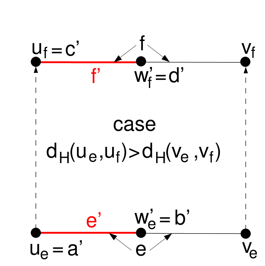
Proof of Theorem 5.3.
To prove necessity, let $C$ be the cut-set of a convex cut that partitions $V$ into $V_{1}$ and $V_{2}$ , and let $e,f\in C$ (see Figure 7). Thanks to Lemma 5.4 it suffices to find a child $\{a^{\prime},b^{\prime}\}$ of $e$ and a child $\{c^{\prime},d^{\prime}\}$ of $f$ such that $d_{H^{\prime}}(a^{\prime},c^{\prime})=d_{H^{\prime}}(b^{\prime},d^{\prime})$ . Let $w_{e}^{\prime}$ [ $w_{f}^{\prime}$ ] denote the vertex of $H^{\prime}$ that subdivides $e$ [ $f$ ]. Without loss of generality we assume $u_{e},u_{f}\in V_{1}$ and $v_{e},v_{f}\in V_{2}$ . Since $C$ is the cut-set of a convex cut, we know that $d_{H}(u_{e},u_{f})$ and $d_{H}(v_{e},v_{f})$ differ by at most one.

1.

If $d_{H}(v_{e},v_{f})=d_{H}(u_{e},u_{f})$ , let $\{a^{\prime},b^{\prime}\}=\{u_{e},w_{e}^{\prime}\}$ and $\{c^{\prime},d^{\prime}\}=\{w_{f}^{\prime},v_{f}\}$ (this is the case illustrated in Figure 7a). Then, due to the degrees of $w_{e}^{\prime}$ and $w_{f}^{\prime}$ being two, $d_{H^{\prime}}(a^{\prime},c^{\prime})=d_{H^{\prime}}(u_{e},w_{f}^{\prime})=d_{H^{\prime}}(w_{e}^{\prime},v_{f})=d_{H^{\prime}}(b^{\prime},d^{\prime})$ .
2.

If $d_{H}(u_{e},u_{f})$ and $d_{H}(v_{e},v_{f})$ differ by exactly one, we may assume without loss of generality that $d_{H}(v_{e},v_{f})=d_{H}(u_{e},u_{f})+1$ . Set $\{a^{\prime},b^{\prime}\}=\{w_{e}^{\prime},v_{e}\}$ and $\{c^{\prime},d^{\prime}\}=\{w_{f}^{\prime},v_{f}\}$ . Then, due to the degrees of $w_{e}^{\prime}$ and $w_{f}^{\prime}$ being two, $d_{H^{\prime}}(a^{\prime},c^{\prime})=d_{H^{\prime}}(w_{e}^{\prime},w_{f}^{\prime})=d_{H^{\prime}}(v_{e},v_{f})=d_{H^{\prime}}(b^{\prime},d^{\prime})$ .

Conversely, to prove sufficiency, let $C$ be the cut-set of a cut that partitions $V$ into $V_{1}$ and $V_{2}$ . We distinguish the two cases of the prerequisite.

•

Case 1 ( $e~\tau~f$ ): Then we have $d_{H}(u_{e},u_{f})=d_{H}(v_{e},v_{f})$ by definition of $\tau$ .
•

Case 2 (there exists a child $e^{\prime}$ of $e$ and a child $f^{\prime}$ of $f$ such that $e^{\prime}~\theta^{\prime}~f^{\prime}$ ): As above we assume without loss of generality that $u_{e},u_{f}\in V_{1}$ and $v_{e},v_{f}\in V_{2}$ . There are four possibilities for the positions of $e^{\prime}$ and $f^{\prime}$ within $e$ and $f$ , only two of which need to be considered due to symmetry.
1. 1.
  
  $e^{\prime}=\{u_{e},w_{e}^{\prime}\}$ and $f^{\prime}=\{w_{f}^{\prime},v_{f}\}$ . Since the degrees of $w_{e}^{\prime}$ and $w_{f}^{\prime}$ are two, and since $e^{\prime}~\theta^{\prime}~f^{\prime}$ , any shortest path from $u_{e}$ to $w_{f}^{\prime}$ runs via $u_{f}$ , and any shortest path from $w_{e}^{\prime}$ to $v_{f}$ runs via $v_{e}$ . Hence, $d_{H^{\prime}}(u_{e},u_{f})=d_{H^{\prime}}(u_{e},w_{f}^{\prime})-1=d_{H^{\prime}}(w_{e}^{\prime},v_{f})-1=d_{H^{\prime}}(v_{e},v_{f})$ .
2. 2.
  
  $e^{\prime}=\{u_{e},w_{e}^{\prime}\}$ and $f^{\prime}=\{u_{f},w_{f}^{\prime}\}$ . In this case $d_{H^{\prime}}(u_{e},u_{f})=d_{H^{\prime}}(w_{e}^{\prime},w_{f}^{\prime})=d_{H^{\prime}}(v_{e},v_{f})\pm 2$ .

To summarize Case 1 and Case 2, we always have $d_{H^{\prime}}(u_{e},u_{f})=d_{H^{\prime}}(v_{e},v_{f})\pm 2$ .

Due to $d_{H^{\prime}}(u,v)=2d_{H}(u,v)$ for all vertices $u,v$ of $H$ , we have that $d_{H}(u_{e},u_{f})=d_{H}(v_{e},v_{f})\pm 1$ for all $e=\{u_{e},v_{e}\},f=\{u_{f},v_{f}\}$ in the cut-set $C$ . Hence, any shortest path with end vertices in $V_{1}$ [ $V_{2}$ ] stays within $V_{1}$ [ $V_{2}$ ], i. e., $C$ is the cut-set of a convex cut.

6 Convex cuts of plane graphs

In this section $G=(V,E)$ is a plane graph with the restrictions formulated in Section 2. Recall that the restrictions are not essential for finding convex cuts.

We search for cut-sets of convex cuts of $G$ by brachiating from an edge $e_{0}$ of $G$ via a bounded face $F_{0}$ of $G$ , i. e., $e_{0}\in E(F_{0})$ , to an edge $e_{1}$ on $E(F_{0})\cap E(F_{1})$ for some bounded face $F_{1}$ of $G$ , and so on. Theorem 5.3 in this paper and Lemma 2 in [6] restrict and thus guide the brachiating. The latter lemma says that for the cut-set $C$ of any convex cut and any bounded face $F$ we have that $|C\cap E(F)|$ equals zero or two. Our approach to finding (cut-sets of) convex cuts through brachiating suggests the following notation.

Notation 6.1.

$C$ denotes a cut-set of a cut of $G$ and is written as a non-cyclic or cyclic (simple cycle) sequence $(e_{0},\dots,e_{|C|-1})$ . If $C$ is non-cyclic, there exist bounded faces $F_{0},\dots,F_{|C|-2}$ of $G$ such that $e_{i-1}\in E(F_{i-1})\cap E(F_{i})$ . If $C$ is cyclic there exist bounded faces $F_{0},\dots,F_{|C|-1}$ such that $e_{i-1}\in E(F_{i-1})\cap E(F_{i})$ , and indices are modulo $|C|$ .

In particular, $C\cap E(F_{\infty})=\{e_{0},e_{|C|-1}\}$ for non-cyclic $C$ and $C\cap E(F_{\infty})=\emptyset$ for cyclic $C$ .

Analogous to Section 5, $G^{\prime}=(V^{\prime},E^{\prime})$ denotes the (plane bipartite) graph that one obtains from $G$ by placing a new vertex into the interior of each edge of $G$ .

Definition 6.2 ( $e_{0}^{l}$ , $e_{0}^{r}$ , $C_{l}^{\prime}$ , $C_{r}^{\prime}$ , $C_{l}$ , $C_{r}$ , $C_{\tau}$ ).

The left [right] child of $e_{0}$ when standing on $e_{0}$ and looking into $F_{0}$ is denoted by $e_{0}^{l}$ [ $e_{0}^{r}$ ]. Furthermore, $C_{l}^{\prime}$ [ $C_{r}^{\prime}$ ] denotes the set of edges in $E^{\prime}$ that are $\theta^{\prime}$ -related to $e_{0}^{l}$ [ $e_{0}^{r}$ ]. Recall that $C_{l}^{\prime}$ and $C_{r}^{\prime}$ are cut-sets of cuts of $G^{\prime}$ . Thus, they induce cut-sets of $G$ denoted by $C_{l}$ and $C_{r}$ . Generally ”left“ and ”right“ w. r. t. an edge $e_{i}$ is from the perspective of standing on $e_{i}$ and looking into $F_{i}$ . Finally, $C_{\tau}=\{e\in E\mid e_{0}~\tau~e\}$ .

6.1 Embedding of cuts

In this section we first represent a cut of $G$ through $e_{0}$ with cut-set $C$ by a simple path or simple cycle $\gamma(C)$ in the line graph (sometimes referred to as edge graph) $L_{G}$ of $G$ . We then embed the edges of $L_{G}$ that we need for representing cuts. In particular, all $\gamma(C)$ turn into simple non-closed or closed curves.

Definition 6.3 ( $L_{G}(V^{L},E^{L})$ , cut $\gamma(C)$ ).

$L_{G}=(V^{L},E^{L})$ denotes the line graph of $G$ , i. e., $V^{L}=E$ . Using Notation 6.1, we define $\gamma(C)$ to be the path in $L_{G}$ whose edge set is

E^{L}(C)=\{\{e_{i-1},e_{i}\}\}

(4)

If $C$ is non-cyclic [cyclic], $\gamma(C)$ is a maximal simple path [simple cycle] in $L_{G}$ .

An edge $\{e,\hat{e}\}$ of $L_{G}$ can be part of $\gamma(C)$ for some $C$ only if there exists a face $F$ of $G$ such that $e,\hat{e}\in E(F)$ . To embed such an edge we proceed basically as in Section 3.2. Let $p$ and $\hat{p}$ denote the midpoints of $e$ and $\hat{e}$ , respectively. Furthermore, let $F^{r}$ denote a regular polygon with the same number of sides as $F$ , and let $\hslash:\overline{F^{r}}\mapsto\overline{F}$ be a homeomorphism (recall that $\overline{F}=F\cup E(F)$ ). We embed $\{e,\hat{e}\}$ as $\hslash(L)$ , where $L$ is the line segment between $\hslash^{-1}(p)$ and $\hslash^{-1}(\hat{p})$ . Thus, the vertices of embedded $\gamma(C)$ are all midpoints of edges of $G$ , and embedded $\gamma(C)$ is a curve that subdivides $D(G)$ into two connected components (for $D(G)$ see Definition 3.9).

6.2 Restrictive conditions for convex cuts

Any cut-set of a convex cut through $e_{0}$ must be contained in $C_{l}\cup C_{r}\cup C_{\tau}$ . This follows from Theorem 5.3, i. e., the fact that for any $e_{i}$ in $C$ it must hold that either $e_{0}~\tau~e_{i}$ or that there exists a child of $e_{0}$ and a child of $e_{i}$ that are $\theta^{\prime}$ -related.

The next lemma tells us that, on a local level, we have to deal only with $\theta^{\prime}$ and not with $\tau$ .

Lemma 6.4.

If $e_{i-1}~\tau~e_{i}$ , then $C$ cannot be the cut-set of a convex cut.

Proof.

Let $e_{i-1}=\{u_{i-1},v_{i-1}\}$ , $e_{i}=\{u_{i},v_{i}\}$ . Without loss of generality we assume that $u_{i-1}$ is on the same side of the convex cut as $u_{i}$ and that $v_{i-1}$ is on the same side of the convex cut as $v_{i}$ (see Figure 8a). Then $e_{i-1}~\tau~e_{i}$ and $e_{i-1},e_{i}\in E(F_{i-1})$ imply that any shortest path from $u_{i-1}$ to $v_{i}$ intersects any shortest path from $v_{i-1}$ to $u_{i}$ at a vertex that we denote by $w$ . Without loss of generality we may assume that $w$ is on the same side of the convex cut as $u_{i-1}$ . Due to $e_{i-1}~\tau~e_{i}$ we have $d_{G}(w,u_{i})=d_{G}(w,v_{i})$ . Thus, there exists a shortest path from $v_{i}$ via $w$ to $v_{i-1}$ that starts and ends on the side of $v_{i-1}$ , but contains the vertex $w$ , which is on the side of $u_{i-1}$ . Hence the cut cannot be convex. ∎

The observation below will lead to more restrictive conditions for convex cuts.

Observation 6.5.

The case distinction in the proof of Theorem 5.3 yields the following for plane graphs. If a child $e_{i}^{\prime}$ of $e_{i}$ is $\theta^{\prime}$ -related to a child $e_{j}^{\prime}$ of $e_{j}$ with $j\neq i$ , then exactly one of the next two cases holds.

a)

$\theta^{\prime}$ induces a one-to-one correspondence between the two children of $e_{i}$ and the two children of $e_{j}$ (see Figure 7a). If $e_{i}^{\prime}$ is the left [right] child of $e_{i}$ , then $e_{j}^{\prime}$ is the right [left] child of $e_{j}$ .
b)

The pair $e_{i}^{\prime}$ , $e_{j}^{\prime}$ is the only pair of $\theta^{\prime}$ -related children (see Figure 7b). In particular, $e_{i}^{\prime}$ and $e_{j}^{\prime}$ must be on the same side of the cut, and there exists a shortest path from the end vertex of $e_{i}$ that is also the end vertex of $e_{i}^{\prime}$ via $e_{i}$ to the end vertex of $e_{j}$ that is not an end vertex of $e_{j}^{\prime}$ . If $e_{i}^{\prime}$ is the left [right] child of $e_{i}$ , then $e_{j}^{\prime}$ is the left [right] child of $e_{j}$ .

All we know about the cut $(V_{1},V_{2})$ in the next lemma is that a pair of edges has certain children that are $\theta^{\prime}$ related. Still, $(V_{1},V_{2})$ tells us that certain convex cuts cannot exist.

Lemma 6.6.

Let $C$ be the cut-set of an embedded cut $(V_{1},V_{2})$ such that the left [right] child of $e_{i}$ is $\theta^{\prime}$ -related to a child of $e_{j}$ for some $i,j$ with $j>i$ . Then there exists no (embedded) convex cut with $e_{i}$ in its cut-set that runs right [left] of $(V_{1},V_{2})$ .

Proof.

Without loss of generality we assume that the left child of $e_{i}$ , denoted by $e^{l}_{i}$ , is $\theta^{\prime}$ -related to a child of $e_{j}$ , denoted by $e^{\prime}_{j}$ . We denote the left and right end vertex of $e_{i}$ [ $e_{j}$ ] by $u_{i}$ and $v_{i}$ [ $u_{j}$ and $v_{j}$ ], respectively. Due to Observation 6.5, one of the two following cases must hold.

1.

$d_{G^{\prime}}(u_{i},u_{j})=d_{G^{\prime}}(v_{i},v_{j})=:k$ , and $e^{\prime}_{j}$ is the right child of $e_{j}$ . This is the case illustrated in Figure 8b. The shortest path from $u_{i}$ to $v_{j}$ in $G^{\prime}$ cannot be shorter than $k+2$ , because this would entail $d_{G^{\prime}}(u_{i},v_{j})=k$ and thus $v_{j}\in W_{u_{i},v_{i}}$ , a contradiction to $e^{l}_{i}~\theta^{\prime}e^{\prime}_{j}$ . Hence, there exists a shortest path $P^{\prime}$ in $G^{\prime}$ from $u_{i}$ via $v_{i}$ to $v_{j}$ (with length $k+2$ ). A cut with $e_{i}$ in its cut-set that runs right of $(V_{1},V_{2})$ is crossed twice by $P^{\prime}$ . Hence the cut is not convex.
2.

$d_{G^{\prime}}(u_{i},u_{j})=d_{G^{\prime}}(v_{i},v_{j})+2$ , and $e^{\prime}_{j}$ is the left child of $e_{j}$ . This is the case illustrated in Figure 8c. From $e^{l}_{i}~\theta^{\prime}~e^{\prime}_{j}$ follows again that there exists a shortest path $P^{\prime}$ in $G^{\prime}$ from $u_{i}$ via $v_{i}$ to $v_{j}$ (with length $k+2$ ), and the claim follows as in the item above.

∎

We will now see that embedded $C_{l}$ and $C_{r}$ border all embedded convex cuts through $e_{0}$ .

Proposition 6.7.

1.

The embedded cut with cut-set $C_{l}$ runs on the right side of the embedded cut with cut-set $C_{r}$ (except on $C_{l}\cap C_{r}$ , where the embedded cuts touch).
2.

Any embedded convex cut runs between the embedded cut with cut-set $C_{l}$ and the embedded cut with cut-set $C_{r}$ , i. e., no part of the convex cut runs right of $C_{l}$ or left of $C_{r}$ .

Proof.

1.

We use Observation 6.5b: for any $e^{l}\in C_{l}\setminus C_{r}$ there exists a shortest path $P$ in $G^{\prime}$ from the left end vertex of $e_{0}$ via $e_{0}$ and the right end vertex of $e_{0}$ towards the right end vertex of $e^{l}$ . The assumption that parts of $C_{l}$ run on the left side of $C_{r}$ lead to a contradiction. Indeed, this would entail that there exists a shortest path $P$ as above which also crosses $C_{r}$ via an edge $e^{r}\in C_{r}$ , i. e., $P$ contains a shortest path from the left end vertex of $e_{0}^{r}$ via $e_{0}^{r}$ and the right end vertex of $e_{0}^{r}$ (which equals the right end vertex of $e_{0}$ ) and further on via the right end vertex of $e^{r}$ to the left end vertex of $e^{r}$ — a contradiction to $e^{r}\in C_{r}$ .
2.

A consequence of a special case of Lemma 6.6, i. e., the case $i=0$ .

∎

The following proposition reveals that the edges of $G$ that are not in $C_{l}\cup C_{r}$ , i. e., the edges in $C_{\tau}$ , may serve as unique sequences of stepping stones for convex cuts that move from $C_{l}$ to $C_{r}$ or vice versa.

Proposition 6.8.

Let $C=(e_{0},\dots,e_{|C|-1})$ be the cut-set of a convex cut through $e_{0}$ . Then the following holds. If $e_{i-1}\in C_{l}$ [ $e_{i-1}\in C_{r}$ ] and $e_{i}\in C_{\tau}$ , then there exists $j>i$ such that $e_{i},\dots,e_{j-1}\in C_{\tau}$ and $e_{j}\in C_{r}$ [ $e_{j}\in C_{l}$ ]. Moreover, any cut-set of a convex cut through $e_{0}$ that coincides with $C$ on $e_{0},e_{1},\dots,e_{i}$ must coincide with $C$ on $e_{0},e_{1},\dots,e_{j}$ .

Proof.

Without loss of generality we assume $e_{i-1}\in C_{l}$ .

1.

Let $e_{0}=\{u_{0},v_{0}\}$ and $e_{i}=\{u_{i},v_{i}\}$ , let $P_{u}$ [ $P_{v}$ ] be a shortest path from $u_{i}$ [ $v_{i}$ ] to $u_{0}$ in $G$ , and let $e^{u}$ [ $e^{v}$ ] be the first edge on $P_{u}$ [ $P_{v}$ ] (see Figure 9a). Then $e^{u},e^{v}\in C_{r}$ .

Without loss of generality we show that $e^{u}\in C_{r}$ . Let $w_{0}$ [ $w_{i}$ ] denote the vertex of $G^{\prime}$ that subdivides $e_{0}$ [ $e^{u}$ ]. To prove $e^{u}\in C_{r}$ , it suffices to show $\{w_{i},u_{i}\}\theta^{\prime}\{u_{0},w_{0}\}$ . Indeed, by definition of $\tau$ , we have that the length of $P_{u}$ equals $d_{G}(u_{i},v_{0})$ . Since the degrees of $w_{i}$ and $w_{0}$ are two, a shortest path from $w_{i}$ to $w_{0}$ runs via $u_{0}$ or via $v_{0}$ . In both cases the distance is $2d_{G^{\prime}}(u_{i},v_{0})$ . Thus, $\{w_{i},u_{i}\}$ is $\theta^{\prime}$ -related to $e_{0}^{r}$ , i. e., $e^{u}\in C_{r}$ .
2.

The following case distinction yields $e^{v}=e_{j}$ for some $j>i$ (see Figure 9b).
1. (a)
  
  The embedded convex cut with cut-set $C$ crosses embedded $C_{r}$ . This case cannot occur due to Lemma 6.6.
2. (b)
  
  $C$ contains $e^{u}$ . Then $\{w_{i},u_{i}\}$ is a left child of $e^{u}$ w. r. t. $C$ . Since $e_{0}^{r}$ is a right child of $e_{0}$ w. r. t. $C$ , and $e_{0}^{r}$ is $\theta^{\prime}$ -related to $\{w_{i},u_{i}\}$ (see item 2a), Observation 6.5a yields that $e_{0}^{l}$ and the right child of $e^{u}$ are $\theta^{\prime}$ -related, too. This is a contradiction to $e^{u}\in C_{r}$ (see item 1).
3. (c)
  
  The remaining case is that $C$ contains $e^{v}\in C_{r}$ , i. e., $e^{v}=e_{j}$ for some $j>i$ .
3.

It remains to show that the extension from $e_{i}$ to $e_{j}$ is unique (see Figure 9c). Indeed, let $y_{i}$ be the end vertex of $e_{j}$ that is not $v_{i}$ . The path from $u_{i}$ to $y_{i}$ via $v_{i}$ has length two and contains two edges of $C$ . Due to the cut being convex, there exists an edge $\hat{e}$ from $u_{i}$ to $y_{i}$ , i. e., the edges $e_{i}$ , $e_{j}$ and $\hat{e}$ form a triangle.

If $d_{G}(x,v_{i})<d_{G}(x,y_{i})$ , then $x$ must be on the same side of the cut as $v_{0}$ . Indeed, assume that $x$ is on the other side, i. e., the side of $u_{0}$ . Then, due to $e_{0}~\tau~e_{i}$ , i. e., $d_{G}(u_{0},u_{i})=d_{G}(u_{0},v_{i})=d_{G}(v_{0},u_{i})=d_{G}(v_{0},v_{i})$ , there exists a shortest path from $x$ via $v_{i}$ to $v_{0}$ that crosses the convex cut twice, a contradiction.

If $d_{G}(x,v_{i})\geq d_{G}(x,y_{i})$ , then $x$ must be on the same side of the convex cut as $u_{0}$ . Indeed, assume that $x$ is on the other side, i. e., the side of $v_{0}$ . Then, due to $e_{0}~\tau~e_{i}$ , there exists a path from $x$ via $y_{i}$ and $u_{0}$ to $v_{0}$ that is not longer than alternative paths of $x$ via $u_{i}$ or $v_{i}$ to $v_{0}$ . The path via $y_{i}$ thus is a shortest path from $x$ to $v_{0}$ that crosses the convex cut twice, a contradiction.

To summarize, the side of any vertex $x$ in the triangle is unique i. e., the extension from $e_{i}$ to $e_{j}$ is unique.

∎

6.3 Intersection pattern of embedded convex cuts

In Section 6.1 we represented a cut of $G$ through $e_{0}$ by an embedded simple path or simple cycle $\gamma(C)$ in the line graph $L_{G}$ of $G$ . In this section we study the intersection pattern of a pair of embedded convex cuts of $G$ through $e_{0}$ . More formally, if $C$ and $\hat{C}$ are cut-sets of convex cuts of $G$ through $e_{0}$ , we study the patterns in $\mathbb{R}^{2}$ that are formed by the curves $\gamma(C)$ and $\gamma(\hat{C})$ .

The boundary of any face $F_{L}$ of $\gamma(C)\cup\gamma(\hat{C})$ constitutes a cyclical cut of $G$ (see Figure 10). Let $v^{L}\in V^{L}$ be a vertex on the boundary of $F_{L}$ . The vertex $v^{L}$ is the midpoint of an edge $e\in C$ . In particular, one end vertex of $e$ must be contained in the interior of $F_{L}$ . Thus we have proven the following.

Lemma 6.9.

Any face of $\gamma(C)\cup\gamma(\hat{C})$ contains at least one vertex of $G$ .

Lemma 6.4 and the case of Lemma 6.6 in which $e_{i}$ and $e_{j}$ sit on the boundary of the same face of $G$ yield Proposition 6.10 (see also Figures 8b,c). It states that all embedded convex cuts through $e_{0}$ which have reached a face $F$ on the midpoint of an edge on $E(F)$ can cut through $F$ in at most two ways.

Proposition 6.10.

Let $C=(e_{0},\dots e_{|C|-1})$ be the cut-set of a convex cut of $G$ through $e_{0}$ . Then the following holds. For all $e_{i}$ in $C$ there exists $f_{i}\in E(F_{i-1})$ (possibly $e_{i}=f_{i}$ ) such that $\hat{e}_{j}\in\{e_{i}\}\cup\{f_{i}\}$ for the cut-set $\hat{C}=(e_{0},\hat{e}_{1},\dots\hat{e}_{|\hat{C}|-1})$ of any convex cut with $\hat{e}_{j-1}=e_{i-1}$ and $|\{e_{0},\hat{e}_{1},\dots\hat{e}_{j-1}\}\cap F_{i-1}|=1$ .

Definition 6.11 ( $\gamma(C)$ touches $\gamma(\hat{C})$ , $\gamma(C)$ crosses $\gamma(\hat{C})$ , overlap, crossing $M_{C,\hat{C}}$ ).

Let $C$ and $\hat{C}$ be cut-sets of cuts of $G$ through $e_{0}$ . We say that $\gamma(C)$ touches [crosses] $\gamma(\hat{C})$ on the maximal common curve $M_{C,\hat{C}}$ of $\gamma(C)$ and $\gamma(\hat{C})$ if the part of $\gamma(C)$ directly before $M_{C,\hat{C}}$ is on the same side [on the other side] of $\gamma(\hat{C})$ as the part of $\gamma(C)$ directly after $M_{C,\hat{C}}$ . The curve $M_{C,\hat{C}}$ is called an overlap of $\gamma(C)$ and $\gamma(\hat{C})$ . If $\gamma(C)$ crosses $\gamma(\hat{C})$ on $M_{C,\hat{C}}$ , we refer to $M_{C,\hat{C}}$ as the crossing of $\gamma(C)$ and $\gamma(\hat{C})$ .

For examples of touching and crossing cuts see Figure 10. The following proposition describes the intersection pattern of a pair of embedded convex cuts of $G$ through $e_{0}$ .

Proposition 6.12.

Let $C,\hat{C}$ be cut-sets of convex cuts of $G$ through $e_{0}$ . Then $\gamma(C)$ cannot touch $\gamma(\hat{C})$ , and $\gamma(C)$ and $\gamma(\hat{C})$ can have at most one crossing.

Proof.

•

Assume that $\gamma(C)$ touches $\gamma(\hat{C})$ . Let $F^{1}_{L}$ and $F^{2}_{L}$ be the faces formed by the parts of $\gamma(C)$ and $\gamma(\hat{C})$ before and after $M_{C,\hat{C}}$ , respectively (see Figure 10a). Lemma 6.9 yields that there exist vertices $v_{1}\in V\cap F^{1}_{L}$ and $v_{2}\in V\cap F^{2}_{L}$ . Any shortest path from $v_{1}$ to $v_{2}$ either crosses $\gamma(C)$ or $\gamma(\hat{C})$ twice, a contradiction to $C$ and $\hat{C}$ being cut-sets of convex cuts.
•

Assume that $\gamma(C)$ and $\gamma(\hat{C})$ have crossings $M^{1}_{C,\hat{C}}\neq M^{2}_{C,\hat{C}}$ , and that there is no crossing between $M^{1}_{C,\hat{C}}$ and $M^{2}_{C,\hat{C}}$ . Let $F^{1}_{L}$ and $F^{2}_{L}$ be the faces formed by the parts of $\gamma(C)$ and $\gamma(\hat{C})$ before $M^{1}_{C,\hat{C}}$ and after $M^{2}_{C,\hat{C}}$ , respectively (see Figure 10c). Lemma 6.9 yields that there exist vertices $v_{1}\in V\cap F^{1}_{L}$ and $v_{2}\in V\cap F^{2}_{L}$ . As in the previous item, any shortest path from $v_{1}$ to $v_{2}$ either crosses $\gamma(C)$ or $\gamma(\hat{C})$ twice, a contradiction to $C$ and $\hat{C}$ being cut-sets of convex cuts.

∎

6.4 Upper bound on number of convex cuts through $e_{0}$

To find an upper bound on the number of convex cuts of $G$ through $e_{0}$ we start by assuming that there exists at least one such cut with cut-set $\hat{C}$ . The necessary conditions for convex cuts in Section 6.2 and Proposition 6.12 impose constraints on the other candidates for convex cuts through $e_{0}$ . In particular, Proposition 6.12 implies the following. The first overlap of $\gamma(C)$ and $\gamma(\hat{C})$ is always the one that contains the midpoint of $e_{0}$ . It always exists. If there is a second overlap, and this second overlap is not a crossing, it must be the last overlap, and it must contain the midpoint of $e_{|C|-1}$ . This follows from the fact that $\gamma(C)$ and $\gamma(\hat{C})$ cannot touch. If the second overlap exists and constitutes a crossing, there may or may not be another overlap. If there exists such a third overlap, it must be the last one, and it must contain $e_{|C|-1}$ (since $\gamma(C)$ and $\gamma(\hat{C})$ cannot touch, and they cannot cross twice). Thus, we have proven the following.

Proposition 6.13 (At most three overlaps).

Let $C$ and $\hat{C}$ be cut-sets of convex cuts of $G$ through $e_{0}$ . Then $\gamma(C)$ and $\gamma(\hat{C})$ can have at most three overlaps.

Definition 6.14 (Fork and corresponding join of $\gamma(C)$ and $\gamma(\hat{C})$ , detour on $\gamma(C)$ ).

Let $C$ and $\hat{C}$ be cut-sets of cuts of $G$ through $e_{0}$ . Furthermore, let $M_{1}$ and $M_{2}$ be two consecutive overlaps of $\gamma(C)$ and $\gamma(\hat{C})$ , i. e., there is no overlap of $\gamma(C)$ and $\gamma(\hat{C})$ of $M_{1}$ and $M_{2}$ . Then the last point of $M_{1}$ and the first point of $M_{2}$ are called fork and corresponding join of $\gamma(C)$ and $\gamma(\hat{C})$ . The sub-path of $\gamma(C)$ between a fork and a corresponding join is called detour on $\gamma(C)$ around $\gamma(\hat{C})$ .

Proposition 6.15 (Unique detours).

Let $C$ , $C^{*}$ and $\hat{C}$ be cut-sets of convex cuts of $G$ through $e_{0}$ , let $p^{f}$ and $p^{j}$ be a fork and a corresponding join of $\gamma(C)$ and $\gamma(\hat{C})$ , as well as of $\gamma(C^{*})$ and $\gamma(\hat{C})$ . If $\{p^{f}\}$ is not a crossing, then the corresponding detours on $\gamma(C)$ and on $\gamma(C^{*})$ coincide.

Proof.

1.

$p^{f}$ is the midpoint of an edge of $G$ . Indeed, an edge of $\gamma(C)$ , $\gamma(C^{*})$ or $\hat{\gamma(C)}$ takes the form $\{f_{i-1},f_{i}\}$ , where $f_{i-1},f_{i}$ are edges of $G$ . Here the indices reflect the order of the corresponding cut-sets (see Notation 6.1). Moreover, there exists a face $F_{i-1}$ of $G$ with $f_{i-1},f_{i}\in F_{i-1}$ . The embedded edge $\{f_{i-1},f_{i}\}$ is a curve from the midpoint of $f_{i-1}$ through the interior of $F_{i-1}$ to the midpoint of $f_{i}$ . The embedding is such that two embedded edges that cross in a face of $G$ must cross at a single point (see Section 6.1). Thus, the condition that the join $\{p^{f}\}$ is not a crossing implies that $p^{f}$ is the midpoint of an edge of $G$ .
2.

The first edge of the detour on $\gamma(C)$ around $\gamma(\hat{C})$ from $p^{f}$ to $p^{j}$ must coincide with the first edge of the detour on $\gamma(C^{*})$ around $\gamma(\hat{C})$ . Indeed, let $e^{f}$ be the edge with midpoint $p^{f}$ . Let the successors of $e^{f}$ in the cut-sets $C$ , $C^{*}$ and $\hat{C}$ be denoted by $s$ , $s^{*}$ and $\hat{s}$ , respectively. Since $p^{f}$ and $p^{j}$ are a fork and a corresponding join of $\gamma(C)$ and $\gamma(\hat{C})$ , as well as of $\gamma(C^{*})$ and $\gamma(\hat{C})$ , the edges $\{e^{f},s\}$ , $\{e^{f},s^{*}\}$ and $\{e^{f},\hat{s}\}$ all go through the same face of $G$ . Proposition 6.10 yields that at least two of the three embedded edges must coincide. Thus, the first edge of the detour on $\gamma(C)$ around $\gamma(\hat{C})$ from $p^{f}$ and $p^{j}$ must coincide with the first edge of the detour on $\gamma(C^{*})$ around $\gamma(\hat{C})$ .
3.

Analogous to Definition 6.2, let $C^{f}_{l}$ [ $C^{f}_{r}$ ] be the set of edges of $G$ that have a child which is $\theta^{\prime}$ -related to the left [right] child of $e^{f}$ . Without loss of generality we assume that $\gamma(C)$ runs right of $\gamma(\hat{C})$ . Lemmas 6.4 and Proposition 6.10 then yield that (i) the edge in $C$ directly after $e^{f}$ , denoted by $e$ is contained in $C^{f}_{l}$ and (ii) the edge in $\hat{C}$ directly after $e^{f}$ , denoted by $\hat{e}$ , is contained in $C^{f}_{r}$ .

We assume the opposite of the claim, i. e., that $\gamma(C)$ and $\gamma(C^{*})$ fork at or behind $e$ and join at or before $p^{j}$ . Then Proposition 6.7 and Proposition 6.8 imply that one of the embedded cuts continues on $C^{f}_{l}$ , while the other one switches from $C^{f}_{l}$ to $C^{f}_{r}$ . If the switching embedded cut hits $p^{j}$ as soon as it reaches $C^{f}_{r}$ , the other embedded cut has missed $p^{j}$ , a contradiction to $p^{j}\in\gamma(C)$ and $p^{j}\in\gamma(C^{*})$ . If the switching embedded cut does not hit $p^{j}$ as soon as it reaches $C^{f}_{r}$ , the embedded cut $\gamma(\hat{C})$ has already switched from $C^{f}_{r}$ to $C^{f}_{l}$ , and must thus have hit $\gamma(C)$ or $\gamma(C^{*})$ before $p^{j}$ , a contradiction.

∎

Proposition 6.16.

An upper bound for the number of convex cuts of $G$ through $e_{0}$ is $|E|^{4}$ .

Proof.

We may assume that there exists a convex cut through $e_{0}$ with cut-set $\hat{C}$ .

1.

Number of the convex cuts $\gamma(C)$ of $G$ through $e_{0}$ that do not cross $\hat{C}$ . Proposition 6.12 yields that there can be at most one fork and corresponding join of $\gamma(\hat{C})$ and $\gamma(C)$ . The number of $\gamma(C)$ is thus bounded by the number of detours around $\gamma(\hat{C})$ . Proposition 6.15 yields that the number of detours cannot surmount the number of forks of $\gamma(\hat{C})$ and $\gamma(C)$ times the number of corresponding joins of $\gamma(\hat{C})$ and $\gamma(C)$ , i. e., at most $|E|(|E|-1)/2$ .
2.

Number of the convex cuts $\gamma(C)$ of $G$ through $e_{0}$ that cross $\hat{C}$ . We first select a sub-path $M_{\hat{C}}$ of $\gamma(\hat{C})$ and determine the number of $\gamma(C)$ that cross $\gamma(\hat{C})$ on $M_{\hat{C}}$ . Let $\gamma(C)$ be such a path. $\gamma(C)$ joins $\gamma(\hat{C})$ at the first point of $M_{\hat{C}}$ , denoted by $p^{j}$ . Using Proposition 6.12 we get that $\gamma(C)$ coincides with $\gamma(\hat{C})$ between $e_{0}$ and the last point of $M_{\hat{C}}$ , with the exception of at most one detour before $M_{\hat{C}}$ . We already know that $p^{j}$ is the join of a detour. Using Proposition 6.15 we get that the number of detours before $M_{\hat{C}}$ is less than $|E|$ . The same holds for the number of detours behind $M_{\hat{C}}$ . Thus, the number of $\gamma(C)$ that cross $\gamma(\hat{C})$ on $M_{\hat{C}}$ is less than $|E|^{2}$ . The number of non-empty sub-paths $M_{\hat{C}}$ of $\gamma(\hat{C})$ , in turn, amounts to $|E|(|E|-1)/2$ . Hence, the number of $\gamma(C)$ that cross $\gamma(\hat{C})$ is less than $(|E|^{4}-|E|^{3})/2$ .

The total number of convex cuts of $G$ through $e_{0}$ thus cannot surmount $|E|^{4}$ . ∎

6.5 Algorithm for finding all convex cuts

We search for convex cuts of $G$ using a subgraph $S$ of $L_{G}=(V^{L},E^{L})$ (for $L_{G}$ see Definition 6.3).

Definition 6.17 (Search graph $S=(V_{S},E_{S})$ ).

We set
$E_{S}=\{\{e,f\}\in E^{L}\mid\{e,f\}\in E(F)\mbox{~for some face $F$ of $G$ and $e^{\prime}~\theta^{\prime}~f^{\prime}$ for children $e^{\prime}$ of $e$ and $f^{\prime}$ of $f$}\}$ . The search graph $S$ is the subgraph of $L_{G}$ that is induced by $E_{S}$ .

Definition 6.18.

We say that $v_{S},w_{S}\in V_{S}$ are compatible, if (i) a child of $v_{S}$ is $\theta^{\prime}$ related to a child of $w_{S}$ or (ii) $v_{S}~\tau~w_{S}$ .

Theorem 5.3 and Proposition 6.4 yield the following characterization of convex cuts in terms of the search graph $S$ .

Lemma 6.19.

Let $C$ be a non-cyclic [cyclic] cut-set of a cut of $G$ through $e_{0}$ . Then the cut is convex if and only if $\gamma(C)$ is a maximal path [cycle] in $S$ such that any pair of vertices $v_{S}\neq w_{S}$ on the path [cycle] is compatible.

If the cut-set $C$ of a cut of $G$ is non-cyclic, we have $C\cap E(F_{\infty})=\{e_{0},e_{|C|-1}\}$ , and if $C$ is cyclic, we have $C\cap E(F_{\infty})=\emptyset$ .

The two matrices defined next will allow us to check in constant time whether two vertices of $S$ are compatible. We build a $|E|\times|E|$ matrix $A_{\tau}$ with boolean entries such that $A_{\tau}(i,j)$ is true if and only if edge $i$ is $\tau$ -related to edge $j$ . Likewise, we build a $(2|E|)\times 2(|E|)$ matrix $A_{\theta^{\prime}}$ with boolean entries such that $A_{\theta^{\prime}}(i,j)$ is true if and only if edge $i$ in $G^{\prime}$ is $\theta^{\prime}$ -related to edge $j$ in $G^{\prime}$ .

Our algorithm for finding (the cut-sets of) all convex cuts of $G$ consists of two steps: find the non-cyclic cut-sets starting at each $e_{0}\in E(F_{\infty})$ and then find the cyclic ones starting at each $e_{0}\notin E(F_{\infty})$ . In both steps we carry along and extend paths $(e_{0},\dots,e_{k})$ of $S$ as long as all its vertices are pairwise compatible. If $e_{0}\in E(F_{\infty})$ , there exists only one bounded face $F_{0}$ whose boundary contains $e_{0}$ and the candidates for $e_{1}$ . If $e_{0}\notin E(F_{\infty})$ , there exist two such faces, and we arbitrarily declare one of them to be $F_{0}$ .

If, after starting at $e_{0}\in E(F_{\infty})$ , a path we carry along has reached $E(F_{\infty})$ again, we have found a non-cyclic oriented cut-set of a convex cut and store it (recall that the vertices of the path are pairwise compatible). When we are done with $e_{0}$ , i. e., when none of the paths that we carry along can be extended, we insert $e_{0}$ into a tabu list for further searches (we have already found all convex cuts through $e_{0}$ ). The tabu list ensures that we do not end up with two copies of a convex cut, i. e., one for each orientation. Any non-cyclic cut-set of a convex cut is found by our algorithm since it carries along one orientation of any pairwise compatible non-cyclic cut-set starting at $e_{0}$ .

If, after starting at $e_{0}\notin E(F_{\infty})$ , a path we carry along has reached $e_{0}$ again, we have found a cyclic cut-set of a convex cut and store it. Conversely, any cyclic cut-set of a convex cut is found by our algorithm since it carries along one orientation of any pairwise compatible cyclic cut-set starting at $e_{0}$ . Here, the orientation is given by the choice of $F_{0}$ (see above). Again, we insert $e_{0}$ into a tabu list.

Algorithm 2 Finding the cut-sets

C

of all convex cuts of a plane graph

G

1: Build the search graph and the matrices

A_{\tau}

and

A_{\theta^{\prime}}

2: For any start vertex

e_{0}

S

with

e_{0}\in E(F_{\infty})

perform a breadth-first-traversal (BFT) starting at

e_{0}

. The first path carried along is

(e_{0})

. For any new vertex

v_{S}

S

that is visited by the BFT and that is not in the tabu list, and for any path and cycle carried along, use the matrices

A_{\tau}

and

A_{\theta^{\prime}}

to check whether

v_{s}

is compatible with the path or the cycle. Whenever

E(F_{\infty})

is reached, store

C

and put

e_{0}

into the tabu list.

3: For any

e_{0}\notin E(F_{\infty})

declare one of the two bounded faces with

e_{0}

on their boundaries to be

F_{0}

. Proceed as in the case

e_{0}\in E(F_{\infty})

, except that (i) when at

e_{0}

, the BFT is restricted such that only edges in

E(F_{0})

are found and (ii)

C

is stored only if

e_{0}

is reached. Finally, put

e_{0}

into the tabu list.

Theorem 6.20.

Algorithm 2 finds all convex cuts of $G=(V,E)$ using $\mathcal{O}(|V|^{7})$ time and $\mathcal{O}(|V|^{5})$ space.

Proof.

Algorithm 2 is correct due to Lemma 6.19 and the fact that we find any maximal path and cycle in $S$ with pairwise compatible vertices exactly once.

To build the matrix $A_{\tau}$ , we iterate over all vertices $v_{S}$ of $S$ and identify all vertices of $S$ that are $\tau$ -related to $v_{S}$ . For a given vertex $v_{S}$ this can be done in $\mathcal{O}(|V|)$ time. Indeed, if $e=\{u,v\}$ is the edge in $G$ that equals $v_{S}$ , we can compute the distances of any $w\in V$ to $u$ and $v$ in $\mathcal{O}(|V|)$ , e. g., by using BFT. For any $f\in E$ we can then determine in constant time whether $e~\tau~f$ .

To build the matrix $A_{\theta^{\prime}}$ , we proceed as above, except that we use $G^{\prime}$ instead of $G$ . The running time for computing $A_{\tau}$ and $A_{\theta^{\prime}}$ is $\mathcal{O}(|E|^{2})$ , and $A_{\tau}$ and $A_{\theta^{\prime}}$ take $\mathcal{O}(|E|^{2})$ space.

Any time the BFT reaches a new vertex $v_{S}$ of $S$ , the paths and cycles carried along need to be checked for compatibility with $v_{s}$ . Using the matrices $A_{\tau}$ and $A_{\theta^{\prime}}$ , this takes $\mathcal{O}(|E|)$ time per path. According to Proposition 6.16 the number of convex cuts of $G$ through a starting edge $e_{0}$ is bounded by $|E|^{4}$ . This is also the maximal number of paths that we carry along and that need to be checked. Hence, processing $v_{S}$ takes time $\mathcal{O}(|E|)^{5}$ . Finding all convex cuts through a starting edge can then be done in $\mathcal{O}(|E|^{6})$ time and, since there are $|E|$ starting edges, total running time is $\mathcal{O}(|E|^{7})$ . Storing the $|E|^{4}$ paths and cycles takes $\mathcal{O}(|E|^{5})$ space.

The time and space requirements of (constructing) the search graphs and the tabu lists are below the time and space requirements specified so far. The claim now follows from $\mathcal{O}(|E|)=\mathcal{O}(|V|)$ which, in turn, is a consequence of $G$ being plane. ∎

7 Conclusions

We have presented an algorithm for finding all convex cuts of a plane graph in polynomial time. To the best of our knowledge, it is the first polynomial-time algorithm for this task. We have also presented an algorithm that computes all convex cuts of a not necessarily plane but bipartite graph in cubic time.

Both algorithms are based on binary, symmetric, but generally not transitive relations on edges. In the case of a plane graph $G$ we employed two relations: (i) the Djoković relation on the edges of a subdivision of $G$ and (ii) another relation on the edges of $G$ . In case of a bipartite graph it was sufficient to employ the Djoković relation on the graph’s edges.

To prove that the number of convex cuts of a plane graph is not exponential, we employed results on the intersection pattern of convex cuts that are based on a specific embedding of the cuts. Thus, a connection to the first part of the paper arises, where we defined a sub-class of plane graphs via the intersection patterns of certain embedded cuts (which all turned out to be convex). In particular, the transition from the sub-class to general plane graphs is reflected by a generalization of the intersection patterns of convex cuts from arrangements of pseudolines to patterns where forks and joins of convex cuts are possible.

The characterization of convex cuts of general graphs, as given by Theorem 5.3, was instrumental in finding all convex cuts of a bipartite or a plane graph in polynomial time. We reckon that this new characterization of convex cuts of general graphs also helps when devising polynomial-time algorithms for finding convex cuts in graphs from other classes.

Acknowledgments.

We thank our colleagues Andreas Gemsa, Peter Sanders, and Christian Schulz for helpful discussions on the topic.

References

[1] D. Artigas, S. Dantas, M. Dourado, and J. Szwarcfiter. Partitioning a graph into convex sets. Discrete Mathematics, 311(17):1968 – 1977, 2011.
[2] P. Balister, S. Gerke, G. Gutin, A. Johnstone, J. Reddington, E. Scott, A. Soleimanfallah, and A. Yeo. Algorithms for generating convex sets in acyclic digraphs. Journal of Discrete Algorithms, 7(4):509 – 518, 2009.
[3] C. Bichot and P. Siarry. Graph Partitioning. Wiley, 2011.
[4] A. Björner, M. Las Vergnas , B. Sturmfels, N. White, and G. Ziegler. Oriented Matroids. Encyclopedia of Mathematics and its Applications, 46. Cambridge University Press, second edition, 1999.
[5] A. Buluç, H. Meyerhenke, I. Safro, P. Sanders, and C. Schulz. Recent advances in graph partitioning. eprint arXiv:1311.3144, http://arxiv.org/abs/1311.3144, Dec 2013.
[6] V. Chepoi, M. Deza, and V. Grishukhin. Clin d’œil on $L_{1}$ -embeddable planar graphs. Discrete Applied Mathematics, 80:3–19, 1997.
[7] D. Delling, A. V. Goldberg, I. Razenshteyn, and R. F. F. Werneck. Graph partitioning with natural cuts. In Proc. 25th IEEE Intl. Parallel and Distributed Processing Symposium (IPDPS’11), pages 1135–1146, 2011.
[8] R. Diestel. Graph Theory. Graduate texts in mathematics. Springer, 2006.
[9] D. Djoković. Distance-Preserving Subgraphs of Hypercubes. Journal of Combinatorial Theory B, 14:263–267, 1973.
[10] M. Dourado, F. Protti, D. Rautenbach, and J. Szwarcfiter. On the convexity number of graphs. Graphs and Combinatorics, 28:333–345, 2012.
[11] D. Eppstein. Cubic Partial Cubes from Simplicial Arrangements. The electronic journal of combinatorics, 13: $\#$ R79, 2006.
[12] R. Glantz and H. Meyerhenke. Finding all convex cuts of a plane graph in cubic time. In Proc. 8th International Conference on Algorithms and Complexity (CIAC’13), pages 246–263, 2013.
[13] H. Meyerhenke, B. Monien, and T. Sauerwald. A new diffusion-based multilevel algorithm for computing graph partitions. Journal of Parallel and Distributed Computing, 69(9):750–761, 2009. Best Paper Awards and Panel Summary: IPDPS 2008.
[14] S. Ovchinnikov. Partial cubes: Structures, characterizations, and constructions. Discrete Mathematics, 308:5597–5621, 2008.
[15] I. Peterin. A characterization of planar partial cubes. Discrete Mathematics, 308(24):6596–6600, 2008.
[16] C. Thomassen. The Jordan-Schönflies Theorem and the Classification of Surfaces. The American Mathematical Monthly, 99:116–130, 1992.
[17] E. Wilkeit. Isometric Embeddings in Hamming Graphs. Journal of Combinatorial Theory B, 14:179–197, 1990.

Finding all convex cuts of a plane graph in polynomial time

Abstract

1 Introduction

1.1 Related work

1.2 Paper outline and contribution

2 Preliminaries

3 Partial cubes from embedding alternating paths

3.1 Alternating paths

Definition 3.1 (Opposite edges, left, right, unique opposite edge).

Definition 3.2 (Alternating path graph A⁡(G)=(VA,EA)A(G)=(V_{A},E_{A})).

Definition 3.3 ((Multiset 𝒫⁡(G)\mathcal{P}(G) of) alternating paths in A⁡(G)A(G)).

3.2 Embedding of alternating paths

Proposition 3.4.

Proof.

Definition 3.5 (Arrangement of alternating paths).

Proposition 3.6.

Proof.

Definition 3.7 (Well-arranged graph).

3.3 Partial cubes from well-arranged graphs

Notation 3.8.

Definition 3.9 (Domain D⁡(G)D(G) of GG, facet of ℰ⁡(G)\mathcal{E}(G), adjacent facets).

Definition 3.10 (DEAP graph Gℰ{G}_{\mathcal{E}} of GG).

Definition 3.11 (Primal, intermediate and star vertex of Gℰ{G}_{\mathcal{E}}).

Definition 3.12.

Theorem 3.13.

Proof.

Corollary 3.14.

3.4 Convex Cuts from Alternating Paths

Definition 3.15 (Subgraph Gℰ~\widetilde{{G}_{\mathcal{E}}} of Gℰ{G}_{\mathcal{E}}).

Lemma 3.16.

Proof.

Proposition 3.17.

Proof.

4 Convex cuts of bipartite graphs

Lemma 4.1.

Proof.

Theorem 4.2.

Proof.

5 Convex cuts of general graphs

Definition 5.1 (Relation τ\tau).

Lemma 5.2.

Theorem 5.3.

Lemma 5.4.

Proof.

6 Convex cuts of plane graphs

Notation 6.1.

Definition 6.2 (e0le_{0}^{l}, e0re_{0}^{r}, Cl′C_{l}^{\prime}, Cr′C_{r}^{\prime}, ClC_{l}, CrC_{r}, CτC_{\tau}).

6.1 Embedding of cuts

Definition 6.3 (LG​(VL,EL)L_{G}(V^{L},E^{L}), cut γ⁡(C)\gamma(C)).

6.2 Restrictive conditions for convex cuts

Lemma 6.4.

Proof.

Observation 6.5.

Lemma 6.6.

Proof.

Proposition 6.7.

Proof.

Proposition 6.8.

Proof.

6.3 Intersection pattern of embedded convex cuts

Lemma 6.9.

Proposition 6.10.

Definition 6.11 (γ⁡(C)\gamma(C) touches γ⁡(C^)\gamma(\hat{C}), γ⁡(C)\gamma(C) crosses γ⁡(C^)\gamma(\hat{C}), overlap, crossing MC,C^M_{C,\hat{C}}).

Proposition 6.12.

Proof.

6.4 Upper bound on number of convex cuts through e0e_{0}

Proposition 6.13 (At most three overlaps).

Definition 6.14 (Fork and corresponding join of γ⁡(C)\gamma(C) and γ⁡(C^)\gamma(\hat{C}), detour on γ⁡(C)\gamma(C)).

Proposition 6.15 (Unique detours).

Proof.

Proposition 6.16.

Proof.

6.5 Algorithm for finding all convex cuts

Definition 6.17 (Search graph S=(VS,ES)S=(V_{S},E_{S})).

Definition 6.18.

Lemma 6.19.

Theorem 6.20.

Proof.

7 Conclusions

Acknowledgments.

Definition 3.2 (Alternating path graph $A(G)=(V_{A},E_{A})$ ).

Definition 3.3 ((Multiset $\mathcal{P}(G)$ of) alternating paths in $A(G)$ ).

Definition 3.9 (Domain $D(G)$ of $G$ , facet of $\mathcal{E}(G)$ , adjacent facets).

Definition 3.10 (DEAP graph ${G}_{\mathcal{E}}$ of $G$ ).

Definition 3.11 (Primal, intermediate and star vertex of ${G}_{\mathcal{E}}$ ).

Definition 3.15 (Subgraph $\widetilde{{G}_{\mathcal{E}}}$ of ${G}_{\mathcal{E}}$ ).

Definition 5.1 (Relation $\tau$ ).

Definition 6.2 ( $e_{0}^{l}$ , $e_{0}^{r}$ , $C_{l}^{\prime}$ , $C_{r}^{\prime}$ , $C_{l}$ , $C_{r}$ , $C_{\tau}$ ).

Definition 6.3 ( $L_{G}(V^{L},E^{L})$ , cut $\gamma(C)$ ).

Definition 6.11 ( $\gamma(C)$ touches $\gamma(\hat{C})$ , $\gamma(C)$ crosses $\gamma(\hat{C})$ , overlap, crossing $M_{C,\hat{C}}$ ).

6.4 Upper bound on number of convex cuts through $e_{0}$

Definition 6.14 (Fork and corresponding join of $\gamma(C)$ and $\gamma(\hat{C})$ , detour on $\gamma(C)$ ).

Definition 6.17 (Search graph $S=(V_{S},E_{S})$ ).