Additive inverse regression models with convolution-type operators

Thimo Hildebrandt Nicolai Bissantz Holger Dette Affiliation: Ruhr-Universität Bochum Affiliation: Fakultät für Mathematik Affiliation: 44780 Bochum Affiliation: Germany Affiliation: email: thimo.hildebrandt@ruhr-uni-bochum.de Email: nicolai.bissantz@ruhr-uni-bochum.de Email: holger.dette@ruhr-uni-bochum.de Affiliation: FAX: +49 2 34 32 14 559

Abstract

a
In a recent paper Birke and Bissantz, (2008) considered the problem of nonparametric estimation in inverse regression models with convolution-type operators. For multivariate predictors nonparametric methods suffer from the curse of dimensionality and we consider inverse regression models with the additional qualitative assumption of additivity. In these models several additive estimators are studied. In particular, we investigate estimators under the random design assumption which are applicable when observations are not available on a grid. Finally, we compare this estimator with the marginal integration and the non-additive estimator by means of a simulation study. It is demonstrated that the new method yields a substantial improvement of the currently available procedures.

Keywords: Inverse regression, Additive models, Convolution-type operators

Mathematical subject codes: primary, 62G08; secondary, 62G15, 62G20

1 Introduction

Inverse models have numerous applications in such important fields as biology, astronomy, economy or physics, where they have been intensively studied in a deterministic framework [Engl et al., (1996), Saitoh, (1997)]. Recently inverse problems have also found considerable interest in the statistical literature. These investigations reflect the demand in applications to quantify the uncertainty of estimates or to validate the model assumptions by the construction of statistical confidence regions or hypotheses tests, respectively [see Mair and Ruymgaart, (1996), Kaipio and Somersalo, (2010), Bissantz et al., 2007b (), Cavalier, (2008), Bertero et al., (2009), Bertero et al., (2009) or Birke et al., (2010) among others]. In this paper we are interested in the convolution type inverse regression model

(1.1)

\displaystyle Y

\displaystyle=

\displaystyle g(\textbf{z})+\varepsilon=\int_{\mathbb{R}^{d}}\psi(\textbf{z}-\textbf{t})\theta(\textbf{t})d(\textbf{t})+\varepsilon

with a known function $\psi:\mathbb{R}^{d}\rightarrow\mathbb{R}$ [e.g. Adorf, (1995)] and a centered noise term $\varepsilon$ . The goal of the experiment is to recover the signal $\theta:\mathbb{R}^{d}\rightarrow\mathbb{R}$ from data $(\textbf{z}_{\textbf{1}},Y_{\textbf{1}}),\ldots,(\textbf{z}_{\textbf{n}},Y_{\textbf{n}})$ which is closely related to deconvolution [e.g. Stefanski and Carroll, (1990) and Fan, (1991)]. Models of the type (1.1) have important applications in the recovery of images from astronomical telescopes or fluorescence microscopes in biology. Therefore statistical inference for the problem of estimating the signal $\theta$ in model (1.1) has become an important field of research in recent years, where the main focus is on a one dimensional predictor. Bayesian methods have been investigated in Bertero et al., (2009) and Kaipio and Somersalo, (2010) and nonparametric methods have been proposed by Mair and Ruymgaart, (1996), Cavalier, (2008) and Bissantz et al., 2007b () among others.

In the present paper we investigate convergence properties of Fourier-based estimators for the function $\theta$ with the following purposes. Firstly, our research is motivated by the fact that deconvolution problems often arise with a multivariate predictor such as location and time. For this situation Birke and Bissantz, (2008) proposed a nonparametric estimate of the signal $\theta$ and derived its asymptotic properties under rather strong assumptions. We will discuss the nonparametric estimation problem for the signal $\theta$ under substantially weaker assumptions. Secondly, because nonparametric estimation usually suffers from the curse of dimensionality improved estimators incorporating qualitative assumptions such as additivity or multiplicity are investigated under the fixed and the random design assumption. While additive estimation has been intensively discussed for direct problems from different perspectives [see Linton and Nielsen, 1995b (), Mammen et al., (1999), Carroll et al., (2002), Hengartner and Sperlich, (2005), Nielsen and Sperlich, (2005), Doksum and Koo, (2000), Horowitz and Lee, (2005), Lee et al., (2010), Dette and Scheder, (2011)] - to our best knowledge - only one additive estimator is available for indirect inverse regression models so far where it is assumed that the observations are available on a grid [see Birke et al., (2012)]. In this paper we are particularly interested in two alternative additive estimators. The first one is applicable if observations are available on a grid but has a substantially simpler structure than the method proposed by the last-named authors, which makes it very attractive for practitioners. Moreover, it also yields substantially more precise estimates than the method of Birke et al., (2012). The second estimator is additionally applicable in the case of random predictors.
Thirdly, we will also investigate the case of correlated errors in the inverse regression model (1.1), which has - to our best knowledge - not been considered so far although it appears frequently in applications. Finally, we do not assume that the kernel $\psi$ is periodic, which is a common assertion in inverse regression models with convolution operator [see e.g. Cavalier and Tsybakov, (2002)]. Note that for many problems such as the reconstruction of astronomical and biological images from telescopic and microscopic imaging devices this assumption is unrealistic.

The remaining part of this paper is organized as follows. In Section 2 we introduce the necessary notation, different types of designs and estimators studied in this paper. Section 3 is devoted to the asymptotic properties of the estimators and we establish asymptotic normality of all considered (appropriately standardized) statistics. In Section 4 we explain how the results are changing for dependent data while Section 5 presents a small simulation study of the finite sample properties of the proposed methods. In particular we compare the new additive estimator with the currently available methods and demonstrate its superiority by a factor 6-8 with respect to mean squared error. Finally all details regarding the proofs of our asymptotic results can be found in Section 6.

2 Preliminaries

Recall the definition of model (1.1) where we assume that the moments $E[\varepsilon^{k}]$ exist for all $k\in\mathbb{N}$ such that $E[\varepsilon]=0$ and $\sigma^{2}=E[\varepsilon^{2}]>0$ . For the sake of transparency we assume at this point that the errors corresponding to different predictors are independent - for the more general case of an error process with an MA( $q$ )-structure, see Section 4. We will investigate various estimators under two assumptions regarding the explanatory variables z.

(FD)

Under the fixed design assumption we assume that observations are available on a grid of increasing size. More precisely we consider a sequence $a_{n}\to 0$ as $n\to\infty$ and assume that at each location $\textbf{z}_{\textbf{k}}=\frac{\textbf{k}}{na_{n}}\in\mathbb{R}^{d}$ with $\textbf{k}=(k_{1},...,k_{d})\in\{-n,...,n\}^{d}$ a pair of observations $(\textbf{z}_{\textbf{k}},Y_{\textbf{k}})$ is available in the model

(2.1)

\displaystyle Y_{\textbf{k}}=g(\textbf{z}_{\textbf{k}})+\varepsilon_{\textbf{k}}=\int_{\mathbb{R}^{d}}\psi(\textbf{z}_{\textbf{k}}-\textbf{t})\theta(\textbf{t})d\textbf{t}+\varepsilon_{\textbf{k}},

where $\{\varepsilon_{\textbf{k}}\>|\>\textbf{k}\in\{-n,...,n\}^{d}\}$ are independent and identically distributed random variables. Under this assumption the sample size is $N=(2n+1)^{d}$ . Note that formally the random variables $\{Y_{\textbf{k}}\>|\>\textbf{k}\in\{-n,...,n\}^{d}\}$ form a triangular array, but we do not reflect this dependence in the notation. In other words we will use the notation $Y_{\textbf{k}},\textbf{z}_{\textbf{k}},\varepsilon_{\textbf{k}}$ instead of $Y_{\textbf{k},n},\textbf{z}_{\textbf{k},n},\varepsilon_{\textbf{k},n}$ throughout this paper.

(RD)

Under the random design assumption we assume that the explanatory variables are realizations of independent, identically distributed random variables $\textbf{X}_{1,n},...,\textbf{X}_{n,n}$ with a density $f_{n}$ . Again we will not reflect the triangular structure in the notation and use $Y_{k},\textbf{X}_{k},\varepsilon_{k}$ and $f$ instead of $Y_{k,n},\textbf{X}_{k,n},\varepsilon_{k,n}$ and $f_{n}$ , respectively, that is

(2.2)

\displaystyle Y_{k}=g(\textbf{X}_{k})+\varepsilon_{k}=\int_{\mathbb{R}^{d}}\psi(\textbf{X}_{k}-\textbf{t})\theta(\textbf{t})d\textbf{t}+\varepsilon_{k};\quad k\in\{1,...,n\},

where $\varepsilon_{1},...,\varepsilon_{n}$ are independent identically distributed random variables. Under this assumption the sample size is $N=n$ .

We will use different estimators in both scenarios (2.1) and (2.2). Note that assumption (FD) assumes that observations are available on a complete $d$ -dimensional grid of length ${1\over na_{n}}$ . In this case an estimator of the signal $\theta$ has also been studied by Birke and Bissantz, (2008). The estimator in model (2.2) under assumption (RD), which is proposed in the following section, could also be used if not all observations are available on the grid.

2.1 Unrestricted estimation for random design

Fourier-based estimators have been considered by numerous authors in the univariate case (e.g. Diggle and Hall, (1993), Mair and Ruymgaart, (1996), Cavalier and Tsybakov, (2002) and Bissantz et al., 2007a ()) and its generalization to the multivariate case considered in the models (2.1) and (2.2) is straightforward. For model (2.1) a Fourier-based estimator is given by

(2.3)

\displaystyle\hat{\theta}^{FD}(\textbf{x}^{*})=\frac{1}{(2\pi)^{d}}\int_{\mathbb{R}^{d}}e^{-i\langle\textbf{w},\textbf{x}^{*}\rangle}\Phi_{K}(h\textbf{w})\frac{\hat{\Phi}^{FD}(\textbf{w})}{\Phi_{\psi}(\textbf{w})}d\textbf{w},

where

\displaystyle\hat{\Phi}^{FD}(\textbf{w})

\displaystyle=

\displaystyle\frac{1}{n^{d}a_{n}^{d}}\sum_{\textbf{k}\in\{-n,...,n\}^{d}}Y_{\textbf{k}}e^{i\langle\textbf{w},\textbf{z}_{k}\rangle}.

denotes the empirical Fourier transform, $\langle\textbf{v},\textbf{w}\rangle$ is the standard inner product of the vectors $\textbf{v},\textbf{w}\in\mathbb{R}^{d}$ and $\Phi_{K}$ and $\Phi_{\psi}$ denote the Fourier transform of a kernel function $K$ and the convolution function $\psi$ (which is assumed to be known), respectively. Moreover, in (2.3) the quantity $h$ is a bandwidth converging to $0$ with increasing sample size. Birke et al., (2012) used this estimator to construct improved estimators under the qualitative assumption of additivity in the case of a fixed design. In Section 2.2 we will propose an alternative additive estimator in the case of fixed design, which provides a notable improvement of the estimator proposed by the last named authors.
For a random design we will use the same Fourier-based estimator as defined in (2.3), where the empirical Fourier transform $\hat{\Phi}^{FD}(w)$ in (2.3) is replaced by

(2.4)

\displaystyle\hat{\Phi}^{RD}(\textbf{w})

\displaystyle=

\displaystyle\frac{1}{n}\sum_{k=1}^{n}e^{i\langle\textbf{w},\textbf{X}_{k}\rangle}\frac{Y_{k}}{\max\{f(\textbf{X}_{k}),f(\frac{1}{\textbf{a}_{\textbf{n}}})\}},

$1/\textbf{a}_{n}=(1/a_{n},...,1/a_{n})\in\mathbb{R}^{d}$ and $a_{n}$ is again a sequence converging to $0$ with increasing sample size. The resulting estimator will be denoted by $\hat{\theta}^{RD}(\textbf{x}^{*})$ . In (2.4) $f$ denotes the density of $\textbf{X}_{1}$ and we take the maximum of $f(\textbf{X}_{k})$ and $f(\frac{1}{\textbf{a}_{\textbf{n}}})$ to ensure that the variance of $\hat{\theta}^{RD}(\textbf{x}^{*})$ is bounded. We also note that the estimator $\hat{\theta}^{RD}$ admits the representation

(2.5)

\displaystyle\hat{\theta}^{RD}(\textbf{x}^{*})

\displaystyle=

\displaystyle\sum_{k=1}^{n}Y_{k}w_{n}(\textbf{x}^{*},\textbf{X}_{k}),

where the weights are given by

(2.6)

\displaystyle w_{n}(\textbf{x}^{*},\textbf{X}_{k})

\displaystyle=

\displaystyle\frac{1}{n\max\{f(\textbf{X}_{k}),f(\frac{1}{{\bf a_{n}}})\}(2\pi)^{d}}\int_{\mathbb{R}^{d}}e^{-i\langle\textbf{w},\textbf{x}^{*}-\textbf{X}_{k}\rangle}\frac{\Phi_{K}(h\textbf{w})}{\Phi_{\psi}(\textbf{w})}d\textbf{w}.

Remark 2.1.

Note that we use the same bandwidth for all components of the predictor. This assumption is made for the sake of a transparent presentation of the results. In applications the components of the vector x represent different physical quantities such that different bandwidths have to be used. All results presented in this paper can be modified to this case with an additional amount of notation.

2.2 Estimation of additive inverse regression models

It is well known that in practical applications nonparametric methods as introduced in Section 2.1 suffer from the curse of dimensionality and therefore do not yield precise estimates of the signal $\theta$ with a multivariate predictor. A common approach in nonparametric statistics to deal with this problem is to postulate an additive structure of the signal $\theta$ , that is

(2.7)

\displaystyle\theta(\textbf{x}^{*})=\theta^{add}(\textbf{x}^{*}):=\theta_{0}^{add}+\sum_{j=1}^{m}\theta_{I_{j}}^{add}(\textbf{x}_{I_{j}}^{*})

[see Hastie and Tibishirani, (2008)]. Here $\{I_{1},...,I_{m}\}$ denotes a partition of the set $\{1,...,d\}$ with cardinalities $|I_{j}|=d_{j}$ and $\textbf{x}_{I_{j}}^{*}$ is the vector which includes all components of the vector $\bf{x}^{*}$ with corresponding indices $i\in I_{j}$ . Furthermore $\theta_{0}^{add}$ is a constant and $\theta_{I_{j}}^{add}:\mathbb{R}^{d_{j}}\rightarrow\mathbb{R}$ denote functions normalized such that

\int\theta_{I_{j}}^{add}(\textbf{x})d(\textbf{x})=0\quad(j=1,...,m).

Note that the completely additive case is obtained for the choice $m=d$ , that is $d_{1}=...=d_{d}=1$ . In the case of direct regression models several estimation techniques such as marginal integration [see Linton and Nielsen, 1995b (), Carroll et al., (2002), Hengartner and Sperlich, (2005)], backfitting [Mammen et al., (1999), Nielsen and Sperlich, (2005)] have been proposed in the literature. Recently the estimation problem of an additive (direct) regression model has also found considerable interest in the context of quantile regression [see Doksum and Koo, (2000), De Gooijer and Zerom, (2003), Horowitz and Lee, (2005), Lee et al., (2010), Dette and Scheder, (2011) among others] but - to our best knowledge - only one estimator has been proposed for additive inverse regression models under the assumption that observations are available on a grid [see Birke et al., (2012)]. For this situation we will propose an alternative estimator in the following section, which yields an improvement by a factor 6-10 with respect to mean squared error (see our numerical results in Section 5).

To construct an estimator in the additive inverse regression model (2.7) with random design we apply the marginal integration method introduced in Linton and Nielsen, 1995a () to the statistic defined in (2.5). To this end we consider weighting functions $Q_{I_{1}},...,Q_{I_{m}},Q_{I_{j}}:\mathbb{R}^{d_{j}}\rightarrow\mathbb{R}$ and define

	$\displaystyle Q(\textbf{x}^{*})$	$\displaystyle=$	$\displaystyle Q_{I_{1}}(\textbf{x}_{I_{1}}^{})...Q_{I_{m}}(\textbf{x}_{I_{m}}^{})$
(2.8)		$\displaystyle Q_{I_{j}^{c}}(\textbf{x}_{I_{j}^{c}}^{*})$	$\displaystyle=$	$\displaystyle Q_{I_{1}}(\textbf{x}_{I_{1}}^{})...Q_{I_{j-1}}(\textbf{x}_{I_{j-1}}^{})Q_{I_{j+1}}(\textbf{x}_{I_{j+1}}^{})...Q_{I_{m}}(\textbf{x}_{I_{m}}^{}),$

where $I_{j}^{c}=\{1,\ldots,d\}\setminus{I_{j}}$ . With this notation we introduce the quantities

(2.9)		$\displaystyle\alpha_{j,Q_{I_{j}^{c}}}(\textbf{x}_{I_{j}}^{*})$	$\displaystyle=$	$\displaystyle\int_{\mathbb{R}^{d-d_{j}}}\theta(\textbf{x}^{})dQ_{I_{j}^{c}}(\textbf{x}_{I_{j}^{c}}^{}),\quad j=1,...,m,$
(2.10)		$\displaystyle c$	$\displaystyle=$	$\displaystyle\int_{\mathbb{R}^{d}}\theta(\textbf{x}^{})dQ(\textbf{x}^{}).$

Now let $\hat{\theta}^{RD}$ denote the unrestricted estimator introduced in Section 2.1 for the random design model, then the additive estimator for the signal $\theta$ is finally defined by

(2.11)

\displaystyle\hat{\theta}^{add,RD}(\textbf{x}^{*})

\displaystyle=

\displaystyle\hat{\alpha}_{1,Q_{I_{1}^{c}}}(\textbf{x}_{I_{1}}^{*})+...+\hat{\alpha}_{m,Q_{I_{m}^{c}}}(\textbf{x}_{I_{m}}^{*})-(m-1)\hat{c}

where $\hat{c}$ and $\hat{\alpha}_{j,Q_{I_{j}^{c}}}$ denote estimates for the quantities $c$ and $\alpha_{j,Q_{I_{j}^{c}}}$ which are obtained by replacing in (2.9) and (2.10) the signal $\theta$ by its estimator $\hat{\theta}^{full,RD}$ , respectively. Recalling the definition of the unrestricted estimator in (2.3) and (2.4), we obtain from (2.9) the representation

(2.12)

\displaystyle\hat{\alpha}_{j,Q_{I_{j}^{c}}}(\textbf{x}_{I_{j}}^{*})

\displaystyle=

\displaystyle\sum_{k=1}^{n}Y_{k}w_{n}^{add}(\textbf{x}_{I_{j}}^{*},\textbf{X}_{k}),

where the weights are given by

\displaystyle w_{n}^{add}(\textbf{x}_{I_{j}}^{*},\textbf{X}_{k})

\displaystyle=

\displaystyle\frac{1}{nh^{d}(2\pi)^{d}}\int_{\mathbb{R}^{d}}e^{i\langle\textbf{w},\textbf{X}_{k}\rangle/h}e^{-i\langle\textbf{w}_{I_{j}},\textbf{x}_{I_{j}}^{*}\rangle/h}L_{I_{j}^{c}}\left(\frac{\textbf{w}_{I_{j}^{c}}}{h}\right)\frac{\Phi_{K}(\textbf{w})}{\Phi_{\psi}(\frac{\textbf{w}}{h})}d\textbf{w}\times\frac{1}{\max\{f(\textbf{X}_{k}),f(\frac{1}{\textbf{a}_{n}})\}}

and

\displaystyle L_{I_{j}^{c}}(\textbf{y}_{I_{j}^{c}})

\displaystyle=

\displaystyle\int_{\mathbb{R}^{d-d_{j}}}e^{-i\langle\textbf{y}_{I_{j}^{c}},\textbf{x}_{I_{j}^{c}}^{*}\rangle}dQ_{I_{j}^{c}}(\textbf{x}_{I_{j}^{c}}^{*}).

2.3 An alternative additive estimator for a fixed design

In principle the marginal integration estimator could also be used under the fixed design assumption (FD) and its asymptotic properties have been studied by Birke et al., (2012). However, it turns out that for observations on a grid a simpler and more efficient estimator can be defined. This idea is closely related to the backfitting approach. To be precise we note that the assumption of additivity for the signal $\theta$ implies additivity of the observable signal $g$ due to the linearity of the convolution operator. Hence, model (2.1) is equivalent to

(2.13)

\displaystyle Y_{\textbf{k}}

\displaystyle=

\displaystyle g_{0}+g_{I_{1}}(\textbf{z}_{k_{I_{1}}})+...+g_{I_{m}}(\textbf{z}_{k_{I_{m}}})+\varepsilon_{\textbf{k}},

where $g_{0}=\int_{\mathbb{R}^{d}}\psi(\textbf{z}-\textbf{t})\theta_{0}d\textbf{t}$ ,

(2.14)

\displaystyle g_{I_{j}}(\textbf{z}_{\textbf{k}_{I_{j}}})=\int_{\mathbb{R}^{d_{j}}}\psi_{I_{j}}(\textbf{z}_{\textbf{k}_{I_{j}}}-\textbf{t}_{I_{j}})\theta_{I_{j}}^{add}(\textbf{t}_{I_{j}})d\textbf{t}_{I_{j}}~~~~(j=1,\ldots,m)

and $\psi_{I_{1}},...,\psi_{I_{d}}$ are the marginals of $\psi$ , that is

\psi_{I_{j}}(\textbf{t}_{I_{j}})~=~\int_{\mathbb{R}^{d-d_{j}}}\psi(\textbf{t})d\textbf{t}_{I_{j}^{c}}.

Recall the definition of $\textbf{k}_{I_{j}}$ and $\textbf{k}_{I_{j}^{c}}$ as the $d_{j}$ and $(d-d_{j})$ -dimensional vector corresponding to the components $(k_{l}\>|\>l\in I_{j})$ and $(k_{l}\>|\>l\in I_{j}^{c})$ of the vector $\textbf{k}=(k_{1},...,k_{d})$ , respectively. In order to define estimators of these terms we consider the empirical Fourier transforms in dimension $d_{j}$

\displaystyle\hat{\Psi}_{{I_{j}}}(\textbf{w})

\displaystyle=

\displaystyle\frac{1}{(na_{n})^{d_{j}}}\sum_{\textbf{k}_{I_{j}}\in\{-n,...,n\}^{d_{j}}}Z_{\textbf{k}_{I_{j}}}e^{i\langle\textbf{w},\textbf{z}_{\textbf{k}_{I_{j}}}\rangle}~~(j=1,\ldots,m),

where the random variables $Z_{\textbf{k}_{I_{j}}}$ are given by

(2.15)

\displaystyle Z_{\textbf{k}_{I_{j}}}=\frac{1}{(2n+1)^{d-d_{j}}}\sum_{\textbf{k}_{I_{j}^{c}}\in\{-n,...,n\}^{d-d_{j}}}Y_{\textbf{k}}.

The additive estimator is now defined by

(2.16)

\displaystyle\hat{\theta}^{add,FD}(\textbf{x}^{*})

\displaystyle=

\displaystyle\hat{\theta}_{0}+\hat{\theta}_{I_{1}}^{FD}(\textbf{x}_{I_{1}}^{*})+...+\hat{\theta}_{I_{m}}^{FD}(\textbf{x}_{I_{m}}^{*}),

where

\hat{\theta}_{0}=\frac{1}{n^{d}}\sum_{\textbf{k}\in\{-n,...,n\}^{d}}Y_{\textbf{k}}

(2.17)

\displaystyle\hat{\theta}_{I_{j}}^{FD}(\textbf{x}_{I_{j}}^{*})

\displaystyle=

\displaystyle\frac{1}{(2\pi)^{d_{j}}}\int_{\mathbb{R}^{d_{j}}}e^{-i\langle\textbf{w},\textbf{x}_{I_{j}}^{*}\rangle}\Phi_{K}(h\textbf{w})\frac{\hat{\Psi}_{g_{I_{j}}}(\textbf{w})}{\Phi_{\psi_{I_{j}}}(\textbf{w})}d\textbf{w}~~~~(j=1,\ldots,m).

Note that by the lattice structure the statistic $Z_{\textbf{k}_{I_{j}}}$ in (2.15) is a $\sqrt{n^{d-d_{j}}}$ -consistent estimator of $g_{I_{j}}(\textbf{z}_{\textbf{k}_{I_{j}}})$ . Therefore the deconvolution problem for the $j$ -th component is reduced to a problem in dimension $d_{j}$ and the estimator $\hat{\theta}_{I_{j}}^{FD}(\textbf{x}_{I_{j}}^{*})$ can be rewritten as

(2.18)

\displaystyle\hat{\theta}_{I_{j}}^{FD}(\textbf{x}_{I_{j}}^{*})

\displaystyle=

\displaystyle\sum_{\textbf{k}_{I_{j}}\in\{-n,...,n\}^{d_{j}}}Z_{\textbf{k}_{I_{j}}}w_{\textbf{k}_{I_{j}},n}(\textbf{x}_{I_{j}}^{*}),

where the weights $w_{\textbf{k}_{I_{j}},n}$ are defined by

(2.19)

\displaystyle w_{\textbf{k}_{I_{j}},n}(\textbf{x}_{I_{j}}^{*})=\frac{1}{(nha_{n}2\pi)^{d_{j}}}\int_{\mathbb{R}^{d_{j}}}e^{-i\langle\textbf{w},(\textbf{x}_{I_{j}}^{*}-\textbf{z}_{\textbf{k}_{I_{j}}})\rangle/h}\frac{\Phi_{K}(\textbf{w})}{\Phi_{\psi_{I_{j}}}(\frac{\textbf{w}}{h})}d\textbf{w}.

2.4 Technical Assumptions

In the following Section we will derive important asymptotic properties of the proposed estimators. For this purpose the following assumptions are required, where different statements in the following discussion require different parts of these assumptions. Throughout this paper $\parallel.\parallel$ denotes the Euclidean norm and the symbol $a_{n}\sim b_{n}$ means that $\lim_{n\rightarrow\infty}a_{n}/b_{n}=c$ for some positive constant $c$ .

Assumption 1.

(A)

Under the random design assumption the Fourier transform $\Phi_{\psi}$ of the function $\psi$ satisfies (as $h\rightarrow 0$ )

\displaystyle\int_{\mathbb{R}^{d}}\frac{|\Phi_{K}(\textbf{w})|}{|\Phi_{\psi}(\frac{\textbf{w}}{h})|}d\textbf{w}

\displaystyle\leq

\displaystyle C_{1}h^{-\beta}~,~~\int_{\mathbb{R}^{d}}\frac{|\Phi_{K}(\textbf{w})|^{2}}{|\Phi_{\psi}(\frac{\textbf{w}}{h})|^{2}}d\textbf{w}\sim C_{2}h^{-2\beta}

for some $\beta>0$ and constants $C_{1},C_{2}>0$ .

(B)

Under the fixed design and additivity assumption the Fourier transforms $\Phi_{\psi_{I_{j}}}$ of the marginals $\psi_{I_{j}}$ of $\psi$ satisfy

\displaystyle\int_{\mathbb{R}^{d_{j}}}\frac{|\Phi_{K}(\textbf{w})|}{|\Phi_{\psi_{I_{j}}}(\frac{\textbf{w}}{h})|}d\textbf{w}

\displaystyle\leq

\displaystyle C_{1}h^{-\beta_{j}}~,~~\int_{\mathbb{R}^{d_{j}}}\frac{|\Phi_{K}(\textbf{w})|^{2}}{|\Phi_{\psi_{I_{j}}}(\frac{\textbf{w}}{h})|^{2}}d\textbf{w}\sim C_{2}h^{-2\beta_{j}}

for some $\beta_{j}>0$ $(j=1,\dots,m)$ and constants $C_{1},C_{2}>0$ .

Assumption 2.

(A)

Under the random design assumption the Fourier transform $\Phi_{K}$ of the kernel $K$ in (2.3) is symmetric, supported on the cube $[-1,1]^{d}$ and there exists a constant $b\in(0,1]$ such that $\Phi_{K}(\textbf{w})=1$ for $\textbf{w}\in[-b,b]^{d},b>0,$ and $|\Phi_{K}(\textbf{w})|\leq 1$ for all $\textbf{w}\in[-1,1]^{d}.$
(B)

Under the fixed design and additivity assumption the Fourier transform $\Phi_{K}$ of the kernel $K$ is symmetric and supported on $[-1,1]^{d_{j}}$ and there exists a constant $b\in(0,1]$ such that $\Phi_{K}(\textbf{w})=1$ for $\textbf{w}\in[-b,b]^{d_{j}},b>0,$ and $|\Phi_{K}(\textbf{w})|\leq 1$ for all $\textbf{w}\in[-1,1]^{d_{j}}$ for all $j=1,...,m$ .

Assumption 3.

(A)

The Fourier transform $\Phi_{\theta}$ of the signal $\theta$ in model (1.1) exists and satisfies

$\displaystyle\int_{\mathbb{R}^{d}}|\Phi_{\theta}(\textbf{w})|\parallel\textbf{w}\parallel^{s-1}d\textbf{w}<\infty\quad\mbox{for some}\quad s>1.$
(B)

The function $g$ in model (1.1) satisfies

$\displaystyle\int_{\mathbb{R}^{d}}|g(\textbf{z})|\parallel\textbf{z}\parallel^{r}d\textbf{z}<\infty$

for some $r>0$ such that $a_{n}^{r}=O(h^{\beta+d+s-1})$ .

(C)

The Fourier transforms $\Phi_{\theta_{I_{1}}^{add}},...,\Phi_{\theta_{I_{m}}^{add}}$ of the functions $\theta_{I_{1}}^{add},...,\theta_{I_{m}}^{add}$ in the additive model (2.7) satisfy

\displaystyle\int_{\mathbb{R}^{d}}|\Phi_{\theta_{I_{j}}^{add}}(\textbf{w})|\parallel\textbf{w}\parallel^{s-1}d\textbf{w}<\infty\quad\mbox{for some}\quad s>1\mbox{ and }j=1,...,m.

(D)

The functions $g_{I_{1}},...,g_{I_{m}}$ defined in (2.14) satisfy

$\displaystyle\int_{\mathbb{R}^{d_{j}}}|g_{I_{j}}(\textbf{z})|\parallel\textbf{z}\parallel^{r}d\textbf{z}>\infty\quad\mbox{for}\quad j=1,...,m$

for some $r>0$ such that $a_{n}^{r-d_{j}}=O(h^{\beta_{j}+s+d_{j}-1})$ .

Assumption 4.

For each $n\in\mathbb{N}$ let $\textbf{X}_{1},...,\textbf{X}_{n}$ denote independent identically distributed d-dimensional random variables with density $f$ (which may depend on $n$ ) such that $f(\textbf{x})\not=0$ for all $\textbf{x}\in[-\frac{1}{a_{n}},\frac{1}{a_{n}}]^{d}$ . Furthermore we assume, that for sufficiently large $n\in\mathbb{N}$

f(\textbf{x})\geq f(\frac{1}{\bf{a}_{n}})\quad\mbox{ for }\quad\textbf{x}\in[-\frac{1}{a_{n}},\frac{1}{a_{n}}]^{d}.

The final assumption is required for the marginal integration estimator and is an extension of Assumption 1. For a precise statement we define for $\textbf{y}\in\mathbb{R}^{d-d_{j}}$

(2.20)

\displaystyle L_{I_{j}^{c}}(\textbf{y})=\int_{\mathbb{R}^{d-d_{j}}}e^{-i\langle\textbf{y},\textbf{x}_{I_{j}^{c}}\rangle}dQ_{I_{j}^{c}}(\textbf{x}_{I_{j}^{c}})

where $Q_{I_{j}^{c}}(\textbf{x}_{I_{j}^{c}})$ as defined in (2.8).

Assumption 5.

There exist positive constants $\gamma_{1},...,\gamma_{m}$ such that the Fourier transform $\Phi_{\psi}$ of the convolution function $\psi$ satisfies

(A)

$\int_{\mathbb{R}^{d}}\left|L_{I_{j}^{c}}\left(\frac{\textbf{w}_{I_{j}^{c}}}{h}\right)\right|^{2}\frac{|\Phi_{K}(\textbf{w})|^{2}}{|\Phi_{\psi}(\frac{\textbf{w}}{h})|^{2}}d\textbf{w}\sim C_{3}h^{-2\beta+\gamma_{j}}\quad(j=1,...,m)$
(B)

$\int_{\mathbb{R}^{d}}\left|\sum_{j=1}^{m}e^{-i\langle\textbf{w}_{I_{j}},\textbf{x}_{I_{j}}^{*}\rangle/h}L_{I_{j}^{c}}\left(\frac{\textbf{w}_{I_{j}^{c}}}{h}\right)\right|^{2}\frac{|\Phi_{K}(\textbf{w})|^{2}}{|\Phi_{\psi}(\frac{\textbf{w}}{h})|^{2}}d\textbf{w}\sim C_{4}h^{-2\beta+\gamma_{min}},\mbox{ where }\gamma_{min}=\min_{j=1}^{m}\gamma_{j}$
(C)

$\int_{\mathbb{R}^{d}}\big(\prod_{j=1}^{m}\big|L_{I_{j}^{c}}\big(\frac{\textbf{w}_{I_{j}^{c}}}{h}\big)\big|^{2}\big)\frac{|\Phi_{K}(\textbf{w})|^{2}}{|\Phi_{\psi}(\frac{\textbf{w}}{h})|^{2}}d\textbf{w}=o\left(h^{-2\beta+\gamma_{min}}\right).$

Remark 2.2.

1.

The common assumption on the convolution function $\psi$ is

(2.21) $\displaystyle\Phi_{\psi}(\textbf{w})\parallel\textbf{w}\parallel^{\beta}\rightarrow C\quad\textbf{w}\rightarrow\infty,$

[see Birke and Bissantz, (2008)]. Assumption 1 is substantially weaker because we do not assume $\Phi_{\psi}$ to be asymptotically radial-symmetric. It is satisfied for many commonly used convolution functions such as the multivariate Laplace density, the density of several Gamma distributions such as the Exponential distribution for which (2.21) does not hold.
2.

Assumptions 3(A) and 3(B) will not be required for the new additive estimator introduced in Section 2.2 under the fixed design assumption. As a consequence the asymptotic theory for the new estimator in the completely additive case $m=d$ $(d_{1}=...=d_{m}=1)$ does not require the additive functions to have compact support as it is assumed in Birke et al., (2012).
3.

Assumptions 3(B) and 3(D) are needed for the computation of the bias, where we have to ensure that $g(\textbf{x})$ converges sufficiently fast to zero as $x\rightarrow\infty$ . Note that we only observe data on the cube $[-\frac{1}{a_{n}},\frac{1}{a_{n}}]^{d}$ .

The results of this Section can be extended to multiplicative signals of the form

(2.22)

\displaystyle\theta^{mult}(\textbf{x}^{*})

\displaystyle=

\displaystyle\prod_{j=1}^{m}\theta_{I_{j}}^{mult}(\textbf{x}_{I_{j}}^{*}).

The details are omitted for the sake of brevity.

Example 2.3.

In order to demonstrate that the assumptions are satisfied in many cases of practical importance we consider exemplarily Assumptions 1 and 5 and a two dimensional additive signal that is $\textbf{x}=(x_{1},x_{2})$ ,

\theta(x_{1},x_{2})=\theta_{1}(x_{1})+\theta_{2}(x_{2}),

$(I_{1}=I_{2}^{c}=\{1\},I_{2}=I_{1}^{c}=\{2\})$ . For the convolution function in (1.1) and the weight (2.8) we choose

	$\displaystyle\psi(\textbf{x})$	$\displaystyle=$	$\displaystyle\frac{\lambda^{2}}{4}e^{-\lambda(\|x_{1}\|+\|x_{2}\|)}$
	$\displaystyle Q(\textbf{x})$	$\displaystyle=$	$\displaystyle 1_{[-1,1]^{2}}(\textbf{x}),$

respectively, and the kernel $K$ is given by

K(\textbf{x})=\frac{\sin(x_{1})\sin(x_{2})}{\pi^{2}x_{1}x_{2}}.

The integrals in Assumptions 1 and 5 are therefore obtained by a straightforward calculation

\displaystyle\int_{\mathbb{R}^{2}}\frac{|\Phi_{K}(\textbf{w})|}{|\Phi_{\psi}(\frac{\textbf{w}}{h})|}d\textbf{w}

\displaystyle=

\displaystyle\int_{[-1,1]^{2}}\left(1+\frac{w_{1}^{2}}{h^{2}}\right)\left(1+\frac{w_{2}^{2}}{h^{2}}\right)d\textbf{w}=\left(\frac{2}{3h^{2}}+2\right)^{2}

\displaystyle\int_{\mathbb{R}^{2}}\frac{|\Phi_{K}(\textbf{w})|^{2}}{|\Phi_{\psi}(\frac{\textbf{w}}{h})|^{2}}d\textbf{w}

\displaystyle=

\displaystyle\int_{[-1,1]^{2}}\left(1+\frac{w_{1}^{2}}{h^{2}}\right)^{2}\left(1+\frac{w_{2}^{2}}{h^{2}}\right)^{2}d\textbf{w}=\left(\frac{2}{5h^{4}}+\frac{4}{3h^{2}}+2\right)^{2}

\displaystyle\int_{\mathbb{R}^{2}}\left|L_{1}\left(\frac{w_{1}}{h}\right)\right|^{2}\frac{|\Phi_{K}(\textbf{w})|^{2}}{|\Phi_{\psi}(\frac{\textbf{w}}{h})|^{2}}d\textbf{w}

\displaystyle=

\displaystyle\int_{[-1,1]^{2}}\frac{4h^{2}|\sin\left(\frac{w_{1}}{h}\right)|^{2}\left(1+\frac{w_{1}^{2}}{h^{2}}\right)^{2}\left(1+\frac{w_{2}^{2}}{h^{2}}\right)^{2}}{w_{1}^{2}}d\textbf{w}=\frac{8}{15h^{6}}+o(h^{-6}),

where we define $\mbox{Si}(x)=\int_{0}^{x}\frac{\sin(t)}{t}dt$ .

	$\displaystyle\int_{\mathbb{R}^{2}}\left\|\sum_{j=1}^{2}e^{-i\langle w_{I_{j}},\textbf{x}_{I_{j}}^{*}\rangle/h}L_{I_{j}^{c}}\left(\frac{w_{I_{j}^{c}}}{h}\right)\right\|^{2}\frac{\|\Phi_{K}(\textbf{w})\|^{2}}{\|\Phi_{\psi}(\frac{\textbf{w}}{h})\|^{2}}d\textbf{w}$	$\displaystyle=$	$\displaystyle h^{2}\int_{[-1,1]^{2}}\left\|e^{-iw_{1}x_{1}/h}\frac{\sin\left(\frac{w_{2}}{h}\right)}{w_{2}}+e^{-iw_{2}x_{2}/h}\frac{\sin\left(\frac{w_{1}}{h}\right)}{w_{1}}\right\|^{2}$
			$\displaystyle\times\left(1+\frac{w_{1}^{2}}{h^{2}}\right)^{2}\left(1+\frac{w_{2}^{2}}{h^{2}}\right)^{2}d\textbf{w}=\frac{16}{15h^{6}}+o\left(h^{-6}\right)$

\displaystyle\int_{\mathbb{R}^{2}}\prod_{j=1}^{2}\left|L_{I_{j}}\left(\frac{w_{I_{j}}}{h}\right)\right|^{2}\frac{|\Phi_{K}(\textbf{w})|^{2}}{|\Phi_{\psi}(\frac{\textbf{w}}{h})|^{2}}d\textbf{w}

\displaystyle=

\displaystyle\Big(\int_{[-1,1]}\frac{4h^{2}|\sin\left(\frac{w_{1}}{h}\right)|^{2}\left(1+\frac{w_{1}^{2}}{h^{2}}\right)^{2}}{w_{1}^{2}}dw_{1}\Big)^{2}=\frac{16}{9h^{4}}+o(h^{-4})

3 Asymptotic properties

3.1 Unrestricted estimator

In the following we discuss the weak convergence of the unrestricted estimator $\hat{\theta}^{RD}$ for the signal $\theta$ . In the case of a fixed design on a grid (assumption (FD)) the asymptotic properties of this estimator have been studied in Birke and Bissantz, (2008). Therefore we restrict ourselves to model (2.2) corresponding to the random design assumption, for which the situation is substantially more complicated. Here the estimator is given by

(3.1)
	$\displaystyle\hat{\theta}^{RD}(\textbf{x}^{})=\frac{1}{nh^{d}(2\pi)^{d}}\sum_{k=1}^{n}\int_{\mathbb{R}^{d}}e^{-i\langle\textbf{w},\textbf{x}^{}-\textbf{X}_{k}\rangle/h}\frac{\Phi_{K}(\textbf{w})}{\Phi_{\psi}(\frac{\textbf{w}}{h})}d\textbf{w}\frac{Y_{k}}{\max\{f(\textbf{X}_{k}),f(\frac{1}{\textbf{a}_{\textbf{n}}})\}}$

and its asymptotic properties are described in our first main result which is proved in the appendix. Throughout this paper the symbol $\Rightarrow$ denotes weak convergence.

Theorem 3.1.

Consider the inverse regression model (2.2) under the random design assumption (RD). Let Assumptions 1(A), 2, 3(A), 3(B), 4 and 5 be fulfilled and $h\rightarrow 0$ and $a_{n}\rightarrow 0$ as $n\rightarrow\infty$ such that

n^{1/2}h^{\beta+d/2}f(\textbf{a}_{\textbf{n}}^{-1})^{1/2}\rightarrow\infty\qquad\mbox{ and }\qquad n^{1/2}h^{3d/2}f(\textbf{a}_{\textbf{n}}^{-1})^{3/2}\rightarrow\infty.

Furthermore, assume that the errors in model (2.2) are independent, identically distributed with mean zero and variance $\sigma^{2}$ . Then

(3.2)

\displaystyle V_{1}^{-1/2}\big(\hat{\theta}^{RD}(\textbf{x}^{*})-E[\hat{\theta}^{RD}(\textbf{x}^{*})]\big)\Rightarrow{\cal{N}}(0,1),

where $E[\hat{\theta}^{RD}(\textbf{x}^{*})]=\theta(\textbf{x}^{*})+O(h^{s-1})$ and the normalizing sequence

(3.3)

\displaystyle V_{1}=\frac{1}{n(2\pi)^{2d}}\int_{\mathbb{R}^{d}}\left(\int_{\mathbb{R}^{d}}e^{-i\langle\textbf{s},(\textbf{x}^{*}-\textbf{y})\rangle}\frac{\Phi_{K}(\textbf{hs})}{\Phi_{\psi}(\textbf{s})}d\textbf{s}\right)^{2}\frac{(\sigma^{2}+g^{2}(\textbf{y}))f(\textbf{y})}{\max\big\{f(\textbf{{y}}),f(\frac{1}{\textbf{a}_{\textbf{n}}})\big\}^{2}}d\textbf{y}

is bounded by

(3.4)

\displaystyle C_{l}n^{1/2}h^{d/2+\beta}f(\textbf{a}_{\textbf{n}}^{-1})^{1/2}\leq V_{1}^{-1/2}\leq C_{u}n^{1/2}h^{d/2+\beta}.

Remark 3.2.

Note that the rate of convergence in Theorem 3.1 depends sensitively on the design density. We demonstrate this by providing two examples, one for the fastest and one for the slowest possible rate. First, assume that the predictors are uniformly distributed on the cube $[-\frac{1}{a_{n}},\frac{1}{a_{n}}]^{d}$ and that the convolution function is the $d$ -dimensional Laplace density function. This yields $\beta=2d$ in Assumption 1 and we get a rate of convergence of order $n^{1/2}h^{5d/2}a_{n}^{d/2}$ , which is exactly the lower bound in Theorem 3.1 and coincides with the rate in the fixed design case. However, a rate of order $n^{1/2}h^{5d/2}$ is obtained for the design density

\displaystyle f(x_{1},...,x_{d})

\displaystyle=

\displaystyle\prod_{k=1}^{d}g_{a,b}(x_{k}),

where the function $g_{a,b}:\mathbb{R}\rightarrow\mathbb{R}$ is defined by

\displaystyle g_{a,b}(x)=\begin{cases}a,&\text{if }x\in[-1,1]\\ \frac{a}{|x|^{b}},&\text{else },\end{cases}

and the parameters $a$ and $b$ are given by $b>1,a=(2+\frac{2}{b-1})^{-1}$ . In this case we have

V_{1}^{-1/2}\sim n^{-1/2}h^{-5d/2}+n^{-1/2}h^{-2d}a_{n}^{(-b+1)/2}.

For the choice $h=o(a_{n}^{b-1})$ we therefore obtain $V_{1}^{-1/2}\sim n^{-1/2}h^{-5d/2}$ .

3.2 Additive estimation for random design

In this Section we consider the marginal integration estimator $\hat{\theta}^{add,RD}$ defined in (2.11) under the random design assumption. Lemma 3.3 below gives the asymptotic behaviour of the $j$ -th component $\hat{\alpha}_{j,Q_{I_{j}^{c}}}$ and Theorem 3.5 the asymptotic distribution of $\hat{\theta}^{add,RD}$ . The proofs are complicated and also deferred to Section 6.

Lemma 3.3.

If Assumptions 1(A), 2, 3(C), 3(D), 4 and 5 are satisfied and

n^{1/2}h^{\beta+d/2-\gamma_{j}/2}f(\textbf{a}_{\textbf{n}}^{-1})^{1/2}\rightarrow\infty\qquad\mbox{ and }\qquad n^{1/2}h^{3/2(d-\gamma_{j})}f(\textbf{a}_{\textbf{n}}^{-1})\rightarrow\infty

as $n\rightarrow\infty$ . Then the appropriately standardized estimator $\hat{\alpha}_{j,Q_{I_{j}^{c}}}(\textbf{x}_{I_{j}}^{*})$ defined in (2.12) converges weakly to a standard normal distribution, that is

(3.5)

\displaystyle V_{2}^{-1/2}\big(\hat{\alpha}_{j,Q_{I_{j}^{c}}}(\textbf{x}_{I_{j}}^{*})-E[\hat{\alpha}_{j,Q_{I_{j}^{c}}}(\textbf{x}_{I_{j}}^{*})])\big)\Rightarrow{\cal{N}}(0,1)

for $j=1,...,m$ , where $E[\hat{\alpha}_{j,Q_{I_{j}^{c}}}(\textbf{x}_{I_{j}}^{*})]=\alpha_{j,Q_{I_{j}^{c}}}(\textbf{x}_{I_{j}}^{*})+O(h^{s-1})$ and the standardizing factor

\displaystyle V_{2}

\displaystyle=

\displaystyle\frac{1}{n(2\pi)^{d}}\int_{\mathbb{R}^{d}}\left(\int_{\mathbb{R}^{d}}e^{-i\langle\textbf{w},\textbf{x}\rangle}e^{i\langle\textbf{w}_{I_{j}},\textbf{x}_{I_{j}}\rangle}L_{I_{j}^{c}}\big(\textbf{w}_{I_{j}^{c}}\big)\frac{\Phi_{K}(h\textbf{w})}{\Phi_{\psi}(\textbf{w})}d\textbf{w}\right)^{2}\frac{(\sigma^{2}+g(\textbf{x})^{2})f(\textbf{x})}{\max\{f(\textbf{x}),f(\frac{1}{\textbf{a}_{\textbf{n}}})\}^{2}}d\textbf{x}.

satisfies

\displaystyle C_{l}n^{1/2}h^{d/2+\beta-\gamma_{j}}f(\textbf{a}_{\textbf{n}}^{-1})^{1/2}\leq V_{2}^{-1/2}\leq C_{u}n^{1/2}h^{d/2+\beta-\gamma_{j}}.

Remark 3.4.

Similar to the unrestricted case, the rate of convergence depends on the design density $f$ . Note that under the given assumptions the rate of convergence of the estimator $\hat{\alpha}_{j,Q_{I_{j}^{c}}}$ is by the factor $h^{\gamma_{j}}$ faster than the rate of the unrestricted estimator.

Theorem 3.5.

If Assumptions 1(A), 2, 3(C), 3(D), 4 and 5 are satisfied and

	$\displaystyle nh^{\beta+(3d+\gamma_{min}/)2}f(\textbf{a}_{\textbf{n}}^{-1})^{2}\rightarrow\infty,\quad n^{1/2}h^{\beta+(d-\gamma_{min})/2}f(\textbf{a}_{\textbf{n}}^{-1})^{1/2}\rightarrow\infty$
	$\displaystyle n^{1/2}h^{3/2(d-\gamma_{j})}f(\textbf{a}_{\textbf{n}}^{-1})^{3}\rightarrow\infty\quad(j=1,...,m)$

as $n\rightarrow\infty$ , then the appropriately standardized additive estimator $\hat{\theta}^{add,RD}$ converges weakly to a standard normal distribution, that is

(3.6)

\displaystyle V_{3}^{-1/2}\big(\hat{\theta}^{add,RD}(\textbf{x}^{*})-E[\hat{\theta}^{add,RD}(\textbf{x}^{*})]\big)\Rightarrow{\cal{N}}(0,1),

where $E[\hat{\theta}^{add,RD}(\textbf{x}^{*})]=\theta^{add}(\textbf{x}^{*})+O(h^{s-1})$ and the standardizing factor

\displaystyle V_{3}

\displaystyle=

\displaystyle\frac{1}{n(2\pi)^{2d}}\int_{\mathbb{R}^{d}}\bigg(\int_{\mathbb{R}^{d}}e^{i\langle\textbf{w},\textbf{s}\rangle}\Big(\sum_{j=1}^{m}e^{-i\langle\textbf{w}_{I_{j}},\textbf{x}_{I_{j}}^{*}\rangle}L_{I_{j}^{c}}(\textbf{w}_{I_{j}^{c}})\Big)\frac{\Phi_{K}(h\textbf{w})}{\Phi_{\psi}(\textbf{w})}d\textbf{w}\bigg)^{2}\frac{(\sigma^{2}+g(\textbf{s})^{2})f(\textbf{s})}{\max\{f(\textbf{s}),f(\frac{1}{\textbf{a}_{n}})\}}d\textbf{s}.

satisfies

\displaystyle C_{l}n^{1/2}h^{d/2+\beta-\gamma_{min}}f(\textbf{a}_{\textbf{n}}^{-1})^{1/2}\leq V_{3}^{-1/2}\leq C_{u}n^{1/2}h^{d/2+\beta-\gamma_{min}}.

3.3 Additive estimator for fixed design

The asymptotic properties of the additive estimator $\hat{\theta}^{add,RD}$ defined in (2.11) under the fixed design assumption have been studied by Birke et al., (2012) and in this Section we investigate the asymptotic properties of the alternative estimator defined in Section 2.2. Our first result, Lemma 3.6, gives the weak convergence of $\hat{\theta}_{I_{j}}^{FD}$ , whereas Theorem 3.7 contains the asymptotic distribution of the estimator $\hat{\theta}^{add,FD}$ defined in (2.16). The proofs are again deferred to Section 6.

Lemma 3.6.

Consider the inverse regression model under the fixed design assumption (FD). Let Assumptions 1(B), 2, 3(C) and 3(D) be fulfilled for some $j\in\{1,...,m\}$ , $h\rightarrow 0$ and $a_{n}\rightarrow 0$ as $n\rightarrow\infty$ such that

\displaystyle n^{d}h^{d_{j}+2\beta_{j}}a_{n}^{d_{j}}\rightarrow\infty\quad\mbox{and}\quad n^{2}h^{2+d_{j}+\beta_{j}}a_{n}^{3}\rightarrow\infty,

then

(3.7)

\displaystyle U_{nj}(\textbf{x}_{I_{j}}^{*})^{-1/2}(\hat{\theta}_{I_{j}}^{FD}(\textbf{x}_{I_{j}}^{*})-E[\hat{\theta}_{I_{j}}^{FD}(\textbf{x}_{I_{j}}^{*})])\Rightarrow{\cal{N}}(0,1),

where the normalizing sequence is defined by

\displaystyle U_{nj}(\textbf{x}_{I_{j}}^{*})

\displaystyle=

\displaystyle\frac{\sigma^{2}}{(2n+1)^{d-d_{j}}}\sum_{k_{I_{j}}\in\{-n,...,n\}^{d_{j}}}w_{k_{I_{j}},n}(\textbf{x}_{I_{j}}^{*})^{2},

the weights $w_{k_{I_{j}},n}$ are defined in (2.19) and

E[\hat{\theta}_{I_{j}}^{FD}(\textbf{x}_{I_{j}}^{*})]=\theta_{I_{j}}^{add}(\textbf{x}_{I_{j}}^{*})+O(h^{s-1})+O(n^{-2}h^{-d_{j}-\beta_{j}-2}a_{n}^{-3}).

The result of Theorem 3.7 below follows immediately from Lemma 3.6. The bias is of the same order as the bias in Lemma 3.6 and we define $j^{*}={\rm argmax}_{j}\>(d_{j}+2\beta_{j})$ .

Theorem 3.7.

Consider the inverse regression model under the fixed design assumption (FD). Let Assumptions 1,2, 3(C) and 3(D) be fulfilled, $h\rightarrow 0$ and $a_{n}\rightarrow 0$ as $n\rightarrow\infty$ such that

n^{d}h^{d_{j^{*}}+2\beta_{j^{*}}}a_{n}^{d_{j^{*}}}\rightarrow\infty\quad\mbox{and}\quad n^{2}h^{2+d_{j^{*}}+\beta_{j^{*}}}a_{n}^{3}\rightarrow\infty.

Then

(3.8)

\displaystyle U_{n}(\textbf{x}^{*})^{-1/2}(\hat{\theta}^{add,FD}(\textbf{x}^{*})-E[\hat{\theta}^{add,FD}(\textbf{x}^{*})])\Rightarrow{\cal{N}}(0,1),

where the normalizing sequence is defined by

\displaystyle U_{n}(\textbf{x}^{*})

\displaystyle=

\displaystyle\sigma^{2}\sum_{\textbf{k}\in\{-n,...,n\}^{d}}\left(\sum_{j=1}^{m}\frac{1}{(2n+1)^{d-d_{j}}}w_{k_{I_{j}},n}(\textbf{x}_{I_{j}}^{*})\right)^{2},

the weights $w_{k_{I_{j}},n}$ are defined in (2.19) and

E[\hat{\theta}^{add,FD}(\textbf{x}^{*})]=\theta^{add}(\textbf{x}^{*})+O(h^{s-1})+O(\frac{1}{n^{2}h^{2+\max_{j}d_{j}+\max_{j}\beta_{j}}a_{n}^{3}}).

Remark 3.8.

(1)

The normalizing sequence $U_{n}(\textbf{x}^{*})$ in (3.8) is of order $n^{d}h^{d_{j^{*}}+2\beta_{j^{*}}}a_{n}^{d_{j^{*}}}$ .
(2)

The bias of the additive estimator in the fixed design case is only vanishing if the subsets $I_{j}$ in the decomposition (2.7) satisfy $d_{j}\leq 3$ for all $j=1,...,m$ .
(3)

Theorem 3.2 can easily be extended to multiplicative models of the form (1.1) with

$\displaystyle\theta(\textbf{x}^{*})$ $\displaystyle=$ $\displaystyle\prod_{j=1}^{m}\theta_{I_{j}}(\textbf{x}_{I_{j}}^{*})$

if the convolution function $\psi$ is also multiplicative. Otherwise the estimator is not consistent and other techniques such as the marginal integration method have to be used.

4 Dependent data

In this Section we briefly discuss the case of dependent data. To be precise we assume that the errors in the inverse regression models have an MA( $q$ ) structure. Under the random design assumption this structure is given by

(4.1)

\varepsilon_{t}=Z_{t}+\beta_{1}Z_{t-1}+...+\beta_{q}Z_{t-q},

where $\{Z_{t},\}_{t\in\mathbb{Z}}$ denotes a white noise process with variance $\sigma^{2}$ . A careful inspection of the proof of Theorem 3.1, which is based on the investigation of the asymptotic properties of cumulants shows that the result of Theorem 3.1 remains valid under this assumption.

Theorem 4.1.

(1) Consider the inverse regression model (2.2) under the random design assumption (RD). If the Assumptions of Theorem 3.1 are satisfied, then

(4.2)

\displaystyle V_{1}^{-1/2}\big(\hat{\theta}^{RD}(\textbf{x}^{*})-E[\hat{\theta}^{RD}(\textbf{x}^{*})]\big)\Rightarrow{\cal{N}}(0,1),

where the normalizing sequence is given by

\displaystyle V_{1}

\displaystyle=

\displaystyle\frac{1}{nh^{d}(2\pi)^{2d}}\int_{\mathbb{R}^{d}}\Big(\int_{\mathbb{R}^{d}}e^{-i\langle\textbf{s},(\textbf{x}^{*}/h-\textbf{y})\rangle}\frac{\Phi_{K}(\textbf{s})}{\Phi_{\psi}(\frac{\textbf{s}}{h})}d\textbf{s}\Big)^{2}\frac{(\sigma^{2}\sum_{k,l=0}^{q}\beta_{k}\beta_{l}+g^{2}(h\textbf{y}))f(h\textbf{y})}{\max\{f(h\textbf{{y}}),f(\frac{1}{\textbf{a}_{n}})\}^{2}}d\textbf{y},

$\beta_{0}=1$ and $E[\hat{\theta}^{RD}(\textbf{x}^{*})]=\theta(\textbf{x}^{*})+O(h^{s-1})$ .
(2) If the assumptions of Theorem 3.5 are satisfied, then the appropriately standardized additive estimator $\hat{\theta}^{add,RD}$ converges weakly to a standard normal distribution, that is

(4.3)

\displaystyle V_{3}^{-1/2}\big(\hat{\theta}^{add,RD}(\textbf{x}^{*})-E[\hat{\theta}^{add,RD}(\textbf{x}^{*})]\big)\Rightarrow{\cal{N}}(0,1),

where the standardizing factor is given by

\displaystyle V_{3}

\displaystyle=

\displaystyle\frac{1}{n(2\pi)^{2d}}\int_{\mathbb{R}^{d}}\bigg(\int_{\mathbb{R}^{d}}e^{i\langle\textbf{w},\textbf{s}\rangle}\Big(\sum_{j=1}^{m}e^{-i\langle\textbf{w}_{I_{j}},\textbf{x}_{I_{j}}^{*}\rangle}L_{I_{j}^{c}}(\textbf{w}_{I_{j}^{c}})\Big)\frac{\Phi_{K}(h\textbf{w})}{\Phi_{\psi}(\textbf{w})}d\textbf{w}\bigg)^{2}\frac{(\sigma^{2}\sum_{k,l=0}^{q}\beta_{k}\beta_{l}+g(\textbf{s})^{2})f(\textbf{s})}{\max\{f(\textbf{s}),f(\frac{1}{\textbf{a}_{n}})\}}d\textbf{s}.

and $E[\hat{\theta}^{add,RD}(\textbf{x}^{*})]=\theta^{add}(\textbf{x}^{*})+O(h^{s-1})$ .

Under the assumption of a fixed design on a grid we consider an error process with an MA( $q$ ) structure defined by

(4.4)

\displaystyle\varepsilon_{\textbf{k}}

\displaystyle=

\displaystyle\sum_{\textbf{r}\in\{-q,...,q\}^{d}}\beta_{\textbf{r}}Z_{\textbf{k}-\textbf{r}},

where $\{Z_{\textbf{j}}\}_{j\in\mathbb{Z}^{d}}$ are i.i.d. random variables with mean zero and variance $\sigma^{2}$ . This means, that the noise terms are influenced by all shocks, which have a distance on the lattice lower or equal $q$ regarding the $\infty$ -norm. The following result can be obtained by similar arguments as used for the proof of Theorem 3.7.

Theorem 4.2.

Consider the inverse regression model (2.1) under the fixed design assumption with an MA(q) dependent error process. If the assumptions of Lemma 3.6 are satisfied we have

\displaystyle V_{MA}^{-1/2}(\textbf{x}^{*})\left(\hat{\theta}^{add,FD}(\textbf{x}^{*})-E[\hat{\theta}^{add,FD}(\textbf{x}^{*})]\right)\Rightarrow\mathcal{N}(0,1)

where the normalizing sequence is given by

\displaystyle V_{MA}(\textbf{x}^{*})

\displaystyle=

\displaystyle\sigma^{2}\sum_{\begin{subarray}{c}\textbf{l}\in\mathbb{Z}^{d}\\ \parallel\textbf{l}\parallel_{\infty}\leq 2q\end{subarray}}\sum_{\textbf{r}_{1}\in\{-q,...,q\}^{d}}\beta_{\textbf{r}_{1}}\beta_{\textbf{l}+\textbf{r}_{1}}\sum_{\textbf{k}\in\{-n,...,n\}^{d}}|\sum_{j=1}^{m}\frac{1}{(2n+1)^{d-d_{j}}}w_{\textbf{k}_{I_{j}},n}(\textbf{x}_{I_{j}}^{*})|^{2}.

and $E[\hat{\theta}^{add,FD}(\textbf{x}^{*})]=\theta^{add}(\textbf{x}^{*})+O(h^{s-1})+O(\frac{1}{n^{2}h^{2+\max_{j}d_{j}+\max_{j}\beta_{j}}a_{n}^{3}})$ .

Remark 4.3.

If $\varepsilon_{t}$ has an MA( $\infty$ ) representation Theorem 4.1 and 4.2 will not hold in general, because without additional assumptions the $l$ -th cumulant of the normalized statistic does not converge to zero for all $l\geq 3$ .

5 Finite sample properties

In this Section we investigate the finite sample properties of the new estimators and also provide a comparison with competing methods. We first investigate the case of a fixed design in model (1.1) with the convolution function

\displaystyle\psi(x_{1},x_{2})

\displaystyle=

\displaystyle\frac{9}{4}e^{-3(|x_{1}|+|x_{2}|)},

and two additive signals

(5.1)		$\displaystyle\theta^{(1)}(x_{1},x_{2})$	$\displaystyle=$	$\displaystyle e^{-(x_{1}-0.1)^{2}}+e^{-(x_{2}-0.4)^{2}}$
(5.2)		$\displaystyle\theta^{(2)}(x_{1},x_{2})$	$\displaystyle=$	$\displaystyle e^{-\|x_{1}-0.4\|}+2e^{-2x_{2}^{2}}$

For the kernel $K$ in the Fourier transform $\Phi_{K}$ we use the kernel $K(\textbf{x})=\frac{\sin(x_{1})\sin(x_{2})}{\pi^{2}x_{1}x_{2}}$ . We consider a fixed design on the grid $\{(\frac{k_{1}}{na_{n}},\frac{k_{2}}{na_{n}}\>|\>k_{1},k_{2}\in\{-n,...,n\}\}$ with $N=(2n+1)^{2}$ points where $n\in\{30,50\}$ . In both cases we choose the design parameter as $a_{n}=0.25$ , such that the cube $[\frac{-1}{a_{n}},\frac{1}{a_{n}}]^{2}$ covers most of the region where the functions $\theta^{(1)}$ and $\theta^{(2)}$ deviate significantly from 0. In all simulations we use (independent) noise terms, which are normal distributed with mean 0 and variance 0.25.
The bandwidth $h$ in the estimator (2.17) is chosen such that the mean integrated squared error (MISE)

\displaystyle\mathbb{E}\Bigr[\int_{\mathbb{R}^{2}}(\hat{\theta}(\textbf{x})-\theta(\textbf{x}))^{2}d\textbf{x}\Bigr]

is minimized. Figure 1 shows a typical example of the MISE as a function of the bandwidth $h$ .

Refer to caption — Figure 1: MISE of the estimator $\hat{\theta}^{add,FD}$ for different bandwidths in model (5.1), where $\sigma=0.5$

Figure 2 shows the contour plot of the function $\theta^{(1)}$ defined in (5.1) and contour plots of three typical additive estimates where $n=50$ and the bandwidths are chosen as $h=0.32,0.36,0.4$ (the bandwidth $h=0.36$ minimizes the MISE). We observe that the shapes in all figures are very similar. The bandwidths $h=0.32$ and $h=0.4$ yield stronger deviations from the true function especially at the boundary, but the main structure is even for these choices still recovered. Because other simulations showed a similar picture we conclude that small changes in the bandwidth do not effect the general structure of the estimator significantly.

In order to investigate the finite sample properties of the new estimate $\hat{\theta}^{add,FD}$ defined in (2.16) we performed 1000 iterations with the signal $\theta^{(2)}$ (the results for the signal $\theta^{(1)}$ are similar and are not depicted for the sake of brevity). The simulated mean, variance and mean squared error (MSE) of $\hat{\theta}^{add,FD}$ are given in Table 1 for different choices of $\textbf{x}=(x_{1},x_{2})$ where the sample size is $N=10201$ and the variance of the errors is $0.25$ . We observe that in most cases the mean squared error is dominated by the bias.

$N$	$x_{1}$	$x_{2}$	$\theta^{(2)}(\textbf{x})$	$E[\hat{\theta}(\textbf{x})]$	Var( $\hat{\theta}(\textbf{x})$ )	MSE( $\hat{\theta}(\textbf{x}$ )
		-1.6	0.1473	0.2522	0.0017	0.0127
		-0.8	0.3131	0.3805	0.0017	0.0063
10201	-1.6	0	0.6823	0.8296	0.0017	0.0234
		0.8	0.6823	0.8159	0.0017	0.0195
		1.6	0.3131	0.3827	0.0017	0.0065
		-1.6	0.6914	0.8216	0.0017	0.0187
		-0.8	0.8573	0.9446	0.0018	0.0094
10201	-0.8	0	1.2264	1.3977	0.0017	0.0310
		0.8	1.2264	1.3864	0.0017	0.0273
		1.6	0.8573	0.9496	0.0018	0.0103
		-1.6	2.1353	2.1887	0.0018	0.0046
		-0.8	2.3012	2.3123	0.0017	0.0018
10201	0	0	2.6703	2.7640	0.0018	0.0106
		0.8	2.6703	2.7548	0.0016	0.0087
		1.6	2.3012	2.3178	0.0018	0.0020
		-1.6	0.6914	0.8181	0.0017	0.0178
		-0.8	0.8573	0.9445	0.0018	0.0094
10201	0.8	0	1.2264	1.3967	0.0017	0.0307
		0.8	1.2264	1.3864	0.0017	0.0273
		1.6	0.8573	0.9496	0.0018	0.0103
		-1.6	0.1473	0.2532	0.0016	0.0128
		-0.8	0.3131	0.3785	0.0017	0.0060
10201	1.6	0	0.6823	0.8290	0.0018	0.0233
		0.8	0.6823	0.8168	0.0019	0.0200
		1.6	0.3131	0.3855	0.0017	0.0069

Table 1: Mean, variance and mean squared error of the new additive estimator

\hat{\theta}=\hat{\theta}^{add,FD}

in the case of a fixed design. The model is given by (5.2) with variance

\sigma^{2}=0.25

In the second part of this section we compare three different estimates for the signal in the inverse regression model (1.1). The first estimate for $\theta$ is the statistic $\hat{\theta}^{add,FD}$ proposed in this paper [see formula (2.16)]. The second method is the marginal integration estimator suggested by Birke et al., (2012) and the third method is the non additive estimate of Birke and Bissantz, (2008). The results are shown in Table 2 for the sample size $N=3721$ and selected values of the predictor. We observe that the additive estimate of Birke et al., (2012) improves the unrestricted estimate with respect to mean squared error by 20-50%. However, the new additive estimate $\hat{\theta}^{add,FD}$ yields a much larger improvement. The MSE is about 14 and 7-10 times smaller than the MSE obtained by the unrestricted estimator or the estimator proposed by Birke et al., (2012). Further simulations for the signal $\theta^{(2)}$ in (5.2) show similar results and not depicted for the sake of brevity.

	$N$	$x_{1}$	$x_{2}$	$\theta^{(1)}(\textbf{x})$	$\mathbb{E}\hat{\theta}(\textbf{x})$	Var $\hat{\theta}(\textbf{x})$	MSE $\hat{\theta}(\textbf{x})$
	3721	0	0	1.8422	1.9667	0.0516	0.0671
$\hat{\theta}^{RD}$	3721	0	1	1.6877	1.6983	0.0458	0.0459
	3721	1	1	1.1425	1.1909	0.0329	0.0352
	3721	1	1.8	0.5857	0.6624	0.0189	0.0248
	3721	0	0	1.8422	1.8680	0.0440	0.0301
$\hat{\theta}^{add,RD}$	3721	0	1	1.6877	1.6405	0.0195	0.0217
	3721	1	1	1.1425	1.3371	0.0232	0.0610
	3721	1	1.8	0.5857	0.8184	0.0199	0.0740
	3721	0	0	1.8422	1.8123	0.0426	0.0435
$\hat{\theta}^{FD}$	3721	0	1	1.6877	1.7305	0.0425	0.0443
	3721	1	1	1.1425	1.2143	0.0418	0.0470
	3721	1	1.8	0.5857	0.4774	0.0416	0.0533
	3721	0	0	1.8422	1.8234	0.0027	0.0031
$\hat{\theta}^{add,FD}$	3721	0	1	1.6877	1.6589	0.0024	0.0032
	3721	1	1	1.1425	1.1097	0.0025	0.0036
	3721	1	1.8	0.5857	0.5494	0.0023	0.0036
	3721	0	0	1.8422	1.8874	0.0194	0.0214
$\hat{\theta}^{BBH}$	3721	0	1	1.6877	1.7316	0.0191	0.0210
	3721	1	1	1.1425	1.1833	0.0201	0.0218
	3721	1	1.8	0.5857	0.4438	0.0207	0.0408

Table 2: Mean, variance and mean squared error of the unrestricted estimator

\hat{\theta}^{FD}

proposed in Birke and Bissantz, (2008), the estimator

\hat{\theta}^{BBH}

proposed by Birke et al., (2012) and the new estimators

\hat{\theta}^{RD}

\hat{\theta}^{add,RD}

and

\hat{\theta}^{add,FD}

proposed in this paper. The model is given by (5.1), where

\sigma^{2}=0.25

For the sake of comparison, the first two rows of Table 2 contain results of the estimators $\hat{\theta}^{RD}$ and $\hat{\theta}^{add,RD}$ , where the explanatory variables follow a uniform distribution on the same cube $[\frac{1}{a_{n}},\frac{1}{a_{n}}]^{2}$ as used for the fixed design. We observe a similar behaviour of the unrestricted estimators under the fixed and random design assumption. This corresponds to the asymptotic theory, which shows that in the case of a uniform distribution the unrestricted estimators converge with the same rate of convergence (see Remark 3.2). On the other hand, the additive estimator $\hat{\theta}^{add,RD}$ produces a substantially larger mean squared error compared to the estimator $\hat{\theta}^{add,FD}$ , which is of similar size as the mean squared error of the estimator proposed by Birke et al., (2012).

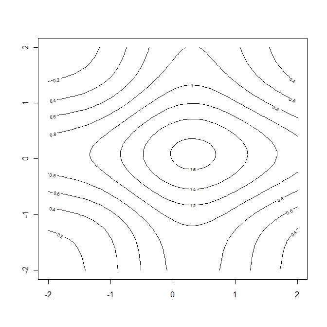
Because the performance of the estimators depends on the correct specification of the convolution function $\psi$ we next investigate the performance of the estimators under misspecification of the function $\psi$ . In Figure 3 we display the contour plots of the estimates $\hat{\theta}^{add,FD}$ , where in every panel the convolution function is misspecificated as Laplace distribution $Lap(\alpha,\beta)$ with parameters $\alpha=0$ and $\beta=\frac{1}{3}$ . In the upper left and upper right panel the $\beta$ parameter of the Laplace distribution $Lap(\alpha,\beta)$ is misspecificated, whereas in the lower left panel the true convolution function is the density of a standard normal distribution and in the lower right panel it is a gamma distribution. We observe, that a miss-specification of the shape of the convolution function (as it occurs if a Laplace density is used instead of the density of a Gamma(3,2) distribution) yields to an estimator with a different structure as the true signal (see the lower right panel in Figure 3). All other panels show the same structure as the upper left panel Figure 2 which gives the contour plot of the true signal $\theta^{(1)}$ . This indicates that the structure of the signal can be reconstructed, as long as the chosen convolution kernel exhibits similar modal properties as the “true kernel” . However, we also observe from Figure 3 that the levels of the contour differ from those of the true signal.

We conclude this section with a brief discussion of the performance of the unrestricted estimator $\hat{\theta}^{RD}$ under the assumption (RD) of a non-uniform random design. In Table 3 we display the simulated mean, variance and mean squared error for various distributions of the predictor $\bf{X}$ , where the components are independent and identically distributed. In most cases we observe similar results for the bias, independently of the distribution of $\bf{X}$ and the choice of the sequence $a_{n}$ . On the other hand the mean squared error is dominated by the variance, which depends sensitively on the choice of the parameter $a_{n}$ . This observation corresponds with the representation of the asymptotic variance of $\hat{\theta}^{RD}$ in formula (3.3) of Theorem 3.1. We also observe that the impact of the distribution of the explanatory variable on the variance of the estimate $\hat{\theta}^{RD}$ is much smaller.

${\bf X}$	$N$	$a_{n}$	$x_{1}$	$x_{2}$	$\theta^{(1)}(\textbf{x})$	$\mathbb{E}\hat{\theta}(\textbf{x})$	Var $\hat{\theta}(\textbf{x})$	MSE $\hat{\theta}(\textbf{x})$
	10201	0.25	0	0	1.8422	1.7421	0.0297	0.0397
$U[\frac{-1}{a_{n}},\frac{1}{a_{n}}]$	10201	0.25	0	1	1.6877	1.7163	0.0272	0.0283
	10201	0.25	1	1	1.1425	1.2858	0.0194	0.0399
	10201	0.25	1	1.8	0.5857	0.6105	0.0117	0.0123
	10201	0.5	0	0	1.8422	1.4957	0.0076	0.1277
$U[\frac{-1}{a_{n}},\frac{1}{a_{n}}]$	10201	0.5	0	1	1.6877	1.8123	0.0070	0.0225
	10201	0.5	1	1	1.1425	1.5438	0.0044	0.1654
	10201	0.5	1	1.8	0.5857	0.5695	0.0023	0.0026
	10201	0.25	0	0	1.8422	1.8512	0.3271	0.3271
$N(0,1)$	10201	0.25	0	1	1.6877	1.7019	0.7098	0.7100
	10201	0.25	1	1	1.1425	1.2038	0.7077	0.7115
	10201	0.25	1	1.8	0.5857	0.5983	0.4477	0.4479
	10201	0.5	0	0	1.8422	1.8229	0.0079	0.0083
$N(0,1)$	10201	0.5	0	1	1.6877	1.7466	0.0107	0.0143
	10201	0.5	1	1	1.1425	1.2531	0.0114	0.0236
	10201	0.5	1	1.8	0.5857	0.6366	0.0135	0.0161
	10201	0.25	0	0	1.8422	1.8758	0.0174	0.0185
$t(2)$	10201	0.25	0	1	1.6877	1.7129	0.0255	0.0261
	10201	0.25	1	1	1.1425	1.1786	0.0271	0.0284
	10201	0.25	1	1.8	0.5857	0.6138	0.0324	0.0332
	10201	0.5	0	0	1.8422	1.8590	0.0115	0.0118
$t(2)$	10201	0.5	0	1	1.6877	1.7260	0.0158	0.0173
	10201	0.5	1	1	1.1425	1.2069	0.0182	0.0223
	10201	0.5	1	1.8	0.5857	0.6275	0.0174	0.0191

Table 3: Mean, variance and mean squared error of the unrestricted estimator

\hat{\theta}^{RD}

proposed in this paper for different distributions of the explanatory variables

{\bf X}

and different choices for the parameter

a_{n}

. The model is given by (5.1) and the variance is

\sigma^{2}=0.25

Acknowledgements. This work has been supported in part by the Collaborative Research Center “Statistical modeling of nonlinear dynamic processes” (SFB 823, Teilprojekt C1, C4) of the German Research Foundation (DFG).

References

Adorf, (1995) Adorf, H. M. (1995). Hubble space telescope image restoration in its forth year. inverse problems. Inverse Problems, 11:639–653.
Bertero et al., (2009) Bertero, M., Boccacci, P., Desiderà, G., and Vicidomini, G. (2009). Image deblurring with Poisson data: From cells to galaxies. Inverse Problems, 25(12):123006, 26.
Birke and Bissantz, (2008) Birke, M. and Bissantz, N. (2008). Asymptotic normality and confidence intervals for inverse regression models with convolution-type operators. Journal of Multivariate Statistics, 100(10):2364–2375.
Birke et al., (2012) Birke, M., Bissantz, N., and Hildebrandt, T. (2012). Asymptotic normality and confidence intervals for time-dependent inverse regression models with convolution-type operators. Submitted for publication.
Birke et al., (2010) Birke, M., Bissantz, N., and Holzmann, H. (2010). Confidance bands for inverse regression models. Inverse Problems, 26:115020.
(6) Bissantz, N., Dümbgen, L., Holzmann, H., and Munk, A. (2007a). Nonparametric confidence bands in deconvolution density estimation. Journal of the Royal Statistical Society Series B, 69:483–506.
(7) Bissantz, N., Hohage, T., Munk, A., and Ruymgaart, F. (2007b). Convergence rates of general regularization methods for statistical inverse problems. SIAM J. Num. Anal., 45:2610–2636.
Brillinger, (2001) Brillinger, D. (2001). Time Series Data Analysis and Theory. SIAM.
Carroll et al., (2002) Carroll, R. J., Härdle, W., and Mammen, E. (2002). Estimation in an additive model when the parameters are linked parametrically. Econometric Theory, 18(4):886–912.
Cavalier, (2008) Cavalier, L. (2008). Nonparametric statistical inverse problems. Inverse Problems, 24(3):034004, 19.
Cavalier and Tsybakov, (2002) Cavalier, L. and Tsybakov, A. (2002). Sharp adaption for inverse problems with random noise. Prob. Theory Related Fields, 123:323–354.
De Gooijer and Zerom, (2003) De Gooijer, J. G. and Zerom, D. (2003). On additive conditional quantiles with high-dimensional covariates. Journal of the American Statistical Association, 98(461):135–146.
Dette and Scheder, (2011) Dette, H. and Scheder, R. (2011). Estimation of additive quantile regression. Annals of the Institute of Statistical Mathematics, 63(2):245–265.
Diggle and Hall, (1993) Diggle, P. J. and Hall, P. (1993). A fourier approach to nonparametric deconvolution of a density estimate. Journal of the Royal Statistical Society Series B, 55:523–531.
Doksum and Koo, (2000) Doksum, K. and Koo, J. Y. (2000). On spline estimators and prediction intervals in nonparametric regression. Computational Statistics and Data Analysis, 35:67–82.
Engl et al., (1996) Engl, H. W., Hanke, M., and Neubauer, A. (1996). Regularization of inverse problems, volume 375 of Mathematics and its Applications. Kluwer Academic Publishers Group, Dordrecht.
Fan, (1991) Fan, J. (1991). On the optimal rates of convergence for nonparametric deconvolution problems. Annals of Statistics., 19:1257–1272.
Hastie and Tibishirani, (2008) Hastie, T. and Tibishirani, R. (2008). Generalized additive models. Chapman & Hall.
Hengartner and Sperlich, (2005) Hengartner, N. W. and Sperlich, S. (2005). Rate optimal estimation with the integration method in the presence of many covariates. Journal of Multivariate Analysis, 95(2):246–272.
Horowitz and Lee, (2005) Horowitz, J. and Lee, S. (2005). Nonparametric estimation of an additive quantile regression model. Journal of the American Statistical Association, 100(472):1238–1249.
Kaipio and Somersalo, (2010) Kaipio, J. and Somersalo, E. (2010). Statistical and Computational Inverse Problems. Springer, Berlin.
Lee et al., (2010) Lee, Y. K., Mammen, E., and U., P. B. (2010). Backfitting and smooth backfitting for additive quantile models. Annals of Statistics, 38(5):2857–2883.
(23) Linton, O. and Nielsen, J. (1995a). A kernel method of estimating structured nonparametric regression based on marginal integration. Biometrika, 82(1):93–100.
(24) Linton, O. B. and Nielsen, J. P. (1995b). A kernel method of estimating structured nonparametric regression based on marginal integration. Biometrika, 82(1):93–100.
Mair and Ruymgaart, (1996) Mair, B. A. and Ruymgaart, F. H. (1996). Statistical inverse estimation in Hilbert scales. SIAM J. Appl. Math., 56:1424–1444.
Mammen et al., (1999) Mammen, E., Linton, O. B., and Nielsen, J. (1999). The existence and asymptotic properties of a backfitting projection algorithm under weak conditions. Annals of Statistics, 27(5):1443–1490.
Nielsen and Sperlich, (2005) Nielsen, J. P. and Sperlich, S. (2005). Smooth backfitting in practice. Journal of the Royal Statistical Society, Ser. B, 67(1):43–61.
Saitoh, (1997) Saitoh, S. (1997). Integral Transforms, Reproducing Kernels and their Applications. Longman, Harlow.
Stefanski and Carroll, (1990) Stefanski, L. and Carroll, R. (1990). Deconvoluting kernel density estimators. Statistics, 21:169–184.

6 Appendix

For the proofs we make frequent use of the cumulant method, which is a common tool in time series analysis. Following Brillinger, (2001) the $r$ -th order joint cumulant $cum(Y_{1},...,Y_{r})$ of a $r$ -dimensional complex valued random vector $(Y_{1},...,Y_{r})$ is given by

(5.1)

\displaystyle cum(Y_{1},...,Y_{r})

\displaystyle=

\displaystyle\sum(-1)^{p-1}(p-1)!\Big(E\prod_{j\in\nu_{1}}Y_{j}\Big)\dots\Big(E\prod_{j\in\nu_{p}}Y_{j}\Big),

where we assume the existence of moments of order $r$ , i.e. $E(|Y_{j}^{r}|)<\infty$ $(j=1,...,r)$ and the summation extends over all partitions $(\nu_{1},...,\nu_{p}),p=1,...,r$ of $(1,...,r)$ . If we choose $Y_{j}=Y,j=1,...,r$ we denote with $cum_{r}(Y)=cum(Y,...,Y)$ the $r$ -th order cumulant of a univariate random variable. The following properties of the cumulant will be used frequently in our proofs [see e.g. Brillinger, (2001)].

(B1)

$cum(a_{1}Y_{1},...,a_{r}Y_{r})=a_{1}\dots a_{r}cum(Y_{1},...,Y_{r})$ for constants $a_{1},...,a_{r}\in\mathbb{C}$
(B2)

if any group of the Y’s is independent of the remaining Y’s, then $cum(Y_{1},...,Y_{r})=0$
(B3)

for the random variable $(Z_{1},Y_{1},...,Y_{r})$ we have

$cum(Z_{1}+Y_{1},Y_{2},...,Y_{r})=cum(Z_{1},Y_{2},...,Y_{r})+cum(Y_{1},Y_{2},...,Y_{r})$
(B4)

if the random variables $(Y_{1},...,Y_{r})$ and $(Z_{1},...,Z_{r})$ are independent, then

$cum(Y_{1}+Z_{1},...,Y_{r}+Z_{r})=cum(Y_{1},...,Y_{r})+cum(Z_{1},...,Z_{r})$
(B5)

$cum(Y_{j})=E(Y_{j})$ for $j=1,...,r$
(B6)

$cum(Y_{j},\overline{Y}_{j})=Var(Y_{j})$ for $j=1,...,r$

We finally state a result which can easily be proven by using the definition (5.1) and the properties of the mean.

Theorem 6.1.

Let $\textbf{Y}=(Y_{1},...,Y_{r})$ be a random variable, $b_{n}$ a sequence and $C>0$ a constant with

\displaystyle E\Big[\prod_{j=1}^{l}|Y_{i_{j}}|\Big]

\displaystyle\leq

\displaystyle C^{l}b_{n}^{l}\qquad\mbox{for all }1\leq l\leq r,

then $|cum(Y_{i_{1}},...,Y_{i_{m}})|\leq(m-1)!C^{m}b_{n}^{m}\sum_{j=1}^{m}S_{m,j},$ where $S_{m,j}$ denotes the Sterling number of the second kind.

We will also make use of the fact that the normal distribution with mean $\mu$ and variance $\sigma^{2}$ is characterized by its cumulants, where the first two cumulants are equal to $\mu$ and $\sigma^{2}$ respectively and all cumulants of larger order are zero. To show asymptotic normality in our proofs we have to calculate the first two cumulants which give the asymptotic mean and variance and show in a second step that all cumulants of order $l\geq 3$ are vanishing asymptotically. In the following discussion all constants which do not depend on the sample size (but may differ in different steps of the proofs) will be denoted by $C$ .

Proof of Theorem 3.1: For the sake of brevity we write $\hat{\theta}$ instead of $\hat{\theta}^{full,RD}$ throughout this proof. By the discussion of the previous paragraph we have to calculate the mean and the variance of $\hat{\theta}(\textbf{x}^{*})$ and all cumulants of order $l\geq 3$ . We start with the mean conditional on $\textbf{X}=(\textbf{X}_{1},...,\textbf{X}_{n})$ , which can be calculated as

\displaystyle E[\hat{\theta}(\textbf{x}^{*})|\textbf{X}]

\displaystyle=

\displaystyle\sum_{k=1}^{n}g(\textbf{X}_{k})w_{n}(\textbf{x}^{*},\textbf{X}_{k})

where the weights $w_{n}$ are defined in (2.6). By iterative expectation we get

\displaystyle E[\hat{\theta}(\textbf{x}^{*})]

\displaystyle=

\displaystyle\frac{1}{h^{d}(2\pi)^{d}}\int_{\mathbb{R}^{d}}g(\textbf{x})\int_{\mathbb{R}^{d}}e^{-i\langle\textbf{s},(\textbf{x}^{*}-\textbf{x})\rangle/h}\frac{\Phi_{K}(\textbf{s})}{\Phi_{\psi}(\frac{\textbf{s}}{h})}\frac{f(\textbf{x})}{\max\{f(\textbf{x}),f(\frac{1}{\bf{a}_{n}})\}}d\textbf{s}d\textbf{x},

which yields a bias of the form $bias_{\hat{\theta}}=E[\hat{\theta}(\textbf{x}^{*})]-\theta(\textbf{x}^{*})=A_{1}+A_{2},$ where (note that $\Phi_{g}=\Phi_{\psi}\cdot\Phi_{\theta}$ )

	$\displaystyle A_{1}$	$\displaystyle=$	$\displaystyle\frac{1}{h^{d}(2\pi)^{d}}\int_{\mathbb{R}^{d}}e^{-i\langle\textbf{s},\textbf{x}^{}\rangle/h}\Phi_{K}(\textbf{s})\Phi_{\theta}\left(\frac{\textbf{s}}{h}\right)d\textbf{s}-\theta(\textbf{x}^{})$
	$\displaystyle A_{2}$	$\displaystyle=$	$\displaystyle\frac{1}{h^{d}(2\pi)^{d}}\int_{\mathbb{R}^{d}}e^{-i\langle\textbf{s},\textbf{x}^{*}\rangle/h}\frac{\Phi_{K}(\textbf{s})}{\Phi_{\psi}(\frac{\textbf{s}}{h})}\int_{\mathbb{R}^{d}}g(\textbf{x})e^{i\langle s,\textbf{x}\rangle/h}\Big(\frac{f(\textbf{x})}{\max\{f(\textbf{x}),f(\frac{1}{\bf{a}_{n}})\}}-1\Big)d\textbf{x}d\textbf{s}$

For the summand $A_{1}$ we can use exactly the same calculation as in Birke and Bissantz, (2008) to obtain $A_{1}=O(h^{s-1})$ . For the second term $A_{2}$ we have

	$\displaystyle A_{2}$	$\displaystyle\leq$	$\displaystyle\frac{1}{h^{d}(2\pi)^{d}}\int_{\mathbb{R}^{d}}\frac{\|\Phi_{K}(\textbf{s})\|}{\|\Phi_{\psi}(\frac{\textbf{s}}{h})\|}\int_{\mathbb{R}^{d}}\|g(\textbf{x})\|\Big\|\frac{f(\textbf{x})}{\max\{f(\textbf{x}),f(\frac{1}{\bf{a}_{n}})\}}-1\Big\|d\textbf{x}d\textbf{s}$
		$\displaystyle\leq$	$\displaystyle\frac{C}{h^{d+\beta}(2\pi)^{d}}\int_{([-\frac{1}{a_{n}},\frac{1}{a_{n}}]^{d})^{c}}\|g(\textbf{x})\|\Big\|\frac{f(\textbf{x})}{\max\{f(\textbf{x}),f(\frac{1}{\bf{a}_{n}})\}}-1\Big\|d\textbf{x},$

where we used Assumption 1(A) and 4 in the last inequality. In the next step we will use the fact that $0\leq\frac{f(\textbf{x})}{\max\left\{f(\textbf{x}),f(\frac{1}{\bf{a}_{n}})\right\}}\leq 1$ ( $\textbf{x}\in\mathbb{R}^{d}$ ) and Assumption 3(B) to obtain

\displaystyle A_{2}

\displaystyle\leq

\displaystyle\frac{C}{h^{d+\beta}(2\pi)^{d}}\int_{([-\frac{1}{a_{n}},\frac{1}{a_{n}}]^{d})^{c}}|g(\textbf{x})|\parallel\textbf{x}\parallel^{r}\frac{1}{\parallel\textbf{x}\parallel^{r}}d\textbf{x}=O\Big(\frac{a_{n}^{r}}{h^{d+\beta}}\Big)=O(h^{s-1}).

This shows that the bias of $\hat{\theta}(\textbf{x}^{*})$ is of order $O(h^{s-1})$ . By the definition of $\hat{\theta}(\textbf{x}^{*})$ and (2.6) it follows

\displaystyle V(\hat{\theta}(\textbf{x}^{*})|\textbf{X})

\displaystyle=

\displaystyle\frac{\sigma^{2}}{n^{2}h^{2d}(2\pi)^{2d}}\sum_{k=1}^{n}\Big|\int_{\mathbb{R}^{d}}e^{-i\langle\textbf{s},(\textbf{x}^{*}-\textbf{X}_{k})\rangle/h}\frac{\Phi_{K}(\textbf{s})}{\Phi_{\psi}(\frac{\textbf{s}}{h})}d\textbf{s}\Big|^{2}\frac{1}{\max\{f(\textbf{X}_{k}),f(\frac{1}{\bf{a}_{n}})\}^{2}}

which yields

\displaystyle E[V(\hat{\theta}(\textbf{x}^{*})|\textbf{X})]

\displaystyle=

\displaystyle\frac{\sigma^{2}}{nh^{d}(2\pi)^{2d}}\int_{\mathbb{R}^{d}}\Big|\int_{\mathbb{R}^{d}}e^{-i\langle\textbf{s},(\textbf{x}^{*}/h-y)\rangle}\frac{\Phi_{K}(\textbf{s})}{\Phi_{\psi}(\frac{\textbf{s}}{h})}d\textbf{s}\Big|^{2}\frac{f(h\textbf{y})}{\max\{f(h\textbf{{y}}),f(\frac{1}{\bf{a}_{n}})\}^{2}}d\textbf{y}.

The variance of the conditional expectation is given by (observe again the definition of the weight $w_{n}$ in (2.6))

$\displaystyle V(E[\hat{\theta}(\textbf{x}^{*})\|\textbf{X}])$	$\displaystyle=$	$\displaystyle V\Big(\sum_{k=1}^{n}g(\textbf{X}_{k})w_{n}(\textbf{x}^{*},\textbf{X}_{k})\Big)$
	$\displaystyle=$	$\displaystyle\frac{1}{nh^{d}(2\pi)^{2d}}\int_{\mathbb{R}^{d}}\Big\|\int_{\mathbb{R}^{d}}e^{-i\langle\textbf{s},(\textbf{x}^{*}/h-\textbf{y})\rangle}\frac{\Phi_{K}(\textbf{s})}{\Phi_{\psi}(\frac{\textbf{s}}{h})}d\textbf{s}\Big\|^{2}\frac{g^{2}(h\textbf{y})f(h\textbf{y})}{\max\{f(h\textbf{{y}}),f(\frac{1}{\bf{a}_{n}})\}^{2}}d\textbf{y}$
	$\displaystyle-$	$\displaystyle\frac{1}{n(2\pi)^{2d}}\Big\|\int_{\mathbb{R}^{d}}\int_{\mathbb{R}^{d}}e^{-i\langle\textbf{s},(\textbf{x}^{*}/h-\textbf{y})\rangle}\frac{\Phi_{K}(\textbf{s})}{\Phi_{\psi}(\frac{\textbf{s}}{h})}d\textbf{s}\frac{g(h\textbf{y})f(h\textbf{y})}{\max\big\{f(h\textbf{{y}}),f(\frac{1}{\bf{a}_{n}})\big\}}d\textbf{y}\Big\|^{2},$

where the second summand is of order $O(n^{-1})$ . Thus the variance can be written as

(5.2)				$\displaystyle V(\hat{\theta}(\textbf{x}^{}))=E[V(\hat{\theta}(\textbf{x}^{})\|\textbf{X})]+V(E[\hat{\theta}(\textbf{x}^{*})\|\textbf{X}])$
(5.2)			$\displaystyle=$	$\displaystyle\frac{1}{nh^{d}(2\pi)^{2d}}\int_{\mathbb{R}^{d}}\Big\|\int_{\mathbb{R}^{d}}e^{-i\langle\textbf{s},(\textbf{x}^{*}/h-y)\rangle}\frac{\Phi_{K}(\textbf{s})}{\Phi_{\psi}(\frac{\textbf{s}}{h})}d\textbf{s}\Big\|^{2}\frac{(\sigma^{2}+g^{2}(h\textbf{y}))f(h\textbf{y})}{\max\{f(h\textbf{{y}}),f(\frac{1}{\bf{a}_{n}})\}^{2}}d\textbf{y}+O(n^{-1})$

and the rate of convergence has a lower bound given by

V(\hat{\theta}(\textbf{x}^{*}))^{-1/2}=\Omega\big(n^{1/2}h^{\beta+d/2}f(\textbf{a}_{\textbf{n}}^{-1})^{1/2}\big),

where the symbol $b_{n}=\Omega(c_{n})$ means that there exists a constant $C$ and $n_{0}\in\mathbb{N}$ such that for all $n\geq n_{0}$ we have $|b_{n}|\geq C|c_{n}|$ . The variance has a lower bound

	$\displaystyle V(\hat{\theta}(\textbf{x}^{*}))$	$\displaystyle\geq$	$\displaystyle\frac{1}{nh^{d}(2\pi)^{2d}}\int_{([\frac{-1}{ha_{n}},\frac{1}{ha_{n}}]^{d})}\Big\|\int_{\mathbb{R}^{d}}e^{-i\langle\textbf{s},(\textbf{x}^{*}/h-y)\rangle}\frac{\Phi_{K}(\textbf{s})}{\Phi_{\psi}(\frac{\textbf{s}}{h})}d\textbf{s}\Big\|^{2}\frac{(\sigma^{2}+g^{2}(h\textbf{y}))f(h\textbf{y})}{f(h\textbf{{y}})^{2}}d\textbf{y}$
		$\displaystyle\geq$	$\displaystyle\frac{C}{nh^{d}(2\pi)^{2d}}\int_{([\frac{-1}{ha_{n}},\frac{1}{ha_{n}}]^{d})}\Big\|\int_{\mathbb{R}^{d}}e^{-i\langle\textbf{s},(\textbf{x}^{*}/h-y)\rangle}\frac{\Phi_{K}(\textbf{s})}{\Phi_{\psi}(\frac{\textbf{s}}{h})}d\textbf{s}\Big\|^{2}d\textbf{y}=C(nh^{d+2\beta})^{-1}(1+o(1)),$

where we used Assumption 4 and Parsevals equality. This yields to the upper bound

(5.3)

\displaystyle V(\hat{\theta}(\textbf{x}^{*}))^{-1/2}

\displaystyle=

\displaystyle O\left(n^{1/2}h^{\beta+d/2}\right)

For the proof of asymptotic normality we now show that the $l$ -th cumulant of $G_{l}=\big|cum_{l}\big(V(\hat{\theta}(x^{*}))^{-1/2}\hat{\theta}(\textbf{x}^{*})\big)\big|$ is vanishing asymptotically, whenever $l\geq 3$ . For this purpose we recall the definition of the weights $w_{n}$ in (2.6) and obtain from (5.3) the estimate

(5.4)	$\displaystyle G_{l}$	$\displaystyle\leq$	$\displaystyle Cn^{l/2}h^{l\beta+dl/2}\sum_{k_{1},...,k_{l}=1}^{n}\|cum\big(Y_{k_{1}}w_{n}(\textbf{x}^{},\textbf{X}_{k_{1}}),...,Y_{k_{l}}w_{n}(\textbf{x}^{},\textbf{X}_{k_{l}})\big)\|$
		$\displaystyle=$	$\displaystyle Cn^{l/2}h^{l\beta+dl/2}\sum_{k=1}^{n}\|cum_{l}\big(Y_{k}w_{n}(\textbf{x}^{*},\textbf{X}_{k})\big)\|$
		$\displaystyle=$	$\displaystyle Cn^{l/2+1}h^{l\beta+dl/2}\sum_{\textbf{j}\in\{0,1\}^{l}}\|(cum(U^{j_{1}}w_{n}(\textbf{x}^{},\textbf{X}_{1}),...,U^{j_{l}}w_{n}(\textbf{x}^{},\textbf{X}_{1}))\|,$

where we used (B2) and the notation $U^{0}=g(\textbf{X}_{1})$ and $U^{1}=\varepsilon$ . This term can be written as

\displaystyle Cn^{l/2+1}h^{l\beta+dl/2}\sum_{s=0}^{l}\dbinom{l}{s}\sum_{\begin{subarray}{c}\textbf{j}\in\{0,1\}^{l}\\ j_{1}+...+j_{l}=s\end{subarray}}\big|cum(U^{j_{1}}w_{n}(\textbf{x}^{*},\textbf{X}_{1}),...,U^{j_{l}}w_{n}(\textbf{x}^{*},\textbf{X}_{1}))\big|.

By using the product theorem for cumulants [see e.g. Brillinger, (2001)], we obtain

(5.5)

\displaystyle Cn^{l/2+1}h^{l\beta+dl/2}\sum_{s=0}^{l}\dbinom{l}{s}\sum_{\begin{subarray}{c}\textbf{j}\in\{0,1\}^{l}\\ j_{1}+...+j_{l}=s\end{subarray}}\Big|\sum_{\nu}\prod_{k=1}^{p}cum(A_{ij},ij\in\nu_{k})\Big|,

where the third sum is calculated over all indecomposable partitions $\nu=(\nu_{1},...,\nu_{p})$ of the table

$A_{i1}$		$A_{i2}$
⋮		⋮
$A_{i1}$		$A_{i2}$
	$A_{ij}$
	⋮
	$A_{ij}$

(here the first $s$ rows have two and the last $l-s$ rows have one column) and

$\displaystyle A_{i1}$	$\displaystyle=$	$\displaystyle\varepsilon\qquad\qquad\qquad\qquad\;1\leq i\leq s$
$\displaystyle A_{i2}$	$\displaystyle=$	$\displaystyle w_{n}(\textbf{x}^{*},\textbf{X}_{1}))\qquad\qquad 1\leq i\leq s$
$\displaystyle A_{ij}$	$\displaystyle=$	$\displaystyle g(\textbf{X}_{1})w_{n}(\textbf{x}^{*},\textbf{X}_{1}))\qquad s+1\leq i\leq l.$

As $\varepsilon$ is independent of X only those indecomposable partitions yield a non zero cumulant, which seperate all $\varepsilon$ ’s from the other terms. This means that for a partition $\nu$ there are $m(\nu)$ sets $\nu_{1},...,\nu_{m(\nu)}$ which include only $\varepsilon^{\prime}s$ while $\nu_{m(\nu)+1},...,\nu_{p}$ contain only $w_{n}(\textbf{x}^{*},\textbf{X})$ ’s and $g(\textbf{X})w_{n}(\textbf{x}^{*},\textbf{X})$ ’s. Thus (5.5) can be written as

(5.6)

\displaystyle Cn^{l/2+1}h^{l\beta+dl/2}\sum_{s=0}^{l}\dbinom{l}{s}\sum_{\begin{subarray}{c}\textbf{j}\in\{0,1\}^{l}\\ j_{1}+...+j_{l}=s\end{subarray}}\Big|\sum_{\nu}\prod_{k=1}^{m(\nu)}cum_{s_{k}}(\varepsilon)\prod_{k=m(\nu)+1}^{p}cum(A_{ij},ij\in\nu_{k})\Big|

with

	$\displaystyle A_{ij}$	$\displaystyle=$	$\displaystyle w_{n}(\textbf{x}^{*}-\textbf{X}_{1}))\qquad\qquad 1\leq i\leq s$
	$\displaystyle A_{ij}$	$\displaystyle=$	$\displaystyle g(\textbf{X})w_{n}(\textbf{x}^{*}-\textbf{X}_{1}))\qquad s+1\leq i\leq l.$

and $s_{1}+...+s_{m(\nu)}=s$ . Furthermore we have $s_{i}\geq 2$ , because the noise terms $\varepsilon$ have mean zero, and each set $\nu_{m(\nu)+1},...,\nu_{p}$ includes at least one $A_{ij}$ with $1\leq i\leq s$ because otherwise the partition would not be indecomposable. Let $a_{r}=|\nu_{r}|$ denote the number of elements in the set $\nu_{r}\mbox{ }(r=m(\nu)+1,...,p)$ , then we get $a_{m+1}+...+a_{p}=l$ . Furthermore for $r\in\{m+1,...,p\}\mbox{ the cumulant }cum(A_{ij},ij\in\nu_{r})$ equals

(5.7)

\displaystyle cum(g(\textbf{X}_{1})w_{n}(\textbf{x}^{*},\textbf{X}_{1})),...,g(\textbf{X}_{1})w_{n}(\textbf{x}^{*},\textbf{X}_{1})),w_{n}(\textbf{x}^{*},\textbf{X}_{1})),...,w_{n}(\textbf{x}^{*},\textbf{X}_{1})))

because of the symmetry of the arguments in the cumulant. In the next step we denote by $b_{r}$ the number of components of the form $g(\textbf{X}_{1})w_{n}(\textbf{x}^{*},\textbf{X}_{1})$ and show the estimate

(5.8)

\displaystyle E\Big[\prod_{i=1}^{b_{r}}|g(\textbf{X}_{1})w_{n}(\textbf{x}^{*},\textbf{X}_{1}))|\prod_{j=1}^{a_{r}-b_{r}}|w_{n}(\textbf{x}^{*},\textbf{X}_{1}))|\Big]\leq\frac{C^{a_{r}}}{n^{a_{r}}h^{a_{r}(\beta+d)}f(\frac{1}{\bf{a}_{n}})^{a_{r}}}

(which does not depend on $b_{r}$ ). From Theorem 5.1 we then obtain that the term in (5.7) is of order $O(n^{-a_{r}}h^{-a_{r}(\beta+d)}f(1/\textbf{a}_{\textbf{n}})^{-a_{r}})$ . Equations (5.4), (5.6) and (5.7) yield for the cumulants of order $l\geq 3$

	$\displaystyle G_{l}$	$\displaystyle\leq$	$\displaystyle Cn^{l/2+1}h^{l\beta+dl/2}\sum_{s=0}^{l}\dbinom{l}{s}\sum_{\begin{subarray}{c}\textbf{j}\in\{0,1\}^{l}\\ j_{1}+...+j_{l}=s\end{subarray}}\Big\|\sum_{\nu}\prod_{k=1}^{m(\nu)}cum_{s_{k}}(\varepsilon)\prod_{r=m(\nu)+1}^{p}\frac{C^{a_{r}}}{n^{a_{r}}h^{a_{r}(d+\beta)}f(\frac{1}{\bf{a}_{n}})^{a_{r}}}\Big\|$
		$\displaystyle=$	$\displaystyle O\big((n^{l/2-1}h^{ld/2}f({\bf{a}_{n}}^{-1})^{l})^{-1}\big)=o(1),$

which shows the asymptotic normality.
In order to prove the remaining estimate (5.8) we use the definition of $w_{n}(\textbf{x}^{*},\textbf{X}_{1})$ and obtain for the term on the left hand side of (5.8)

$\displaystyle L_{n}$	$\displaystyle=$	$\displaystyle\int_{\mathbb{R}^{d}}\|g(\textbf{x})\|^{b_{r}}\Big(\frac{1}{nh^{d}(2\pi)^{d}}\Big\|\int_{\mathbb{R}^{d}}e^{-i\langle\textbf{s},(\textbf{x}^{*}-\textbf{x})\rangle/h}\frac{\Phi_{K}(\textbf{s})}{\Phi_{\psi}(\frac{\textbf{s}}{h})}\frac{1}{\max\{f(\textbf{x}),f(\frac{1}{\bf{a}_{n}})\}}d\textbf{s}\Big\|\Big)^{a_{r}}f(\textbf{x})d\textbf{x}$
	$\displaystyle\leq$	$\displaystyle\frac{C}{n^{a_{r}}h^{a_{r}d}}\int_{\mathbb{R}^{d}}\|g(\textbf{x})\|^{b_{r}}\Big(\int_{\mathbb{R}^{d}}\frac{\|\Phi_{K}(\textbf{s})\|}{\|\Phi_{\psi}(\frac{\textbf{s}}{h})\|}\frac{1}{\max\{f(\textbf{x}),f(\frac{1}{\bf{a}_{n}})\}}d\textbf{s}\Big)^{a_{r}}f(\textbf{x})d\textbf{x}$
	$\displaystyle\leq$	$\displaystyle\frac{C}{n^{a_{r}}h^{a_{r}d}f(\frac{1}{\bf{a}_{n}})^{a_{r}}}\int_{\mathbb{R}^{d}}\Big(\int_{\mathbb{R}^{d}}\frac{\|\Phi_{K}(\textbf{s})\|}{\|\Phi_{\psi}(\frac{\textbf{s}}{h})\|}d\textbf{s}\Big)^{a_{r}}f(\textbf{x})d\textbf{x},$

where we used the fact that $g$ is bounded. Using this inequality and Assumption 1(A) it follows that $L_{n}\leq C/n^{a_{r}}h^{a_{r}(d+\beta)}f(\frac{1}{\bf{a}_{n}})^{a_{r}},$ which proves (5.8).

Proof of Lemma 3.3: Similar to the proof of Theorem 3.1, we have to calculate the cumulants of the estimators $\hat{\alpha}_{j,Q_{I_{j}^{c}}}(\textbf{x}_{I_{j}}^{*})$ . We start with the first order cumulant

\displaystyle E[\hat{\alpha}_{j,Q_{I_{j}^{c}}}(\textbf{x}_{I_{j}}^{*})]

\displaystyle=

\displaystyle\frac{1}{h^{d}(2\pi)^{d}}\int_{\mathbb{R}^{d-d_{j}}}\int_{\mathbb{R}^{d}}\int_{\mathbb{R}^{d}}g(\textbf{x})\int_{\mathbb{R}^{d}}\frac{\Phi_{K}(\textbf{s})}{\Phi_{\psi}(\frac{\textbf{s}}{h})}\frac{e^{-i\langle\textbf{s},(\textbf{x}^{*}-\textbf{x})\rangle/h}f(\textbf{x})}{\max\{f(\textbf{x}),f(\frac{1}{\bf{a}_{n}})\}}d\textbf{s}d\textbf{x}dQ_{I_{j}^{c}}(\textbf{x}_{I_{j}^{c}}^{*})

and with the same arguments as in the proof of Theorem 3.1, we obtain a bias of order $O(h^{s-1})$ . For the calculation of the variance of $\hat{\alpha}_{j,Q_{I_{j}^{c}}}(\textbf{x}_{I_{j}}^{*})$ we investigate its conditional variance. Recalling the definitions (2.6) and (2.20) it follows by a straightforward argument

	$\displaystyle V(\hat{\alpha}_{j,Q_{I_{j}^{c}}}(\textbf{x}_{I_{j}}^{*})\|\textbf{X})$	$\displaystyle=$	$\displaystyle\frac{\sigma^{2}}{n^{2}h^{2d}(2\pi)^{2d}}\sum_{k=1}^{n}\Big\|\int_{\mathbb{R}^{d}}e^{-i\langle\textbf{w},\textbf{X}_{k}\rangle/h}e^{i\langle\textbf{w}_{I_{j}},\textbf{x}_{I_{j}}\rangle/h}L_{I_{j}^{c}}\Big(\frac{\textbf{w}_{I_{j}^{c}}}{h}\Big)\frac{\Phi_{K}(\textbf{w})}{\Phi_{\psi}(\frac{\textbf{w}}{h})}d\textbf{w}\Big\|^{2}$
			$\displaystyle\times\frac{1}{\max\{f(\textbf{X}_{k}),f(\frac{1}{\bf{a}_{n}})\}^{2}},$

which gives

	$\displaystyle E\big[V(\hat{\alpha}_{j,Q_{I_{j}^{c}}}(\textbf{x}_{I_{j}}^{*})\|\textbf{X})\big]$	$\displaystyle=$	$\displaystyle\frac{\sigma^{2}}{nh^{2d}(2\pi)^{2d}}\int_{\mathbb{R}^{d}}\Big\|\int_{\mathbb{R}^{d}}e^{-i\langle\textbf{w},\textbf{x}\rangle/h}e^{i\langle\textbf{w}_{I_{j}},\textbf{x}_{I_{j}}\rangle/h}L_{I_{j}^{c}}\Big(\frac{\textbf{w}_{I_{j}^{c}}}{h}\Big)\frac{\Phi_{K}(\textbf{w})}{\Phi_{\psi}(\frac{\textbf{w}}{h})}d\textbf{w}\Big\|^{2}$
			$\displaystyle\times\frac{f(\textbf{x})}{\max\{f(\textbf{x}),f(\frac{1}{\bf{a}_{n}})\}^{2}}d\textbf{x}.$

The variance of the conditional expectation can be calculated as

$\displaystyle V\big(E[\hat{\alpha}_{j,Q_{I_{j}^{c}}}(\textbf{x}_{I_{j}}^{*})\|\textbf{X}]\big)$	$\displaystyle=$	$\displaystyle\frac{1}{nh^{d}(2\pi)^{2d}}\int_{\mathbb{R}^{d}}\Big\|\int_{\mathbb{R}^{d}}e^{-i\langle\textbf{w},\textbf{x}\rangle}e^{i\langle\textbf{w}_{I_{j}},\textbf{x}_{I_{j}}\rangle/h}L_{I_{j}^{c}}\Big(\frac{\textbf{w}_{I_{j}^{c}}}{h}\Big)\frac{\Phi_{K}(\textbf{w})}{\Phi_{\psi}(\frac{\textbf{w}}{h})}d\textbf{w}\Big\|^{2}$
		$\displaystyle\times\frac{g(h\textbf{x})^{2}f(h\textbf{x})}{\max\{f(h\textbf{x}),f(\frac{1}{\bf{a}_{n}})\}^{2}}d\textbf{x}$
	$\displaystyle-$	$\displaystyle\frac{1}{n(2\pi)^{2d}}\Big\|\int_{\mathbb{R}^{d}}\int_{\mathbb{R}^{d}}e^{-i\langle\textbf{w},\textbf{x}\rangle}e^{i\langle\textbf{w}_{I_{j}},\textbf{x}_{I_{j}}\rangle/h}L_{I_{j}^{c}}\Big(\frac{\textbf{w}_{I_{j}^{c}}}{h}\Big)\frac{\Phi_{K}(\textbf{w})}{\Phi_{\psi}(\frac{\textbf{w}}{h})}d\textbf{w}$
		$\displaystyle\times\frac{g(h\textbf{x})f(h\textbf{x})}{\max\{f(h\textbf{x}),f(\frac{1}{\bf{a}_{n}})\}}d\textbf{x}\Big\|^{2},$

where the second summand is of order $O(n^{-1})$ . Therefore it follows

	$\displaystyle V(\hat{\alpha}_{j,Q_{I_{j}^{c}}}(\textbf{x}_{I_{j}}^{*}))$	$\displaystyle=$	$\displaystyle\frac{1}{nh^{d}(2\pi)^{2d}}\int_{\mathbb{R}^{d}}\Big\|\int_{\mathbb{R}^{d}}e^{-i\langle\textbf{w},\textbf{y}\rangle}e^{i\langle\textbf{w}_{I_{j}},\textbf{x}_{I_{j}}\rangle/h}L_{I_{j}^{c}}\Big(\frac{\textbf{w}_{I_{j}^{c}}}{h}\Big)\frac{\Phi_{K}(\textbf{w})}{\Phi_{\psi}(\frac{\textbf{w}}{h})}d\textbf{w}\Big\|^{2}$
			$\displaystyle\times\frac{(\sigma^{2}+g(h\textbf{y})^{2})f(h\textbf{y})}{\max\{f(h\textbf{y}),f(\frac{1}{\bf{a}_{n}})\}^{2}}d\textbf{y}+O(n^{-1}).$

The upper bound for this term is obtained from Assumption 4 which gives

(5.9)

\displaystyle\frac{(\sigma^{2}+g(h\textbf{y})^{2})f(h\textbf{y})}{\max\{f(h\textbf{y}),f(\frac{1}{\bf{a}_{n}})\}^{2}}=O({\bf a_{n}}^{-1}).

Therefore an application of Parseval’s equality and Assumption 5(C) yields

(5.10)

\displaystyle V(\hat{\alpha}_{j,Q_{I_{j}^{c}}}(\textbf{x}_{I_{j}}^{*})\leq\frac{C}{nh^{d+2\beta-\gamma_{j}}f(\frac{1}{\bf{a}_{n}})}.

A similar argument as in the proof of Theorem 3.1 gives the lower bound $V(\hat{\alpha}_{j,Q_{I_{j}^{c}}}(\textbf{x}_{I_{j}}^{*})\geq C/nh^{d+2\beta-\gamma_{j}}.$ Finally the statement that the $l$ -th cumulant of $V(\hat{\alpha}_{j,Q_{I_{j}^{c}}}(\textbf{x}_{I_{j}}^{*})^{-1/2}\hat{\alpha}_{j,Q_{I_{j}^{c}}}(x_{I_{j}}^{*})$ is of order $o(1)$ can be shown by similiar arguments as in the proof of Theorem 3.1.

Proof of Theorem 3.5: The proof follows by similar arguments as given in the previous Sections. For the sake of brevity we restrict ourselves for the calculation of the first and second order cumulants. For this purpose we show, that the estimate $\hat{c}$ has a faster rate of convergence than $\hat{\alpha}_{j,Q_{I_{j}^{c}}}(\textbf{x}_{I_{j}}^{*})$ for at least one $j\in\{1,...,m\}$ . If this statement is correct the asymptotic variance of the statistic

\displaystyle\hat{\theta}^{add,RD}(\textbf{x}^{*})

\displaystyle=

\displaystyle\sum_{j=1}^{m}\hat{\alpha}_{j,Q_{I_{j}^{c}}}(\textbf{x}_{I_{j}}^{*})-(m-1)\hat{c}

is determined by its first term. Recalling the notation (2.12) this term has the representation

(5.11)

\displaystyle\hat{D}_{n}=\sum_{j=1}^{m}\hat{\alpha}_{j,Q_{I_{j}^{c}}}(\textbf{x}_{I_{j}}^{*})

\displaystyle=

\displaystyle\sum_{j=1}^{m}\sum_{k=1}^{n}Y_{k}w_{n}^{add,RD}(\textbf{x}_{I_{j}}^{*},\textbf{X}_{k})

and can be treated in the same way as before. The resulting bias of $\hat{D}_{n}$ is the sum of the biases of the individual term and therefore also of order $O(h^{s-1})$ . The conditional variance is given by

$\displaystyle V(\hat{D}_{n}\|\textbf{X})$	$\displaystyle=$	$\displaystyle\sigma^{2}\sum_{k=1}^{n}\Big\|\sum_{j=1}^{m}w_{n}^{add,RD}(\textbf{x}_{I_{j}}^{*},\textbf{X}_{k})\Big\|^{2}$
	$\displaystyle=$	$\displaystyle\frac{\sigma^{2}}{n^{2}h^{2d}(2\pi)^{2d}}\sum_{k=1}^{n}\Big\|\int_{\mathbb{R}^{d}}e^{i\langle\textbf{w},\textbf{X}_{k}\rangle/h}\Big(\sum_{j=1}^{m}e^{-i\langle\textbf{w}_{I_{j}},\textbf{x}_{I_{j}}^{*}\rangle/h}L_{I_{j}^{c}}\Big(\frac{\textbf{w}_{I_{j}^{c}}}{h}\Big)\Big)\frac{\Phi_{K}(\textbf{w})}{\Phi_{\psi}(\frac{\textbf{w}}{h})}d\textbf{w}$
		$\displaystyle\times\frac{1}{\max\{f(\textbf{X}_{k}),f(\frac{1}{\bf{a}_{n}})\}}\Big\|^{2}.$

This yields for expectation of the conditional variance

	$\displaystyle E\big[V(\hat{D}_{n}\|\textbf{X})\big]$
		$\displaystyle=$	$\displaystyle\frac{\sigma^{2}}{nh^{2d}(2\pi)^{2d}}\int_{\mathbb{R}^{d}}\Big\|\int_{\mathbb{R}^{d}}e^{i\langle\textbf{w},\textbf{s}\rangle/h}\Big(\sum_{j=1}^{m}e^{-i\langle\textbf{w}_{I_{j}},\textbf{x}_{I_{j}}^{*}\rangle/h}L_{I_{j}^{c}}\Big(\frac{\textbf{w}_{I_{j}^{c}}}{h}\Big)\Big)\frac{\Phi_{K}(\textbf{w})}{\Phi_{\psi}(\frac{\textbf{w}}{h})}d\textbf{w}\Big\|^{2}\frac{f(\textbf{s})}{\max\{f(\textbf{s}),f(\frac{1}{\bf{a}_{n}})\}^{2}}d\textbf{s}$

and the variance of the conditional expectation is obtained as

$\displaystyle V\big(E[\hat{D}_{n}\|\textbf{X}]\big)$
	$\displaystyle=$	$\displaystyle\frac{1}{nh^{d}(2\pi)^{2d}}\int_{\mathbb{R}^{d}}\Big\|\int_{\mathbb{R}^{d}}e^{i\langle\textbf{w},\textbf{s}\rangle}\Big(\sum_{j=1}^{m}e^{-i\langle\textbf{w}_{I_{j}},\textbf{x}_{I_{j}}^{*}\rangle/h}L_{I_{j}^{c}}\Big(\frac{\textbf{w}_{I_{j}^{c}}}{h}\Big)\Big)\frac{\Phi_{K}(\textbf{w})}{\Phi_{\psi}(\frac{\textbf{w}}{h})}d\textbf{w}\Big\|^{2}\frac{g(h\textbf{s})^{2}f(h\textbf{s})}{\max\{f(h\textbf{s}),f(\frac{1}{\bf{a}_{n}})\}^{2}}d\textbf{s}$
	$\displaystyle-$	$\displaystyle\frac{1}{n(2\pi)^{2d}}\Big\|\int_{\mathbb{R}^{d}}\int_{\mathbb{R}^{d}}e^{i\langle\textbf{w},\textbf{s}\rangle}\Big(\sum_{j=1}^{m}e^{-i\langle\textbf{w}_{I_{j}},\textbf{x}_{I_{j}}^{*}\rangle/h}L_{I_{j}^{c}}\Big(\frac{\textbf{w}_{I_{j}^{c}}}{h}\Big)\Big)\frac{\Phi_{K}(\textbf{w})}{\Phi_{\psi}(\frac{\textbf{w}}{h})}d\textbf{w}\frac{g(h\textbf{s})f(h\textbf{s})}{\max\{f(h\textbf{s}),f(\frac{1}{\bf{a}_{n}})\}}d\textbf{s}\Big\|^{2},$

where the second summand is of order $O(n^{-1})$ . Thus yields for the variance

	$\displaystyle V(\hat{D}_{n})$	$\displaystyle=$	$\displaystyle\frac{1}{nh^{2d}(2\pi)^{2d}}\int_{\mathbb{R}^{d}}\Big\|\int_{\mathbb{R}^{d}}e^{i\langle\textbf{w},\textbf{s}\rangle/h}\Big(\sum_{j=1}^{m}e^{-i\langle\textbf{w}_{I_{j}},\textbf{x}_{I_{j}}^{*}\rangle/h}L_{I_{j}^{c}}\Big(\frac{\textbf{w}_{I_{j}^{c}}}{h}\Big)\Big)\frac{\Phi_{K}(\textbf{w})}{\Phi_{\psi}(\frac{\textbf{w}}{h})}d\textbf{w}\Big\|^{2}$
			$\displaystyle\times\frac{(\sigma^{2}+g(\textbf{s})^{2})f(\textbf{s})}{\max\{f(\textbf{s}),f(\frac{1}{\bf{a}_{n}})\}}d\textbf{s}+O(n^{-1})$

In order to obtain bounds for the rate of the variance, we use the lower bound for $\max\{f(h\textbf{s}),f(\frac{1}{a_{n}})\}$ mentioned in (5.9) and Parseval’s equality which yields

\displaystyle\Big(\frac{1}{nh^{d}f(\frac{1}{\bf{a}_{n}})}\int_{\mathbb{R}^{d}}\left|\sum_{j=1}^{m}e^{-i\langle\textbf{w}_{I_{j}},\textbf{x}_{I_{j}}^{*}\rangle/h}L_{I_{j}^{c}}\Big(\frac{\textbf{w}_{I_{j}^{c}}}{h}\Big)\right|^{2}\frac{|\Phi_{K}(\textbf{w})|^{2}}{|\Phi_{\psi}(\frac{\textbf{w}}{h})|^{2}}d\textbf{w}\Big)^{1/2}

\displaystyle=

\displaystyle O\left((nh^{d+2\beta-\gamma_{min}}f(\bf{a}_{n}^{-1}))^{-1}\right)

as an upper bound, where the last estimate follows from Assumption 5. The lower bound is of order $\Omega((nh^{d+2\beta-\gamma_{min}})^{-1})$ , where we use Assumption 4 and the same calculations as in the previous Section. These are in fact the same bounds as for $\hat{\alpha}_{j^{*},Q_{I_{j^{*}}^{c}}}(\textbf{x}_{I_{j^{*}}}^{*})$ with $j^{*}=argmin_{j}\>\gamma_{j}$ . This means that

\hat{D}_{n}-E[\hat{D}_{n}]=O_{P}(n^{-1/2}h^{-d/2-\beta-\gamma_{min}/2}f({\bf a_{n}}^{-1})^{-1/2})

In the last step we show that the estimate $\hat{c}$ has a faster rate of convergence. For this purpose we write $\hat{c}$ as weighted sum of independent random variables that is

\displaystyle\hat{c}

\displaystyle=

\displaystyle\int_{\mathbb{R}^{d}}\hat{\theta}(\textbf{x}^{*})dQ(\textbf{x}^{*})=\frac{1}{nh^{d}(2\pi)^{d}}\sum_{k=1}^{n}\int_{\mathbb{R}^{d}}e^{i\langle\textbf{w},\textbf{X}_{k}\rangle/h}\Big(\prod_{j=1}^{m}L_{I_{j}^{c}}\Big(\frac{\textbf{w}_{I_{j}^{c}}}{h}\Big)\Big)\frac{\Phi_{K}(\textbf{w})}{\Phi_{\psi}(\frac{\textbf{w}}{h})}d\textbf{w}\frac{Y_{k}}{\max\{f(\textbf{X}_{k}),f(\frac{1}{\bf{a}_{n}})\}}

It now follows by similar calculations as given in the previous paragraph and Assumption 5(C) that

V(\hat{c})=o(V(\sum_{j=1}^{m}\hat{\alpha}_{j,Q_{I_{j}^{c}}}(\textbf{x}_{I_{j}}^{*})))

and thus we can ignore the term $\hat{c}$ for the calculation of the asymptotic variance of the statistic $\hat{\theta}^{add,RD}$ .

Proof of Lemma 3.6: Observing the representation (2.15) and (2.18) we decompose the estimator into its deterministic and stochastic part, that is

(5.12)

\displaystyle\hat{\theta}_{I_{j}}^{FD}(\textbf{x}_{I_{j}}^{*})

\displaystyle=

\displaystyle\hat{E}_{1n}+\hat{E}_{2n}

where

	$\displaystyle\hat{E}_{1n}$	$\displaystyle=$	$\displaystyle\frac{1}{(2n+1)^{d-d_{j}}}\sum_{\textbf{k}\in\{-n,...,n\}^{d}}(g_{I_{1}}(\textbf{z}_{\textbf{k}_{I_{1}}})+...+g_{I_{m}}(\textbf{z}_{\textbf{k}_{I_{m}}}))w_{\textbf{k}_{I_{j}},n}(\textbf{x}_{I_{j}}^{*})$
	$\displaystyle\hat{E}_{2n}$	$\displaystyle=$	$\displaystyle\frac{1}{(2n+1)^{d-d_{j}}}\sum_{\textbf{k}\in\{-n,...,n\}^{d}}^{n}\varepsilon_{\textbf{k}}w_{\textbf{k}_{I_{j}},n}(\textbf{x}_{I_{j}}^{*})$

and $w_{\textbf{k}_{I_{j}},n}(\textbf{x}_{I_{j}}^{*})$ are defined in (2.19). In a first step we show, that the bias of $\hat{\theta}_{I_{j}}^{FD}$ is of order $O(\frac{1}{n^{2}h^{2+d_{j}+\beta_{j}}a_{n}^{3}})$ . For this purpose we rewrite the deterministic part as

\displaystyle\hat{E}_{1n}

\displaystyle=

\displaystyle\hat{E}_{1n}^{(1)}+\hat{E}_{1n}^{(2)}

where

$\displaystyle\hat{E}_{1n}^{(1)}$	$\displaystyle=$	$\displaystyle\sum_{\textbf{k}_{I_{j}}\in\{-n,...,n\}^{d_{j}}}g_{I_{j}}(\textbf{z}_{\textbf{k}_{I_{j}}})w_{\textbf{k}_{I_{j}},n}(\textbf{x}_{I_{j}})$
$\displaystyle\hat{E}_{1n}^{(2)}$	$\displaystyle=$	$\displaystyle\frac{1}{(2n+1)^{d-d_{j}}}\sum_{\textbf{k}_{I_{j}^{c}}\in\{-n,...,n\}^{d-d_{j}}}\left(g_{I_{1}}(\textbf{z}_{\textbf{k}_{I_{1}}})+...+g_{I_{j-1}}(\textbf{z}_{\textbf{k}_{I_{j-1}}})+g_{I_{j+1}}(\textbf{z}_{\textbf{k}_{I_{j+1}}})+...+g_{I_{m}}(\textbf{z}_{\textbf{k}_{I_{m}}})\right)$
		$\displaystyle\times\sum_{\textbf{k}_{I_{j}}\in\{-n,...,n\}^{d_{j}}}w_{\textbf{k}_{I_{j}},n}(\textbf{x}_{I_{j}}^{*}),$

where the second summand is of order $\hat{E}_{1n}^{(2)}=o(\frac{a_{n}^{r-d_{j}}}{h^{\beta_{j}+d_{j}}})=O(h^{s-1})$ , which follows from Assumption 3(D). For the difference of the first summand and $\theta_{I_{1}}^{add}(\textbf{x}_{I_{j}}^{*})$ we use the same calculation as in Birke and Bissantz, (2008) and obtain

\displaystyle\hat{E}_{1n}^{(1)}-\theta_{I_{j}}^{add}(\textbf{x}_{I_{j}})

\displaystyle=

\displaystyle O(h^{s-1})+O(\frac{1}{n^{2}a_{n}^{2}h^{d_{j}+2+\beta_{j}}}).

Note that the Rieman-approximation does not provide an error of order $O((na_{n})^{-d})$ , but we can show that the lattice structure yields an error term of order $O((n^{2}h^{2}a_{n}^{3})^{-1})$ . In the next step we derive the variance of the estimator $\hat{\theta}_{I_{j}}^{FD}$ . We can neglect the deterministic part $\hat{E}_{2n}$ in (5.12) and obtain from Parseval’s equality and Assumption 1(B)

$\displaystyle V(\hat{\theta}_{I_{j}}^{FD}(\textbf{x}_{I_{j}}^{*}))$	$\displaystyle=$	$\displaystyle\frac{\sigma^{2}}{(2n+1)^{d-d_{j}}}\sum_{\textbf{k}_{I_{j}}\in\{-n,...,n\}^{d_{j}}}\|w_{\textbf{k}_{I_{j}},n}(\textbf{x}_{I_{j}}^{*})\|^{2}$
	$\displaystyle=$	$\displaystyle\frac{\sigma^{2}}{(2n+1)^{d-d_{j}}n^{2d_{j}}h^{2d_{j}}a_{n}^{2d_{j}}(2\pi)^{2d_{j}}}\sum_{\textbf{k}_{I_{j}}\in\{-n,...,n\}^{d_{j}}}\Big\|\int_{\mathbb{R}^{d_{j}}}e^{-i\langle\textbf{w},(\textbf{x}_{I_{j}}^{*}-\textbf{z}_{k_{I_{j}}})\rangle/h}\frac{\Phi_{K}(\textbf{w})}{\Phi_{\psi_{I_{j}}}(\frac{\textbf{w}}{h})}d\textbf{w}\Big\|^{2}$
	$\displaystyle=$	$\displaystyle\frac{\sigma^{2}}{(2n+1)^{d-d_{j}}n^{d_{j}}h^{d_{j}}a_{n}^{d_{j}}(2\pi)^{2d_{j}}}$
		$\displaystyle\Big(\int_{[-1/(ha_{n}),1/(ha_{n})]^{d_{j}}}\Big\|\int_{\mathbb{R}^{d_{j}}}e^{-i\langle\textbf{w},(\textbf{x}_{I_{j}}^{*}/h-\textbf{s})\rangle}\frac{\Phi_{K}(\textbf{w})}{\Phi_{\psi_{I_{j}}}(\frac{\textbf{w}}{h})}d\textbf{w}\Big\|^{2}ds+O((na_{n})^{-1})\Big)$
	$\displaystyle\sim$	$\displaystyle\frac{\sigma^{2}}{(2n+1)^{d-d_{j}}n^{d_{j}}h^{d_{j}}a_{n}^{d_{j}}(2\pi)^{2d_{j}}}\int_{\mathbb{R}^{d_{j}}}\Big\|\int_{\mathbb{R}^{d_{j}}}e^{-i\langle\textbf{w},(\textbf{x}_{I_{j}}^{*}/h-\textbf{s})\rangle}\frac{\Phi_{K}(\textbf{w})}{\Phi_{\psi_{I_{j}}}(\frac{\textbf{w}}{h})}d\textbf{w}\Big\|^{2}ds(1+o(1))$
	$\displaystyle=$	$\displaystyle\frac{\sigma^{2}}{(2n+1)^{d-d_{j}}n^{d_{j}}h^{d_{j}}a_{n}^{d_{j}}(2\pi)^{2d_{j}}}\int_{\mathbb{R}^{d_{j}}}\frac{\|\Phi_{K}(\textbf{w})\|^{2}}{\|\Phi_{\psi_{I_{j}}}(\frac{\textbf{w}}{h})\|^{2}}d\textbf{w}(1+o(1))$
	$\displaystyle=$	$\displaystyle\frac{\sigma^{2}C}{(2n+1)^{d-d_{j}}n^{d_{j}}h^{d_{j}+2\beta_{j}}a_{n}^{d_{j}}(2\pi)^{2d_{j}}}\sim\frac{C}{n^{d}h^{d_{j}+2\beta_{j}}a_{n}^{d_{j}}}.$

For the proof of the asymptotic normality, we finally show that the $l$ -th cumulant of $V(\hat{\theta}_{I_{j}}^{FD}(\textbf{x}_{I_{j}}^{*}))^{-1/2}\hat{\theta}_{I_{j}}^{FD}(\textbf{x}_{I_{j}}^{*})$ converges to zero for $l\geq 3$ , which completes the proof of Lemma 3.6. For this purpose we note that

			$\displaystyle\|cum_{l}(V(\hat{\theta}_{I_{j}}^{FD}(\textbf{x}_{I_{j}}^{}))^{-1/2}\hat{\theta}_{I_{j}}^{FD}(\textbf{x}_{I_{j}}^{}))\|\leq\|Cn^{ld/2}h^{ld_{j}/2+l\beta_{j}}a_{n}^{ld_{j}/2}cum_{l}(\hat{\theta}_{I_{j}}^{FD}(\textbf{x}_{I_{j}}^{*}))\|$
		$\displaystyle\leq$	$\displaystyle\Big\|\frac{C}{(n^{ld/2}h^{ld_{j}/2}a_{n}^{ld_{j}/2}}\sum_{\textbf{k}_{1},...,\textbf{k}_{l}\in\{-n,...,n\}^{d}}\prod_{m=1}^{l}\left(\int_{\mathbb{R}^{d_{j}}}e^{-i\langle\textbf{w},(\textbf{x}_{I_{j}}^{*}-z_{k_{m,I_{j}}})\rangle/h}\frac{\Phi_{K}(\textbf{w})}{\Phi_{\psi}(\frac{\textbf{w}}{h})}d\textbf{w}\right)cum(\varepsilon_{\textbf{k}_{1}},...,\varepsilon_{\textbf{k}_{l}})\Big\|$
		$\displaystyle\leq$	$\displaystyle\frac{C}{n^{ld/2}h^{ld_{j}/2}a_{n}^{ld_{j}/2}}\sum_{\textbf{k}_{1}\in\{-n,...,n\}^{d}}\prod_{m=1}^{l}\left(\int_{\mathbb{R}^{d_{j}}}\frac{\|\Phi_{K}(\textbf{w})\|}{\|\Phi_{\psi}(\frac{\textbf{w}}{h})\|}d\textbf{w}\right),$

where $\kappa_{l}$ denotes the $l$ -th cumulant of $\varepsilon$ . From Assumption 1 it follows that this term is bounded by

\frac{C}{n^{ld/2}h^{ld_{j}/2}a_{n}^{ld_{j}}/2}(2n+1)^{d}h^{-l\beta_{j}}=Cn^{-ld/2+1}h^{-ld_{j}/2}a_{n}^{ld_{j}/2},

which converges to zero for $l\geq 3$ .

Proof of Theorem 3.7: In the following discussion we ignore the constant term $g_{0}=\theta_{0}$ because the mean

\hat{\theta}_{0}=\frac{1}{n^{d}}\sum_{\textbf{k}\in\{-n,...,n\}^{d}}Y_{\textbf{k}}

is a $\sqrt{n^{d}}$ -consistent estimator for this constant and the nonparametric components in (2.13) can only be estimated at slower rates. Note that

\displaystyle\hat{\theta}^{add,FD}(\textbf{x}^{*})

\displaystyle=

\displaystyle\sum_{\textbf{k}\in\{-n,...,n\}^{d}}Y_{\textbf{k}}\sum_{j=1}^{n}\frac{1}{(2n+1)^{d-d_{j}}}w_{\textbf{k}_{I_{j}},n}(\textbf{x}_{I_{j}}^{*})

and obtain the asymptotic distribution with the same arguments as in the proof of Lemma 3.6.

Proof of Theorem 4.2: Under the assumption of an MA(q)-dependency structure (4.4) there are no changes in the calculation of the mean of the estimator $\hat{\theta}_{I_{j}}^{FD}$ and we only have to calculate the cumulants of order $l\geq 2$ in order to establish the asymptotic normality. We start with the variance, which is given by

$\displaystyle V(\hat{\theta}_{I_{j}}^{FD}(\textbf{x}_{I_{j}}^{*}))$	$\displaystyle=$	$\displaystyle\frac{1}{(2n+1)^{2(d-d_{j})}}\sum_{\textbf{k}_{1},\textbf{k}_{2}\in\{-n,...,n\}^{d}}w_{\textbf{k}_{1,I_{j}},n}(\textbf{x}_{I_{j}}^{})\overline{w}_{\textbf{k}_{2,I_{j}},n}(\textbf{x}_{I_{j}}^{})cum(\varepsilon_{\textbf{k}_{1}},\varepsilon_{\textbf{k}_{2}})$
	$\displaystyle=$	$\displaystyle\frac{1}{(2n+1)^{2(d-d_{j})}}\sum_{\textbf{k}_{1}\in\{-n,...,n\}^{d}}\sum_{\textbf{k}_{2}:\parallel\textbf{k}_{2}-\textbf{k}_{1}\parallel_{\infty}\leq 2q}\sum_{\textbf{r}_{1},\textbf{r}_{2}\in\{-q,...,q\}^{d}}w_{\textbf{k}_{1,I_{j}},n}(\textbf{x}_{I_{j}}^{})\overline{w}_{\textbf{k}_{2,I_{j}},n}(\textbf{x}_{I_{j}}^{})$
		$\displaystyle cum(\beta_{\textbf{r}_{1}}Z_{\textbf{k}_{1}-\textbf{r}_{1}},\beta_{\textbf{r}_{2}}Z_{\textbf{k}_{2}-\textbf{r}_{2}})$
	$\displaystyle=$	$\displaystyle\frac{1}{(2n+1)^{2(d-d_{j})}}\sum_{\textbf{k}_{1}\in\{-n,...,n\}^{d}}\sum_{\textbf{k}_{2}:\parallel\textbf{k}_{2}-\textbf{k}_{1}\parallel_{\infty}\leq 2q}\sum_{\textbf{r}_{1}\in\{-q,...,q\}^{d}}w_{\textbf{k}_{1,I_{j}},n}(\textbf{x}_{I_{j}}^{})\overline{w}_{\textbf{k}_{2,I_{j}},n}(\textbf{x}_{I_{j}}^{})$
		$\displaystyle cum(\beta_{\textbf{r}_{1}}Z_{\textbf{k}_{1}-\textbf{r}_{1}},\beta_{\textbf{k}_{2}-\textbf{k}_{1}+\textbf{r}_{1}}Z_{\textbf{k}_{1}-\textbf{r}_{1}})$
	$\displaystyle=$	$\displaystyle\frac{\sigma^{2}}{(2n+1)^{2(d-d_{j})}}\sum_{\textbf{k}_{1}\in\{-n,...,n\}^{d}}\sum_{\textbf{k}_{2}:\parallel\textbf{k}_{2}-\textbf{k}_{1}\parallel_{\infty}\leq 2q}\sum_{\textbf{r}_{1}\in\{-q,...,q\}^{d}}w_{\textbf{k}_{1,I_{j}},n}(\textbf{x}_{I_{j}}^{})\overline{w}_{\textbf{k}_{2,I_{j}},n}(\textbf{x}_{I_{j}}^{})$
		$\displaystyle\beta_{\textbf{r}_{1}}\beta_{\textbf{k}_{2}-\textbf{k}_{1}+\textbf{r}_{1}}$
	$\displaystyle=$	$\displaystyle\frac{\sigma^{2}}{(2n+1)^{2(d-d_{j})}}\sum_{\textbf{k}_{1}\in\{-n,...,n\}^{d}}\sum_{\begin{subarray}{c}\textbf{l}\in\mathbb{Z}^{d}\\ \parallel\textbf{l}\parallel_{\infty}\leq 2q\end{subarray}}\sum_{\textbf{r}_{1}\in\{-q,...,q\}^{d}}w_{\textbf{k}_{1,I_{j}},n}(\textbf{x}_{I_{j}}^{})\overline{w}_{\textbf{l}_{I_{j}}+\textbf{k}_{1,I_{j}},n}(\textbf{x}_{I_{j}}^{})$
		$\displaystyle\beta_{\textbf{r}_{1}}\beta_{\textbf{l}+\textbf{r}_{1}}$
	$\displaystyle=$	$\displaystyle\frac{\sigma^{2}(1+o(1))}{(2n+1)^{(d-d_{j})}}\sum_{\textbf{k}_{1,I_{j}}\in\{-n,...,n\}^{d_{j}}}\sum_{\begin{subarray}{c}\textbf{l}\in\mathbb{Z}^{d}\\ \parallel\textbf{l}\parallel_{\infty}\leq 2q\end{subarray}}\sum_{\textbf{r}_{1}\in\{-q,...,q\}^{d}}\|w_{\textbf{k}_{1,I_{j}},n}(\textbf{x}_{I_{j}}^{*})\|^{2}\beta_{\textbf{r}_{1}}\beta_{\textbf{l}+\textbf{r}_{1}},$

where we used a Taylor-approximation for the weights $\overline{w}_{\textbf{l}_{I_{j}}+\textbf{k}_{1,I_{j}},n}(\textbf{x}_{I_{j}}^{*})=\overline{w}_{\textbf{k}_{1,I_{j}},n}(\textbf{x}_{I_{j}}^{*})(1+o(1))$ in the last step. This gives the expression for the variance in Lemma 4.2. For the calculation of the cumulants of $V^{-1/2}\hat{\theta}_{I_{j}}^{add,FD}$ we first note that the order of the variance $V=V(\hat{\theta}_{I_{j}}^{add,FD}(\textbf{x}_{I_{j}}))$ can be calculated in the same way as in the proof of Lemma 3.6, which gives $V=O(n^{-d}h^{-d_{j}-2\beta_{j}}a_{n}^{-d_{j}})$ . Therefore we have to show

|cum_{l}(n^{d/2}h^{d_{j}/2+\beta}a_{n}^{d_{j}/2}\hat{\theta}_{I_{j}}^{add,FD})|=n^{ld/2}h^{l(d_{j}/2+\beta}a_{n}^{ld_{j}/2}|cum_{l}(\hat{\theta}_{I_{j}}^{add,FD})|\rightarrow 0

for $l\geq 3$ . By a straightforward calculation it follows that

			$\displaystyle\|cum_{l}(\hat{\theta}_{I_{j}}^{FD})(\textbf{x}_{I_{j}}^{*})\|$
		$\displaystyle=$	$\displaystyle\Big\|\frac{1}{(2n+1)^{l(d-d_{j})}n^{ld_{j}}h^{ld_{j}}a_{n}^{ld_{j}}}\sum_{\textbf{k}_{1},...,\textbf{k}_{l}\in\{-n,...,n\}^{d}}\prod_{m=1}^{l}\Big(\int_{\mathbb{R}^{d_{j}}}e^{-i\langle\textbf{w},(\textbf{x}_{I_{j}}^{*}-z_{k_{m,I_{j}}})\rangle/h}\frac{\Phi_{K}(\textbf{w})}{\phi_{\psi}(\frac{\textbf{w}}{h})}d\textbf{w}\Big)cum(\varepsilon_{\textbf{k}_{1}},...,\varepsilon_{\textbf{k}_{l}})\Big\|$
		$\displaystyle\leq$	$\displaystyle\frac{C}{(2n+1)^{l(d-d_{j})}n^{ld_{j}}h^{ld_{j}}a_{n}^{ld_{j}}}\sum_{\textbf{k}_{1},...,\textbf{k}_{l}\in\{-n,...,n\}^{d}}\prod_{m=1}^{l}\Big(\int_{\mathbb{R}^{d_{j}}}\frac{\|\Phi_{K}(\textbf{w})\|}{\|\phi_{\psi}(\frac{\textbf{w}}{h})\|}d\textbf{w}\Big)\|cum(\varepsilon_{\textbf{k}_{1}},...,\varepsilon_{\textbf{k}_{l}})\|$
		$\displaystyle=$	$\displaystyle\frac{C}{(2n+1)^{l(d-d_{j})}n^{ld_{j}}h^{ld_{j}}a_{n}^{ld_{j}}}\frac{1}{h^{l\beta}}\sum_{\textbf{k}_{1},...,\textbf{k}_{l}\in\{-n,...,n\}^{d}}\|cum(\varepsilon_{\textbf{k}_{1}},...,\varepsilon_{\textbf{k}_{l}})\|$
		$\displaystyle=$	$\displaystyle\frac{C}{(2n+1)^{l(d-d_{j})}n^{ld_{j}}h^{ld_{j}}a_{n}^{ld_{j}}}\frac{1}{h^{l\beta}}(2n+1)^{d},$

because by (4.4) $\textbf{k}_{1}$ can be chosen arbitrarily and $\textbf{k}_{2},...,\textbf{k}_{l}$ have only $(4q+1)^{d}$ possibilities to be chosen and their bound is independent of $n$ . Thus the $l$ -th cumulant is of order $n^{-ld/2+1}h^{-ld_{j}/2}a_{n}^{-ld_{j}/2},$ which converges to zero for $l\geq 3$ . The result for $\hat{\theta}^{add,FD}$ follow immediately from the results of $\hat{\theta}_{I_{j}}^{FD}$ .

$\displaystyle V\big(E[\hat{\alpha}_{j,Q_{I_{j}^{c}}}(\textbf{x}_{I_{j}}^{*})\|\textbf{X}]\big)$	$\displaystyle=$	$\displaystyle\frac{1}{nh^{d}(2\pi)^{2d}}\int_{\mathbb{R}^{d}}\Big\|\int_{\mathbb{R}^{d}}e^{-i\langle\textbf{w},\textbf{x}\rangle}e^{i\langle\textbf{w}_{I_{j}},\textbf{x}_{I_{j}}\rangle/h}L_{I_{j}^{c}}\Big(\frac{\textbf{w}_{I_{j}^{c}}}{h}\Big)\frac{\Phi_{K}(\textbf{w})}{\Phi_{\psi}(\frac{\textbf{w}}{h})}d\textbf{w}\Big\|^{2}$
		$\displaystyle\times\frac{g(h\textbf{x})^{2}f(h\textbf{x})}{\max\{f(h\textbf{x}),f(\frac{1}{\bf{a}_{n}})\}^{2}}d\textbf{x}$
	$\displaystyle-$	$\displaystyle\frac{1}{n(2\pi)^{2d}}\Big\|\int_{\mathbb{R}^{d}}\int_{\mathbb{R}^{d}}e^{-i\langle\textbf{w},\textbf{x}\rangle}e^{i\langle\textbf{w}_{I_{j}},\textbf{x}_{I_{j}}\rangle/h}L_{I_{j}^{c}}\Big(\frac{\textbf{w}_{I_{j}^{c}}}{h}\Big)\frac{\Phi_{K}(\textbf{w})}{\Phi_{\psi}(\frac{\textbf{w}}{h})}d\textbf{w}$
		$\displaystyle\times\frac{g(h\textbf{x})f(h\textbf{x})}{\max\{f(h\textbf{x}),f(\frac{1}{\bf{a}_{n}})\}}d\textbf{x}\Big\|^{2},$

$\displaystyle V(\hat{D}_{n}\|\textbf{X})$	$\displaystyle=$	$\displaystyle\sigma^{2}\sum_{k=1}^{n}\Big\|\sum_{j=1}^{m}w_{n}^{add,RD}(\textbf{x}_{I_{j}}^{*},\textbf{X}_{k})\Big\|^{2}$
	$\displaystyle=$	$\displaystyle\frac{\sigma^{2}}{n^{2}h^{2d}(2\pi)^{2d}}\sum_{k=1}^{n}\Big\|\int_{\mathbb{R}^{d}}e^{i\langle\textbf{w},\textbf{X}_{k}\rangle/h}\Big(\sum_{j=1}^{m}e^{-i\langle\textbf{w}_{I_{j}},\textbf{x}_{I_{j}}^{*}\rangle/h}L_{I_{j}^{c}}\Big(\frac{\textbf{w}_{I_{j}^{c}}}{h}\Big)\Big)\frac{\Phi_{K}(\textbf{w})}{\Phi_{\psi}(\frac{\textbf{w}}{h})}d\textbf{w}$
		$\displaystyle\times\frac{1}{\max\{f(\textbf{X}_{k}),f(\frac{1}{\bf{a}_{n}})\}}\Big\|^{2}.$

$\displaystyle V\big(E[\hat{D}_{n}\|\textbf{X}]\big)$
	$\displaystyle=$	$\displaystyle\frac{1}{nh^{d}(2\pi)^{2d}}\int_{\mathbb{R}^{d}}\Big\|\int_{\mathbb{R}^{d}}e^{i\langle\textbf{w},\textbf{s}\rangle}\Big(\sum_{j=1}^{m}e^{-i\langle\textbf{w}_{I_{j}},\textbf{x}_{I_{j}}^{*}\rangle/h}L_{I_{j}^{c}}\Big(\frac{\textbf{w}_{I_{j}^{c}}}{h}\Big)\Big)\frac{\Phi_{K}(\textbf{w})}{\Phi_{\psi}(\frac{\textbf{w}}{h})}d\textbf{w}\Big\|^{2}\frac{g(h\textbf{s})^{2}f(h\textbf{s})}{\max\{f(h\textbf{s}),f(\frac{1}{\bf{a}_{n}})\}^{2}}d\textbf{s}$
	$\displaystyle-$	$\displaystyle\frac{1}{n(2\pi)^{2d}}\Big\|\int_{\mathbb{R}^{d}}\int_{\mathbb{R}^{d}}e^{i\langle\textbf{w},\textbf{s}\rangle}\Big(\sum_{j=1}^{m}e^{-i\langle\textbf{w}_{I_{j}},\textbf{x}_{I_{j}}^{*}\rangle/h}L_{I_{j}^{c}}\Big(\frac{\textbf{w}_{I_{j}^{c}}}{h}\Big)\Big)\frac{\Phi_{K}(\textbf{w})}{\Phi_{\psi}(\frac{\textbf{w}}{h})}d\textbf{w}\frac{g(h\textbf{s})f(h\textbf{s})}{\max\{f(h\textbf{s}),f(\frac{1}{\bf{a}_{n}})\}}d\textbf{s}\Big\|^{2},$

			$\displaystyle\|cum_{l}(V(\hat{\theta}_{I_{j}}^{FD}(\textbf{x}_{I_{j}}^{}))^{-1/2}\hat{\theta}_{I_{j}}^{FD}(\textbf{x}_{I_{j}}^{}))\|\leq\|Cn^{ld/2}h^{ld_{j}/2+l\beta_{j}}a_{n}^{ld_{j}/2}cum_{l}(\hat{\theta}_{I_{j}}^{FD}(\textbf{x}_{I_{j}}^{*}))\|$
		$\displaystyle\leq$	$\displaystyle\Big\|\frac{C}{(n^{ld/2}h^{ld_{j}/2}a_{n}^{ld_{j}/2}}\sum_{\textbf{k}_{1},...,\textbf{k}_{l}\in\{-n,...,n\}^{d}}\prod_{m=1}^{l}\left(\int_{\mathbb{R}^{d_{j}}}e^{-i\langle\textbf{w},(\textbf{x}_{I_{j}}^{*}-z_{k_{m,I_{j}}})\rangle/h}\frac{\Phi_{K}(\textbf{w})}{\Phi_{\psi}(\frac{\textbf{w}}{h})}d\textbf{w}\right)cum(\varepsilon_{\textbf{k}_{1}},...,\varepsilon_{\textbf{k}_{l}})\Big\|$
		$\displaystyle\leq$	$\displaystyle\frac{C}{n^{ld/2}h^{ld_{j}/2}a_{n}^{ld_{j}/2}}\sum_{\textbf{k}_{1}\in\{-n,...,n\}^{d}}\prod_{m=1}^{l}\left(\int_{\mathbb{R}^{d_{j}}}\frac{\|\Phi_{K}(\textbf{w})\|}{\|\Phi_{\psi}(\frac{\textbf{w}}{h})\|}d\textbf{w}\right),$