Correlation of paths between distinct vertices in a randomly oriented graph.

Let $G$ be a graph on $n$ vertices and $a,b,s,t\in V(G)$ four different vertices in the graph. Let further every edge in $G$ be oriented either way with the same probability independently of each other. This model was first considered in [4], and a similar model was discussed in [3]. We will study the correlation between the two events $\{s\rightarrow a\}$ and $\{t\rightarrow b\}$. Our main result is that these events are positively correlated for the complete graph and for two natural models of random graphs. Note however that it is easy to construct examples when the correlation will be negative, e.g. if $G$ is the path on four vertices with edges $sb,ba,at$.

The events $\{s\rightarrow a\}$ and $\{s\rightarrow b\}$ can be shown to have positive correlation for any vertices in any graph $G$. In [1] it was proven, somewhat surprisingly, that also the events $\{s\rightarrow a\}$ and $\{b\rightarrow s\}$ have positive correlation in $K_{n}$, when $n\geq 5$, but negative correlation if $G$ is a tree or a cycle. Further, in [2] it was shown that in the random graph models $G(n,p)$ and $G(n,m)$ for a fixed probability $p$ ($=m/\binom{n}{2})$ and large enough $n$ the correlation between $\{s\rightarrow a\}$ and $\{b\rightarrow s\}$ is negative if $p$ is below a critical value and positive if $p$ is above the critical value. The critical value in $G(n,p)$ was exactly $1/2$ and in $G(n,m)$ approx. $0.799$.

The situation in this paper turns out to be different. We prove positive correlation when $G$ is $K_{n}$ and in $G(n,p)$ and $G(n,m)$ for fixed $p>0$ and $n$ sufficiently large. We conjecture that it is in fact non-negative for all pairs $n,p$.

For technical reasons we will study the complementary events $A:=\{s\nrightarrow a\},$ the event that no directed path from $s$ to $a$ exists, and $B:=\{t\nrightarrow b\}$. Note that the events $A$ and $B$ have the same covariance as the events $\{s\rightarrow a\}$ and $\{t\rightarrow b\}$.

The paper is organized as follows. In section 2 we present a lower bound for $\operatorname{\mathbb{P}{}}(A\cap B)$ and prove that $A$ and $B$ are positively correlated for $n\geq 4.$ An intuitive explanation is due to the fact that the biggest terms of $\operatorname{\mathbb{P}{}}(A)$ comes from when no edges are directed from $s$ and when no edges are directed to $a,$ analogously for $\operatorname{\mathbb{P}{}}(B).$ We also show that the relative covariance of the two events converges to $2/3$ as $n\rightarrow\infty.$

In section 3 we consider the random graph $G(n,p)$ on $n$ vertices. It is a random graph model in which every edge exists with probability $p$ independently of each other and then every existing edge is directed in either of the two directions with the same probability independently of all other edges. Note that the two random prosesses can be combined in two different ways. In this paper we study the joined probability space of $G(n,p)$ and that of egde orientations, which we call ${\vec{G}(n,p)}$. This will be refered to as the annealed version. The other possibility, the quenched version, will be briefly discussed in section 6. We prove that for fixed $p>0$ and sufficiently large $n$ the events $A$ and $B$ will be positively correlated in ${\vec{G}(n,p)}.$

In Section 4 we study the random graph model $G(n,m)$, with uniform distribution among all graphs with $n$ vertices and $m$ edges. Note that in this graph the edges does not exist independently of each other since the number of edges in the graph is fixed. As before every existing edge is directed in either way with equal probability independent of all other edges. We prove that for fixed $p=m/\binom{n}{2}$the events $A$ and $B$ are positively correlated for sufficiently large $n$.

In Section 5 we give an exact recursion to compute $\operatorname{\mathbb{P}{}}(A\cap B)$ in $G(n,p)$ which supports our conjecture that the correlation is positive for all values of $n$ and $p$.

The problems studied here was first motivated by the, so far in vain, attempts to prove the so called bunkbed conjecture, see [5].

To show that the correlation between $A$ and $B$ is positive we need a sufficient upperbound for $\operatorname{\mathbb{P}{}}(A)$ (and $\operatorname{\mathbb{P}{}}(B)$) and a lower bound for $\operatorname{\mathbb{P}{}}(A\cap B).$ Both an upper bound and a lower bound for $\operatorname{\mathbb{P}{}}(A)$ was given in [1]:

The next lemma gives a lowerbound for the probability of the event $A\cap B.$

We can also give an upper bound for $\operatorname{\mathbb{P}{}}(A\cap B)$ to show that $\lim_{n\rightarrow\infty}\operatorname{\mathbb{P}{}}(A\cap B)\cdot 2^{2n-4}=3$ and $\lim_{n\rightarrow\infty}\frac{\operatorname{\mathbb{P}{}}(A\cap B)-\operatorname{\mathbb{P}{}}(A)\cdot\operatorname{\mathbb{P}{}}(B)}{\operatorname{\mathbb{P}{}}(A\cap B)}=\frac{2}{3}$ . These statements are special cases of Theorems 2 and 3 below.

Let as usual $G(n,p)$ be the random graph in which every edge exists with probability $p$ independently of the other edges. We also let every edge be directed in either way with equal probability independently of each other. We will call the corresponding random graph model ${\vec{G}(n,p)}$. For this section, let $x=p/2$ be the probability of one edge to exist and be directed in a certain way and let $y=1-x$ be the probability of an edge not to exist in a certain direction. We will adopt the usual notation $f\sim g$ to denote that the quotient of $f$ and $g$ goes to a constant. In [2] the following lemma was proven.

Clearly, $\operatorname{\mathbb{P}{}}(A)=\operatorname{\mathbb{P}{}}(B)$. To find the relative correlation between $A$ and $B$ when $n$ approaches infinity we need an estimate of $\operatorname{\mathbb{P}{}}(A\cap B)$.

A set $X$ of vertices in $K_{n}$ is said to be an inset (outset) if all existing edges from $[n]\backslash X$ are directed to (from) $X.$ Let $I^{X}$ be the event that $X$ is an inset. Let also

Now we have

and

We believe that something stronger is true and we offer the following conjecture, which is supported by our calculations in Section 5.

In this section we study the same problem on the random graph $G(n,m)$ where each simple graph with $m$ edges and $n$ vertices is equally likely. We will also here let every edge have an independent direction and call the combined probability space ${\vec{G}(n,m)}$. Again, let $y=1-\frac{p}{2},$ let further $q(l)=q(l;n,m)$ be the probability that $l$ fixed edges in $K_{n}$ does not exist in ${\vec{G}(n,m)}$ with given directions. In ${\vec{G}(n,p)}$ this corresponds to $y^{l}.$ If nothing else is written the graph considered in this section is always ${\vec{G}(n,m)}$.

In [2] the following lemma was prooven.

This lemma together with the proof of Theorem 2 gives us an analogue result of Theorem 2 for ${\vec{G}(n,m)}$.

Also we need the following lemma.

We are now ready to state and prove the main theorem of this section.

We conjecture the covariance to be positive at all times.

Note that the covariance of ${\vec{G}(n,p)}$ is always less than the covariance of ${\vec{G}(n,m)}$ (see [2]). So the conjecture would also imply the correlation to be positive in ${\vec{G}(n,p)}.$

In this section we will give an exact recursion to compute

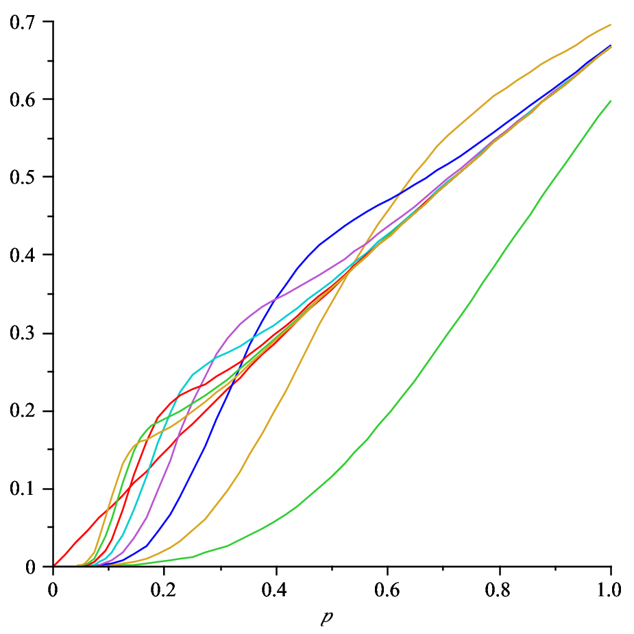
Together with the recursion given for $f_{n}(p):=\operatorname{\mathbb{P}{}}_{{\vec{G}(n,p)}}(a\mathrel{\not\to}s)$ in [2] we will be able compute the covariance for $n$ as a rational function in $p$. Our computations for $n\leq 34$, using Maple, supports our Conjecture 1 that the covariance is always positive, see Figure 1.

For a vertex $v\in V(G)$, let $\overset{\rightarrow}{C}_{v}\subseteq V(G)$ be the (random) set of all vertices $u$ for which there is a directed path from $v$ to $u$. We say that $\overset{\rightarrow}{C}_{v}$ is the out-cluster from $v$. Let analogously the in-cluster, $\overset{\leftarrow}{C}_{v}\subseteq V(G)$ be the (random) set of all vertices $u$ for which there is a directed path from $u$ to $v$. Note that we will use the convention that $v\in\overset{\leftarrow}{C}_{v}\cap\overset{\rightarrow}{C}_{v}$. Let as before $y:=1-p/2$ be the probability that an edge does not exist with a certain direction, and let $q:=1-p$ be the probability that there is no edge at all.

For $n\geq 1$, $s\in{{S}}\subseteq[n]$ and $|{{S}}|=k$ define:

where in particular $d_{p}(1,1)=1$. A recursion to compute $d_{p}(n,k)$ as a polynomial in $p$ was given in [2].

Note that, by symmetry, also $\operatorname{\mathbb{P}{}}_{{\vec{G}(n,p)}}(\overset{\leftarrow}{C}_{s}={{S}})=d_{p}(n,k)$.

It turns out that the following quantity is possible to compute recursively and enables us to compute $h_{n}(p)$. For $n\geq 2$, $t\in{{T}}\subseteq[n]$, $a\in{{A}}\subseteq[n]$ with $|{{T}}|=\tau,|{{A}}|=\alpha$ and $|[n]\setminus({{A}}\cup{{T}})|=r$ define:

where in particular $N_{p}(2,2,2,0)=x$ and $N_{p}(2,1,1,0)=y$.

We will use the variable $j$ for the size of the intersection $|{A}\cap{T}|$. If there is any intersection between ${A}$ and ${T}$ then $a,t\in{A}\cap{T}$, so in particular $j=\alpha+\tau-(n-r)$ can never be 1.

References

• [1] Sven Erick Alm and Svante Linusson, A counter-intuitive correlation in a random tournament, Combin. Probab. Comput. 20 (2011), no 1, 1–9.
• [2] Sven Erick Alm, Svante Janson and Svante Linusson, Correlations for paths in random orientations of G⁡(n,p)G(n,p) and G⁡(n,m)G(n,m), Random Structures and Algorithms 39, No. 4, 486–506 (2011).
• [3] Geoffrey R. Grimmett, Infinite paths in randomly oriented lattices, Random Structures and Algorithms 18, No 3, (2001), 257 – 266.
• [4] Colin McDiarmid, General percolation and random graphs, Adv. in Appl. Probab. 13 (1981), 40–60.
• [5] Svante Linusson, On percolation and the bunkbed conjecture, Combinatorics, Probability and Computing 20 no 01, pp. 103-117 (2011).