Conglomeration of kilometre-sized planetesimals
Abstract
We study the efficiency of forming large bodies, starting from a sea of equal-sized planetesimals. This is likely one of the earlier steps of planet formation and relevant for the formation of the asteroid belt, the Kuiper belt and extra-solar debris disks. Here we consider the case that the seed planetesimals do not collide frequently enough for dynamical collisional to be important (the collisionless limit), using a newly constructed conglomeration code, and by carefully comparing numerical results with analytical scalings. In the absence of collisional cooling, as large bodies grow by accreting small bodies, the velocity dispersion of the small bodies () is increasingly excited. Growth passes from the well-known run-away stage (when is higher than the big bodies’ hill velocity) to the newly discovered trans-hill stage (when and big bodies both grow, but remains at the big bodies’ hill velocity). We find, concurring with the analytical understandings developed in Lithwick [40], as well as previous numerical studies, that a size spectrum results, and that the formation efficiency, defined as mass fraction in bodies much larger than the initial size, is , or at the distance of the Kuiper belt. We argue that this extreme inefficiency invalidates the conventional conglomeration model for the formation of both our Kuiper belt and extra-solar debris disks. New theories, possibly involving direct gravitational collapse, or strong collisional cooling of small planetesimals, are required.
I. Introduction
Large solid bodies, ranging in size from less than a kilometer to thousands of km roam in the outskirts of both the solar and many extrasolar systems. In the case of the solar system, Pluto, Sedna and other large Kuiper belt objects are directly detected [59, 27, 5, 55]; and in the case of extrasolar ones, these bodies are inferred from the dust grains that are produced during their mutual collisions. Even a small amount of dust can intercept enough star light to become detectable as debris disks [1, 69]. Surprisingly, of solar-type stars, even at an age similar to the Sun, harbor dust disks that are brighter than ours by more than three orders of magnitude [43].
How do these large bodies form? Are they an intermediate step in the formation route for planets? Why are they not incorporated into Earth or even Neptune-like planets? Why are many exo-debris disks so bright yet ours so anemic? These are the questions we set out to answer.
The conventional picture for the formation of our own Kuiper belt, [54, 22, 66, 31, 30, 47, 56, hereafter SS11] postulates that it started from Earth masses of primordial rock and ice ( solid mass in the Minimum Mass Solar Nebulae) in kilometre-sized bodies. These bodies grew due to pairwise collisions, but only a fraction of the total mass conglomerated into the large ( km) Kuiper belt bodies we see today. The rest was somehow removed. This extremely low efficiency occurs because, theorists argue, as bodies like Pluto grow, they stir the orderly orbital motion of the small bodies to such an extent that the latter can no longer be accreted quickly into large bodies: Plutos starve themselves.
While the calculations behind this picture appear sound, there are serious issues with applying this theory to realistic systems. In the following, we first discuss why this theory fails to explain the observed extra-solar debris disks, followed by a more detailed discussion on why we believe it fails to explain our own Kuiper belt.
The brightness of Gyrs-old exo-debris disks implies that the total mass contained in their large objects must be times that in our own system [57]. The above mentioned low efficiency then demands that the extra-solar debris disks be formed out of of primordial solids. The total disk mass, if supplemented with the missing hydrogen gas, would then reach of order a solar mass. This is very surprising and, in our view, invalidates the low-efficiency conglomeration model. Moreover, a more top-heavy size distribution is required to explain the brightness evolution of these debris disks [70, 30, 41, 16, 33, e.g.,], than is produced by conglomeration model.
We now turn to discuss the Kuiper belt, with its large sea of literature. With a current mass of in large bodies, the Kuiper belt appears to be well explained by the conglomeration of an initial disk of in kilometre sized bodies. To be compatible with observations, the bulk of these kilometre sized planetesimals had to have been somehow be removed, either by grind-down and blown-away by solar radiation pressure, or by dynamical interactions with giant planets [42, 63]. It is easy to see that the latter removal scenario is not compatible with the existence of the large bodies today. If the dynamical scatterings occurred before the formation of large Kuiper belt objects, these objects would have had to from in a much less massive disk, incompatible with the low efficiency of . In the opposite case, where the scatterings occurred after the formation, large KBOs will be removed as frequently as the small ones, asthe scattering process is mass-insensitive [60, 39]. This would imply a much more massive KBO belt (in large bodies) must have originally formed than is observed today, again requiring a high efficiency for their formation. For example, if scattering removed of the primordial mass, then the large KBOs would have to have been more numerous in the past.
What about removal by radiation pressure? While plausible for the other trans-Neptunian populations, this is clearly not an option for the cold classical Kuiper belt situated at AU. These bodies are likely formed in-situ, as evidenced by their unique colors and dynamically cold orbits [4, 11, 37]. And they are likely formed in a disk that is low in mass: models of Neptune’s migration demands that the massive MMSN disk has to end at AU [63, 20], or else Neptune will continue to plow beyond its current position. Moreover, a massive disk of of kilometer-sized bodies would have disrupted the long period Kuiper belt binaries, which are observed in abundance in the cold classical belt [51, 50].
So in summary, both the extra-solar debris disks and our own Kuiper belt require a formation mechanism that is more efficient than the conventional conglomeration model. One such possibility may be that these large objects are results of direct gravitational collapse within the protoplanetary disk, initiated by, e.g., streaming instability [71, 28] or turbulent concentration [10, 6] This possibility is epitomized in a catchy phrase, ‘Asteroids are born big’, by Morbidelli et al. [44]. Unfortuantely, this scenario has yet to provide reliable predictions for both the efficiency and the size distribution of the objects thus formed.
A second approach is to boost the efficiency by cooling the seed planetesimals, either by gas damping [53, 48, 38, 68], or by inelastic collision between the seeds [19, hereafter GLS]. In a companion paper, we explore the collisional cooling in detail. This is important when planetesimal seeds are so small that their frequent mutual collisions are able to keep their velocity dispersion low. This then guarantees efficient accretion by large bodies, until almost all mass has been converted to large bodies. Such a high-efficiency scenario allows the in situ formation of the cold classical Kuiper belt, as well as the high mass in bright exo-debris disks.
But for the current publication, we restrict ourselves to the conventional case of no collisional cooling. There are three purposes to this paper. One is to document our coagulation code and certify its various components against analytical expectations (§II). This code contains collisional break-down and cooling, but these two effects are unimportant here since we adopt large initial sizes for the planetesimals. Second, we vigorously demonstrate that, in the case of collisionless growth, the formation efficiency is limited to where , the angle subtended by the Solar disc at a distance (§III). In the Kuiper belt region, . Hence only of the initial mass could have been incorporated into large bodies that one observes there today (if growth was nearly collisionless). Equivalently, to form these bodies the initial mass in planetesimals would have had to be , similar to that expected in a MMSN disk extrapolated to the Kuiper belt distance, [64, 23]). Lastly, we compare results from our code against previous work (§V). In particular, 56 have recently proposed a simple explanation for the size distribution of Kuiper belt bodies, in the case of collisionless conglomeration. We examine their claim critically.
This paper should be considered a numerical companion to the recent work by Lithwick [40] where a conglomeration phase called ‘trans-hill growth’ is first discussed. That paper, largely analytical, arrives at similar conclusions as those reached here.
II. The Conglomeration Code: Component testing
We adopt a particle-in-a-box approach [54] to study the interactions of planetesimals and their growth. The range of body sizes we track runs from to .11 1 This is expanded in our next work when we consider grains as small as . Since the total number of particles active in our simulations can exceed , and we typically integrate the system for up to dynamical times, we adopt by necessity a statistical approach where particles with similar properties (mass, eccentricity, inclination, semi-major axis) are grouped into the same bin. We do not yet have the capability of coupling N-body integrators with the statistical code, as was done by Bromley & Kenyon [3], Kenyon & Bromley [30], Glaschke [17]. As such, we cannot accurately capture the evolution at late times, when only a few large bodies dominate the evolution.
II.1. Particles and Bins
A total of six parameters are needed to specify an orbit. We choose the semi-major axis , the eccentricity , the inclination , the argument of periapse , the longitude of the ascending node , and the mean anomaly . Together with mass, each particle should be described by seven parameters. This is computationally prohibitive and approximations are in order. In the following we explain the simplifying assumptions we make in this code.
We adopt a single-value of semi-major axis (AU) for all particles, spread to a width AU. Our single zone approach limits us to study systems where the eccentricities are small (). The particles are assumed to be distributed uniformly in , , and . We set , as is approximately true if random energy is equipartitioned in each dimension [24]. So velocity anisotropy, important when particles are very cold [25, 53], is not properly treated here.
These simplifications allow us to describe particles only by their masses and eccentricities. Following the approach of Wetherill & Stewart [66], particles are first binned by mass. Mass bins are spaced logarithmically, typically with 20 bins per mass decade (i.e., a relative width ). These mass bins may “float” around as evolution proceeds, allowing for more accurate tracking of the mass distribution. Variations of this approach are commonly used in conglomeration codes as they allow for reasonably fast computation times [31, e.g.,]. Each mass bin is assigned a single eccentricity value, which evolves with time. Particle radii are computed by assigned all particles the same bulk density, .
Processes detailed in the following section drive mass and eccentricity evolution and we use a second-order Runge-Kutta integrator to advance the simulation in time. The timestep is set so that no bin has an eccentricity change of more than , and the change in the total number of bodies in a bin is not more than , although is always allowed to be .
There are a few technical subtleties regarding mass evolution. When the mass of a bin strays by more than half a bin spacing from its original value, bodies are promoted to the next highest bin, while the mass of that bin is reset. This is done in a way to conserve the total mass and the total number of particles. As the average mass of a promoted body will not exactly match the average mass in the next higher mass bin, this slightly alters the average mass of the next higher mass bin. Furthermore, for the largest few bodies, their respective zones of dynamical influence do not overlap, and they should not interact with one another. The size of such bodies is called the “isolation mass” (size ) [25, 67, 35] , defined by
| (2) |
We emulate the approach of Kenyon & Luu [31], by pseudo-isolating the biggest bodies so that they do not accrete each other. We also require that bodies larger than to be promoted in integer numbers, to avoid the problem of the runaway growth of a fractional body.
II.2. Dynamical Friction & Viscous Stirring
Mutual gravitational interactions lead towards equipartition of random kinetic energies between bodies. This is called dynamical friction [7]. Additionally, in a keplerian disk, gravitational interactions between bodies converts their orbital energy into random kinetic energy. This is called viscous stirring [54].

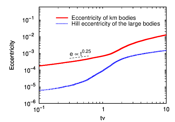
To model dynamical friction and viscous stirring, we adopt the prescription of [46], who provide semi-analytic formulae for the rates at which eccentricity and inclination evolve through gravitational scatterings, calibrated by N-body simulations. But when the mutual velocity of two bodies are below their mutual Hill velocity (sub-hill), we adopt instead the viscous heating prescription in eq. (13) of Collins et al. [9], calibrated by the numerical simulations of Collins & Sari [8].
GLS give explicit formula for the rate of viscous stirring and dynamical friction, depending on whether the velocities are sub- or super-hill (also called shear- or dispersion-dominated). They consider two groups of particles, smaller bodies with size , surface density and velocity dispersion , and large bodies with radius , surface density and velocity dispersion . The two most relevant expressions are viscous stirring of small bodies by the big ones, and dynamical friction of the big bodies by the small bodies. Assuming , these are
| (3) | |||||
| (4) |
Viscous stirring of large bodies by themselves can be found by substituting for in equation 3. As Fig. 1 shows, our adopted prescriptions agree with the above estimates well, when in the above expressions are substituted by . Here, is the Hill velocity of large bodies,
| (5) |
The big body mass with being the bulk density. We set to be the mean density of the Sun, and use to denote the angular size of the Sun, viewed by the bodies, . For the Kuiper belt, .
II.3. Collisions: cooling and cascade
Our conglomeration code includes the collisional process. Although we do not include collisional disruption, and collisional damping is unimportant in this collisionless study, it is essential for our follow-up studies of collisional growth. We document both here for completeness.
In the particle-in-box method, the frequency of collision for a particle is . Here, is the number density of other particles, the cross section for collision, and the relative velocity. The relative velocity between two particles is simply set to be where is as defined in equation (1).
Under our assumption of evenly distributed orbital angles, particles with eccentricity occupy a torus in space that has a volume [see 36, for a detailed derivation],
| (6) |
Their number density is then obtained by where is the particle number. Between two groups of particles with different ’s (, but the same ), their overlapping volume is determined by the group with the smaller (let it be ), and the collision frequency is reduced by a ratio of to take account of the reduced residence time group particles spend inside .
We adopt a three-piece form [21, GLS] for the cross-section for collision between particles of size and ,
| (7) |
We follow GLS and name them super-hill, sub-hill, and super-thin cases. The last case occurs when the velocity dispersion is so small the particles can be regarded as infinitely thin in the vertical direction. These expressions apply when the velocity dispersion is isotropic ().
The outcome of collisions is modelled as changes in mass and eccentricity. We calculate the eccentricity evolution rate for collisions with the GLS order-of-magnitude estimate for this rate,
| (8) |
where is the collisional frequency. Numerically, we obtain a dimensionless coefficient , using Monte-Carlo simulations of equal mass bodies on orbits with the same (, ) and a coefficient of restitution of zero (very inelastic collision).
In terms of mass evolution, collisions can lead to catastrophic destruction, (inelastic) rebound, or conglomeration. Catastrophic collision is defined where the primary body loses of its mass. We specify this to happen if the specific kinetic energy in the impact, , exceeds the disruption threshold [61],
| (9) |
with all numbers in cgs units. This is the scaling for weak aggregates, and may be appropriate for Kuiper belt bodies. For km-sized bodies, . This corresponds to a disruption velocity of , or at AU.
When bodies of size are catastrophically disrupted, we re-distribute their masses to smaller size bins with a number distribution that is power-law in size, for . We typically choose . This distribution results in most of the mass ending up in the largest fragments. And Fig. 2 shows that results do not vary when we vary the value of from to . Furthermore, to imitate the effect of radiative pressure, we remove all mass in size bins below our minimum size (at one micron). In the future, it may be useful to implement the dependence of the largest fragment mass on the impact energy [61].

To verify the collisional mass evolution, we test our code against the standard case of collisional equilibrium for which an analytical solution is known. For a material strength , the collisional cascade will carry a constant mass flux downward in particle size and build up an equilibrium size distribution of [12, 13],
| (10) |
with . The well-known Dohnanyi law is the special case with and hence . In the numerical experiment shown in Fig. 2, we adopt a constant strength of , and initialize the particle size distribution with . Irrespective of the power-law we choose for the debris redistribution, we find that small bodies in the system settle into the expected form and larger bodies gradually enter into collisional equilibrium as time goes on.
If the collision energy is too low to cause destruction, we separate the outcomes into two further categories: rebound or conglomeration. In our code, conglomeration occurs when the relative velocity falls below ten times the mutual escape velocity. This disfavors conglomeration of small bodies: kilometer-sized bodies only accrete each other when at Kuiper belt distances.
When this is not satisfied, the bodies rebound, with an eccentricity damping as described by Eq. (10). In the case of unequal masses, the cooling rate is reduced by . We do not model either cratering collision or sticking by chemical forces. Note that mass loss due to cratering collisions may be the dominant source for the destruction of large bodies [34, 15], and it may be necessary to consider them in realistic models of collisional disruption. Fragmentation can also reduce the effectiveness of planet formation, especially if the fragmenting material can be lost by other means [26, 29] although this primarily concerns growth at larger sizes than we consider here. In the following, we discuss in more detail the accretion process.
II.4. Collisions: accretion
The collisional cross sections in eq. (7) lead to the following rates of accretional growth (GLS), for bodies with size and velocity dispersion , accreting smaller bodies of surface density and velocity dispersion (with )
| (11) |
We confirm that our numerical algorithm does reproduce the above relations. There is a subtlety here. These expressions assume an isotropic velocity dispersion, . However, when stirring is in the sub-hill regime (, eq. 3), inclinations of bodies are excited at a lower rate than their eccentricities, while both quantities are damped by dynamical friction at comparable rates. We then expect these bodies to satisfy and the accretion rate should proceed as the super-thin case (GLS), in which case the accretion rate is for all . In practice, however, stirring is contributed by bodies of various sizes, not just the largest sizes. Short of tracking the inclination evolution, it is difficult to ascertain the accretion geometry. So in this work, we simply assume an isotropic velocity dispersion even though it carries mistakes that may reduce accretion rate by up to . This issue matters only when dealing with accertion among big bodies, which, fortunately, is not significant in the current study.
We perform tests to verify our accretion algorithm. For the following three cases where the accretion cross section between any two bodies is, a) a constant, b) scales as the sum of their masses, , c) scales as the product of their masses, , there exist analytic solutions for the evolution of the size distribution [65]. We integrate these evolutions using our code and compare the numerical outcome against the analytical results (Fig. 3. Our code reproduces the analytic solutions well, except for case c), where the cross section rises steeply with mass, our numerical results reaches the singularity about earlier in time than expected. Other floating mass bin codes hit this singularity later than expected, not earlier [31, 49, e.g.], though the precise disagreement depends on the details of implementation [65].


III. Conglomeration: Results and Analysis


In the remainder of this paper, we present the results of a number of collisionless simulations, in which rebounding and destructive collisions are disabled in the code, but conglomeration still occurs when bodies collide at a speed less than ten times their mutual escape speed. We focus on collisionless simulations in order to compare with previously published results, in which typically small bodies collide only a few times over the course of the simulation. In an upcoming paper, we shall consider the effects of collisional damping and destruction.
We present detailed results from a fiducial simulation in Fig. 4, with Fig. 5 providing diagnostic detail. For ease of comparison, we initalize our planetesimal disk similarly to those in previous works [31, SS11]. Our disk is made up of planetesimals with a surface density of , comparable to the solid value in a MMSN disk. Spread over a radial width of at AU, this corresponds to a total mass of . The bodies ( of them) are initially placed on dynamically cold orbits with .
The growth of the largest bodies is mainly due to accretion of kilometer bodies, at all times. So an important quantity to focus on is eccentricity of the km bodies. The following scalings for the Kuiper belt region will prove useful: , where is the escape speed from a body of size , and . We also discuss two related distributions: the number distribution and the mass distribution. If the number distribution is , then the mass distribution is .
The km bodies have a mean collision frequency
| (12) |
This is the natural timescale in the problem of interest. So from now on, we express time always in unit of .
III.1. Three Growth Stages
The growth can be naturally divided into a few stages.
1. Geometric accretion Initially, stirring is much faster than growth until , and hence the initial growth is dominated by pair-wise conglomeration among equal-sized bodies (size ). Assume collisions occur with geometric cross-section. At time , the average collision probability for each of the km-sized bodies is , but the probability of a single body having experienced collisions is . The size distribution at this point falls off steeply with . The largest body possible at time is determined by , or at a radius of
| (13) |
So at , the largest body has a size of (ignoring gravitational focusing; see below). By this time, km bodies have stirred each other to of their escape velocities (eq. 3), or, , much above of the largest bodies already formed.
2. Rapid Run-away If small bodies are super-hill, the largest bodies experience run-away. They pull away from the rest of the pack while carrying little total mass (left panel of Fig. 4). Eq. (11) indicates that the slowest growth occurs at the smallest size. So once the geometric accretion produces bodies with , the bottle-neck is overcome and very large bodies can be conglomerated within a comparable amount of time.
During this stage of rapid runaway, the small bodies dominate the stirring, and their eccentricities increase very gradually (see Figure 5). The big bodies grow faster than they can stir, and their size spectrum is very steep, . With time, decreases towards unity and we enter the following newly-discovered phase of growth [40].
3. Trans-hill growth (or slow run-away) Rapid run-away ends once the big bodies dominate the stirring. Thereafter, the big bodies’ stirring interferes with their feeding, and the big bodies grow at the same rate as the small bodies’ eccentricities are stirred.
| (14) |
Big body stirring exceeds that of small bodies when
| (15) |
For our simulation, this is satisfied when and , at a time of .
This transition point is affected by the value of , if the initial velocity is such that . If the initial excitation is , for instance, the transition would occur at with again . Lastly, this transition point can be affected by the initial size spectrum of big bodies.
Let us define a class of trans-hill bodies () which always satisfy . These bodies are when the rapid run-away transitions to slow run-away. Following Lithwick [40], we argue that these trans-hill bodies remain effectively the main stirrers in the system, , or equivalently, , in subsequent growth. Hence the name ‘trans-hill’ growth.
To demonstrate this must be true [40, for a more detailed explanation, see], we consider the growth of bodies above and below . Growth of bodies with is in the super-hill (runaway) regime. Their growth rate (eq. 11) can be written as
| (16) |
Since this decreases with decreasing , the size spectrum for is largely frozen.
Growth of bodies with is in the sub-Hill (orderly) regime. The shape of their size spectrum remains invariant with time. Since the initial size spectrum falls steeply beyond , stirring is initially dominated by bodies of size . And this will remain so throughout the trans-hill growth.
As a result of these two considerations, during the trans-hill growth. Equation (15) continues to hold, so the size spectrum extends to larger and larger sizes with , or . This is the value we find in our simulations, and similar results were found by Kenyon & Luu [31], Ormel et al. [47], and 56. An explanation for the slope of the size spectrum, different from our above one, is given in 56. We discuss our different interpretations further in §V.
In our simulations, bodies as large as are formed by . This is consistent with the mass-doubling time for the stirring bodies one obtains from eq. (11), . At this time, large bodies are separated too much to affect each other [66], they are oligarchs [35, see, e.g.]. The appearance of oligarchs effectively terminate the trans-hill stage. However, much of the growth has occurred.
III.2. End of Growth
The efficiency of formation, defined here as the mass fraction in bodies larger than , reaches towards the end of trans-hill growth (Fig. 4). The largest bodies formed are , or Pluto-sized. We argue below that the growth effectively stops when these values are reached. In other words, collisionless conglomeration produces large bodies but at a very low efficiency.
During slow run-away, equation (15) is continuously satisfied, yielding . So the largest size bodies that can form in our simulation, insisting on at least one such body, is . And indeed we observe that evolution practically stalls when . The formation efficiency, defined as the fractional mass accumulated in bodies greater than , is then
| (17) |
and is of order in the Kuiper belt region. In Lithwick [40], we argue that trans-hill growth is typically terminated when a single big body dominates its own feeding zone, i.e., when the biggest bodies become oligarchs [35].
Our statistical code loses some validity once the oligarchic phase commences. A statistical code coupled with N-body dynamics is needed. However, we can project the subsequent growth fairly robustly for the Kuiper belt region, because there is little growth past this point. Neither the big body number nor their spectrum will change much after this.
After trans-hill growth is terminated, small bodies are stirred to super-hill velocites, as until reaches (Fig. 5). With such a hot population of small bodies, accretion by the big bodies proceeds with geometrical cross-section. Yet geometric accretion is far too inefficient to form the observed population of Kuiper belt objects within the Solar system lifetime.22 2 Pluto, for instance, has a geometrical optical depth of . So there is no subsequent accretion to raise the efficiency of big body formation much above . This low formation efficiency is a consequence of our neglect of collisions amongst small bodies. In a forthcoming paper, we show that when collisions are included, the formation efficiency can rise to nearly 100%.
Growth is likely to evolve into the collisional regime. Even if planetesimals start as km-sized, as they are continuously stirred, they approach their destruction speed at (eq. 9). Their mutual collisions beyond this point should be destructive and will produce many small debris. When this occurs, collisional cooling among small planetsimals can no longer be ignored. Growth will then be in the collisional limit.
A minor caveat concerns our assumption of isotropic velocity dispersion for all bodies. For large bodies which stir each other in the sub-hill range, the inclination dispersion may fall much below that of their eccentricities [53, 19]. It is likely that accretion among large bodies could proceed then at a rate greater than that adopted here.
III.3. Simulations with Different Initial Conditions
Our above understanding of the conglomeration process allows us to explain the following dependences when initial conditions in the simulation are altered. In all cases, we find a similar size spectrum to that obtained above. We delay the discussion on the -dependence to §V.2.
- •
initial eccentricity We compare the growth of bodies with initial eccentricities ranging from to , with all other properties held constant. The escape velocity from km bodies is at 45 AU. We find that simulations with initial velocity dispersion smaller than this quickly converge to our standard case; while those with velocity dispersion above this value first undergo orderly growth and produce a more significant mass in intermediate class bodies. In all case, the final efficiency is .
- •
initial surface density We vary the initial surface density of solids from times to times the MMSN values (our standard case being MMSN), with an initial eccentricity of . We observe that the growth time scales inversely with the surface density (Fig. 6). This is because the natural timescale in the problem is the small body collision time (eq. 12). This result has been reported by Kenyon & Luu [31]. We also find that higher mass disks can harbor larger – the final size of the largest body scales roughly as , a result of us insisting that the largest bin has at least one whole body. Lastly, the efficiency of formation only depends logarithmically on the initial .

Figure 6.— Growth of as a functions of time, for disks with different surface densities. The total mass spans from MMSN (bottom-most curve) to , , , and MMSN (top-most curve), with the thick red curve being our fiducial case (Fig. 4). We find the timescale of runaway growth obeys . All growth follow the pattern of a rapid run-away, followed by a slow run-away. 
Figure 7.— Growth of the largest body in simulations with different initial sizes. Initial sizes range from 10 m (the fasest growing) to 100 km (the slowest growing). Bodies grow slowly at first, with the velocity dispersion set by the escape velocity of the initial bodies. Eventually a few bodies run away, when they are sufficiently large. The timescale of runaway increases linearly with starting size. However, the largest bodies that formed are similar in size. - •
initial size We perform a suite of simulations with different starting sizes ranging from m to km. Since the mean collision time (eq. (12)) scales inversely with starting size, and the entire evolution takes place within a few collision times, we expect that a smaller starting size leads to quicker growth. This is observed in Fig. 7 where the growth time scales roughly as yrs.33 3 This is steeper than the relation of found by Kenyon & Luu [31]. We suspect that this may relate to their initial conditions of super-escape velocity dispersions. The size of the largest bodies that form and the size spectrum are comparable in all simulations. More importantly, the efficiency of formation () remains similarly low in all cases.
To summarize, changes in surface density and initial size primarily affect the conglomeration results through their effect on the mean collision frequency (eq. 12). However, neither the size spectrum nor the formation efficiency is much affected by changes in initial conditions.
IV. Comparison against Observed Populations
Here, we contrast the conglomeration results against observations. There are two contexts where this is possible. First, the extra-solar debris disks. The dust brightness of these disks reflect the number densities of parent bodies. As the disks age, the relevant parent bodies have larger and larger sizes. So by studying how the dust luminosities of these disks evolve with time, as an ensemble, it is possible to infer the size spectrum as well as number densities of the parent bodies [57]. This is illustrated in Fig. 8, along with predictions from conglomeration calculations. Starting from a MMSN solid disk (), coagulation of km-bodies leaves most of the primordial mass at the initial sizes, and not enough large bodies are formed. This falls short to explain the brightness of debris disks at advanced ages, by a few orders of magnitudes.

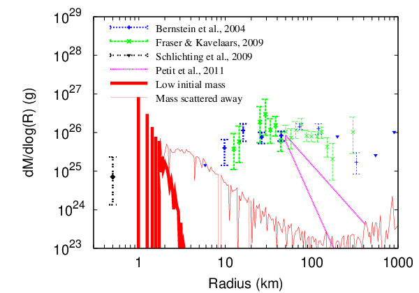
Now we compare our results against observations of Kuiper belt objects (Fig. 9). We have performed two integrations, the first one starting with a low-mass km-sized population (), one that is allowed to exist for the age of the Solar system without destroying the Kuiper belt binaries [51, 50]. The collision time in this case is so long that large bodies cannot be formed, even after 4.5 Gyrs of evolution. The second case is our standard MMSN disk (), which subsequently undergoes a ‘scattering away’ event to make it compatible with the existence of the long period binaries. Although the un-scattered case is capable of producing the observed large Kuiper belt objects, when considering this other constraints, such a scenario is no longer feasible ( also see the introduction).
V. Comparison with Previous Works
V.1. Kenyon & Luu (1998)
We conduct a comparison to the simulations of Kenyon & Luu [31]. We choose this paper for comparison over subsequent ones from the same group because simulations in this paper experiences negligible influence from the gas dynamics and have initial conditions that are the closest to our set-up. They begin with bodies of a single size (we will compare here to their case), with a total mass of in an annulus from to AU and an eccentricity of . This value corresponds to the escape velocity from -sized bodies. So the early accretion (before reaching ) proceeds slowly without the benefit of gravitational focussing. Adopting their initial parameters, our conglomeration code yields size of the largest body at any given time, , as in Figure 10. The growth time in our simulations agree within from those in Kenyon & Luu [31]. We also compare the resulting cumulative size-number distribution, and find it to be in good agreement (Fig. 11). Whatever minor differences that exist may be a result of the different approachs in mass bins, viscous stirring & dynamical friction, cross sections, collisional damping, or any combination thereof. The overall agreement of the two studies demonstrates that the outcome is generic and is not significantly affected by the details of the code.


V.2. 56
While earlier works have performed exhaustive studies of the conglomeration process, 56 is the first to present a simple analytical argument for the numerical results and is thus the most relevant work for comparison. Here, we critically examine their argument.
56 aims to explain the spectrum, obtained by all works, as a result of big bodies growing by equally accreting small bodies and other big bodies. They assume that the largest bodies grow both by accreting each other and by accreting small bodies, at equal rates (‘equal accretion’). This assumption, which we examine here, enables them to derive a mass spectrum of , with a (constant) efficiency of large body formation of . These claims appear to be backed up by their simple yet elegant numerical experiments.
However, it is unclear why, on physical grounds, equal accretion should occur.44 4 Ormel et al. [47] claimed to observe equal accretion in their numerical simulation. However, fragmentation included in their study has reduced the mass in, and hence accretion from, small bodies. Instead, we have shown that the spectrum arises due to the fact that the largest bodies at any given time are trans-hill relative to the small bodies. We present a physical argument why this is naturally achieved (§III.1). To test whether equal accretion or trans-hill accretion is the important physics driving the size spectrum, in our code, we disallow big bodies from accreting one another: they are forbidden from accreting bodies more than 10% of their masses. We begin the simulation with a narrow spectrum (as opposed to a delta-function, as our new formulation will otherwise stall any growth) of initial bodies. We recover a size spectrum, despite the absence of equal accretion (Fig. 12).

A second test to judge between the two interpretations is possible. Our expected efficiency of growth scales as , while SS11 predicts an efficiency of . In Figs. 13 and 14, we compare simulations conducted at different semimajor axis, and hence different , plotted before the onset of oligarchy. To avoid oligarchic effects, collisional cooling, and contributions from intermediate-sized bodies, the simulations are started with different initial sizes that are proportional to . It appears that the numbers of large bodies scale better with than with . The numerically obtained efficiency is . This appears to support the interpretation of trans-hill accretion. Interestingly, during trans-hill accretion, accretion of small bodies and large bodies occurs at a fixed ratio [40, see Section 5.1 of]. But it is an effect rather than a cause.


VI. Conclusions
In this contribution, we focus on the efficiency of forming large bodies by conglomeration, starting from a sea of small planetesimals that are not cooled by frequent collisions. We find, concuring with previous studies, that the formation efficiency is , or at the distance of the Kuiper belt.
We obtain this result numerically by constructing a conglomeration code that incorporates physical processes such as viscous stirring, dynamical friction and accretion. This code also has the capability of dealing with catastrophic disruption and collisional damping. But in the current study with initial size of km, collisional cooling is not relevant and we do not allow bodies to break down to smaller particles.
We also derive the formation efficiency analytically [40]. We find that in collisionless environments, growth passes through several stages, but naturally transitions to the most critical stage, which we term ’trans-hill’ growth Growth is a run-away process when small bodies are super-hill and an orderly process when small bodies are sub-hill. Consequently, the biggest body at any given time sits at trans-hill, or . The fact that the system is driven to trans-hill growth is the key for why the size spectrum is with , and why the formation efficiency is .
To be confident of our numerical procedure, we have tested individual components in the code against the order-of-magnitude formulae in GLS. We have also performed detailed comparisons with previous simulations. These include 56 and [31]. All previous works yield a similarly low formation efficiency, and a similar size spectrum () as we obtain here. But some detailed differences exist. Comparison against [31] show that we reproduce their overall results, but with differences in both time-scales and size distributions. 56 postulated that equal accretion drives the size spectrum, and low efficiency. We, by explicitly forbidding accretion among big bodies, show that the correct physical interpretation is likely not related to equal accretion, but to trans-hill accretion. This is also supported by the scaling of formation efficiency with distance to the central star.
In the collisionless limit, trans-hill growth ends when the largest bodies become oligarchs, each responsible for stirring their own food. Subsequent accretion in this phase does not increase significantly the formation efficiency, at least in the Kuiper belt, due to the impossibly long accretion timescale for Pluto-type objects.
Surface densities in large bodies in the Kuiper belt have been measured to be of that of the MMSN, and the largest bodies are in size. These have traditionally been viewed as successes for the collisionless coagulation theory. However, recent discoveries of bright extra-solar debris disks call this into question. Their dust luminosities reveal that they likely harbor large bodies that are a factor of times greater in number than that in our Kuiper belt [57], comparable to the total mass in a MMSN solid disk in these outer regions. This conflicts with the low formation efficiency, which is the generic outcome of collisionless conglomeration. So even if the size spectrum of KBOs may be explained by the collisionless process, doubts on which still linger, the low efficiency of collisionless conglomeration precludes it from being the process which forms debris disks, including the Kuiper belt. In our simulations, km-size bodies reach such high velocity dispersion towards the end, that their mutual encounter should cause fragmentation into smaller particles. This is also observed in Kenyon & Luu [32]. So even if planetesimals start as large as , collisional cooling may set in at some stage. An evolutionary path that is qualitatively different from that described here may ensue.
To resolve the issue of long formation timescale for Uranus and Neptune, Goldreich et al. [18] have proposed that conglomeration proceeds in a collisional environment, where small bodies are so small they are cooled by frequent collisions. In future works [58], we follow this path and demonstrate that collisional conglomeration would also be able to raise the efficiency of formation to of order unity, thereby explaining, within one paradigm, the formation of the Kuiper belt and the extra-solar debris disks.
References
- [1] Aumann, H. H., Beichman, C. A., Gillett, F. C., de Jong, T., Houck, J. R., Low, F. J., Neugebauer, G., Walker, R. G., & Wesselius, P. R. 1984, ApJL, 278, L23
- [2] Bernstein, G. M., Trilling, D. E., Allen, R. L., Brown, M. E., Holman, M., & Malhotra, R. 2004, AJ, 128, 1364
- [3] Bromley, B. C. & Kenyon, S. J. 2006, AJ, 131, 2737
- [4] Brown, M. E., Schaller, E. L., & Fraser, W. C. 2011, ApJ, 739, L60
- [5] Brown, M. E., Trujillo, C. A., & Rabinowitz, D. L. 2005, ApJ, 635, L97
- [6] Chambers, J. E. 2010, Icarus, 208, 505
- [7] Chandrasekhar, S. 1943, ApJ, 97, 255
- [8] Collins, B. F. & Sari, R. 2006, AJ, 132, 1316
- [9] Collins, B. F., Schlichting, H. E., & Sari, R. 2007, AJ, 133, 2389
- [10] Cuzzi, J. N., Hogan, R. C., & Shariff, K. 2008, ApJ, 687, 1432
- [11] Dawson, R. I. & Murray-Clay, R. 2012, ApJ, 750, 43
- [12] Dohnanyi, J. W. 1969, J. Geophys. Res., 74, 2531
- [13] Durda, D. D. & Dermott, S. F. 1997, Icarus, 130, 140
- [14] Fraser, W. C., Brown, M. E., & Schwamb, M. E. 2010, Icarus, 210, 944
- [15] Gáspár, A., Psaltis, D., Özel, F., Rieke, G. H., & Cooney, A. 2012, ApJ, 749, 14
- [16] Gáspár, A., Rieke, G. H., & Balog, Z. 2013, ApJ, 768, 25
- [17] Glaschke, P. 2006, PhD thesis, PhD Thesis, Combined Faculties for the Natural Sciences and for Mathematics of the University of Heidelberg, Germany. XIV+134 pp. (2006)
- [18] Goldreich, P., Lithwick, Y., & Sari, R. 2004a, ApJ, 614, 497
- [19] —. 2004b, ARA&A, 42, 549
- [20] Gomes, R. S., Morbidelli, A., & Levison, H. F. 2004, Icarus, 170, 492
- [21] Greenberg, R., Bottke, W. F., Carusi, A., & Valsecchi, G. B. 1991, Icarus, 94, 98
- [22] Greenberg, R., Hartmann, W. K., Chapman, C. R., & Wacker, J. F. 1978, Icarus, 35, 1
- [23] Hayashi, C. 1981, Progress of Theoretical Physics Supplement, 70, 35
- [24] Hornung, P., Pellat, R., & Barge, P. 1985, Icarus, 64, 295
- [25] Ida, S. & Makino, J. 1992, Icarus, 96, 107
- [26] Inaba, S., Wetherill, G. W., & Ikoma, M. 2003, Icarus, 166, 46
- [27] Jewitt, D. & Luu, J. 1993, Nature, 362, 730
- [28] Johansen, A., Oishi, J. S., Low, M.-M. M., Klahr, H., Henning, T., & Youdin, A. 2007, Nature, 448, 1022
- [29] Kenyon, S. J. & Bromley, B. C. 2004, AJ, 127, 513
- [30] —. 2008, ApJS, 179, 451
- [31] Kenyon, S. J. & Luu, J. X. 1998, AJ, 115, 2136
- [32] —. 1999, AJ, 118, 1101
- [33] Kobayashi, H. & Löhne, T. 2014, MNRAS, 442, 3266
- [34] Kobayashi, H. & Tanaka, H. 2010, Icarus, 206, 735
- [35] Kokubo, E. & Ida, S. 1998, Icarus, 131, 171
- [36] Krivov, A. V., Sremčević, M., & Spahn, F. 2005, Icarus, 174, 105
- [37] Lacerda, P., Fornasier, S., Lellouch, E., Kiss, C., Vilenius, E., Santos-Sanz, P., Rengel, M., Müller, T., Stansberry, J., Duffard, R., Delsanti, A., & Guilbert-Lepoutre, A. 2014, ApJ, 793, L2
- [38] Lambrechts, M. & Johansen, A. 2012, A&A, 544, A32
- [39] Levison, H. F., Morbidelli, A., Vanlaerhoven, C., Gomes, R., & Tsiganis, K. 2008, Icarus, 196, 258
- [40] Lithwick, Y. 2014, ApJ, 780, 22
- [41] Löhne, T., Krivov, A. V., & Rodmann, J. 2008, ApJ, 673, 1123
- [42] Malhotra, R. 1995, AJ, 110, 420
- [43] Meyer, M. R., Backman, D. E., Weinberger, A. J., & Wyatt, M. C. 2007, in Protostars and Planets V, ed. B. Reipurth, D. Jewitt, & K. Keil, 573–588
- [44] Morbidelli, A., Bottke, W. F., Nesvorný, D., & Levison, H. F. 2009, Icarus, 204, 558
- [45] Nishida, S. 1983, Progress of Theoretical Physics, 70, 93
- [46] Ohtsuki, K., Stewart, G. R., & Ida, S. 2002, Icarus, 155, 436
- [47] Ormel, C. W., Dullemond, C. P., & Spaans, M. 2010, Icarus, 210, 507
- [48] Ormel, C. W. & Klahr, H. H. 2010, A&A, 520, A43
- [49] Ormel, C. W. & Spaans, M. 2008, ApJ, 684, 1291
- [50] Parker, A. H. & Kavelaars, J. J. 2012, ApJ, 744, 139
- [51] Parker, A. H., Kavelaars, J. J., Petit, J.-M., Jones, L., Gladman, B., & Parker, J. 2011, ApJ, 743, 1
- [52] Petit, J.-M., Kavelaars, J. J., Gladman, B. J., Jones, R. L., Parker, J. W., Van Laerhoven, C., Nicholson, P., Mars, G., Rousselot, P., Mousis, O., Marsden, B., Bieryla, A., Taylor, M., Ashby, M. L. N., Benavidez, P., Campo Bagatin, A., & Bernabeu, G. 2011, AJ, 142, 131
- [53] Rafikov, R. R. 2003, AJ, 126, 2529
- [54] Safronov, V. S. 1969, Evoliutsiia doplanetnogo oblaka., ed. Safronov, V. S.
- [55] Schlichting, H. E., Ofek, E. O., Wenz, M., Sari, R., Gal-Yam, A., Livio, M., Nelan, E., & Zucker, S. 2009, Nature, 462, 895
- [56] Schlichting, H. E. & Sari, R. 2011, ApJ, 728, 68
- [57] Shannon, A. & Wu, Y. 2011, ApJ, 739, 36
- [58] Shannon, A., Wu, Y., & Lithwick, Y. 2015, In Preparation
- [59] Slipher, V. M. & Tombaugh, C. W. 1930, The Science News-Letter, 17, 179
- [60] Stern, S. A. 1991, Icarus, 90, 271
- [61] Stewart, S. T. & Leinhardt, Z. M. 2009, ApJ, 691, L133
- [62] Thébault, P., Augereau, J. C., & Beust, H. 2003, A&A, 408, 775
- [63] Thommes, E. W., Duncan, M. J., & Levison, H. F. 1999, Nature, 402, 635
- [64] Weidenschilling, S. J. 1977, Ap&SS, 51, 153
- [65] Wetherill, G. W. 1990, Icarus, 88, 336
- [66] Wetherill, G. W. & Stewart, G. R. 1989, Icarus, 77, 330
- [67] —. 1993, Icarus, 106, 190
- [68] Windmark, F., Birnstiel, T., Güttler, C., Blum, J., Dullemond, C. P., & Henning, T. 2012, A&A, 540, A73
- [69] Wyatt, M. C. 2008, ARA&A, 46, 339
- [70] Wyatt, M. C., Smith, R., Su, K. Y. L., Rieke, G. H., Greaves, J. S., Beichman, C. A., & Bryden, G. 2007, ApJ, 663, 365
- [71] Youdin, A. N. & Goodman, J. 2005, ApJ, 620, 459