Localized Features in Non-Gaussianity from Heavy Physics

First, we briefly review the model presented in Ref. [43]. We consider a model with a heavy scalar field with mass $m\gg H$, $\chi(\equiv\phi^{(2)})$, which derivatively couples to the inflaton field, $\phi(\equiv\phi^{(1)})$, as

	$\displaystyle S_{m}$	$\displaystyle\equiv-\int\mathrm{d}x^{4}\sqrt{-g}P(X^{IJ},\phi^{K}),\qquad(I,J,K=1,2)$		(1)
		$\displaystyle=-\int\mathrm{d}x^{4}\sqrt{-g}\left[\frac{1}{2}(\partial\phi)^{2}+V(\phi)+\frac{1}{2}(\partial\chi)^{2}+\frac{m^{2}}{2}\chi^{2}+K_{n}+K_{d}+{\cal O}\left(X\phi^{2}/\Lambda_{n}^{2},X^{3}/\Lambda_{d}^{8}\right)\right],$		(2)

with $X^{IJ}\equiv-\partial_{\mu}\phi^{I}\partial^{\mu}\phi^{J}/2$. Here, we have assumed that the derivative couplings at the leading order are given by,

$\displaystyle K_{n}$

$\displaystyle\equiv\frac{\lambda_{n}}{2\Lambda_{n}}\chi(\partial\phi)^{2},$

(3)

and

$\displaystyle K_{d}$

$\displaystyle\equiv\frac{\lambda_{d1}}{4\Lambda_{d}^{4}}(\partial\chi)^{2}(\partial\phi)^{2}+\frac{\lambda_{d2}}{4\Lambda_{d}^{4}}(\partial\chi\cdot\partial\phi)^{2},$

(4)

with the dimensional parameters $\Lambda_{n},\Lambda_{d}$ and the dimensionless parameters $\lambda_{n},\lambda_{di}~(i=1,2)$. The derivative couplings in Eq. (2) generally appear in the action from the effective-field-thoery point of view [51, 52] . The derivative couplings $K_{n}$ and $K_{d}$ provide the most general couplings between the inflaton field and the heavy scalar field at the leading order in $1/\Lambda_{n}$ and $1/\Lambda_{d}$ in a model with the parity symmetry, $\phi\to-\phi$, and the shift symmetry, $\phi\to\phi+c$. The approximate shift symmetry is usually assumed to ensure the flatness of the inflaton potential. In addition, we have assumed the parity symmetry to forbid the kinetic mixing, which obscures the difference between the light and heavy fields. Thus, we first focus on the couplings $K_{n}$ and $K_{d}$, though brief comments are presented in §3.4 on expected features in the bispectrum when a symmetry-violating interaction becomes relevant. In general, higher-order terms in $\Lambda_{n}$ and $\Lambda_{d}$ are also expected to appear. To ensure that contributions from these terms can be treated perturbatively, we assume here that the background fields satisfy the following conditions,

$$\chi\ll\Lambda_{n},\quad\dot{\phi},~\dot{\chi}\ll\Lambda_{d}^{2}.$$

(5)

We have also suppressed the terms $(\partial\phi)^{4}$ and $(\partial\chi)^{4}$ in Eq. (2), because they have little effects on our analysis for the background evolution and the power spectrum. The higher-order terms and the self interaction $(\partial\phi)^{4}$ can be important for the bispectrum. Features in the bispectrum induced by these interactions are discussed in §3.4. We can also find many specific models which have the couplings $K_{n}$ and $K_{d}$, such as DBI inflation [53]. In these cases, the conditions (5) are not mandatory.

Since $\chi$ can generally decay into other particles, we assume that $\chi$ decays with a rate $\Gamma$, which satisfies $H\ll\Gamma\ll m$. To ensure the slow-roll inflation, we further make two assumptions. First, the inflaton potential is sufficiently flat,

$\displaystyle\epsilon_{V}\ll 1,~|\eta_{V}|\ll 1,$

(6)

where

$$\epsilon_{V}\equiv\frac{M_{p}^{2}}{2}\left(\frac{V^{\prime}}{V}\right)^{2},\quad\eta_{V}\equiv M_{p}^{2}\frac{V^{\prime\prime}}{V},$$

(7)

are the slow-roll parameters. Here, $M_{p}=2.4\times 10^{18}~\mathrm{GeV}$ is the reduced Planck mass. Second, the heavy scalar field $\chi$ is subdominant,

$\displaystyle f_{\chi}\ll 1,$

(8)

where

$$f_{\chi}\equiv\frac{\rho_{\chi}}{\rho}\simeq\frac{\dot{\chi}^{2}+m^{2}\chi^{2}}{6M_{p}^{2}H^{2}},$$

(9)

is the fraction of its energy density to the total one.

Provided that the conditions (5), (6), and (8) are satisfied, the background evolution of the inflation field is given by the slow-roll solution,

$\displaystyle\pi_{\phi}(t)\simeq-\frac{V^{\prime}}{3H},$

(10)

where $\pi_{\phi}$ is the conjugate momentum for the inflaton field,

$\displaystyle\pi_{\phi}\equiv\hat{z}_{\phi}^{2}\dot{\phi},$

(11)

with

$\displaystyle z_{\phi}^{2}\equiv a^{3}\left[1+\lambda_{n}\frac{\chi}{\Lambda_{n}}+\left(\lambda_{d1}+\lambda_{d2}\right)\frac{\dot{\chi}^{2}}{2\Lambda_{d}^{4}}\right],$

(12)

and $\hat{z}_{\phi}^{2}\equiv z_{\phi}^{2}/a^{3}$. The heavy scalar field oscillates with a frequency of the mass scale $m$,

$\displaystyle\chi(t)\simeq\chi_{0}e^{-\Gamma t}\cos(mt)\theta(t),$

(13)

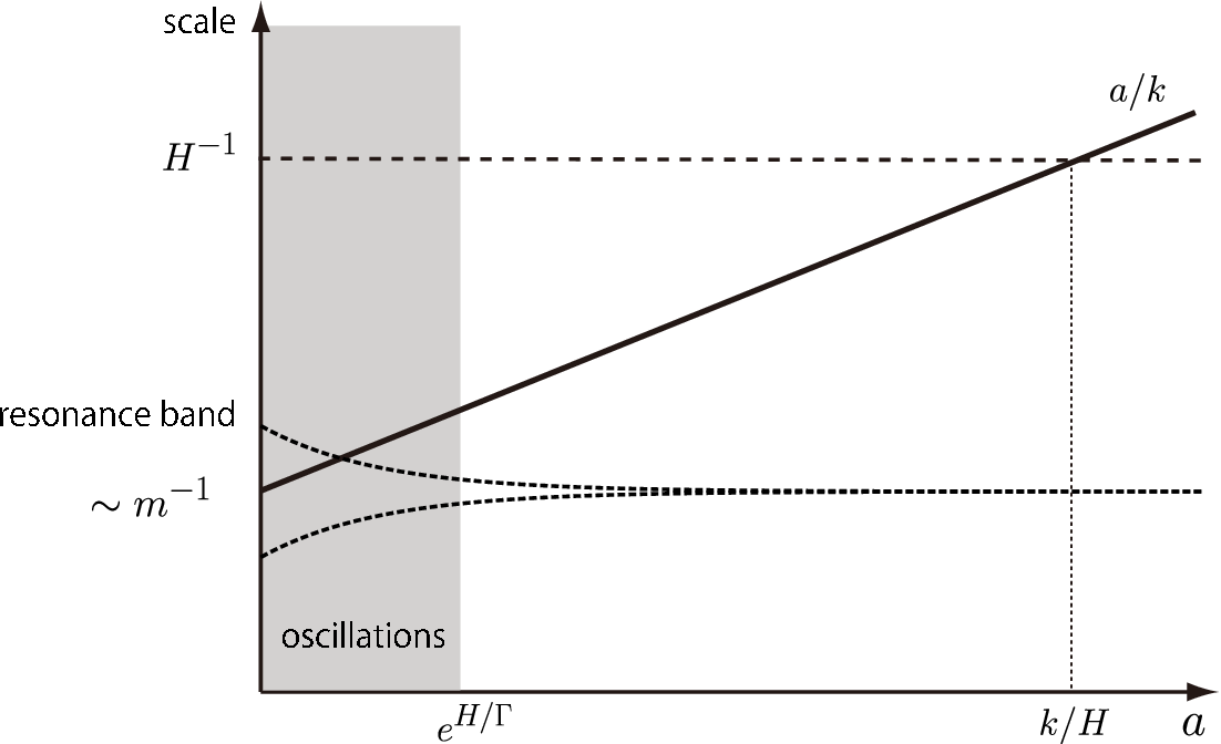
with $\theta(t)$ being the Heaviside function, where we have assumed that the oscillation is excited instantaneously at $t=0$. The fluctuations are enhanced through a resonance with the background oscillation of the heavy scalar field (13). We showed the basic picture of the resonant enhancement in Fig. 1.

For a later convenience, we introduce parameters which represent the magnitude of the derivative couplings,

	$\displaystyle q_{n}$	$\displaystyle\equiv\lambda_{n}\frac{\chi_{0}}{\Lambda_{n}},$		(14)
	$\displaystyle q_{d1}$	$\displaystyle\equiv\lambda_{d1}\frac{m^{2}\chi_{0}^{2}}{2\Lambda_{d}^{4}},\quad q_{d2}\equiv\lambda_{d2}\frac{m^{2}\chi^{2}_{0}}{2\Lambda_{d}^{4}},$		(15)

which are related to the $q$-parameters introduced in Ref. [43]. We will also use $q$ to represent the order of the $q$-parameters above. Note that the $q$-parameters are less than unity under the conditions (5). They can be expressed in terms of the energy fraction of the heavy scalar field, $f_{\chi}$, as

$\displaystyle q_{n}\simeq\sqrt{2}\lambda_{n}\left(\frac{E_{\rm inf}}{m}\right)\left(\frac{E_{\rm inf}}{\Lambda_{n}}\right)f_{\chi,t=0}^{\frac{1}{2}},$

(16)

for the couplings $K_{n}$ and

$\displaystyle q_{d1}\simeq\lambda_{d1}\left(\frac{E_{\rm inf}}{\Lambda_{d}}\right)^{4}f_{\chi,t=0},\quad q_{d2}\simeq\lambda_{d2}\left(\frac{E_{\rm inf}}{\Lambda_{d}}\right)^{4}f_{\chi,t=0},$

(17)

for the couplings $K_{d}$ , where $E_{\rm inf}$ is the energy scale of the inflation, $E_{\rm inf}\equiv(3M_{p}^{2}H^{2})^{\frac{1}{4}}\simeq V^{\frac{1}{4}}$.

Before investigating the features in the bispectrum, we first estimate the effect of the resonance on the power spectrum. To obtain an analytic expression, here, we use the perturbative method assuming that the $q$-parameters are sufficiently small.

To eliminate the gauge degrees of freedom in the metric fluctuations, we use the flat gauge, where the spatial metric becomes $a^{2}\delta_{ij}$. In this gauge, we can make some simplifications in estimating the power spectrum. First, the metric fluctuations can be neglected because the resonance takes place deep in the horizon. Moreover, we can also neglect the fluctuations in the heavy scalar field, $\delta\chi$. This is because $\delta\chi$ oscillates with a frequency $\omega>m$ and therefore does not satisfy the resonance condition. In addition, the mass term suppresses the amplitude of $\delta\chi$ at $k/a\sim m$ compared with that of the inflaton field.

Neglecting the fluctuations in the metric and the heavy scalar field, the second-order action for the fluctuations in the inflaton field, $\varphi$, can be written as,

$\displaystyle S_{2}\simeq\int\mathrm{d}t\mathrm{d}^{3}x~\frac{z_{\phi}^{2}}{2}\left[\dot{\varphi}^{2}-c_{s}^{2}(\nabla\varphi)^{2}/a^{2}\right],$

(18)

where

$\displaystyle c_{s}^{2}=1-\frac{\lambda_{d2}\dot{\chi}^{2}}{2\Lambda_{d}^{4}}+O\left(\frac{\dot{\chi}^{4}}{\Lambda_{d}^{8}}\right),$

(19)

is the speed of sound for the fluctuations in the inflaton field. Note that we can neglect terms like $\dot{\phi}^{2}/\Lambda_{d}^{4}$ in the action (18), which could be induced by the self interaction $(\partial\phi)^{4}/\Lambda_{d}^{4}$, because they are higher order in the $q$-parameters.

Introducing the canonically normalized variable $v\equiv z_{\phi}\varphi$, the action (18) can be rewritten as,

$\displaystyle S_{2}=\int\mathrm{d}t\mathrm{d}^{3}x~\frac{1}{2}\left[\dot{v}^{2}-\left(\frac{c_{s}^{2}\nabla^{2}}{a^{2}}-\frac{\ddot{z}_{\phi}}{z_{\phi}}\right)v^{2}\right],$

(20)

and then the full Hamiltonian as,

$\displaystyle H^{(2)}=\int\mathrm{d}^{3}x~\frac{1}{2}\left[\dot{v}^{2}+\left(\frac{c_{s}^{2}\nabla^{2}}{a^{2}}-\frac{\ddot{z}_{\phi}}{z_{\phi}}\right)v^{2}\right].$

(21)

Substituting the background solution (13), the quantities $c_{s}^{2}$ and $\ddot{z}_{\phi}/z_{\phi}$ can be estimated as,

	$\displaystyle c_{s}^{2}$	$\displaystyle\simeq 1+\frac{q_{d2}}{2}e^{-2\Gamma t}\cos(2mt),$		(22)
	$\displaystyle\frac{\ddot{z}_{\phi}}{z_{\phi}}$	$\displaystyle\simeq m^{2}\left[q_{n}e^{-\Gamma t}\cos(mt)+(q_{d1}+q_{d2})e^{-2\Gamma t}\cos(2mt)+O\left(\frac{H}{m}\right)\right].$		(23)

In the following analysis, we neglect the ${\cal O}(H/m)$ terms in Eq. (23) assuming that $q$ is larger than $H/m$. Taking the free Hamiltonian as the terms independent of the derivative couplings in Eq. (21), the interaction Hamiltonian is given by, ¹¹ 1 Note that infinitely many terms would appear in the interaction Hamiltonian if we define the free Hamiltonian as terms independent of the derivative couplings without introducing the canonically normalized variable $v$.

$\displaystyle H_{I}^{(2)}\equiv\frac{m^{2}}{2(2\pi)^{3}}\int\mathrm{d}^{3}k~C_{k}^{(2)}v_{{\bf k}}v_{\bf-k},$

(24)

where we have moved to Fourier space,

$\displaystyle v(x)=\frac{1}{(2\pi)^{3}}\int{\rm d}^{3}k~v_{\bf k}e^{i{\bf k}\cdot{\bf x}}.$

(25)

Here, the coefficient $C_{k}^{(2)}$ is given in terms of the $q$-parameters as,

$\displaystyle C_{k}^{(2)}\equiv C_{k}^{(2;n)}e^{-\Gamma t}\cos(mt)+C^{(2;d)}e^{-2\Gamma t}\cos(2mt),$

(26)

where

	$\displaystyle C_{k}^{(2;n)}$	$\displaystyle\equiv-q_{n},$		(27)
	$\displaystyle C_{k}^{(2;d)}$	$\displaystyle\equiv q_{d2}\left[\frac{1}{2}\left(\frac{k}{am}\right)^{2}-1\right]-q_{d1}.$		(28)

Hence, using the in-in formalism, the correction to the power spectrum can be estimated as,

$\displaystyle\Delta\langle\varphi_{\bf k}(t)\varphi_{\bf k^{\prime}}(t)\rangle$

$\displaystyle\simeq i\int_{0}^{t}{\rm d}t^{\prime}~\langle[H_{I}^{(2)}(t^{\prime}),\varphi_{\bf k}(t)\varphi_{\bf k^{\prime}}(t)]\rangle,$

(29)

at the leading order in the $q$-parameters, where the fields in LHS are operators in the Heisenberg picture while, in RHS, they represent operators in the interaction picture. For brevity, we denote them in the same way since it will be clear which they represent from the context.

In terms of the dimensionless power spectrum, ${\cal P}_{\varphi}$, defined through,

$\displaystyle\langle\varphi_{{\bf k}}(t)\varphi_{{\bf k}^{\prime}}(t)\rangle\equiv(2\pi)^{3}\delta^{3}({\bf k+k^{\prime}})\frac{2\pi^{2}{\cal P}_{\varphi}}{k^{3}},$

(30)

the correction is expressed as,

$\displaystyle\Delta{\cal P}_{\varphi}(k)/{\cal P}_{\varphi}=I_{k}^{(2)},$

(31)

where

$\displaystyle I_{k}^{(2)}\equiv-2m^{2}{\rm Re}\left[i\int_{0}^{t}{\rm d}t^{\prime}~C_{k}^{(2)}u_{k}(t^{\prime})^{2}\right].$

(32)

Here, the estimation time $t$ should be taken sufficiently after the decay of the oscillation. The function $u_{k}$ is the mode function for $v_{{\bf k}}$, which is defined through,

$\displaystyle v_{\bf k}(t)=u_{k}(t)a_{{\bf k}}+u_{k}^{\ast}(t){a_{-{\bf k}}}^{\dagger},$

(33)

for the creation/annihilation operators. Though the state could be excited depending on the excitation mechanism of the oscillation, we simply assume that the state was in the vacuum state at the excitation of the oscillation. Even if the state was excited, the resonance is not spoiled except for some specific excited states. Assuming that the state is not excited, the mode function is provided by,

$\displaystyle u_{k}(t)=\sqrt{\frac{a}{2k}}\left(1-\frac{i}{k\tau}\right)e^{-ik\tau},$

(34)

where $\tau$ is the conformal time. Because the resonance occurs deep in the horizon, we can approximate the mode functions in the integral (32) as,

$\displaystyle u_{k}(t)\simeq\sqrt{\frac{a}{2k}}e^{-ik\tau}.$

(35)

Hence, $I_{k}^{(2)}$ can be approximated as,

$\displaystyle I_{k}^{(2)}\simeq-\int_{0}^{z}{\rm d}z^{\prime}\left(\frac{k}{am}\right)^{-1}C_{k}^{(2)}\sin(2k\tau^{\prime}),\quad(z\equiv mt).$

(36)

The resonance occurs between the factor $\sin(2k\tau^{\prime})$ and the oscillatory components, $\cos(mt^{\prime})$ and $\cos(2mt^{\prime})$, in $C_{k}^{(2)}$ (see Eq. (26)). If the negative energy mode exists, it would introduce an additional oscillatory component in Eq. (36) with a constant phase shift. However, this additional component does not spoil the resonance unless the amplitude of the negative energy mode and the phase shift have specific values for the scales of the resonance.

Here, we evaluate $I^{(2)}_{k}$ for the couplings $K_{n}$. Replacing the parameters $(q_{n},m/2,\Gamma/2)$ by $(q_{d},m,\Gamma)$, we can obtain a similar result for the couplings $K_{d}$. Using the product-to-sum identities for the trigonometric functions, we have two oscillatory functions in Eq. (36). The integration has a resonant contribution from one of the two in the interval around the stationary point of the phase function, $\theta^{(2;n)}\equiv mt-2k\tau$. Taking the derivative of the phase function $\theta^{(2;n)}$, we can find that the resonance occurs at time $t_{\ast}$ where,

$\displaystyle\frac{k}{a(t_{\ast})}=\frac{m}{2}.$

(37)

Hence, the resonance occurs $\Delta N\equiv\ln(m/2H)$ e-folds before the horizon crossing of the modes. Solving the above equation, the value of $z$ at the resonance is estimated to be

$\displaystyle z_{\ast}\simeq\frac{m}{H}\ln\left(\frac{2k}{a_{0}m}\right),$

(38)

where $a_{0}$ is the scale factor at the onset of the oscillation. Then, the integral can be evaluated as, ²² 2 Note that we have used $2k$ for the argument of $I^{(n)}_{k}$ for later convenience. The factor $2k$ in Eq. (40) corresponds to $k+k^{\prime}$ if we don’t take into account the delta function in Eq. (30). Similarly, the scaling function $I^{(n)}_{K}$ with $K=k_{1}+k_{2}+k_{3}$ appears for the bispectrum.

$\displaystyle I_{k}^{(2)}\simeq C_{k,\ast}^{(2;n)}{\rm Im}I^{(n)}_{2k},$

(39)

where

$\displaystyle I^{(n)}_{2k}\equiv\int_{0}^{z}{\rm d}z^{\prime}e^{-\frac{\Gamma}{m}z^{\prime}+i(z^{\prime}-2k\tau^{\prime})},$

(40)

and $C_{k,\ast}^{(2;n)}$ is the coefficient function (27) at the resonance, $t=t_{\ast}$. The duration of the resonance can be roughly estimated by $\Delta z\equiv m/\sqrt{\ddot{\theta}}$, which is given by

$\displaystyle\Delta z^{(2;n)}$

$\displaystyle=\sqrt{m/H},$

(41)

for the couplings $K_{n}$. Approximating the oscillating factor $e^{i(z^{\prime}-2k\tau^{\prime})}$ in Eq. (40) by a top-hat function, then, we can roughly estimate the contribution to $I^{(n)}_{2k}$ from the resonance through the couplings $K_{n}$ as,

	$\displaystyle I_{2k}^{(n)}$	$\displaystyle\simeq C_{k,\ast}^{(2;n)}\sin\theta^{(2;n)}_{\ast}\int_{\max(0,z_{\ast}-\sqrt{\frac{m}{H}})}^{\max(0,z_{\ast}+\sqrt{\frac{m}{H}})}{\rm d}z^{\prime}~e^{-\frac{\Gamma}{m}z^{\prime}}$		(42)
		$\displaystyle\equiv C_{k,\ast}^{(2;n)}\sin\theta^{(2;n)}_{\ast}I_{2k,\text{approx}}^{(n)}$		(43)
		$\displaystyle={\displaystyle\begin{cases}0&\left(\ln\left(\frac{2k}{a_{0}m}\right)<-\sqrt{\frac{H}{m}}\right),\\ -\frac{m}{\Gamma}\left[1-\left(\frac{2k}{a_{0}m}\right)^{-\frac{\Gamma}{H}}e^{-\frac{\Gamma}{\sqrt{Hm}}}\right]\sin\theta^{(2;n)}_{\ast}q_{n}&\left(-\sqrt{\frac{H}{m}}<\ln\left(\frac{2k}{a_{0}m}\right)<\sqrt{\frac{H}{m}}\right),\\ -\frac{2m}{\Gamma}\left(\frac{2k}{a_{0}m}\right)^{-\frac{\Gamma}{H}}\sinh\left(\frac{\Gamma}{\sqrt{Hm}}\right)\sin\theta^{(2;n)}_{\ast}q_{n}&\left(\ln\left(\frac{2k}{a_{0}m}\right)>\sqrt{\frac{H}{m}}\right),\end{cases}}$		(44)

where $\theta^{(2;n)}_{\ast}$ is the phase function at the resonance,

$\displaystyle\theta^{(2;n)}_{\ast}\simeq\frac{m}{H}\left[\ln\left(\frac{2k}{a_{0}m}\right)+1\right].$

(45)

Hence, the power spectrum has a peak at $k_{p}/a_{0}\simeq me^{\sqrt{H/m}}/2$ with an amplitude,

$\displaystyle\Delta{\cal P}_{\varphi}^{(n)}(k_{p})/{\cal P}_{\varphi}\sim\frac{m}{\Gamma}\left(1-e^{-\frac{2\Gamma}{\sqrt{Hm}}}\right)q_{n}.$

(46)

In particular, when the decay rate is small, $\Gamma\ll\sqrt{Hm}$, the peak amplitude becomes,

$\displaystyle\Delta{\cal P}_{\varphi}^{(n)}(k_{p})/{\cal P}_{\varphi}\sim 2q_{n}\sqrt{\frac{m}{H}},$

(47)

which is of the order of $2q_{n}\Delta z^{(2;n)}$.

In Fig. 2, we showed the scaling function $I_{k}^{(n)}$ (Eq. (40)). The function $I^{(n)}_{k}$ has a peak at $k/a_{0}m\sim 1$. As can be seen in the figure, the approximate function $I_{k,\text{approx}}^{(n)}$ introduced in Eq. (44) gives a reasonable fit of $I_{k}^{(n)}$.

Once the correlation function for the inflaton field are obtained, we can calculate those for the comoving curvature fluctuations $\zeta$ by using the gauge transformation. ³³ 3 Note that the notation ${\cal R}$ is also used to denote the comoving curvature fluctuations. The variable $\zeta$ here corresponds to ${\cal R}$ in Ref. [54], for example. After the oscillation has damped out, the gauge transformation is given as usual,

$\displaystyle\zeta=\frac{H}{\dot{\phi}}\varphi,$

(48)

at the linear order. At the non-linear level, in general, we can obtain the correlation functions of $\zeta$ by using $\delta N$-formalism [55, 56, 57, 58] from those of $\varphi$ on superhorizon scales. Since $\zeta$ is proportional to $\varphi$ at the linear order, the correction to the power spectrum for $\zeta$, $\Delta{\cal P}_{\zeta}/{\cal P}_{\zeta}$, is provided also by Eq. (31):

$\displaystyle\Delta{\cal P}_{\zeta}(k)/{\cal P}_{\zeta}=I_{k}^{(2)}\simeq C_{k,\ast}^{(2;n)}\sin\theta^{(2;n)}_{\ast}I_{2k,\text{approx}}^{(n)}.$

(49)

Hence, the peak amplitude is given by Eq. (46) (or Eq. (47)):

	$\displaystyle\Delta{\cal P}_{\zeta}^{(n)}(k_{p})/{\cal P}_{\zeta}$	$\displaystyle\sim\frac{m}{\Gamma}\left(1-e^{-\frac{2\Gamma}{\sqrt{Hm}}}\right)q_{n}$		(50)
		$\displaystyle\sim 2q_{n}\sqrt{\frac{m}{H}}\quad(\text{for }\Gamma\ll\sqrt{Hm}).$		(51)

We close this section with a comment on the perturbativity. Even when the $q$-parameters are smaller than unity, the higher-order terms in the expansion with respect to the interactions can be comparable to the leading term when the duration of the resonance $\Delta t$ is sufficiently long. This is because the resonance coherently accumulates the effects of the interaction. Then, the order parameter of the expansion is given by $H_{I}^{(2)}\Delta t$, which could be large even when $q$ is very small. The perturbative method is valid only when the correction to the power spectrum (47) is less than unity. When this condition is not satisfied, we should solve the full equation of motion numerically to get the mode function as done in Ref. [43].

Other than the resonance, the derivative couplings could induce the loop corrections to the power spectrum and the Green function. To ensure that the corrections are suppressed, the model (2) should have a cutoff at the energy scale $\Lambda_{\rm cut}\equiv\min(2\pi\Lambda_{n},(2\pi)^{1/2}\Lambda_{d})$. ⁴⁴ 4 Here, we have assumed that the coupling constants of the derivative couplings, $\lambda$, are of the order of unity. Hence, to perform the calculation perturbatively at the resonance scale, $k/a\sim m$, the mass scale should not exceed the cutoff scale, $m<\Lambda_{\rm cut}$.

Here, we discuss which cubic interactions play important roles in the resonance. First, they should obviously contain oscillatory components. Secondly, the interactions with more derivatives become important for the resonance. This is because the resonance occurs deep in the horizon, $k/a\sim m\gg H$, where the fluctuations oscillate with high frequencies. Note that the fluctuations in the heavy scalar field can be neglected at the leading order as in the case of the power spectrum. Hence, we do not need to consider the mixing between the inflaton field and the heavy scalar field.

Taking into account the above points, we can pick up the relevant interactions as (see Appendix A),

	$\displaystyle H_{I}^{(3)}$	$\displaystyle=\frac{a^{3}}{M_{p}}\sqrt{\frac{\epsilon_{V}}{2}}\int{\rm d}^{3}x~\biggl\{-\frac{\hat{z}_{\phi}^{2}}{2}\left[(3-2c_{s}^{2})\dot{\varphi}^{2}+\frac{c_{s}^{2}}{a^{2}}(\nabla\varphi)^{2}\right]\varphi$
		$\displaystyle\qquad+\left[\hat{z}_{\phi}^{2}+2(q_{d1}+q_{d2})e^{-2\Gamma t}\sin^{2}(mt)\right]\nabla^{i}(\nabla^{-2}\dot{\varphi})\nabla_{i}\varphi\dot{\varphi}\biggr\}.$		(53)

Note that we need to include the gravitational couplings to obtain the interactions (53) because the couplings $K_{n}$ and $K_{d}$ do not contain cubic interactions of $\phi$ such as $(\partial\chi\cdot\partial\phi)(\partial\phi)^{2}$ due to the parity symmetry. This is why the interactions (53) are suppressed by the Planck scale, $M_{p}$. However, direct cubic interactions exist if the self interaction $(\partial\phi)^{4}$ or higher-order interactions are introduced, though we have neglected them in the previous section because they have little effects on the background evolution and the power spectrum. They are also expected to arise if we relax the requirement of the parity symmetry. We will discuss these possibilities in §3.4.

In terms of the canonically normalized variable $v\equiv z_{\phi}\varphi$, the interaction Hamiltonian can be written as,

	$\displaystyle H_{I}^{(3)}$	$\displaystyle=\frac{1}{a^{\frac{3}{2}}M_{p}(2\pi)^{6}}\sqrt{\frac{\epsilon_{V}}{2}}\int{\rm d}^{3}k_{1}{\rm d}^{3}k_{2}{\rm d}^{3}k_{3}\delta^{3}({\bf k_{1}+k_{2}+k_{3}})\left[m^{2}C^{(3O)}_{\bf k_{1}k_{2}k_{3}}v_{\bf k_{1}}v_{\bf k_{2}}v_{\bf k_{3}}\right.$
		$\displaystyle\qquad\left.+mC^{(3I)}_{\bf k_{1}k_{2}k_{3}}v_{\bf k_{1}}\left(v_{\bf k_{2}}v_{\bf k_{3}}\right)^{\cdot}+C^{(3II)}_{\bf k_{1}k_{2}k_{3}}v_{\bf k_{1}}\dot{v}_{\bf k_{2}}\dot{v}_{\bf k_{3}}\right].$		(54)

Here, each coefficients are decomposed into the $K_{n}$- and $K_{d}$-coupling parts as,

$\displaystyle C^{(3i)}_{\bf k_{1}k_{2}k_{3}}$

$\displaystyle\equiv C^{(3i;n)}_{\bf k_{1}k_{2}k_{3}}e^{-\Gamma t}\cos(mt)+C^{(3i;d)}_{\bf k_{1}k_{2}k_{3}}e^{-2\Gamma t}\cos(2mt),\qquad(i=O,II),$

(55)

and

$\displaystyle C^{(3I)}_{\bf k_{1}k_{2}k_{3}}$

$\displaystyle\equiv C^{(3I;n)}_{\bf k_{1}k_{2}k_{3}}e^{-\Gamma t}\sin(mt)+C^{(3I;d)}_{\bf k_{1}k_{2}k_{3}}e^{-2\Gamma t}\sin(2mt),$

(56)

where

	$\displaystyle C^{(3O;n)}_{\bf k_{1}k_{2}k_{3}}$	$\displaystyle\equiv-\frac{q_{n}}{4}\frac{{\bf k_{1}\cdot k_{2}}}{(am)^{2}},$		(57)
	$\displaystyle C^{(3I;n)}_{\bf k_{1}k_{2}k_{3}}$	$\displaystyle\equiv-\frac{q_{n}}{2}\left(\frac{1}{2}-\frac{{\bf k_{1}\cdot k_{2}}}{k_{2}^{2}}\right),$		(58)
	$\displaystyle C^{(3II;n)}_{\bf k_{1}k_{2}k_{3}}$	$\displaystyle\equiv\frac{q_{n}}{2}\left(\frac{1}{2}-\frac{{\bf k_{1}\cdot k_{2}}}{k_{2}^{2}}\right),$		(59)

and

	$\displaystyle C^{(3O;d)}_{\bf k_{1}k_{2}k_{3}}$	$\displaystyle\equiv\frac{q_{d1}+3q_{d2}}{8}\frac{{\bf k_{1}\cdot k_{2}}}{(am)^{2}},$		(60)
	$\displaystyle C^{(3I;d)}_{\bf k_{1}k_{2}k_{3}}$	$\displaystyle\equiv-\frac{q_{d1}+q_{d2}}{2}\left(\frac{1}{2}-\frac{{\bf k_{1}\cdot k_{2}}}{k_{2}^{2}}\right),$		(61)
	$\displaystyle C^{(3II;d)}_{\bf k_{1}k_{2}k_{3}}$	$\displaystyle\equiv-\frac{q_{d1}}{4}\left(\frac{1}{2}+\frac{3{\bf k_{1}\cdot k_{2}}}{k_{2}^{2}}\right)+\frac{3q_{d2}}{4}\left(\frac{1}{2}-\frac{{\bf k_{1}\cdot k_{2}}}{k_{2}^{2}}\right).$		(62)

Here, we have extracted only oscillatory components from the interactions (53) and neglected the higher-order terms in the $q$-parameters and $H/m$.

Provided the interaction Hamiltonian (54), we can estimate the correction to the bispectrum by using the in-in formalism,

$\displaystyle\langle\varphi_{\bf k_{1}}(t)\varphi_{\bf k_{2}}(t)\varphi_{\bf k_{3}}(t)\rangle$

$\displaystyle\simeq i\int_{0}^{t}{\rm d}t^{\prime}~\langle[H_{I}^{(3)}(t^{\prime}),\varphi_{\bf k_{1}}(t)\varphi_{\bf k_{2}}(t)\varphi_{\bf k_{3}}(t)]\rangle,$

(63)

at the leading order in the $q$-parameters. To see the contributions from the resonance, it is sufficient to consider the linear gauge transformation (48), $\zeta=H\varphi/\dot{\phi}$. Then, in terms of the dimensionless bispectrum (52), the correction can be estimated as,

$\displaystyle\Delta{\cal B}_{\zeta}\simeq\frac{\bar{\epsilon}_{V}}{4}I_{\bf k_{1}k_{2}k_{3}}^{(3)}.$

(64)

Here,

$\displaystyle I_{\bf k_{1}k_{2}k_{3}}^{(3)}\equiv{\rm Re}\left[\frac{m}{H}\int_{0}^{z}{\rm d}z^{\prime}~C^{(3)}_{\bf k_{1}k_{2}k_{3}}e^{-iK\tau^{\prime}}\right]+\text{(5 perms)},\quad(K\equiv k_{1}+k_{2}+k_{3}),$

(65)

where the coefficient function $C^{(3)}_{\bf k_{1}k_{2}k_{3}}$ is defined as,

$\displaystyle C^{(3)}_{\bf k_{1}k_{2}k_{3}}\equiv C^{(3O)}_{\bf k_{1}k_{2}k_{3}}-i\left(\frac{k_{2}+k_{3}}{am}\right)C^{(3I)}_{\bf k_{1}k_{2}k_{3}}-\left(\frac{k_{2}}{am}\right)\left(\frac{k_{3}}{am}\right)C^{(3II)}_{\bf k_{1}k_{2}k_{3}}.$

(66)

We have also introduced the averaged slow-roll parameter $\bar{\epsilon}_{V}$ by,

$\displaystyle\bar{\epsilon}_{V}\equiv\sqrt{\epsilon_{V,\ast}\epsilon_{V,c}},$

(67)

where $\epsilon_{V,\ast}$ and $\epsilon_{V,c}$ are evaluated at the resonance and the horizon crossing, respectively. In deriving Eq. (65), we have used the subhorizon approximation for all mode functions, $u_{k_{i}}(t^{\prime})~(i=1,2,3)$, assuming that they were in the subhorizon regime at the resonance, $k_{i}/a_{\ast}H>1$. This approximation is not valid when we consider the squeezed limit, where one of the modes can be outside of the horizon when the oscillation is excited. We consider this limit separately in the last part of this subsection.

Since the integral has a similar form as Eq. (36), we can estimate it as in the previous section. The oscillatory components, $e^{imt^{\prime}}$ and $e^{2imt^{\prime}}$, in $C_{\bf k_{1}k_{2}k_{3}}^{(3)}$ (see Eqs. (55) and (56)) resonate with the factor from the mode functions, $e^{-iK\tau^{\prime}}$. The resonance occurs in a similar way as in the power spectrum, where the oscillatory components in the interactions resonate with the factor from the mode functions $e^{-2ik\tau^{\prime}}$. Here, we evaluate $I_{\bf k_{1}k_{2}k_{3}}^{(3)}$ for the couplings $K_{n}$. Replacing the parameters $(q_{n},m/2,\Gamma/2)$ by $(q_{d},m,\Gamma)$, we can obtain a similar result for the couplings $K_{d}$. The phase function $\theta^{(3;n)}\equiv mt-K\tau$ has a stationary point at time $t_{\ast}$ where

$\displaystyle\frac{K}{a(t_{\ast})}=m.$

(68)

Then, using the function (40) with $K$ in the argument, the integral can be evaluated as,

$\displaystyle I_{\bf k_{1}k_{2}k_{3}}^{(3)}\simeq{\rm Re}I_{K}^{(n)}\left[C^{(3O)}_{\bf k_{1}k_{2}k_{3},\ast}-\frac{k_{2}+k_{3}}{K}C^{(3I)}_{\bf k_{1}k_{2}k_{3},\ast}-\left(\frac{k_{2}}{K}\right)\left(\frac{k_{3}}{K}\right)C^{(3II)}_{\bf k_{1}k_{2}k_{3},\ast}\right]\frac{m}{H},$

(69)

where the coefficient functions are evaluated at the resonance, $t=t_{\ast}$. The duration of the resonance is given by Eq. (41). Note that the bispectrum has contributions from the subhorizon regime [45, 46, 47, 48, 49] in contrast to the cases without a resonance. Then, $I_{\bf k_{1}k_{2}k_{3}}^{(3)}$ can be approximated as,

	$\displaystyle I_{\bf k_{1}k_{2}k_{3}}^{(3;n)}\simeq\cos\theta^{(3;n)}_{\ast}I_{K,\text{approx}}^{(n)}\left[C^{(3O)}_{\bf k_{1}k_{2}k_{3},\ast}-\frac{k_{2}+k_{3}}{K}C^{(3I)}_{\bf k_{1}k_{2}k_{3},\ast}-\left(\frac{k_{2}}{K}\right)\left(\frac{k_{3}}{K}\right)C^{(3II)}_{\bf k_{1}k_{2}k_{3},\ast}\right]\frac{m}{H}$
	$\displaystyle+\text{(5 perms)},$		(70)

and then the correction to the bispectrum (64) can be roughly estimated as,

$\displaystyle\Delta{\cal B}_{\zeta}^{(n)}\simeq\frac{\bar{\epsilon}_{V}}{4}\left(\frac{m}{H}\right)q_{n}\cos\theta^{(3;n)}_{\ast}I_{K,\text{approx}}^{(n)}S_{\bf k_{1},k_{2},k_{3}},$

(71)

where

$\displaystyle S_{\bf k_{1},k_{2},k_{3}}\equiv q_{n}^{-1}\left[C^{(3O)}_{\bf k_{1}k_{2}k_{3},\ast}-\frac{k_{2}+k_{3}}{K}C^{(3I)}_{\bf k_{1}k_{2}k_{3},\ast}-\left(\frac{k_{2}}{K}\right)\left(\frac{k_{3}}{K}\right)C^{(3II)}_{\bf k_{1}k_{2}k_{3},\ast}\right]+\text{(5 perms)},$

(72)

for the couplings $K_{n}$. Therefore, the amplitude of the correction to the bispectrum can be written in terms of that to the power spectrum (50) as,

$\displaystyle\Delta{\cal B}_{\zeta}^{(n)}\sim\frac{\bar{\epsilon}_{V}}{4}\left(\frac{m}{H}\right)\frac{\Delta{\cal P}_{\zeta}^{(n)}}{{\cal P}_{\zeta}}S_{\bf k_{1},k_{2},k_{3}}.$

(73)

As is clear from the expression (73), the correction to the bispectrum can be much larger than that to the power spectrum thanks to the large factor $m/H$. In Fig. 3, we showed the shape and scaling of the correction to the bispectrum. The bispectrum has large values for $K=2k_{p}$, where $k_{p}$ is the peak scale of the feature in the power spectrum, $k_{p}/a_{0}m\simeq e^{\sqrt{H/m}}/2$. Therefore, the characteristic scale of the feature in the bispectrum is correlated with that in the power spectrum.

To see the magnitude of the amplification, here, we compare the result (71) with the equilateral-form and local-form bispectra at the specific configurations.

- Equilateral configurations ($k_{1}\simeq k_{2}\simeq k_{3}\simeq 2k_{p}/3$)

The amplitude of the correction is estimated to be

	$\displaystyle\Delta{\cal B}_{\zeta,\text{equilateral}}^{(n)}$	$\displaystyle\simeq\frac{7\bar{\epsilon}_{V}}{16}\left(\frac{m}{H}\right)\frac{\Delta{\cal P}_{\zeta}^{(n)}}{{\cal P}_{\zeta}}$		(74)
		$\displaystyle\simeq\frac{7\bar{\epsilon}_{V}}{8}q_{n}\left(\frac{m}{H}\right)^{\frac{3}{2}}\quad(\text{for }\Gamma\ll\sqrt{Hm}),$		(75)

at the equilateral point $k_{1}\simeq k_{2}\simeq k_{3}\simeq 2k_{p}/3$, while for the equilateral-type $f_{\rm NL}$,

$\displaystyle{\cal B}_{\zeta,\text{equilateral}}=\frac{9}{10}f_{\rm NL}^{\rm equil}.$

(76)

References

- (1) N. Bartolo, E. Komatsu, S. Matarrese and A. Riotto, Phys. Rept. 402, 103 (2004) [astro-ph/0406398].
- (2) J. M. Maldacena, JHEP 0305, 013 (2003) [astro-ph/0210603].
- (3) P. Creminelli and M. Zaldarriaga, JCAP 0410, 006 (2004) [astro-ph/0407059].
- (4) C. Cheung, A. L. Fitzpatrick, J. Kaplan and L. Senatore, JCAP 0802, 021 (2008) [arXiv:0709.0295 [hep-th]].
- (5) P. Creminelli, G. D’Amico, M. Musso and J. Norena, JCAP 1111, 038 (2011) [arXiv:1106.1462 [astro-ph.CO]].
- (6) P. Creminelli, J. Norena and M. Simonovic, JCAP 1207, 052 (2012) [arXiv:1203.4595 [hep-th]].
- (7) L. Senatore and M. Zaldarriaga, JCAP 1208, 001 (2012) [arXiv:1203.6884 [astro-ph.CO]].
- (8) V. Assassi, D. Baumann and D. Green, JCAP 1211, 047 (2012) [arXiv:1204.4207 [hep-th]].
- (9) M. H. Namjoo, H. Firouzjahi and M. Sasaki, Europhys. Lett. 101, 39001 (2013) [arXiv:1210.3692 [astro-ph.CO]].
- (10) C. Cheung, P. Creminelli, A. L. Fitzpatrick, J. Kaplan and L. Senatore, JHEP 0803, 014 (2008) [arXiv:0709.0293 [hep-th]].
- (11) P. A. R. Ade et al. [Planck Collaboration], arXiv:1303.5084 [astro-ph.CO].
- (12) A. E. Romano and M. Sasaki, Phys. Rev. D 78, 103522 (2008) [arXiv:0809.5142 [gr-qc]].
- (13) N. Barnaby, Adv. Astron. 2010, 156180 (2010) [arXiv:1010.5507 [astro-ph.CO]].
- (14) S. M. Leach and A. R. Liddle, Phys. Rev. D 63, 043508 (2001) [astro-ph/0010082]; S. M. Leach, M. Sasaki, D. Wands and A. R. Liddle, Phys. Rev. D 64, 023512 (2001) [astro-ph/0101406].
- (15) R. Saito, J. Yokoyama and R. Nagata, JCAP 0806, 024 (2008) [arXiv:0804.3470 [astro-ph]].
- (16) A. A. Starobinsky, JETP Lett. 55, 489 (1992) [Pisma Zh. Eksp. Teor. Fiz. 55, 477 (1992)].
- (17) J. A. Adams, B. Cresswell and R. Easther, Phys. Rev. D 64, 123514 (2001) [astro-ph/0102236].
- (18) N. Kaloper and M. Kaplinghat, Phys. Rev. D 68, 123522 (2003) [hep-th/0307016].
- (19) Y. Takamizu, S. Mukohyama, M. Sasaki and Y. Tanaka, JCAP 1006, 019 (2010) [arXiv:1004.1870 [astro-ph.CO]].
- (20) A. Ashoorioon and A. Krause, hep-th/0607001; A. Ashoorioon, A. Krause and K. Turzynski, JCAP 0902, 014 (2009) [arXiv:0810.4660 [hep-th]].
- (21) X. Chen, R. Easther and E. A. Lim, JCAP 0706, 023 (2007) [astro-ph/0611645].
- (22) A. A. Abolhasani, H. Firouzjahi, S. Khosravi and M. Sasaki, JCAP 1211, 012 (2012) [arXiv:1204.3722 [astro-ph.CO]].
- (23) M. Yamaguchi and J. Yokoyama, Phys. Rev. D 74, 043523 (2006) [hep-ph/0512318].
- (24) S. Cremonini, Z. Lalak and K. Turzynski, JCAP 1103, 016 (2011) [arXiv:1010.3021 [hep-th]].
- (25) A. Achucarro, J. -O. Gong, S. Hardeman, G. A. Palma and S. P. Patil, Phys. Rev. D 84, 043502 (2011) [arXiv:1005.3848 [hep-th]].
- (26) A. Achucarro, J. -O. Gong, S. Hardeman, G. A. Palma and S. P. Patil, JCAP 1101, 030 (2011) [arXiv:1010.3693 [hep-ph]].
- (27) S. Cespedes, V. Atal and G. A. Palma, JCAP 1205, 008 (2012) [arXiv:1201.4848 [hep-th]].
- (28) A. Achucarro, J. -O. Gong, S. Hardeman, G. A. Palma and S. P. Patil, arXiv:1201.6342 [hep-th].
- (29) A. Avgoustidis, S. Cremonini, A. -C. Davis, R. H. Ribeiro, K. Turzynski and S. Watson, JCAP 1206, 025 (2012) [arXiv:1203.0016 [hep-th]].
- (30) X. Chen and Y. Wang, JCAP 1209, 021 (2012) [arXiv:1205.0160 [hep-th]].
- (31) S. Pi and M. Sasaki, JCAP 1210, 051 (2012) [arXiv:1205.0161 [hep-th]].
- (32) C. P. Burgess, M. W. Horbatsch and S. .P. Patil, JHEP 1301, 133 (2013) [arXiv:1209.5701 [hep-th]].
- (33) T. Noumi, M. Yamaguchi and D. Yokoyama, arXiv:1211.1624 [hep-th].
- (34) G. Shiu and J. Xu, Phys. Rev. D 84, 103509 (2011) [arXiv:1108.0981 [hep-th]].
- (35) X. Gao, D. Langlois, S. Mizuno, arXiv:1205.5275 [hep-th]
- (36) C. P. Burgess, J. M. Cline, F. Lemieux and R. Holman, JHEP 0302, 048 (2003) [hep-th/0210233].
- (37) M. Bucher, A. S. Goldhaber and N. Turok, Phys. Rev. D 52, 3314 (1995) [hep-ph/9411206].
- (38) M. Sasaki, T. Tanaka and K. Yamamoto, Phys. Rev. D 51, 2979 (1995) [gr-qc/9412025].
- (39) B. Freivogel, M. Kleban, M. Rodriguez Martinez and L. Susskind, JHEP 0603, 039 (2006) [hep-th/0505232].
- (40) D. Yamauchi, A. Linde, A. Naruko, M. Sasaki and T. Tanaka, Phys. Rev. D 84, 043513 (2011) [arXiv:1105.2674 [hep-th]].
- (41) K. Sugimura, D. Yamauchi and M. Sasaki, JCAP 1201, 027 (2012) [arXiv:1110.4773 [gr-qc]].
- (42) T. Battefeld, J. C. Niemeyer and D. Vlaykov, arXiv:1302.3877 [astro-ph.CO].
- (43) R. Saito, M. Nakashima, Y. Takamizu and J. Yokoyama, JCAP 1211, 036 (2012) [arXiv:1206.2164 [astro-ph.CO]].
- (44) X. Chen, JCAP 1201, 038 (2012) [arXiv:1104.1323 [hep-th]]; X. Chen and C. Ringeval, arXiv:1205.6085 [astro-ph.CO].
- (45) X. Chen, R. Easther and E. A. Lim, JCAP 0804, 010 (2008) [arXiv:0801.3295 [astro-ph]].
- (46) R. Flauger and E. Pajer, JCAP 1101, 017 (2011) [arXiv:1002.0833 [hep-th]].
- (47) X. Chen, JCAP 1012, 003 (2010) [arXiv:1008.2485 [hep-th]].
- (48) S. R. Behbahani, A. Dymarsky, M. Mirbabayi and L. Senatore, arXiv:1111.3373 [hep-th].
- (49) R. Gwyn, M. Rummel and A. Westphal, arXiv:1211.0070 [hep-th].
- (50) R. Flauger, D. Green and R. A. Porto, arXiv:1303.1430 [hep-th].
- (51) S. Weinberg, Phys. Rev. D 77, 123541 (2008) [arXiv:0804.4291 [hep-th]].
- (52) N. Khosravi, arXiv:1203.2266 [hep-th].
- (53) T. Kobayashi and J. Yokoyama, JCAP 1302, 005 (2013) [arXiv:1210.4427 [astro-ph.CO]].
- (54) B. A. Bassett, S. Tsujikawa and D. Wands, Rev. Mod. Phys. 78, 537 (2006) [astro-ph/0507632].
- (55) M. Sasaki and E. D. Stewart, Prog. Theor. Phys. 95, 71 (1996) [astro-ph/9507001].
- (56) D. Wands, K. A. Malik, D. H. Lyth and A. R. Liddle, Phys. Rev. D 62, 043527 (2000) [astro-ph/0003278].
- (57) D. H. Lyth, K. A. Malik and M. Sasaki, JCAP 0505, 004 (2005) [astro-ph/0411220].
- (58) T. Tanaka, T. Suyama and S. Yokoyama, Class. Quant. Grav. 27, 124003 (2010) [arXiv:1003.5057 [astro-ph.CO]].
- (59) D. Babich, P. Creminelli and M. Zaldarriaga, JCAP 0408, 009 (2004) [astro-ph/0405356].
- (60) G. Hinshaw, D. Larson, E. Komatsu, D. N. Spergel, C. L. Bennett, J. Dunkley, M. R. Nolta and M. Halpern et al., arXiv:1212.5226 [astro-ph.CO]; http://lambda.gsfc.nasa.gov/
- (61) P. A. R. Ade et al. [Planck Collaboration], arXiv:1303.5082 [astro-ph.CO].
- (62) A. Achucarro, J. -O. Gong, G. A. Palma and S. P. Patil, arXiv:1211.5619 [astro-ph.CO].
- (63) Y. Takamizu, K. Ichiki, and J. Yokoyama, in preparation.
- (64) D. Langlois, S. Renaux-Petel, D. A. Steer and T. Tanaka, Phys. Rev. D 78, 063523 (2008) [arXiv:0806.0336 [hep-th]].
- (65) F. Arroja, S. Mizuno and K. Koyama, JCAP 0808, 015 (2008) [arXiv:0806.0619 [astro-ph]].