The conservation of information, towards an axiomatized modular modeling approach to congestion controlThanks: This work has been supported by ACCESS Linnaeus Center, KTH, Stockholm, Sweden. http://www.access.kth.se/, e-mail: {cbriat,emreya,hakan.hjalmarsson,gk,kallej,hsan}@kth.se

C. Briat E.A. Yavuz Affiliation: H. Hjalmarsson, K.H. Johansson, U.T. Jönsson, G. Karlsson, and H. Sandberg

Abstract

We derive a modular fluid-flow network congestion control model based on a law of fundamental nature in networks: the conservation of information. Network elements such as queues, users, and transmission channels and network performance indicators like sending/acknowledgement rates and delays are mathematically modelled by applying this law locally. Our contributions are twofold. First, we introduce a modular metamodel that is sufficiently generic to represent any network topology. The proposed model is composed of building blocks that implement mechanisms ignored by the existing ones, which can be recovered from exact reduction or approximation of this new model. Second, we provide a novel classification of previously proposed models in the literature and show that they are often not capable of capturing the transient behavior of the network precisely. Numerical results obtained from packet-level simulations demonstrate the accuracy of the proposed model.

Index Terms:

congestion control modeling; fluid-flow model; queuing model; self-clocking

I Introductory discussions

I-A The congestion control problem

The congestion problem [1, 2] is inherent to communication networks where capacity of supporting infrastructure that relays information is small compared to user demand. Congestion is responsible for delay and data loss, which compromise the efficiency of the overall network. Controlling congestion is hence an important problem for which several algorithms have been developed. They mainly rely on the concept of congestion window¹¹ 1 the number of desired outstanding packets, which is adapted according to a congestion measure. According to the type of congestion measure, two classes of congestion control algorithms may be identified [3, 2]. The first and oldest class is loss-based, meaning that the congestion measure is the packet-loss information. This class is easy to implement but leads to a quite rough control since the protocol detects the network congestion only after provoking it. In order to control congestion more smoothly and prevent data loss, delay-based algorithms, using for instance the Round-Trip Time (RTT) information as the congestion measure, may be considered instead. They are however more difficult to implement due to the possible unavailability of certain necessary measures, such as queuing delays.

The main difficulty in congestion control lies in the fact that, basically, the hosts ignore almost everything about the network: the routes and their capacity, the numbers of routers (hops), the number of users, etc. Hence, protocol designers face the problem of controlling a very large and complex system with actually very little information.

When designing a protocol, stability of the network is certainly the most important constraint. Performance criteria can be additionally considered in order to optimize the network behavior. For instance, we may want to use all available bandwidth (efficiency), share it equally between users (fairness), and/or be tolerant with respect to unregulated traffic and other protocols (cross-traffic adaptation).

In order to observe/predict the network behavior and validate a protocol, simulations and experiments must usually be conducted. NS-2 is a widely accepted open-source event-based simulator dedicated to this purpose. However, as any other simulator, it does not permit to analyze the stability of a network theoretically. Hence constructing mathematical models for networks may play an important role in network analysis and protocol design since they potentially allow for a theoretical analysis and an equation-based design of new protocols.

I-B Models, approximations and accuracy

Modeling is now ubiquitous. The key idea is to start from a system and arrive at an abstract representation of it, such as one given in terms of a set of mathematical equations. It is not always necessary that a model represents all characteristics of a system but only a subset of interest: e.g. a molecular-level model can be irrelevant to portray a river. This gave rise to fluid-mechanics which, although being an idealization of the reality, yields very accurate predictions. A similar idealization has been shown to be very useful for the congestion control problem through the consideration of fluid-flow models [4].

I-C Metamodels and network models

A paragon of network modeling is undoubtedly used in the field of electrical engineering. It is easy to identify the reasons for the success of the theoretical framework:

1.

Only two universal concepts: current and voltage, governed by simple laws (Kirchhoff’s laws)
2.

Local description of the elements in terms of these variables and additional local concepts (e.g. resistance, etc.)
3.

Easy transcription of the electrical network into a topologically identical diagram, and vice-versa.
4.

New models corresponding to new devices may be freely added without compromising the existing ones.
5.

Model predictions fit very well to reality.
6.

Systematic way of analysis by hand calculations or simulators.

A very important feature is that the principles of modeling an electrical network is independent of its topology and elements. This is achieved thanks to the structure of the paradigm that we refer from now on as a metamodel, which is a model that consists of a set of frames, rules, constraints, submodels and theories applicable and useful for modeling a predefined class of problems. In the case of electrical networks, the metamodel consists of the concepts of current and voltage, the Kirchhoff’s laws and the local models of electrical elements (resistor, capacitor, transistor, etc.) as well as all the related mathematical tools. Since networks (like communication networks, electrical networks, transportation networks and even social networks) consist of interconnections of several elements, it turns out that metamodels are then very suitable for describing them since they also consist of interconnection of concepts, rules and submodels. Hence metamodels provide, in essence, an elegant scalable and modular way for modeling networks.

I-D Motivations and contributions

The main motivation of this work is to give a clear picture of congestion control modeling problem through derivation of a metamodel having solid mathematical foundations. We introduce a modular metamodel that would lead to an interesting step forward towards a generic way of providing models for communication networks. This metamodel should then satisfy the additional constraints on independence of network topology (scalability) and elements (modularity). It should also provide accurate predictions along with simple graph representation. An underlying difficulty is the presence of several phenomena at different levels: decision to send a packet, transmission of packets on transmission channels, storage of packets in queues and time-varying waiting-time (queuing delays), congestion window size adaptation, etc. Finding a unified way for representing all these critical phenomena is challenging.

The proposed metamodel is based on a single concept of information conservation, from which models for the network constituents (i.e. transmission channels, queues and users) are obtained. This allows to derive new models for network elements, obtain mathematical proofs for unproved/claimed existing ones, and invalidate some of them. All important variables of the network (sending rates, ACK rates, queue size, etc) are described by explicit formulas, hence computable. Using the proposed metamodel, describing a given topology is immediate, and performed by simply plugging the models together, so as the actual topology is transcribed into a graph having the different network elements located on the edges, as in electrical engineering. It is also proved that existing sending rate models are either approximation of the proposed sending rate model, or even exact provided that the network topology satisfies certain structural conditions. Simulations and comparisons with existing works tend to suggest the relevance, reliability and accuracy of the proposed metamodel. A non-exhaustive summary of related works on congestion control modeling is finally made in order to compare congestion control models according to important properties and criteria²² 2 The authors are aware of the fact that all the models are certainly not listed. This is however a first attempt and any suggestion from the reviewers to improve/correct this comparison is welcome..

The outline of the paper is as follows: Section II introduces the particular network graph representation considered in the paper. Using continuous-time models, such as fluid-flow models, to describe networks is justified and concepts of universal clock, local discrete-time network element clock, and clock-coupling are defined in section III. Section IV presents the conservation law of information and we derive the transmission channel model in section V. In section VI, we develop the model for the FIFO buffer network element. The user model is given in section VII and we summarize the obtained results in a compact form in section VIII. In section IX, we consider a network with single buffer/multiple-user topology to implement the proposed model. We validate our model in section X and related work is given in section XI. Section XII concludes the paper.

II Networks and Graphs

It is convenient to introduce here the particular network graph representation considered in the paper. It is different from the traditional ones [5, 6, 7, 8] since it places all network elements on graph edges, leaving nodes with the role of connecting points, as in electrical circuits. Four types of nodes are distinguished: the input nodes $u_{i}^{-}$ , $b_{j}^{-}$ and output nodes $u_{i}^{+}$ , $b_{j}^{+}$ for user $u_{i}$ and buffer $b_{j}$ respectively. The superscripts have to be understood as a temporal order of reaction or causality: the data come (-) then leave (+). We will denote any edge $E$ of the graph by $\langle x,y\rangle$ where $x$ and $y$ are the input and output nodes respectively. Moreover, given any edge $E$ , the input and output nodes are given by $\beta(E)$ and $\eps(E)$ respectively.

According to these definitions, a queue edge is always denoted by $\langle b_{i}^{-},b_{i}^{+}\rangle$ , a user edge by $\langle u_{i}^{-},u_{i}^{+}\rangle$ and a transmission edge by $\langle b_{i}^{+},u_{j}^{-}\rangle$ , $\langle u_{i}^{+},b_{j}^{-}\rangle$ or $\langle b_{i}^{+},b_{k}^{-}\rangle$ , $i\neq k$ . This is illustrated in Fig. 1. We call a circuit $C_{i}$ the communication path of user $u_{i}$ , that is the path connecting its output $u_{i}^{+}$ to its input $u_{i}^{-}$ , i.e. $C_{i}=\langle u_{i}^{+},u_{i}^{-}\rangle$ . Note that in complex networks there exist several possible paths but only one of them, the one used for communication, is a circuit. In Fig. 1, the only possible circuit is given by $C=\langle u^{+},b^{-},b^{+},u^{-}\rangle$ .

Refer to caption — Fig. 1: Example of graph with 4 edges: one user edge $u=\langle u^{-},u^{+}\rangle$ , one buffer edge $b=\langle b^{-},b^{+}\rangle$ and two transmission edge $\ell_{1}=\langle u^{+},b^{-}\rangle$ , $\ell_{2}=\langle b^{+},u^{-}\rangle$

III Fluid-flow idealization

In an asynchronous network like the Internet, each element can be considered to have its own local discrete-time clock $\mathbb{T}_{i}\subset\mathbb{R}_{+}$ where $\mathbb{T}_{i}$ is countable, governing the rhythm of protocol decisions and packets transmission. In congestion control, the clocks beat with the rhythms of acknowledgment reception rates, which are influenced in turn by network congestion; this is referred to as ACK-clocking³³ 3 The term self-clocking is also used but is less explicit.. When several sources send data through the same buffer/path, a flow-coupling takes place leading then to clock-coupling. This clock-coupling arises at a very large-scale and distant sources having their clocks coupled cannot be considered to have independent behaviors. As a consequence, the sending rates and acknowledgment rates are hence intimately inter-dependent. Modeling this clock-coupling and the underlying phenomena is of incredible complexity since the number of clocks and their interactions grow very quickly with the network complexity, leading then to a very complicated structure for the interrelated local clocks $\mathbb{T}_{i}$ , see for example [9, Equations (3.7)].

An idea to resolve this complex time-structural problem relies on the definition of a universal clock $\mathbb{T}^{u}$ dictating a common time to the entire network. This leads us to the following fact:

Fact 1.

There exists an ideal universal clock $\mathbb{T}^{u}$ embedding any local clock $\mathbb{T}_{i}$ , i.e. $\left(\bigcup_{i}\mathbb{T}_{i}\right)\subset\mathbb{T}^{u}$ . $\therefore$

A natural universal clock is given by $\bigcup_{i}\mathbb{T}_{i}$ and is a discrete-time clock. It however does not simplify too much the modeling problem since it is difficult to write recurrence relations for general network topologies [9]. Deriving a metamodel achieving scalability is then unlikely using such a universal clock. A however less natural universal clock $\mathbb{T}^{u}$ assimilated to a clock running over positive real numbers continuously, i.e. $\mathbb{T}^{u}\equiv\mathbb{R}_{+}$ , is much more promising. This particular universal clock indeed dramatically simplifies the modeling problem, and this motivates its consideration in this paper. Using such a time-scale, a metamodel can be obtained, resulting then in a scalable solution in which the network asynchrony is captured through appropriate expansions and compressions of the time-space. Furthermore it enables the use of well-established mathematical tools: real function analysis, integration theory, dynamical systems, delay-differential equations, etc. A conclusion is that continuous-time models may be used to describe networks [10, 4, 11, 12, 6]: these are generally referred to as fluid-flow models, emphasizing the connection with continuum mechanics and more specifically with fluid-mechanics.

Within this framework, it is possible to provide a proper definition for data flows.

Definition 2.

Let us consider a point $x$ in an edge $E$ of the network and denote the number of packets having passed through point $x$ between $t_{0}\in\mathbb{T}^{u}$ and $t\in\mathbb{T}^{u}$ , $t\geq t_{0}$ , by $N_{x}(t,t_{0})$ . Then, the flow of data passing through point $x$ is defined as a function $\phi:E\times\mathbb{T}^{u}\to\mathbb{R}_{+}$ verifying:

N_{x}(t,t_{0})=\int_{t_{0}}^{t}\phi(x,s)ds

(1)

where the integral is a standard one, e.g. the Lebesgue integral.

Flows are defined in such a way rather than being the derivative of the number of packets, since the number of packets is non-differentiable, i.e. flows may contain dirac pulses, steps and so on. It is also interesting to note that since the the universal clock embeds all the local clocks, it is possible to recover discrete-time asynchronous models such as the one in [9] by setting flows to be trains of dirac pulses on $\bigcup_{i}\mathbb{T}_{i}$ .

Using the notation defined in Section II, we can build the flow vectors $\phi(x,t)$ using the ’ $\col$ ’ operator:

\phi(x,t)=\col_{k=1}^{\eta(x)}\left[\phi_{k}(x,t)\right]

(2)

where $x$ in any input and output node of the network elements, i.e. $x$ can be any $u_{i}^{-}$ , $u_{i}^{+}$ , $b_{i}^{-}$ , $b_{i}^{+}$ . The quantity $\eta(x)$ denotes the number of flows passing through node $x$ . The concept of flows of data is hence very close to those of current in electrical engineering and flow of a liquid in fluid-mechanics.

IV Conservation law of information

The core of the metamodel is the conservation law of information stated in this section. This law allows to improve the characterization of the elements of the network by notably clarifying their input/output relationship, enabling then a modular formalism. This conservation law follows from the remark that the quantity of information⁴⁴ 4 expressed in bits or packets. is preserved in a communication network: the data can either be in transit, lost or received. Assuming lossless networks, it is possible to determine the total number of packets in transit in any edge, simply by counting the number of entering packets according to a simple rule. When applied to a specific element, this law allows to characterize the fact that the information is preserved from the input to the output.

Law of Conservation of Information:
Given any edge $E$ of a network, then for all $t\in\mathbb{T}^{u}$ , there exists a time $t_{0}(t)\in\mathbb{T}^{u}$ , $t_{0}(t)\leq t$ such that

\begin{array}[]{lcl}P_{E}(t)&:=&\int_{E}\phi(\theta,t)d\theta\\ &=&\int_{t_{0}(t)}^{t}\phi(\beta(E),s)ds\\ &=&N_{\beta(E)}(t,t_{0}(t))\end{array}

(3)

The integration over $E$ is an abstract integral which has to be understood as a flow spatial integration from $\beta(E)$ to $\eps(E)$ , that is, the number of packets $P_{E}(t)$ in the edge $E=\langle\beta(E),\eps(E)\rangle$ at time $t$ . $\therefore$ The above result stated in quite abstract terms just says that the number of packets in transit in an edge at a certain time $t$ can be determined by counting the number of entering packets (i.e. integrating the input flow) over the interval $[t_{0}(t),t]$ , the lower bound $t_{0}$ of the interval depending on the considered element, i.e. transmission channel, queue or user. A simple application of the law is given in the next section discussing transmission channels models.

The first benefit of this law is to show that we can interchangeably use a spatial or a temporal integral to calculate the quantity of information (number of packets) in an edge. The temporal integral formulation is very convenient to work with since it requires the knowledge of the input flow only, rather than the flow value on the entire edge for the spatial integral formulation. This hence allows to discretize the space dimension by only considering flows at the nodes, simplifying then the network representation and the modeling problem.

The second benefit lies in the fact that the temporal integral can be utilized to yield explicit solutions for the output flows of the different network elements. A very general result is given below:

Proposition 3.

The input flow $\phi(\beta(E),\cdot)$ and the output flow $\phi(\eps(E),\cdot)$ of edge $E$ verify

\phi(\eps(E),t)=t_{0}(t)^{\prime}\phi(\beta(E),t_{0}(t))

(4)

where we assume that $t_{0}(t)$ is absolutely continuous and $t_{0}(t)^{\prime}$ is the upper-right Dini derivative of $t_{0}$ at $t$ , i.e. ${t_{0}^{\prime}(t)=\limsup_{h\downarrow 0}h^{-1}\left(t_{0}(t+h)-t_{0}(t)\right)}$ .

Proof.

Since $N_{\beta(E)}(t,t_{0}(t))$ is the current number of packets on edge $E$ at time $t$ , then differentiation with respect to time provides the balance equation

[N_{\beta(E)}(t,t_{0}(t))]^{\prime}=\phi(\beta(E),t)-t_{0}(t)^{\prime}\phi(\beta(E),t_{0}(t)).

Note also that a second valid balance equation is given by

[N_{\beta(E)}(t,t_{0}(t))]^{\prime}=\phi(\beta(E),t)-\phi(\eps(E),t).

Identifying the right-hand side yields the result. ∎

The proposition given above plays a crucial role in the metamodeling problem since it provides an explicit formula of the output flows. This output flow verifies the conservation of information from the input to the output of the edge $E$ . By integrating the input and output over $[0,\infty)$ the very same value is obtained. This emphasizes that the output flow is defined in such a way that, as desired, it respects the natural property of conservation of information. Proposition 3 is used repeatedly in the paper in order to provide accurate and explicit models for transmission channels, queues and users. Applications are given in Sections V, VI-C and VII-D.

V Transmission Channel Model With Constant Propagation Delay

The first element-model is derived in this section, namely the model for lossless transmission channels with constant delay. They exactly behave as transmission lines and a delay-based formulation is provided. The derivation is rather straightforward but it is a good example of application of Proposition 3.

Result 4.

Given a lossless transmission channel corresponding to edge $E$ and having constant propagation delay $T>0$ , the output flow is given by

\phi(\eps(E),t)=\phi(\beta(E),t-T).

(5)

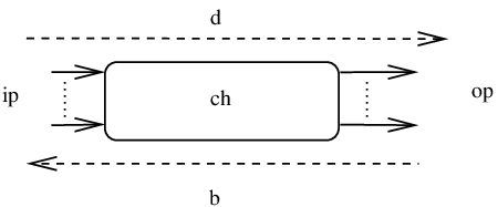
The corresponding module is depicted in Fig. 2.

Proof.

According to the conservation law (3), the number of packets in transit $P_{E}(t)$ in the edge $E$ at time $t\in\mathbb{T}^{u}$ obeys

P_{E}(t)=\int_{t_{0}(t)}^{t}\phi(\beta(E),s)ds

(6)

where $t_{0}(t)=t-T$ since the propagation delay is constant. A packet sent at time $t-T$ will indeed be, at time $t$ , still in the edge and about to leave. The result follows then from Proposition 3. ∎

We are now in a position to introduce transmission channel operators defining part of the network topology.

Definition 5.

The flow vectors $\phi(u^{-},t)=\col_{i}[\phi(u_{i}^{-},t)]$ , $\phi(b^{-},t)=\col_{i}[\phi(b_{i}^{-},t)]$ , $\phi(u^{+},t)=\col_{i}[\phi(u_{i}^{+},t)]$ and $\phi(b^{+},t)=\col_{i}[\phi(b_{i}^{+},t)]$ are related by transmission channel operators $\mathcal{R}_{\bullet}$ , $\bullet\in\{ub,bu,bb\}$ as

\begin{bmatrix}\phi(u^{-},t)\\ \phi(b^{-},t)\end{bmatrix}=\mathcal{R}\begin{bmatrix}\phi(u^{+},t)\\ \phi(b^{+},t)\end{bmatrix}+\mathcal{D}\delta(t)

(7)

where

\begin{array}[]{lclclcl}\mathcal{R}&=&\begin{bmatrix}0&\mathcal{R}_{ub}\\ \mathcal{R}_{bu}&\mathcal{R}_{bb}\end{bmatrix}&\mathrm{and}&\mathcal{D}&=&\begin{bmatrix}0\\ \mathcal{D}_{b}\end{bmatrix}.\end{array}

The matrices $\mathcal{R}_{\bullet}$ , $\bullet\in\{ub,bu,bb\}$ correspond to routing matrices between output and input nodes. For instance, $\mathcal{R}_{ub}$ maps flows at user output nodes to flows at buffer input nodes. These matrices essentially consist of constant delay operators with delays corresponding to transmission channels. The full-rank input matrix $\mathcal{D}_{b}$ drives the vector of cross-traffic flows $\delta(t)$ to buffer input nodes.

VI FIFO Buffer Model

This section is devoted to the very important buffer element which temporarily stores incoming information before processing it. First, the standard fluid model for queues is recalled [11, 3, 2] and a complete delay-map is characterized. In order assign each input flow to its corresponding output flow and solve the output flow separation problem [13, 14, 15, 16, 17, 18], the conservation law is then applied on the standard queue model, in a similar way as for transmission channels. The output separation problem allows us to focus on the accurate description of queues, which captures both the FIFO behavior and the form of output flows. Some extra discussions and interpretations of the results are also provided. Finally, a comparison to an existing model for output flows is carried out and concludes in favor of the proposed one.

VI-A Queue model

Routers have queues to store incoming packets temporarily. The following integrator model [11] can be proved to be a limit model of a M/M/1 queue when the packet size and thus the processing time tend to 0 [2, 19].

Definition 6.

The queue dynamics of buffer $b_{i}$ is governed by the model

\dot{q}_{i}(t)=\sum_{j=1}^{\sigma(b_{i})}\phi_{j}(b_{i}^{-},t)-r_{i}(t)

(8)

where the aggregate output rate is defined as

r_{i}(t)=\left\{\begin{array}[]{lcl}c_{i}&&\mathrm{if}\ \mathcal{C}_{i}(t)\\ \sum_{j}\phi_{j}(b_{i}^{-},t)&&\mathrm{otherwise}.\end{array}\right.

(9)

Above, $q_{i}$ , $c_{i}$ and $\phi_{j}(b_{i}^{-},t)$ represent the queue size, the maximal output capacity and the flow of type $j$ at the input respectively. The condition $\mathcal{C}_{i}(t)$ is given by

\mathcal{C}_{i}(t):=\left(\left[q_{i}(t)>0\right]\vee\left[\sum_{j}\phi_{j}(b_{i}^{-},t)>c_{i}\right]\right).

(10)

The corresponding queuing delay can be easily deduced using the relation $\tau_{i}(t)=q_{i}(t)/c_{i}$ . $\therefore$

The above model can also be refined to capture additional features such as finite maximal queue length, flow priorities, and multiple output capacities. These extensions are omitted here since they are straightforward. It is important to stress that this model is incomplete and useless in this form. First, the output flow is given in aggregate form. This prevents the modeling of the appropriate routing of each output flow. Second, it does not capture the queue FIFO behavior. Finally, the model does not assign a specific queueing time to each input flow. In the following subsection, the conservation law (3) is used in order to confer the FIFO property to the model and separate the aggregate output flow into distinct flows.

VI-B Forward and Backward Queuing Delays

The maps defined in this section are very useful for obtaining a closed formula for the buffer output flows in Section VI-C and for RTT in Section VII-C.

Let us consider first the buffer model (8) with queueing delay $\tau_{i}(t)$ . Assume that the time instants at which packets enter the queue are chosen as reference times. We may then be interested in predicting the packet output time. This leads to the following definition:

Definition 7 (Forward delay operator).

The forward delay operator $f_{i}:\mathbb{T}^{u}\to\mathbb{T}^{u}$ corresponding to buffer $b_{i}$ mapping, at a flow level, any input-time $t$ to the output-time $f_{i}(t)$ is defined as

f_{i}(t):=t+\tau_{i}(t)

(11)

where $\tau_{i}(t)$ is the queuing delay of buffer $b_{i}$ .

It is easy to see that output-time can be readily computed from the knowledge of input-time and queuing delay value. If however, we would like to set the reference time to be the output time, we may ask the question whether it is possible or not to retrieve the input-time from it. This is equivalent to asking the question of invertibility of the map $f_{i}$ .

Result 8 ([17]).

The map $f_{i}$ is invertible if and only if the input flow of the corresponding buffer is positive almost everywhere. $\blacktriangle$

Hence, provided that there is a nonzero input flow to the buffer, the input-time corresponding to a given output-time is well-defined and can be obtained using the backward delay operator:

Definition 9.

The backward delay operator $g_{i}:\mathbb{T}^{u}\to\mathbb{T}^{u}$ corresponding to buffer $b_{i}$ mapping, at a flow level, any output-time $t$ to the input-time $g_{i}(t)$ is defined as $g_{i}:=f_{i}^{-1}$ under the assumption of Result 8.

We also have the following useful results:

Result 10 ([17]).

The functions $f_{i}$ and $g_{i}:=f_{i}^{-1}$ obey:


$\displaystyle g_{i}^{\prime}(t)$	$\displaystyle=$	$\displaystyle\left\{\begin{array}[]{ll}\displaystyle{c_{i}\left(\sum_{k=1}^{\eta(b_{i})}\phi_{k}(b_{i}^{-},g_{i}(t))\right)^{-1}}&\mathrm{if\ }\mathcal{C}_{i}(g_{i}(t))\\ 1&\mathrm{otherwise}\end{array}\right.$
$\displaystyle f_{i}^{\prime}(t)$	$\displaystyle=$	$\displaystyle\left\{\begin{array}[]{lcl}\displaystyle{c_{i}^{-1}\sum_{k=1}^{\eta(b_{i})}\phi_{k}(b_{i}^{-},t)}&&\mathrm{if\ }\mathcal{C}_{i}(g_{i}(t))\\ 1&&\mathrm{otherwise}\end{array}\right.$
$\displaystyle{[\tau_{i}(g_{i}(t))]}^{\prime}$	$\displaystyle=$	$\displaystyle\left\{\begin{array}[]{lcl}1-\dfrac{c_{i}}{\sum_{k=1}^{\eta(b_{i})}\phi_{k}(b_{i}^{-},g_{i}(t))}&\mathrm{if\ }\mathcal{C}_{i}(g_{i}(t))\\ 1&\mathrm{otherwise}\end{array}\right.$

where $f^{\prime}(t)$ stands for the the upper right Dini derivative of $f(t)$ , i.e. ${f^{\prime}(t)=\limsup_{h\downarrow 0}h^{-1}\left(f(t+h)-f(t)\right).}$ $\blacktriangle$

The following technical result allows to simplify the conditions involved in hybrid models:

Result 11.

The equivalence $\mathcal{C}(g_{i}(t))\Leftrightarrow\mathcal{C}(t)$ holds.

Proof.

Proof of $\Rightarrow$ : If the buffer is congested at time $g_{i}(t)$ then the buffer will also be congested at time $t$ since the data entered at time $g_{i}(t)$ leave at time $t$ .
Proof of $\Leftarrow$ : Conversely, if there is any data to leave at time $t$ , they must have entered in the queue in the past, i.e. at time $g_{i}(t)$ . Equivalence is proved. ∎

VI-C FIFO Buffer Output Flow Separation

In this section, we use the results given above and the conservation law in order to improve the buffer modeling by adding the FIFO characteristics and splitting the aggregate output flows into a sum of distinct ones. Without further consideration on the queue type, there exists an infinite number of ways to separate the aggregate output flow directly from the queuing model of Definition 6. When a FIFO queue (i.e. order preserving) is considered, it turns out that the output flow separation problem is easily solvable. The FIFO characterization and output flow separation problems have been fully solved in [17]. In this section, we will simply recall and explain these results, and connect them to the conservation law (3).

Result 12 ([17]).

Let us consider the queueing model (8) which we assume to represent a FIFO queue. The output flow corresponding to the input flow $\phi_{\ell}(b_{i}^{-},t)$ , $\ell\leq\eta(b_{i}^{-})$ is given by

\begin{array}[]{lcl}\phi_{\ell}(b_{i}^{+},t)&=&g_{i}^{\prime}(t)\phi_{\ell}(b_{i}^{-},g_{i}(t))\\ &=&\left\{\begin{array}[]{lcl}\dfrac{c_{i}\phi_{\ell}(b_{i}^{-},g_{i}(t))}{\sum_{j}^{\eta(b_{i})}\phi_{j}(b_{i}^{-},g_{i}(t))}&&\mathrm{if\ }\mathcal{C}_{i}(t)\\ \phi_{\ell}(b_{i}^{-},t)&&\mathrm{otherwise}\end{array}\right.\end{array}

(13)

Proof.

A proof is available in [17]. A more direct one based on Proposition 3 is given here. Noting that for buffer $b_{i}$ , we have $t_{0}(t)=g_{i}(t)$ , then using Proposition (3) and the formulas of Result 10, we get equation (13) with the difference that the condition is $\mathcal{C}(g_{i}(t))$ . However, from Result 11, the condition $\mathcal{C}(g_{i}(t))$ is equivalent to $\mathcal{C}(t)$ and the result follows. ∎

The same model has been also proposed in [13, 16] but claimed without any proof. We have shown above that this model is an immediate consequence of the information conservation law and gives, for the first time, a theoretical proof for it. This considerably strengthens the trust we may have in this model. A comparison with packet-level simulations in the next subsection tends to show its exactness.

This model also deserves interpretation: formula (13) says that output flows consist of scaling and shifting of the input flows. The delay accounts for high flow viscosity and captures the queue FIFO behavior, at a flow level, while the nonlinear ratio expresses the flow coupling at the core of the flow and clock-coupling phenomena, see section III, since each output flow depends on the corresponding input flow and all the other ones as well. A change in a single flow will affect all the output flows. This model also tells that the output flow corresponding to the input flow $\phi_{\ell}(b^{-},t)$ is expressed as a (delayed) ratio of the input flow $\phi_{\ell}(b^{-},t)$ to the total input flow that entered the buffer at the same time. Hence, the output flows are proportional to relative flows modeling the ’chance’ of having a packet of certain type served at time $t$ . This ’chance’ is then scaled-up by the maximal output capacity to utilize the available capacity.

Operators representing buffers can now be introduced:

Definition 13.

The buffer operator $\mathcal{B}_{i}$ with $\eta(b_{i})$ input flows is defined as

\begin{array}[]{lcrclc}\mathcal{B}_{i}&:&\phi(b_{i}^{-},t)&\to&\phi(b_{i}^{+},t)\end{array}

(14)

where the output flows and the buffer state are governed by (8) and (13). Using these operators, we can build a matrix of operators $\mathcal{B}$ connecting the $\phi(b^{-},t)$ ’s to the $\phi(b^{+},t)$ ’s as

\phi(b^{+},t)=\mathcal{B}\phi(b^{-},t)

(15)

where $\mathcal{B}=\diag_{i}\left\{\mathcal{B}_{i}\right\}$ .

VI-D Comparison with Another Model

Two main models for buffer output flows have been reported in the literature on fluid-flow models: the flow-based model [13, 16, 17] described in this paper and the pseudo-queue-based one [14, 15, 18] given by

\phi_{\ell}(b_{i}^{+},t)=\left\{\begin{array}[]{lcl}\dfrac{q_{i}^{\ell}(t)c_{i}}{\sum_{k}q_{i}^{k}(t)}&&\mathrm{if}\ q_{i}(t)\neq 0\\ 0&&\mathrm{otherwise}\end{array}\right.

(16)

where $q_{i}^{\ell}(t)$ is the number of packets of type $\ell$ in queue $i$ and $c_{i}$ is the maximal output capacity of queue $i$ .

Until now, these models have not been confronted to each others. In the following, they will be theoretically and experimentally compared, and it will be shown that the flow-based model is the only model that faithfully characterizes the actual output flows, validating then the proposed conservation-law-based paradigm.

VI-D1 Theoretical argumentation

First, the above model assumes that the ’chance’ of having a packet of type $\ell$ at the output at time $t$ is $q_{i}^{\ell}(t)/\sum_{i}q_{i}^{\ell}(t)$ . Model (16) then makes no difference in picking a packet in the middle, at the end or at the beginning of the queue since only the number of packets matters. It is thus unable to capture the FIFO characteristic of the queue since swapping packets in the queue does not modify the output flow. In contrast, the proposed model does capture this characteristic through the delay dynamical model and the delayed nonlinear input-output relationship involving flows directly: relative variations of the input flows are passed to the output flows after some queueing delay. Note however that both models coincide at equilibrium.

Second, since output flows in model (16) are computed from the integration of input flows, it turns out that the map from input flows to output flows is a nonlinear low-pass filter with ’bandwidth’ equal to $1/q(t)$ when $q(t)>0$ . High frequencies in the input flows are hence filtered out, making the existing model inaccurate for high frequency flows (fast transient), especially when the queue size is large. Note that the actual buffer behavior does not have any filtering effect, it just behaves as an ordered tank. On the other hand, the proposed model does not filter out any frequency band due to its feedthrough structure. It however has a distortion effect on the input flows due to the nonlinear structure and the dynamically changing delay, i.e. change of frequency and amplitude. As a result, the queue-based model does not satisfy any conservation law since low-pass filters dissipate energy all over the frequency band, resulting in information loss at the model level. This is in total contradiction with the actual queue behavior that just stores information and does not dissipate anything. Note however that the flow-based model intrinsically satisfies the conservation since the model is derived from it.

Last, the proposed model incorporates naturally the queuing delay in the expression, while for model (16) it is unclear which delay to consider, since the order of arrival of data is not tracked.

VI-D2 Case Analysis

To compare the models, let us consider two input flows given by

\begin{array}[]{lcl}\phi_{1}(t)&=&(1+\beta)c\left(1+\Sq(\omega t)\right)/2,\\ \phi_{2}(t)&=&(1+\beta)c\left(1-\Sq(\omega t)\right)/2\end{array}

(17)

where $c>0$ and $\omega>0$ are the buffer output capacity and the oscillation of flows. The term $\beta>0$ is a tunable parameter related to the amplitude of the inputs flows and the function $\Sq(\omega t):=\sign(\sin(\omega t))$ is a square function of period $T:=2\pi/\omega$ . Since the flows are in phase opposition, they lead to an alternation of packet types in the queue while packet populations remain roughly close to each other at any time. Therefore, the output flows should reflect the actual content of the queues and the model should be able to keep track of the order of arrival of packets in the queue.

The queue-based model (16) predicts the queues

q_{i}(t)=\theta(t)q_{i}(0)+\int_{0}^{t}\theta(t-s)\phi_{i}(s)ds,\ i=1,2

(18)

with $\theta(t)=\left(\dfrac{q(0)}{q(0)+\beta ct}\right)^{1/\beta}$ from which it is quite difficult to foresee the shape of the output flows. We can however note that the filtering effect of the convolution operator with kernel $\theta$ will deform the input flows, making then the output flows not square anymore.

When the proposed flow-based model is considered, it is enough to compute the forward and backward delays, and apply the formula for output flows:

\begin{array}[]{lcl}\tau(t)&=&\beta t+\tau(0),\\ f(t)&=&(1+\beta)t+\tau(0),\\ g(t)&=&\dfrac{1}{1+\beta}(t-\tau(0)),\\ \phi_{1}(b^{+},t)&=&c(1+\Sq(\omega g(t)))/2,\\ &=&\dfrac{c}{2}\left[1+\Sq\left(\dfrac{\omega}{1+\beta}(t-\tau(0))\right)\right],\\ \phi_{2}(b^{+},t)&=&\dfrac{c}{2}\left[1-\Sq\left(\dfrac{\omega}{1+\beta}(t-\tau(0))\right)\right].\end{array}

(19)

In this case, the predicted output flows have the same shape as the input flows but with a different frequency and amplitude. The proposed output flow model then exactly captures the content of the queue, that is the alternation of blocks of size $N(T)$ of type 1 and type 2. It is also immediate to see that the number of packets $N(T)=N_{i}(T),\ i=1,2$ received by the buffer over one period $T$ is given by

N(T):=\int_{0}^{T}\phi_{1}(b^{+},s)ds=\dfrac{\pi(\beta+1)c}{\omega}.

(20)

By virtue of the information conservation law, the same number of packets is retrieved at the output over the period $(\beta+1)T$ , enlarged due to the limiting output capacity $c$ . It is quite convincing that the flow-based model yields a much more coherent picture for this example.

VI-D3 Simulation

For simulation, we choose $\omega=2\pi$ (i.e. $T=1$ s), $\beta=1$ , $c=100$ Mb/s and $\tau(0)=0$ . The output flows obtained from the different models are depicted in Fig. 5, where we observe the behaviors predicted by the above calculations. Notably, the output flows predicted by model (16) tend to slow-down (low pass-filtering effect), decrease along time and seem to both tend to $c/2$ , which is basically unrepresentative of the actual content and output of the queue. We can also notice the decrease of the bandwidth for the queue-based model as long as the queue grows in size.

For comparison with NS-2, which deals with packets rather than flows, we integrate (up to an additional constant) the output flows predicted by each model to obtain a number of packets so that the comparison with NS-2 makes sense. The results are depicted in Fig. 5 where we can see that the proposed model yields exactly the same results as NS-2 while the queue-based model is unable to track the stair-like curve returned by NS-2. It is also important to stress that the considered scenario is quite convenient for the queue-based model since the input flows contain mostly constant parts (low frequency parts). A very fluctuating input flow would be very penalizing and would make the low-pass filtering effect of the queue-based model even more apparent.

VII Complete user model - Window control

The derivation of the user model is, partially, still an open question and a complete solution, based on the conservation law (3), is proposed in this section. We assume that the implemented congestion control protocol admits a fluid-flow approximation, for instance interpolating the discrete-time trajectories of the real protocol [11, 20]. The conservation law is then applied over the circuit used by a user to obtain the so-called ACK-clocking model [21, 22] relating flight-size, user sending rate and RTT together. Several expressions for RTT are provided according to the considered reference time, similarly as for buffers. These results are finally merged together in order to clarify the connection between the flight-size and the user sending rate. The last step concerns the derivation of formulas relating the above variables to user congestion window size.

VII-A Protocol model

Here we assume that the congestion control algorithm can be represented as a continuous-time (hybrid) dynamical system. That is we have the following fact:

Fact 14.

There exist bounded functionals $\mathcal{P}_{i}$ , $\mathcal{W}_{i}$ and $\mathcal{U}_{i}$ such that the trajectories $(z_{i}(t),w_{i}(t))$ of the following continuous-time model defined over $\mathbb{T}^{u}$

\begin{array}[]{lcl}\dot{z}_{i}(t)&=&\mathcal{P}_{i}(z_{i}(t),\mu_{i}(t))\\ w_{i}(t)&=&\mathcal{W}_{i}(z_{i}(t),\mu_{i}(t))\\ \phi_{i}(u_{i}^{+},t)&=&\mathcal{U}_{i}(w_{i}(t),\phi_{i}(u_{i}^{-},t))\end{array}

(21)

match the trajectories of the asynchronous protocol (defined on $\mathbb{T}_{i}$ ) at points in $\mathbb{T}^{u}\cap\mathbb{T}_{i}$ . Above, $z_{i}$ , $\mu_{i}$ , $\phi_{i}(u_{i}^{-},\cdot)$ and $\phi_{i}(u_{i}^{+},\cdot)$ are the state of the protocol, the congestion measure, the acknowledgment flow rate and the user sending flow respectively. The window size, $w_{i}$ , is considered as the number of outstanding packets to track and supposed to be (weakly) differentiable.

A procedure to solve the above interpolation problem has been first proposed in [11] for TCP and has been adapted to FAST-TCP in [20, Appendix C.].

VII-B The ACK-Clocking model

The ACK-clocking model [21, 22] is a very important consequence of the conservation-law. It characterizes the flight-size⁵⁵ 5 The number of outstanding packets. $\digamma_{i}(C_{i},t):=P_{C_{i}}(t)$ of the user $u_{i}$ at any time $t\in\mathbb{T}^{u}$ over a circuit $C_{i}=\langle u_{i}^{+},u_{i}^{-}\rangle$ . The importance of the ACK-clocking model lies in the semantic; it adds to the model by relating RTT, flow and flight-size together⁶⁶ 6 Note however that in [22] the window size is considered instead of the flight-size, which is rather different. To make the distinction, the window-based ACK clocking model is denoted by W-ACK while the fligh-size-based one by FS-ACK. Equivalence holds when some conditions, such as ’flight-size $\geq$ window size’, are met. We will come back on this in Section VII-E.. With this result, it is possible to incorporate a number of important user properties and mechanisms into the corresponding model.

Result 15 (FS-ACK-Clocking).

The (FS)ACK clocking model is given by

\begin{array}[]{lcl}\digamma_{i}(C_{i},t+\RTT_{i}\{t\})&=&\displaystyle{\int_{C_{i}}\phi(\theta,t+\RTT_{i}\{t\})d\theta}\\ &=&\int_{t}^{t+\RTT_{i}\{t\}}\phi_{i}(u_{i}^{+},s)ds\end{array}

(22)

where $\RTT_{i}\{t\}$ is the RTT of a packet sent at time $t$ by user $u_{i}$ over the circuit $C_{i}$ . $\blacktriangle$

Proof.

Since flight-size is a number of packets in a circuit, it can be cast as a spatial integration over the corresponding circuit. Thus, according to the conservation-law, it is possible to convert the spatial integration into a temporal one provided that we can determine the integration bounds. To obtain them, we use the notion of RTT and suppose that a data sent by user $u_{i}$ in the circuit $C_{i}$ at time $t$ has a round-trip-time given by $\RTT_{i}\{t\}$ . This means that the packets sent between $t$ and $t+\RTT_{i}\{t\}$ are unacknowledged at $t+\RTT_{i}\{t\}$ and thus still in the circuit. Hence, the corresponding temporal integral has bounds $t$ and $t+\RTT_{i}\{t\}$ . ∎

VII-C Round-Trip-Time Models

The RTT consists of sum of a constant and a time-varying part, namely the propagation delays and the queuing delays, which have been characterized in Sections V and VI, respectively. By combining these results together, it is immediate to obtain a RTT based forward model on a forward circuit operator, which considers the packet input time as a reference.

To properly define it, let us consider a circuit $C$ with $N$ queues, indexed from 1 to $N$ . The indices $0$ and $N+1$ are used to denote the input and output nodes of the circuit respectively. Given a packet input time $t$ , the corresponding packet output time $t_{C}$ and RTT obey the following formulas based on the forward circuit operator $\mathscr{F}_{C}$ .

Definition 16.

The forward circuit operator $\mathscr{F}_{C}:\mathbb{T}^{u}\to\mathbb{T}^{u}$ of circuit $C$ assigned to any packet at input time $t$ , an output-time $t_{C}(t)$ is given by

\begin{array}[]{lcl}t_{C}(t)&=&\mathscr{F}_{C}(t),\\ \mathscr{F}_{C}&=&\nabla^{-1}_{N,N+1}\circ f_{N}\circ\nabla^{-1}_{N-1,N}\circ f_{N-1}\circ\ldots\\ &&\circ\nabla^{-1}_{2,3}\circ f_{2}\circ\nabla^{-1}_{1,2}\circ f_{1}\circ\nabla^{-1}_{0,1}\end{array}

(23)

where $\nabla_{i,j}$ is the constant delay operator with delay corresponding to the propagation delay between $i$ and $j$ and $\circ$ the composition operator. The corresponding RTT expression is then given by

\mathrm{RTT}\{t\}=t_{C}(t)-t=(\mathscr{F}_{C}-\mathrm{Id})(t)

(24)

where $\mathrm{Id}$ is the identity operator.

Formula (23) actually represents the alternation between constant delay operators corresponding to transmission channels delay (the $\nabla_{i}$ ’s) and the queuing delays corresponding to queues (the $f_{i}$ ’s). Example 18 illustrates this formula on the topology depicted in Fig. 1. The same formulas, albeit expressed in different ways, have been also obtained in [9, Section 3.3.5] and [22, equations (7d-7f)].

Although immediate to obtain, these expressions suffer from several drawbacks. First, operator $\mathscr{F}_{C}$ is clearly noncausal since it requires the knowledge of future information. Second, as pointed out in Section VI-B, the most convenient reference-time to use is the output time. In the user modeling problem, it coincides with the reception time of acknowledgments and the moment when the user receives the RTT information. Hence, it seems to be more convenient to consider a backward circuit operator based on the backward delay operator of Section VI-B. The existence of such an operator is immediately inferred from the existence of the backward delay operator.

Definition 17.

The backward circuit operator $\mathscr{B}_{C}:\mathbb{T}^{u}\mathbb{T}^{u}$ of circuit $C$ assigned to any packet at output time $t_{C}$ , an input-time $t(t_{c})$ is given by

\begin{array}[]{cll}\mathscr{B}_{C}&:=&\mathscr{F}_{C}^{-1},\\ t(t_{C})&=&\mathscr{B}_{C}(t_{C}),\\ \mathscr{B}_{C}&=&\nabla_{0,1}\circ g_{1}\circ\nabla_{1,2}\circ g_{2}\circ\nabla_{2,3}\circ\ldots\\ &&\circ g_{N-1}\circ\nabla_{N-1,N}\circ g_{N}\circ\nabla_{N,N+1}.\end{array}

(25)

Moreover, the corresponding RTT expression is given by

\mathrm{RTT}\{t\}=t_{C}-t(t_{C})=(\mathrm{Id}-\mathscr{B}_{C})(t_{C}).

(26)

It is important to stress that the RTT formula given above looks noncausal since the RTT of a packet sent at time $t$ is defined in terms of time $t_{C}>t$ . This is however not a problem since the RTT information is only available, and then used, by the user at time $t_{C}$ , when the ACK packet is actually received. What is important is the causality of the operator $\mathscr{B}_{C}$ in order to ensure computability of the RTT at any time. This emphasizes once again the relevance of considering output times as references. The example below illustrates the above discussions:

Example 18.

In the single-user/single-buffer case, the above expressions reduce to

\begin{array}[]{lcl}t_{C}(t)&=&t+T_{f}+T_{b}+\underbrace{\tau(t+T_{f})}_{\mbox{Future information}}\\ t(t_{C})&=&\underbrace{g(t_{C}-T_{b})}_{\mbox{Past information}}-T_{f}\\ \RTT\{t\}&=&t_{C}-t\\ &=&t_{C}-g(t_{C}-T_{b})+T_{f}\\ &=&T_{b}+T_{f}+\tau(g(t_{C}-T_{b}))\end{array}

(27)

where $T_{f}$ and $T_{b}$ are the forward and backward propagation delays corresponding to the constant delay operators $\nabla_{0,1}$ and $\nabla_{1,2}$ .

Using the backward expression of RTT and the relation $\mathscr{F}_{C_{i}}\circ\mathscr{B}_{C_{i}}=\mathscr{B}_{C_{i}}\circ\mathscr{F}_{C_{i}}=\mathrm{Id}$ , it easy to obtain the following result:

Result 19.

The flight size obeys

	$\displaystyle\digamma_{i}(C_{i},\mathscr{F}_{C_{i}}(t))$	$\displaystyle=$	$\displaystyle\int_{t}^{\mathscr{F}_{C_{i}}(t)}\phi(u_{i}^{+},s)ds$		(28)
	$\displaystyle\digamma_{i}(C_{i},t)$	$\displaystyle=$	$\displaystyle\int_{\mathscr{B}_{C_{i}}(t)}^{t}\phi(u_{i}^{+},s)ds.$		(29)

$\triangledown$

Proof.

This is an immediate consequence of the conservation-law (3) (through the ACK-clocking model) and the above RTT models. ∎

Note that in [22], a model is obtained directly from the W-ACK-clocking applied directly to a selected topology. However, the model is not modular itself since hand calculations are needed to make it implementable that results unfortunately in complexity very sensitive to the topology. Hence the objective of obtaining a metamodel is not attained. The reason is that the ACK-clocking model is used in implicit form while our proposed method incorporates solutions of it, yielding an explicit formulation achieving the characteristics of a metamodel, i.e. modularity and scalability.

VII-D ACK-Clocking Dynamics and User Flow Computation

Since the flight-size expression (29) is exactly of the form (3), then Proposition 3 can be immediately applied to derive an explicit expression for the output flow of a given circuit, that is the flow of received acknowledgments:

Result 20.

Let us consider a circuit $C_{i}=\langle u_{i}^{+},u_{i}^{-}\rangle$ . Then, the ACK-flow that user $u_{i}$ receives is given by

\phi(u_{i}^{-},t)=\mathscr{B}^{\prime}_{C_{i}}(t)\phi_{i}(u_{i}^{+},\mathscr{B}_{C_{i}}(t)).

(30)

$\triangledown$

Proof.

The key idea is to remark that $\digamma_{i}(C_{i},t)=N_{u_{i}^{+}}(t,\mathscr{B}_{C_{i}}(t))$ . Hence, using Proposition 3 and noting that the ACK-flow corresponds to the flow leaving the circuit $\phi(u_{i}^{-},t)$ , the result is obtained. Differentiability of $\mathscr{B}_{C_{i}}(t)$ is inferred from the differentiability of the backward delay operators. ∎

Note that differentiation of (29) yields

\phi_{i}(u_{i}^{+},t)=\digamma_{i}^{\prime}(C_{i},t)+\mathscr{B}^{\prime}_{C_{i}}(t)\phi_{i}(u_{i}^{+},\mathscr{B}_{C_{i}}(t))

(31)

meaning that to maintain a constant flight size, i.e. $\digamma_{i}^{\prime}(C_{i},t)=0$ , the user has to naturally send data at the same rate it receives ACK packets: this is exactly ACK-clocking but expressed at a flow level. By flow integration, we can easily recover the ’packet-level ACK-clocking’. A similar expression is reported in [18], but stated without proof and using the model in (16) to represent the buffer output flows. Once again the proposed methodology allows to provide strong mathematical foundations for some existing results.

VII-E User Flow, Flight-Size and Congestion Window Size

We need to clarify the relation between a user congestion window size $w_{i}(t)$ and its sending rate $\phi(u_{i}^{+},t)$ . First, recall that the congestion window size corresponds to the desired flight-size, while the flight-size is the current number of packets in transit. The window size is then a reference to track while the flight size is the controlled output. The control input is the user sending rate.

When the window size increases, the user can immediately send a burst of packets to equalize the flight- and window-sizes. In such a case, we can ideally assimilate them to be equal⁷⁷ 7 This is the main assumption in [22] justifying the use of the W-ACK-clocking model. (and so are their derivatives). The small delay corresponding to the protocol reaction time can be easily incorporated in the constant part of the RTT. The problem is, however, slightly more difficult when the congestion window size becomes smaller than the flight-size. In such a case, we can not withdraw packets from the network and the only thing we can do is to wait for the packets in the network to be acknowledged until, at some point, the flight size becomes equal to the window size. This basically means that the rate of decrease of the flight-size is equal to the rate of received acknowledgments (the rate at which data leave the network). Therefore, while positive slope of the flight-size is ideally unconstrained from above, the negative slope is lower bounded. In [9], a rate-limiter is a posteriori added to the model in order to constrain the negative slope of the flight size. This solution is however difficult to implement in the context of [9] due to the time-varying nature of the slope lower bound and the lack of any ACK-flow model. Note also that in most recent works [18, 22], this problem is automatically excluded by considering that the flight-size is always smaller than the window size, and that the window size does not decrease ‘too-much’. To the authors’ best knowledge no well-rounded solution has been provided yet for the problem of congestion window size decrease. We provide below an explicit and complete solution to this problem, regardless of the rate of the variation of congestion window size. This is achieved through an augmentation of the user model and the consideration of the flow of ACK packets.

According to the above discussion, the flight-size must obey

\digamma_{i}^{\prime}(C_{i},t)=\left\{\begin{array}[]{lcl}\dot{w}_{i}(t)&&\mathrm{if\ }\mathcal{T}_{i}(t)\\ -\phi(u_{i}^{-},t)&&\mathrm{otherwise}\end{array}\right.

(32)

where $\mathcal{T}_{i}(t)$ is a condition which is true when no lower limit on the rate of variation of the flight-size is imposed and false otherwise.

Result 21.

The flight-size $\digamma_{i}(C_{i},t)$ satisfies (32) if the user sending rate is defined as

\phi(u_{i}^{+},t)=\left\{\begin{array}[]{lcl}\dot{w}_{i}(t)+\phi(u_{i}^{-},t)&&\mathrm{if\ }\mathcal{T}_{i}(t)\\ 0&&\mathrm{otherwise}\end{array}\right.

(33)

where $\mathcal{T}_{i}(t)=\left([\pi_{i}(t)=0]\wedge[\dot{w}_{i}(t)+\phi(u_{i}^{-},t)\geq 0]\right)$ and

\dot{\pi}_{i}(t)=\left\{\begin{array}[]{lcl}0&&\mathrm{if\ }\mathcal{T}_{i}(t)\\ \dot{w}_{i}(t)+\phi(u_{i}^{-},t)&&\mathrm{otherwise}.\end{array}\right.

(34)

Moreover, this model is the simplest one. $\blacktriangle$

Proof.

The ACK-buffer $\pi_{i}$ , taking nonpositive values, measures the number of ACK packets to retain in order to balance the flight- and window-sizes. When the virtual buffer has negative state, i.e. $\pi_{i}(t)<0$ , the arriving ACK-packets have to be retained until the state reaches 0. Once zero is reached, the user can start sending again until the window size decreases too fast, i.e. $\dot{w}_{i}(t)<-\phi(u_{i}^{-},t)$ . Substitution of the user sending rate defined by (33) and (34) in (31) yields the flight-size behavior (32). To see that the model is minimal, it is enough to remark that both conditions in $\mathcal{T}_{i}(t)$ are necessary. ∎

In order to characterize the ACK-retaining mode, the ACK-buffer (34) has to be adjoined to the protocol model (21), resulting in an augmentation of the state of the user model. The protocol behavior depends on the measurements $\mu_{i}(\varkappa_{t})$ which are functions of the overall network state $\varkappa_{t}$ ; this state is discussed in more detail in Section VIII.

We are now in a position to define user operators from (33).

Definition 22.

The user operator $\mathcal{U}_{i}(w_{i}):\mathbb{R}_{+}\to\mathbb{R}_{+}$ mapping the ACK-flow $\phi(u_{i}^{-},t)$ to the sending flow $\phi(u_{i}^{+},t)$ is given by

\phi(u^{+},t)=\mathcal{U}(w)\phi(u^{-},t)

(35)

where $\mathcal{U}(w)=\diag_{i}\left\{\mathcal{U}_{i}(w_{i})\right\}$ and $\mathcal{U}_{i}$ is given in (21).

VIII General Network model

Modular and independent models for transmission channels, buffers and users have been developed in Sections V, VI and VII respectively. In this section we summarize the obtained results in a compact form involving dynamical systems and operators, and properties of the model are discussed. Notably, correspondence of the proposed model with existing ones is emphasized/recalled.

VIII-A General model

The general network model takes the form

\begin{array}[]{rcl}\dot{\varkappa}(t)&=&\mathcal{N}\left(\varkappa_{t},\phi(u^{-},t),\phi(b^{-},t)\right)\\ \digamma_{i}(C_{i},t)&=&\int_{\mathscr{B}_{C_{i}}(t)}^{t}\phi(u_{i}^{+},s)ds\end{array}

(36)

with

\Phi(t)=\begin{bmatrix}0&0&\mathcal{U}(w)&0\\ 0&0&0&\mathcal{B}\\ 0&\mathcal{R}_{ub}&0&0\\ \mathcal{R}_{bu}&\mathcal{R}_{bb}&0&0\end{bmatrix}\Phi(t)+\begin{bmatrix}0\\ 0\\ \hline\cr 0\\ \mathcal{D}_{b}\end{bmatrix}\delta(t)

(37)

where $\Phi(t)=\col(\phi(u^{+},t),\phi(b^{+},t),\phi(u^{-},t),\phi(b^{-},t))$ and $\varkappa=\col(\tau,z,\pi)$ are the flows and the state of the network, respectively. The hybrid models for user and queue dynamics are described by the nonlinear (discontinuous) functional $\mathcal{N}$ obtained from equations (8), (9), (21) and (34). The notation $\varkappa_{t}$ is here to emphasize that the evolution of the network state depends on past state values [23]. Note that adjoining the flight-size expression is needed to obtain a finite number of equilibrium points. Indeed, since the user flow is computed from the derivative of the flight-size, the equilibrium information is lost and can only be recovered from the original expression of the flight-size. At equilibrium we indeed have $\digamma_{i}^{*}=w_{i}^{*}=\RTT_{i}^{*}\phi_{i}^{*}$ where $\RTT_{i}^{*}$ and $\phi_{i}^{*}$ are equilibrium values for RTT and the sending flow of user $u_{i}$ , respectively.

This model thus takes the form of a descriptor nonlinear hybrid positive time-delay system with state-dependent and constant delays about which many theoretical questions are open: well-posedness, existence of solutions, uniqueness of solutions, stability of solutions, etc. Note also that in this paper, we have not discussed about delay-derivative constraints whose violation may lead to severe well-posedness problems [24], such as nonuniqueness of solutions, existence of small-solutions, stopping solutions, etc. Some simple topologies have been considered in [17] where it is shown that delay-derivative may exceed one under certain conditions. For the moment, it is unclear whether for arbitrary topologies and under certain reasonable conditions, the delays perceived by the users always have derivatives smaller than one. This property is very suitable for analysis since many theoretical tools can only been applied when this condition is verified, e.g. Lyapunov-Krasovskii functionals [25] or certain integral quadratic constraints [26].

VIII-B Model Approximations

The proposed framework includes explicit and seemingly exact expressions for every quantity of interest, but this was not historically the case. The sending rate model has always been a missing link in past formulations where ad-hoc models were considered. It has been recently shown in [9, 22] that these flow models are actually approximation of the W-ACK-clocking model, which is turn an approximation of the FS-ACK clocking model considered in this paper. We summarize these remarks below for completeness.

VIII-B1 Ratio flow model

By making the approximation $\digamma_{i}(t)\simeq w_{i}(t)$ in the FS-ACK-clocking model to get the W-ACK clocking model, we obtain

w_{i}(t)=\int_{\mathscr{B}_{C_{i}}(t)}^{t}\phi(u_{i}^{+},s)ds

(38)

and using the right-square rectangle rule we get the following expression for the sending rates

\phi(u_{i}^{+},t)\approx\dfrac{w_{i}(t)}{T_{i}+\tau(g^{i}(t))}

(39)

which is very similar to the ratio flow model for instance considered in [11, 7, 8].

VIII-B2 Joint flow model

The joint flow model reuses the W-ACK-clocking model and by making a first order Taylor expansion on the implicit expression

w_{i}(t)-\int_{t}^{\mathscr{F}_{C_{i}}(t)}\phi(u_{i}^{+},s)ds=0

(40)

we obtain

w_{i}(t)+(T_{i}+\tau(t+T_{i}^{f}))(\dot{w}_{i}(t)-\phi(u_{i}^{+},t))\approx 0

(41)

or equivalently

\phi(u_{i}^{+},t)\approx\dfrac{w_{i}(t)}{T_{i}+\tau(t+T_{i}^{f})}+\dot{w}_{i}(t)

(42)

which is exactly the joint flow model considered in [9, 19, 21, 20]. Neglecting the derivative term yields the usual ratio model [11, 7, 8].

VIII-B3 Static model

The static link model assumes that sending rates are proportional to the derivative of congestion window sizes, making the relation between these sizes and queuing delays static. This model can be obtained by further approximating the ratio model or using linearization and a (0,0) Padé approximation. In Section IX-B, a more general proof for the static-link model is provided and it suggests that the static model has a much wider domain of validity, as experimentally emphasized in [27].

IX The Single-Buffer/Multiple-User Topology with Delay-based Protocols

The purpose of this section is two-fold: exemplify the modeling technique on a simple topology and prove that when some conditions on the topology are met, the proposed model reduces to a model involving a static-link model [27]. The proposed model hence allows to clarify the status of the static-link model [27] by providing, for the first time, a mathematical proof for its domain of validity.

To this aim, a single-buffer/multiple-user topology connected by lossless transmission channels is considered. The forward and backward propagation delays of user $u_{i}$ are denoted by $T_{i}^{f}$ and $T_{i}^{b}$ respectively. We propose to use the following generic model of any delay-based congestion control protocol as the user model

\begin{array}[]{lcl}\dot{z}_{i}(t)&=&\mathcal{P}_{i}(z_{i}(t),\tau(g^{i}(t)))\\ w_{i}(t)&=&\mathcal{W}_{i}(z_{i}(t),\tau(g^{i}(t)))\end{array}

(43)

where $z_{i}$ , $w_{i}(t)$ , $T_{i}=T_{i}^{f}+T_{i}^{b}$ and $g^{i}(t)=g(t-T_{i}^{b})$ are the state of the protocol, the congestion window size, the propagation delay and the backward delay operator respectively. The functions $\mathcal{P}_{i}$ and $\mathcal{W}_{i}$ are defined as in (21).

IX-A Multiple-User/Single-Buffer Topology Model

The general model is given by (36) with (43) and

\small\begin{array}[]{rcl}\dot{\tau}(t)&=&\left\{\begin{array}[]{lcl}c^{-1}\sigma(t)+\delta(t)-1&&\mathrm{if\ }\mathcal{C}(t)\\ 0&&\mathrm{otherwise}\end{array}\right.\\ \dot{\pi}_{i}(t)&=&\left\{\begin{array}[]{lcl}0&&\mathrm{if\ }\mathcal{T}_{i}(t)\\ \dot{w}_{i}(t)+\phi(u_{i}^{-},t)&&\mathrm{otherwise}.\end{array}\right.\\ \digamma_{i}(t)&=&\int_{g^{i}(t)-T_{i}^{f}}^{t}\phi(u_{i}^{+},\theta)d\theta\\ \phi(u_{i}^{+},t)&=&\left\{\begin{array}[]{lcl}\dot{w}_{i}(t)+\phi(u_{i}^{-},t)&&\mathrm{if\ }\mathcal{T}_{i}(t)\\ 0&&\mathrm{otherwise}\end{array}\right.\\ \phi(u_{i}^{-},t)&=&\left\{\begin{array}[]{lcl}\frac{c\phi(u_{i}^{+},g^{i}(t)-T_{i}^{f})}{c\delta(g^{i}(t))+\sum_{j}\phi(u_{j}^{+},g^{i}(t)-T_{j}^{f})}&&\mathrm{if}\ \mathcal{C}(t)\\ \phi(u_{i}^{+},t-T_{i}^{b}-T_{i}^{f})&&\mathrm{otherwise}\end{array}\right.\\ \sigma(t)&=&\sum_{i=1}^{N}\phi(u_{i}^{+},t-T_{i}^{f})\end{array}

(44)

where $\delta(t)$ denotes the normalized cross-traffic ${\delta(t)\in[0,1)}$ . The topology of this model is completely described by (37) with the operators $\mathcal{B}$ , $\mathcal{U}=\diag_{i=1}^{N}\{\mathcal{U}_{i}\}$ , $\mathcal{R}_{ub}=\begin{bmatrix}\nabla_{T^{b}_{1}}&\ldots&\nabla_{T^{b}_{N}}\end{bmatrix}^{T}$ , $\mathcal{R}_{bb}=0$ and $\mathcal{R}_{bu}=\begin{bmatrix}\nabla_{T^{f}_{1}}&\ldots&\nabla_{T^{f}_{N}}\end{bmatrix}$ where $\nabla_{d}$ is the constant delay operator with delay $d>0$ .

IX-B Homogeneous Delays and No-Cross Traffic - The Static-Link Model

As stated in Section VIII-B3, the static-flow model can be obtained using various approximations, which suggest that the static-model is only valid locally. This however contradicts the results reported in [27] where it is emphasized that the static model may yield quite precise results over a wide domain. Note also that the static-link model has been invalidated in many scenarios, notably some involving very heterogeneous delays or cross-traffic, see e.g. [9] and examples of Section X. In the following, we show that the static model can be exact when some conditions on the network topology are met.

Assuming that the propagation delays are homogeneous, i.e. $T_{i}^{f}=T^{f}$ , $T_{i}^{b}=T^{b}$ , $i=1,\ldots,N$ , and that there is no cross-traffic, i.e. $\delta\equiv 0$ , the model in (44) reduces to

\begin{array}[]{lcl}\dot{\tau}(t)&=&\left\{\begin{array}[]{lcl}c^{-1}\sigma(t)-1&&\mathrm{if\ }\mathcal{C}(t)\\ 0&&\mathrm{otherwise}\end{array}\right.\\ \dot{\pi}_{i}(t)&=&\left\{\begin{array}[]{lcl}0&&\mathrm{if\ }\mathcal{T}_{i}(t)\\ \dot{w}_{i}(t)+\phi(u_{i}^{-},t)&&\mathrm{otherwise}.\end{array}\right.\\ \digamma_{i}(t)&=&\int_{g_{b}(t)-T^{f}}^{t}\phi(u_{i}^{+},\theta)d\theta\\ \phi(u_{i}^{+},t)&=&\left\{\begin{array}[]{lcl}\dot{w}_{i}(t)+\phi(u_{i}^{-},t)&&\mathrm{if\ }\mathcal{T}_{i}(t)\\ 0&&\mathrm{otherwise}\end{array}\right.\\ \phi(u_{i}^{-},t)&=&\left\{\begin{array}[]{lcl}\frac{c\phi(u_{i}^{+},g_{b}(t)-T^{f})}{\sum_{j}\phi(u_{j}^{+},g_{b}(t)-T^{f})}&&\mathrm{if}\ \mathcal{C}(t)\\ \phi(u_{i}^{+},t-T^{b}-T^{f})&&\mathrm{otherwise}\end{array}\right.\\ \sigma(t)&=&\sum_{i=1}^{N}\phi(u_{i}^{+},t-T^{f})\\ g_{b}(t)&=&g(t-T^{b}).\end{array}

(45)

Assuming further that the buffer is always congested (i.e. $\mathcal{C}(t)$ holds true for all $t$ ) and all users are active (i.e. the $\mathcal{T}_{i}(t)$ ’s are all true) we obtain

\dot{\tau}(t)=c^{-1}\sum_{i}\dot{w}_{i}(t-T^{f})

(46)

after the substitution of sending flows in queue dynamics. Integrating the above equation from $0$ to $t$ we obtain

\tau(t)=c^{-1}\sum_{i}w_{i}(t-T^{f})-T

(47)

where we assumed $\tau(0)=0$ and $w_{i}(0)=0$ , $i=1,\ldots,N$ . The additional constant term $-T$ can be determined such that the above equation satisfies the equilibrium equation $\sum_{i}w_{i}^{*}(T+\tau^{*})=c$ . Equation (47) is exactly the static model, showing then its exactness for the single-buffer/multiple-user topology with homogeneous propagation delays and no cross-traffic. This result might be generalizable to the case of chained buffers and multiple users. The exactness of the static model over more complex topologies is an open question. The case of single-buffer with constant cross-traffic may also be analyzable.

Thus, according to the model proposed in (44), the static-link model is exact in the single-link topology whenever

•

the buffers are permanently congested, i.e. $\mathcal{C}(t)$ holds true for all $t\geq 0$ ;
•

the propagation delays are homogeneous, i.e. $T_{i}^{f}=T^{f}$ , $T_{i}^{b}=T^{b}$ , $i=1,\ldots,N$ ;
•

the cross-traffic is absent, i.e. $\delta\equiv 0$ ;
•

the users are not in ACK-retaining mode, i.e. $\mathcal{T}_{i}(t)$ holds true for all $i=1,\ldots,N$ .

Compared to the justification of this model in [22], the proof developed above is much more insightful since no model approximation is made, only assumptions on the network topology. This shows that the static-link model has an application domain which is much wider than the ratio-link and the joint-link models, when the conditions on the topology are met. It is indeed valid in the nonlinear setting and it does not result from any approximation, just assumptions on the topology.

This also shows that the proposed metamodel is able to provide theoretical justifications of a simpler model. This supplies a way for deriving proofs for validity domain of models.

IX-C Homogeneous Delays and Cross-Traffic

When cross-traffic is added to the problem, the overall picture changes. The cross-traffic acts as a bandwidth limiter both in the networking and control terminology. Indeed, a nonzero $\delta(t)$ reduces the maximal output capacity $c$ , creating then sort of ‘varying-output-capacity’ $c(1-\delta(t))$ which reduces the bandwidth perceived by users.

Result 23.

In the congested mode, the queue model writes

\begin{array}[]{lcl}\dot{\tau}(t)&=&c^{-1}\sum_{i}\dot{w}_{i}(t-T^{f})+\delta(t)-\varphi(t)\\ \varphi(t)&=&\dfrac{c\delta(g_{bf}(t))}{c\delta(g_{bf}(t))+\sum_{j}\phi_{j}(u_{j}^{+},g_{bf}(t)-T^{f})}\end{array}

(48)

where $g_{bf}(t)=g(t-T^{b}-T^{f})$ and $\varphi(t)$ is the output flow at time $t$ corresponding to the cross-traffic. The term $\varphi(t)$ is responsible for the bandwidth reduction.

Proof.

Since the buffer is always congested and the users are not in ACK-retaining mode, we have

\phi_{i}(u_{i}^{+},t)=\dot{w}_{i}(t)+\phi_{i}(u_{i}^{-},t)

(49)

and

\phi_{i}(u_{i}^{-},t)=\dfrac{c\phi_{i}(u_{i}^{+},g_{b}(t)-T^{f})}{c\delta(g_{b}(t))+\sum_{j}\phi_{j}(u_{j}^{+},g_{b}(t)-T^{f})}.

(50)

Substituting the above expressions in the queue model and noting that $\sum_{j}\phi_{j}(u_{j}^{-},t-T^{f})+\varphi(t)=c$ yields the result. ∎

X Model Validation

We consider the scenarios given in [9, 22] to validate the proposed model. The results obtained via NS-2 have been slightly shifted in time so that the congestion window variation times match. Unlike [22], the results are not shifted in amplitude and this causes small discrepancies. If, however, the NS-2 results were shifted vertically so that they match initial equilibrium values, then the curves would match almost perfectly.

X-A Single-Buffer/Multiple-Users

Fig. 7: Topology of scenarios 1 & 2

In this section, we consider the interconnection of two users through a single resource, as depicted in Fig. 7. The bottleneck has capacity $c=100$ Mb/s and the packet size including headers is 1590 bytes. The following scenarios from [9, 22] are considered:

•

Scenario 1: the congestion window sizes are initially $w_{1}^{0}=50$ and $w_{2}^{0}=550$ packets, at 3s $w_{1}$ is increased to 150 packets. The propagation delays are $T_{1}=3.2$ ms and $T_{2}=117$ ms for users 1 and 2 respectively; see Fig. 9.
•

Scenario 2: the congestion window sizes are initially $w^{0}_{1}=210$ and $w_{2}^{0}=750$ packets, at 5s $w_{1}$ is increased to 300 packets. The propagation delays are $T_{1}=10$ ms and $T_{2}=90$ ms for users 1 and 2 respectively; see Fig. 9.

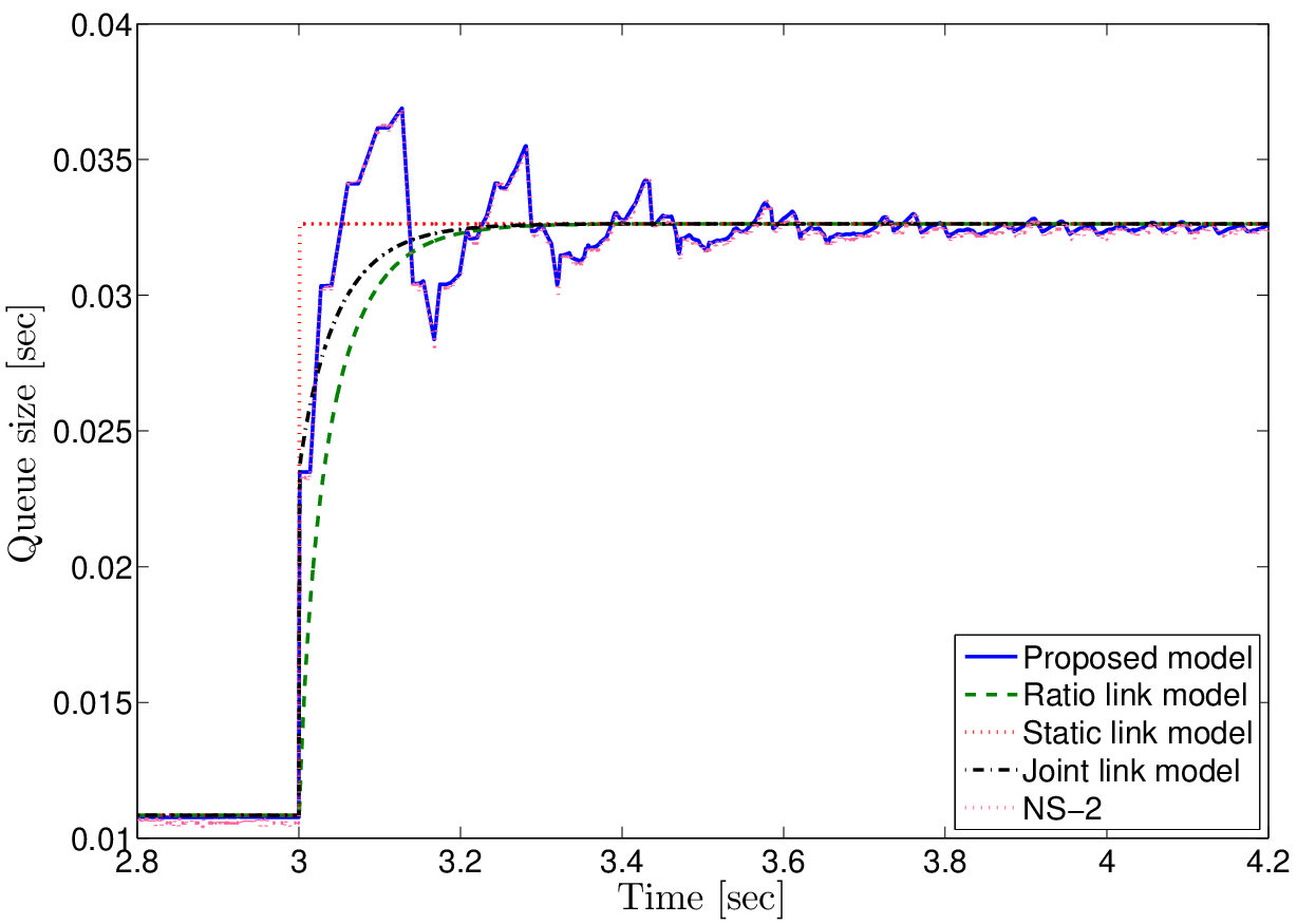
We can see that our results fit well with the ones obtained by packet level (NS-2) simulations. Yet, this is not the case for the ratio-link, static-link, and the joint-link models when the transient-state is considered. The obtained results by the proposed model are identical to the results given in [9, 22] and obtained using the W-ACK-clocking model. This is expected since the W-ACK clocking is an approximation of the FS-ACK-clocking model defended in this paper. Note also that the approximation condition related to the window size increase is satisfied here.

X-B Multiple-Buffers/Multiple-Users

Here, we consider the case of two buffers interconnected in series (see Fig. 10) with capacities $c_{1}=72$ Mb/s and $c_{2}=180$ Mb/s. The packet size including headers is $1448$ bytes. The link propagation delays are $20$ ms for link 1 and $40$ ms for link 2. The total round-trip propagation delays are $T_{1}=120$ ms, $T_{2}=80$ ms and $T_{3}=40$ ms for sources 1, 2 and 3 respectively. Initially, the congestion window sizes are $w_{1}^{0}=1600$ packets, $w_{2}^{0}=1200$ packets and $w_{3}^{0}=5$ packets. The following scenarios from [9, 22] are considered:

•

Scenario 3: No cross-traffic and the congestion window $w_{1}$ is increased by 200 packets at 10s; see Fig. 12.
•

Scenario 4: No cross-traffic and the congestion window $w_{2}$ is increased by 200 packets at 10s; see Fig. 12.

The proposed model is again able to capture the network behavior well and it retrieves the previous results reported in [9, 22]. This is again due to the equivalence between the ACK-clocking models in this case.

We introduce now a constant cross-traffic $x_{c1}=c_{1}/2$ on the first link. Initially⁸⁸ 8 This scenario is actually identical to the one in [22, Section III.B.3], the initial values for congestion window sizes given in [22] are incorrect., we set $w_{1}^{0}=1200$ , $w_{2}^{0}=1600$ , $w_{3}^{0}=5$ and we consider the following scenarios:

•

Scenario 5: The congestion window $w_{1}$ is increased by 200 packets at 10s; see Fig. 14.
•

Scenario 6: The congestion window $w_{2}$ is increased by 200 packets at 10s; see Fig. 14.

The obtained results are identical to the results obtained by the the NS-2 simulations. Notice the reaction time between the moment at which the congestion window size is increased and the moment at which the second queue sees the flow variation. This illustrates that the model captures well the communication path and the order of elements (spatial and temporal topology). These characteristics are not directly visible in the simulation results given in [22] since the curve steps seem to have been aligned on the same temporal cursor.

Despite of results equivalence, the proposed metamodel enjoys interesting properties such as modularity and scalability, that the model reported in [9, 22] lacks. This is an important improvement over previous models that were not able to cumulate accuracy, scalability, modularity and other interesting properties. This will be discussed in more detail in the next Section.

X-C Decreasing the Congestion Window Size

The models proposed in [18, 22] do not capture sudden decreases in the congestion window size that would cause the buffer to empty or become smaller than the actual flight-size, that is, smaller than the number of packets in flight. The proposed model does capture these phenomena since 1) the FS-ACK-clocking model derived from the conservation law involves the flight-size rather than the congestion window size, unlike in [22]; and 2) the user model implements an ACK-buffer to count the number of packets to remove from the network before starting to send again. Note that the derivation of the user model including the ACK-buffer has been made possible due to the availability of an explicit expression for the flow of acknowledgments (30). This makes it computable through an explicit solution for the queuing delay and the buffer output flows [17, 28]. In [9], the decreasing of congestion window size is handled by adding a rate limiter to constrain the (negative) slope of the queue size. This rate limiter is however rather difficult to characterize due to the time-varying nature of the lower-bound on the slope which depends on the received rate of acknowledgment and the network state, the former being unfortunately unavailable in the framework of the thesis [9].

Let us consider the single-user/single-buffer case where the total propagation delay is $T=150$ ms, the packet size including headers is $1040$ bytes and the initial value of the congestion window size is $w^{0}=500$ . A $t=5$ seconds, the congestion window size is halved. We consider the following scenarios

•

Scenario 7: $c=12.5$ Mb/s and no cross-traffic; see Fig. 16.
•

Scenario 8: $c=25$ Mb/s and half capacity used by cross-traffic; see Fig. 16.

We can see that we obtain exactly the same results as NS-2 simulations (and the rate-limiter model reported in [9]). As desired, the ACK-buffer measures (counts) the number of packets to remove before starting to send again.

XI Related Work

Despite of being unorthodox, it was to the authors’ point of view to discuss the related works after presenting the proposed metamodel. Many congestion models have been proposed in the literature with different formalisms: time-domains, protocols, network topologies and other hypotheses. It is thus quite difficult to compare them directly and give a thorough discussion. Yet, we have identified some important characteristics which are summarized in Tables I, II and III. Table I collects global characteristics of a network model such as the time-domain property to indicate whether the model is in discrete (DT) or continuous (CT) time, or the modularity property to indicate whether it is modular or not. With delay we indicate that the model considers it either as constant (Cst), time-varying (TV), state-dependent (SD), or asynchronous (Async) discrete-time system whose asynchrony (incorporating delays) depends on the state of the system. Spatial and temporal topologies denote whether the model share the same spatial and time topologies with the actual network, respectively. Generic indicates the ability of the model to describe the network for different protocols whereas rate model denotes from which formula the user sending rate is computed. The ratio flow model [11, 14, 7, 15, 8] is given by quotient of the congestion window size and the RTT. The static flow model [27] assumes that the flow is proportional to the derivative of the congestion window size and the joint flow model [9, 19, 21, 20] assumes that the flow is given by the sum of the ratio-flow model and the congestion window size derivative.

Tables II and III examine the important subparts of the model, namely the user and buffer models, respectively. It is also important to mention that none of them has the structure of a metamodel having the precision of the considered one. In Table II, homogeneous and heterogeneous delays denote how well a model captures the case of homogeneous or heterogeneous propagation delays, whereas cross and bursty traffic denote how well a model captures the presence of cross traffic and bursty traffic [29], respectively. Exact indicates that the transient-state behavior of a model matches well to the one observed in packet level simulations. Too fast and too slow mean that a model converges to steady-state faster or slower, respectively, compared to what is observed in packet level simulations. Faster states a relativity faster convergence, yet not as much as observed when it is too fast. In Table III, output flows indicates whether it is defined as aggregate, meaning all input flows are mixed, or split, where the buffer acts as a square MIMO system mapping a given input flow to a given output flow. FIFO characterization denotes whether the model captures the actual content of the queue and the FIFO behavior. With queuing delay model we indicate whether its effect on input flows are clearly defined. Frequency filtering effect denotes whether the model of buffer have a filtering effect on the input flows to the output flows.

Network Models	[30]	[7]	[11]	[31]	[27]	[9] (DAE)	[32]	[15]	[33]	[22]	This paper
Characteristics
Time-domain	DT	CT	CT	CT	CT	DT	CT	Hybrid	DT	CT	Hybrid
Delay	Cst	Cst	TV/SD¹¹footnotemark: 1	Cst	Cst	Async.	Cst	Cst	Async.	SD²²footnotemark: 2 .	SD
Modular	Almost³³footnotemark: 3	Yes	No	Yes	Yes	No	Yes	Almost⁴⁴footnotemark: 4	No	Almost⁵⁵footnotemark: 5	Yes
Spatial topology	Yes	No	Yes	No	Yes	Yes	Yes	No	Yes	Yes	Yes
Temporal topology	Yes	No	Yes	No	Yes	Yes	Yes	Yes	Yes	Yes	Yes
Generic	Yes	No	No	No	No	No	No	No	Yes	Yes	Yes
Rate model	No⁶⁶footnotemark: 6	Ratio	Ratio	Ratio	Static	(FS)ACK⁷⁷footnotemark: 7	Joint	Ratio	No⁶⁶footnotemark: 6	(W)ACK⁸⁸footnotemark: 8	(FS)ACK⁹⁹footnotemark: 9

TABLE I: Main characteristics of some existing models in the literature.

XI-1 Table I

¹In this model, while the delay is denoted as a function of time, it is implicitly defined from the state, without further investigation. An exact delay characterization as a function of the state has been obtained in [17]. ²The state-dependent delay is implicitly characterized by the ACK-clocking formula and the RTT expression. ³The modularity of the model could have been developed but was not. ⁴Modular but not able to represent any topology, essentially due to lack of any output flow model for buffers. ⁵This modeling technique can be applied to any type of topology, however hand calculations, which result in poor scalability, are necessary. ⁶The notion of flow is not defined in a discrete-time model. ⁷The discrete-time model is derived from a continuous-time model using the (FS)ACK-clocking model. ⁸The flow is implicitly defined as the solution of the (W)ACK-clocking model. ⁹The flow is computed by solving the (FS)ACK-clocking model explicitly.

	User sending flow models	Static	Ratio	Joint	(W)ACK	(FS)ACK+
	User sending flow models	Static	Ratio	Joint	(W)ACK	ACK-Buffer¹⁰¹⁰footnotemark: 10
Congestion window	Characteristics
Increase	Homogeneous delays	Exact/Too fast¹¹¹¹footnotemark: 11	Too slow¹⁴¹⁴footnotemark: 14	Faster¹²¹²footnotemark: 12	Exact	Exact
	Heterogeneous delays	Too fast	Too slow¹⁴¹⁴footnotemark: 14	Faster¹²¹²footnotemark: 12	Exact	Exact
	Cross-traffic	Too fast¹³¹³footnotemark: 13	Too slow¹⁴¹⁴footnotemark: 14	Faster¹²¹²footnotemark: 12	Exact	Exact
	Bursty-traffic	Exact/Too fast¹⁵¹⁵footnotemark: 15	Too slow¹⁴¹⁴footnotemark: 14	Faster¹⁶¹⁶footnotemark: 16	Exact	Exact
Decrease	Homogeneous delays	Too fast¹⁷¹⁷footnotemark: 17	Too slow¹⁴¹⁴footnotemark: 14	Too slow¹⁴¹⁴footnotemark: 14	Too fast¹⁷¹⁷footnotemark: 17	Exact
	Heterogeneous delays	Too fast¹⁷¹⁷footnotemark: 17	Too slow¹⁴¹⁴footnotemark: 14	Too slow¹⁴¹⁴footnotemark: 14	Too fast¹⁷¹⁷footnotemark: 17	Exact
	Cross-traffic	Too fast¹⁷¹⁷footnotemark: 17	Too slow¹⁴¹⁴footnotemark: 14	Too slow¹⁴¹⁴footnotemark: 14	Too fast¹⁷¹⁷footnotemark: 17	Exact

TABLE II: Comparison of different user flow models with respect to the accuracy of estimated queue sizes.

XI-2 Table II

¹⁰This model is the one introduced in [28] and also considered in the current paper. ¹¹In the single-buffer case the model is exact. It is unclear whether this is also true for the multiple buffer case. In most cases, the model is too fast. ¹²Accurate modeling of discontinuity/high slope of the queue when burst of data arrives at the queue input. ¹³The model is usually too fast. It might, however, be possible to refine it to account for constant cross-traffic [19]. ¹⁴Unable to characterize the high slope of the queue due to the low-pass filtering effect of the resulting queue model, see Section VI-D. ¹⁵Exact in the case of homogeneous delays and single-buffer topology since the relation is static and it has an infinite bandwidth; see Section IX-B. Too fast otherwise. ¹⁶Larger bandwidth than the ratio model but still limited since the bandwidth reduces as the queue size grows. ¹⁷These models may withdraw packets from the network by injecting negative flows.

Buffer descriptions	Aggregate model (8)-(9)	Pseudo-queue model [15, 18]	Flow model [13, 16, 17]
Characteristics
Output flows	Aggregate	Split	Split
FIFO characterization	Lost¹⁸¹⁸footnotemark: 18	No¹⁹¹⁹footnotemark: 19	Yes²⁰²⁰footnotemark: 20
Queuing delay model	Lost¹⁸¹⁸footnotemark: 18	No²¹²¹footnotemark: 21	Yes ²²²²footnotemark: 22
Frequency filtering effect	All-pass/undef.²³²³footnotemark: 23	All-pass/Low-pass²⁴²⁴footnotemark: 24	All-pass ²⁵²⁵footnotemark: 25

TABLE III: Comparisons between different buffer descriptions.

XI-3 Table III

¹⁸The information is lost since the output flows are aggregate. ¹⁹The output flows are insensitive to content swapping. ²⁰The output flows are sensitive to any swap of information in the queue. ²¹The exact queuing delay is actually difficult to assign to any output flow due to the structure of the model for the output flows involving queues. ²²Undefined due to the aggregate formalism. ²³All-pass when the sum of the input-flows does not exceed the maximal output capacity, otherwise the filtering effect is not really defined due to the aggregate formalism. ²⁴All-pass when the sum of the input-flows does not exceed the maximal output capacity, otherwise acts as a low-pass filter with bandwidth inversely proportional to the queue size. ²⁵This is due to the direct-feedthrough structure of the model. The delay and nonlinear formula for the output flows only have a compressing/expanding effect on time and amplitude.

XII Conclusion

This paper presents a modular fluid-flow network congestion control model to analyze communication networks with arbitrary topology. This modular metamodel is introduced by mathematically modeling network elements such as queues, users, and transmission channels, and network performance indicators such as sending/acknowledgement rates and delays. It is composed of building blocks that implement local mechanisms, some of which being ignored/unmodeled by some existing models in the literature. It is shown that the proposed model allows to recover existing models and brings a formal proof for their validity/invalidity as well as for their domain of validity. We present a novel classification of the previously proposed models in the literature and we show that the existing models are often not capable of capturing the transient behavior of the network precisely. Numerical results obtained from packet-level simulations demonstrate the accuracy of the proposed model. We plan to extend our work with modeling of data loss, such as packet drops, and the time-out mechanism at the user level.

XIII Acknowledgment

This work is dedicated to the memory of our colleague Prof. Ulf T. Jönsson, who unfortunately passed away before he could see it completed.

References

[1] V. Jacobson, “Congestion avoidance and control,” SIGCOMM Comput. Commun. Rev., vol. 18, no. 4, pp. 314–329, 1988.
[2] R. Srikant, The Mathematics of Internet Congestion Control. Boston, USA: Birkhäuser, 2004.
[3] S. Low, F. Paganini, and J. C. Doyle, “Internet congestion control,” IEEE Control Systems Magazine, pp. 28–43, February 2002.
[4] D. Mitra, “Stochastic theory of a fluid model of producers and consumers coupled by a buffer,” Advances in Applied Probability, vol. 20(3), pp. 646–676, 1988.
[5] R. Johari and D. Tan, “End-to-end congestion control for the internet: delay and stability,” Statistical Laboratory, University of Cambridge, Technical report, 2000.
[6] C. Hollot, V. Misra, D. Towsley, and W. B. Gong, “A control theoretic analysis of RED,” in 20th IEEE Conference on Computer Communications (INFOCOM), Tel-Aviv, Israel, 2001, pp. 1510–1519.
[7] G. Vinnicombe, “On the stability of networks operating TCP-like congestion control,” in 15th IFAC World Congress, Barcelona, Spain, 2002, pp. 217–222.
[8] F. Pagaganini, J. C. Doyle, and S. Low, “A control theoretical look at internet congestion control,” in Multidisciplinary Research in Control, ser. Lecture Notes in Control and Information Sciences, L. Giarré and B. Bamieh, Eds. Springer Berlin / Heidelberg, 2003, vol. 289, pp. 17–31.
[9] K. Jacobsson, “Dynamic modeling of internet congestion control,” Ph.D. dissertation, KTH School of Electrical Engineering, 2008. [Online]. Available: https://eeweb01.ee.kth.se/upload/publications/reports/2008/TRITA-EE_2008_020.pdf
[10] D. V. Lindley, “The theory of queues with a single server,” Mathematical Proceedings of the Cambridge Philosophical Society, vol. 48, pp. 277–289, 1952.
[11] V. Misra, W. Gong, and D. Towsley, “Fluid-based analysis of a network of AQM routers supporting TCP flows with an application to RED,” in ACM SIGCOMM’00, Stockholm, Sweden, 2000.
[12] G. Vinnicombe, “On the stability of end-to-end congestion control for the internet,” University of Cambridge, Technical report CUED/F-INFENG/TR 398, 2000.
[13] C. Ohta and F. Ishizaki, “Output processes of shaper and switch with self-similar traffic in ATM networks,” IEICE Transactions on Communications, vol. E81-B(10), pp. 1936–1940, 1998.
[14] J. Hespanha, S. Bohacek, K. Obraczka, and J. Lee, “Hybrid modeling of TCP congestion control,” in Hybrid Systems: Computation and Control, ser. Lecture Notes in Computer Science, M. Di Benedetto and A. Sangiovanni-Vincentelli, Eds. Springer Berlin / Heidelberg, 2001, vol. 2034, pp. 291–304.
[15] D. Färnqvist, K. Strandemar, K. H. Johansson, and J. P. Hespanha, “Hybrid modeling of communication networks using modelica,” in Proc. of the Radiovetenskap och Kommunikation (RVK), 2002.
[16] Y. Liu, F. L. Presti, V. Misra, D. F. Towsley, and Y. Gu, “Scalable fluid models and simulations for large-scale ip networks,” ACM Trans. Model. Comput. Simul., vol. 14(3), pp. 305–324, 2004.
[17] C. Briat, H. Hjalmarsson, K. H. Johansson, G. Karlsson, U. T. Jönsson, and H. Sandberg, “Nonlinear state-dependent delay modeling and stability analysis of internet congestion control,” in 49th IEEE Conference on Decision and Control, Atlanta, USA, 2010, pp. 1484–1491.
[18] Y. Zhang, Y. Xiang, S. Liu, and D. Loguinov, “Queuing dynamics and single-link stability of delay-based window congestion control,” Computer Networks, vol. 54, pp. 1543–1553, 2010.
[19] N. Möller, “Window-based congestion control,” Doctoral thesis, KTH, Stockholm, Sweden, 2008. [Online]. Available: https://eeweb01.ee.kth.se/upload/publications/reports/2008/TRITA-EE_2008_001.pdf
[20] K. Jacobsson, L. Andrew, A. Tang, S. Low, and H. Hjalmarsson, “An improved link model for window flow control and its application to FAST TCP,” IEEE Transactions on Automatic Control, vol. 54(3), pp. 551–564, 2009.
[21] K. Jacobsson, L. Andrew, A. Tang, K. H. Johansson, H. Hjalmarsson, and S. Low, “ACK-clock dynamics: Modeling the interaction between ACK-clock and network,” in 27th IEEE Conference on Computer Communications (INFOCOM), Phoenix, Arizona, USA, 2008, pp. 181–185.
[22] A. Tang, L. L. H. Andrew, K. Jacobsson, K. H. Johansson, H. Hjalmarsson, and S. H. Low, “Queue dynamics with window flow control,” IEEE/ACM Transactions on Networking, vol. 18(5), pp. 1422–1435, 2010.
[23] J. K.Hale and S. M. V. Lunel, Introduction to Functional Differential Equations. New York, USA: Springer-Verlag, 1991.
[24] W. Michiels and E. Verriest, “A look at fast varying and state dependent delays from a system theory point of view,” K.U. Leuven, Internal Report, 2011. [Online]. Available: http://www.cs.kuleuven.be/publicaties/rapporten/tw/TW586.abs.html
[25] K. Gu, V. Kharitonov, and J. Chen, Stability of Time-Delay Systems. Birkhäuser, 2003.
[26] C. Kao and A. Rantzer, “Stability analysis of systems with uncertain time-varying delays,” Automatica, vol. 43, pp. 959–970, 2007.
[27] J. Wang, D. X. Wei, and S. H. Low, “Modelling and stability of FAST TCP,” in 28th IEEE Conference on Computer Communications (INFOCOM), 2005, pp. 938–948.
[28] C. Briat, H. Hjalmarsson, K. H. Johansson, G. Karlsson, U. T. Jönsson, H. Sandberg, and E. A. Yavuz, “An axiomatic fluid-flow model for congestion control analysis,” in 50th IEEE Conference on Decision and Control, Orlando, Florida, USA, 2011, pp. 3122–3129.
[29] H. Jiang and C. Dovrolis, “Why is the internet traffic bursty in short time scales?” in Proceedings of the 2005 ACM SIGMETRICS International Conference on Measurement and Modeling of Computer Systems, ser. SIGMETRICS ’05, 2005, pp. 241–252.
[30] R. Johari and D. K. Tan, “End-to-end congestion control for the internet - delays and stability,” IEEE/ACM Transactions on Networking, vol. 19(6), pp. 818–832, 2001.
[31] F. Paganini, Z. Wang, J. C. Doyle, and S. Low, “Congestion control for high performance, stability, and fairness in general networks,” IEEE/ACM Transactions on Networking, vol. 13, no. 1, pp. 43–56, 2005.
[32] A. Tang, K. Jacobsson, L. L. H. Andrew, and S. H. Low, “An accurate link model and its application to stability analysis of FAST TCP,” in 26th IEEE Conference on Computer Communications (INFOCOM), Anchorage, Alaska, USA, 2007, pp. 161–169.
[33] R. Shorten, F. Wirth, and D. Leith, “A positive systems model of TCP-like congestion control: asymptotic results,” IEEE Transactions on Networking, vol. 14(3), pp. 616–629, 2006.