跳到论文正文
W Papers独立论文阅读器 arXiv:1303.3787 论文正文 计算阅读时间 · 0%
引用这篇论文根据当前论文元数据生成,正式投稿前建议核对。


License: CC BY-NC-SA 4.0
arXiv:1303.3787v5 [astro-ph.CO] 17 Dec 2024

Encyclopædia Inflationaris

https://github.com/cosmicinflation/aspicarXiv: 1303.3787
Jérôme Martin Affiliation: Institut d’Astrophysique de Paris, UMR 7095-CNRS, Université Pierre et Marie Curie, 98bis boulevard Arago, 75014 Paris (France) Email: jmartin@iap.fr    Christophe Ringeval Affiliation: Institut d’Astrophysique de Paris, UMR 7095-CNRS, Université Pierre et Marie Curie, 98bis boulevard Arago, 75014 Paris (France) Affiliation: Cosmology, Universe and Relativity at Louvain, Institute of Mathematics and Physics, Louvain University, 2 Chemin du Cyclotron, 1348 Louvain-la-Neuve (Belgium) Email: christophe.ringeval@uclouvain.be    Vincent Vennin Affiliation: Institut d’Astrophysique de Paris, UMR 7095-CNRS, Université Pierre et Marie Curie, 98bis boulevard Arago, 75014 Paris (France) Affiliation: Laboratoire de Physique de l’École Normale Supérieure, ENS, CNRS, Université PSL, Sorbonne Université, Université Paris Cité, 75005 Paris (France) Email: vincent.vennin@ens.fr
today
Abstract

The current flow of high-accuracy astrophysical data, among which are the Cosmic Microwave Background (CMB) measurements by the Planck satellite, offers an unprecedented opportunity to constrain the inflationary theory. This is however a challenging project given the size of the inflationary landscape which contains hundreds of different scenarios. Given that there is currently no observational evidence for primordial non-Gaussianities, isocurvature perturbations or any other non-minimal extension of the inflationary paradigm, a reasonable approach is to consider the simplest models first, namely the slow-roll single-field models with minimal kinetic terms. This still leaves us with a very populated landscape, the exploration of which requires new and efficient strategies. It has been customary to tackle this problem by means of approximate model-independent methods while a more ambitious alternative is to study the inflationary scenarios one by one. We have developed the publicly available runtime library ASPIC to implement this last approach. The ASPIC code provides all routines needed to quickly derive reheating-consistent observable predictions within this class of scenarios. ASPIC has been designed as an evolutive code which presently supports 118118 different models. In this paper, for each of the ASPIC models, we present and collect new results in a systematic manner, thereby constituting the first Encyclopædia Inflationaris.

Keywords
Cosmic Inflation, Slow-Roll, Reheating, Cosmic Microwave Background, Aspic
††subheader: Opiparous Edition

Dedicated to Jean Le Rond d’Alembert (1717–1783) and Denis Diderot (1713–1784).

Le but d’une encyclopédie est de rassembler les connaissances éparses sur la surface de la terre; d’en exposer le système général aux hommes avec qui nous vivons, et de les transmettre aux hommes qui viendront après nous; afin que les travaux des siècles passés n’aient pas été des travaux inutiles pour les siècles qui succéderont; que nos neveux, devenant plus instruits, deviennent en même temps plus vertueux et plus heureux, et que nous ne mourions pas sans avoir bien mérité du genre humain.

Preface to the new edition

The first edition of Encyclopædia Inflationaris [1] compiles the single-field slow-roll models of inflation that were proposed prior to 2013. It contains accurate reheating-consistent slow-roll calculations of the dynamics of the background universe in these models, as well as of cosmological scalar and tensor perturbations. Although it is often seen as a review, it goes beyond the mere gathering of known results, since a fair fraction of these models had been studied only under rough approximations, which do not match the need for high accuracy from current and forthcoming cosmological data. The ambition of the encyclopaedic project is instead to provide an (almost) exact treatment of these models, using only the slow-roll approximation, and incorporating the effects of reheating on the scale correspondence in a consistent way. All these results are incorporated in a public library, ASPIC [2], standing for “Accurate Slow-roll Predictions for Inflationary Cosmology”, which has been used in a number of subsequent works, as for instance in the Particle Data Group [3]. Bayesian model comparison using the Cosmic Microwave Background (CMB) data has been presented in Refs. [4, 5] while the constraints derived on the reheating epoch have been separately presented in Refs. [6, 7, 8].

Ten years later, inflation remains the most favored scenario of the early universe [9] but several developments call for the release of a new edition. First, at the theoretical level, new models have been proposed. Some of them boil down to one of the functional forms of the inflationary potentials already encoded in ASPIC, in which case they have been added in the relevant sections11 1 These models may nonetheless come with different values for the parameters describing the potential, i.e. different priors in the framework of a Bayesian analysis.. Some other models give rise to new inflationary potentials, and therefore constitute new sections of Encyclopædia Inflationaris, as well as new entries in the ASPIC library. There are 24 such new potential functions in the new edition (here ordered alphabetically): Axion Hilltop Inflation (AHI), Cubicly Corrected Starobinsky Inflation (CCSI), Double Exponential Inflation (DEI), Dual Inflation (DI), Fibre Inflation (FI), Generalized Double Well Inflation (GDWI), Hyperbolic Inflation (HBI), Hybrid Natural Inflation (HNI), Non-Renormalizable Corrected Loop Inflation (NCLI), N-Formalism Inflation (NFI), Non-Minimal Large Field Inflation (NMLFI), Pure Arctan Inflation (PAI), Radiatively Corrected Inflection Point Inflation (RCIPI), Radiatively Corrected Large Field Inflation (RCLFI), String Axion Inflation I (SAII), String Axion Inflation II (SAIII), Super-conformal Alpha Attractor A Inflation (SAAI), T-Model Inflation (TMI), Super-conformal Alpha Attractor B Inflation (SABI), Super-conformal Alpha Attractor T Inflation (SATI), Symmetry Breaking Kähler Inflation (SBKI), S-Dual Inflation (SDI), Smeared Higgs Inflation (SHI), Mukhanov Inflation (VFMI). The inclusion of these models allows the new edition to provide an up-to-date landscape of all single-field slow-roll inflationary models, bringing the number of models included in the ASPIC library to 118.

Second, at the observational level, the first edition compared the predictions of single-field models with the early release of the Planck 2013 data. Since then, additional data has been collected, and the second edition features second-order slow-roll constraints from the full Planck 2018 + Bicep-Keck data combination. The Bayesian evidence of all models has been re-assessed with the latest data sets, and the results are presented in a separate publication [8].

Third, as the accuracy of the recent data releases has kept improving, several projects are on their way that should deliver even more accurate cosmological data in the years to come. In particular, let us mention ground-based experiments that are currently operating such as BICEP3, Keck array [10, 11] and SPT [12, 13] in Antarctica, QUIJOTE [14] in the Canary islands, and CLASS [15, 16], ACT [17, 18] and POLARBEAR/SIMONS [19, 20, 21, 22] in the Atacama desert. They will soon be joined by QUBIC [23]. In space, the EUCLID satellite [24, 25] is taking data and will provide unprecedented measurements on the matter power spectrum, down to very small scales. The LiteBIRD satellite [26] is planned to be launched in 2028 and should allow us to further constrain the BB-mode signal in the polarization of the CMB. These prospects of ever increasing precision confirm the relevance of the original Encyclopædia Inflationaris and ASPIC projects, namely the need for accurate predictions on a model-to-model basis. For this reason, we have continued to pay special attention to solve the inflationary dynamics exactly, without any other approximations than those contained in the slow-roll framework. This one has indeed been shown to be sufficiently accurate for the Planck CMB data [27, 28] and can be extended to arbitrary precision if needed [29]. On the contrary, other commonly-employed approximations are now too imprecise to allow for a fair comparison with the data. As discussed in Ref. [28], this also applies to a number of “model-independent” approaches.

The role of reheating is also carefully taken care of, for two main reasons. First, since the reheating expansion history determines the part of the inflationary potential being probed by cosmological measurements, it can now substantially affect the preference shown by the data for a given model (in technical terms, the Bayesian evidence). This is one of the reasons why the Starobinsky model (SI) and Higgs Inflation (HI) are now treated as distinct models, since they come with different reheating histories. Moreover, even though they are often treated as sharing the same potential, this is only correct at leading order in an expansion with respect to the inverse of the non-minimal coupling of the field. Differences arise at next-to-leading order that we now account for in an exact manner. Second, taking the optimistic view that the data will narrow the number of viable models down to a few (which could for instance happen as a result of a detection of the gravitational-wave background associated with inflation), the next question will clearly be to further constrain the parameters of the happy chosen models, among which are the reheating parameter. Coming back to the example of Starobinsky and Higgs inflation, once the energy scale of the potential has been set to match the amplitude of the CMB power spectrum, the only parameter of the model that is left describes the kinematics of reheating. Therefore, improved measurements of the primordial power spectra will allow us to directly constrain the reheating parameter, giving access to sectors of the theory describing the coupling between the inflaton and other degrees of freedom that we could not probe before. This again confirms the strategy adopted since the early days of Encyclopædia Inflationaris and ASPIC to derive reheating-consistent predictions.

Let us note that in its new edition, the format of Encyclopædia Inflationaris has been purposely kept similar to its original version. In particular, the introduction (section 2) has been essentially left untouched in order to keep track of our original motivations, and of the main considerations that were discussed in the field at that time. We have nevertheless removed a section that was listing the new analytical results derived in the first 46 potentials, given that we think it has already become clear that Encyclopædia Inflationaris is more than a review indeed.

Finally, about the benefit of a second edition, let us quote Jean Le Rond d’Alembert (in a letter to Voltaire, June 23, 1766):

Quant à l’ouvrage, il est maigre, mais il est aisé de lui donner de l’embonpoint dans une seconde édition.

We would like to thank all colleagues who wrote to us since 2013 to point out new models, ask for clarifications, and helped us to improve the content of both Encyclopædia Inflationaris and ASPIC. This clearly contributed to making these tools fully updated and best suited for analyzing current and forthcoming data.

Paris & Louvain-la-Neuve, May 2024.

J. Martin, C. Ringeval, V. Vennin.

1 List of potentials

The following table shows the acronym of the models contained in the current release of the ASPIC library. For each model, an hyperlink points to the adequate section in Encyclopædia Inflationaris, we give the number of free parameters characterizing the potential, the number of sub-models and the functional shape of the potential. The total number of models is 118118.

Name Parameters Sub-models V⁡(ϕ)V(\phi)
SI 0 1 M4(1−e−2/3ϕ/MPl)2M^{4}\left(1-e^{-\sqrt{2/3}\phi/M_{\scriptscriptstyle{\mathrm{Pl}}}}\right)^{2}
HI 0 1 M4​(h¯2−v¯21+h¯2)2M^{4}\left(\frac{\bar{h}^{2}-\bar{v}^{2}}{1+\bar{h}^{2}}\right)^{2}
ϕMPl=6+1/ξ​ln⁡[1+(1+6​ξ)​h¯2+(1+6​ξ)​h¯2]+6​ln⁡[1+h¯21+(1+6​ξ)​h¯2+6​ξ​h¯2]\begin{aligned} \dfrac{\phi}{M_{\scriptscriptstyle{\mathrm{Pl}}}}&=\sqrt{6+1/\xi}\ln\left[\sqrt{1+(1+6\xi)\bar{h}^{2}}+\sqrt{(1+6\xi)\bar{h}^{2}}\right]\\ &+\sqrt{6}\ln\left[\frac{\sqrt{1+\bar{h}^{2}}}{\sqrt{1+(1+6\xi)\bar{h}^{2}}+\sqrt{6\xi\bar{h}^{2}}}\right]\end{aligned}
RCHI 1 1 M4(1−2e−2/3ϕ/MPl+AI16​π2ϕ6​MPl)M^{4}\left(1-2e^{-\sqrt{2/3}\phi/M_{\scriptscriptstyle{\mathrm{Pl}}}}+\frac{A_{{}_{\mathrm{I}}}}{16\pi^{2}}\frac{\phi}{\sqrt{6}M_{\scriptscriptstyle{\mathrm{Pl}}}}\right)
LFI 1 1 M4​(ϕMPl)pM^{4}\left(\frac{\phi}{M_{\scriptscriptstyle{\mathrm{Pl}}}}\right)^{p}
MLFI 1 1 M4​ϕ2MPl2​(1+α​ϕ2MPl2)M^{4}\frac{\phi^{2}}{M_{\scriptscriptstyle{\mathrm{Pl}}}^{2}}\left(1+\alpha\frac{\phi^{2}}{M_{\scriptscriptstyle{\mathrm{Pl}}}^{2}}\right)
RCMI 1 1 M4​(ϕMPl)2​[1−2​α​ϕ2MPl2​ln⁡(ϕMPl)]M^{4}\left(\frac{\phi}{M_{\scriptscriptstyle{\mathrm{Pl}}}}\right)^{2}\left[1-2\alpha\frac{\phi^{2}}{M_{\scriptscriptstyle{\mathrm{Pl}}}^{2}}\ln\left(\frac{\phi}{M_{\scriptscriptstyle{\mathrm{Pl}}}}\right)\right]
RCQI 1 1 M4​(ϕMPl)4​[1−α​ln⁡(ϕMPl)]M^{4}\left(\frac{\phi}{M_{\scriptscriptstyle{\mathrm{Pl}}}}\right)^{4}\left[1-\alpha\ln\left(\frac{\phi}{M_{\scriptscriptstyle{\mathrm{Pl}}}}\right)\right]
NI 1 1 M4​[1+cos⁡(ϕf)]M^{4}\left[1+\cos\left(\frac{\phi}{f}\right)\right]
ESI 1 1 M4(1−e−qϕ/MPl)M^{4}\left(1-e^{-q\phi/M_{\scriptscriptstyle{\mathrm{Pl}}}}\right)
PLI 1 1 M4e−αϕ/MPlM^{4}e^{-\alpha\phi/M_{\scriptscriptstyle{\mathrm{Pl}}}}
KMII 1 2 M4(1−αϕMPle−ϕ/MPl)M^{4}\left(1-\alpha\frac{\phi}{M_{\scriptscriptstyle{\mathrm{Pl}}}}e^{-\phi/M_{\scriptscriptstyle{\mathrm{Pl}}}}\right)
HF1I 1 1 M4​(1+A1​ϕMPl)2​[1−23​(A11+A1​ϕ/MPl)2]M^{4}\left(1+A_{1}\dfrac{\phi}{M_{\scriptscriptstyle{\mathrm{Pl}}}}\right)^{2}\left[1-\frac{2}{3}\left(\frac{A_{1}}{1+A_{1}\phi/M_{\scriptscriptstyle{\mathrm{Pl}}}}\right)^{2}\right]
CWI 1 1 M4​[1+α​(ϕQ)4​ln⁡(ϕQ)]M^{4}\left[1+\alpha\left(\frac{\phi}{Q}\right)^{4}\ln\left(\frac{\phi}{Q}\right)\right]
LI 1 2 M4​[1+α​ln⁡(ϕMPl)]M^{4}\left[1+\alpha\ln\left(\frac{\phi}{M_{\scriptscriptstyle{\mathrm{Pl}}}}\right)\right]
RpI 1 3 M4e−22/3ϕ/MPl|e2/3​ϕ/MPl−1|2​p/(2​p−1)M^{4}e^{-2\sqrt{2/3}\phi/M_{\scriptscriptstyle{\mathrm{Pl}}}}\left|e^{\sqrt{2/3}\phi/M_{\scriptscriptstyle{\mathrm{Pl}}}}-1\right|^{2p/(2p-1)}
DWI 1 1 M4​[(ϕϕ0)2−1]2M^{4}\left[\left(\frac{\phi}{\phi_{{}_{0}}}\right)^{2}-1\right]^{2}
MHI 1 1 M4​[1−sech⁡(ϕμ)]M^{4}\left[1-{\sech}\left(\frac{\phi}{\mu}\right)\right]
RGI 1 1 M4​(ϕ/MPl)2α+(ϕ/MPl)2M^{4}\frac{\left(\phi/M_{\scriptscriptstyle{\mathrm{Pl}}}\right)^{2}}{\alpha+\left(\phi/M_{\scriptscriptstyle{\mathrm{Pl}}}\right)^{2}}
MSSMI 1 1 M4​[(ϕϕ0)2−23​(ϕϕ0)6+15​(ϕϕ0)10]M^{4}\left[\left(\frac{\phi}{\phi_{{}_{0}}}\right)^{2}-\frac{2}{3}\left(\frac{\phi}{\phi_{{}_{0}}}\right)^{6}+\frac{1}{5}\left(\frac{\phi}{\phi_{{}_{0}}}\right)^{10}\right]
RIPI 1 1 M4​[(ϕϕ0)2−43​(ϕϕ0)3+12​(ϕϕ0)4]M^{4}\left[\left(\frac{\phi}{\phi_{{}_{0}}}\right)^{2}-\frac{4}{3}\left(\frac{\phi}{\phi_{{}_{0}}}\right)^{3}+\frac{1}{2}\left(\frac{\phi}{\phi_{{}_{0}}}\right)^{4}\right]
AI 1 1 M4​[1−2π​arctan⁡(ϕμ)]M^{4}\left[1-\frac{2}{\pi}\arctan\left(\frac{\phi}{\mu}\right)\right]
CNAI 1 1 M4​[3−(3+α2)​tanh2⁡(α2​ϕMPl)]M^{4}\left[3-\left(3+\alpha^{2}\right)\tanh^{2}\left(\frac{\alpha}{\sqrt{2}}\frac{\phi}{M_{\scriptscriptstyle{\mathrm{Pl}}}}\right)\right]
CNBI 1 1 M4​[(3−α2)​tan2⁡(α2​ϕMPl)−3]M^{4}\left[\left(3-\alpha^{2}\right)\tan^{2}\left(\frac{\alpha}{\sqrt{2}}\frac{\phi}{M_{\scriptscriptstyle{\mathrm{Pl}}}}\right)-3\right]
OSTI 1 1 −M4​(ϕϕ0)2​ln⁡[(ϕϕ0)2]-M^{4}\left(\frac{\phi}{\phi_{{}_{0}}}\right)^{2}\ln\left[\left(\frac{\phi}{\phi_{{}_{0}}}\right)^{2}\right]
WRI 1 1 M4​ln⁡(ϕϕ0)2M^{4}\ln\left(\frac{\phi}{\phi_{{}_{0}}}\right)^{2}
DI 1 1 M4​[1+V0​(f)−2​K−Em​K−π​ν2​Θ​(ν)m​K​K′]M^{4}\left[1+V_{0}(f)-2\frac{K-E}{mK}-\frac{\pi\nu^{2}\Theta(\nu)}{mKK^{\prime}}\right]
with ν=1−8​2π2​f​Km1/2​(E′−K′)2\nu=1-\frac{8\sqrt{2}}{\pi^{2}f}\frac{K}{m^{1/2}(E^{\prime}-K^{\prime})^{2}}
and d​ϕd​m=−2​2π​K​K′m3/2\frac{\mathrm{d}\phi}{\mathrm{d}m}=-\frac{2\sqrt{2}}{\pi}\frac{\sqrt{KK^{\prime}}}{m^{3/2}}
CCSI 1 3 M4(1−e−2/3ϕ/MPl)2M^{4}\left(1-e^{-\sqrt{2/3}\phi/M_{\scriptscriptstyle{\mathrm{Pl}}}}\right)^{2}
×[1+1+3​α​(e2/3​ϕ/MPl−1)]−3\times\left[1+\sqrt{1+3\alpha\left(e^{\sqrt{2/3}\phi/M_{\scriptscriptstyle{\mathrm{Pl}}}}-1\right)}\right]^{-3}
×[1+1+3​α​(e2/3​ϕ/MPl−1)\times\bigg[1+\sqrt{1+3\alpha\left(e^{\sqrt{2/3}\phi/M_{\scriptscriptstyle{\mathrm{Pl}}}}-1\right)}
+2α(e2/3​ϕ/MPl−1)]+2\alpha\left(e^{\sqrt{2/3}\phi/M_{\scriptscriptstyle{\mathrm{Pl}}}}-1\right)\bigg]
SBKI 1 1 M4​(ϕMPl)2​exp⁡[α​(ϕMPl)2+α26​(ϕMPl)4]M^{4}\left(\frac{\phi}{M_{\scriptscriptstyle{\mathrm{Pl}}}}\right)^{2}\exp\left[\alpha\left(\frac{\phi}{M_{\scriptscriptstyle{\mathrm{Pl}}}}\right)^{2}+\frac{\alpha^{2}}{6}\left(\frac{\phi}{M_{\scriptscriptstyle{\mathrm{Pl}}}}\right)^{4}\right]
AHI 1 1 M4​[ν0−2​cos⁡(ϕf)+(π−ϕf)​sin⁡(ϕf)]M^{4}\left[\nu_{0}-2\cos\left(\frac{\phi}{f}\right)+\left(\pi-\frac{\phi}{f}\right)\sin\left(\frac{\phi}{f}\right)\right]
PAI 1 1 M4​arctan⁡(ϕμ)M^{4}\arctan\left(\frac{\phi}{\mu}\right)
SAAI 1 1 M4​(1−e−23​α​ϕMPl)2M^{4}\left(1-e^{-\sqrt{\frac{2}{3\alpha}}\frac{\phi}{M_{\scriptscriptstyle{\mathrm{Pl}}}}}\right)^{2}
TMI 1 1 M4​tanh2​n⁡(ϕMPl​6)M^{4}\tanh^{2n}\negthinspace\left(\frac{\phi}{M_{\scriptscriptstyle{\mathrm{Pl}}}\sqrt{6}}\right)
SFI 2 1 M4​[1−(ϕμ)p]M^{4}\left[1-\left(\frac{\phi}{\mu}\right)^{p}\right]
II 2 1 M4​(ϕ−ϕ0MPl)−β−M4​β26​(ϕ−ϕ0MPl)−β−2M^{4}\left(\frac{\phi-\phi_{{}_{0}}}{M_{\scriptscriptstyle{\mathrm{Pl}}}}\right)^{-\beta}-M^{4}\frac{\beta^{2}}{6}\left(\frac{\phi-\phi_{{}_{0}}}{M_{\scriptscriptstyle{\mathrm{Pl}}}}\right)^{-\beta-2}
KMIII 2 1 M4​(1−α​ϕMPl​e−β​ϕMPl)M^{4}\left(1-\alpha\frac{\phi}{M_{\scriptscriptstyle{\mathrm{Pl}}}}e^{-\beta\frac{\phi}{M_{\scriptscriptstyle{\mathrm{Pl}}}}}\right)
LMI 2 2 M4​(ϕMPl)4​(1−γ)​exp⁡[−β​(ϕ/MPl)γ]M^{4}\left(\frac{\phi}{M_{\scriptscriptstyle{\mathrm{Pl}}}}\right)^{4(1-\gamma)}\exp\left[-\beta(\phi/M_{\scriptscriptstyle{\mathrm{Pl}}})^{\gamma}\right]
TWI 2 1 M4[1−A(ϕϕ0)2e−ϕ/ϕ0]M^{4}\left[1-A\left(\frac{\phi}{\phi_{{}_{0}}}\right)^{2}e^{-\phi/\phi_{{}_{0}}}\right]
GMSSMI 2 2 M4​[(ϕϕ0)2−23​α​(ϕϕ0)6+α5​(ϕϕ0)10]M^{4}\left[\left(\frac{\phi}{\phi_{{}_{0}}}\right)^{2}-\frac{2}{3}\alpha\left(\frac{\phi}{\phi_{{}_{0}}}\right)^{6}+\frac{\alpha}{5}\left(\frac{\phi}{\phi_{{}_{0}}}\right)^{10}\right]
GRIPI 2 2 M4​[(ϕϕ0)2−43​α​(ϕϕ0)3+α2​(ϕϕ0)4]M^{4}\left[\left(\frac{\phi}{\phi_{{}_{0}}}\right)^{2}-\frac{4}{3}\alpha\left(\frac{\phi}{\phi_{{}_{0}}}\right)^{3}+\frac{\alpha}{2}\left(\frac{\phi}{\phi_{{}_{0}}}\right)^{4}\right]
BSUSYBI 2 1 M4​(e6​ϕMPl+e6​γ​ϕMPl)M^{4}\left(e^{\sqrt{6}\frac{\phi}{M_{\scriptscriptstyle{\mathrm{Pl}}}}}+e^{\sqrt{6}\gamma\frac{\phi}{M_{\scriptscriptstyle{\mathrm{Pl}}}}}\right)
TI 2 3 M4​(1+cos⁡ϕμ+α​sin2⁡ϕμ)M^{4}\left(1+\cos\frac{\phi}{\mu}+\alpha\sin^{2}\frac{\phi}{\mu}\right)
BEI 2 1 M4​exp1−β⁡(−λ​ϕMPl)M^{4}\exp_{1-\beta}\left(-\lambda\frac{\phi}{M_{\scriptscriptstyle{\mathrm{Pl}}}}\right)
PSNI 2 1 M4​[1+α​ln⁡(cos⁡ϕf)]M^{4}\left[1+\alpha\ln\left(\cos\frac{\phi}{f}\right)\right]
NCKI 2 2 M4​[1+α​ln⁡(ϕMPl)+β​(ϕMPl)2]M^{4}\left[1+\alpha\ln\left(\frac{\phi}{M_{\scriptscriptstyle{\mathrm{Pl}}}}\right)+\beta\left(\frac{\phi}{M_{\scriptscriptstyle{\mathrm{Pl}}}}\right)^{2}\right]
CSI 2 1 M4(1−α​ϕMPl)2\frac{M^{4}}{\left(1-\alpha\frac{\phi}{M_{\scriptscriptstyle{\mathrm{Pl}}}}\right)^{2}}
OI 2 1 M4​(ϕϕ0)4​[(ln⁡ϕϕ0)2−α]M^{4}\left(\frac{\phi}{\phi_{{}_{0}}}\right)^{4}\left[\left(\ln\frac{\phi}{\phi_{{}_{0}}}\right)^{2}-\alpha\right]
CNCI 2 1 M4​[(3+α2)​coth2⁡(α2​ϕMPl)−3]M^{4}\left[\left(3+\alpha^{2}\right)\coth^{2}\left(\frac{\alpha}{\sqrt{2}}\frac{\phi}{M_{\scriptscriptstyle{\mathrm{Pl}}}}\right)-3\right]
SBI 2 2 M4​{1+[−α+β​ln⁡(ϕMPl)]​(ϕMPl)4}M^{4}\left\{1+\left[-\alpha+\beta\ln\left(\frac{\phi}{M_{\scriptscriptstyle{\mathrm{Pl}}}}\right)\right]\left(\frac{\phi}{M_{\scriptscriptstyle{\mathrm{Pl}}}}\right)^{4}\right\}
SSBI 2 6 M4​[1+α​(ϕMPl)2+β​(ϕMPl)4]M^{4}\left[1+\alpha\left(\frac{\phi}{M_{\scriptscriptstyle{\mathrm{Pl}}}}\right)^{2}+\beta\left(\frac{\phi}{M_{\scriptscriptstyle{\mathrm{Pl}}}}\right)^{4}\right]
IMI 2 1 M4​(ϕMPl)−pM^{4}\left(\frac{\phi}{M_{\scriptscriptstyle{\mathrm{Pl}}}}\right)^{-p}
BI 2 2 M4​[1−(ϕμ)−p]M^{4}\left[1-\left(\frac{\phi}{\mu}\right)^{-p}\right]
SAII 2 2 M4​[1−cos⁡(ϕμ)+α​ϕμ​sin⁡(ϕμ)]M^{4}\left[1-\cos\left(\frac{\phi}{\mu}\right)+\alpha\frac{\phi}{\mu}\sin\left(\frac{\phi}{\mu}\right)\right]
VFMI 2 1 M4​{1−β​[2​(1+2−α2​3​β​ϕMPl)2​α2−α]−1}M^{4}\left\{1-\beta\left[2\left(1+\frac{2-\alpha}{2\sqrt{3\beta}}\frac{\phi}{M_{\scriptscriptstyle{\mathrm{Pl}}}}\right)^{\frac{2\alpha}{2-\alpha}}\right]^{-1}\right\}
×exp⁡{3​β1−α​[(1+2−α2​3​β​ϕMPl)2​(1−α)2−α−1]}\times\exp\left\{\frac{3\beta}{1-\alpha}\left[\left(1+\frac{2-\alpha}{2\sqrt{3\beta}}\frac{\phi}{M_{\scriptscriptstyle{\mathrm{Pl}}}}\right)^{\frac{2(1-\alpha)}{2-\alpha}}-1\right]\right\}
FI 2 1 M4[(1+23δ)e−43​ϕMPlM^{4}\left[\left(1+\frac{2}{3}\delta\right)e^{-\frac{4}{\sqrt{3}}\frac{\phi}{M_{\scriptscriptstyle{\mathrm{Pl}}}}}\right.
−4(1+δ6)e−13​ϕMPl+δ1+ne2​(1+n)3​ϕMPl+3−δ1+n]\left.-4\left(1+\frac{\delta}{6}\right)e^{-\frac{1}{\sqrt{3}}\frac{\phi}{M_{\scriptscriptstyle{\mathrm{Pl}}}}}+\frac{\delta}{1+n}e^{\frac{2(1+n)}{\sqrt{3}}\frac{\phi}{M_{\scriptscriptstyle{\mathrm{Pl}}}}}+3-\frac{\delta}{1+n}\right]
HBI 2 1 M4​sinhn⁡(ϕμ)M^{4}\sinh^{n}\left(\frac{\phi}{\mu}\right)
SHI 2 1 M4​{[1−(ϕϕ0)2]2+α​(ϕϕ0)4​[ln⁡(ϕϕ0)−14]+α4}M^{4}\left\{\left[1-\left(\frac{\phi}{\phi_{{}_{0}}}\right)^{2}\right]^{2}+\alpha\left(\frac{\phi}{\phi_{{}_{0}}}\right)^{4}\left[\ln\left(\frac{\phi}{\phi_{{}_{0}}}\right)-\frac{1}{4}\right]+\frac{\alpha}{4}\right\}
DEI 2 2 M4​(eβ​ϕϕ0−β2​e1β​ϕϕ0)M^{4}\left(e^{\beta\frac{\phi}{\phi_{{}_{0}}}}-\beta^{2}e^{\frac{1}{\beta}\frac{\phi}{\phi_{{}_{0}}}}\right)
SDI 2 1 M4cosh⁡(ϕμ)\frac{M^{4}}{\cosh\left(\frac{\phi}{\mu}\right)}
GDWI 2 1 M4​[(ϕϕ0)2​p−1]2M^{4}\left[\left(\frac{\phi}{\phi_{{}_{0}}}\right)^{2p}-1\right]^{2}
NMLFI                         2 4 M4​h¯p1+h¯2M^{4}\frac{\bar{h}^{p}}{1+\bar{h}^{2}}
ϕMPl=6+1/ξ​ln⁡[1+(1+6​ξ)​h¯2+(1+6​ξ)​h¯2]+6​ln⁡[1+h¯21+(1+6​ξ)​h¯2+6​ξ​h¯2]\begin{aligned} \dfrac{\phi}{M_{\scriptscriptstyle{\mathrm{Pl}}}}&=\sqrt{6+1/\xi}\ln\left[\sqrt{1+(1+6\xi)\bar{h}^{2}}+\sqrt{(1+6\xi)\bar{h}^{2}}\right]\\ &+\sqrt{6}\ln\left[\frac{\sqrt{1+\bar{h}^{2}}}{\sqrt{1+(1+6\xi)\bar{h}^{2}}+\sqrt{6\xi\bar{h}^{2}}}\right]\end{aligned}
SABI 2 1 M4​(1−e−23​α​x)2​nM^{4}\left(1-e^{-\sqrt{\frac{2}{3\alpha}}x}\right)^{2n}
SATI 2 1 M4​tanh2​n⁡(ϕMPl​6​α)M^{4}\tanh^{2n}\negthinspace\left(\frac{\phi}{M_{\scriptscriptstyle{\mathrm{Pl}}}\sqrt{6\alpha}}\right)
RMI 3 4 M4​[1−c2​(−12+ln⁡ϕϕ0)​ϕ2MPl2]M^{4}\left[1-\frac{c}{2}\left(-\frac{1}{2}+\ln\frac{\phi}{\phi_{{}_{0}}}\right)\frac{\phi^{2}}{M_{\scriptscriptstyle{\mathrm{Pl}}}^{2}}\right]
VHI 3 1 M4​[1+(ϕμ)p]M^{4}\left[1+\left(\frac{\phi}{\mu}\right)^{p}\right]
DSI 3 1 M4​[1+(ϕμ)−p]M^{4}\left[1+\left(\frac{\phi}{\mu}\right)^{-p}\right]
GMLFI 3 1 M4​(ϕMPl)p​[1+α​(ϕMPl)q]M^{4}\left(\frac{\phi}{M_{\scriptscriptstyle{\mathrm{Pl}}}}\right)^{p}\left[1+\alpha\left(\frac{\phi}{M_{\scriptscriptstyle{\mathrm{Pl}}}}\right)^{q}\right]
LPI 3 3 M4​(ϕϕ0)p​(ln⁡ϕϕ0)qM^{4}\left(\frac{\phi}{\phi_{{}_{0}}}\right)^{p}\left(\ln\frac{\phi}{\phi_{{}_{0}}}\right)^{q}
CNDI 3 3 M4{1+β​cos⁡[α⁡(ϕ−ϕ0MPl)]}2\frac{M^{4}}{\left\{1+\beta\cos\left[\alpha\left(\frac{\phi-\phi_{{}_{0}}}{M_{\scriptscriptstyle{\mathrm{Pl}}}}\right)\right]\right\}^{2}}
SAIII 3 6 M4​{1−cos⁡(ϕμ)+α⁡[ϕμ​sin⁡(ϕμ)+12​β​(ϕμ)2]}M^{4}\left\{1-\cos\left(\frac{\phi}{\mu}\right)+\alpha\left[\frac{\phi}{\mu}\sin\left(\frac{\phi}{\mu}\right)+\frac{1}{2}\beta\left(\frac{\phi}{\mu}\right)^{2}\right]\right\}
RCLFI 3 4 M4​[(ϕμ)p+α​(ϕμ)4​ln⁡(ϕμ)]M^{4}\left[\left(\frac{\phi}{\mu}\right)^{p}+\alpha\left(\frac{\phi}{\mu}\right)^{4}\ln\left(\frac{\phi}{\mu}\right)\right]
NCLI 3 1 M4​[1+α​ln⁡(ϕMPl)+(ϕϕ0)4+2​n]M^{4}\left[1+\alpha\ln\left(\frac{\phi}{M_{\scriptscriptstyle{\mathrm{Pl}}}}\right)+\left(\frac{\phi}{\phi_{{}_{0}}}\right)^{4+2n}\right]
HNI 3 2 M4​[1+α​cos⁡(ϕMPl)]M^{4}\left[1+\alpha\cos\left(\frac{\phi}{M_{\scriptscriptstyle{\mathrm{Pl}}}}\right)\right]
NFI 3 4 M4​exp⁡[−a​(ϕMPl)b]M^{4}\exp\left[-a\left(\frac{\phi}{M_{\scriptscriptstyle{\mathrm{Pl}}}}\right)^{b}\right]
RCIPI 3 2 M4​(ϕMPl)p​[1+α​ln⁡(ϕMPl)+β​ln2⁡(ϕMPl)]M^{4}\left(\frac{\phi}{M_{\scriptscriptstyle{\mathrm{Pl}}}}\right)^{p}\left[1+\alpha\ln\left(\frac{\phi}{M_{\scriptscriptstyle{\mathrm{Pl}}}}\right)+\beta\ln^{2}\left(\frac{\phi}{M_{\scriptscriptstyle{\mathrm{Pl}}}}\right)\right]

2 Introduction

The theory of inflation [30, 31, 32, 33] represents a cornerstone of the standard model of modern cosmology (the “hot Big-Bang model” of Lemaître and Friedmann ) [34, 35, 36, 37]. By definition, it is a phase of accelerated expansion which is supposed to take place in the very early universe, at very high energy, between Big-Bang Nucleosynthesis (BBN) and 1015​GeV10^{15}~\mathrm{GeV}. Inflation allows us to understand several puzzles that plagued the pre-inflationary standard model (before 19811981) and that could not be understood otherwise. Without inflation, the standard model of cosmology would remain incomplete and highly unsatisfactory. The most spectacular achievement of inflation is that, combined with Quantum Mechanics, it provides a convincing mechanism for the origin of the cosmological fluctuations (the seeds of the galaxies and of the Cosmic Microwave Background - CMB - anisotropies) and predicts that their spectrum should be almost scale invariant (i.e. equal power on all spatial scales) [38, 39, 40, 41, 42, 43, 44, 45, 46] which is fully consistent with the observations. Let us notice in passing that this part of the scenario is particularly remarkable since it combines General Relativity and Quantum Mechanics [47, 48, 49, 36, 37, 50, 51, 52, 53]. Given all these spectacular successes and given the fact that, despite many efforts, inflation has not been superseded by its various challengers [54, 55, 56, 57, 58, 59, 60, 61, 62, 63, 64, 65, 66, 67, 68, 69, 70, 71, 72, 73, 74, 75, 76, 77, 78, 79, 80, 81, 82], this scenario has gradually become a crucial part of modern cosmology. As can be seen in Fig. 1, the number of papers devoted to this topic and published each year is inflating since the advent of inflation.

Refer to caption
Figure 1: Number of articles containing the word “inflation” and its variations (i.e. “inflating”, “inflationary”, etc …) in its title published each year since the advent of inflation. The total number exceeds 92009200 papers.

In order to produce a phase of inflation within General Relativity, the matter content of the universe has to be dominated by a fluid with negative pressure. At very high energy, matter is described by field theory, the prototypical example being a scalar field since it is compatible with the symmetries implied by the cosmological principle. Quite remarkably, if the potential of this scalar field is sufficiently flat (in fact, more precisely, its logarithm) so that the field moves slowly, then the corresponding pressure is negative. This is why it is believed that inflation is driven by one (or several) scalar field(s). For obvious reasons, this scalar field was given the name “inflaton”. However, the physical nature of the inflaton and its relation with the standard model of particle physics and its extensions remain elusive. Moreover the shape of its potential is not known except that it must be sufficiently flat. This is not so surprising since, as mentioned above, the inflationary mechanism is supposed to take place at very high energies in a regime where particle physics is not known and has not been tested in accelerators.

Another crucial aspect of the inflationary scenario is how it ends and how it is connected to the subsequent hot Big-Bang phase. It is believed that, after the slow-roll period, the field oscillates at the bottom of its potential, or undergoes tachyonic preheating, but finally decays into radiation. In this way, inflation is smoothly connected to the radiation-dominated epoch [83, 84, 85, 86, 87, 88, 89, 90, 91, 92]. Unfortunately, very little is observationally known on this so-called reheating period. Let us stress that adiabatic initial conditions, as favored from the current CMB measurements, naturally stem from such a setup within single field models. Another hard bound is that the reheating energy, TrehT_{\mathrm{reh}}, must be higher than the nucleosynthesis scale (i.e. a few MeV\mathrm{MeV}). The very first constraints on TrehT_{\mathrm{reh}} using CMB data (from the WMAP satellite) were derived in Ref. [93], but these were concerning a few models only.

We see that, despite the fact that it has become a cornerstone, the inflationary era is not as observationally known as the other parts of the standard model of Cosmology. However, there is now a flow of increasingly accurate astrophysical data which gives us a unique opportunity to learn more about inflation. In particular, the Planck satellite data [94, 95, 96] play a crucial role in this process. The mission complements and improves upon observations made by the NASA WMAP satellite [97, 98] and is a major source of information relevant to several cosmological issues including inflation [99, 100, 101, 102]. As shown in Refs. [6, 7, 8], these data allow us to gain more than one bit of information on the reheating era when averaged over all the models presented in this paper. But the flow of new data does not only concern the CMB. The Supernovae projects [103, 104, 105, 106, 107, 108] continue to measure the distances to the nearby exploding SN1A stars while the large scale galaxy surveys such as the Sloan Digital Sky Survey (SDSS) [109, 110] are providing an unprecedented picture of the structure of the universe. Galaxy surveys allow for measuring the so-called Baryonic Acoustic Oscillations (BAO) [111, 112]. They are the red-shifted version of the acoustic oscillations observed in the CMB anisotropies which have been transferred to the galaxy power spectrum [113, 114, 115, 116]. The “lever arm” in length scales between CMB and galaxy power spectra increases the sensitivity to the small deviations from scale invariance, and thus should be extremely powerful to constrain inflationary models. For this reason, the data from the Euclid satellite will be another step forward in our understanding of inflation [117, 118, 119]. Let us also mention the possibility of direct detection of the primordial gravitational waves for high energy inflationary models on large scales [120, 121, 122, 123, 124, 125, 126] and also on small scales [91, 127].

The CMB small angular scales of Planck are already complemented by ground-based microwave telescopes such as the Atacama Cosmology Telescope (ACT) [128, 129, 17] or the South Pole Telescope (SPT) [130, 131, 132, 133, 134] while ultra-sensitive polarization dedicated experiments are on their way [135, 136]. In a foreseeable future, the last bit of yet unexplored length scales are expected to be unveiled by the 21​cm21\mathrm{cm} cosmological telescopes. These ones will be sensitive to the red-shifted 21​cm21\mathrm{cm} line absorbed by hydrogen clouds before the formation of galaxies [137, 138, 139, 140, 141, 142, 143]. With such data, we will have a complete tomography of the universe history from the time of CMB emission at the surface of last scattering to the distribution of galaxies today.

The main goal of this article is to develop methods that will allow us to constrain the inflationary scenario at a level matching the accuracy of these new data. Since we have now entered the era of massive multi-data analysis, the project aims at a change of scale compared to previous approaches. In particular, one way to deal with this question is to perform systematic and “industrial” studies of this issue. Our ability to see through the inflationary window turns the early universe into a laboratory for ultra-high energy physics, at scales entirely inaccessible to conventional experimentation. In other words, this window offers a unique opportunity to learn about the very early universe and about physics in a regime that cannot be tested otherwise, even in accelerators such as the Large Hadron Collider (LHC) and its possible successors.

2.1 Methodology

Let us now discuss how, in practice, the above described goals can be reached. One issue often raised is that, since there are (literally) a few hundreds different scenarios, it is difficult to falsify inflation. This is, however, not a very convincing argument since different models belong to different classes and usually do differ in their observable predictions. They can thus be observationally distinguished. A natural way to proceed is therefore to test inflationary models step by step, starting with the simplest scenarios. This is consistent with the Occam’s razor point of view and the way inference is achieved within Bayesian statistics (see below). With this in mind, we can classify models in three different broad categories: single-field inflation (category I), multiple-field inflation (category II) and models where matter is not described by a scalar field as, for instance, vector inflation [144], chromo-natural inflation [145] and/or gauge-flation [146, 147, 148] (category III). Within each category, one could further identify various sub-categories. For example, within category I, the scalar field can possess a minimal kinetic term and a smooth potential (category IA), a minimal kinetic term and a potential with features (category IB), a non-minimal kinetic term with a smooth potential (category IC) or a non-minimal kinetic term and a potential with features (category ID, see for instance Ref. [149]) (a fifth category could be models of warm inflation [150, 151, 152, 153]). The same four sub-categories can also be defined within category II [for instance, multiple Dirac Born Infeld (DBI) field inflation [154, 155, 156] belongs to category IIC] and so on. As already mentioned, each category leads to different predictions. For instance, all models of category IA predict a negligible level of non-Gaussianities, fNLloc=5​(1−nS)/12≃0.017f_{\mathrm{NL}}^{\mathrm{loc}}=5(1-n_{\scriptscriptstyle{\mathrm{S}}})/12\simeq 0.017 [157, 158, 159, 160, 161, 162, 163, 164, 165, 166] while, on the contrary, models of categories IB-ID yield non-negligible non-Gaussianities [167, 168, 169, 170, 171, 172, 173, 174, 175, 176, 177, 178, 179, 180, 181, 182]; models belonging to IB and to IC, or II, may not predict exactly the same type of non-Gaussianities [183, 184], etc…In this context, as already mentioned, a crucial step was the recent release of the Planck data [95, 185, 100, 186, 187, 188]. Thanks to the polarization, lensing and BAO, they are compatible with a negligible (and slow-roll compatible) running d​nS/d​ln⁡k=0.0011±0.0099\mathrm{d}n_{\scriptscriptstyle{\mathrm{S}}}/\mathrm{d}\ln k=0.0011\pm 0.0099 and a negligible running of the running d2​nS/d​ln2​k=0.009±0.012\mathrm{d}^{2}n_{\scriptscriptstyle{\mathrm{S}}}/\mathrm{d}\ln^{2}k=0.009\pm 0.012, with a pivot scale chosen at k∗=0.05​Mpc−1k_{*}=0.05\,\mathrm{Mpc}^{-1}. These data are also compatible with adiabaticity at 95%95\% CL such that there is no evidence for isocurvature modes, although the analysis is done with one isocurvature mode at a time only. The Planck data do not find evidence for primordial non-Gaussianity, namely Ref. [189] reports fNLloc=−0.9±5.1f_{\mathrm{NL}}^{\mathrm{loc}}=-0.9\pm 5.1, fNLeq=−26±47f_{\mathrm{NL}}^{\mathrm{eq}}=-26\pm 47 and fNLortho=−38±24f_{\mathrm{NL}}^{\mathrm{ortho}}=-38\pm 24. Therefore, at this stage, everything seems to be well described by simplest scenarios of inflation and, as consequence, a reasonable method is to start with the IA-models. Following category IA, if the present observational situation evolves in the future, one should then treat categories IB-ID, then category II and so on. In this way, one can falsify inflation step by step, in a Bayesian motivated fashion.

Bayesian inference for inflation requires some cosmological data that are sensitive to it, such as the ones enumerated above. For the purpose of illustration, let us consider the CMB angular power spectrum. Cosmological measurements give us a set of numbers, CℓmeasC_{\ell}^{\mathrm{meas}}, that we are able to calculate theoretically within an inflationary model. This means that we know the functions Cℓth≡Cℓth​(θstand,θinf)C_{\ell}^{\mathrm{th}}\equiv C_{\ell}^{\mathrm{th}}(\theta_{\mathrm{stand}},\theta_{\mathrm{inf}}), where θstand\theta_{\mathrm{stand}} represents a set of parameters describing post-inflationary physics, i.e. θstand=(h,ΩΛ,Ωdm,⋯)\theta_{\mathrm{stand}}=(h,\Omega_{\Lambda},\Omega_{\mathrm{dm}},\cdots) and θinf\theta_{\mathrm{inf}} a set of parameters describing inflationary physics. We are interested in constraining the values of those parameters, especially the θinf\theta_{\mathrm{inf}}’s. Within a given experiment, one is given a likelihood, or an effective chi-squared χ2​(θstand,θinf)\chi^{2}\left(\theta_{\mathrm{stand}},\theta_{\mathrm{inf}}\right), encoding all the underlying uncertainties. In a frequentist approach, the searched values of θstand\theta_{\mathrm{stand}} and θinf\theta_{\mathrm{inf}} would be chosen at the best fit, i.e. those verifying ∂χ2/∂θ=0\partial\chi^{2}/\partial\theta=0. In a Bayesian approach [190], we are interested in determining the posterior distributions of the parameters, using Bayes’s theorem

P⁡(θstand,θinf|Cℓmeas)=1𝒩​ℒ​(Cℓmeas|θstand,θinf)​π​(θstand,θinf),P\left(\theta_{\mathrm{stand}},\theta_{\mathrm{inf}}|C_{\ell}^{\mathrm{meas}}\right)=\frac{1}{\mathcal{N}}\mathcal{L}\left(C_{\ell}^{\mathrm{meas}}|\theta_{\mathrm{stand}},\theta_{\mathrm{inf}}\right)\pi\left(\theta_{\mathrm{stand}},\theta_{\mathrm{inf}}\right), (1)

where ℒ(Cℓmeas|θstand,θinf)=e−χ2(θstand,θinf)/2\mathcal{L}\left(C_{\ell}^{\mathrm{meas}}|\theta_{\mathrm{stand}},\theta_{\mathrm{inf}}\right)=e^{-\chi^{2}\left(\theta_{\mathrm{stand}},\theta_{\mathrm{inf}}\right)/2} is the likelihood function, π⁡(θstand,θinf)\pi\left(\theta_{\mathrm{stand}},\theta_{\mathrm{inf}}\right) the prior distribution, describing our prejudices about the values of the parameters before our information is updated, and 𝒩\mathcal{N} a normalization factor, also called Bayesian evidence. Because we are interested in the inflationary parameters, one has to integrate over the post-inflationary parameters in order to obtain the marginalized probability distribution P⁡(θinf|Cℓmeas)=∫P⁡(θstand,θinf|Cℓmeas)​d​θstandP\left(\theta_{\mathrm{inf}}|C_{\ell}^{\mathrm{meas}}\right)=\int P\left(\theta_{\mathrm{stand}},\theta_{\mathrm{inf}}|C_{\ell}^{\mathrm{meas}}\right)\mathrm{d}\theta_{\mathrm{stand}}. CMB physics also tells us that the multipole moment CℓthC_{\ell}^{\mathrm{th}} can be written as

Cℓth​(θstand,θinf)=∫0+∞d​kk​jℓ​(k​rℓ​ss)​T​(k,θstand)​𝒫ζ​(k,θinf),C_{\ell}^{\mathrm{th}}\left(\theta_{\mathrm{stand}},\theta_{\mathrm{inf}}\right)=\int_{0}^{+\infty}\frac{\mathrm{d}k}{k}j_{\ell}(kr_{\mathrm{\ell ss}})T(k;\theta_{\mathrm{stand}})\mathcal{P}_{\zeta}(k;\theta_{\mathrm{inf}}), (2)

where jℓj_{\ell} is a spherical Bessel function, T⁡(k,θstand)T(k;\theta_{\mathrm{stand}}) is the transfer function which describes the evolution of cosmological perturbations during the standard Friedmann-Lemaître eras and 𝒫ζ\mathcal{P}_{\zeta} is the inflationary power spectrum. As a result, the process of constraining inflation from the CℓmeasC_{\ell}^{\mathrm{meas}} reduces to the calculation of 𝒫ζ\mathcal{P}_{\zeta}. The same lines of reasoning could be generalized to any other cosmological observables sourced during inflation, such as higher order correlation functions.

At this stage, there are, a priori, two possibilities (it is also worth noticing that yet another approach is the reconstruction program [191, 192]). Either one uses a model-independent, necessarily approximate, shape for 𝒫ζ\mathcal{P}_{\zeta} or, on the contrary, one scans the inflationary landscape, model by model, and for each of them, calculates 𝒫ζ\mathcal{P}_{\zeta} exactly.

The advantage of working with a model-independent technique is obvious. However, it often requires an approximation scheme that may not be available for all models. In practice, an approximate method, the slow-roll approach, is known for the category IA and for the category IC, see the recent papers [193, 194, 195, 196, 197, 198, 29]. In this case, the set of inflationary parameters θinf\theta_{\mathrm{inf}} becomes the Hubble flow functions: θinf={ϵn}\theta_{\mathrm{inf}}=\{\epsilon_{n}\} where the ϵn\epsilon_{n} are defined in Eq. (6) and the corresponding expression of 𝒫ζ​(k,ϵn)\mathcal{P}_{\zeta}(k;\epsilon_{n}) is provided in Eqs. (21), (23), (24) and (25). Assuming some priors π⁡(ϵn)\pi(\epsilon_{n}) on the Hubble flow functions, this method yields the posterior distributions P⁡(ϵn|Cℓmeas)P\left(\epsilon_{n}|C_{\ell}^{\mathrm{meas}}\right) for the Hubble flow functions evaluated at the pivot scale. This approach has already been successfully implemented for the WMAP data in Refs. [199, 200, 201, 202, 93].

The second approach is more ambitious. It consists in treating exactly all the inflationary models that have been proposed so far and in a systematic manner. For each model, the power spectrum is determined exactly by means of a mode by mode numerical integration, for instance using the exact integration routines provided by the FieldInf code [203]. Such an approach can also be used with the higher correlation functions with, for instance, the recent release of the BINGO code calculating the inflationary bispectrum [204].

In this case, the set of parameters θinf\theta_{\mathrm{inf}} differs according to the model considered. For instance, Large Field Inflation (LFI) for which V⁡(ϕ)=M4​(ϕ/MPl)pV(\phi)=M^{4}\left(\phi/M_{\scriptscriptstyle{\mathrm{Pl}}}\right)^{p}, has θinf=(M,p)\theta_{\mathrm{inf}}=(M,p) while Small Field Inflation (SFI) with V⁡(ϕ)=M4​[1−(ϕ/μ)p]V(\phi)=M^{4}\left[1-\left(\phi/\mu\right)^{p}\right] has θinf=(M,p,μ)\theta_{\mathrm{inf}}=(M,p,\mu). From FieldInf one can then compute 𝒫ζ​(k,M,p)\mathcal{P}_{\zeta}(k;M,p) for LFI and 𝒫ζ​(k,M,p,μ)\mathcal{P}_{\zeta}(k;M,p,\mu) for SFI without any other assumptions than linear perturbation theory and General Relativity. Starting from some priors on the model parameters, e.g. in the case of LFI, π⁡(M,p)\pi(M,p), this method allows us to determine the posterior distributions P⁡(M|Cℓmeas)P(M|C_{\ell}^{\mathrm{meas}}) and P⁡(p|Cℓmeas)P(p|C_{\ell}^{\mathrm{meas}}), thereby providing parameter inference about the corresponding inflationary model. This approach, which was successfully implemented for the first time in Refs. [205, 200, 206, 207], and subsequently used in Ref. [208], has several advantages that we now discuss.

Refer to caption
Figure 2: Observational predictions for the LFI models, V⁡(ϕ)∝ϕpV(\phi)\propto\phi^{p}, in the plane (nS,r)(n_{\scriptscriptstyle{\mathrm{S}}},r) (i.e. scalar spectral index and gravity wave contribution) compared to the Planck 2018 + Bicep-Keck data [95, 185, 100, 186, 99, 209]. Each continuous line and each color represent a different value of pp. Along each line, each point (i.e. each small “circle”) denotes a different reheating temperature compatible with the constraint ρend>ρreh>ρnuc\rho_{\mathrm{end}}>\rho_{\mathrm{reh}}>\rho_{\mathrm{nuc}}. We see that the details of the reheating stage now matter: along a given line, some reheating temperatures are compatible with the observational constraints while others are not. This means that the CMB observations can now put constraints on TrehT_{\mathrm{reh}}. The mean equation of state parameter is defined in Eq. (42).

Firstly, the most obvious advantage is that the result is exact. The slow-roll method is an approximation and, for this reason, remains somehow limited. As mentioned before, there are plethora of models, such as single field models with features or multiple field scenarios, for which a numerical integration is mandatory.

A second reason is that a full numerical approach permits a new treatment of reheating. In the previous approaches, the influence of the reheating is only marginally taken into account. Any observable predictions depend on the number of ee-folds associated with a reheating era. From the fact that the reheating must proceed after the end of inflation and before the Big-Bang Nucleosynthesis scale, one can put an order of magnitude bound on this number of ee-folds [210]. This causes small uncertainties in the inflationary predictions that were not crucial in the past. However, with the accuracy of the present and future data this question now matters. This is illustrated in Fig. 2 which represents the slow-roll predictions of LFI for which V⁡(ϕ)∝ϕpV(\phi)\propto\phi^{p}. Each colored segment represents the range of observable predictions for a given value of pp, each point within a segment corresponding to a given number of ee-folds for the reheating or, equivalently, to a given reheating energy TrehT_{\mathrm{reh}}. We see that, for relatively small values of pp, it is necessary to know the number of ee-folds the Universe reheated to decide whether the model is compatible with the data or not. Conversely, the data are becoming so accurate that one can start constraining the reheating epoch [7]. Therefore, instead of viewing the reheating parameters as external source of uncertainties, it is more accurate to include them in the numerical approach and consider they are part of the inflationary model. In its simplest description, the reheating epoch can be modeled as a cosmological fluid with a mean equation of state w¯reh>−1/3\overline{w}_{\mathrm{reh}}>-1/3. Notice that wrehw_{\mathrm{reh}}, the instantaneous equation of state parameter, does not need to be constant (see section 3.2). For a simple quadratic potential, and a parametric reheating, one would have for instance w¯reh=0\overline{w}_{\mathrm{reh}}=0. In this way, both w¯reh\overline{w}_{\mathrm{reh}} and TrehT_{\mathrm{reh}} are added to the inflationary parameters, e.g. we now have θinf=(M,p,Treh,w¯reh)\theta_{\mathrm{inf}}=(M,p,T_{\mathrm{reh}},\overline{w}_{\mathrm{reh}}) for LFI, and FieldInf computes 𝒫ζ​(k,M,p,Treh,w¯reh)\mathcal{P}_{\zeta}(k;M,p,T_{\mathrm{reh}},\overline{w}_{\mathrm{reh}}). Starting from some priors π⁡(Treh,w¯reh)\pi(T_{\mathrm{reh}},\overline{w}_{\mathrm{reh}}) one can then obtain the corresponding posterior distributions P⁡(Treh|Cℓmeas)P\left(T_{\mathrm{reh}}|C_{\ell}^{\mathrm{meas}}\right) and P⁡(w¯reh|Cℓmeas)P\left(\overline{w}_{\mathrm{reh}}|C_{\ell}^{\mathrm{meas}}\right). The feasibility of this method has already been demonstrated in Refs. [200, 93, 211] where constraints on the reheating temperature for LFI and SFI have been derived for the first time (see also Ref. [212] and later works of Refs. [213, 6, 7]). In view of the expected accuracy of the future data, the preheating/reheating era should become a compulsory element of inflationary model testing. This issue plays an important role in the proposal put forward in this article. In addition, let us also emphasize that a proper treatment of the reheating and preheating stages is mandatory in multiple field inflation because they can affect the evolution of 𝒫ζ\mathcal{P}_{\zeta} on large scales [214]. Only a numerical approach can presently deal with this problem.

A third advantage of the numerical approach is to address the question of the priors choice in a particularly well-defined way. A crucial aspect of Bayesian statistics is that the result depends on the choice of the priors. Therefore, these ones must be chosen and discussed carefully. In the slow-roll (approximated) approach described before, the priors are chosen on the slow-roll parameters themselves. For instance, a Jeffreys’ prior is typically chosen on ϵ1\epsilon_{1} (i.e. uniform prior on log⁡ϵ1\log\epsilon_{1}), as appropriate when the order of magnitude of a parameter is not known. However, from a physical point of view, it is better to choose the priors directly on the parameters of the model, e.g. the parameters entering the potential. For instance, several potentials that we will treat are the results of a one-loop calculation, namely a perturbative calculation with the coupling constant playing the role of the small parameter. It is clear that the prior must encode the fact that this parameter is small. With the numerical approach, this is very conveniently done since we directly compute the power spectrum from the potential itself. As another example, let us consider the case of LFI where ϵ1≃p/(4​Δ​N∗+p/4)\epsilon_{1}\simeq p/\left(4\Delta N_{*}+p/4\right) (Δ​N∗\Delta N_{*} is the number of ee-folds between Hubble exit and the end of inflation, see below). Owing to the non-trivial relation between the first slow-roll parameter and pp, a Jeffreys’ prior π⁡(ϵ1)\pi(\epsilon_{1}) on ϵ1\epsilon_{1} implies a complicated prior π⁡(p)\pi(p) on pp while a natural choice would be a flat prior. Again, implementing the priors directly on the parameters of the model is a more theoretically justified choice. Conversely, who could dispute that, beside the posterior P⁡(ϵ1|Cℓmeas)P(\epsilon_{1}|C_{\ell}^{\mathrm{meas}}), it is theoretically interesting to know the posterior distribution of pp, i.e. P⁡(p|Cℓmeas)P(p|C_{\ell}^{\mathrm{meas}}). The exact numerical integration is a reliable technique to obtain such distributions.

The numerical approach, however, has also some disadvantages. Firstly, one needs to specify the inflationary scenarios explicitly and, therefore, the constraints obtained are not model-independent. Although this shortcoming can in fact never be avoided (we always need to make some assumptions even in the slow-roll approach) it may be partially overcome by scanning the complete inflationary landscape. Secondly, and more importantly, it is time consuming since the exact integration of the cosmological perturbations and of the corresponding correlation functions is heavy and can take up to a few minutes for complicated models. Finally, one should expect multiple degeneracies for models having a high number of inflationary parameters since the data have a limited sensitivity to the shape of the primordial observables.

Based on the previous considerations, we conclude that it would be very interesting to have an intermediate method that would allow us to get most of the results that can be derived using the exact numerical approach while being less time consuming and immune to the problems induced by high parameter degeneracies. This is what we suggest in the following. Our strategy is to use the slow-roll approximation in order to skip the numerical calculation of the power spectrum, while being combined with a systematic scan of the whole inflationary landscape and reheating properties. As argued before, the Planck data drive us towards testing inflation with the simplest models first and such a method would therefore need to be implemented for the class of scenarios IA only. More precisely, inferring the posterior distributions of the Hubble flow parameters ϵn\epsilon_{n} becomes a first step, from which we take advantage of the fact that the ϵn\epsilon_{n} can be computed in terms of the more fundamental parameters describing the reheating and V⁡(ϕ)V(\phi). The degeneracies between the inflationary parameters being confined to the computation of the ϵn\epsilon_{n}, the data analysis used to determine the ϵn\epsilon_{n}’s posteriors remains immune to this issue. Then, in a second step, we use the knowledge of the functionals ϵn​(θinf,Treh,w¯reh)\epsilon_{n}(\theta_{\mathrm{inf}},T_{\mathrm{reh}},\overline{w}_{\mathrm{reh}}) to fastly derive the posteriors for the inflationary and reheating parameters from the ones of the ϵn\epsilon_{n}. High degeneracies may still be present, but in the second step only. As shown in Ref. [27], for each model, the method permits a quick, efficient and accurate extraction of the posterior distributions of the inflationary and reheating parameters.

In our opinion, this third technique should not be viewed as a competitor of the two others mentioned earlier but rather as complementary and the corresponding results should be compared. Let us also notice that, if, in order to scan all the inflationary scenarios, the full exact numerical approach needs to be carried out at some point, this would by no means render the results derived in the present article useless. Indeed, the slow-roll approach is often a very useful guide of which kind of physics one should expect for a given model (initial conditions, range of the parameters, etc …). In particular it allows us to understand any eventual parameter degeneracies within the primordial observables. In other words, the slow-roll method is an ideal tool to prepare a full numerical study.

Refer to caption
Figure 3: Exact slow-roll predictions for SFI models, V⁡(ϕ)∝1−(ϕ/μ)4V(\phi)\propto 1-\left(\phi/\mu\right)^{4}, compared to the Planck 2018 + Bicep-Keck data [95, 185, 100, 186, 99, 209]. Each colored segment represents a different value of μ\mu and within each segment the color traces the reheating temperature. The segments made with “crosses”, systematically on the left, represent some extra approximations usually made in the literature on top of slow roll, valid for μ/MPl≪1\mu/M_{\scriptscriptstyle{\mathrm{Pl}}}\ll 1, see Eqs. (664). We see that both coincide at very small values of rr but differ already for r≳10−3r\gtrsim 10^{-3} where the extra approximations become inaccurate. Moreover, these approximations would indicate that this class of models is disfavored while the correct slow-roll predictions show that, on the contrary, they remain compatible with the data.
Refer to caption
Figure 4: Predictions of the RCHI model in the plane (nS,r)(n_{\scriptscriptstyle{\mathrm{S}}},r) together with Planck 2018 + Bicep-Keck data [95, 185, 100, 186, 99, 209]. These predictions depend on one free parameter, AIA_{{}_{\mathrm{I}}}, for details see section 5.1. The segments made of small circles represent the slow-roll predictions (same conventions as in Fig. 3), obtained when the coefficients ai=ai​[ϵn​(θinf,Treh,w¯reh)]a_{i}=a_{i}\left[\epsilon_{n}\left(\theta_{\mathrm{inf}},T_{\mathrm{reh}},\overline{w}_{\mathrm{reh}}\right)\right] are numerically evaluated. On the contrary, the segments made with crosses are obtained with some approximated predictions. We see that there is a significant difference at both negatively and positively large values of AIA_{{}_{\mathrm{I}}}.

At this point, it is worth making the following remark. The method put forward in this article uses an approximate shape for the power spectrum, namely (k∗k_{*} is the pivot scale)

𝒫ζ​(k)∝a0​(ϵn)+a1​(ϵn)​ln⁡(kk∗)+12​a2​(ϵn)​ln2⁡(kk∗)+…,\mathcal{P}_{\zeta}(k)\propto a_{0}\left(\epsilon_{n}\right)+a_{1}\left(\epsilon_{n}\right)\ln\left(\dfrac{k}{k_{*}}\right)+\frac{1}{2}a_{2}\left(\epsilon_{n}\right)\ln^{2}\left(\dfrac{k}{k_{*}}\right)+\dots\,, (3)

in order to shortcut a numerical integration of 𝒫ζ\mathcal{P}_{\zeta} but is otherwise completely self-consistent. In other words, once the slow-roll approximation is accepted, no additional approximation should be made. This may still require some numerical calculations, however, in order to determine the coefficients aia_{i}, or more precisely the explicit expression, at Hubble crossing, of ai=ai​[ϵn​(θinf,Treh,w¯reh)]a_{i}=a_{i}\left[\epsilon_{n}\left(\theta_{\mathrm{inf}},T_{\mathrm{reh}},\overline{w}_{\mathrm{reh}}\right)\right]. This is an important issue given the accuracy of the current data as it is illustrated in Fig. 3 (see also Ref. [200]). In this figure, we have represented the slow-roll predictions of a SFI model, V⁡(ϕ)∝1−(ϕ/μ)4V(\phi)\propto 1-(\phi/\mu)^{4}. Each colored segment represents the exact slow-roll predictions of a model given the parameter μ\mu and for different numbers of ee-folds during the reheating. These predictions have been computed by solving numerically the slow-roll equations. But, in the same plot, there are also other segments, on the left, and represented in yellow only. They are predictions for different values of μ\mu but based on widespread approximate slow-roll formulas used in the literature. We see that, given the accuracy of the data, the approximated formulas are no longer accurate enough: the approximate results would predict that models with μ/MPl>1\mu/M_{\scriptscriptstyle{\mathrm{Pl}}}>1 are strongly disfavored while the correct slow-roll results show that they are still compatible with the data. Another textbook example is provided by Higgs inflation with radiative corrections (RCHI) and is presented in Fig. 4. This scenario is studied in detail in section 5.1 and depends on one free parameter, AIA_{{}_{\mathrm{I}}}. The segments made of colored circles represent the exact predictions for different values of AIA_{{}_{\mathrm{I}}} (see the color bar on the side of the plot). The colored “crosses” indicate predictions based on a commonly used approximate equation for the coefficients ai=ai​(ϵn)a_{i}=a_{i}\left(\epsilon_{n}\right). We see that this is no longer sufficient as soon as |AI||A_{{}_{\mathrm{I}}}| becomes large. From these two examples, we conclude that it is safer to use the slow-roll approximation (which is usually extremely good) and nothing else, in particular no extra approximation on top of the slow-roll approximation. The fact that we may still need to use numerical calculations to establish the observational predictions of a model does not make our approach useless. Indeed, the numerics needed to estimate ai=ai​[ϵn​(θinf)]a_{i}=a_{i}\left[\epsilon_{n}\left(\theta_{\mathrm{inf}}\right)\right] are, by far, much easier than those needed to exactly compute 𝒫ζ\mathcal{P}_{\zeta}. Therefore, the gain in computational time mentioned above is huge and allows for a fast and reliable method to constrain the inflationary landscape.

2.2 The ASPIC library

In order to implement the project described before, we have coded a public runtime library, named ASPIC [2] for “Accurate Slow-roll Predictions for Inflationary Cosmology”, which is meant to contain all the inflationary models that can be treated with the method described in section 2.1. ASPIC already has 118118 different inflationary scenarios, a number that should be compared to the three or four models that are usually considered. The ASPIC library is an open-source evolutive project and, although it already contains all the most popular inflationary scenarios, it aims at including more models. In this way, it will converge towards a situation where all the category IA models published since the advent of inflation are implemented thereby allowing us to exhaustively scan this part of the inflationary landscape. The list of the 118118 ASPIC models, as well as their acronym, is presented in section 1. If future cosmological data force us to move to more complicated scenarios, the ASPIC library will be upgraded accordingly. It can, moreover, already be interfaced with the exact field integration routines provided by FieldInf thereby allowing for a full numerical approach, if needed. This would be especially relevant for all the single field models with modified kinetic terms (category IB) such as DBI models, models with features (category IC) such as the Starobinsky model [215] or the multiple-field inflationary scenarios of category II, see for instance Refs. [216, 217, 218, 219, 220, 221, 222, 223, 224, 225, 226]. However, if the data continue to favor simple models, such as those producing negligible non-Gaussianities and isocurvature perturbations, the ASPIC library in its present form already contains the most relevant inflationary scenarios.

The ASPIC library contains all the necessary routines to compare the predictions of any of the 118118 different models to high-accuracy data. It is programmed in modern fortran and contains an exhaustive documentation of its interfaces. The source files amount to more than 100000100000 lines of code. They are publicly available and distributed under the GNU General Public License [227] at

https://github.com/cosmicinflation/aspic

This paper presents the general architecture of the ASPIC project and all the calculations needed to understand and write these codes. For each model, we give the theoretical framework, the calculation of the three first slow-roll potential parameters, a discussion on how inflation ends, the calculation of the associated field value, a discussion of the priors, a calculation of the relevant range of variation of the reheating temperature and an exact integration of the slow-roll trajectory. Then, using our coding within the ASPIC library, we work out some basic reheating-consistent theoretical predictions in the planes (ϵ1,ϵ2)(\epsilon_{1},\epsilon_{2}) and (nS,r)(n_{\scriptscriptstyle{\mathrm{S}}},r). Let us stress again that, beside slow-roll, no other approximation is used in the numerical codes of ASPIC.

2.3 New results

Most of the ASPIC models have already been partially studied in the literature but let us emphasize that, for each of them, this paper contains new results, and, sometimes, corrects predictions that were not accurate enough for a proper use of the current data. In other words, it does not aim at being a mere review and, therefore, the presentation of already derived results has been kept to the minimal.

For all the models studied, this is the first time that their observational predictions are worked out when the constraints on the reheating phase are accurately taken into account. As explained in Ref. [93], and briefly reviewed in section 3, it has become too inaccurate to derive the predictions of a model by simply assuming a fixed range for Δ​N∗\Delta N_{*}. For instance, this could lead to a reheating energy density larger than the energy density at the end of inflation, which is physically impossible (a concrete example for LFI being discussed in Ref. [93]). Therefore, the predictions have been re-worked in a consistent fashion (for the LFI and SFI models, reheating-consistent predictions were already derived in Ref. [93]). This already constitutes a significant result which goes beyond the current state-of-the-art. In the appendix, we present a series of plots which give some basic predictions of the various ASPIC models in the planes (nS,r)(n_{\scriptscriptstyle{\mathrm{S}}},r) and (ϵ1,ϵ2)(\epsilon_{1},\epsilon_{2}) for different values of the free parameters characterizing each potential and for different reheating energies. Most often, this is the first time that these predictions are worked out for such a wide range of parameters and, moreover, this is also the first time that these predictions are presented in this fashion. In some sense, our paper can be viewed as the first Encyclopædia Inflationaris.

Because no other approximations than slow roll have been used, the paper also contains new expressions of the slow-roll trajectories for many models, such as Higgs Inflation (HI), Starobinsky Inflation (SI), Radiatively Corrected Higgs Inflation (RCHI), Mixed Large Field Inflation (MLFI), Natural Inflation (NI) and others. As a consequence, the predictions made using our non-approximated formulas often correct previous results, as illustrated for RCHI in Fig. 4. For many models, we are providing, for the first time, exact expressions of the potential slow-roll parameters ϵ2\epsilon_{2} and ϵ3\epsilon_{3}, both entering into the determination of running of the spectral index. The field value at which inflation ends is also worked out without any other approximation than slow roll and this, sometimes, has forced us to consider additional mechanisms to stop inflation, such as a tachyonic instability, see Cubicly Corrected Starobinsky Inflation 2 (CCSI2), for instance. Some other models have required a complete new treatment to deal with slow roll while enforcing the internal consistency of their theoretical framework. See, for instance, Double Well Inflation (DWI), Kähler Moduli Inflation I (KMII) and Kähler Moduli Inflation II (KMIII), Coleman-Weinberg Inflation (CWI), Dual Inflation (DI) or Radiatively Corrected Large Field Inflation (RCLFI). Some new regimes of inflation were also unveiled and this has motivated us to propose new classes of inflation models, as, for instance, Generalized Double Well Inflation (GDWI) or Non-Minimal Large Field Inflation (NMLFI). Among other consequences are the analysis of new subclasses of models, for a given potential, their number being reported in Table 1. Many other new results are given in this article but we cannot summarize all of them. They are explicitly presented in each section of this manuscript.

2.4 Scope

Before concluding this introduction, let us stress that this article and the ASPIC library are the first step to carry out the final goal which consists in assessing how good a model is and in comparing the various inflationary models.

This very problem can be dealt with within Bayesian inference, using model comparison. It allows one to determine, in a statistically well-defined way, what “the best models of inflation” are given some data sets. For this purpose, one has to calculate, for each model, the global likelihood which is obtained by integrating the usual likelihood over all of the model parameter values, weighted by their respective prior probability distribution. The resulting quantity is a number associated with each model which gives the “evidence” that the model explains the data [this is the number 𝒩\mathcal{N} in Eq. (1)]. Their respective ratios give the odds that one model explains all data compared to the others. Bayesian methods have the advantage to automatically incorporate the “Occam’s razor”: complicated inflationary models will be assigned large probability only if the complexity is required by the data. On the practical side, these two steps can be implemented by the use of Markov–Chains–Monte–Carlo (MCMC) methods, which are especially well suited with the approach advocated here.

The complete Bayesian data analysis and model comparison of all the models presented here have been achieved, using the ASPIC library, in various other works, and for different data sets, see Refs. [4, 5, 6, 7, 8, 228]. For this reason, we will not discuss here what the favored models are and we refer, instead, the interested readers to these references. Nonetheless, because it is interesting to qualitatively assess if a model can have predictions compatible with the current cosmological data, we have reported, in all the figures of appendix A, the one- and two-sigma confidence contours in the planes (ϵ1,ϵ2)(\epsilon_{1},\epsilon_{2}) and (nS,r)(n_{\scriptscriptstyle{\mathrm{S}}},r). These confidence regions have been derived from a robust minimal set of cosmological data, Planck 2018 + Bicep-Keck, which concern CMB anisotropies (temperature, EE and BB-mode polarization), the derivation of which being detailed in Ref. [8].

This article is organized as follows. In the next section, section 3, we briefly summarize slow-roll inflation and give the equations needed for the rest of this article. We also discuss the reheating stage and explains how it can be implemented. Then, in section 4, we study inflationary models which, up to the potential normalization, do not contain any free parameter (concretely, at this stage, Starobinsky and Higgs inflation). In sections 5, 6 and 7, we analyze scenarios characterized by one, two and three free parameters, respectively. Finally, in section 8, we present our conclusions and discuss future works. In appendix A, we give, in the planes (nS,r)(n_{\scriptscriptstyle{\mathrm{S}}},r) and (ϵ1,ϵ2)(\epsilon_{1},\epsilon_{2}), the reheating-consistent slow-roll predictions of all the 118118 ASPIC models.

3 Basic Equations

In this section, we very briefly recall the theoretical foundations of inflation and we present the main tools and equations that will be used in the rest of this paper. We start by reviewing the slow-roll phase, where the cosmological fluctuations are generated and, then, we describe how the end of inflation and the transition to the standard hot Big Bang phase can be modeled.

3.1 The slow-roll phase

Let us consider a single-field inflationary model with a minimal kinetic term and a potential V⁡(ϕ)V(\phi). The behavior of the system is controlled by the Friedmann-Lemaître and Klein-Gordon equations, namely

H2\displaystyle H^{2} =13​MPl2​[ϕ˙22+V​(ϕ)],\displaystyle=\frac{1}{3M_{\scriptscriptstyle{\mathrm{Pl}}}^{2}}\left[\frac{\dot{\phi}^{2}}{2}+V(\phi)\right], (4)
ϕ¨\displaystyle\ddot{\phi} +3​H​ϕ˙+Vϕ=0,\displaystyle+3H\dot{\phi}+V_{\phi}=0, (5)

where H≡a˙/aH\equiv\dot{a}/a denotes the Hubble parameter, a⁡(t)a(t) being the Friedmann-Lemaître-Robertson Walker (FLRW) scale factor and a˙\dot{a} its derivative with respect to cosmic time tt. MPl=8​π​GM_{\scriptscriptstyle{\mathrm{Pl}}}=8\pi G denotes the reduced Planck mass. A subscript ϕ\phi means a derivative with respect to the inflaton field. In order to describe the evolution of the background, it is convenient to introduce the Hubble flow functions ϵn\epsilon_{n} defined by [229, 230]

ϵn+1≡d​ln⁡|ϵn|d​N,n≥0,\epsilon_{n+1}\equiv\frac{\mathrm{d}\ln\left|\epsilon_{n}\right|}{\mathrm{d}N},\quad n\geq 0, (6)

where ϵ0≡Hini/H\epsilon_{0}\equiv H_{\mathrm{ini}}/H and N≡ln⁡(a/aini)N\equiv\ln(a/a_{\mathrm{ini}}) is the number of ee-folds. By definition, inflation is a phase of accelerated expansion, a¨/a>0\ddot{a}/a>0, or, equivalently, ϵ1<1\epsilon_{1}<1. As a consequence, the end of inflation is defined by the condition ϵ1=1\epsilon_{1}=1. On the other hand, the slow-roll conditions (or slow-roll approximation) refer to a situation where all the ϵn\epsilon_{n}’s satisfy ϵn≪1\epsilon_{n}\ll 1. If this is the case, then the parameters ϵn\epsilon_{n} can also be expressed in terms of the successive derivatives of the potential, namely [46]

ϵ1\displaystyle\epsilon_{1} ≃MPl22​(VϕV)2,\displaystyle\simeq\frac{M_{\scriptscriptstyle{\mathrm{Pl}}}^{2}}{2}\left(\frac{V_{\phi}}{V}\right)^{2}, (7)
ϵ2\displaystyle\epsilon_{2} ≃2​MPl2​[(VϕV)2−Vϕ​ϕV],\displaystyle\simeq 2M_{\scriptscriptstyle{\mathrm{Pl}}}^{2}\left[\left(\frac{V_{\phi}}{V}\right)^{2}-\frac{V_{\phi\phi}}{V}\right], (8)
ϵ2​ϵ3\displaystyle\epsilon_{2}\epsilon_{3} ≃2​MPl4​[Vϕ​ϕ​ϕ​VϕV2−3​Vϕ​ϕV​(VϕV)2+2​(VϕV)4].\displaystyle\simeq 2M_{\scriptscriptstyle{\mathrm{Pl}}}^{4}\left[\frac{V_{\phi\phi\phi}V_{\phi}}{V^{2}}-3\frac{V_{\phi\phi}}{V}\left(\frac{V_{\phi}}{V}\right)^{2}+2\left(\frac{V_{\phi}}{V}\right)^{4}\right]. (9)

Therefore, a measurement of the ϵn\epsilon_{n}’s also provides information with regards to the shape of the inflationary potential.

In terms of the number of ee-folds, one can decouple Eqs. (4) and (5) to get the field evolution

13−ϵ1​d2​ϕd​N2+d​ϕd​N=−MPl2​d​ln⁡Vd​ϕ,\dfrac{1}{3-\epsilon_{1}}\frac{\mathrm{d}^{2}\phi}{\mathrm{d}N^{2}}+\dfrac{\mathrm{d}\phi}{\mathrm{d}N}=-M_{\scriptscriptstyle{\mathrm{Pl}}}^{2}\dfrac{\mathrm{d}\ln V}{\mathrm{d}\phi}\,, (10)

showing that the potential driving the field in FLRW spacetime is ln⁡[V⁡(ϕ)]\ln[V(\phi)]. This equation can be further simplified by using the definition of ϵ1\epsilon_{1} and ϵ2\epsilon_{2} to get ride of the second order derivatives. From

ϵ1=12​MPl2​(d​ϕd​N)2,\epsilon_{1}=\dfrac{1}{2M_{\scriptscriptstyle{\mathrm{Pl}}}^{2}}\left(\dfrac{\mathrm{d}\phi}{\mathrm{d}N}\right)^{2}, (11)

one gets

(1+ϵ26−2​ϵ1)​d​ϕd​N=−MPl2​d​ln⁡Vd​ϕ.\left(1+\dfrac{\epsilon_{2}}{6-2\epsilon_{1}}\right)\dfrac{\mathrm{d}\phi}{\mathrm{d}N}=-M_{\scriptscriptstyle{\mathrm{Pl}}}^{2}\dfrac{\mathrm{d}\ln V}{\mathrm{d}\phi}\,. (12)

As a result, in the slow-roll approximation, one has

d​ϕd​N≃−MPl2​d​ln⁡Vd​ϕ.\dfrac{\mathrm{d}\phi}{\mathrm{d}N}\simeq-M_{\scriptscriptstyle{\mathrm{Pl}}}^{2}\dfrac{\mathrm{d}\ln V}{\mathrm{d}\phi}\,. (13)

This equation can be integrated to give an explicit expression of the classical trajectory. One arrives at

N−Nini=−1MPl2∫ϕiniϕV⁡(χ)Vχ​(χ)dχ.N-N_{\mathrm{ini}}=-\frac{1}{M_{\scriptscriptstyle{\mathrm{Pl}}}^{2}}\int_{\phi_{\mathrm{ini}}}^{\phi}\frac{V(\chi)}{V_{\chi}(\chi)}\,\mathrm{d}\chi\,. (14)

In this article, for each model, we provide the expressions of the first three Hubble flow parameters, a determination of ϕend\phi_{\mathrm{end}}, the value of the field at which inflation comes to an end (and the corresponding discussion) and an explicit expression of the slow-roll trajectory Eq. (14).

Let us now consider the behavior of inflationary cosmological perturbations. The evolution of scalar (density) perturbations can be reduced to the study of a single variable, the so-called Mukhanov–Sasaki variable v𝒌v_{\boldsymbol{k}}. In Fourier space, its equation of motion can be expressed as [45, 35, 36, 37]

v𝒌′′+[k2−(a​ϵ1)′′a​ϵ1]​v𝒌=0.v_{\boldsymbol{k}}^{\prime\prime}+\left[k^{2}-\frac{\left(a\sqrt{\epsilon_{1}}\right)^{\prime\prime}}{a\sqrt{\epsilon_{1}}}\right]v_{{\boldsymbol{k}}}=0. (15)

Here, a prime denotes a derivative with respect to conformal time and the quantity kk is the comoving wave number modulus of the Fourier mode under consideration. This equation is the equation of a parametric oscillator, i.e. an oscillator with a time-dependent frequency. The time-dependence of the effective frequency is controlled by the dynamics of the background, more precisely by the scale factor and its derivatives (up to fourth order). The quantity v𝒌v_{\boldsymbol{k}} is related to the curvature perturbation ζ𝒌\zeta_{\boldsymbol{k}} through the following expression:

ζ𝒌=1MPl​v𝒌a​2​ϵ1.\zeta_{\boldsymbol{k}}=\frac{1}{M_{\scriptscriptstyle{\mathrm{Pl}}}}\frac{v_{\boldsymbol{k}}}{a\sqrt{2\epsilon_{1}}}\,. (16)

The importance of ζ𝒌\zeta_{\boldsymbol{k}} lies in the fact that it can be viewed as a “tracer” of the fluctuations on super-Hubble scales, i.e. for all k​η≪1k\eta\ll 1, where η\eta denotes the conformal time. Indeed, in the case of single-field inflation, this quantity becomes constant in this limit. Therefore, it can be used to “propagate” the perturbations from inflation to the subsequent cosmological eras. The statistical properties of the fluctuations can be characterized by the nn-point correlation functions of ζ𝒌\zeta_{\boldsymbol{k}}. In particular, the two-point correlation function can be written as an integral over wave numbers (in a logarithmic interval) of the power spectrum 𝒫ζ​(k)\mathcal{P}_{\zeta}(k), which can be expressed as

𝒫ζ​(k)≡k32​π2​|ζ𝒌|2=k34​π2​MPl2​|v𝒌a​ϵ1|2.\mathcal{P}_{\zeta}(k)\equiv\frac{k^{3}}{2\pi^{2}}\left|\zeta_{\boldsymbol{k}}\right|^{2}=\frac{k^{3}}{4\pi^{2}M_{\scriptscriptstyle{\mathrm{Pl}}}^{2}}\left|\frac{v_{\boldsymbol{k}}}{a\sqrt{\epsilon_{1}}}\right|^{2}\,. (17)

In order to calculate 𝒫ζ​(k)\mathcal{P}_{\zeta}(k), one needs to integrate Eq. (15), which requires the knowledge of the initial conditions for the mode function v𝒌v_{\boldsymbol{k}}. Since, at the beginning of inflation, all the modes of cosmological interest today were much smaller than the Hubble radius, the initial conditions are chosen to be the Bunch-Davis vacuum which amounts to, up to a phase,

limk​η→−∞v𝒌=12​k​e−i​k​η,\lim_{k\eta\rightarrow-\infty}v_{\boldsymbol{k}}=\frac{1}{\sqrt{2k}}e^{-ik\eta}\,, (18)

where ℋ=a​H\mathcal{H}=aH is the conformal Hubble parameter.

The evolution of tensor perturbations (or primordial gravity waves) can also be reduced to the study of a parametric oscillator. The amplitude of each transverse Fourier mode of the gravity wave, μ𝒌​(η)\mu_{\boldsymbol{k}}(\eta), obeys the following equation

μ𝒌′′+(k2−a′′a)​μ𝒌=0.\mu_{\boldsymbol{k}}^{\prime\prime}+\left(k^{2}-\frac{a^{\prime\prime}}{a}\right)\mu_{\boldsymbol{k}}=0. (19)

We notice that the time-dependence of the effective frequency differs from that of the scalar case and now involves the derivative of the scale factor up to second order only. It is then straightforward to determine the resulting power spectrum. From a calculation of the two-point correlation function, one obtains

𝒫h​(k)=2​k3π2​|μ𝒌a|2.\mathcal{P}_{h}(k)=\frac{2k^{3}}{\pi^{2}}\left|\frac{\mu_{\boldsymbol{k}}}{a}\right|^{2}. (20)

In order to calculate this quantity, the equation of motion Eq. (19) needs to be solved. As it is the case for density perturbations, the initial state is chosen to be the Bunch-Davies vacuum.

The power spectra can be computed exactly by means of a mode by mode integration of Eqs. (15) and (19), which also requires an exact integration of the background, i.e. of Eqs. (4) and (5). As discussed in the introduction, this can be done with the help of publicly available codes such as FieldInf. We have seen above that the slow-roll approximation can be used to calculate the classical background trajectory. Quite remarkably, the same approximation also permits the derivation of the scalar and tensor power spectra. This involves a double expansion. The power spectra are expanded around a chosen pivot scale k∗k_{*} such that

𝒫⁡(k)𝒫0=a0+a1​ln⁡(kk∗)+a22​ln2⁡(kk∗)+…,\frac{\mathcal{P}(k)}{\mathcal{P}_{{}_{0}}}=a_{0}+a_{1}\ln\left(\dfrac{k}{k_{*}}\right)+\frac{a_{2}}{2}\ln^{2}\left(\dfrac{k}{k_{*}}\right)+\dots\,, (21)

where

𝒫ζ0=H28​π2​ϵ1​MPl2,𝒫h0=2​H2π2​MPl2,\mathcal{P}_{\zeta{{}_{0}}}=\frac{H^{2}}{8\pi^{2}\epsilon_{1}M_{\scriptscriptstyle{\mathrm{Pl}}}^{2}}\,,\qquad\mathcal{P}_{h{{}_{0}}}=\frac{2H^{2}}{\pi^{2}M_{\scriptscriptstyle{\mathrm{Pl}}}^{2}}\,, (22)

and, then, the coefficients aia_{i} are determined in terms of the Hubble flow functions. For scalar perturbations, one gets [230, 231, 232, 233, 234, 235, 236, 235, 237, 193, 194]

a0(S)\displaystyle a_{0}^{{\scriptscriptstyle{(\mathrm{S})}}} =\displaystyle= 1−2​(C+1)​ϵ1−C​ϵ2+(2​C2+2​C+π22−f)​ϵ12\displaystyle 1-2\left(C+1\right)\epsilon_{1}-C\epsilon_{2}+\left(2C^{2}+2C+\frac{\pi^{2}}{2}-f\right)\epsilon_{1}^{2} (23)
+\displaystyle+ (C2−C+7​π212−g)​ϵ1​ϵ2+(12​C2+π28−1)​ϵ22\displaystyle\left(C^{2}-C+\frac{7\pi^{2}}{12}-g\right)\epsilon_{1}\epsilon_{2}+\left(\frac{1}{2}C^{2}+\frac{\pi^{2}}{8}-1\right)\epsilon_{2}^{2}
+\displaystyle+ (−12​C2+π224)​ϵ2​ϵ3,\displaystyle\left(-\frac{1}{2}C^{2}+\frac{\pi^{2}}{24}\right)\epsilon_{2}\epsilon_{3}\,,
a1(S)\displaystyle a_{1}^{{\scriptscriptstyle{(\mathrm{S})}}} =\displaystyle= −2​ϵ1−ϵ2+2​(2​C+1)​ϵ12+(2​C−1)​ϵ1​ϵ2+C​ϵ22−C​ϵ2​ϵ3,\displaystyle-2\epsilon_{1}-\epsilon_{2}+2(2C+1)\epsilon_{1}^{2}+(2C-1)\epsilon_{1}\epsilon_{2}+C\epsilon_{2}^{2}-C\epsilon_{2}\epsilon_{3}\,, (24)
a2(S)\displaystyle a_{2}^{{\scriptscriptstyle{(\mathrm{S})}}} =\displaystyle= 4​ϵ12+2​ϵ1​ϵ2+ϵ22−ϵ2​ϵ3,\displaystyle 4\epsilon_{1}^{2}+2\epsilon_{1}\epsilon_{2}+\epsilon_{2}^{2}-\epsilon_{2}\epsilon_{3}\,, (25)

where C≡γE+ln⁡2−2≈−0.7296C\equiv\gamma_{{\scriptscriptstyle{\mathrm{E}}}}+\ln 2-2\approx-0.7296, γE\gamma_{\scriptscriptstyle{\mathrm{E}}} being the Euler constant, f=5f=5 and g=7g=7. For the gravitational waves, the coefficients aia_{i} read

a0(T)\displaystyle a_{0}^{{\scriptscriptstyle{(\mathrm{T})}}} =\displaystyle= 1−2​(C+1)​ϵ1+(2​C2+2​C+π22−f)​ϵ12\displaystyle 1-2\left(C+1\right)\epsilon_{1}+\left(2C^{2}+2C+\frac{\pi^{2}}{2}-f\right)\epsilon_{1}^{2} (26)
+\displaystyle+ (−C2−2​C+π212−2)​ϵ1​ϵ2,\displaystyle\left(-C^{2}-2C+\frac{\pi^{2}}{12}-2\right)\epsilon_{1}\epsilon_{2}\,,
a1(T)\displaystyle a_{1}^{{\scriptscriptstyle{(\mathrm{T})}}} =\displaystyle= −2​ϵ1+2​(2​C+1)​ϵ12−2​(C+1)​ϵ1​ϵ2,\displaystyle-2\epsilon_{1}+2(2C+1)\epsilon_{1}^{2}-2(C+1)\epsilon_{1}\epsilon_{2}\,, (27)
a2(T)\displaystyle a_{2}^{{\scriptscriptstyle{(\mathrm{T})}}} =\displaystyle= 4​ϵ12−2​ϵ1​ϵ2.\displaystyle 4\epsilon_{1}^{2}-2\epsilon_{1}\epsilon_{2}\,. (28)

These expressions are actually known at one more order, namely third order in the Hubble flow functions, and can be found in Ref. [29]. The Hubble flow functions are time-dependent quantities such that in the above expression, it is understood that they should be evaluated at the time at which the pivot scale crosses the Hubble radius during inflation, i.e. at a time η∗\eta_{*} such that k∗=ℋ⁡(η∗)k_{*}=\mathcal{H}(\eta_{*}). Let us notice that setting the pivot at another time affects the previous expression. For instance, setting η∗\eta_{*} such that k∗​η∗=−1k_{*}\eta_{*}=-1 would set f=3f=3 and g=6g=6. We will see below that this introduces a dependence in the parameters describing the reheating stage.

The properties of the power spectra can also be characterized by the spectral indices and their “running”. They are defined by the coefficients of the Taylor expansions of the power spectra logarithm with respect to ln⁡k\ln k, evaluated at the pivot scale k∗k_{*}. This gives

nS−1≡d​ln⁡𝒫ζd​ln⁡k|k∗,nT≡d​ln⁡𝒫hd​ln⁡k|k∗.n_{\scriptscriptstyle{\mathrm{S}}}-1\equiv\left.\frac{\mathrm{d}\ln\mathcal{P}_{\zeta}}{\mathrm{d}\ln k}\right|_{k_{*}},\qquad n_{\scriptscriptstyle{\mathrm{T}}}\equiv\left.\frac{\mathrm{d}\ln\mathcal{P}_{h}}{\mathrm{d}\ln k}\right|_{k_{*}}. (29)

For the runnings, one similarly has the two following expressions

αS≡d2​ln⁡𝒫ζd​(ln⁡k)2|k∗,αT≡d2​ln⁡𝒫hd​(ln⁡k)2|k∗,\alpha_{\scriptscriptstyle{\mathrm{S}}}\equiv\left.\frac{\mathrm{d}^{2}\ln\mathcal{P}_{\zeta}}{\mathrm{d}(\ln k)^{2}}\right|_{k_{*}},\qquad\alpha_{\scriptscriptstyle{\mathrm{T}}}\equiv\left.\frac{\mathrm{d}^{2}\ln\mathcal{P}_{h}}{\mathrm{d}(\ln k)^{2}}\right|_{k_{*}}, (30)

and, in principle, we could also define the running of the running and so on. The slow-roll approximation allows us to calculate the quantities defined above. For instance, we have at first order in the Hubble flow parameters

nS=1−2​ϵ1−ϵ2,nT=−2​ϵ1.n_{\scriptscriptstyle{\mathrm{S}}}=1-2\epsilon_{1}-\epsilon_{2},\quad n_{\scriptscriptstyle{\mathrm{T}}}=-2\epsilon_{1}. (31)

Let us also notice that the tensor-to-scalar ratio at leading order can be expressed as

r≡𝒫h𝒫ζ=16​ϵ1.r\equiv\frac{\mathcal{P}_{h}}{\mathcal{P}_{\zeta}}=16\epsilon_{1}. (32)

In the rest of this article, we give the observational predictions of each inflationary model of the ASPIC library in the planes (ϵ1,ϵ2)(\epsilon_{1},\epsilon_{2}) but also (nS,r)(n_{\scriptscriptstyle{\mathrm{S}}},r).

Each inflationary model must also be CMB normalized, that is to say the amplitude of the power spectra, say at k=k∗k=k_{*}, is completely fixed by the amplitude of the CMB anisotropies measured today. On the largest length scales, this is given to a good approximation by the CMB quadrupole Qrms−PS/T≡5​C2/(4​π)≃6×10−6Q_{\mathrm{rms-PS}}/T\equiv\sqrt{5C_{2}/(4\pi)}\simeq 6\times 10^{-6}, where T≃2.725​KT\simeq 2.725\,\mathrm{K} is the CMB blackbody temperature. This is achieved if 𝒫ζ0≃60Qrms−PS2/T2\mathcal{P}_{\zeta{{}_{0}}}\simeq 60\,Q_{\mathrm{rms-PS}}^{2}/T^{2}. Using the slow-roll approximation of the Friedmann-Lemaître equation and writing the potential as V⁡(ϕ)=M4​v​(ϕ)V(\phi)=M^{4}v(\phi), such that the mass scale MM is singled out, one arrives at

(MMPl)4=1440​π2​ϵ1∗v⁡(ϕ∗)​Qrms−PS2T2.\left(\frac{M}{M_{\scriptscriptstyle{\mathrm{Pl}}}}\right)^{4}=1440\pi^{2}\frac{\epsilon_{1*}}{v(\phi_{*})}\frac{Q_{\mathrm{rms-PS}}^{2}}{T^{2}}\,. (33)

This is a model-depend expression (it depends on vv) in which we have rendered explicit the dependence in the pivot time. On a more robust basis, CMB data are strongly constraining the value of P∗≡𝒫ζ​(k∗)P_{*}\equiv\mathcal{P}_{\zeta}(k_{*}), from the Planck 2018 + Bicep-Keck data one gets the one-sigma confidence interval

ln⁡(1010​P∗)=3.05±0.016,\ln\left(10^{10}P_{*}\right)=3.05\pm 0.016\,, (34)

at k∗=0.05​Mpc−1k_{*}=0.05\,\mathrm{Mpc}^{-1}. This constraint and the one- and two-sigma contours in the planes (ϵ1,ϵ2)(\epsilon_{1},\epsilon_{2}) and (nS,r)(n_{\scriptscriptstyle{\mathrm{S}}},r) represented in all the figures have been obtained from a slow-roll analysis of the Planck 2018 + Bicep-Keck data. Since the analysis is in all point identical to the one of the WMAP seven years data performed in Ref. [93], we do not repeat it here. The interested reader can find all the details in the appendix B of Ref. [93]. Moreover, in order to get a robust inference, we have used the second order expression for the power spectra. Therefore, all the results presented below are marginalized over the second order slow-roll parameters.

Since at leading order in the slow-roll expansion we have P∗≃H∗2/(8π2ϵ1∗MPl2P_{*}\simeq H_{*}^{2}/(8\pi^{2}\epsilon_{1*}M_{\scriptscriptstyle{\mathrm{Pl}}}^{2}), the Friedmann–Lemaître equation allows us to derive the relation

(MMPl)4=24​π2​ϵ1∗v⁡(ϕ∗)​P∗,\left(\dfrac{M}{M_{\scriptscriptstyle{\mathrm{Pl}}}}\right)^{4}=24\pi^{2}\dfrac{\epsilon_{1*}}{v(\phi_{*})}\,P_{*}\,, (35)

which is, as expected, formally identical to Eq. (33) with

Qrms−PS2T2=P∗60.\dfrac{Q_{\mathrm{rms-PS}}^{2}}{T^{2}}=\dfrac{P_{*}}{60}\,. (36)

It has however the advantage of using P∗P_{*} which is a well inferred quantity because it is fitted against all the CℓC_{\ell}. In the following we will make no-distinction between the so-called COBE normalization and the CMB normalization, both being identical provided the above equation is used. For each inflationary model, these expressions will completely fix the allowed values for MM.

We have shown how to calculate the two point correlation functions in the slow-roll approximation. The next logical step would be to determine the higher correlation functions. However, for the type of models considered here (i.e. category IA models), it is well-known that the corresponding signal is so small that it will stay out of reach for a while [157, 158, 159, 160, 161]. Therefore, we now consider the question of how to calculate the values of the ϵn\epsilon_{n} when the pivot scale exits the Hubble radius and how this result depends on the details of the reheating period.

3.2 The reheating phase

In the last subsection, we have seen that the power spectrum in Eq. (21) can be calculated with the help of the slow-roll approximation and expressed in terms of the Hubble flow parameters evaluated at Hubble radius crossing. Here, we briefly explain how these Hubble flow parameters can be determined. It is easy to calculate ϵ1\epsilon_{1}, ϵ2\epsilon_{2} and ϵ3\epsilon_{3} as a function of ϕ\phi from Eqs. (7), (8) and (9). Then, from the trajectory in Eq. (14), one can calculate NendN_{\mathrm{end}}, the total number of ee-folds during inflation and N∗N_{*}, the number of ee-folds at the point when the pivot scale crosses the Hubble radius. If we denote by ℐ\mathcal{I} the following primitive

ℐ⁡(ϕ)=∫ϕV⁡(ψ)Vψ​(ψ)​𝑑ψ,\mathcal{I}(\phi)=\int^{\phi}\dfrac{V(\psi)}{V_{\psi}(\psi)}\mathrm{d}\psi, (37)

which is also the slow-roll trajectory in Eq. (14), then we have

Nend=−1MPl2​[ℐ⁡(ϕend)−ℐ⁡(ϕini)],N∗=−1MPl2​[ℐ⁡(ϕ∗)−ℐ⁡(ϕini)],N_{\mathrm{end}}=-\frac{1}{M_{\scriptscriptstyle{\mathrm{Pl}}}^{2}}\left[\mathcal{I}(\phi_{\mathrm{end}})-\mathcal{I}(\phi_{\mathrm{ini}})\right],\quad N_{*}=-\frac{1}{M_{\scriptscriptstyle{\mathrm{Pl}}}^{2}}\left[\mathcal{I}(\phi_{*})-\mathcal{I}(\phi_{\mathrm{ini}})\right], (38)

where ϕ∗\phi_{*} is the vacuum expectation value of the field, again evaluated when the pivot scale crosses the Hubble radius. From these two expressions, it follows that

ϕ∗=ℐ−1​[ℐ⁡(ϕend)+MPl2​Δ​N∗],\phi_{*}=\mathcal{I}^{-1}\left[\mathcal{I}(\phi_{\mathrm{end}})+M_{\scriptscriptstyle{\mathrm{Pl}}}^{2}\Delta N_{*}\right], (39)

where

Δ​N∗≡Nend−N∗.\Delta N_{*}\equiv N_{\mathrm{end}}-N_{*}. (40)

Inserting this formula into the expressions of the Hubble flow parameters allows us to find ϵn∗\epsilon_{n*} and, therefore, rr and nSn_{\scriptscriptstyle{\mathrm{S}}}.

However, in order to make the above-described calculation concrete, we need to say something about the quantity Δ​N∗\Delta N_{*}. As was explained in details in Ref. [93], this requires to take into account the reheating stage. Let ρ\rho and PP be the energy density and pressure of the effective fluid dominating the Universe during reheating. Conservation of energy implies that

ρ(N)=ρendexp{−3∫NendN[1+wreh(n)]dn},\rho\left(N\right)=\rho_{\mathrm{end}}\exp\left\{-3\int_{N_{\mathrm{end}}}^{N}\left[1+w_{\mathrm{reh}}\left(n\right)\right]{\mathrm{d}}n\right\}, (41)

where wreh≡P/ρw_{\mathrm{reh}}\equiv P/\rho is the “instantaneous” equation of state during reheating. One can also define the mean equation of state parameter, w¯reh\overline{w}_{\mathrm{reh}}, by22 2 In the figures, w¯reh\overline{w}_{\mathrm{reh}} has been denoted by ww for simplicity.

w¯reh≡1Δ​N​∫NendNrehwreh​(n)​𝑑n,\overline{w}_{\mathrm{reh}}\equiv\frac{1}{\Delta N}\int_{N_{\mathrm{end}}}^{N_{\mathrm{reh}}}w_{\mathrm{reh}}(n)\mathrm{d}n, (42)

where

Δ​N≡Nreh−Nend,\Delta N\equiv N_{\mathrm{reh}}-N_{\mathrm{end}}, (43)

is the total number of ee-folds during reheating, NrehN_{\mathrm{reh}} being the number of ee-folds at which reheating is completed and the radiation dominated era begins. Then, one introduces a new parameter

Rrad≡aendareh​(ρendρreh)1/4,R_{\mathrm{rad}}\equiv\dfrac{a_{\mathrm{end}}}{a_{\mathrm{reh}}}\left(\dfrac{\rho_{\mathrm{end}}}{\rho_{\mathrm{reh}}}\right)^{1/4}, (44)

where ρreh\rho_{\mathrm{reh}} has to be understood as the energy density at the end of the reheating era, i.e. ρ⁡(Nreh)\rho(N_{\mathrm{reh}}). This definition shows that RradR_{\mathrm{rad}} encodes any deviations the reheating may have compared to a pure radiation era. In fact, RradR_{\mathrm{rad}} completely characterizes the reheating stage and can be expressed in terms of

ln⁡Rrad≡Δ​N4​(−1+3​w¯reh),\ln R_{\mathrm{rad}}\equiv\frac{\Delta N}{4}\left(-1+3\,\overline{w}_{\mathrm{reh}}\right), (45)

which renders explicit that if w¯reh=1/3\overline{w}_{\mathrm{reh}}=1/3, i.e. the effective fluid during reheating is equivalent to radiation, then reheating cannot be distinguished from the subsequent radiation dominated era. In this case, one simply has Rrad=1R_{\mathrm{rad}}=1. Let us notice that it is also possible to express (or define) ln⁡Rrad\ln R_{\mathrm{rad}} as

ln⁡Rrad=1−3​w¯reh12​(1+w¯reh)​ln⁡(ρrehρend).\ln R_{\mathrm{rad}}=\frac{1-3\,\overline{w}_{\mathrm{reh}}}{12(1+\overline{w}_{\mathrm{reh}})}\ln\left(\frac{\rho_{\mathrm{reh}}}{\rho_{\mathrm{end}}}\right). (46)

Using entropy conservation till the beginning of the radiation era, the redshift at which inflation ended can be expressed in terms of RradR_{\mathrm{rad}} as

1+zend=1Rrad​(ρendρ~γ)1/4,ρ~γ≡𝒬reh​ργ.1+z_{\mathrm{end}}=\dfrac{1}{R_{\mathrm{rad}}}\left(\dfrac{\rho_{\mathrm{end}}}{\tilde{\rho}_{\gamma}}\right)^{1/4},\qquad\tilde{\rho}_{\gamma}\equiv\mathcal{Q}_{\mathrm{reh}}\rho_{\gamma}. (47)

The quantity ργ=3​H02​MPl2​Ωγ\rho_{\gamma}=3H_{0}^{2}M_{\scriptscriptstyle{\mathrm{Pl}}}^{2}\Omega_{\gamma} is the total energy density of radiation today (Ωγ≃2.471×10⁻⁵​h−2\Omega_{\gamma}\simeq 2.471\times 10^{-5}h^{-2}) while 𝒬reh≡q04/3​greh/(qreh4/3​g0)\mathcal{Q}_{\mathrm{reh}}\equiv q_{\scriptscriptstyle{0}}^{4/3}g_{\mathrm{reh}}/(q_{\mathrm{reh}}^{4/3}g_{\scriptscriptstyle{0}}) is the measure of the change of relativistic degrees of freedom between the reheating epoch and today. In this expression qq and gg respectively denotes the number of entropy and energetic relativistic degrees of freedom. In view of the current CMB data, the precise value for 𝒬reh\mathcal{Q}_{\mathrm{reh}} is unimportant as this factor has only a minimal effect. At most it can shift the values of ln⁡Rrad\ln R_{\mathrm{rad}} by a 𝒪⁡(1)\mathcal{O}\!\left(1\right) number.

Then, straightforward considerations [93, 238] show that the quantities Δ​N∗\Delta N_{*} and RradR_{\mathrm{rad}} are related by

ΔN∗=lnRrad−N0−14ln[9ϵ1∗(3−ϵ1​e​n​d)VendV∗]+14ln(8π2P∗),\Delta N_{*}=\ln R_{\mathrm{rad}}-N_{{}_{0}}-\dfrac{1}{4}\ln\left[\dfrac{9}{\epsilon_{1*}(3-\epsilon_{1\mathrm{end}})}\dfrac{V_{\mathrm{end}}}{V_{*}}\right]+\dfrac{1}{4}\ln(8\pi^{2}P_{*}), (48)

where we have defined33 3 One may also wonder about the influence of the cosmological constant on this result. In fact, one can show that it leads to a negligible correction. Indeed, it simply amounts to redefining N0N_{{}_{0}} by N0→N0+13ln[1−ΩΛ​Ωγ3Ωdm4(geqg0)3(q0qeq)4].N_{{}_{0}}\rightarrow N_{{}_{0}}+\frac{1}{3}\ln\left[1-\frac{\Omega_{\Lambda}\Omega_{\gamma}^{3}}{\Omega_{\mathrm{dm}}^{4}}\left(\frac{g_{\mathrm{eq}}}{g_{0}}\right)^{3}\left(\frac{q_{0}}{q_{\mathrm{eq}}}\right)^{4}\right]. (49) which is clearly a very tiny modification (the subscript “eq” denotes quantities at the equivalence time between radiation and matter).

N0≡ln(k∗/a0ρ~γ1/4),N_{{}_{0}}\equiv\ln\left(\dfrac{k_{*}/a_{{}_{0}}}{\tilde{\rho}_{\gamma}^{1/4}}\right), (50)

which roughly measures the number of ee-folds of deceleration of the Friedmann-Lemaître model. From Eq. (46), we see that the quantity ln⁡Rrad\ln R_{\mathrm{rad}} is not arbitrary since −1/3<w¯reh<1-1/3<\overline{w}_{\mathrm{reh}}<1 and ρnuc<ρreh<ρend\rho_{\mathrm{nuc}}<\rho_{\mathrm{reh}}<\rho_{\mathrm{end}}. Notice that the range allowed for w¯reh\overline{w}_{\mathrm{reh}} might be extended to smaller values if one allows a phase of acceleration to take place at lower energy than ρend\rho_{\mathrm{end}}, such as in thermal or multistage inflation [239, 240]. The quantity Δ​N∗\Delta N_{*} is also constrained to vary in a given range, i.e. Δ​N∗∈[Δ​N∗nuc,Δ​N∗end]\Delta N_{*}\in[\Delta N_{*}^{\mathrm{nuc}},\Delta N_{*}^{\mathrm{end}}]. Moreover, this range is model-dependent since ρend\rho_{\mathrm{end}} or Vend/V∗V_{\mathrm{end}}/V_{*} differ for different inflationary scenarios. In fact, for each allowed value of ln⁡Rrad\ln R_{\mathrm{rad}}, Eq. (48) must be viewed as an algebraic equation allowing us to determine the corresponding ϕ∗\phi_{*}. Explicitly, using Eq. (38), this equation reads

1MPl2[ℐ(ϕ∗)−ℐ(ϕend)]=lnRrad−N0−14ln{9ϵ1​(ϕ∗)​[3−ϵ1​(ϕend)]V⁡(ϕend)V⁡(ϕ∗)}+14ln(8π2P∗).\frac{1}{M_{\scriptscriptstyle{\mathrm{Pl}}}^{2}}\left[\mathcal{I}(\phi_{*})-\mathcal{I}(\phi_{\mathrm{end}})\right]=\ln R_{\mathrm{rad}}-N_{{}_{0}}-\dfrac{1}{4}\ln\left\{\dfrac{9}{\epsilon_{1}(\phi_{*})[3-\epsilon_{1}(\phi_{\mathrm{end}})]}\dfrac{V(\phi_{\mathrm{end}})}{V(\phi_{*})}\right\}+\dfrac{1}{4}\ln(8\pi^{2}P_{*})\,. (51)

In general, this equation cannot be solved explicitly (except for LFI models, see Ref. [93]) and we have to rely on numerical calculations. Solving for each allowed value of ln⁡Rrad\ln R_{\mathrm{rad}}, one can determine the range of variation of ϕ∗∈[ϕ∗nuc,ϕ∗end]\phi_{*}\in[\phi_{*}^{\mathrm{nuc}},\phi_{*}^{\mathrm{end}}] and, therefore, find the corresponding dispersion in rr and nSn_{\scriptscriptstyle{\mathrm{S}}}. In this paper, this task is carried out for all the models of the ASPIC library. Let us notice that it is compulsory to do so otherwise, assuming blindly say Δ​N∗∈[40,60]\Delta N_{*}\in[40,60], would lead to inconsistent reheating energy densities, either larger than ρend\rho_{\mathrm{end}} or smaller than ρnuc\rho_{\mathrm{nuc}}. Clearly, this method also allows us to put model-dependent constraints on the reheating temperature. Indeed, for some values of ρreh\rho_{\mathrm{reh}}, the corresponding ϵn​(ϕ∗)\epsilon_{n}(\phi_{*}) will turn out to be outside the 1​σ1\sigma or 2​σ2\sigma contours (depending on the criterion one wishes to adopt) thus signaling some tension with the data, see the discussion in the Introduction and Fig. 2.

Let us emphasize that the parametrization presented in this section is independent on the microphysics of reheating and we do not need to specify explicitly the couplings of the inflaton field with the rest of the world. In particular, preheating effects on the background evolution are already taken into account with the present framework. Furthermore, at the perturbed level, they cannot influence the shape of the large scale power spectrum for the class of models considered here [87].

Before closing this section, let us remind that, for each inflationary model, ASPIC gives the expression of the first three Hubble flow parameters, a discussion of the mechanism that ends inflation and the value of ϕend\phi_{\mathrm{end}}, the classical trajectory ℐ⁡(ϕ)\mathcal{I}(\phi), the CMB normalization M/MPlM/M_{\scriptscriptstyle{\mathrm{Pl}}} and a determination of the exact range [ϕ∗nuc,ϕ∗end][\phi_{*}^{\mathrm{nuc}},\phi_{*}^{\mathrm{end}}]. Then all these information are compared to CMB data in the planes (ϵ1,ϵ2)(\epsilon_{1},\epsilon_{2}) and (nS,r)(n_{\scriptscriptstyle{\mathrm{S}}},r). This provides a powerful tool to systematically derive the predictions for the ASPIC models and, therefore, to scan the inflationary landscape. In the next section, we start the systematic exploration of the category IA models that have been studied in the literature since the advent of inflation.

4 Zero Parameter Models

4.1 Starobinsky Inflation (SI)

4.1.1 Original Theoretical Justifications

One of the very first models of inflation was proposed by Alexei Starobinsky in 1980 in Ref. [241]. The idea is to generate inflation through a purely quantum-gravitational effect, by considering the case of a Friedmann-Lemaître-Robertson-Walker universe filled with massless conformally-covariant quantum fields. Because of conformal invariance, these massless fields do not undergo particle creation, so the stress-energy tensor is only made of terms that arise in the regularization process, i.e. from the interaction of quantum free matter fields with a classical gravitational field. Those terms are quadratic in the space-time curvature [242, 243], and give rise to a non-vanishing expectation value for the stress-energy tensor, ⟨Tμ​ν⟩\langle T_{\mu\nu}\rangle, which, in the context of semi-classical gravity, sources the Einstein equations. It was then realized in Ref. [244] that the same stress-energy tensor can be obtained by varying the action

S=Mg22​∫d4​𝒙​−g​f​(R),wheref⁡(R)=R+R2μ2,S=\frac{M_{\mathrm{g}}^{2}}{2}\int\mathrm{d}^{4}{\boldsymbol{x}}\sqrt{-g}\,f(R)\,,\quad\quad\text{where}\quad\quad f(R)=R+\frac{R^{2}}{\mu^{2}}\,, (52)

where μ\mu is a mass parameter that depends on the (conformal and massless) field content. The mass scale of gravity is denoted MgM_{\mathrm{g}} here. From the point of view of effective theories, Eq. (52) may be merely seen as the leading correction to General Relativity in the class of f⁡(R)f(R) theories. Indeed, at low energy, i.e. when RR is small, the leading term in a generic Taylor expansion of the f⁡(R)f(R) function dominates and one recovers an action looking like General Relativity and matching Newtonian gravity provided the numerical value of Mg2≃(4/3)​MPl2M_{\mathrm{g}}^{2}\simeq(4/3)M_{\scriptscriptstyle{\mathrm{Pl}}}^{2} (see section 4.2.2 for more details on the scalar-tensor theories). Here one considers the first correction, that may play an important role at the high energies at which inflation proceeds. It is also worth mentioning that when that first correction is not quadratic but of a different order, one obtains R+R2​p/μ4​p−2R+R^{2p}/\mu^{4p-2} Inflation (RpI), presented in section 5.13, while, when the next-to-next-to-leading correction is included, i.e. when a term R3R^{3} is also considered in the f⁡(R)f(R) function [namely, f⁡(R)=R+R2/μ2+α​R3/μ4f(R)=R+R^{2}/\mu^{2}+\alpha R^{3}/\mu^{4}], one obtains the Cubicly Corrected Starobinsky Inflation model (CCSI), discussed in section 5.25.

Let us first establish some general equations in the case where the action describing gravity is given by Eq. (52) to which we add a contribution representing matter fields, namely

S⁡(ψ,gμ​ν)=Mg22​∫d4​𝒙​−g​f​(R)+∫d4​𝒙​ℒmat​(ψ,gμ​ν),\displaystyle S\left(\psi,g_{\mu\nu}\right)=\frac{M_{\mathrm{g}}^{2}}{2}\int\mathrm{d}^{4}{\boldsymbol{x}}\sqrt{-g}\,f(R)+\int\mathrm{d}^{4}{\boldsymbol{x}}\,\mathcal{L}_{\mathrm{mat}}\left(\psi,g_{\mu\nu}\right), (53)

where ℒmat​(ψ,gμ​ν)\mathcal{L}_{\mathrm{mat}}\left(\psi,g_{\mu\nu}\right) is the Lagrangian of matter. The field ψ\psi being, “symbolically”, a matter field and we are implicitly assuming that ℒmat\mathcal{L}_{\mathrm{mat}} contains the covariant volume factor −g\sqrt{-g}. Including the matter action in our considerations will be important when we deal with reheating. If viewed as exact, the above theory can be seen as a generalization of Einstein gravity. A maybe more realistic point of view, as already sketched above, is to interpret this framework as an effective theory of gravity taking into higher order operators into account, i.e. f⁡(R)=R+R2/μ2+⋯f(R)=R+R^{2}/\mu^{2}+\cdots. In this last point of view, however, one could also ask why other terms, such as Rμ​ν​Rμ​νR_{\mu\nu}R^{\mu\nu}, are not included (one could also add the contraction of the Riemann tensor but this can always be re-expressed in terms of the scalar curvature, the contraction of the Ricci tensor and the Gauss-Bonnet term, which is topological in four dimensions). Varying the above action, Eq. (53), with respect to the metric tensor lead to the following equations of motion

Σμ​ν=F⁡(R)​Rμ​ν−12​f​(R)​gμ​ν−∇μ∇ν​F​(R)+gμ​ν​□​F​(R)=1Mg2​Tμ​ν,\displaystyle\Sigma_{\mu\nu}=F(R)R_{\mu\nu}-\frac{1}{2}f(R)g_{\mu\nu}-\nabla_{\mu}\nabla_{\nu}F(R)+g_{\mu\nu}\Box F(R)=\frac{1}{M_{\mathrm{g}}^{2}}T_{\mu\nu}, (54)

where F⁡(R)=∂f/∂RF(R)=\partial f/\partial R and Tμ​νT_{\mu\nu} is the stress-energy tensor of matter, namely

Tμ​ν=−2−g​δ​ℒmatδ​gμ​ν.T_{\mu\nu}=-\frac{2}{\sqrt{-g}}\frac{\delta\mathcal{L}_{\mathrm{mat}}}{\delta g^{\mu\nu}}. (55)

The tensor Tμ​νT_{\mu\nu} is conserved and one can check that this is also the case for Σμ​ν\Sigma_{\mu\nu}, ∇μΣμ​ν=0\nabla_{\mu}\Sigma^{\mu\nu}=0 which is evidently required for consistency of the equations of motion, see Eq. (54).

So far, we have worked in the so-called Jordan frame. However, as is well-known, see for instance Refs. [245, 246], the above f⁡(R)f(R) theory can also be cast in different equivalent formulations. For instance, it is equivalent to the Brans-Dicke theory the action of which is given by

SBD​(ϕ,ψ,gμ​ν)\displaystyle S_{\scriptscriptstyle{\mathrm{BD}}}\left(\phi,\psi,g_{\mu\nu}\right) =Mg2​∫d4​𝒙​−g​[12​ϕ​R−ωBDϕ​12​gμ​ν​∂μϕ​∂νϕ−V⁡(ϕ)]+∫d4​𝒙​ℒmat​(ψ,gμ​ν),\displaystyle=M_{\mathrm{g}}^{2}\int\mathrm{d}^{4}{\boldsymbol{x}}\sqrt{-g}\left[\frac{1}{2}\phi R-\frac{\omega_{{\scriptscriptstyle{\mathrm{BD}}}}}{\phi}\frac{1}{2}g^{\mu\nu}\partial_{\mu}\phi\partial_{\nu}\phi-V(\phi)\right]+\int\mathrm{d}^{4}{\boldsymbol{x}}\,\mathcal{L}_{\mathrm{mat}}\left(\psi,g_{\mu\nu}\right), (56)

where ϕ\phi is a (dimensionless) scalar field, ωBD\omega_{{\scriptscriptstyle{\mathrm{BD}}}} the (dimensionless) Brans-Dicke parameter and V⁡(ϕ)V(\phi) a (dimension 22) potential. In order to prove the equivalence between the f⁡(R)f(R) theory and the Brans-Dicke theory, let us consider the following action

S⁡(χ,ψ,gμ​ν)\displaystyle S\left(\chi,\psi,g_{\mu\nu}\right) =Mg22​∫d4​𝒙​−g​[f⁡(χ)+(R−χ)​∂f∂χ]+∫d4​𝒙​ℒmat​(ψ,gμ​ν),\displaystyle=\frac{M_{\mathrm{g}}^{2}}{2}\int\mathrm{d}^{4}{\boldsymbol{x}}\sqrt{-g}\left[f(\chi)+\left(R-\chi\right)\frac{\partial f}{\partial\chi}\right]+\int\mathrm{d}^{4}{\boldsymbol{x}}\,\mathcal{L}_{\mathrm{mat}}\left(\psi,g_{\mu\nu}\right), (57)

where χ\chi is a new field of dimension M2M^{2}. The function f⁡(χ)f(\chi) is of same dimension since one can expand it as f⁡(χ)=χ+⋯f(\chi)=\chi+\cdots. Varying this action with respect to χ\chi, one obtains

(R−χ)​∂2f∂χ2=0,(R-\chi)\dfrac{\partial^{2}f}{\partial\chi^{2}}=0, (58)

which, provided f′′​(χ)≠0f^{\prime\prime}(\chi)\neq 0 implies χ=R\chi=R and Eq. (57) reduces to Eq. (52). Notice that for f′′​(χ)=0f^{\prime\prime}(\chi)=0, one would simply recover General Relativity with a cosmological constant. The next step consists in introducing the dimensionless field ϕ\phi defined by ϕ=∂f/∂χ\phi=\partial f/\partial\chi so that χ=χ⁡(ϕ)\chi=\chi(\phi). Using this definition in Eq. (57), one arrives at

SBD​(ϕ,ψ,gμ​ν)\displaystyle S_{\scriptscriptstyle{\mathrm{BD}}}\left(\phi,\psi,g_{\mu\nu}\right) =Mg2​∫d4​𝒙​−g​(12​ϕ​R−12​{χ⁡(ϕ)​ϕ−f⁡[χ⁡(ϕ)]})+∫d4​𝒙​ℒmat​(ψ,gμ​ν),\displaystyle=M_{\mathrm{g}}^{2}\int\mathrm{d}^{4}{\boldsymbol{x}}\sqrt{-g}\left(\frac{1}{2}\phi R-\frac{1}{2}\left\{\chi(\phi)\phi-f[\chi(\phi)]\right\}\right)+\int\mathrm{d}^{4}{\boldsymbol{x}}\,\mathcal{L}_{\mathrm{mat}}\left(\psi,g_{\mu\nu}\right), (59)

which is exactly of the Brans-Dicke form with ωBD=0\omega_{{\scriptscriptstyle{\mathrm{BD}}}}=0 and

V⁡(ϕ)=12​{χ⁡(ϕ)​ϕ−f⁡[χ⁡(ϕ)]}=μ28​(ϕ−1)2,V(\phi)=\dfrac{1}{2}\left\{\chi(\phi)\phi-f[\chi(\phi)]\right\}=\dfrac{\mu^{2}}{8}\left(\phi-1\right)^{2}, (60)

the last equality holding for the Starobinsky model only.

One can also obtain another description of the same theory by using conformal transformations. For this purpose, let us rewrite the action (52) with the Lagrange multiplier introduced in Eq. (57). Defining

F⁡(χ)≡∂f⁡(χ)∂χ,F(\chi)\equiv\dfrac{\partial f(\chi)}{\partial\chi}, (61)

one has

S⁡(ψ,gμ​ν)\displaystyle S\left(\psi,g_{\mu\nu}\right) =∫d4​𝒙​−g​{Mg22​F​(χ)​R−Mg22​[F⁡(χ)​χ−f⁡(χ)]}+∫d4​𝒙​ℒmat​(ψ,gμ​ν).\displaystyle=\int\mathrm{d}^{4}{\boldsymbol{x}}\sqrt{-g}\left\{\frac{M_{\mathrm{g}}^{2}}{2}F(\chi)R-\frac{M_{\mathrm{g}}^{2}}{2}\left[F(\chi)\chi-f(\chi)\right]\right\}+\int\mathrm{d}^{4}{\boldsymbol{x}}\,\mathcal{L}_{\mathrm{mat}}\left(\psi,g_{\mu\nu}\right). (62)

Let us now perform a conformal transformation induced by a dimensionless scalar field, say σ\sigma, and rewrite this action in the so-called Einstein frame of metric

g~μ​ν=e−2​σ​gμ​ν.\tilde{g}_{\mu\nu}=e^{-2\sigma}g_{\mu\nu}. (63)

In this section, quantities with a “tilde” will refer to the Einstein frame while quantities without are written in the Jordan frame. Under this conformal transformation, the scalar curvature changes according to

R=e−2​σ​(R~−6​g~μ​ν​∇~μ​∂νσ−6​g~μ​ν​∂μσ​∂νσ).\displaystyle R=e^{-2\sigma}\left(\tilde{R}-6\tilde{g}^{\mu\nu}\tilde{\nabla}_{\mu}\partial_{\nu}\sigma-6\tilde{g}^{\mu\nu}\partial_{\mu}\sigma\partial_{\nu}\sigma\right). (64)

As a consequence, if we now express the action given by Eq. (62) in terms of quantities written in the Einstein frame, using the above transformation (64) for the scalar curvature, then one is led to the following expression

S⁡(σ,ψ,g~μ​ν)\displaystyle S\left(\sigma,\psi,\tilde{g}_{\mu\nu}\right) =∫d4𝒙−g~{e4​σMg22F(χ)e−2​σ(R~−6g~μ​ν∇~μ∂νσ−6g~μ​ν∂μσ∂νσ)\displaystyle=\int\mathrm{d}^{4}{\boldsymbol{x}}\,\sqrt{-\tilde{g}}\,\biggl\{e^{4\sigma}\frac{M_{\mathrm{g}}^{2}}{2}F(\chi)e^{-2\sigma}\left(\tilde{R}-6\tilde{g}^{\mu\nu}\tilde{\nabla}_{\mu}\partial_{\nu}\sigma-6\tilde{g}^{\mu\nu}\partial_{\mu}\sigma\partial_{\nu}\sigma\right) (65)
−e4​σMg22[F(χ)χ−f(χ)]}+∫d4𝒙ℒmat(ψ,e2​σg~μ​ν).\displaystyle-e^{4\sigma}\frac{M_{\mathrm{g}}^{2}}{2}\left[F(\chi)\chi-f(\chi)\right]\biggr\}+\int\mathrm{d}^{4}{\boldsymbol{x}}\,\mathcal{L}_{\mathrm{mat}}\left(\psi,e^{2\sigma}\tilde{g}_{\mu\nu}\right).

Since, by definition of the Einstein frame, we want a theory the action of which is linear in R~\tilde{R}, we see that one must choose σ⁡(χ)\sigma(\chi) such that e−2​σ=F⁡(χ)e^{-2\sigma}=F(\chi). Then, the term containing the second derivative of σ\sigma is a total derivative and can be discarded. Indeed, for any metric tensor g~α​β\tilde{g}_{\alpha\beta}, one has

g~α​β​∇α​∇βσ=1−g~​∂α(−g~​g~α​β​∂βσ).\tilde{g}^{\alpha\beta}\nabla_{\alpha}\nabla_{\beta}\sigma=\frac{1}{\sqrt{-\tilde{g}}}\partial_{\alpha}\left(\sqrt{-\tilde{g}}\tilde{g}^{\alpha\beta}\partial_{\beta}\sigma\right). (66)

Moreover, if one defines the new scalar degree of freedom ϕ\phi by

ϕMg≡32​ln⁡[F⁡(χ)]=−6​σ​(χ),\frac{\phi}{M_{\mathrm{g}}}\equiv\sqrt{\frac{3}{2}}\ln\left[F(\chi)\right]=-\sqrt{6}\,\sigma(\chi), (67)

then, one arrives at

S⁡(ϕ,ψ,g~μ​ν)\displaystyle S\left(\phi,\psi,\tilde{g}_{\mu\nu}\right) =∫d4​𝒙​−g~​[Mg22​R~−12​g~μ​ν​∂μϕ​∂νϕ−V⁡(ϕ)]+∫d4​𝒙​ℒmat​(ψ,e2​σ​g~μ​ν),\displaystyle=\int\mathrm{d}^{4}{\boldsymbol{x}}\,\sqrt{-\tilde{g}}\,\biggl[\frac{M_{\mathrm{g}}^{2}}{2}\tilde{R}-\frac{1}{2}\tilde{g}^{\mu\nu}\partial_{\mu}\phi\partial_{\nu}\phi-V(\phi)\biggr]+\int\mathrm{d}^{4}{\boldsymbol{x}}\,\mathcal{L}_{\mathrm{mat}}\left(\psi,e^{2\sigma}\tilde{g}_{\mu\nu}\right), (68)

with

V⁡(ϕ)=Mg22​χ​F​(χ)−f⁡(χ)F2​(χ).\displaystyle V\left(\phi\right)=\dfrac{M_{\mathrm{g}}^{2}}{2}\frac{\chi F(\chi)-f(\chi)}{F^{2}(\chi)}\,. (69)

This potential is sometimes written in terms of RR instead of χ⁡(ϕ)\chi(\phi). Indeed, on shell, the Lagrange multiplier χ\chi being the solution of Eq. (58), one has χ=R\chi=R. One therefore obtains, in the Einstein frame, Einstein gravity plus a canonically normalized scalar field ϕ\phi. This is an additional scalar mode propagating in the theory, and, an important ingredient for inflation, the coupling to matter is no longer universal due to the presence of the combination e2​σ​g~μ​νe^{2\sigma}\tilde{g}_{\mu\nu} in the matter action. As already mentioned, this will play an important role for reheating. Let us mention that this additional scalar degree of freedom may modify the measured gravitational constant and, in general, one cannot identify MgM_{\mathrm{g}} and MPlM_{\scriptscriptstyle{\mathrm{Pl}}} [247, 248]. However, if one assumes that, after inflation, this scalar degree of freedom relaxes to very small values (which is the case here since χ=R\chi=R), then, for all post-inflationary physics, MPl≃MgM_{\scriptscriptstyle{\mathrm{Pl}}}\simeq M_{\mathrm{g}}.

Now, let us apply the previous considerations to the Starobinsky model. In that case, one has F⁡(χ)≡∂f/∂χ=1+2​χ/μ2F(\chi)\equiv\partial f/\partial\chi=1+2\chi/\mu^{2}, and the field ϕ\phi evolves in the potential given by

V⁡(ϕ)=Mg22​μ2​χ2(1+2​χμ2)2.V\left(\phi\right)=\frac{M_{\mathrm{g}}^{2}}{2\mu^{2}}\dfrac{\chi^{2}}{\left(1+2\dfrac{\chi}{\mu^{2}}\right)^{2}}\,. (70)

Using the relationship (67) between the Lagrange multiplier χ\chi and the field ϕ\phi, one gets

χ=μ22​(e2/3​ϕ/Mg−1),\chi=\dfrac{\mu^{2}}{2}\left(e^{\sqrt{2/3}\phi/M_{\mathrm{g}}}-1\right), (71)

and the potential is explicitly given by

V⁡(ϕ)=M4​(1−e−23​ϕMg)2,V\left(\phi\right)=M^{4}\left(1-e^{-\sqrt{\frac{2}{3}}\frac{\phi}{M_{\mathrm{g}}}}\right)^{2}, (72)

with M4≡Mg2​μ2/8M^{4}\equiv M_{\mathrm{g}}^{2}\mu^{2}/8.

4.1.2 Other Theoretical Justifications

Many authors have tried to realize Starobinsky inflation in the framework of supersymmetry and supergravity [249, 250, 251]. One of the earliest attempt was based on models containing physical multiplets that are not chiral but vector or linear [252, 253, 254, 255, 256]. A great advantage of this type of approaches (compared to formulations using chiral multiplets) is that there is no need to stabilize additional scalar fields during inflation simply because there is none; indeed there is only one scalar field which is interpreted as the inflaton field. The extra fields are typically vector fields and they do not acquire a vacuum expectation value during inflation. The bosonic action obtained from the action of a massive vector field VV was derived in Ref. [252]. It reads

ℒ=−R2−14​Fμ​ν​Fμ​ν+g22​JC​C​Bμ​Bμ+12​JC​C​∂μC​∂μC−g22​JC2,\displaystyle\mathcal{L}=-\frac{R}{2}-\frac{1}{4}F_{\mu\nu}F^{\mu\nu}+\frac{g^{2}}{2}J_{CC}B_{\mu}B^{\mu}+\frac{1}{2}J_{CC}\partial_{\mu}C\partial^{\mu}C-\frac{g^{2}}{2}J_{C}^{2}, (73)

where CC is the scalar field present in the vector multiplet, BμB_{\mu} is the vector in the vector multiplet and the subscript “CC” denotes a derivative with respect to the field CC. The arbitrary function JJ is written J=3/2​ln⁡ΦJ=3/2\ln\Phi where Φ\Phi is a function of CC. Finally, the quantity gg is the gauge coupling.

As mentioned above, BμB_{\mu} does not acquire a vacuum expectation value during inflation and, therefore, in Eq. (73), we are left with the action of gravity plus a non-canonically normalized scalar field CC. If one chooses the function Φ\Phi such that

Φ⁡(C)=−C​eC,\displaystyle\Phi(C)=-Ce^{C}, (74)

and canonically normalize CC with C=−e2/3​ϕ/MgC=-e^{\sqrt{2/3}\phi/M_{\mathrm{g}}}, then the potential, which corresponds to the last term in Eq. (73), reads

V(ϕ)=9​g24(1−e−2/3ϕ/Mg)2.\displaystyle V(\phi)=\frac{9g^{2}}{4}\left(1-e^{-\sqrt{2/3}\phi/M_{\mathrm{g}}}\right)^{2}. (75)

One recognizes the Starobinsky potential already given in Eq. (72).

More recently, various other theoretical constructions have been proposed that also give a potential matching Eq. (72).

In Ref. [257], a supergravity realization of this model was presented that we now briefly review. The model is based on no-scale supergravity and has two fields, a modulus TT and the inflaton ϕ\phi. The Kähler and super-potential are given by

K\displaystyle K =−3​Mg2​ln⁡(TMg+T†Mg−|ϕ|23​Mg2),\displaystyle=-3M_{\mathrm{g}}^{2}\ln\left(\dfrac{T}{M_{\mathrm{g}}}+\dfrac{T^{\dagger}}{M_{\mathrm{g}}}-\dfrac{|\phi|^{2}}{3M_{\mathrm{g}}^{2}}\right), (76)
W\displaystyle W =μ^​ϕ2−λ3​ϕ3,\displaystyle=\hat{\mu}\phi^{2}-\dfrac{\lambda}{3}\phi^{3},

where μ^\hat{\mu} is of dimension 1 and λ\lambda dimensionless (recall that the Kähler potential is of dimension 2 while the super-potential is of dimension 3), respectively. The quantities μ^\hat{\mu} and λ\lambda are constants characterizing the model. It follows that the Kähler matrix and its inverse44 4 The inverse of the Kähler matrix is Kj¯​kK^{\bar{j}k} so Kk​j¯K^{k\bar{j}} is the transpose of the inverse can be written as

Ki​ȷ¯\displaystyle K_{i\bar{\jmath}} =3[T/Mg+T†/Mg−|ϕ|2/(3​Mg2)]2​[(T+T†)/(3​Mg)−ϕ†/(3Mg)−ϕ/(3Mg)1],\displaystyle=\frac{3}{\left[T/M_{\mathrm{g}}+T^{\dagger}/M_{\mathrm{g}}-|\phi|^{2}/(3M_{\mathrm{g}}^{2})\right]^{2}}\begin{bmatrix}\left(T+T^{\dagger}\right)/(3M_{\mathrm{g}})&-\phi^{\dagger}/(3M_{\mathrm{g}})\\ -\phi/(3M_{\mathrm{g}})&1\end{bmatrix}, (77)
Kk​ȷ¯\displaystyle K^{k\bar{\jmath}} =(TMg+T†Mg−|ϕ|23​Mg2)​[1ϕ/(3​Mg)ϕ†/(3​Mg)(T+T†)/(3​Mg)].\displaystyle=\left(\frac{T}{M_{\mathrm{g}}}+\frac{T^{\dagger}}{M_{\mathrm{g}}}-\frac{|\phi|^{2}}{3M_{\mathrm{g}}^{2}}\right)\begin{bmatrix}1&\phi/(3M_{\mathrm{g}})\\ \phi^{\dagger}/(3M_{\mathrm{g}})&(T+T^{\dagger})/(3M_{\mathrm{g}})\end{bmatrix}. (78)

Then, assuming that the modulus is stabilized such ⟨T+T†⟩=c​Mg\langle T+T^{\dagger}\rangle=cM_{\mathrm{g}} and ⟨T−T†⟩=0\langle T-T^{\dagger}\rangle=0, one obtains the effective Lagrangian

ℒeff=−cΔ2​|∂μϕ|2−1Δ2​|∂W∂ϕ|2,\mathcal{L}_{\mathrm{eff}}=-\dfrac{c}{\Delta^{2}}\left|\partial_{\mu}\phi\right|^{2}-\dfrac{1}{\Delta^{2}}\left|\dfrac{\partial W}{\partial\phi}\right|^{2}, (79)

where Δ≡c−|ϕ|2/(3​Mg2)\Delta\equiv c-|\phi|^{2}/(3M_{\mathrm{g}}^{2}). The next step consists in introducing the fields xx and yy defined by

ϕMg≡3​c​tanh⁡(x+i​yMg​3).\dfrac{\phi}{M_{\mathrm{g}}}\equiv\sqrt{3c}\tanh\left(\dfrac{x+iy}{M_{\mathrm{g}}\sqrt{3}}\right). (80)

Expressed in terms of these two fields, the previous Lagrangian takes the following form

ℒeff\displaystyle\mathcal{L}_{\mathrm{eff}} =−12​cos2⁡[2/3​(y/Mg)]​[(∂μx)2+(∂μy)2]\displaystyle=-\frac{1}{2\cos^{2}\left[\sqrt{2/3}(y/M_{\mathrm{g}})\right]}\left[\left(\partial_{\mu}x\right)^{2}+\left(\partial_{\mu}y\right)^{2}\right] (81)
−μ22​12​cos2⁡[2/3​(y/Mg)]​e−2/3​x​[cosh⁡(23​xMg)−cos⁡(23​yMg)],\displaystyle-\frac{\mu^{2}}{2}\frac{1}{2\cos^{2}\left[\sqrt{2/3}(y/M_{\mathrm{g}})\right]}e^{-\sqrt{2/3}x}\left[\cosh\left(\sqrt{\frac{2}{3}}\frac{x}{M_{\mathrm{g}}}\right)-\cos\left(\sqrt{\frac{2}{3}}\frac{y}{M_{\mathrm{g}}}\right)\right],

where μ≡μ^​3/c\mu\equiv\hat{\mu}\sqrt{3/c}. In order to obtain this formula, we have crucially assumed that

λ=μ3​Mg.\lambda=\frac{\mu}{3M_{\mathrm{g}}}\,. (82)

The form of the effective Lagrangian has also been studied in Ref. [257] in the case where this relation is no longer valid. The last step consists in remarking that y=0y=0 during inflation. If we expand the above Lagrangian about y=0y=0, then the field xx is canonically normalized and the potential becomes precisely the one of Eq. (72). As such, it constitutes another scenario where this potential arises.

Let us also notice that other approaches based on superconformal D-term inflation also lead to the same potential [258]. Various multifield extensions have also been studied in which the inflationary phase can still be described by the one-field Higgs potential [259, 260, 261].

More recently, the Starobinsky model has also been derived from theories that are conformally invariant (with spontaneous symmetry breaking). Moreover, the supersymmetric version of these theories, superconformal theories (with spontaneous breaking of the superconformal symmetry) have also been shown to lead to the Starobinsky model, thus providing another supergravity description of this model. In the following, we present these considerations which are based on Ref. [262]. In order to understand the context in which these models have been developed, it is useful to first consider the action given by the following expression

S⁡(gμ​ν,χ)=Mg22​∫d4​𝒙​−g​(χ26​R+gμ​ν​∂μχ​∂νχ−λ2​χ4),S\left(g_{\mu\nu},\chi\right)=\frac{M_{\mathrm{g}}^{2}}{2}\int\mathrm{d}^{4}{\boldsymbol{x}}\,\sqrt{-g}\,\left(\frac{\chi^{2}}{6}R+g^{\mu\nu}\partial_{\mu}\chi\partial_{\nu}\chi-\frac{\lambda}{2}\chi^{4}\right), (83)

where λ\lambda is a coupling constant of dimension 2 (here, the field χ\chi is dimensionless). It should be noticed that the sign of the kinetic term for the dimensionless field χ\chi is the “wrong” one. Then, the fundamental remark is that the above action is invariant under the conformal transformation g~μ​ν=e−2​σ​gμ​ν\tilde{g}_{\mu\nu}=e^{-2\sigma}g_{\mu\nu} and χ~=eσ​χ\tilde{\chi}=e^{\sigma}\chi, where σ\sigma is a dimensionless field. Indeed, if one inserts the previous transformation into the action (83), one obtains

S⁡(gμ​ν,χ)\displaystyle S\left(g_{\mu\nu},\chi\right) =Mg22∫d4𝒙e4​σ−g~{e−2​σχ~26e−2​σ[R~−6g~μ​ν∇~μ∂νσ−6g~μ​ν∂μσ∂νσ]\displaystyle=\frac{M_{\mathrm{g}}^{2}}{2}\int\mathrm{d}^{4}{\boldsymbol{x}}\,e^{4\sigma}\sqrt{-\tilde{g}}\,\biggl\{e^{-2\sigma}\frac{\tilde{\chi}^{2}}{6}e^{-2\sigma}\biggl[\tilde{R}-6\tilde{g}^{\mu\nu}\tilde{\nabla}_{\mu}\partial_{\nu}\sigma-6\tilde{g}^{\mu\nu}\partial_{\mu}\sigma\partial_{\nu}\sigma\biggr] (84)
+e−2​σg~μ​ν∂μ(e−σχ~)∂ν(e−σχ~)−λ2e−4​σχ~4}\displaystyle+e^{-2\sigma}\tilde{g}^{\mu\nu}\partial_{\mu}\left(e^{-\sigma}\tilde{\chi}\right)\partial_{\nu}\left(e^{-\sigma}\tilde{\chi}\right)-\frac{\lambda}{2}e^{-4\sigma}\tilde{\chi}^{4}\biggr\}
=Mg22∫d4𝒙−g~[χ~26R~+g~μ​ν∂μχ~∂νχ~−λ2χ~4]−Mg22∫d4𝒙−g~[2g~μ​νχ~∂μσ∂χ~\displaystyle=\frac{M_{\mathrm{g}}^{2}}{2}\int\mathrm{d}^{4}{\boldsymbol{x}}\,\sqrt{-\tilde{g}}\,\left[\frac{\tilde{\chi}^{2}}{6}\tilde{R}+\tilde{g}^{\mu\nu}\partial_{\mu}\tilde{\chi}\partial_{\nu}\tilde{\chi}-\frac{\lambda}{2}\tilde{\chi}^{4}\right]-\frac{M_{\mathrm{g}}^{2}}{2}\int\mathrm{d}^{4}{\boldsymbol{x}}\,\sqrt{-\tilde{g}}\biggl[2\tilde{g}^{\mu\nu}\tilde{\chi}\partial_{\mu}\sigma\partial\tilde{\chi}
+χ~2g~μ​ν∇~μ∂νσ],\displaystyle+\tilde{\chi}^{2}\tilde{g}^{\mu\nu}\tilde{\nabla}_{\mu}\partial_{\nu}\sigma\biggr],

where we have used that the transformation of the scalar curvature is given by Eq. (64). Using χ~2​∇~μ​∂νσ=∇~μ​(χ~2​∂νσ)−∇~μ​(χ~2)​∂νσ\tilde{\chi}^{2}\tilde{\nabla}_{\mu}\partial_{\nu}\sigma=\tilde{\nabla}_{\mu}\left(\tilde{\chi}^{2}\partial_{\nu}\sigma\right)-\tilde{\nabla}_{\mu}\left(\tilde{\chi}^{2}\right)\partial_{\nu}\sigma, the second term in the above expression reduces to a total derivative, thus showing that, indeed, the action is invariant, see Eq. (83).

The fact that the field χ\chi has a kinetic term with a “wrong” sign is not problematic because, as explained in Ref. [262], it can be removed by fixing its value. If one takes χ=6\chi=\sqrt{6}, Eq. (83) reduces to

S⁡(gμ​ν)=∫d4​𝒙​−g​(Mg22​R−9​λ​Mg2).S\left(g_{\mu\nu}\right)=\int\mathrm{d}^{4}{\boldsymbol{x}}\,\sqrt{-g}\,\left(\frac{M_{\mathrm{g}}^{2}}{2}R-9\lambda M_{\mathrm{g}}^{2}\right). (85)

The field χ\chi is called the “conformon” because it is used to break the conformal symmetry. This last equation is nothing but the action of GR with a cosmological constant. If this one is positive, the homogeneous and isotropic solution is de Sitter, the prototype of a Universe undergoing a phase of inflation.

The second step in Ref. [262] consists in introducing a two-field model, which is a generalization of the Eq. (83) and is described by the following expression

S⁡(gμ​ν,χ,ϕ)\displaystyle S\left(g_{\mu\nu},\chi,\phi\right) =Mg22​∫d4​𝒙​−g​[χ26​R+gμ​ν​∂μχ​∂νχ−ϕ26​R−gμ​ν​∂μϕ​∂νϕ−λ2​(ϕ2−χ2)2].\displaystyle=\frac{M_{\mathrm{g}}^{2}}{2}\int\mathrm{d}^{4}{\boldsymbol{x}}\,\sqrt{-g}\,\left[\frac{\chi^{2}}{6}R+g^{\mu\nu}\partial_{\mu}\chi\partial_{\nu}\chi-\frac{\phi^{2}}{6}R-g^{\mu\nu}\partial_{\mu}\phi\partial_{\nu}\phi-\frac{\lambda}{2}\left(\phi^{2}-\chi^{2}\right)^{2}\right]. (86)

Obviously, this action ressembles Eq. (83). The field χ\chi is still a conformon since its kinetic term has the “wrong” sign but we notice that this is not the case for the field ϕ\phi. It is also clear that Eq. (86) is invariant under the conformal transformation g~μ​ν=e−2​σ​gμ​ν\tilde{g}_{\mu\nu}=e^{-2\sigma}g_{\mu\nu}, ϕ~=eσ​ϕ\tilde{\phi}=e^{\sigma}\phi and χ~=eσ​χ\tilde{\chi}=e^{\sigma}\chi. This action possesses an additional symmetry: it is invariant under global SO⁡(1,1)\mathrm{SO}(1,1) transformations in the fields ϕ\phi and χ\chi. Let us recall that this group can be represented by the two-by-two matrices MM of the form

M=(abba),M=\begin{pmatrix}a&b\\ b&a\end{pmatrix}, (87)

where aa and bb are real numbers such that a2−b2=1a^{2}-b^{2}=1. If

(ϕ~χ~)=M​(ϕχ),\begin{pmatrix}\tilde{\phi}\\ \tilde{\chi}\end{pmatrix}=M\begin{pmatrix}\phi\\ \chi\end{pmatrix}, (88)

then ϕ2−χ2\phi^{2}-\chi^{2} is a SO⁡(1,1)\mathrm{SO}(1,1)-invariant and this makes the invariance of the action (86) under SO⁡(1,1)\mathrm{SO}(1,1) explicit.

As before, the next step consists in fixing the conformal gauge. A first example is the so-called “rapidity” gauge defined by χ2−ϕ2=6\chi^{2}-\phi^{2}=6, which is SO⁡(1,1)\mathrm{SO}(1,1) invariant. Such a gauge condition does not completely fix the value of the conformon but only constrains its relationship with the field ϕ\phi. This constraint can also be enforced by introducing an additional field φ\varphi and demanding that

χ\displaystyle\chi =6​cosh⁡(φ6​Mg),ϕ\displaystyle=\sqrt{6}\cosh\left(\dfrac{\varphi}{\sqrt{6}M_{\mathrm{g}}}\right),\qquad\phi =6​sinh⁡(φ6​Mg).\displaystyle=\sqrt{6}\sinh\left(\dfrac{\varphi}{\sqrt{6}M_{\mathrm{g}}}\right). (89)

Then, the Eq. (86) becomes

S⁡(gμ​ν,φ)=∫d4​𝒙​−g​(Mg22​R−12​gμ​ν​∂μφ​∂νφ−9​λ​Mg2).S\left(g_{\mu\nu},\varphi\right)=\int\mathrm{d}^{4}{\boldsymbol{x}}\,\sqrt{-g}\,\left(\frac{M_{\mathrm{g}}^{2}}{2}R-\frac{1}{2}g^{\mu\nu}\partial_{\mu}\varphi\,\partial_{\nu}\varphi-9\lambda M_{\mathrm{g}}^{2}\right). (90)

One recovers the action (85) but, this time, with one additional degree of freedom described by the field φ\varphi which has a constant potential.

The idea to obtain a less trivial theory is to break the SO⁡(1,1)\mathrm{SO}(1,1) symmetry and to consider the potential λ​ϕ2​(ϕ−χ)2/4\lambda\phi^{2}\left(\phi-\chi\right)^{2}/4 instead of λ​(ϕ2−χ2)2/2\lambda(\phi^{2}-\chi^{2})^{2}/2 in Eq. (86). In the rapidity gauge, the potential of the field φ\varphi now reads

V(φ)=9​λ​Mg24(1−e−2/3φ/Mg)2,\displaystyle V(\varphi)=\frac{9\lambda M_{\mathrm{g}}^{2}}{4}\left(1-e^{-\sqrt{2/3}\varphi/M_{\mathrm{g}}}\right)^{2}, (91)

which is exactly the Starobinsky model.

The above considerations were generalized to a supersymmetric framework (superconformal theory and supergravity) in Ref. [263]. As is well-known, standard supergravity depends on two functions, the Kähler and super potentials. The Kähler potential leads to the kinetic terms of the fields while the superpotential allows us to calculate the scalar potential of the theory. Standard supergravity implies that all the scalars in the theory are minimaly coupled to gravity. However, supergravity can be reformulated, leading to conformal supergravity, in such a way that scalars can non-minimally couple to gravity and, in the following, we will be interested in this class of models. As it is the case for standard supergravity, conformal supergravity also depends on two functions, 𝒩\mathcal{N}, the embedding Kähler potential, and a superpotential 𝒲\mathcal{W}. The quantity 𝒩\mathcal{N} which appears in front of the scalar curvature is also used to calculate the kinetic terms of the fields in the model, namely GI​J¯=∂2𝒩/(∂XI​∂X¯J¯)G_{I\bar{J}}=\partial^{2}\mathcal{N}/(\partial X^{I}\partial\bar{X}^{\bar{J}}). In this context, the Lagrangian of the theory can be written as

ℒ=−g​(−𝒩6​R−GI​J¯​∂μXI​∂μX¯J¯−V).\displaystyle\mathcal{L}=\sqrt{-g}\left(-\frac{\mathcal{N}}{6}R-G_{I\bar{J}}\,\partial^{\mu}X^{I}\partial_{\mu}\bar{X}^{\bar{J}}-V\right). (92)

In order to implement the Starobinsky model, we use a version where there are three fields: the so-called compensator field X0X^{0}, the inflaton field X1=ΦX^{1}=\Phi and the so-called Goldstino superfield X2=SX^{2}=S. The compensator field X0X^{0} is also called the conformon field because the superconformal theory becomes supergravity after the conformal symmetry has been broken which can be achieved when the conformal field acquires a constant value, X0=X¯0¯=3​MgX^{0}=\bar{X}^{\bar{0}}=\sqrt{3}M_{\mathrm{g}} (this particular value is chosen in order to correctly normalize gravity). Then, the corresponding N=1N=1 supergravity theory is described by the following Kähler and super potential

𝒩⁡(XI,X¯I¯)|X0=X¯0¯=3​Mg\displaystyle\mathcal{N}\left(X^{I},\bar{X}^{\bar{I}}\right)\biggl|_{X^{0}=\bar{X}^{\bar{0}}=\sqrt{3}M_{\mathrm{g}}} =−3​Mg2​e−K⁡(Φ,Φ¯,S​S¯)3​Mg2,\displaystyle=-3\,M_{\mathrm{g}}^{2}\,e^{-\frac{K(\Phi,\bar{\Phi},S\bar{S})}{3M_{\mathrm{g}}^{2}}}, (93)
𝒲⁡(XI)|X0=3​Mg\displaystyle\mathcal{W}\left(X^{I}\right)\biggl|_{X^{0}=\sqrt{3}M_{\mathrm{g}}} =W⁡(Φ,S).\displaystyle=W(\Phi,S).

The Starobinsky model can be obtained by assuming the following form for the potential of the embedding manifold and the superpotential

𝒩⁡(XI,X¯I¯)\displaystyle\mathcal{N}\left(X^{I},\bar{X}^{\bar{I}}\right) =−|X0|2​exp⁡[−|S|2|X0|2+12​(ΦX0−Φ¯X¯0¯)2+ζ​|S|4|X0|4],\displaystyle=-|X^{0}|^{2}\exp\left[-\frac{|S|^{2}}{|X^{0}|^{2}}+\frac{1}{2}\left(\frac{\Phi}{X^{0}}-\frac{\bar{\Phi}}{\bar{X}^{\bar{0}}}\right)^{2}+\zeta\frac{|S|^{4}}{|X^{0}|^{4}}\right], (94)
𝒲⁡(XI)\displaystyle\mathcal{W}\left(X^{I}\right) =M2​3​MgS(X0)2(1−e−2Φ/X0),\displaystyle=\frac{M}{2\sqrt{3}M_{\mathrm{g}}}S(X^{0})^{2}\left(1-e^{-2\Phi/X^{0}}\right),

where MM is a mass scale and ζ\zeta a dimensionless parameter. Using Eq. (93), after breaking the conformal symmetry, one finds that the corresponding Kähler and super potentials are given by

K\displaystyle K =|S|2−12​(Φ−Φ¯)2−ζ3​|S|4Mg2,\displaystyle=|S|^{2}-\frac{1}{2}(\Phi-\bar{\Phi})^{2}-\frac{\zeta}{3}\frac{|S|^{4}}{M_{\mathrm{g}}^{2}}, (95)
W\displaystyle W =M​Mg​32S[1−e−2Φ/(3Mg)].\displaystyle=\frac{MM_{\mathrm{g}}\sqrt{3}}{2}S\left[1-e^{-2\Phi/(\sqrt{3}M_{\mathrm{g}})}\right].

It is important to notice that the superpotential has the form W=S​f​(Φ)W=Sf(\Phi). This particular form will play an important role in the following, in particular in rendering the calculations much simpler.

From the above expression of the Kähler potential, one can calculate the Kähler matrix which reads

GA​B¯=1Mg2​(1−43​ζ​S​S¯Mg2001).G_{A\bar{B}}=\frac{1}{M_{\mathrm{g}}^{2}}\begin{pmatrix}\displaystyle 1-\frac{4}{3}\zeta\frac{S\bar{S}}{M_{\mathrm{g}}^{2}}&0\\ \\ 0&1\end{pmatrix}. (96)

Then, the FF-term scalar potential can be inferred. It contains two terms corresponding to the two non-vanishing component of the Kähler matrix and can be expressed as

V\displaystyle V =eK/Mg21−43​ζ​S​S¯Mg2​(1Mg4​W​W†​∂K∂S¯​∂K∂S+1Mg2​W†​∂K∂S¯​∂W∂S+1Mg2​W​∂K∂S​∂W†∂S¯+∂W∂S​∂W†∂S¯)\displaystyle=\frac{e^{K/M_{\mathrm{g}}^{2}}}{1-\frac{4}{3}\zeta\frac{S\bar{S}}{M_{\mathrm{g}}^{2}}}\Biggl(\frac{1}{M_{\mathrm{g}}^{4}}WW^{\dagger}\frac{\partial K}{\partial\bar{S}}\frac{\partial K}{\partial S}+\frac{1}{M_{\mathrm{g}}^{2}}W^{\dagger}\frac{\partial K}{\partial\bar{S}}\frac{\partial W}{\partial S}+\frac{1}{M_{\mathrm{g}}^{2}}W\frac{\partial K}{\partial S}\frac{\partial W^{\dagger}}{\partial\bar{S}}+\frac{\partial W}{\partial S}\frac{\partial W^{\dagger}}{\partial\bar{S}}\Biggr) (97)
+eK/Mg2​(1Mg4​W​W†​∂K∂Φ¯​∂K∂Φ+1Mg2​W†​∂K∂Φ¯​∂W∂Φ+1Mg2​W​∂K∂Φ​∂W†∂Φ¯+∂W∂Φ​∂W†∂Φ¯).\displaystyle+e^{K/M_{\mathrm{g}}^{2}}\Biggl(\frac{1}{M_{\mathrm{g}}^{4}}WW^{\dagger}\frac{\partial K}{\partial\bar{\Phi}}\frac{\partial K}{\partial\Phi}+\frac{1}{M_{\mathrm{g}}^{2}}W^{\dagger}\frac{\partial K}{\partial\bar{\Phi}}\frac{\partial W}{\partial\Phi}+\frac{1}{M_{\mathrm{g}}^{2}}W\frac{\partial K}{\partial\Phi}\frac{\partial W^{\dagger}}{\partial\bar{\Phi}}+\frac{\partial W}{\partial\Phi}\frac{\partial W^{\dagger}}{\partial\bar{\Phi}}\Biggr).

Using the explicit form of the Kähler and super potentials, one finally gets

V\displaystyle V =eK/Mg21−43​ζ​S​S¯Mg2[1Mg4SS¯f(Φ)f(Φ¯)(S−23ζS2​S¯Mg2)(S¯−23ζS​S¯2Mg2)\displaystyle=\frac{e^{K/M_{\mathrm{g}}^{2}}}{1-\frac{4}{3}\zeta\frac{S\bar{S}}{M_{\mathrm{g}}^{2}}}\Biggl[\frac{1}{M_{\mathrm{g}}^{4}}S\bar{S}f(\Phi)f(\bar{\Phi})\left(S-\frac{2}{3}\zeta\frac{S^{2}\bar{S}}{M_{\mathrm{g}}^{2}}\right)\left(\bar{S}-\frac{2}{3}\zeta\frac{S\bar{S}^{2}}{M_{\mathrm{g}}^{2}}\right)
+1Mg2S¯f(Φ¯)(S−23ζS2​S¯Mg2)f(Φ)+1Mg2Sf(Φ)(S¯−23ζS​S¯2Mg2)f(Φ)+f(Φ)f(Φ¯)]\displaystyle+\frac{1}{M_{\mathrm{g}}^{2}}\bar{S}f(\bar{\Phi})\left(S-\frac{2}{3}\zeta\frac{S^{2}\bar{S}}{M_{\mathrm{g}}^{2}}\right)f(\Phi)+\frac{1}{M_{\mathrm{g}}^{2}}Sf(\Phi)\left(\bar{S}-\frac{2}{3}\zeta\frac{S\bar{S}^{2}}{M_{\mathrm{g}}^{2}}\right)f(\Phi)+f(\Phi)f(\bar{\Phi})\Biggr]
+eK/Mg2[−1Mg4SS¯f(Φ)f(Φ¯)(Φ−Φ¯)2+1Mg2S¯f(Φ¯)(Φ−Φ¯)S∂f∂Φ\displaystyle+e^{K/M_{\mathrm{g}}^{2}}\Biggl[-\frac{1}{M_{\mathrm{g}}^{4}}S\bar{S}f(\Phi)f(\bar{\Phi})(\Phi-\bar{\Phi})^{2}+\frac{1}{M_{\mathrm{g}}^{2}}\bar{S}f(\bar{\Phi})(\Phi-\bar{\Phi})S\frac{\partial f}{\partial\Phi}
−1Mg4Sf(Φ)(Φ−Φ¯)S¯∂f∂Φ¯+SS¯∂f∂Φ∂f∂Φ¯].\displaystyle-\frac{1}{M_{\mathrm{g}}^{4}}Sf(\Phi)(\Phi-\bar{\Phi})\bar{S}\frac{\partial f}{\partial\bar{\Phi}}+S\bar{S}\frac{\partial f}{\partial\Phi}\frac{\partial f}{\partial\bar{\Phi}}\Biggr].

Now if one considers the trajectory S=0S=0 and α=0\alpha=0, where Φ=(φ+i​α)/2\Phi=(\varphi+i\alpha)/\sqrt{2}, the potential reduces to

V(φ)=34M2Mg2(1−e−2/3φ/Mg)2,\displaystyle V(\varphi)=\frac{3}{4}M^{2}M_{\mathrm{g}}^{2}\left(1-e^{-\sqrt{2/3}\varphi/M_{\mathrm{g}}}\right)^{2}, (98)

which is exactly the Starobinsky model. We notice that, in the full scalar potential, all the terms vanish thanks to S=0S=0, except f⁡(Φ)​f​(Φ¯)f(\Phi)f(\bar{\Phi}), which gives rise the Starobinsky potential. As already mentioned, this is because the superpotential is of the form W=S​f​(Φ)W=Sf(\Phi).

Finally, it is important to notice that the inflationary trajectory considered above S=0S=0 is stable. In fact this is the whole purpose of introducing the term proportional to the parameter ζ\zeta in Eq. (94): it gives a positive mass to the field SS and renders the whole scenario consistent. More details on this class of models can be found in Ref. [263].

4.1.3 Slow-Roll Analysis

Let us move back to the original notation and denote by ϕ\phi the inflaton field for the Starobinsky model in the Einstein frame. The potential is given by Eq. (72) and, defining x≡ϕ/Mgx\equiv\phi/M_{\mathrm{g}}, the first three slow-roll parameters are given by

ϵ1\displaystyle\epsilon_{1} =43(1−e2/3​x)−2,ϵ2=23[sinh(x6)]−2,\displaystyle=\frac{4}{3}\left(1-e^{\sqrt{2/3}x}\right)^{-2},\qquad\epsilon_{2}=\frac{2}{3}\left[\sinh\left(\frac{x}{\sqrt{6}}\right)\right]^{-2}, (99)
ϵ3\displaystyle\epsilon_{3} =23​[coth⁡(x6)−1]​coth⁡(x6).\displaystyle=\frac{2}{3}\left[\coth\left(\frac{x}{\sqrt{6}}\right)-1\right]\coth\left(\frac{x}{\sqrt{6}}\right).

Notice that Eqs. (7) to (9) are still applicable here with the formal replacement MPl→MgM_{\scriptscriptstyle{\mathrm{Pl}}}\to M_{\mathrm{g}}. These quantities are represented in Fig. 5 (left and right bottom panels) together with the potential and its logarithm. The minimum of the potential being at x=0x=0, after inflation the numerical value of Mg≃MPlM_{\mathrm{g}}\simeq M_{\scriptscriptstyle{\mathrm{Pl}}}.

Refer to caption
Refer to caption
Refer to caption
Refer to caption
Figure 5: Starobinsky Inflation (SI). Top left panel: Starobinsky potential corresponding to Eq. (72). Top right panel: logarithm of the potential. It is clear from these two plots that inflation proceeds from the right to the left. Bottom left panel: slow-roll parameter ϵ1\epsilon_{1} as a function of the field ϕ\phi. Inflation ends when ϵ1\epsilon_{1} becomes larger than unity. Bottom right panel: slow-roll parameters ϵ2\epsilon_{2} (solid line) and ϵ3\epsilon_{3} (dotted line) for the same potential.

In this model, as can be noticed on these plots, inflation stops by violation of the slow-roll conditions. The condition ϵ1=1\epsilon_{1}=1 occurs for x=xendx=x_{\mathrm{end}} where xendx_{\mathrm{end}} can be expressed as

xend=32​ln⁡(1+23)≃0.94.x_{\mathrm{end}}=\sqrt{\frac{3}{2}}\ln\left(1+\frac{2}{\sqrt{3}}\right)\simeq 0.94\,. (100)

In fact, before the end of inflation, the slow-roll approximation breaks down when ϵ2\epsilon_{2} becomes greater than one. This happens for x=xϵ2=1x=x_{\epsilon_{2}=1} where

xϵ2=1=6​arcsinh⁡(23)≃1.83.x_{\epsilon_{2}=1}=\sqrt{6}\,\arsinh\left(\sqrt{\frac{2}{3}}\right)\simeq 1.83\,. (101)

The third slow-roll parameter ϵ3\epsilon_{3} also becomes greater than one before the end of inflation (but after the second slow-roll parameter has become unity). The corresponding vacuum expectation value can be written as

xϵ3=1=6​arctanh⁡(21+7)≃1.51.x_{\epsilon_{3}=1}=\sqrt{6}\,\artanh\left(\frac{2}{1+\sqrt{7}}\right)\simeq 1.51\,. (102)
Refer to caption
Figure 6: Lambert functions W0​(x)\mathrm{W}_{\negthinspace 0}(x) (dashed line) and W−1​(x)\mathrm{W}_{\negthinspace-1}(x) (solid line). During Starobinsky inflation, inflation proceeds along the “−1-1” branch in the direction specified by the arrow in the figure.

We can calculate the slow-roll trajectory exactly. Using Eq. (72), it can be integrated and yields

Nend−N=12​32​(xend−x)+34​(e23​x−e23​xend).N_{\mathrm{end}}-N=\frac{1}{2}\sqrt{\frac{3}{2}}\left(x_{\mathrm{end}}-x\right)+\frac{3}{4}\left(e^{\sqrt{\frac{2}{3}}x}-e^{\sqrt{\frac{2}{3}}x_{\mathrm{end}}}\right). (103)

In the regime where x≫1x\gg 1, the last term is dominant. The trajectory can be inverted and expressed in term of the “−1-1-branch” of the Lambert function W−1\mathrm{W}_{\negthinspace-1}, leading to

x\displaystyle x =32​{−43​Δ​N+23​xend−e23​xend−W−1​[−exp⁡(−43​Δ​N+23​xend−e23​xend)]},\displaystyle=\sqrt{\frac{3}{2}}\left\{-\frac{4}{3}\Delta N+\sqrt{\frac{2}{3}}x_{\mathrm{end}}-e^{\sqrt{\frac{2}{3}}x_{\mathrm{end}}}-\mathrm{W}_{\negthinspace-1}\left[-\exp\left(-\frac{4}{3}\Delta N+\sqrt{\frac{2}{3}}x_{\mathrm{end}}-e^{\sqrt{\frac{2}{3}}x_{\mathrm{end}}}\right)\right]\right\}, (104)

where Δ​N=Nend−N\Delta N=N_{\mathrm{end}}-N. The fact that inflation proceeds on the −1-1 branch of the Lambert function W−1\mathrm{W}_{\negthinspace-1}, as can be seen in Fig. 6, can be justified by the following considerations. When Δ​N=0\Delta N=0, the value taken by the Lambert function is −exp⁡(2/3​xend)-\exp(\sqrt{2/3}x_{\mathrm{end}}), which is smaller than −1-1. On the other hand, if x=0x=0, the value given for Δ​N\Delta N by Eq. (103) can be inserted in Eq. (104) and one finds that the argument of the Lambert function is −1-1, i.e. the connection point between the −1-1 branch and the 00 branch. Therefore inflation takes place between these two points.

Finally, the value of the inflaton field, x∗x_{*}, at which the pivot mode crossed the Hubble radius is related to the number ee-folds before the end of inflation by

x∗\displaystyle x_{*} =32​(−43​Δ​N∗+ln⁡(1+23)−(1+23)CLOSE\displaystyle=\sqrt{\frac{3}{2}}\left(-\frac{4}{3}\Delta N_{*}+\ln\left(1+\frac{2}{\sqrt{3}}\right)-\left(1+\frac{2}{\sqrt{3}}\right)\right. (105)
OPEN−W−1​{−exp⁡[−43​Δ​N∗+ln⁡(1+23)−(1+23)]}).\displaystyle\left.-\mathrm{W}_{\negthinspace-1}\left\{-\exp\left[-\frac{4}{3}\Delta N_{*}+\ln\left(1+\frac{2}{\sqrt{3}}\right)-\left(1+\frac{2}{\sqrt{3}}\right)\right]\right\}\right)\,.

Assuming that x∗x_{*} is known, the energy scale of the potential is fixed by the CMB normalization and one obtains

M4Mg4=1920​π2​(1−e23​x∗)−4​e2​23​x∗​Qrms−PS2T2.\frac{M^{4}}{M_{\mathrm{g}}^{4}}=1920\pi^{2}\left(1-e^{\sqrt{\frac{2}{3}}x_{*}}\right)^{-4}e^{2\sqrt{\frac{2}{3}}x_{*}}\frac{Q_{\mathrm{rms-PS}}^{2}}{T^{2}}\,. (106)

Upon using the trajectory given by Eq. (105), for the fiducial value Δ​N∗=55\Delta N_{*}=55, one gets M≃3.3×10⁻³​MgM\simeq 3.3\times 10^{-3}M_{\mathrm{g}}, i.e., roughly speaking, inflation takes place at the GUT scale. This also implies that the mass scale μ\mu is of the order μ≃10−5​Mg≃1013​GeV\mu\simeq 10^{-5}M_{\mathrm{g}}\simeq 10^{13}\mathrm{GeV}.

The actual values of Δ​N∗\Delta N_{*} and x∗x_{*} are obtained by solving the reheating equation. However, in the Einstein frame, this one is no longer given by Eq. (48). Indeed, in this frame, matter is not universally coupled to the metric tensor and, therefore, it is compulsory to re-consider the parametrization presented in section 3.2. This is the subject of section 4.1.4.

4.1.4 Reheating in the Einstein frame

In an Einstein frame of metric gμ​νg_{\mu\nu}, the matter action is given by Smat​[ψ,A2​(ϕ)​gμ​ν]S_{\mathrm{mat}}[\psi,A^{2}(\phi)g_{\mu\nu}], where ψ\psi denotes some generic matter field and gμ​ν≡F⁡(χ)​g¯μ​νg_{\mu\nu}\equiv F(\chi)\bar{g}_{\mu\nu} with [248]

A≡1Ω=1F.A\equiv\dfrac{1}{\Omega}=\dfrac{1}{\sqrt{F}}\,. (107)

Here, g¯μ​ν\bar{g}_{\mu\nu} denotes the metric in the Jordan frame. As most of the inflationary predictions are derived in the Einstein frame, in this section, we will be using the convenient convention that quantities in the Jordan frame have a “bar” whereas quantities in the Einstein frame are left untagged. Notice that this differs from the convention we have used for the theoretical motivations presented in section 4.1.

In the Jordan frame, the energy density of a (conserved) fluid with a constant equation of state w=p¯/ρ¯w=\bar{p}/\bar{\rho} scales as ρ¯∝a¯−3​(1+w)\bar{\rho}\propto\bar{a}^{-3(1+w)} while, in the Einstein frame, ρ∝A4​ρ¯∝A1−3​w​a−3​(1+w)\rho\propto A^{4}\bar{\rho}\propto A^{1-3w}a^{-3(1+w)} since the scale factors in the two frames are related by a¯=A​a\bar{a}=Aa. As explained in Ref. [93] and briefly reviewed in section 3.2, the dependence of the observational predictions on reheating originates from the gradient term k/ℋk/\mathcal{H} present in the Mukhanov-Sasaki variable equation of motion. In order to evaluate concretely this term, one must relate the comoving wave-number kk during inflation with physical scales measured now. Clearly, this depends on the whole history of the universe and, therefore, explains why the final result depends on the reheating duration. In the Einstein frame, one can show that the gradient term takes the standard form, namely

k∗ℋ=eNend−N∗H​k∗a0​(ρendρ~γ)1/4​1Rrad,\frac{k_{*}}{\mathcal{H}}=\frac{e^{N_{\mathrm{end}}-N_{*}}}{H}\frac{k_{*}}{a_{{}_{0}}}\left(\frac{\rho_{\mathrm{end}}}{\tilde{\rho}_{\gamma}}\right)^{1/4}\frac{1}{R_{\mathrm{rad}}}, (108)

with

ln⁡Rrad=1−3​wreh12​(1+wreh)​ln⁡(ρrehρend)−1−3​wreh3​(1+wreh)​ln⁡(ArehAend),\ln R_{\mathrm{rad}}=\frac{1-3w_{\mathrm{reh}}}{12(1+w_{\mathrm{reh}})}\ln\left(\frac{\rho_{\mathrm{reh}}}{\rho_{\mathrm{end}}}\right)-\frac{1-3w_{\mathrm{reh}}}{3(1+w_{\mathrm{reh}})}\ln\left(\frac{A_{\mathrm{reh}}}{A_{\mathrm{end}}}\right), (109)

where wrehw_{\mathrm{reh}} is the equation of state of the effective dominant fluid during reheating. In the above expressions, it is important to emphasize that all the quantities are defined in the Einstein frame and that the non-standard scaling of the various energy densities (pressure-less matter and radiation) has been systematically taken into account. All the extra terms cancel out except in the expression of the parameter RradR_{\mathrm{rad}} where there is an additional term that involves the function AA. Remarkably, this additional term is exactly such that the parameter RradR_{\mathrm{rad}} can be re-expressed in terms of the energy densities in the Jordan frame only, namely

ln⁡Rrad=ln⁡R¯rad≡1−3​wreh12​(1+wreh)​ln⁡(ρ¯rehρ¯end).\ln R_{\mathrm{rad}}=\ln\bar{R}_{\mathrm{rad}}\equiv\frac{1-3w_{\mathrm{reh}}}{12(1+w_{\mathrm{reh}})}\ln\left(\frac{\bar{\rho}_{\mathrm{reh}}}{\bar{\rho}_{\mathrm{end}}}\right). (110)

In other words, this is exactly the parameter R¯rad\bar{R}_{\mathrm{rad}} that one would have defined by looking only at energy densities in the Jordan frame. Let us stress again that the above equation has an unusual form: it is a quantity used in the Einstein frame but expressed in terms of quantities defined in the Jordan frame.

It is also important to notice an additional limitation compared to the standard case: in presence of non-minimal coupling to gravity, our parametrization of the reheating stage works only for a constant equation of state wrehw_{\mathrm{reh}} while in Ref. [93] it was valid for any wrehw_{\mathrm{reh}}. We now explain the origin of this limitation. In the Einstein frame, the general expression of the parameter RradR_{\mathrm{rad}} is given by

1Rrad=(ρrehρend)1/4​arehaend.\frac{1}{R_{\mathrm{rad}}}=\left(\frac{\rho_{\mathrm{reh}}}{\rho_{\mathrm{end}}}\right)^{1/4}\frac{a_{\mathrm{reh}}}{a_{\mathrm{end}}}. (111)

In order to obtain Eq. (109) from that formula, one should express the Einstein frame scale factor in term of the energy density ρ\rho. If the equation of state wrehw_{\mathrm{reh}} is a constant, then a∝A(1−3​wreh)/(3+3​wreh)a−1/(3+3wreh)a\propto A^{(1-3w_{\mathrm{reh}})/(3+3w_{\mathrm{reh}})}a^{-1/(3+3w_{\mathrm{reh}})}. This is what has been used above and this led to Eqs. (109) and (110). But let us now assume that wrehw_{\mathrm{reh}} is not a constant (notice that one always has w=w¯w=\bar{w} since, in the Einstein frame, the energy density and the pressure scale with the same power of the function AA). Then, ρ\rho and aa are related by

d​ρρ=(1−3​wreh)​d​AA−3​(1+wreh)​d​aa.\frac{\mathrm{d}\rho}{\rho}=\left(1-3w_{\mathrm{reh}}\right)\frac{\mathrm{d}A}{A}-3\left(1+w_{\mathrm{reh}}\right)\frac{\mathrm{d}a}{a}. (112)

If AA is a constant, one can always write [93]

arehaend=(ρrehρend)−1/(3+3w¯reh),\frac{a_{\mathrm{reh}}}{a_{\mathrm{end}}}=\left(\frac{\rho_{\mathrm{reh}}}{\rho_{\mathrm{end}}}\right)^{-1/(3+3\overline{w}_{\mathrm{reh}})}, (113)

where w¯reh\overline{w}_{\mathrm{reh}} is the mean equation of state during reheating, namely

w¯reh≡1Nreh−Nend​∫NendNrehwreh​(n)​𝑑n.\overline{w}_{\mathrm{reh}}\equiv\frac{1}{N_{\mathrm{reh}}-N_{\mathrm{end}}}\int_{N_{\mathrm{end}}}^{N_{\mathrm{reh}}}w_{\mathrm{reh}}(n)\mathrm{d}n. (114)

If AA and wrehw_{\mathrm{reh}}, however, are not constant, it is no longer possible to express the final formula in terms of w¯reh\overline{w}_{\mathrm{reh}}. In particular, we do not obtain a term A1−3​w¯rehA^{1-3\overline{w}_{\mathrm{reh}}} as desired. Therefore, in what follows, we restrict our considerations to the case where the effective fluid dominating the matter content of the Universe has a constant equation of state.

Then, from Eqs. (108) and (110), at a given R¯rad\bar{R}_{\mathrm{rad}}, the remaining terms can be re-expressed in terms of quantities defined at Hubble radius crossing by using the Friedmann-Lemaître equations. In particular the energy density at the end of inflation in the Einstein frame reads

ρendMPl4=3​H∗2MPl2​VendV∗​3−ϵ1∗3−ϵ1​e​n​d,\dfrac{\rho_{\mathrm{end}}}{M_{\scriptscriptstyle{\mathrm{Pl}}}^{4}}=\dfrac{3H_{*}^{2}}{M_{\scriptscriptstyle{\mathrm{Pl}}}^{2}}\dfrac{V_{\mathrm{end}}}{V_{*}}\dfrac{3-\epsilon_{1*}}{3-\epsilon_{1\mathrm{end}}}\,, (115)

from which one obtains

Δ​N∗=ln⁡R¯rad−ln⁡(k∗/a0ρ~γ1/4)+14​ln⁡(H∗2MPl2ϵ1∗)−14​ln⁡(3ϵ1∗​VendV∗​3−ϵ1∗3−ϵ1​e​n​d).\Delta N_{*}=\ln\bar{R}_{\mathrm{rad}}-\ln\left(\frac{k_{*}/a_{{}_{0}}}{\tilde{\rho}_{\gamma}^{1/4}}\right)+\frac{1}{4}\ln\left(\frac{H_{*}^{2}}{M_{\scriptscriptstyle{\mathrm{Pl}}}^{2}\epsilon_{1*}}\right)-\frac{1}{4}\ln\left(\frac{3}{\epsilon_{1*}}\frac{V_{\mathrm{end}}}{V_{*}}\frac{3-\epsilon_{1*}}{3-\epsilon_{1\mathrm{end}}}\right). (116)

In this last equation we have voluntarily made explicit the term in H∗2/(MPl2ϵ1∗)=8π2P∗H_{*}^{2}/(M_{\scriptscriptstyle{\mathrm{Pl}}}^{2}\epsilon_{1*})=8\pi^{2}P_{*}, the amplitude of the primordial power spectrum at the pivot scale, a well measured quantity. Of course, this equation resembles a lot Eq. (48) but one has to realize that it involves quantities defined both in the Einstein frame and in the Jordan frame. The term

k∗/a0ρ~γ1/4=k∗/a¯0ρ~¯γ1/4=eN0,\dfrac{k_{*}/a_{{}_{0}}}{\tilde{\rho}_{\gamma}^{1/4}}=\dfrac{k_{*}/\bar{a}_{{}_{0}}}{\bar{\tilde{\rho}}_{\gamma}^{1/4}}=e^{N_{{}_{0}}}, (117)

and, therefore, its numerical value, is the standard one. The other quantities appearing in this equation are obtained using our standard procedures since they refer to the inflaton sector only.

However, the fact that ln⁡R¯rad\ln\bar{R}_{\mathrm{rad}}, defined with energies in the Jordan frame, appears in Eq. (116), has various implications. For instance, the range of variation of Δ​N∗\Delta N_{*} in Eq. (116) is determined by putting limits on ln⁡R¯rad\ln\bar{R}_{\mathrm{rad}} coming from the fact that reheating must proceed between the end of inflation and BBN. This means that the physical value of the energy density at the end of reheating, that is to say ρ¯reh\bar{\rho}_{\mathrm{reh}}, must be such that ρ¯nuc≡(10​MeV)4≤ρ¯reh≤ρ¯end\bar{\rho}_{\mathrm{nuc}}\equiv\left(10\mathrm{MeV}\right)^{4}\leq\bar{\rho}_{\mathrm{reh}}\leq\bar{\rho}_{\mathrm{end}}. We emphasize that physical limits must refer to quantities defined in the Jordan frame. The possible range for Δ​N∗\Delta N_{*} is [Δ​N∗nuc,Δ​N∗end]\left[\Delta N_{*}^{\mathrm{nuc}},\Delta N_{*}^{\mathrm{end}}\right]. The upper bound is obtained from the saturating value ρ¯reh=ρ¯end\bar{\rho}_{\mathrm{reh}}=\bar{\rho}_{\mathrm{end}}, which implies that ln⁡R¯rad=0\ln\bar{R}_{\mathrm{rad}}=0, and then

ΔN∗end=−N0+14ln(8π2P∗)−14ln(3ϵ1∗VendV∗3−ϵ1∗3−ϵ1​e​n​d).\Delta N_{*}^{\mathrm{end}}=-N_{{}_{0}}+\frac{1}{4}\ln\left(8\pi^{2}P_{*}\right)-\frac{1}{4}\ln\left(\frac{3}{\epsilon_{1*}}\frac{V_{\mathrm{end}}}{V_{*}}\frac{3-\epsilon_{1*}}{3-\epsilon_{1\mathrm{end}}}\right). (118)

All the quantities in the above equation are calculated in the Einstein frame and are therefore unchanged compared to their standard value. The other limit is ρ¯reh=ρ¯nuc\bar{\rho}_{\mathrm{reh}}=\bar{\rho}_{\mathrm{nuc}} and gives

Δ​N∗nuc\displaystyle\Delta N_{*}^{\mathrm{nuc}} =−N0+14ln(8π2P∗)−14ln(3ϵ1∗VendV∗3−ϵ1∗3−ϵ1​e​n​d)+1−3​wreh12​(1+wreh)ln(ρ¯nucMPl4)\displaystyle=-N_{{}_{0}}+\frac{1}{4}\ln\left(8\pi^{2}P_{*}\right)-\frac{1}{4}\ln\left(\frac{3}{\epsilon_{1*}}\frac{V_{\mathrm{end}}}{V_{*}}\frac{3-\epsilon_{1*}}{3-\epsilon_{1\mathrm{end}}}\right)+\frac{1-3w_{\mathrm{reh}}}{12(1+w_{\mathrm{reh}})}\ln\left(\frac{\bar{\rho}_{\mathrm{nuc}}}{M_{\scriptscriptstyle{\mathrm{Pl}}}^{4}}\right) (119)
−1−3​wreh12​(1+wreh)​ln⁡(ρ¯endMPl4).\displaystyle-\frac{1-3w_{\mathrm{reh}}}{12(1+w_{\mathrm{reh}})}\ln\left(\frac{\bar{\rho}_{\mathrm{end}}}{M_{\scriptscriptstyle{\mathrm{Pl}}}^{4}}\right).

The quantity ρ¯nuc\bar{\rho}_{\mathrm{nuc}} is defined in the Jordan frame but its value is explicitly known, see above. On the other hand, we need to evaluate ρ¯end\bar{\rho}_{\mathrm{end}} since the Friedmann-Lemaître equations only determine ρend\rho_{\mathrm{end}} by Eq. (115). By definition, we have

ρ¯end=ρendAend4=Ωend4​ρend.\bar{\rho}_{\mathrm{end}}=\dfrac{\rho_{\mathrm{end}}}{A_{\mathrm{end}}^{4}}=\Omega_{\mathrm{end}}^{4}\rho_{\mathrm{end}}. (120)

Plugging this expression into Eq. (119) and making use of Eq. (115) one gets

Δ​N∗nuc\displaystyle\Delta N_{*}^{\mathrm{nuc}} =−N0+3​wreh+16​(1+wreh)ln(8π2P∗)−13​(1+wreh)ln[3ϵ1∗(1+3​wreh)/2VendV∗3−ϵ1∗3−ϵ1​e​n​d]\displaystyle=-N_{{}_{0}}+\dfrac{3w_{\mathrm{reh}}+1}{6(1+w_{\mathrm{reh}})}\ln\left(8\pi^{2}P_{*}\right)-\frac{1}{3(1+w_{\mathrm{reh}})}\ln\left[\frac{3}{\epsilon_{1*}^{(1+3w_{\mathrm{reh}})/2}}\frac{V_{\mathrm{end}}}{V_{*}}\frac{3-\epsilon_{1*}}{3-\epsilon_{1\mathrm{end}}}\right] (121)
+1−3​wreh12​(1+wreh)​ln⁡(ρ¯nucMPl4)−1−3​wreh3​(1+wreh)​ln⁡|Ωend|.\displaystyle+\frac{1-3w_{\mathrm{reh}}}{12(1+w_{\mathrm{reh}})}\ln\left(\frac{\bar{\rho}_{\mathrm{nuc}}}{M_{\scriptscriptstyle{\mathrm{Pl}}}^{4}}\right)-\frac{1-3w_{\mathrm{reh}}}{3(1+w_{\mathrm{reh}})}\ln|\Omega_{\mathrm{end}}|.

All terms but the last one are standard. The scalar-tensor effects appear in the term containing ln⁡|Ωend|\ln|\Omega_{\mathrm{end}}|. In most cases of interest, it is a very small correction which, for SI, amounts to

ln⁡|Ωend|=12​ln|F⁡(xend)|=xend6=12​ln⁡(1+23)≃0.38.\ln|\Omega_{\mathrm{end}}|=\dfrac{1}{2}\ln|F(x_{\mathrm{end}})|=\dfrac{x_{\mathrm{end}}}{\sqrt{6}}=\dfrac{1}{2}\ln\left(1+\dfrac{2}{\sqrt{3}}\right)\simeq 0.38. (122)

Even though it is a small effect, the scalar-tensor corrections on reheating are all included in the ASPIC library when the inflationary models are solved in the Einsten frame.

The reheating-consistent observational predictions of Starobinsky Inflation are represented in Fig. 125 where we have displayed their dependence on the reheating temperature.

4.2 Higgs Inflation (HI)

4.2.1 Non-minimal gravity

We start this section with some general considerations about non-minimal gravity or scalar-tensor theories. Non-minimal gravity plays an important role throughout this article for various reasons. Among them is the fact that the extra terms (compared to Einstein gravity) that characterize non-minimal gravity seem to be generated “automatically” by quantum corrections. From an effective field theory point of view, these models are therefore very well-motivated. Regarding inflation, as it will be discussed in details later on, non-minimal gravity can be used to “save” a model of inflation, that is to say a model can be ruled out when considered in the framework of Einstein gravity but compatible with the data when studied in a non-minimal setup. Several examples illustrating this claim will be studied in the following. Finally, in the inflationary context and contrary to what the name suggests, non-minimal gravity can be viewed as a framework which is as simple as Einstein gravity. Indeed, as we have already seen with Starobinsky inflation, non-minimal gravity alone has the same field content as Einstein gravity plus an additional scalar field. A simple inflationary model can thus be built only from the scalar-tensor action (of course, matter is needed when reheating is investigated but, again, the field content can be the same in both approaches). For all these reasons, inflationary scenarios based on scalar-tensor theories play an important role in the current efforts to understand the model building problem of inflation.

We have already discussed the f⁡(R)f(R) theory and how it is in fact equivalent either to the Brans-Dicke theory or to Einstein gravity plus a scalar field. Here, we discuss the same question by starting straightaway from a scalar-tensor theory, which can also be reduced to Einstein gravity plus a scalar field.

Let us consider the general action defining a scalar-tensor theory in a Jordan frame of metric g¯μ​ν\bar{g}_{\mu\nu}. Here, in order to avoid any confusion, we will explicitly follow the conventions of sections 4.1.1 and 4.1.4 and denote quantities in the Jordan frame with a “bar” and quantities in the Einstein frame with a “tilde”. Such an action reads

S⁡(g¯μ​ν,ϕ¯,ψ)\displaystyle S\left(\bar{g}^{\mu\nu},\bar{\phi},\psi\right) =Mg22​∫d4​𝒙​−g¯​[F⁡(ϕ¯)​R¯−Z⁡(ϕ¯)​g¯μ​ν​∂μϕ¯​∂νϕ¯−2​U​(ϕ¯)]+∫d4​𝒙​ℒmat​(ψ,g¯μ​ν).\displaystyle=\frac{M_{\mathrm{g}}^{2}}{2}\int\mathrm{d}^{4}{\boldsymbol{x}}\sqrt{-\bar{g}}\left[F(\bar{\phi})\bar{R}-Z(\bar{\phi})\bar{g}^{\mu\nu}\partial_{\mu}\bar{\phi}\partial_{\nu}\bar{\phi}-2U(\bar{\phi})\right]+\int\mathrm{d}^{4}{\boldsymbol{x}}\,\mathcal{L}_{\mathrm{mat}}\left(\psi,\bar{g}_{\mu\nu}\right). (123)

The gravity sector is characterized by three functions, F⁡(ϕ¯)F(\bar{\phi}), Z⁡(ϕ¯)Z(\bar{\phi}) and U⁡(ϕ¯)U(\bar{\phi}) and the mass scale MgM_{\mathrm{g}}. Different representations can be used, for instance the Brans-Dicke representation where F⁡(ϕ¯)=ϕ¯F(\bar{\phi})=\bar{\phi} and Z⁡(ϕ¯)=ω⁡(ϕ¯)/ϕ¯Z(\bar{\phi})=\omega(\bar{\phi})/\bar{\phi} or the simple representation where, after having canonically renormalized the field ϕ¯\bar{\phi}, one has F⁡(ϕ¯)F(\bar{\phi}) arbitrary and Z⁡(ϕ¯)=1Z(\bar{\phi})=1. However, sometimes, this representation can be pathological and, in the most general situation, one has to keep the three functions.

Let us now consider the following conformal transformation, g~μ​ν=F⁡(ϕ¯)​g¯μ​ν\tilde{g}_{\mu\nu}=F(\bar{\phi})\bar{g}_{\mu\nu}, where g~μ​ν\tilde{g}_{\mu\nu} is the metric tensor in the Einstein frame. Using Eq. (64), the action becomes

S⁡(g~μ​ν,ϕ¯,ψ)\displaystyle S\left(\tilde{g}^{\mu\nu},\bar{\phi},\psi\right) =∫d4𝒙−g~[Mg22R~+Mg26g~μ​ν∇~μ∂ν(lnF)−3​Mg24​F2g~μ​ν∂μF∂νF\displaystyle=\int\mathrm{d}^{4}{\boldsymbol{x}}\sqrt{-\tilde{g}}\biggl[\frac{M_{\mathrm{g}}^{2}}{2}\tilde{R}+\frac{M_{\mathrm{g}}^{2}}{6}\tilde{g}^{\mu\nu}\tilde{\nabla}_{\mu}\partial_{\nu}\left(\ln F\right)-\frac{3M_{\mathrm{g}}^{2}}{4F^{2}}\tilde{g}^{\mu\nu}\partial_{\mu}F\partial_{\nu}F (124)
−Mg2​Z​(ϕ¯)2​F​(ϕ¯)g~μ​ν∂μϕ¯∂νϕ¯−Mg2U⁡(ϕ¯)F2​(ϕ¯)]+∫d4𝒙ℒmat[ψ,F−1(ϕ¯)g~μ​ν].\displaystyle-\frac{M_{\mathrm{g}}^{2}Z(\bar{\phi})}{2F(\bar{\phi})}\tilde{g}^{\mu\nu}\partial_{\mu}\bar{\phi}\partial_{\nu}\bar{\phi}-M_{\mathrm{g}}^{2}\frac{U(\bar{\phi})}{F^{2}(\bar{\phi})}\biggr]+\int\mathrm{d}^{4}{\boldsymbol{x}}\,\mathcal{L}_{\mathrm{mat}}\left[\psi,F^{-1}(\bar{\phi})\tilde{g}_{\mu\nu}\right].

The term which contains ln⁡F\ln F is a total derivative and, therefore, can be discarded. If one introduces the field ϕ~\tilde{\phi} defined by the relation

(d​ϕ~d​ϕ¯)2=2​[3​Mg24​F2​(ϕ¯)​(d​Fd​ϕ¯)2+Mg2​Z​(ϕ¯)2​F​(ϕ¯)],\displaystyle\left(\frac{\mathrm{d}\tilde{\phi}}{\mathrm{d}\bar{\phi}}\right)^{2}=2\left[\frac{3M_{\mathrm{g}}^{2}}{4F^{2}(\bar{\phi})}\left(\frac{\mathrm{d}F}{\mathrm{d}\bar{\phi}}\right)^{2}+\frac{M_{\mathrm{g}}^{2}Z(\bar{\phi})}{2F(\bar{\phi})}\right], (125)

and if one defines a new potential V=Mg2​U/F2V=M_{\mathrm{g}}^{2}U/F^{2}, then Eq. (123) takes the following form

S⁡(g~μ​ν,ϕ~,ψ)\displaystyle S\left(\tilde{g}^{\mu\nu},\tilde{\phi},\psi\right) =∫d4​𝒙​−g~​[Mg22​R~−12​g~μ​ν​∂μϕ~​∂νϕ~−V⁡(ϕ~)]+∫d4​𝒙​ℒmat​[ψ,F−1​(ϕ~)​g~μ​ν].\displaystyle=\int\mathrm{d}^{4}{\boldsymbol{x}}\sqrt{-\tilde{g}}\biggl[\frac{M_{\mathrm{g}}^{2}}{2}\tilde{R}-\frac{1}{2}\tilde{g}^{\mu\nu}\partial_{\mu}\tilde{\phi}\partial_{\nu}\tilde{\phi}-V(\tilde{\phi})\biggr]+\int\mathrm{d}^{4}{\boldsymbol{x}}\,\mathcal{L}_{\mathrm{mat}}\left[\psi,F^{-1}(\tilde{\phi})\tilde{g}_{\mu\nu}\right]. (126)

As announced before, one recognizes the action of Einstein gravity plus a scalar field with a minimal kinetic term. As it was the case for the f⁡(R)f(R) theory, one also notices that matter is no longer universally coupled to the metric tensor, as revealed by the term F−1​(ϕ~)​g~μ​νF^{-1}(\tilde{\phi})\tilde{g}_{\mu\nu} in the matter action. As already mentioned, this has implications for reheating and these have been discussed in section 4.1.4.

4.2.2 Theoretical Justifications

Having briefly discussed non-minimal gravity, let us now apply it to Higgs inflation (the previous calculations will be useful in many other contexts throughout this article). This model has been proposed in Refs. [264, 265, 266, 267] and postulates that the inflaton field is the Higgs field Σ\Sigma (discovered in 2012 at the Large Hadron Collider [268, 269]) non-minimally coupled to gravity. Indeed, one can argue that, in curved spacetime, the simplest model compatible with our knowledge of particle physics is described by a Lagrangian which is the standard model Lagrangian plus an extra term of the form ξ​Σ†​Σ​R\xi\Sigma^{\dagger}\Sigma R. As already argued, this last term is natural since, in curved spacetime, it should be automatically generated by quantum corrections [270]. In the Jordan frame, the action of the model can be written as

S=Mg22​∫d4​𝒙​−g¯​[F⁡(h)​R¯−Z⁡(h)​g¯μ​ν​∂μh​∂νh−2​U​(h)],S=\frac{M_{\mathrm{g}}^{2}}{2}\int\mathrm{d}^{4}{\boldsymbol{x}}\sqrt{-\bar{g}}\left[F\left(h\right)\bar{R}-Z\left(h\right)\bar{g}^{\mu\nu}\partial_{\mu}h\partial_{\nu}h-2U\left(h\right)\right], (127)

where we have defined, in the unitary gauge,

Σ=Mg2​(0h),\Sigma=\dfrac{M_{\mathrm{g}}}{\sqrt{2}}\left(\begin{array}[]{c}0\\ h\end{array}\right), (128)

and the quantity MgM_{\mathrm{g}} is a mass scale that, for the moment, is not identified with the Planck scale. As before, the tensor g¯μ​ν\bar{g}_{\mu\nu} denotes the metric in the Jordan frame. The three functions F⁡(h)F(h), Z⁡(h)Z(h) and U⁡(h)U(h) completely characterize the model and are chosen to be

F⁡(h)=1+ξ​h2,Z⁡(h)=1,U⁡(h)=Mg2​λ4​(h2−v2Mg2)2,F(h)=1+\xi h^{2},\quad Z(h)=1,\quad U(h)=M_{\mathrm{g}}^{2}\frac{\lambda}{4}\left(h^{2}-\frac{v^{2}}{M_{\mathrm{g}}^{2}}\right)^{2}, (129)

where ξ\xi is a new dimensionless parameter. The quantity U⁡(h)U(h) is the standard Higgs boson potential with v≃246​GeVv\simeq 246\,\mathrm{GeV}, the Higgs vacuum expectation value, and λ≃0.13\lambda\simeq 0.13 the self-interacting coupling constant. Here, the field hh is dimensionless (as the functions FF and ZZ) while the potential UU is of dimension two. The effective gravitational constant (measured in Cavendish-type experiments) is affected by the new scalar degree of freedom and given by [248]

1MPl2=1Mg2​1+ξ​h2+8​ξ2​h2(1+ξ​h2)​(1+ξ​h2+6​ξ2​h2).\frac{1}{M_{\scriptscriptstyle{\mathrm{Pl}}}^{2}}=\frac{1}{M_{\mathrm{g}}^{2}}\frac{1+\xi h^{2}+8\xi^{2}h^{2}}{(1+\xi h^{2})\left(1+\xi h^{2}+6\xi^{2}h^{2}\right)}\,. (130)

Since, today, one has h≃v/Mg≪1h\simeq v/M_{\mathrm{g}}\ll 1, it follows that Mg≃MPlM_{\mathrm{g}}\simeq M_{\scriptscriptstyle{\mathrm{Pl}}} at an accuracy far greater than the uncertainties associated with the measurements of the gravity coupling constant. As a result, from now on, we will take MPlM_{\scriptscriptstyle{\mathrm{Pl}}} as the numerical value of MgM_{\mathrm{g}} in HI (see section 6.28 for a model in which the equality is not always satisfied).

The above-described model can also be written in the Einstein frame where the corresponding slow-roll analysis is easier. For clarity, let us drop the “tilde” above Einstein frame quantities and denote in the following the metric tensor in this frame by gμ​νg_{\mu\nu}. The action now takes the form

S=Mg2​∫d4​𝒙​−g​[R2−12​gμ​ν​∂μχ​∂νχ−W⁡(χ)],S=M_{\mathrm{g}}^{2}\int\mathrm{d}^{4}{\boldsymbol{x}}\sqrt{-g}\left[\frac{R}{2}-\frac{1}{2}g^{\mu\nu}\partial_{\mu}\chi\partial_{\nu}\chi-W\left(\chi\right)\right], (131)

where the fields hh and χ\chi are related by

d​χd​h=1+ξ⁡(1+6​ξ)​h21+ξ​h2,\frac{\mathrm{d}\chi}{\mathrm{d}h}=\frac{\sqrt{1+\xi(1+6\xi)h^{2}}}{1+\xi h^{2}}\,, (132)

and the potential is given V≡Mg2​W=Mg2​U/F2V\equiv M_{\mathrm{g}}^{2}W=M_{\mathrm{g}}^{2}U/F^{2}. Notice also that the canonically normalized field in the Einstein frame is simply given by ϕ≡Mg​χ\phi\equiv M_{\mathrm{g}}\chi. It is also important to recall that, in the Einstein frame, matter is now explicitly coupled to the scalar field ϕ\phi. The consequences for reheating are discussed in section 4.1.4 and Refs. [271, 272, 273]. The differential obtained in Eq. (132) can be integrated exactly and the result reads

χ=1+6​ξξ​arcsinh⁡[h​ξ⁡(1+6​ξ)]−6​arctanh⁡[ξ​6​h1+ξ⁡(1+6​ξ)​h2].\chi=\sqrt{\frac{1+6\xi}{\xi}}\arsinh\left[h\sqrt{\xi(1+6\xi)}\right]-\sqrt{6}\artanh\left[\frac{\xi\sqrt{6}h}{\sqrt{1+\xi(1+6\xi)h^{2}}}\right]. (133)

The inverse hyperbolic tangent is always well-defined since its argument is always smaller than one. This exact formula between the Einstein and Jordan frame fields was also derived in Ref. [271]. Using the identities

arcsinh⁡(x)=ln⁡(x+1+x2),arctanh⁡(x)=12​ln⁡(1+x1−x),\arsinh(x)=\ln\left(x+\sqrt{1+x^{2}}\right),\qquad\artanh(x)=\dfrac{1}{2}\ln\left(\dfrac{1+x}{1-x}\right), (134)

and defining

h¯≡ξ​h,\bar{h}\equiv\sqrt{\xi}\,h, (135)

Eq. (133) can be further simplified as

χ=6+1ξ​ln⁡[1+(1+6​ξ)​h¯2+(1+6​ξ)​h¯2]+6​ln⁡[1+h¯21+(1+6​ξ)​h¯2+6​ξ​h¯2].\chi=\sqrt{6+\dfrac{1}{\xi}}\ln\left[\sqrt{1+(1+6\xi)\bar{h}^{2}}+\sqrt{(1+6\xi)\bar{h}^{2}}\right]+\sqrt{6}\ln\left[\dfrac{\sqrt{1+\bar{h}^{2}}}{\sqrt{1+(1+6\xi)\bar{h}^{2}}+\sqrt{6\xi\bar{h}^{2}}}\right]. (136)

Higgs Inflation is usually considered in the large coupling limit ξ≫1\xi\gg 1 from which one gets

χ≃6​ln⁡(2​h¯​6​ξ)+6​ln⁡(1+h¯22​h¯​6​ξ)=6​ln⁡(1+h¯2)=32​ln⁡(1+ξ​h2).\chi\simeq\sqrt{6}\ln(2\bar{h}\sqrt{6\xi})+\sqrt{6}\ln\left(\dfrac{\sqrt{1+\bar{h}^{2}}}{2\bar{h}\sqrt{6\xi}}\right)=\sqrt{6}\ln\left(\sqrt{1+\bar{h}^{2}}\right)=\sqrt{\dfrac{3}{2}}\ln\left(1+\xi h^{2}\right). (137)

The same expression can also be directly derived from Eq. (132) which, for ξ≫1\xi\gg 1, can be approximated as

d​χd​h≃6​ξ​h1+ξ​h2.\frac{\mathrm{d}\chi}{\mathrm{d}h}\simeq\frac{\sqrt{6}\xi h}{1+\xi h^{2}}\,. (138)

The solution to this equation is exactly Eq. (137). The last step consists in inserting the approximate expression of hh in terms of χ\chi (and, therefore, in terms of ϕ\phi) into the definition of the potential VV in the Einstein frame. This leads to the following expression

V(ϕ)≃Mg4​λ4​ξ2(1−e−2/3ϕ/Mg)2,V(\phi)\simeq\frac{M_{\mathrm{g}}^{4}\lambda}{4\xi^{2}}\left(1-e^{-\sqrt{2/3}\phi/M_{\mathrm{g}}}\right)^{2}, (139)

i.e. one obtains the same potential as in Starobinsky Inflation, see Eq. (72). Interestingly enough, the parameters ξ\xi and λ\lambda enter the approximate potential only through its overall amplitude. In the following, we define

M4≡Mg4​λ4​ξ2≃MPl4​λ4​ξ2.M^{4}\equiv\dfrac{M_{\mathrm{g}}^{4}\lambda}{4\xi^{2}}\simeq\dfrac{M_{\scriptscriptstyle{\mathrm{Pl}}}^{4}\lambda}{4\xi^{2}}\,. (140)

In this sense, Higgs inflation is, as for Starobinsky inflation, a “zero-parameter model” since the scale MM, and the parameter ξ\xi, are entirely determined by the amplitude of the CMB anisotropies.

Let us stress, however, that the above potential is only approximate for Higgs inflation whereas Eq. (72) is exact for Starobinsky inflation. The two models match at leading order in 1/ξ1/\xi only but are not strictly identical. In the slow-roll analysis below, we will be providing both a next-to-leading order and parametric exact treatment of Higgs inflation to quantity by how much the observable quantities between the two scenarios can differ.

Finally, let us also notice that other approaches based on superconformal D-term inflation also lead to the same potential [258]. Various multifield extensions have also been studied in which the inflationary phase can still be described by the one-field Higgs potential [259, 260, 261].

4.2.3 Next-to-Leading Order Slow-Roll Analysis

As explained above, the leading-order potential of Higgs Inflation, Eq. (139), is the same as the one in Starobinsky Inflation, see Eq. (72), for which the slow-roll analysis was already performed in section 4.1.3. Therefore, the results derived in section 4.1.3 also apply to Higgs inflation at leading order.

Refer to caption
Refer to caption
Figure 7: Higgs Inflation (HI). Left panel: full Higgs potential for ξ=1\xi=1 and v=246​GeVv=246\,\mathrm{GeV} (blue line) compared with a leading-order expansion in ξ\xi [green line, corresponding to Eq. (139)] and to a next-to-leading expansion in ξ\xi [red line, corresponding to Eq. (141)]. The value ξ=1\xi=1 is unrealistically small but it has be chosen to make the difference between the three curves visible. Right panel: first Hubble-flow parameter in the same situation as in the left panel.

There are however two differences between these models that we now further discuss. In Higgs inflation, Eq. (139) is only an approximation to the full potential, since the limit ξ≫1\xi\gg 1 was taken when inverting Eq. (133). In general, Higgs Inflation thus depends on two additional parameters, namely ξ\xi (which otherwise only appears in the overall normalization of the potential) and vv (the current vacuum expectation value of the Higgs field). It is displayed in Fig. 7 for ξ=1\xi=1 and v=246​GeVv=246\,\mathrm{GeV}, and compared with the approximation derived in Eq. (139). As we will see below, the value ξ=1\xi=1 is unrealistically small, but it allows one to distinguish between the two curves, otherwise the difference would not be visible by eye. One can check that, at large-field values, Eq. (139) indeed provides a good approximation to the full potential.

In order to better assess the reliability of this approximation, let us carry it out at next-to-leading order. Expanding Eq. (133) at order ξ−1\xi^{-1}, thus at next-to-leading order compared to Eq. (139), one obtains for the inflationary potential

V=λ​Mg44​ξ2​(1−e−23​x)2,withx=ϕ/Mg1+1/(12​ξ)−32​1+ln⁡(24​ξ)1+12​ξ.\displaystyle V=\frac{\lambda M_{\mathrm{g}}^{4}}{4\xi^{2}}\left(1-e^{-\sqrt{\frac{2}{3}}x}\right)^{2},\qquad\text{with}\qquad x=\frac{\phi/M_{\mathrm{g}}}{1+1/(12\xi)}-\sqrt{\frac{3}{2}}\frac{1+\ln(24\xi)}{1+12\xi}\,. (141)

When ξ≫1\xi\gg 1, one has x≃ϕ/Mgx\simeq\phi/M_{\mathrm{g}} so Eq. (139) is recovered. Let us note that we have neglected terms of order v/Mg≃10−16v/M_{\mathrm{g}}\simeq 10^{-16} when deriving this expression. It is displayed with the red solid line in Fig. 7 and one can see that already with ξ=1\xi=1, it provides an excellent approximation to the full potential in the inflating region. In the right panel of Fig. 7, the first Hubble-flow parameter is also displayed. At next-to-leading order, from Eq. (141), it is given by

ϵ1=43​[1−e2/3​x1+1/(12​ξ)]2,\displaystyle\epsilon_{1}=\frac{4}{3}\left[\frac{1-e^{\sqrt{2/3}x}}{1+1/(12\xi)}\right]^{2}, (142)

where we recall that xx is defined in Eq. (141). One can see in Fig. 7 that, already with ξ=1\xi=1, this again provides an excellent approximation to the full first Hubble-flow parameter. This can be used to better estimate the error made when using Eq. (99) to compute the first Hubble-flow parameters. In the large-field regime where ϕ≫Mg\phi\gg M_{\mathrm{g}}, one indeed has

ϵ1nloϵ1lo≃1(1+12​ξ)2​exp⁡{21+12​ξ​[1+ln⁡(24​ξ)+23​ϕMg]},\displaystyle\frac{\epsilon_{1}^{\mathrm{nlo}}}{\epsilon_{1}^{\mathrm{lo}}}\simeq\frac{1}{\left(1+12\xi\right)^{2}}\exp\left\{\frac{2}{1+12\xi}\left[1+\ln(24\xi)+\sqrt{\frac{2}{3}}\frac{\phi}{M_{\mathrm{g}}}\right]\right\}, (143)

where ϵ1lo\epsilon_{1}^{\mathrm{lo}} stands for Eq. (99), and ϵ1nlo\epsilon_{1}^{\mathrm{nlo}} for Eq. (143). For this ratio to remain close to unity, hence for the relative error on the slow-roll parameters to remain small, one not only needs to impose ξ≫1\xi\gg 1 but also

ξ≫ϕMg.\displaystyle\xi\gg\frac{\phi}{M_{\mathrm{g}}}\,. (144)

In particular, there is always a region far away in the plateau where the relative precision of the leading-order expressions breaks down. When ξ\xi is sufficiently large, this region is however removed out of the observable phase of the inflationary dynamics, and the leading-order expressions derived in section 4.1.3 can be safely employed.

The reheating-consistent observational predictions of Higgs inflation are represented in Fig. 125 (there are almost the same as for Starobinsky Inflation) where we have displayed their dependence on the reheating energy defined in the Jordan frame by Treh=ρreh1/4T_{\mathrm{reh}}=\rho_{\mathrm{reh}}^{1/4}. Notice that, a priori, the reheating temperature can be calculated exactly in Higgs inflation since all the couplings between the Higgs and the other fields in the standard model are known [271]. This gives a spectral index which is in good agreement with the data and a small contribution of gravitational waves. At this stage, in the Higgs case, the constraints on the parameter ξ\xi come from the amplitude of the CMB anisotropies, i.e. from Eq. (106). As explained below Eq. (106), for the fiducial value Δ​N∗=55\Delta N_{*}=55, one gets M≃3.3×10⁻³​MgM\simeq 3.3\times 10^{-3}M_{\mathrm{g}}, i.e., inflation takes place at the GUT scale. Then, using the expression of MM, one obtains the following condition for the parameter ξ\xi,

ξ∗≃46000​λ.\xi_{*}\simeq 46000\sqrt{\lambda}\,. (145)

The value of ξ∗\xi_{*} matching the amplitude of the CMB anisotropies thus depends on the self-interacting coupling constant λ\lambda and, for λ≃0.13\lambda\simeq 0.13, it satisfies Eq. (144) across the field range that is of observational relevance. These considerations are in agreement with the conclusions obtained in Refs. [264, 265, 266]. Notice that such a large value for the coupling constant ξ\xi is sometimes considered as problematic [274].

If we now consider the supergravity realization of the model described in section 4.1.2, one obtains a constraint on the parameter μ^\hat{\mu}, hence, if one takes c=1c=1, one obtains a constraint on μ\mu and λ\lambda, see Ref. [257].

4.2.4 Exact Slow-Roll and Reheating Analysis

We give in this section the exact slow-roll analysis of Higgs inflation as it is coded in the ASPIC library. Such a treatment is required for other non-minimal gravity models, such as Non-Minimal Large Field Inflation discussed in section 6.28 and is analogous to models in which a non-canonical Kähler metric prevents the kinetic term of the inflaton to be explicitly normalized, as in Dual Inflation presented in section 5.24.

Because Eq. (136) cannot be inverted to obtain an explicit potential V⁡(ϕ)V(\phi), the analysis is parametric and uses as a proxy the dimensionless field h¯=ξ​h\bar{h}=\sqrt{\xi}h. From Eq. (129), the parametric potential of Higgs inflation reads

V⁡(h¯)=M4​(h¯2−v¯21+h¯2)2,V(\bar{h})=M^{4}\left(\dfrac{\bar{h}^{2}-\bar{v}^{2}}{1+\bar{h}^{2}}\right)^{2}\,, (146)

where MM is still defined by Eq. (140) and we have introduced the rescaled and dimensionless vacuum expectation value

v¯≡ξ​vMg.\bar{v}\equiv\sqrt{\xi}\dfrac{v}{M_{\mathrm{g}}}\,. (147)

The canonically normalized field ϕ⁡(h¯)=Mg​χ​(h¯)\phi(\bar{h})=M_{\mathrm{g}}\chi(\bar{h}) is explicit and given by Eq. (136).

The first Hubble flow function in the slow-roll approximation is given by

ϵ1=12​(d​ln⁡Vd​χ)2=(d​ln⁡Vd​h¯)22​(d​χd​h¯)2.\epsilon_{1}=\dfrac{1}{2}\left(\dfrac{\mathrm{d}\ln V}{\mathrm{d}\chi}\right)^{2}=\dfrac{\left(\dfrac{\mathrm{d}\ln V}{\mathrm{d}\bar{h}}\right)^{2}}{2\left(\dfrac{\mathrm{d}\chi}{\mathrm{d}\bar{h}}\right)^{2}}\,. (148)

Using Eqs. (132) and (146) gives the explicit parametric expression

ϵ1​(h¯)=8​ξ​h¯2​(1+v¯2)2(h¯2−v¯2)2​(1+h¯2+6​ξ​h¯2).\epsilon_{1}(\bar{h})=\dfrac{8\xi\bar{h}^{2}\left(1+\bar{v}^{2}\right)^{2}}{\left(\bar{h}^{2}-\bar{v}^{2}\right)^{2}\left(1+\bar{h}^{2}+6\xi\bar{h}^{2}\right)}\,. (149)

One can also obtain explicit expressions for the other Hubble-flow functions. The second Hubble-flow function reads

ϵ2​(h¯)=8​ξ​(1+h¯2)​(1+v¯2)​[h¯2+v¯2+2​(1+6​ξ)​h¯4](h¯2−v¯2)2​[1+(1+6​ξ)​h¯2]2,\epsilon_{2}(\bar{h})=\dfrac{8\xi\left(1+\bar{h}^{2}\right)\left(1+\bar{v}^{2}\right)\left[\bar{h}^{2}+\bar{v}^{2}+2(1+6\xi)\bar{h}^{4}\right]}{\left(\bar{h}^{2}-\bar{v}^{2}\right)^{2}\left[1+(1+6\xi)\bar{h}^{2}\right]^{2}}\,, (150)

while the third one is given by

ϵ3​(h¯)\displaystyle\epsilon_{3}(\bar{h}) =8​ξ​h¯2​(1+v¯2)(h¯2−v¯2)2​[1+(1+6​ξ)​h¯2]2​[h¯2+v¯2+2​(1+6​ξ)​h¯4]\displaystyle=\dfrac{8\xi\bar{h}^{2}\left(1+\bar{v}^{2}\right)}{\left(\bar{h}^{2}-\bar{v}^{2}\right)^{2}\left[1+(1+6\xi)\bar{h}^{2}\right]^{2}\left[\bar{h}^{2}+\bar{v}^{2}+2(1+6\xi)\bar{h}^{4}\right]} (151)
×{3v¯2−(1+12ξ)v¯4+[1+2(5+21ξ)v¯2−(1+6ξ)v¯4]h¯2\displaystyle\times\bigg\{3\bar{v}^{2}-(1+12\xi)\bar{v}^{4}+\left[1+2(5+21\xi)\bar{v}^{2}-(1+6\xi)\bar{v}^{4}\right]\bar{h}^{2}
+3(1+6ξ)(1+3v¯2)h¯4+2(1+6ξ)2(2+v¯2)h¯6+2(1+6ξ)2h¯8}.\displaystyle+3(1+6\xi)\left(1+3\bar{v}^{2}\right)\bar{h}^{4}+2(1+6\xi)^{2}\left(2+\bar{v}^{2}\right)\bar{h}^{6}+2(1+6\xi)^{2}\bar{h}^{8}\bigg\}.

These expressions make explicit that the observable quantities of Higgs inflation, such as the spectral index and tensor-to-scalar ratio, depend on ξ\xi. On the contrary, in Starobinsky Inflation, the same quantities do not depend on the new energy scale μ\mu. In other words, at same potential normalization and same reheating history, Higgs Inflation and Starobinsky Inflation predict a slightly different spectral index and tensor-to-scalar ratio. As detailed in the previous section, the differences in the observable range do not exceed 𝒪⁡(1/ξ)≃10−4\mathcal{O}\!\left(1/\xi\right)\simeq 10^{-4}.

The parametric field value h¯end\bar{h}_{\mathrm{end}} at which Higgs Inflation ends can also be determined analytically by solving ϵ1​(h¯)=1\epsilon_{1}(\bar{h})=1. This is a cubic polynomial equation in h¯2\bar{h}^{2} admitting a real root in the relevant domain (h¯>v¯\bar{h}>\bar{v})

h¯end2\displaystyle\bar{h}_{\mathrm{end}}^{2} =112​(1+6​ξ){−4+8v¯2(1+6ξ)−2i(i+3)[P(ξ,v¯)]1/3−2i(i−3)[P(ξ,v¯)]−1/3\displaystyle=\dfrac{1}{12(1+6\xi)}\Big\{-4+8\bar{v}^{2}(1+6\xi)-2i(i+\sqrt{3})\left[P(\xi,\bar{v})\right]^{1/3}-2i(i-\sqrt{3})\left[P(\xi,\bar{v})\right]^{-1/3} (152)
×[(1+12ξ)2+2v¯2(1+6ξ)(1+24ξ)v¯4(1+6ξ)(1+30ξ)]},\displaystyle\times\left[(1+12\xi)^{2}+2\bar{v}^{2}(1+6\xi)(1+24\xi)\bar{v}^{4}(1+6\xi)(1+30\xi)\right]\Big\},

where

P⁡(ξ,v¯)\displaystyle P(\xi,\bar{v}) ≡1+3​v¯2+3​v¯4+v¯6+36​ξ+18​ξ​v¯2−72​ξ​v¯4−54​ξ​v¯6+216​ξ2−432​ξ2​v¯2−1404​v¯4​ξ2\displaystyle\equiv 1+3\bar{v}^{2}+3\bar{v}^{4}+\bar{v}^{6}+36\xi+18\xi\bar{v}^{2}-72\xi\bar{v}^{4}-54\xi\bar{v}^{6}+216\xi^{2}-432\xi^{2}\bar{v}^{2}-1404\bar{v}^{4}\xi^{2} (153)
−756​ξ2​v¯6−2592​ξ3​v¯2−5184​ξ3​v¯4−2376​ξ3​v¯6+6​6​ξ​(1+v¯2)​(1+6​ξ)\displaystyle-756\xi^{2}\bar{v}^{6}-2592\xi^{3}\bar{v}^{2}-5184\xi^{3}\bar{v}^{4}-2376\xi^{3}\bar{v}^{6}+6\sqrt{6\xi}(1+\bar{v}^{2})(1+6\xi)
×[−v¯2(1+v¯2)3−2ξ(1+v¯2)2(1+20v¯2+v¯4)+4ξ2(1+v¯2)\displaystyle\times\left[-\bar{v}^{2}\left(1+\bar{v}^{2}\right)^{3}-2\xi\left(1+\bar{v}^{2}\right)^{2}\left(1+20\bar{v}^{2}+\bar{v}^{4}\right)+4\xi^{2}\left(1+\bar{v}^{2}\right)\right.
×(−16−108v¯2−60v¯4+5v¯6)−24ξ3(4+8v¯2+v¯4)2]1/2.\displaystyle\left.\times\left(-16-108\bar{v}^{2}-60\bar{v}^{4}+5\bar{v}^{6}\right)-24\xi^{3}\left(4+8\bar{v}^{2}+\bar{v}^{4}\right)^{2}\right]^{1/2}.

The parametric slow-roll trajectory can be integrated analytically. Expressing Eq. (13) in terms of χ\chi one gets

d​χd​N≃−d​ln⁡Vd​χ=−d​h¯d​χ​d​ln⁡Vd​h¯,\dfrac{\mathrm{d}\chi}{\mathrm{d}N}\simeq-\dfrac{\mathrm{d}\ln V}{\mathrm{d}\chi}=-\dfrac{\mathrm{d}\bar{h}}{\mathrm{d}\chi}\dfrac{\mathrm{d}\ln V}{\mathrm{d}\bar{h}}\,, (154)

which can be used to have an explicit expression for

d​h¯d​N=d​h¯d​χ​d​χd​N≃−1(d​χd​h¯)2​d​ln⁡Vd​h¯=−4​ξ​(1+v¯2)​h¯​(1+h¯2)(h¯2−v¯2)​[1+(1+6​ξ)​h¯2],\dfrac{\mathrm{d}\bar{h}}{\mathrm{d}N}=\dfrac{\mathrm{d}\bar{h}}{\mathrm{d}\chi}\dfrac{\mathrm{d}\chi}{\mathrm{d}N}\simeq-\dfrac{1}{\left(\dfrac{\mathrm{d}\chi}{\mathrm{d}\bar{h}}\right)^{2}}\dfrac{\mathrm{d}\ln V}{\mathrm{d}\bar{h}}=-\dfrac{4\xi\left(1+\bar{v}^{2}\right)\bar{h}\left(1+\bar{h}^{2}\right)}{\left(\bar{h}^{2}-\bar{v}^{2}\right)\left[1+(1+6\xi)\bar{h}^{2}\right]}\,, (155)

where “≃\simeq” refers to the use of the slow-roll approximation when replacing dχ/dN≃−dlnV/dχ\mathrm{d}\chi/\mathrm{d}N\simeq-\mathrm{d}\ln V/\mathrm{d}\chi. This equation can be analytically integrated to get the slow-roll trajectory as

Nend−N\displaystyle N_{\mathrm{end}}-N =18​ξ​(1+v¯2)​[(1+6​ξ)​(h¯2−h¯end2)−v¯2​ln⁡(h¯2h¯end2)−6​ξ​(1+v¯2)​ln⁡(1+h¯21+h¯end2)],\displaystyle=\dfrac{1}{8\xi\left(1+\bar{v}^{2}\right)}\left[(1+6\xi)\left(\bar{h}^{2}-\bar{h}_{\mathrm{end}}^{2}\right)-\bar{v}^{2}\ln\left(\dfrac{\bar{h}^{2}}{\bar{h}_{\mathrm{end}}^{2}}\right)-6\xi\left(1+\bar{v}^{2}\right)\ln\left(\dfrac{1+\bar{h}^{2}}{1+\bar{h}_{\mathrm{end}}^{2}}\right)\right], (156)

where h¯end\bar{h}_{\mathrm{end}} is given in Eq. (152).

In order to determine the parametric field value h¯∗\bar{h}_{*} at which the pivot scale crosses the Hubble radius during inflation, one has to solve the reheating equation, in the Einstein frame, as we are in presence of a scalar-tensor inflaton. However, without making the approximations discussed in the previous sections, the slow-roll parameters, and the potential, depend on ξ\xi. Its actual value, say ξ∗\xi_{*}, being obtained from the amplitude of the CMB anisotropies, one ends up having a system of two coupled non-linear algebraic equations, the solution of which giving both h¯∗\bar{h}_{*} and ξ∗\xi_{*}. The equation fixing the normalization of the potential is given by Eq. (35) and reads

λ4​ξ∗2=24​π2​P∗​ϵ1​(h¯∗,ξ∗)V⁡(h¯∗,ξ∗)/M4,\dfrac{\lambda}{4\xi_{*}^{2}}=24\pi^{2}P_{*}\dfrac{\epsilon_{1}(\bar{h}_{*},\xi_{*})}{V(\bar{h}_{*},\xi_{*})/M^{4}}\,, (157)

where V⁡(h¯∗,ξ∗)V(\bar{h}_{*},\xi_{*}) is given in Eq. (146) and ϵ1​(h¯∗,ξ∗)\epsilon_{1}(\bar{h}_{*},\xi_{*}) in Eq. (149). The reheating equation in the Einstein frame has been derived in Eq. (116) and reads

ΔN∗=lnR¯rad−N0+14ln(8π2P∗)−14ln(3ϵ1∗VendV∗3−ϵ1∗3−ϵ1​e​n​d),\Delta N_{*}=\ln\bar{R}_{\mathrm{rad}}-N_{{}_{0}}+\frac{1}{4}\ln\left(8\pi^{2}P_{*}\right)-\frac{1}{4}\ln\left(\frac{3}{\epsilon_{1*}}\frac{V_{\mathrm{end}}}{V_{*}}\frac{3-\epsilon_{1*}}{3-\epsilon_{1\mathrm{end}}}\right), (158)

where it is understood that Vend=V⁡(h¯end,ξ∗)V_{\mathrm{end}}=V(\bar{h}_{\mathrm{end}},\xi_{*}), V∗=V⁡(h¯∗,ξ∗)V_{*}=V(\bar{h}_{*},\xi_{*}), ϵ1​e​n​d=1\epsilon_{1\mathrm{end}}=1 and

Δ​N∗​(h¯∗,ξ∗)=Nend−N∗,\Delta N_{*}(\bar{h}_{*},\xi_{*})=N_{\mathrm{end}}-N_{*}, (159)

which is given in Eq. (156). Let us notice that from Eq. (152) one has h¯end​(ξ∗)\bar{h}_{\mathrm{end}}(\xi_{*}) and that v¯\bar{v} is also an explicit function of ξ∗\xi_{*} given by Eq. (147). For v≠0v\neq 0, there is no analytical solution to the algebraic system made of Eqs. (157) and (158) and it is solved numerically in the ASPIC code. We do not plot the numerical solutions as they would be indistinguishable from the next-to-leading order analysis presented in section 4.2.3.

The reheating-consistent observational predictions of Higgs Inflation are represented in Fig. 125 where we have displayed their dependence on the reheating temperature.

5 One Parameter Models

5.1 Radiatively Corrected Higgs Inflation (RCHI)

5.1.1 Theoretical Justifications

Refer to caption
Refer to caption
Refer to caption
Refer to caption
Figure 8: Top left panel: the solid blue line represents the radiatively corrected Higgs potential, see Eq. (170), with AI=5A_{{}_{\mathrm{I}}}=5. It is compared to the tree level potential given by Eq. (139) (dashed green line) and to Eq. (170) with AI=0A_{{}_{\mathrm{I}}}=0 (solid red line) which is supposed to be a good approximation of the tree level potential. It is obvious that this is indeed the case in the regime of interest, where the vev of the Higgs field is not too small. Top right panel: logarithm of potential, the three lines and the color code having the same meaning as in the top left panel. Bottom left panel: slow-roll parameter ϵ1\epsilon_{1} as a function of the field ϕ\phi, still with the same convention. As can be seen in this plot, even in presence of radiative corrections, the end of inflation occurs by violation of the slow-roll condition. Bottom right panel: slow-roll parameters ϵ2\epsilon_{2} (solid blue line) and ϵ3\epsilon_{3} (dashed blue line) for AI=5A_{{}_{\mathrm{I}}}=5 compared to their tree level counterparts (solid and dashed green lines, respectively).

Let us consider again the model given by Eq. (127). The three functions describing this action are modified when quantum corrections are taken into account. As a consequence, the potential which supports inflation is also modified and this leads to a new inflationary scenario that we call Radiatively Corrected Higgs Inflation (RCHI). This scenario has been studied in Refs. [275, 276, 277, 278, 279, 280]. At first order, Mg≃MPlM_{\mathrm{g}}\simeq M_{\scriptscriptstyle{\mathrm{Pl}}}, the corrections to the function Z⁡(h)Z(h) can be neglected while the corrections to F⁡(h)F(h) and to U⁡(h)U(h) read

F⁡(h)\displaystyle F(h) =1+ξ​h2+C16​π2​h2​ln⁡(MPl2​h2μ2),\displaystyle=1+\xi h^{2}+\frac{C}{16\pi^{2}}h^{2}\ln\left(\frac{M_{\scriptscriptstyle{\mathrm{Pl}}}^{2}h^{2}}{\mu^{2}}\right), (160)
U⁡(h)\displaystyle U(h) =MPl2​λ4​(h2−v2MPl2)2+λ​A128​π2​MPl2​h4​ln⁡(MPl2​h2μ2),\displaystyle=M_{\scriptscriptstyle{\mathrm{Pl}}}^{2}\frac{\lambda}{4}\left(h^{2}-\frac{v^{2}}{M_{\scriptscriptstyle{\mathrm{Pl}}}^{2}}\right)^{2}+\frac{\lambda A}{128\pi^{2}}M_{\scriptscriptstyle{\mathrm{Pl}}}^{2}h^{4}\ln\left(\frac{M_{\scriptscriptstyle{\mathrm{Pl}}}^{2}h^{2}}{\mu^{2}}\right), (161)

where μ\mu is the renormalization scale and AA and CC are two new constants given by

A\displaystyle A =38​λ​[2​g4+(g2+g′2)−16​yt4]+6​λ+𝒪⁡(ξ−2),\displaystyle=\frac{3}{8\lambda}\left[2g^{4}+\left(g^{2}+g^{\prime 2}\right)-16y_{\mathrm{t}}^{4}\right]+6\lambda+\mathcal{O}\left(\xi^{-2}\right), (162)
C\displaystyle C =3​ξ​λ+𝒪⁡(ξ0),\displaystyle=3\xi\lambda+\mathcal{O}\left(\xi^{0}\right), (163)

yty_{\mathrm{t}} being the Yukawa coupling of the top quark and gg and g′g^{\prime} the coupling constants of the SU​(2)L\mathrm{SU}(2)_{\mathrm{L}} and U​(1)Y\mathrm{U}(1)_{\mathrm{Y}} groups. The presence of quantum corrections modifies the relation between the Jordan and the Einstein frames and changes the shape of the potential in the Einstein frame. Assuming the smallness of A/(32​π2)≪1A/(32\pi^{2})\ll 1 and C/(8​π2​ξ)≪1C/(8\pi^{2}\xi)\ll 1, which is necessary for the consistence of the one-loop calculation (the second condition is in fact equivalent to C​λ/(8​π2)≪1C\lambda/(8\pi^{2})\ll 1 because CC is proportional to ξ\xi), one obtains the following expression

V≃MPl4​λ4​ξ2​ξ2​h4(1+ξ​h2)2​[1−ξ​h21+ξ​h2​C8​π2​ξ​ln⁡(MPl2​h2μ2)+A32​π2​ln⁡(MPl2​h2μ2)].V\simeq\frac{M_{\scriptscriptstyle{\mathrm{Pl}}}^{4}\lambda}{4\xi^{2}}\frac{\xi^{2}h^{4}}{\left(1+\xi h^{2}\right)^{2}}\left[1-\frac{\xi h^{2}}{1+\xi h^{2}}\frac{C}{8\pi^{2}\xi}\ln\left(\frac{M_{\scriptscriptstyle{\mathrm{Pl}}}^{2}h^{2}}{\mu^{2}}\right)+\frac{A}{32\pi^{2}}\ln\left(\frac{M_{\scriptscriptstyle{\mathrm{Pl}}}^{2}h^{2}}{\mu^{2}}\right)\right]. (164)

Of course, if A=C=0A=C=0, one checks that this potential reduces to the potential of the previous section. Notice that, at this stage, we have not assumed that ξ​h2≫1\xi h^{2}\gg 1. If we further postulate that ξ​h2≫1\xi h^{2}\gg 1 and approximate ξ2​h4/(1+ξ​h2)2≃1−2/(ξ​h2)\xi^{2}h^{4}/\left(1+\xi h^{2}\right)^{2}\simeq 1-2/(\xi h^{2}), then the above formula reduces to

V≃MPl4​λ4​ξ2​[1−2ξ​h2+AI16​π2​ln⁡(MPl​hμ)],V\simeq\frac{M_{\scriptscriptstyle{\mathrm{Pl}}}^{4}\lambda}{4\xi^{2}}\left[1-\frac{2}{\xi h^{2}}+\frac{A_{{}_{\mathrm{I}}}}{16\pi^{2}}\ln\left(\frac{M_{\scriptscriptstyle{\mathrm{Pl}}}h}{\mu}\right)\right], (165)

where AI≡A−12λA_{{}_{\mathrm{I}}}\equiv A-12\lambda is the inflationary anomalous scaling. This formula coincides with Eq. (6) of Ref. [277] and Eq. (9) of Ref. [279]. Although the above formulas give VV in the Einstein frame, it is still expressed in term of hh. The expression for the field in the Einstein frame, χ\chi, remains to be established. Assuming the smallness of the loop corrections, we obtain

d​χd​h≃3​h​ξ(1+ξ​h2)​[1+C16​π2​ξ+C8​π2​ξ​11+ξ​h2​ln⁡(MPl​hμ)].\frac{\mathrm{d}\chi}{\mathrm{d}h}\simeq\frac{\sqrt{3}h\xi}{(1+\xi h^{2})}\left[1+\frac{C}{16\pi^{2}\xi}+\frac{C}{8\pi^{2}\xi}\frac{1}{1+\xi h^{2}}\ln\left(\frac{M_{\scriptscriptstyle{\mathrm{Pl}}}h}{\mu}\right)\right]. (166)

Notice that, in order to obtain this equation, we have neglected a term proportional to 1/(ξ​h)2≪11/(\xi h)^{2}\ll 1. Contrary to the assumption ξ​h2≫1\xi h^{2}\gg 1, the condition (ξ​h)2≫1\left(\xi h\right)^{2}\gg 1 was also used in section 4.2. Then, the integration of this differential equation leads to

χ≃32​ln⁡(1+ξ​h2)+3​C16​π2​ξ​[ln⁡h−11+ξ​h2​ln⁡(MPl​hμ)].\chi\simeq\frac{\sqrt{3}}{2}\ln\left(1+\xi h^{2}\right)+\frac{\sqrt{3}C}{16\pi^{2}\xi}\left[\ln h-\frac{1}{1+\xi h^{2}}\ln\left(\frac{M_{\scriptscriptstyle{\mathrm{Pl}}}h}{\mu}\right)\right]. (167)

Using only now the limit ξ​h2≫1\xi h^{2}\gg 1, this expression reduces to

χ≃32​ln⁡(ξ​h2)+3​C16​π2​ξ​ln⁡h.\chi\simeq\frac{\sqrt{3}}{2}\ln\left(\xi h^{2}\right)+\frac{\sqrt{3}C}{16\pi^{2}\xi}\ln h. (168)

As expected the relation between the Jordan frame field hh and the Einstein frame field χ\chi is modified by the quantum corrections. Inverting the above formula gives

ξ1/2​h≃eχ/3−C16​π2​ξ​eχ/3​(χ3−12​ln⁡ξ).\xi^{1/2}h\simeq e^{\chi/\sqrt{3}}-\frac{C}{16\pi^{2}\xi}e^{\chi/\sqrt{3}}\left(\frac{\chi}{\sqrt{3}}-\frac{1}{2}\ln\xi\right). (169)

This equation allows us to find the expression of the potential in the Einstein frame. Inserting Eq. (169) into Eq. (165) and introducing the canonically normalized field ϕ≡2​MPl​χ\phi\equiv\sqrt{2}M_{\scriptscriptstyle{\mathrm{Pl}}}\chi, one obtains

V⁡(ϕ)\displaystyle V(\phi) ≃MPl4​λ4​ξ2[1−2e−2ϕ/(6MPl)−C4​π2​ξe−2ϕ/(6MPl)(ϕ6​MPl−12lnξ)\displaystyle\simeq\frac{M_{\scriptscriptstyle{\mathrm{Pl}}}^{4}\lambda}{4\xi^{2}}\biggl[1-2e^{-2\phi/(\sqrt{6}M_{\scriptscriptstyle{\mathrm{Pl}}})}-\frac{C}{4\pi^{2}\xi}e^{-2\phi/(\sqrt{6}M_{\scriptscriptstyle{\mathrm{Pl}}})}\left(\frac{\phi}{\sqrt{6}M_{\scriptscriptstyle{\mathrm{Pl}}}}-\frac{1}{2}\ln\xi\right)
+AI16​π2ln(MPlμ​ξ)+AI16​π2ϕ6​MPl]\displaystyle+\frac{A_{{}_{\mathrm{I}}}}{16\pi^{2}}\ln\left(\frac{M_{\scriptscriptstyle{\mathrm{Pl}}}}{\mu\sqrt{\xi}}\right)+\frac{A_{{}_{\mathrm{I}}}}{16\pi^{2}}\frac{\phi}{\sqrt{6}M_{\scriptscriptstyle{\mathrm{Pl}}}}\biggr]
≃MPl4​λ4​ξ2[1−2e−2ϕ/(6MPl)+AI16​π2ϕ6​MPl].\displaystyle\simeq\frac{M_{\scriptscriptstyle{\mathrm{Pl}}}^{4}\lambda}{4\xi^{2}}\left[1-2e^{-2\phi/(\sqrt{6}M_{\scriptscriptstyle{\mathrm{Pl}}})}+\frac{A_{{}_{\mathrm{I}}}}{16\pi^{2}}\frac{\phi}{\sqrt{6}M_{\scriptscriptstyle{\mathrm{Pl}}}}\right]. (170)

We see that we now deal with a “one parameter model”, AIA_{{}_{\mathrm{I}}}, since the mass scale M4≡MPl4​λ/(4​ξ2)M^{4}\equiv M_{\scriptscriptstyle{\mathrm{Pl}}}^{4}\lambda/(4\xi^{2}) is determined by the COBE normalization. In the case AI=0A_{{}_{\mathrm{I}}}=0, it is also interesting to compare the above potential with the one given by Eq. (139). We see that this corresponds to assuming that the exponential e−2ϕ/(6MPl)≪1e^{-2\phi/(\sqrt{6}M_{\scriptscriptstyle{\mathrm{Pl}}})}\ll 1 (or, equivalently, ϕ/MPl≫1\phi/M_{\scriptscriptstyle{\mathrm{Pl}}}\gg 1) and to expand the corresponding expression at first order in this small parameter. This leads to the following formula: V≃M4[1−2e−2ϕ/(6MPl)]V\simeq M^{4}\left[1-2e^{-2\phi/(\sqrt{6}M_{\scriptscriptstyle{\mathrm{Pl}}})}\right], i.e. exactly Eq. (170) for AI=0A_{{}_{\mathrm{I}}}=0. It is worth remarking that this approximation is not very good towards the end of inflation. Indeed, it is easy to show that (see below), for the potential (170) with AI=0A_{{}_{\mathrm{I}}}=0, ϕend/MPl=3/2​ln⁡(2+2/3)≃1.4\phi_{\mathrm{end}}/M_{\scriptscriptstyle{\mathrm{Pl}}}=\sqrt{3/2}\ln\left(2+2/\sqrt{3}\right)\simeq 1.4 which should be compared with Eq. (100) for the potential (139) according to which ϕend/MPl≃0.94\phi_{\mathrm{end}}/M_{\scriptscriptstyle{\mathrm{Pl}}}\simeq 0.94.

5.1.2 Slow-Roll Analysis

Given Eq. (170), namely

V(ϕ)=M4[1−2e−2ϕ/(6MPl)+AI16​π2ϕ6​MPl],V(\phi)=M^{4}\left[1-2e^{-2\phi/(\sqrt{6}M_{\scriptscriptstyle{\mathrm{Pl}}})}+\frac{A_{{}_{\mathrm{I}}}}{16\pi^{2}}\frac{\phi}{\sqrt{6}M_{\scriptscriptstyle{\mathrm{Pl}}}}\right], (171)

we can now proceed to the slow-roll analysis. The potential (171) is represented and compared with its tree level counterpart in Fig. 8. Defining x≡ϕ/MPlx\equiv\phi/M_{\scriptscriptstyle{\mathrm{Pl}}}, the three first slow-roll parameters can be written as

ϵ1\displaystyle\epsilon_{1} =112​[4e−2/3​x+AI/(16π2)1−2e−2/3​x+AI/(32π2)2/3x]2,\displaystyle=\frac{1}{12}\left[\frac{4e^{-\sqrt{2/3}x}+A_{{}_{\mathrm{I}}}/(16\pi^{2})}{1-2e^{-\sqrt{2/3}x}+A_{{}_{\mathrm{I}}}/(32\pi^{2})\sqrt{2/3}x}\right]^{2}, (172)
ϵ2\displaystyle\epsilon_{2} =13​8e−2/3​x[1+AI/(16π2)+AI/(32π2)2/3x]+AI2/(256π4)[1−2e−2/3​x+AI/(32π2)2/3x]2,\displaystyle=\frac{1}{3}\frac{8e^{-\sqrt{2/3}x}\left[1+A_{{}_{\mathrm{I}}}/(16\pi^{2})+A_{{}_{\mathrm{I}}}/(32\pi^{2})\sqrt{2/3}x\right]+A_{{}_{\mathrm{I}}}^{2}/(256\pi^{4})}{\left[1-2e^{-\sqrt{2/3}x}+A_{{}_{\mathrm{I}}}/(32\pi^{2})\sqrt{2/3}x\right]^{2}}, (173)

and

ϵ3\displaystyle\epsilon_{3} =12(4+AI16​π2e2/3​x){48+8AI16​π2(9+6x)+3AI34096​π6e2​2/3​x\displaystyle=12\left(4+\frac{A_{{}_{\mathrm{I}}}}{16\pi^{2}}e^{\sqrt{2/3}x}\right)\Biggl\{48+8\frac{A_{{}_{\mathrm{I}}}}{16\pi^{2}}\left(9+\sqrt{6}x\right)+3\frac{A_{{}_{\mathrm{I}}}^{3}}{4096\pi^{6}}e^{2\sqrt{2/3}x}
+2e2/3​x[12+18AI16​π2(1+AI16​π2)+6AI16​π2(4+3AI16​π2)x+2AI2256​π4x2]}\displaystyle+2e^{\sqrt{2/3}x}\left[12+18\frac{A_{{}_{\mathrm{I}}}}{16\pi^{2}}\left(1+\frac{A_{{}_{\mathrm{I}}}}{16\pi^{2}}\right)+\sqrt{6}\frac{A_{{}_{\mathrm{I}}}}{16\pi^{2}}\left(4+3\frac{A_{{}_{\mathrm{I}}}}{16\pi^{2}}\right)x+2\frac{A_{{}_{\mathrm{I}}}^{2}}{256\pi^{4}}x^{2}\right]\Biggr\}
×[24+AI16​π2​(24+4​6​x+3​AI16​π2​e2/3​x)]−1​[−12+e2/3​x​(6+6​AI16​π2​x)]−2.\displaystyle\times\left[24+\frac{A_{{}_{\mathrm{I}}}}{16\pi^{2}}\left(24+4\sqrt{6}x+3\frac{A_{{}_{\mathrm{I}}}}{16\pi^{2}}e^{\sqrt{2/3}x}\right)\right]^{-1}\left[-12+e^{\sqrt{2/3}x}\left(6+\sqrt{6}\frac{A_{{}_{\mathrm{I}}}}{16\pi^{2}}x\right)\right]^{-2}. (174)

These three slow-roll parameters are represented in Fig. 8 (bottom panels). It is interesting to compare these formulas with the expressions derived in Ref. [275] [see Eqs. (22) and (23) of that paper]. An approximate equation for the first slow-roll parameter is obtained by neglecting the second and third terms in the denominator of Eq. (172), which, as a matter of fact, consists in writing V⁡(ϕ)≃M4V(\phi)\simeq M^{4}. Then, it follows that

ϵ1≃43​e−2​2/3​x​(1+AI64​π2​e2/3​x)2≃43​1ξ2​h4​(1+h2hI2)2,\epsilon_{1}\simeq\frac{4}{3}e^{-2\sqrt{2/3}x}\left(1+\frac{A_{{}_{\mathrm{I}}}}{64\pi^{2}}e^{\sqrt{2/3}x}\right)^{2}\simeq\frac{4}{3}\frac{1}{\xi^{2}h^{4}}\left(1+\frac{h^{2}}{h_{{}_{\mathrm{I}}}^{2}}\right)^{2}, (175)

where we have defined hI2≡64π2/(ξAI)h_{{}_{\mathrm{I}}}^{2}\equiv 64\pi^{2}/(\xi A_{{}_{\mathrm{I}}}) in agreement with Ref. [275]. The same approximation is made for the second slow-roll parameter (except that Ref. [275] calculates η^≡MPl2​Vϕ​ϕ/V\hat{\eta}\equiv M_{\scriptscriptstyle{\mathrm{Pl}}}^{2}V_{\phi\phi}/V rather than ϵ2\epsilon_{2}). The second field derivative of the potential can be written as Vϕ​ϕ=−4M4e−2/3​x/(3MPl2)V_{\phi\phi}=-4M^{4}e^{-\sqrt{2/3}x}/(3M_{\scriptscriptstyle{\mathrm{Pl}}}^{2}) and, therefore, if one considers that V⁡(ϕ)≃M4V(\phi)\simeq M^{4}, then η^≃−4/(3ξh2)\hat{\eta}\simeq-4/(3\xi h^{2}). We conclude that our expressions of ϵ1\epsilon_{1} and ϵ2\epsilon_{2} reproduce Eqs. (22) and (23) of Ref. [275] in the limit where V⁡(ϕ)≃M4V(\phi)\simeq M^{4}.

Let us now study how inflation ends in this model. From Fig. 8, it is clear that this occurs by violation of the slow-roll conditions. Working out the condition ϵ1=1\epsilon_{1}=1, it follows that

xend\displaystyle x_{\mathrm{end}} =12−3232​π2AI+32W−1 0[64​π2AI(1+13)e32π2/AI−1/3],\displaystyle=\frac{1}{\sqrt{2}}-\sqrt{\frac{3}{2}}\frac{32\pi^{2}}{A_{{}_{\mathrm{I}}}}+\sqrt{\frac{3}{2}}\mathrm{W}_{\negthinspace{}^{\ 0}_{-1}}\left[\frac{64\pi^{2}}{A_{{}_{\mathrm{I}}}}\left(1+\frac{1}{\sqrt{3}}\right)e^{32\pi^{2}/A_{{}_{\mathrm{I}}}-1/\sqrt{3}}\right], (176)

where, if AI>0A_{{}_{\mathrm{I}}}>0, W−1 0=W0\mathrm{W}_{\negthinspace{}^{\ 0}_{-1}}=\mathrm{W}_{\negthinspace 0} while, if AI<0A_{{}_{\mathrm{I}}}<0, W−1 0=W−1\mathrm{W}_{\negthinspace{}^{\ 0}_{-1}}=\mathrm{W}_{\negthinspace-1}.

We now turn to the slow-roll trajectory. It can be integrated exactly and straightforward manipulations lead to the following expression

N−Nini\displaystyle N-N_{\mathrm{ini}} =32​x−48​π2AI​[1+AI32​π2​(1+23​x)]​ln⁡(1+AI64​π2​e2/3​x)\displaystyle=\sqrt{\frac{3}{2}}\,x-\frac{48\pi^{2}}{A_{{}_{\mathrm{I}}}}\left[1+\frac{A_{{}_{\mathrm{I}}}}{32\pi^{2}}\left(1+\sqrt{\frac{2}{3}}\,x\right)\right]\ln\left(1+\frac{A_{{}_{\mathrm{I}}}}{64\pi^{2}}e^{\sqrt{2/3}\,x}\right)
−32​Li2​(−AI64​π2​e2/3​x)−32​xini+48​π2AI​[1+AI32​π2​(1+23​xini)]\displaystyle-\frac{3}{2}\mathrm{Li}_{2}\left(-\frac{A_{{}_{\mathrm{I}}}}{64\pi^{2}}e^{\sqrt{2/3}\,x}\right)-\sqrt{\frac{3}{2}}x_{\mathrm{ini}}+\frac{48\pi^{2}}{A_{{}_{\mathrm{I}}}}\left[1+\frac{A_{{}_{\mathrm{I}}}}{32\pi^{2}}\left(1+\sqrt{\frac{2}{3}}\,x_{\mathrm{ini}}\right)\right]
×ln⁡(1+AI64​π2​e2/3​xini)+32​Li2​(−AI64​π2​e2/3​xini),\displaystyle\times\ln\left(1+\frac{A_{{}_{\mathrm{I}}}}{64\pi^{2}}e^{\sqrt{2/3}\,x_{\mathrm{ini}}}\right)+\frac{3}{2}\mathrm{Li}_{2}\left(-\frac{A_{{}_{\mathrm{I}}}}{64\pi^{2}}e^{\sqrt{2/3}\,x_{\mathrm{ini}}}\right), (177)

where Li2\mathrm{Li}_{2} denotes the dilogarithm function [281, 282]. Let us also notice that if we use the approximation V⁡(ϕ)≃M4V(\phi)\simeq M^{4} already discussed before, then one can obtain a much simpler formula, namely

N−Nini\displaystyle N-N_{\mathrm{ini}} =−48​π2AI​ln⁡(1+AI64​π2​e2/3​x)+48​π2AI​ln⁡(1+AI64​π2​e2/3​xini).\displaystyle=-\frac{48\pi^{2}}{A_{{}_{\mathrm{I}}}}\ln\left(1+\frac{A_{{}_{\mathrm{I}}}}{64\pi^{2}}e^{\sqrt{2/3}\,x}\right)+\frac{48\pi^{2}}{A_{{}_{\mathrm{I}}}}\ln\left(1+\frac{A_{{}_{\mathrm{I}}}}{64\pi^{2}}e^{\sqrt{2/3}\,x_{\mathrm{ini}}}\right). (178)

This expression is in agreement with Eq. (24) of Ref. [275]. In this case, the trajectory can even be inverted and the corresponding expression for the field ϕ\phi reads

x=32ln[(64​π2AI+e2/3​xini)eAI(N−Nini)/(48π2)−64​π2AI].x=\sqrt{\frac{3}{2}}\ln\left[\left(\frac{64\pi^{2}}{A_{{}_{\mathrm{I}}}}+e^{\sqrt{2/3}\,x_{\mathrm{ini}}}\right)e^{A_{{}_{\mathrm{I}}}(N-N_{\mathrm{ini}})/(48\pi^{2})}-\frac{64\pi^{2}}{A_{{}_{\mathrm{I}}}}\right]. (179)
Refer to caption
Figure 9: Predictions of the RCHI model in the plane (nS,r)(n_{\scriptscriptstyle{\mathrm{S}}},r). The exact slow-roll predictions (colored circles starting in dark blue at the bottom/left part of the plot and ending in red slightly on the right of the allowed contours) are compared to various approximations represented by the second collection of segments made of “crosses”, by the orange thick dashed line and by the aquamarine dotted line, see the text for a detailed explanation. In the regime of large |AI||A_{{}_{\mathrm{I}}}|, the exact predictions may significantly differ from the approximate ones.

We are now in a position where the predictions of the models can be calculated. They are presented in Fig. 125. We see that very negative values of AIA_{{}_{\mathrm{I}}} are incompatible with the CMB while large values of AIA_{{}_{\mathrm{I}}} remain close to the allowed contours. Of course |AI||A_{{}_{\mathrm{I}}}| cannot be too large since we have required AI/(64π2)≪1A_{{}_{\mathrm{I}}}/(64\pi^{2})\ll 1. We have chosen the upper bound in Fig. 125 to be AI=100A_{{}_{\mathrm{I}}}=100 for which AI/(64π2)≃0.16A_{{}_{\mathrm{I}}}/(64\pi^{2})\simeq 0.16, i.e. still a reasonable number. It is interesting to compare these findings with the existing literature. Using the approximate trajectory in Eq. (178) and neglecting the contribution originating from the end of inflation, one obtains

x∗=32ln[64​π2AI(exBKS−1)],x_{*}=\sqrt{\frac{3}{2}}\ln\left[\frac{64\pi^{2}}{A_{{}_{\mathrm{I}}}}\left(e^{x_{{}_{\mathrm{BKS}}}}-1\right)\right], (180)

where xBKS≡AIΔN∗/(48π2)x_{{}_{\mathrm{BKS}}}\equiv A_{{}_{\mathrm{I}}}\Delta N_{*}/(48\pi^{2}) (xBKSx_{{}_{\mathrm{BKS}}} is denoted xx in Ref. [275]). Then, from Eq. (175) and the fact that ϵ2=4​ϵ1−2​η^\epsilon_{2}=4\epsilon_{1}-2\hat{\eta}, it follows that

ϵ1\displaystyle\epsilon_{1} =43​(AI64​π2)2​(exBKSexBKS−1)2=34​Δ​N∗2​(xBKSexBKSexBKS−1)2,\displaystyle=\frac{4}{3}\left(\frac{A_{{}_{\mathrm{I}}}}{64\pi^{2}}\right)^{2}\left(\frac{e^{x_{{}_{\mathrm{BKS}}}}}{e^{x_{{}_{\mathrm{BKS}}}}-1}\right)^{2}=\frac{3}{4\Delta N_{*}^{2}}\left(\frac{x_{{}_{\mathrm{BKS}}}e^{x_{{}_{\mathrm{BKS}}}}}{e^{x_{{}_{\mathrm{BKS}}}}-1}\right)^{2}, (181)
ϵ2\displaystyle\epsilon_{2} =4​ϵ1+83​AI64​π2​1exBKS−1=4​ϵ1+2Δ​N∗​xBKSexBKS−1.\displaystyle=4\epsilon_{1}+\frac{8}{3}\frac{A_{{}_{\mathrm{I}}}}{64\pi^{2}}\frac{1}{e^{x_{{}_{\mathrm{BKS}}}}-1}=4\epsilon_{1}+\frac{2}{\Delta N_{*}}\frac{x_{{}_{\mathrm{BKS}}}}{e^{x_{{}_{\mathrm{BKS}}}}-1}\,. (182)

From these two expressions, one deduces that

nS\displaystyle n_{\scriptscriptstyle{\mathrm{S}}} =1−2Δ​N∗​xBKSexBKS−1,r=12Δ​N∗2​(xBKSexBKSexBKS−1)2.\displaystyle=1-\frac{2}{\Delta N_{*}}\frac{x_{{}_{\mathrm{BKS}}}}{e^{x_{{}_{\mathrm{BKS}}}}-1},\quad r=\frac{12}{\Delta N_{*}^{2}}\left(\frac{x_{{}_{\mathrm{BKS}}}e^{x_{{}_{\mathrm{BKS}}}}}{e^{x_{{}_{\mathrm{BKS}}}}-1}\right)^{2}. (183)

Notice that, in the formula giving the spectral index, the contribution originating from ϵ1\epsilon_{1} has been neglected since it scales ∝1/Δ​N∗2\propto 1/\Delta N_{*}^{2}. These approximate expressions match Eqs. (32) and (34) of Ref. [275]. For Δ​N∗=60\Delta N_{*}=60, they can be represented as a line r=r⁡(nS)r=r(n_{\scriptscriptstyle{\mathrm{S}}}) in the plane (nS,r)(n_{\scriptscriptstyle{\mathrm{S}}},r), the parameter along the curve being AIA_{{}_{\mathrm{I}}}. This line has been plotted in Fig. 9 for −30<AI<100-30<A_{{}_{\mathrm{I}}}<100 (thick orange dashed line). Requiring nSn_{\scriptscriptstyle{\mathrm{S}}} to be within the 2​σ2\sigma Planck 2018 + Bicep-Keck suggests that −8≲AI≲4-8\lesssim A_{{}_{\mathrm{I}}}\lesssim 4 (or −12≲AI≲14-12\lesssim A_{{}_{\mathrm{I}}}\lesssim 14 with WMAP, again in agreement with Ref. [275]). These predictions are compared to the exact slow-roll predictions of Fig. 125. As before, the slow-roll predictions are represented by a collection of segments made of circles, each segment corresponding to different values of AIA_{{}_{\mathrm{I}}} and each point of a given segment being in one-to-one correspondence with a given reheating temperature. The exact slow-roll predictions are such that, for AI<0A_{{}_{\mathrm{I}}}<0, the segments go to the bottom left side of the figure while for AI→100A_{{}_{\mathrm{I}}}\rightarrow 100, the segments remain close to the allowed contours (see also Fig. 125). In the limit of “large” positive values of AIA_{{}_{\mathrm{I}}}, the exact slow-roll predictions and the predictions based on Eqs. (183) significantly differ.

Let us try to identify the origin of this discrepancy more precisely. In order to investigate this issue, we have also represented in Fig. 9, the predictions obtained when the approximate trajectory of Eq. (178), the approximate expression of the first slow-roll parameter in Eq. (175) and the relation ϵ2=4​ϵ1−2​η^\epsilon_{2}=4\epsilon_{1}-2\hat{\eta} but, now, without neglecting ϵ1\epsilon_{1}, are used together with an exact expression for ϕend\phi_{\mathrm{end}}. They are represented by the second collections of segments made of crosses in Fig. 9. We see that for AI≳0A_{{}_{\mathrm{I}}}\gtrsim 0, they differ from the orange dashed thick line and bend towards the upper left part of the plot which is also the direction taken by the exact predictions. This suggests that neglecting the term 4​ϵ14\epsilon_{1} in the expression of ϵ2\epsilon_{2} causes a non-negligible error. This is confirmed if, instead of using Eq. (183) for nSn_{\scriptscriptstyle{\mathrm{S}}}, we now take

nS\displaystyle n_{\scriptscriptstyle{\mathrm{S}}} =1−92​Δ​N∗2​(xBKSexBKSexBKS−1)2−2Δ​N∗​xBKSexBKS−1,\displaystyle=1-\frac{9}{2\Delta N_{*}^{2}}\left(\frac{x_{{}_{\mathrm{BKS}}}e^{x_{{}_{\mathrm{BKS}}}}}{e^{x_{{}_{\mathrm{BKS}}}}-1}\right)^{2}-\frac{2}{\Delta N_{*}}\frac{x_{{}_{\mathrm{BKS}}}}{e^{x_{{}_{\mathrm{BKS}}}}-1}\,, (184)

and plot again the line r=r⁡(nS)r=r(n_{\scriptscriptstyle{\mathrm{S}}}). This gives the orange dotted curve which follows the second collection of segments. If, however, we compare the red segments, namely those with AIA_{{}_{\mathrm{I}}} “large”, corresponding the exact predictions to the approximate red ones, we see that including the term 4​ϵ14\epsilon_{1} is not sufficient. We conclude that RCHI represents a textbook case for ASPIC. It illustrates that, sometimes, “approximating the slow-roll approximation” can lead to too drastic conclusions, especially given the current accuracy of the data. It is an additional motivation to use the slow-roll method without any other scheme of approximations and this is the essence of the ASPIC project presented in this article.

A last word is in order concerning the constraints on the parameter AIA_{{}_{\mathrm{I}}}. Particle physics implies that −48≲AI≲−20-48\lesssim A_{{}_{\mathrm{I}}}\lesssim-20 and the previously discussed inaccuracies were concerning only a weaker upper limit on AIA_{{}_{\mathrm{I}}}. Therefore, when particle physics and cosmological data are simultaneously taken into account, the conclusions of Ref. [275] are unchanged and RCHI remains disfavored.

Finally, the scale MM can be determined from the CMB normalization and this leads to the following expression

M4MPl4=120​π2​Qrms−PS2T2​[4e−2/3​x∗+AI/(16π2)]2[1−2e−2/3​x∗+AI/(32π2)2/3x∗]3.\frac{M^{4}}{M_{\scriptscriptstyle{\mathrm{Pl}}}^{4}}=120\pi^{2}\frac{Q_{\mathrm{rms-PS}}^{2}}{T^{2}}\frac{\left[4\,e^{-\sqrt{2/3}x_{*}}+A_{{}_{\mathrm{I}}}/(16\pi^{2})\right]^{2}}{\left[1-2\,e^{-\sqrt{2/3}x_{*}}+A_{{}_{\mathrm{I}}}/(32\pi^{2})\sqrt{2/3}x_{*}\right]^{3}}\,. (185)

The knowledge of ϕ∗\phi_{*} allows us to find the posterior distribution of MM, that is to say of λ/ξ2\lambda/\xi^{2} or ξ\xi, since the Higgs self coupling, λ=mH/v\lambda=m_{\mathrm{H}}/v, is now known.

5.2 Large Field Inflation (LFI)

5.2.1 Theoretical Justifications

Refer to caption
Refer to caption
Refer to caption
Refer to caption
Figure 10: Large Field Inflation (LFI). Top left panel: large field potential for p=2p=2. Top right panel: logarithm of the potential for the same value of pp. The required flatness of the potential becomes obvious on this plot. Bottom left panel: slow-roll parameter ϵ1\epsilon_{1} for a large field potential with p=2p=2. The shaded area indicates where acceleration stops. Bottom right panel: slow-roll parameters ϵ2\epsilon_{2} and ϵ3\epsilon_{3} for a large field potential with p=2p=2. Only one curve appears because ϵ2=ϵ3\epsilon_{2}=\epsilon_{3}. On this plot, the shaded region signals the breakdown of the slow-roll approximation, which is not necessarily the end of the accelerated phase.

Large fields models, also referred to as chaotic inflation [283], are characterized by the monomial potential [284, 285, 286, 287, 288] V⁡(ϕ)∝M4​ϕpV(\phi)\propto M^{4}\phi^{p}. The number pp is the only model parameter, in addition to the normalization MM of the potential. The index pp is usually a positive integer (and it was recently realized in Ref. [289] that this type of scenario can emerge in the context of supergravity) but various models have been proposed in which it can also be a rational number [290, 291, 292, 293, 294, 295]. It is interesting to briefly discuss concrete models where this is actually the case. Here, we follow Refs. [294, 295]. These models are supergravity models where one assumes that the Kähler potential is invariant under a generalization of the shift symmetry (usually needed in order to avoid the so called η\eta-problem). In the present case, the transformation is taken to be χn→χn+α\chi^{n}\rightarrow\chi^{n}+\alpha where α\alpha is a real number and χ\chi a chiral superfield. This means that the Kähler potential should be a function of χn−χ†n\chi^{n}-\chi^{\dagger}{}^{n} only. In addition, we allow the presence of a small breaking term in the Kähler potential of the form b​χ​χ†b\chi\chi^{\dagger} where b≪1b\ll 1. We also assume that the superpotential breaks the generalized shift symmetry. Summarizing, we assume that

K\displaystyle K =\displaystyle= bχχ†+c1κ(n−1)/2(χn−χ†)n−κn−12(χn−χ†)n2+XX†,\displaystyle b\chi\chi^{\dagger}+c_{1}\kappa^{(n-1)/2}\left(\chi^{n}-\chi^{\dagger}{}^{n}\right)-\frac{\kappa^{n-1}}{2}\left(\chi^{n}-\chi^{\dagger}{}^{n}\right)^{2}+XX^{\dagger}, (186)
W\displaystyle W =\displaystyle= λ​X​χm,\displaystyle\lambda X\chi^{m}, (187)

where XX is another superfield and λ\lambda and c1c_{1} (notice that it is pure imaginary) are constant. The model is parametrized by the quantities nn and mm and κ≡1/MPl2\kappa\equiv 1/M_{\scriptscriptstyle{\mathrm{Pl}}}^{2}. If, during inflation, XX acquires a large mass compared to the Hubble parameter and is stabilized at the origin, ⟨X⟩=0\langle X\rangle=0, then it is not difficult to show that this supergravity model can be described by the following effective Lagrangian

ℒ\displaystyle\mathcal{L} =\displaystyle= −[b+n2κn−1(χχ†)n−1]∂μχ∂μχ†\displaystyle-\left[b+n^{2}\kappa^{n-1}\left(\chi\chi^{\dagger}\right)^{n-1}\right]\partial_{\mu}\chi\partial^{\mu}\chi^{\dagger} (188)
−exp[bκ|χ|2+c1κn/2(χn−χ†)n−κn2(χn−χ†)n2]λ2(χχ†)m.\displaystyle-\exp\left[b\kappa|\chi|^{2}+c_{1}\kappa^{n/2}\left(\chi^{n}-\chi^{\dagger}{}^{n}\right)-\frac{\kappa^{n}}{2}\left(\chi^{n}-\chi^{\dagger}{}^{n}\right)^{2}\right]\lambda^{2}\left(\chi\chi^{\dagger}\right)^{m}.

Then, one can write the field χ\chi in polar form, χ≡α​ei​β\chi\equiv\alpha e^{i\beta} (α\alpha is of dimension one and β\beta dimensionless) and the above potential takes the form

V=λ2​α2​m​exp⁡[b​κ​α2+2​i​c1​κn/2​αn​sin⁡(n​β)+2​κn​α2​n​sin2⁡(n​β)].V=\lambda^{2}\alpha^{2m}\exp\left[b\kappa\alpha^{2}+2ic_{1}\kappa^{n/2}\alpha^{n}\sin\left(n\beta\right)+2\kappa^{n}\alpha^{2n}\sin^{2}\left(n\beta\right)\right]. (189)

Writing ∂V/∂β=0\partial V/\partial\beta=0, one obtains the condition 2​i​κn/2​αn​sin⁡(n​β)=−i​c12i\kappa^{n/2}\alpha^{n}\sin(n\beta)=-ic_{1} or κn/2(χn−χ†)n=c1\kappa^{n/2}\left(\chi^{n}-\chi^{\dagger}{}^{n}\right)=c_{1}. It is thus natural to assume that the inflaton field rolls along that direction. As a consequence, the effective Lagrangian takes the form

ℒ\displaystyle\mathcal{L} =\displaystyle= −[b+n2κn−1(χχ†)n−1]∂μχ∂μχ†−eb​κ​|χ|2+c12/2λ2(χχ†)m.\displaystyle-\left[b+n^{2}\kappa^{n-1}\left(\chi\chi^{\dagger}\right)^{n-1}\right]\partial_{\mu}\chi\partial^{\mu}\chi^{\dagger}-e^{b\kappa|\chi|^{2}+c_{1}^{2}/2}\lambda^{2}\left(\chi\chi^{\dagger}\right)^{m}. (190)

Now, in the regime b​κ​|χ|2≪1b\kappa|\chi|^{2}\ll 1, the exponential becomes essentially independent of the field χ\chi and the coefficient bb in the kinetic term becomes negligible. It is therefore natural to define a new quantity θ≡κ(n−1)/2​χn\theta\equiv\kappa^{(n-1)/2}\chi^{n} for which one obtains the Lagrangian of a canonically normalized field, namely

ℒ\displaystyle\mathcal{L} =\displaystyle= −∂μθ∂μθ†−ec12/2λ2(θθ†)m/n.\displaystyle-\partial_{\mu}\theta\partial^{\mu}\theta^{\dagger}-e^{c_{1}^{2}/2}\lambda^{2}\left(\theta\theta^{\dagger}\right)^{m/n}. (191)

Finally, we take the imaginary part of θ\theta to be stabilized to c1c_{1} in order to satisfy the condition discussed above and we define the real field ϕ\phi by θ=ϕ/2+c1/2\theta=\phi/\sqrt{2}+c_{1}/2. As a consequence, it follows

ℒ\displaystyle\mathcal{L} ≃\displaystyle\simeq −12∂μϕ∂μϕ†−ec12/2λ2ϕ2​m/n.\displaystyle-\frac{1}{2}\partial_{\mu}\phi\partial^{\mu}\phi^{\dagger}-e^{c_{1}^{2}/2}\lambda^{2}\phi^{2m/n}. (192)

Therefore, we have obtained a LFI model with p=2​m/np=2m/n (neglecting a term |c1|2|c_{1}|^{2} in VV). In Ref. [294], the case n=2n=2 and m=1m=1 was considered and we see that this leads to a linear potential. In Ref. [295], the generalized case considered before was introduced and studied. It is worth mentioning that, when the condition b​κ​|χ|2≪1b\kappa|\chi|^{2}\ll 1 is not satisfied, the potential remains of the LFI form but with a different pp, see Ref. [295]. For instance, as shown in Ref. [294], if n=2n=2 and m=1m=1, the potential is in fact quadratic at the origin. This means that the standard relation between pp (in the inflationary regime) and the mean equation of state during reheating namely, w¯reh=(p−2)/(p+2)\overline{w}_{\mathrm{reh}}=(p-2)/(p+2) [83], is no longer valid in that case.

5.2.2 Slow-Roll Analysis

Having studied how the LFI model can be implemented in high energy physics, we now turn to the inflationary analysis. In the following, we write V⁡(ϕ)V(\phi) as

V⁡(ϕ)=M4​(ϕMPl)p.V(\phi)=M^{4}\left(\frac{\phi}{M_{\scriptscriptstyle{\mathrm{Pl}}}}\right)^{p}. (193)

This potential is represented in Fig. 10 for p=2p=2. The three Hubble flow functions are straightforwardly obtained from Eqs. (7), (8) and (9). Defining x≡ϕ/MPlx\equiv\phi/M_{\scriptscriptstyle{\mathrm{Pl}}}, one gets

ϵ1=p22​x2,ϵ2=2​px2,ϵ3=ϵ2.\epsilon_{1}=\frac{p^{2}}{2x^{2}}\,,\qquad\epsilon_{2}=\frac{2p}{x^{2}}\,,\qquad\epsilon_{3}=\epsilon_{2}\,. (194)

These functions are represented in the two bottom panels of Fig. 10. They are monotonic decreasing functions of ϕ\phi. One can immediately deduce that, for a given pp, the model in the plane (ϵ1,ϵ2)(\epsilon_{1},\epsilon_{2}) is contained in the line ϵ1=(p/4)​ϵ2\epsilon_{1}=(p/4)\epsilon_{2}.

The slow-roll trajectory is completely explicit and obtained by quadrature from Eq. (14)

N−Nend=−1MPl2∫ϕendϕV⁡(χ)V′​(χ)dχ=−1p∫ϕend/MPlϕ/MPlxdx=12​p(xend2−x2).N-N_{\mathrm{end}}=-\frac{1}{M_{\scriptscriptstyle{\mathrm{Pl}}}^{2}}\int_{\phi_{\mathrm{end}}}^{\phi}\frac{V(\chi)}{V^{\prime}(\chi)}\mathrm{d}\chi=-\frac{1}{p}\int_{\phi_{\mathrm{end}}/M_{\scriptscriptstyle{\mathrm{Pl}}}}^{\phi/M_{\scriptscriptstyle{\mathrm{Pl}}}}x\mathrm{d}x=\dfrac{1}{2p}\left(x_{\mathrm{end}}^{2}-x^{2}\right). (195)

This expression can be inverted and reads

x=xend2−2​p​(N−Nend).x=\sqrt{x_{\mathrm{end}}^{2}-2p\left(N-N_{\mathrm{end}}\right)}\,. (196)

For the large field models, inflation ends naturally when ϵ1=1\epsilon_{1}=1 (see section 2). Along the ϕ>0\phi>0 branch of the potential, this leads to

xend=p2.x_{\mathrm{end}}=\frac{p}{\sqrt{2}}\,. (197)

This expression also allows us to obtain the total number of ee-folds. Plugging Eq. (197) into Eq. (195), one arrives at

Nend−Nini=12​p​xini2−p4,N_{\mathrm{end}}-N_{\mathrm{ini}}=\frac{1}{2p}x_{\mathrm{ini}}^{2}-\frac{p}{4}\,, (198)

which can be very large if the initial field value is super-Planckian. Notice that this does not imply that the energy density is close to the Planck scale as this one is typically given by the potential and proportional to M4M^{4}. In fact, the model remains under control only if the initial energy density is smaller than MPl4M_{\scriptscriptstyle{\mathrm{Pl}}}^{4} and this imposes a constraint on both ϕini\phi_{\mathrm{ini}} and MM which reads

xini=ϕiniMPl≲(MPlM)4/p.x_{\mathrm{ini}}=\dfrac{\phi_{\mathrm{ini}}}{M_{\scriptscriptstyle{\mathrm{Pl}}}}\lesssim\left(\frac{M_{\scriptscriptstyle{\mathrm{Pl}}}}{M}\right)^{4/p}. (199)

Let us notice that, when the inflaton energy density approaches the Planck energy density, quantum effects become important. In this case, the stochastic inflation formalism must be used [296, 297, 298, 299, 300, 301, 302].

We now turn to the explicit determination of the slow-roll parameters. We have seen that the model is represented by the trajectory ϵ1=(p/4)​ϵ2\epsilon_{1}=(p/4)\epsilon_{2} but observable models only lie in a limited portion of this straight line. Indeed, the Hubble flow parameters should be evaluated when the scales of astrophysical interest today left the Hubble radius during inflation. Following the discussion of section 3.2, we assume the pivot mode crossed the Hubble radius for ϕ=ϕ∗\phi=\phi_{*} at the ee-fold number N∗N_{*}. From the trajectory, we have

x∗2=2​p​(Δ​N∗+p4),x_{*}^{2}=2p\left(\Delta N_{*}+\frac{p}{4}\right), (200)

and the slow-roll parameters read

ϵ1∗=p4​(Δ​N∗+p/4),ϵ2∗=1Δ​N∗+p/4,ϵ3∗=ϵ2∗.\epsilon_{1*}=\frac{p}{4\left(\Delta N_{*}+p/4\right)}\,,\qquad\epsilon_{2*}=\frac{1}{\Delta N_{*}+p/4}\,,\qquad\epsilon_{3*}=\epsilon_{2*}\,. (201)

Solving Eq. (51) for ϕ∗\phi_{*} yields the slow-roll predictions represented in Fig. 127. As expected, the whole family lies in the region ϵ2>0\epsilon_{2}>0 and verifies ϵ1=p/4​ϵ2\epsilon_{1}=p/4\epsilon_{2}. From Fig. 127, we see that all the models with p≳3p\gtrsim 3 lie outside the 2​σ2\sigma contour. The quadratic (or massive) model is under great pressure since it predicts quite a high contribution of gravitational waves, up to r≃15%r\simeq 15\% level.

Finally, the parameter MM can be determined from the amplitude of the CMB anisotropies, and one gets

Qrms−PS2T2=1480π2ϵ1∗​H∗2MPl2=11440π2ϵ1∗​V∗MPl4.\frac{Q_{\mathrm{rms-PS}}^{2}}{T^{2}}=\frac{1}{480\pi^{2}\epsilon_{1*}}\frac{H_{*}^{2}}{M_{\scriptscriptstyle{\mathrm{Pl}}}^{2}}=\frac{1}{1440\pi^{2}\epsilon_{1*}}\frac{V_{*}}{M_{\scriptscriptstyle{\mathrm{Pl}}}^{4}}\,. (202)

In the case of large fields model, this implies

(MMPl)4=720​π2​p2(x∗2)p/2+1​Qrms−PS2T2,\left(\frac{M}{M_{\scriptscriptstyle{\mathrm{Pl}}}}\right)^{4}=\frac{720\pi^{2}p^{2}}{\left(x_{*}^{2}\right)^{p/2+1}}\frac{Q_{\mathrm{rms-PS}}^{2}}{T^{2}}\,, (203)

and given the constraints on pp and Δ​N∗\Delta N_{*}, this leads to M/MPl≃3×10−3M/M_{\scriptscriptstyle{\mathrm{Pl}}}\simeq 3\times 10^{-3}. We recover the conclusion that, for large field models, inflation takes place close to the Grand Unified Theory (GUT) scale.

5.3 Mixed Large Field Inflation (MLFI)

Refer to caption
Refer to caption
Refer to caption
Refer to caption
Figure 11: Top left panel: mixed large field (MLFI) potential, see Eq. (204), for α=0.05\alpha=0.05. Top right panel: logarithm of the potential for the same value of α\alpha. The dotted line indicates the potential V⁡(ϕ)≃M4​ϕ2/MPl2V\left(\phi\right)\simeq M^{4}\phi^{2}/M_{\scriptscriptstyle{\mathrm{Pl}}}^{2} which is the limit of the MLFI potential in the regime ϕ/MPl≪1/α\phi/M_{\scriptscriptstyle{\mathrm{Pl}}}\ll 1/\sqrt{\alpha} while the dashed line represents the expression V⁡(ϕ)≃M4​α​ϕ4/MPl4V\left(\phi\right)\simeq M^{4}\alpha\phi^{4}/M_{\scriptscriptstyle{\mathrm{Pl}}}^{4}, the limit of V⁡(ϕ)V(\phi) when ϕ/MPl≫1/α\phi/M_{\scriptscriptstyle{\mathrm{Pl}}}\gg 1/\sqrt{\alpha}. For α=0.05\alpha=0.05 the two lines meet at the following value, 1/α≃4.51/\sqrt{\alpha}\simeq 4.5, as can be directly checked in the figure. The arrow in the top left and right panels indicate in which direction inflation proceeds. Bottom left panel: slow-roll parameter ϵ1\epsilon_{1} for a mixed large field potential with α=0.05\alpha=0.05. Bottom right panel: slow-roll parameters ϵ2\epsilon_{2} (solid line) and ϵ3\epsilon_{3} (dotted line) still for α=0.05\alpha=0.05.

This model is a generalization of the LFI model V⁡(ϕ)∝ϕpV(\phi)\propto\phi^{p}, see section 5.2, where two monomials ∝ϕ2\propto\phi^{2} and ∝ϕ4\propto\phi^{4} are added. The MLFI potential reads

V⁡(ϕ)=M4​ϕ2MPl2​(1+α​ϕ2MPl2),V(\phi)=M^{4}\frac{\phi^{2}}{M_{\scriptscriptstyle{\mathrm{Pl}}}^{2}}\left(1+\alpha\frac{\phi^{2}}{M_{\scriptscriptstyle{\mathrm{Pl}}}^{2}}\right), (204)

where α\alpha is a positive dimensionless parameter. If ϕ/MPl≪1/α\phi/M_{\scriptscriptstyle{\mathrm{Pl}}}\ll 1/\sqrt{\alpha}, then the potential is of the LFI type with p=2p=2, i.e. V⁡(ϕ)≃M4​ϕ2/MPl2V\left(\phi\right)\simeq M^{4}\phi^{2}/M_{\scriptscriptstyle{\mathrm{Pl}}}^{2}, whereas if ϕ/MPl≫1/α\phi/M_{\scriptscriptstyle{\mathrm{Pl}}}\gg 1/\sqrt{\alpha}, the potential is of the LFI type with p=4p=4, i.e. V⁡(ϕ)≃M4​α​ϕ4/MPl4V\left(\phi\right)\simeq M^{4}\alpha\phi^{4}/M_{\scriptscriptstyle{\mathrm{Pl}}}^{4}. Clearly, the interesting regime is when ϕ/MPl≃1/α\phi/M_{\scriptscriptstyle{\mathrm{Pl}}}\simeq 1/\sqrt{\alpha}, where the two terms are of equal importance. The potential and its logarithm are displayed in Fig. 11. We notice that V⁡(ϕ)V(\phi) is an increasing function of the field vev and, as a consequence, that inflation proceeds from the right to the left.

This model has been investigated in different contexts. Of course, the shape of the potential appears to be natural and well-motivated since it just represents a free theory (with particles of mass 2​M4/MPl22M^{4}/M_{\scriptscriptstyle{\mathrm{Pl}}}^{2}) corrected by the usual self-interacting quartic term. Therefore, it does not come as a surprise that this potential has been used in many different works. In Ref. [303], this model is studied in the case where a bulk scalar field is driving inflation in large extra dimensions. In Ref. [304], it is considered in a situation where inflation is driven by highly excited quantum states. In Refs. [305, 306, 307], the MLFI potential is utilized in the context of “fresh inflation”. The same potential was again considered in Ref. [308] where the role of inflaton is played by the Higgs triplet in a model where the type II seesaw mechanism is used to generate the small masses of left-handed neutrinos. Finally, it is also studied in Ref. [309] where supersymmetric hybrid inflation (in the framework of the Randall-Sundrum type II Braneworld model) is considered. The only constraint on the parameters of the model that is (sometimes) required is that the self-interacting term should be sub-dominant. This leads to the condition α​M4/MPl4≪1\alpha M^{4}/M_{\scriptscriptstyle{\mathrm{Pl}}}^{4}\ll 1. Given the typical values imposed by CMB normalization, i.e. M/MPl≃10−3M/M_{\scriptscriptstyle{\mathrm{Pl}}}\simeq 10^{-3} [see Eq. (203)], this is not very stringent and α\alpha can in fact vary in a quite large range of values.

Defining x≡ϕ/MPlx\equiv\phi/M_{\scriptscriptstyle{\mathrm{Pl}}}, the three first slow-roll parameters can be expressed as

ϵ1=2x2​(1+2​α​x21+α​x2)2,ϵ2=4x2​1+α​x2+2​α2​x4(1+α​x2)2,\epsilon_{1}=\frac{2}{x^{2}}\left(\frac{1+2\alpha x^{2}}{1+\alpha x^{2}}\right)^{2},\quad\epsilon_{2}=\frac{4}{x^{2}}\frac{1+\alpha x^{2}+2\alpha^{2}x^{4}}{\left(1+\alpha x^{2}\right)^{2}}\,, (205)

and

ϵ3=MPl2x2​1+2​α​x2(1+α​x2)2​4+12​α​x2+8​α3​x61+α​x2+2​α2​x4.\epsilon_{3}=\frac{M_{\scriptscriptstyle{\mathrm{Pl}}}^{2}}{x^{2}}\frac{1+2\alpha x^{2}}{\left(1+\alpha x^{2}\right)^{2}}\frac{4+12\alpha x^{2}+8\alpha^{3}x^{6}}{1+\alpha x^{2}+2\alpha^{2}x^{4}}\,. (206)

They are displayed in Fig. 11. We see that the three slow-roll parameters are decreasing functions of the field vev, which means that they are all increasing functions during inflation. As a consequence, inflation can stop by violation of the slow-roll conditions at xendx_{\mathrm{end}} given by ϵ1=1\epsilon_{1}=1 (see below). We also notice that ϵ2\epsilon_{2} and ϵ3\epsilon_{3} are larger than one at xendx_{\mathrm{end}}. This means that the slow-roll approximation breaks down slightly before the end of inflation and that the last few ee-folds of inflation may be not properly described by the slow-roll approximation.

Let us now study the slow-roll trajectory. It is given by

Nend−N=−18​[xend2+12​α​ln⁡(1+2​α​xend2)−x2−12​α​ln⁡(1+2​α​x2)],N_{\mathrm{end}}-N=-\frac{1}{8}\left[x_{\mathrm{end}}^{2}+\frac{1}{2\alpha}\ln\left(1+2\alpha x_{\mathrm{end}}^{2}\right)-x^{2}-\frac{1}{2\alpha}\ln\left(1+2\alpha x^{2}\right)\right], (207)

where NendN_{\mathrm{end}} is the number of ee-folds at the end of inflation. One can check that this expression is asymptotically correct. Indeed, when α≪1\alpha\ll 1, the slow-roll trajectory reduces to

xend2=x2−4​(Nend−N),x_{\mathrm{end}}^{2}=x^{2}-4\left(N_{\mathrm{end}}-N\right), (208)

which is the trajectory in the massive case, i.e. LFI with p=2p=2, see Eq. (195). On the other hand, in the limit α→∞\alpha\rightarrow\infty, one obtains

xend2=x2−8​(Nend−N),x_{\mathrm{end}}^{2}=x^{2}-8\left(N_{\mathrm{end}}-N\right), (209)

which is, as expected, the slow-roll trajectory in the quartic case, i.e. LFI with p=4p=4. In general, the trajectory can be inverted and expressed in terms of the Lambert function. Straightforward manipulations lead to

x=12​α​−1+W0​[e1+2​α​xend2​(1+2​α​xend2)​e−16​α​(N−Nend)].x=\frac{1}{\sqrt{2\alpha}}\sqrt{-1+\mathrm{W}_{\negthinspace 0}\left[e^{1+2\alpha x_{\mathrm{end}}^{2}}\left(1+2\alpha x_{\mathrm{end}}^{2}\right)e^{-16\alpha\left(N-N_{\mathrm{end}}\right)}\right]}\,. (210)

The corresponding Lambert function is displayed in Fig. 12, together with the region where inflation proceeds.
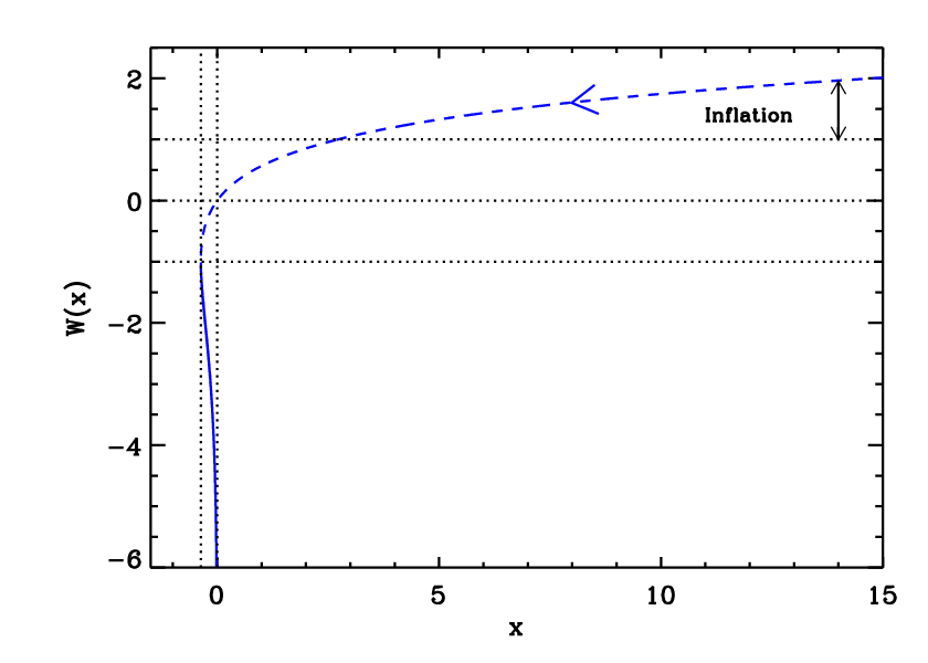
Refer to caption
Figure 12: Lambert functions W0​(x)\mathrm{W}_{\negthinspace 0}(x) (dashed line) and W−1​(x)\mathrm{W}_{\negthinspace-1}(x) (solid line). During Mixed Large Field inflation, inflation proceeds along the “00” branch above the line W=1W=1 in the direction specified by the arrow.

We have seen that, in MLFI, inflation stops by violation of the slow-roll condition. Let us therefore determine the corresponding vev of the field. The condition ϵ1=1\epsilon_{1}=1 leads to

α​xend3−2​2​α​xend2+xend−2=0.\alpha x_{\mathrm{end}}^{3}-2\sqrt{2}\alpha x_{\mathrm{end}}^{2}+x_{\mathrm{end}}-\sqrt{2}=0. (211)

This is a cubic algebraic equation that can be solved exactly. In the limit α≫1\alpha\gg 1, the solution reads xend≃2​2x_{\mathrm{end}}\simeq 2\sqrt{2} which is indeed the solution for the quartic case, see Eq. (197). On the other hand, if α≪1\alpha\ll 1, then xend≃2x_{\mathrm{end}}\simeq\sqrt{2} which is also the correct result for the quadratic case. The general solution is

xend\displaystyle x_{\mathrm{end}} =2​23+13​α​{14​2​[4​α2​(32​α+9)+2​α​4​α2​(32​α+9)2−8​α​(8​α−3)3]}1/3\displaystyle=\frac{2\sqrt{2}}{3}+\frac{1}{3\alpha}\Biggl\{\frac{1}{4\sqrt{2}}\Biggl[4\alpha^{2}\left(32\alpha+9\right)+2\alpha\sqrt{4\alpha^{2}\left(32\alpha+9\right)^{2}-8\alpha\left(8\alpha-3\right)^{3}}\Biggr]\Biggr\}^{1/3} (212)
+13(8α−3){14​2[4α2(32α+9)+2α4​α2​(32​α+9)2−8​α​(8​α−3)3]}−1/3,\displaystyle+\frac{1}{3}\left(8\alpha-3\right)\Biggl\{\frac{1}{4\sqrt{2}}\Biggl[4\alpha^{2}\left(32\alpha+9\right)+2\alpha\sqrt{4\alpha^{2}\left(32\alpha+9\right)^{2}-8\alpha\left(8\alpha-3\right)^{3}}\Biggr]\Biggr\}^{-1/3}\,,

which is the one used in the ASPIC library.

Finally, the parameter MM can be determined from the amplitude of the CMB anisotropies, and one gets

(MMPl)4=2880​π2x4​(1+2​α​x∗2)2(1+α​x∗2)3​Qrms−PS2T2.\left(\frac{M}{M_{\scriptscriptstyle{\mathrm{Pl}}}}\right)^{4}=\frac{2880\pi^{2}}{x^{4}}\frac{\left(1+2\alpha x_{*}^{2}\right)^{2}}{\left(1+\alpha x_{*}^{2}\right)^{3}}\frac{Q_{\mathrm{rms-PS}}^{2}}{T^{2}}\,. (213)

Similarly to LFI (see section 5.2), this gives rise to M/MPl≃10−3M/M_{\scriptscriptstyle{\mathrm{Pl}}}\simeq 10^{-3}. The reheating consistent slow-roll predictions for the MLFI models are displayed in Fig. 128. The reheating equation of state parameter w¯reh\overline{w}_{\mathrm{reh}} has been taken to 00 which is consistent with the fact that the potential is quadratic close to its minimum. As expected, when α≪1\alpha\ll 1 the predictions of the model match those of LFI with p=2p=2 and are aligned along the ϵ1=ϵ2/2\epsilon_{1}=\epsilon_{2}/2 line. On the other hand, if α≫1\alpha\gg 1, then the predictions are consistent with those of LFI with p=4p=4 and are aligned along the ϵ1=ϵ2\epsilon_{1}=\epsilon_{2} line. In the intermediate regime, it is interesting to notice that the MLFI predictions continuously interpolate between these two asymptotic solutions but do not remain inside the domain delimited by those two lines. Indeed, when α\alpha is larger than some value, one has ϵ1>ϵ2\epsilon_{1}>\epsilon_{2}. This means that, if one starts from a pure quartic potential (LFI with p=4p=4) and adds a small quadratic term, this extra term has the effect of increasing the “effective value” of pp, which is quite counter intuitive. On the other hand, since the quadratic model fits better the data than the quartic one, small values for the parameter α\alpha are favored (all the models with α>10−3\alpha>10^{-3} lie outside the 2​σ2\sigma contour of the Planck 2018 + Bicep-Keck data). High reheating temperatures are also preferred.

5.4 Radiatively Corrected Massive Inflation (RCMI)

Refer to caption
Refer to caption
Refer to caption
Refer to caption
Figure 13: Radiatively Corrected Massive Inflation (RCMI) for α=0.01\alpha=0.01. Top panels: potential (left) and logarithm of the potential (right). Bottom left panel: slow-roll parameter ϵ1\epsilon_{1} with respect to field values. The shaded area indicates where inflation stops. Bottom right panel: slow-roll parameters ϵ2\epsilon_{2} (solid line) and ϵ3\epsilon_{3} (dotted line).

This model is based on Ref. [310] and implements radiative corrections due to fermion couplings over the massive (p=2p=2) large field model (see section 5.2). With an appropriate choice of the renormalization scale μ=g​MPl\mu=gM_{\scriptscriptstyle{\mathrm{Pl}}}, gg denoting the Yukawa coupling, the potential is given by

V⁡(ϕ)\displaystyle V(\phi) =12​m2​ϕ2−g416​π2​ϕ4​ln⁡(ϕMPl)=M4​(ϕMPl)2​[1−2​α​ϕ2MPl2​ln⁡(ϕMPl)],\displaystyle=\frac{1}{2}m^{2}\phi^{2}-\frac{g^{4}}{16\pi^{2}}\phi^{4}\ln\left(\frac{\phi}{M_{\scriptscriptstyle{\mathrm{Pl}}}}\right)=M^{4}\left(\frac{\phi}{M_{\scriptscriptstyle{\mathrm{Pl}}}}\right)^{2}\left[1-2\alpha\frac{\phi^{2}}{M_{\scriptscriptstyle{\mathrm{Pl}}}^{2}}\ln\left(\frac{\phi}{M_{\scriptscriptstyle{\mathrm{Pl}}}}\right)\right], (214)

where

M4≡12​m2​MPl2,α≡g4​MPl216​π2​m2.M^{4}\equiv\dfrac{1}{2}m^{2}M_{\scriptscriptstyle{\mathrm{Pl}}}^{2},\qquad\alpha\equiv\frac{g^{4}M_{\scriptscriptstyle{\mathrm{Pl}}}^{2}}{16\pi^{2}m^{2}}\,. (215)

This expression is obtained in the large field regime ϕ≫m/g\phi\gg m/g (this condition coming from the requirement that the fermion loop contribution dominates over the self-interaction loop contribution), i.e. assuming that the inflationary regime takes place under the condition

ϕ4MPl4≫18​π2​α​M4MPl4.\dfrac{\phi^{4}}{M_{\scriptscriptstyle{\mathrm{Pl}}}^{4}}\gg\dfrac{1}{8\pi^{2}\alpha}\dfrac{M^{4}}{M_{\scriptscriptstyle{\mathrm{Pl}}}^{4}}\,. (216)

Defining x≡ϕ/MPlx\equiv\phi/M_{\scriptscriptstyle{\mathrm{Pl}}}, the Hubble flow functions are given by

ϵ1=2x2​(1−α​x2−4​α​x2​ln⁡x1−2​α​x2​ln⁡x)2,\displaystyle\epsilon_{1}=\dfrac{2}{x^{2}}\left(\frac{1-\alpha x^{2}-4\alpha x^{2}\ln x}{1-2\alpha x^{2}\ln x}\right)^{2}\,, (217)
ϵ2=4x2​(1+α​x2)​(1+2​α​x2)−2​α​x2​ln⁡x⁡(1−α​x2−4​α​x2​ln⁡x)(1−2​α​x2​ln⁡x)2,\displaystyle\epsilon_{2}=\dfrac{4}{x^{2}}\dfrac{\left(1+\alpha x^{2}\right)\left(1+2\alpha x^{2}\right)-2\alpha x^{2}\ln x\left(1-\alpha x^{2}-4\alpha x^{2}\ln x\right)}{\left(1-2\alpha x^{2}\ln x\right)^{2}}\,, (218)

and

ϵ3=4x2​1−α​x2−4​α​x2​ln⁡x(1−2​α​x2​ln⁡x)2\displaystyle\epsilon_{3}=\dfrac{4}{x^{2}}\dfrac{1-\alpha x^{2}-4\alpha x^{2}\ln x}{\left(1-2\alpha x^{2}\ln x\right)^{2}} (219)
×1−α​x2​[α​x2​(4​α​x2+9)+1]−α​x2​ln⁡x⁡[4​α2​x4​ln⁡x⁡(4​ln⁡x+1)+(α​x2+3)​(6​α​x2+2)](1+α​x2)​(1+2​α​x2)−2​α​x2​ln⁡x⁡(1−α​x2−4​α​x2​ln⁡x).\displaystyle\times\dfrac{1-\alpha x^{2}\left[\alpha x^{2}\left(4\alpha x^{2}+9\right)+1\right]-\alpha x^{2}\ln x\left[4\alpha^{2}x^{4}\ln x(4\ln x+1)+\left(\alpha x^{2}+3\right)\left(6\alpha x^{2}+2\right)\right]}{\left(1+\alpha x^{2}\right)\left(1+2\alpha x^{2}\right)-2\alpha x^{2}\ln x\left(1-\alpha x^{2}-4\alpha x^{2}\ln x\right)}\,.

If α=0\alpha=0, one recovers the slow-roll parameters of the massive case (namely LFI with p=2p=2, see section 5.2) as expected. The potential and Hubble-flow functions have been represented in Fig. 13.

Let us now discuss the field domains in which inflation can take place. It is clear that the above potential is not positive definite for all field values. It becomes negative at the point

xV=0=ϕV=0MPl=1α​W0​(1/α),x_{V=0}=\dfrac{\phi_{V=0}}{M_{\scriptscriptstyle{\mathrm{Pl}}}}=\sqrt{\frac{1}{\alpha\mathrm{W}_{\negthinspace 0}\left(1/\alpha\right)}}\,, (220)

where W0\mathrm{W}_{\negthinspace 0} is the 00-branch of the Lambert function. The model is defined only in the regime ϕ<ϕV=0\phi<\phi_{V=0}. On the other hand, the top of the potential, where V′=0V^{\prime}=0 (or equivalently ϵ1=0\epsilon_{1}=0), is given by

xtop=ϕtopMPl=12​α​W0​(e2​α).x_{\mathrm{top}}=\dfrac{\phi_{\mathrm{top}}}{M_{\scriptscriptstyle{\mathrm{Pl}}}}=\sqrt{\frac{1}{2\alpha\mathrm{W}_{\negthinspace 0}\left(\dfrac{\sqrt{e}}{2\alpha}\right)}}\,. (221)

As the model makes sense only if the logarithmic terms do not dominate the potential, the acceptable regime is ϕ<ϕtop<ϕV=0\phi<\phi_{\mathrm{top}}<\phi_{V=0}, and a large field region only exists for ϕtop/MPl≫1\phi_{\mathrm{top}}/M_{\scriptscriptstyle{\mathrm{Pl}}}\gg 1. From the above expression, this means that we must be in the regime α≪1\alpha\ll 1. For ϕ<ϕtop\phi<\phi_{\mathrm{top}} one can check from Eqs. (214) and (221) that the loop corrections never exceed α/e\alpha/e.

Let us now turn to the slow-roll trajectory. It is given by

N−Nend=−12∫ϕend/MPlϕ/MPlx−2​α​x3​ln⁡x1−α​x2−4​α​x2​ln⁡xdx,N-N_{\mathrm{end}}=-\frac{1}{2}\int_{\phi_{\mathrm{end}}/M_{\scriptscriptstyle{\mathrm{Pl}}}}^{\phi/M_{\scriptscriptstyle{\mathrm{Pl}}}}\frac{x-2\alpha x^{3}\ln x}{1-\alpha x^{2}-4\alpha x^{2}\ln x}\mathrm{d}x, (222)

an integral that cannot be performed analytically and which is numerically evaluated in ASPIC. For the purpose of this section, we can nevertheless make an expansion in α\alpha to obtain an approximate expression

N−Nend\displaystyle N-N_{\mathrm{end}} =−x24​[1+α​x24​(1+4​ln⁡x)]+xend24​[1+α​xend24​(1+4​ln⁡xend)]+𝒪⁡(α2).\displaystyle=-\dfrac{x^{2}}{4}\left[1+\alpha\dfrac{x^{2}}{4}\left(1+4\ln x\right)\right]+\dfrac{x_{\mathrm{end}}^{2}}{4}\left[1+\alpha\dfrac{x_{\mathrm{end}}^{2}}{4}\left(1+4\ln x_{\mathrm{end}}\right)\right]+\mathcal{O}\!\left(\alpha^{2}\right)\,. (223)

Inflation stops close to the minimum of the potential when ϵ1=1\epsilon_{1}=1. This last equation cannot be solved analytically but we can also perform an expansion at first order in α\alpha and one gets

xend=ϕendMPl≃12​α​W0​[e1+1/(4​α)2​α]≃2−2​2​α.x_{\mathrm{end}}=\frac{\phi_{\mathrm{end}}}{M_{\scriptscriptstyle{\mathrm{Pl}}}}\simeq\dfrac{1}{\sqrt{2\alpha\mathrm{W}_{\negthinspace 0}\left[\dfrac{e^{1+1/(4\alpha)}}{2\alpha}\right]}}\simeq\sqrt{2}-2\sqrt{2}\alpha\,. (224)

In the limit α→0\alpha\rightarrow 0, we recover the large field result for p=2p=2, i.e. xend→2x_{\mathrm{end}}\rightarrow\sqrt{2}. The maximum total number of ee-folds one can realize between ϕ=ϕtop\phi=\phi_{\mathrm{top}} and ϕ=ϕend\phi=\phi_{\mathrm{end}} can be calculated from the previous expressions. It reads

Δ​Nmax=Nend−Ntop\displaystyle\Delta N_{\max}=N_{\mathrm{end}}-N_{\mathrm{top}} =532​α​W0​(e2​α)+1+2​α−20​α​W0​[e1+1/(4​α)2​α]128​α2​W02​[e1+1/(4​α)2​α]\displaystyle=\dfrac{5}{32\alpha\mathrm{W}_{\negthinspace 0}\left(\dfrac{\sqrt{e}}{2\alpha}\right)}+\dfrac{1+2\alpha-20\alpha\mathrm{W}_{\negthinspace 0}\left[\dfrac{e^{1+1/(4\alpha)}}{2\alpha}\right]}{128\alpha^{2}\mathrm{W}_{\negthinspace 0}^{2}\left[\dfrac{e^{1+1/(4\alpha)}}{2\alpha}\right]} (225)
≃−532​α​ln⁡(α).\displaystyle\simeq-\frac{5}{32\alpha\ln\left(\alpha\right)}\,.

This is a decreasing function of α\alpha, so that α\alpha has to be small enough if one wants a sufficiently high number of ee-folds to take place. Indeed, if one wants at least Δ​Nmin\Delta N_{\min} ee-folds to occur, one needs to work with

α<532​Δ​Nmin​1ln⁡(32​Δ​Nmin10).\alpha<\frac{5}{32\Delta N_{\min}}\frac{1}{\ln\left(\frac{32\Delta N_{\min}}{10}\right)}\,. (226)

For example, Δ​Nmin=50\Delta N_{\min}=50 imposes α<6×10⁻⁴\alpha<6\times 10^{-4}. The fact that α\alpha is bounded from above can be directly checked in Fig. 129. The field ϕ∗\phi_{*} value at which the pivot mode crossed the Hubble radius during inflation is obtained from Eq. (51) whereas the corresponding ee-fold number can be obtained from the trajectory.

Finally, the parameter MM can be determined from the amplitude of the CMB anisotropies, and one gets

(MMPl)4\displaystyle\left(\frac{M}{M_{\scriptscriptstyle{\mathrm{Pl}}}}\right)^{4} =2880​π2x∗4​(1−2​α​x∗2​ln⁡x∗)3(1−α​x∗2−4​α​x∗2​ln⁡x∗)2​Qrms−PS2T2.\displaystyle=\dfrac{2880\pi^{2}}{x_{*}^{4}}\dfrac{\left(1-2\alpha x_{*}^{2}\ln x_{*}\right)^{3}}{\left(1-\alpha x_{*}^{2}-4\alpha x_{*}^{2}\ln x_{*}\right)^{2}}\frac{Q_{\mathrm{rms-PS}}^{2}}{T^{2}}\,. (227)

The reheating consistent slow-roll predictions for the RCMI models are represented in Fig. 129. As expected, the LFI quadratic model case is properly recovered for α→0\alpha\rightarrow 0. From this figure, we see that all models having α≳10−3.7\alpha\gtrsim 10^{-3.7} lie outside the 2​σ2\sigma contour. Let us emphasize that the value of α\alpha cannot be infinitely small due to Eq. (216). At zero order, one has ϕ>ϕend≃2​MPl\phi>\phi_{\mathrm{end}}\simeq\sqrt{2}M_{\scriptscriptstyle{\mathrm{Pl}}} such that Eq. (216) can be recast into

α>M48​π2​MPl4=m216​π2​MPl2.\alpha>\dfrac{M^{4}}{8\pi^{2}M_{\scriptscriptstyle{\mathrm{Pl}}}^{4}}=\frac{m^{2}}{16\pi^{2}M_{\scriptscriptstyle{\mathrm{Pl}}}^{2}}\,. (228)

From the COBE normalization, and in the limit of small α\alpha, one gets M/MPl≳10−3M/M_{\scriptscriptstyle{\mathrm{Pl}}}\gtrsim 10^{-3} and the lower bound reads α>10−15\alpha>10^{-15}.

5.5 Radiatively Corrected Quartic Inflation (RCQI)

This model is similar to RCMI discussed in section 7.1 but implements radiative corrections due to fermion couplings over a quartic (p=4p=4) large field model [310] (see section 5.2). The potential is given by

V=λ​ϕ4−g416​π2​ϕ4​ln⁡(ϕMPl)=M4​(ϕMPl)4​[1−α​ln⁡(ϕMPl)],\displaystyle V=\lambda\phi^{4}-\frac{g^{4}}{16\pi^{2}}\phi^{4}\ln\left(\frac{\phi}{M_{\scriptscriptstyle{\mathrm{Pl}}}}\right)=M^{4}\left(\frac{\phi}{M_{\scriptscriptstyle{\mathrm{Pl}}}}\right)^{4}\left[1-\alpha\ln\left(\frac{\phi}{M_{\scriptscriptstyle{\mathrm{Pl}}}}\right)\right], (229)

where

M4=λ​MPl4,α≡g416​π2​λ.M^{4}=\lambda M_{\scriptscriptstyle{\mathrm{Pl}}}^{4},\qquad\alpha\equiv\frac{g^{4}}{16\pi^{2}\lambda}\,. (230)

Defining x=ϕ/MPlx=\phi/M_{\scriptscriptstyle{\mathrm{Pl}}}, the Hubble flow functions in the slow-roll approximation read

ϵ1=8x2(1−α4−α​ln⁡x1−α​ln⁡x)2,ϵ2=8x21+α4​(α−1)+α⁡(α4−2)​ln⁡x+α2​ln2​x(1−α​ln⁡x)2,\displaystyle\epsilon_{1}=\dfrac{8}{x^{2}}\left(\dfrac{1-\dfrac{\alpha}{4}-\alpha\ln x}{1-\alpha\ln x}\right)^{2},\qquad\epsilon_{2}=\frac{8}{x^{2}}\dfrac{1+\dfrac{\alpha}{4}(\alpha-1)+\alpha\left(\dfrac{\alpha}{4}-2\right)\ln x+\alpha^{2}\ln^{2}x}{\left(1-\alpha\ln x\right)^{2}}\,, (231)

and

ϵ3\displaystyle\epsilon_{3} =8x2​(1−α2−α​ln​x)​(1−α4−α​ln​x)​[1+α22+α4−α⁡(2+α4−α​ln​x)​ln​x](1−α​ln​x)2​[1+α4​(α−1)−α⁡(2−α4−α​ln​x)​ln​x].\displaystyle=\dfrac{8}{x^{2}}\frac{(1-\dfrac{\alpha}{2}-\alpha\ln x)(1-\dfrac{\alpha}{4}-\alpha\ln x)\left[1+\dfrac{\alpha^{2}}{2}+\dfrac{\alpha}{4}-\alpha\left(2+\dfrac{\alpha}{4}-\alpha\ln x\right)\ln x\right]}{(1-\alpha\ln x)^{2}\left[1+\dfrac{\alpha}{4}(\alpha-1)-\alpha\left(2-\dfrac{\alpha}{4}-\alpha\ln x\right)\ln x\right]}\,. (232)

The shape of the potential and the Hubble flow functions are very similar to the ones of the RCMI model and have been represented in Fig. 14.

Refer to caption
Refer to caption
Refer to caption
Refer to caption
Figure 14: Radiatively Corrected Quartic Inflation (RCQI) for α=0.8\alpha=0.8. Top panels: the potential and its logarithm as a function of the field values. Bottom left panel: slow-roll parameter ϵ1\epsilon_{1}. The shaded area indicates where inflation stops. Bottom right panel: slow-roll parameters ϵ2\epsilon_{2} (solid line) and ϵ3\epsilon_{3} (dotted line). The shaded region for ϵ2\epsilon_{2} and ϵ3\epsilon_{3} shows where the slow-roll approximation is violated for that value of α\alpha.

In particular, the potential is vanishing and maximal at the field values

xV=0=ϕV=0MPl=e1/α,xtop=ϕtopMPl=e1/α−1/4,x_{V=0}=\dfrac{\phi_{V=0}}{M_{\scriptscriptstyle{\mathrm{Pl}}}}=e^{1/\alpha},\quad x_{\mathrm{top}}=\dfrac{\phi_{\mathrm{top}}}{M_{\scriptscriptstyle{\mathrm{Pl}}}}=e^{1/\alpha-1/4}, (233)

respectively. As the model makes sense only if the corrections are small compared to the quartic term, one should consider α≪1\alpha\ll 1 and not too large super-Planckian field values.

The slow-roll trajectory can integrated analytically from Eqs. (14) and (229) and one gets

N−Nend=−116[\displaystyle N-N_{\mathrm{end}}=-\frac{1}{16}\Biggl[ 2x2−e−1/2+2/αEi(12−2α+2lnx)\displaystyle 2x^{2}-e^{-1/2+2/\alpha}\Ei\left(\frac{1}{2}-\frac{2}{\alpha}+2\ln x\right) (234)
−2xend2+e−1/2+2/αEi(12−2α+2lnxend)],\displaystyle-2x_{\mathrm{end}}^{2}+e^{-1/2+2/\alpha}\Ei\left(\frac{1}{2}-\frac{2}{\alpha}+2\ln x_{\mathrm{end}}\right)\Biggr],

where the exponential integral function is defined by

Ei(x)≡−∫−x+∞e−ttdt.\Ei(x)\equiv-\int_{-x}^{+\infty}\frac{e^{-t}}{t}\mathrm{d}t. (235)

The quartic limit α→0\alpha\rightarrow 0 is recovered by noticing that

Ei(−2/α)∼α→0−α2e−2/α.\Ei(-2/\alpha)\underset{\alpha\rightarrow 0}{\sim}-\dfrac{\alpha}{2}e^{-2/\alpha}. (236)

Contrary to the RCMI model, the top of the potential is flat enough to support inflation. Indeed, one sees from Eq. (233) that the argument of the exponential integral function vanishes at x=xtopx=x_{\mathrm{top}}. Since for y→0y\rightarrow 0, one has Ei⁡(y)∼γ+ln⁡y\Ei(y)\sim\gamma+\ln y, whatever the value of xendx_{\mathrm{end}} the total number of ee-folds is divergent. This means that it is always possible to realize the required Δ​N∗\Delta N_{*} number of ee-folds provided inflation starts close enough to the top of the potential.

As for RCMI, inflation stops at ϵ1=1\epsilon_{1}=1 but this equation can only be solved numerically. For illustrative purpose, one can nevertheless solve it at first order in α\alpha to get

xend=ϕendMPl≃2​2−22​α.x_{\mathrm{end}}=\frac{\phi_{\mathrm{end}}}{M_{\scriptscriptstyle{\mathrm{Pl}}}}\simeq 2\sqrt{2}-\frac{\sqrt{2}}{2}\alpha. (237)

The link between ϕ∗\phi_{*} and Δ​N∗\Delta N_{*} is given by the slow-roll trajectory with ϕ∗\phi_{*} given by Eq. (51).

Finally, the parameter MM can be determined from the amplitude of the CMB anisotropies, and one gets

λ=M4MPl4=11520​π2x∗6​(1−α4−α​ln⁡x∗)2(1−α​ln⁡x∗)3​Qrms−PS2T2.\lambda=\frac{M^{4}}{M_{\scriptscriptstyle{\mathrm{Pl}}}^{4}}=\dfrac{11520\pi^{2}}{x_{*}^{6}}\dfrac{\left(1-\frac{\alpha}{4}-\alpha\ln x_{*}\right)^{2}}{\left(1-\alpha\ln x_{*}\right)^{3}}\frac{Q_{\mathrm{rms-PS}}^{2}}{T^{2}}\,. (238)

The slow-roll predictions for RCQI are represented in Fig. 130 and 131. As expected, the quartic model case is properly recovered in the limit α→0\alpha\rightarrow 0. From Fig. 130, we see that all the models seem to lie outside the 2​σ2\sigma contour for w¯reh=0\overline{w}_{\mathrm{reh}}=0. As the reheating phase takes place at the bottom of a quartic-like potential, we have also represented the prediction for w¯reh=1/3\overline{w}_{\mathrm{reh}}=1/3 in Fig. 131. For a radiation-dominated reheating, Δ​N∗\Delta N_{*} is fixed and for each value of α\alpha one has only a single point. In that situation, all these models are still disfavored at the two-sigma level.

5.6 Natural Inflation (NI)

5.6.1 Theoretical Justifications

Natural inflation was first proposed as an attempt to solve the so-called “fine-tuning” problem of inflation. In particular, in order to obtain sufficient inflation and the correct normalization for the microwave background anisotropies, the potential V⁡(ϕ)V(\phi) of the inflaton must be sufficiently flat. It is usually argued that, on general grounds, such a flatness is not robust under radiative corrections, unless it is protected by some symmetry. This is the reason that has motivated Refs. [311, 312] to put forward Natural Inflation, in which the inflaton potential is flat due to shift symmetries. The model makes use of Nambu-Goldstone bosons [313, 314] which arise whenever a global symmetry is spontaneously broken. The main idea can be very simply illustrated with the following action

S\displaystyle S =\displaystyle= −∫d𝒙−g[gμ​ν∂μΦ†∂νΦ+iΨ¯γμ∂μΨ+λ(Φ†Φ−f22)2\displaystyle-\int\mathrm{d}{\boldsymbol{x}}\sqrt{-g}\biggl[g^{\mu\nu}\partial_{\mu}\Phi^{\dagger}\partial_{\nu}\Phi+i\bar{\Psi}\gamma^{\mu}\partial_{\mu}\Psi+\lambda\left(\Phi^{\dagger}\Phi-\frac{f^{2}}{2}\right)^{2} (239)
+gfΨ¯LΦΨR+gfΨ¯RΦ†ΨL],\displaystyle+g_{\mathrm{f}}\bar{\Psi}_{\mathrm{L}}\Phi\Psi_{\mathrm{R}}+g_{\mathrm{f}}\bar{\Psi}_{\mathrm{R}}\Phi^{\dagger}\Psi_{\mathrm{L}}\biggr],

where Φ\Phi is a complex scalar field, Ψ\Psi a Dirac spinor and ΨLR=(1±γ5)/2​Ψ\Psi_{\mathrm{L}\mathrm{R}}=\left(1\pm\gamma_{5}\right)/2\Psi. The quantity ff is the energy scale at which the symmetry is spontaneously broken, λ\lambda is a dimensionless coupling constant and gfg_{\mathrm{f}} a dimensionless Yukawa coupling. This action is invariant under the U⁡(1)\mathrm{U}(1) transformation: Φ→ei​α​Φ\Phi\rightarrow e^{i\alpha}\Phi, ΨL→ei​α/2​ΨL\Psi_{\mathrm{L}}\rightarrow e^{i\alpha/2}\Psi_{\mathrm{L}} and ΨR→e−iα/2ΨR\Psi_{\mathrm{R}}\rightarrow e^{-i\alpha/2}\Psi_{\mathrm{R}}, where α\alpha is an arbitrary constant. Due to the “Mexican hat” potential for the scalar field, this symmetry is spontaneously broken below the scale ff and the scalar field acquires the vev ⟨Φ⟩=f/2​ei​ϕ/f\langle\Phi\rangle=f/\sqrt{2}e^{i\phi/f}. The field ϕ\phi corresponds to an “angular variable” and is a Goldstone boson. Below the scale of broken symmetry, the effective Lagrangian can be expressed as

ℒ=12∂μϕ∂μϕ+iΨ¯γμ∂μΨ+gff2(Ψ¯LΨRei​ϕ/f+Ψ¯RΨLe−iϕ/f).\mathcal{L}=\frac{1}{2}\partial_{\mu}\phi\partial^{\mu}\phi+i\bar{\Psi}\gamma^{\mu}\partial_{\mu}\Psi+g_{\mathrm{f}}\frac{f}{\sqrt{2}}\left(\bar{\Psi}_{\mathrm{L}}\Psi_{\mathrm{R}}e^{i\phi/f}+\bar{\Psi}_{\mathrm{R}}\Psi_{\mathrm{L}}e^{-i\phi/f}\right). (240)

It is now invariant under ϕ→ϕ+2​π​f\phi\rightarrow\phi+2\pi f, ΨL→ei​α/2​ΨL\Psi_{\mathrm{L}}\rightarrow e^{i\alpha/2}\Psi_{\mathrm{L}} and ΨR→e−iα/2ΨR\Psi_{\mathrm{R}}\rightarrow e^{-i\alpha/2}\Psi_{\mathrm{R}}. Then, we assume that an explicit symmetry breaking takes place, for instance through the appearance of a fermion condensate for which ⟨Ψ¯​Ψ⟩≃Ms3\langle\bar{\Psi}\Psi\rangle\simeq M_{\mathrm{s}}^{3} where Ms<fM_{\mathrm{s}}<f is the scale at which this symmetry breaking occurs. As a consequence, the effective Lagrangian takes the form

ℒ=12​∂μϕ​∂μϕ+2​gf​Ms3​f2​cos⁡(ϕf).\mathcal{L}=\frac{1}{2}\partial_{\mu}\phi\partial^{\mu}\phi+2g_{\mathrm{f}}M_{\mathrm{s}}^{3}\frac{f}{\sqrt{2}}\cos\left(\frac{\phi}{f}\right). (241)

We see that the Nambu-Goldstone boson has acquired a cosine potential and the overall scale of the potential is given by M4≃gf​Ms3​fM^{4}\simeq g_{\mathrm{f}}M_{\mathrm{s}}^{3}f. Therefore, if one takes f≃MPlf\simeq M_{\scriptscriptstyle{\mathrm{Pl}}}, MsM_{\mathrm{s}} slightly below the GUT scale and a Yukawa coupling of order one, one can “naturally” generate a small ratio M/fM/f. A last remark is in order on this model. Suppose that quantum gravity effects generate non-renormalizable higher order terms in the action (239) like

ΔV=am​n|Φ|2​mMPl2​m+n−4(Φn+Φ†)n,\Delta V=a_{mn}\frac{|\Phi|^{2m}}{M_{\scriptscriptstyle{\mathrm{Pl}}}^{2m+n-4}}\left(\Phi^{n}+\Phi^{\dagger}{}^{n}\right), (242)

where am​na_{mn} are a priori unknown coefficients. After symmetry breaking, one would therefore obtain a correction of the form

Δ​V=am​n​MPl4​(fMPl)2​m+n​cos⁡(n​ϕf).\Delta V=a_{mn}M_{\scriptscriptstyle{\mathrm{Pl}}}^{4}\left(\frac{f}{M_{\scriptscriptstyle{\mathrm{Pl}}}}\right)^{2m+n}\cos\left(n\frac{\phi}{f}\right). (243)

If f≳MPlf\gtrsim M_{\scriptscriptstyle{\mathrm{Pl}}}, as favored by current cosmological data (see below) these terms should dominate unless the coefficients am​na_{mn} are fine-tuned to very small values. Notice that the overall scale of the potential is now given by am​n​MPl4a_{mn}M_{\scriptscriptstyle{\mathrm{Pl}}}^{4}, which also demands that am​n≲10−15a_{mn}\lesssim 10^{-15} in order to have the correct CMB normalization. These terms are therefore dangerous for the consistency and the natural character of the model. This model has been studied in more details in Refs. [315, 316, 317, 318, 319, 320, 321, 322, 323, 324, 325, 326, 327, 328, 329].

Many other types of candidates have subsequently been explored in order to produce scenarios similar to that of Natural Inflation. For example, in Ref. [330], it was suggested to use a pseudo-Nambu Goldstone boson as the rolling field in double field inflation. Then, NI potentials generated by radiative corrections in models with explicitly broken Abelian [331] and non-Abelian [332, 333] symmetries were considered, showing that NI models with f≃MPlf\simeq M_{\scriptscriptstyle{\mathrm{Pl}}} and f≪MPlf\ll M_{\scriptscriptstyle{\mathrm{Pl}}} can both be generated. In Refs. [334], the field ϕ\phi is considered to be a Polonyi field [335] and the model predicts that f=MPlf=M_{\scriptscriptstyle{\mathrm{Pl}}}. Refs. [336, 337] have examined natural inflation in the context of extra dimensions and Ref. [338] has used pseudo-Nambu Goldstone bosons from little Higgs models to drive hybrid inflation. Also, Refs. [339, 340] have used the natural inflation idea of pseudo-Nambu Goldstone bosons in the context of braneworld scenarios to drive inflation, Ref. [341] has studied the model in 5-DD warped backgrounds. The same potential has also been obtained and studied in Ref. [342] when studying instantons in non-linear sigma models, and in Ref. [343] as providing quintessential inflation. In some of these references the potential is sometimes found with the minus sign in front of the cosine term, which is, up to a shift in the field vev ϕ/f→ϕ/f+π\phi/f\rightarrow\phi/f+\pi, the same potential as already studied before. This last model has also been derived and studied in Refs. [336, 337, 344] in the context of orbifold GUT inflation, where the potential is given by

V⁡(ϕ)=M4​[F⁡(ϕϕ0)+F⁡(2​ϕϕ0)+F⁡(0)2],V(\phi)=M^{4}\left[F\left(\frac{\phi}{\phi_{{}_{0}}}\right)+F\left(2\frac{\phi}{\phi_{{}_{0}}}\right)+\frac{F(0)}{2}\right], (244)

with

F(x)=−∑n=1∞cos⁡(n​π​x)n5.F(x)=-\sum_{n=1}^{\infty}\frac{\cos\left(n\pi x\right)}{n^{5}}\,. (245)

This potential must be studied in its increasing branch, and in the small field limit. At leading order, one recovers the cosine potential.

Finally, an important question is whether a situation where f>MPlf>M_{\scriptscriptstyle{\mathrm{Pl}}} makes sense from the high energy physics and effective field theory point of view. In fact, it was shown in Refs. [345, 346, 347] that f⪅1012​GeVf\lessapprox 10^{12}\mathrm{GeV} in order for the corresponding energy density not to exceed the critical energy density. But this constraint applies to the post inflationary Universe and, during inflation, Ref. [348] has argued that it is not relevant. However, it remains the question of whether f>MPlf>M_{\scriptscriptstyle{\mathrm{Pl}}} makes sense or not. To address this issue, an interesting mechanism has been proposed in Ref. [349] (see also Ref. [350]) which shows that two axion fields at sub-Planckian scales can have an effective dynamics similar to the one field Natural Inflation model with f>MPlf>M_{\scriptscriptstyle{\mathrm{Pl}}}.

Let us consider a model with two axions, θ\theta and ρ\rho the effective Lagrangian of which is given by

ℒ=12​∂μθ​∂μθ+12​∂μρ​∂μρ+M14​[1−cos⁡(θf+ρg1)]+M24​[1−cos⁡(θf+ρg2)],\mathcal{L}=\frac{1}{2}\partial_{\mu}\theta\partial^{\mu}\theta+\frac{1}{2}\partial_{\mu}\rho\partial^{\mu}\rho+M_{1}^{4}\left[1-\cos\left(\frac{\theta}{f}+\frac{\rho}{g_{1}}\right)\right]+M_{2}^{4}\left[1-\cos\left(\frac{\theta}{f}+\frac{\rho}{g_{2}}\right)\right], (246)

where M1M_{1} and M2M_{2}, ff, g1g_{1} and g2g_{2} are constant, a priori, arbitrary scales. The same model can be re-written in terms of the fields ψ\psi and ξ\xi defined by

ψ=f​g1f2+g12​(θf+ρg1),ξ=f​g1f2+g12​(−θg1+ρf).\psi=\frac{fg_{1}}{\sqrt{f^{2}+g_{1}^{2}}}\left(\frac{\theta}{f}+\frac{\rho}{g_{1}}\right),\qquad\xi=\frac{fg_{1}}{\sqrt{f^{2}+g_{1}^{2}}}\left(-\frac{\theta}{g_{1}}+\frac{\rho}{f}\right). (247)

It is easy to show that this leads to

ℒ\displaystyle\mathcal{L} =\displaystyle= 12​∂μψ​∂μψ+12​∂μξ​∂μξ+M14​[1−cos⁡(f2+g12f​g1​ψ)]\displaystyle\frac{1}{2}\partial_{\mu}\psi\partial^{\mu}\psi+\frac{1}{2}\partial_{\mu}\xi\partial^{\mu}\xi+M_{1}^{4}\left[1-\cos\left(\frac{\sqrt{f^{2}+g_{1}^{2}}}{fg_{1}}\psi\right)\right] (248)
+M24​[1−cos⁡(f2+g1​g2f​g2​f2+g12​ψ+g1−g2g2​f2+g12​ξ)].\displaystyle+M_{2}^{4}\left[1-\cos\left(\frac{f^{2}+g_{1}g_{2}}{fg_{2}\sqrt{f^{2}+g_{1}^{2}}}\psi+\frac{g_{1}-g_{2}}{g_{2}\sqrt{f^{2}+g_{1}^{2}}}\xi\right)\right].

Moreover, the mass of the two fields ψ\psi and ξ\xi can be expressed as

mψ2=(1f2+1g12)​M14,mξ2=(g1−g2)2g22​(f2+g12)​M24.m_{\psi}^{2}=\left(\frac{1}{f^{2}}+\frac{1}{g_{1}^{2}}\right)M_{1}^{4},\qquad m_{\xi}^{2}=\frac{(g_{1}-g_{2})^{2}}{g_{2}^{2}\left(f^{2}+g_{1}^{2}\right)}M_{2}^{4}. (249)

If g1g_{1} is very close to g2g_{2}, then the field ξ\xi will be light and, therefore, will have a non-trivial dynamics. In addition, if the field ψ\psi is sufficiently heavy (compared to the Hubble parameter), then its vev will be frozen at ψ=0\psi=0. In this case, we see that the original two fields model effectively reduces to a one field NI model with a scale fξf_{\xi} given by

fξ=g2​f2+g12g1−g2.f_{\xi}=\frac{g_{2}\sqrt{f^{2}+g_{1}^{2}}}{g_{1}-g_{2}}. (250)

But, since, g1g_{1} is close to g2g_{2}, the scale fξf_{\xi} will be large even if the fundamental scales ff, g1g_{1} and/or g2g_{2} are sub-Planckian. In this way, one can generate super-Planckian values for the scale ff and, at the same time, have a theory which can be consistent from the effective field theory point of view.

Refer to caption
Refer to caption
Refer to caption
Refer to caption
Figure 15: Natural Inflation (NI). Top left panel: potential for f/MPl=1.5f/M_{\scriptscriptstyle{\mathrm{Pl}}}=1.5. Top right panel: logarithm of the potential for the same value of ff. Bottom left panel: slow-roll parameter ϵ1\epsilon_{1} for a potential with f/MPl=1.5f/M_{\scriptscriptstyle{\mathrm{Pl}}}=1.5. The shaded area indicates the breakdown of the slow-roll inflation (strictly speaking when the acceleration stops). Bottom right panel: slow-roll parameters ϵ2\epsilon_{2} (solid line) and ϵ3\epsilon_{3} (dotted line) for a potential with f/MPl=1.5f/M_{\scriptscriptstyle{\mathrm{Pl}}}=1.5.

5.6.2 Slow-Roll Analysis

Summarizing the above discussion, the model that we consider in this section makes use of a potential that can be written as

V⁡(ϕ)=M4​[1+cos⁡(ϕf)].V(\phi)=M^{4}\left[1+\cos\left(\frac{\phi}{f}\right)\right]. (251)

The scale MM is determined by the CMB normalization and the potential depends on one parameter: the a priori unknown scale ff. The potential of Eq. (251) is displayed with its logarithm in Fig. 15. Since it is a periodic and even function of the field vev ϕ\phi, it is enough to study it in the range ϕ∈[0,π​f]\phi\in[0,\pi f] where inflation proceeds from the left to the right. If one lets x≡ϕ/fx\equiv\phi/f, the slow-roll parameters can be expressed as

ϵ1=MPl22​f2​sin2⁡x(1+cos⁡x)2,ϵ2=2​MPl2f2​11+cos⁡x,ϵ3=2​ϵ1.\epsilon_{1}=\frac{M_{\scriptscriptstyle{\mathrm{Pl}}}^{2}}{2f^{2}}\frac{\sin^{2}x}{\left(1+\cos x\right)^{2}}\,,\qquad\epsilon_{2}=\frac{2M_{\scriptscriptstyle{\mathrm{Pl}}}^{2}}{f^{2}}\frac{1}{1+\cos x}\,,\qquad\epsilon_{3}=2\epsilon_{1}\,. (252)

They are displayed in Fig. 15, where one can see that they are all increasing functions of the field vev, which means that they all increase during inflation. Inflation stops at the position xendx_{\mathrm{end}} given by ϵ1=1\epsilon_{1}=1 (see below), and one can see that ϵ2\epsilon_{2} and ϵ3\epsilon_{3} are already greater than one at this point. This means that the slow-roll approximation stops being valid slightly before the end of inflation, and the few last ee-folds may not be properly described in this frame of approximations. Another remark to be made is the fact that one generically has

ϵ2>MPl2f2.\epsilon_{2}>\frac{M_{\scriptscriptstyle{\mathrm{Pl}}}^{2}}{f^{2}}\,. (253)

This means that in order for the slow-roll approximation to be valid, one must require f/MPl≫1f/M_{\scriptscriptstyle{\mathrm{Pl}}}\gg 1 which is not necessarily problematic from a high energy physics point of view (see the above discussion).

The end of inflation occurs when ϵ1=1\epsilon_{1}=1, i.e. at a position given by

xend=arccos⁡(1−2​f2/MPl21+2​f2/MPl2).x_{\mathrm{end}}=\arccos\left(\frac{1-2f^{2}/M_{\scriptscriptstyle{\mathrm{Pl}}}^{2}}{1+2f^{2}/M_{\scriptscriptstyle{\mathrm{Pl}}}^{2}}\right). (254)

From this expression, one can calculate the value of the other slow roll parameters at the end of inflation, namely ϵ2end=2+MPl2/f2\epsilon_{2}^{\mathrm{end}}=2+M_{\scriptscriptstyle{\mathrm{Pl}}}^{2}/f^{2} and ϵ3end=2​ϵ2end\epsilon_{3}^{\mathrm{end}}=2\epsilon_{2}^{\mathrm{end}}, which confirms that the last few ee-folds may not be described properly in the slow-roll approximation.

Let us now calculate the slow-roll trajectory. It is given by

Nend−N=f2MPl2​ln⁡(1−cos⁡xend1−cos⁡x),N_{\mathrm{end}}-N=\frac{f^{2}}{M_{\scriptscriptstyle{\mathrm{Pl}}}^{2}}\ln\left(\frac{1-\cos x_{\mathrm{end}}}{1-\cos x}\right), (255)

where NendN_{\mathrm{end}} is the number of ee-folds at the end of inflation, and NN is the number of ee-folds at some point when the scaled field vev is xx. This trajectory can be inverted and one obtains

x=arccos⁡{1−(1−cos⁡xend)​exp⁡[−MPl2f2​(Nend−N)]}.x=\arccos\left\{1-\left(1-\cos x_{\mathrm{end}}\right)\exp\left[-\frac{M_{\scriptscriptstyle{\mathrm{Pl}}}^{2}}{f^{2}}\left(N_{\mathrm{end}}-N\right)\right]\right\}\,. (256)

Replacing xendx_{\mathrm{end}} by its value [see Eq. (254)] gives

x=arccos⁡{1−4​f2MPl2+2​f2​exp⁡[−MPl2f2​(Nend−N)]}.x=\arccos\left\{1-\frac{4f^{2}}{M_{\scriptscriptstyle{\mathrm{Pl}}}^{2}+2f^{2}}\exp\left[-\frac{M_{\scriptscriptstyle{\mathrm{Pl}}}^{2}}{f^{2}}\left(N_{\mathrm{end}}-N\right)\right]\right\}\,. (257)

Finally, the amplitude of the CMB anisotropies fixes the parameter MM to

(MMPl)4=720​π2​Qrms−PS2T2​MPl2f2​sin2⁡x∗(1+cos⁡x∗)3.\left(\frac{M}{M_{\scriptscriptstyle{\mathrm{Pl}}}}\right)^{4}=720\pi^{2}\frac{Q_{\mathrm{rms-PS}}^{2}}{T^{2}}\frac{M_{\scriptscriptstyle{\mathrm{Pl}}}^{2}}{f^{2}}\frac{\sin^{2}x_{*}}{\left(1+\cos x_{*}\right)^{3}}\,. (258)

If f/MPl=𝒪⁡(1)f/M_{\scriptscriptstyle{\mathrm{Pl}}}=\mathcal{O}\!\left(1\right), this expression simplifies to

(MMPl)4≃720​π2​Qrms−PS2T2​e−2MPl2/f2ΔN∗1+2​f2/MPl2,\left(\frac{M}{M_{\scriptscriptstyle{\mathrm{Pl}}}}\right)^{4}\simeq 720\pi^{2}\frac{Q_{\mathrm{rms-PS}}^{2}}{T^{2}}\frac{e^{-2M_{\scriptscriptstyle{\mathrm{Pl}}}^{2}/f^{2}\Delta N_{*}}}{1+2f^{2}/M_{\scriptscriptstyle{\mathrm{Pl}}}^{2}}\,, (259)

which gives rise to M/MPl≃10−13M/M_{\scriptscriptstyle{\mathrm{Pl}}}\simeq 10^{-13}. On the contrary, if f/MPl≫1f/M_{\scriptscriptstyle{\mathrm{Pl}}}\gg 1 one has

(MMPl)4≃360​π2​Qrms−PS2T2​(fMPl)2​1Δ​N∗2,\left(\frac{M}{M_{\scriptscriptstyle{\mathrm{Pl}}}}\right)^{4}\simeq 360\pi^{2}\frac{Q_{\mathrm{rms-PS}}^{2}}{T^{2}}\left(\frac{f}{M_{\scriptscriptstyle{\mathrm{Pl}}}}\right)^{2}\frac{1}{\Delta N_{*}^{2}}\,, (260)

and the potential energy scale goes up. For instance, if f/MPl=102f/M_{\scriptscriptstyle{\mathrm{Pl}}}=10^{2} one has M/MPl≃10−2M/M_{\scriptscriptstyle{\mathrm{Pl}}}\simeq 10^{-2}.

The reheating consistent slow-roll predictions for the natural inflation models are displayed in Fig. 132. The reheating equation of state parameter w¯reh\overline{w}_{\mathrm{reh}} has been taken to 00 since the potential is quadratic close to its minimum. In the limit f/MPl→∞f/M_{\scriptscriptstyle{\mathrm{Pl}}}\rightarrow\infty, the quadratic model predictions (LFI with p=2p=2, see section 5.2) seem to be recovered. Indeed, from the above formula, one can check that in this limit both xendx_{\mathrm{end}} and x∗x_{*} approach π\pi and the potential is, at leading order, a parabola. More precisely, one can check from Eq. (257) that in the limit f/MPl→∞f/M_{\scriptscriptstyle{\mathrm{Pl}}}\rightarrow\infty, one has cos⁡x∗≃−1+(1+2​Δ​N∗)​MPl2/f2\cos x_{*}\simeq-1+\left(1+2\Delta N_{*}\right)M_{\scriptscriptstyle{\mathrm{Pl}}}^{2}/f^{2}, from which one deduces that ϵ1∗≃1/(1+2ΔN∗)\epsilon_{1*}\simeq 1/\left(1+2\Delta N_{*}\right) and ϵ2∗≃2/(1+2ΔN∗)≃2ϵ1∗\epsilon_{2*}\simeq 2/\left(1+2\Delta N_{*}\right)\simeq 2\epsilon_{1*}. These relations are characteristic of the LFI quadratic models, see Eq. (201). However, one has ϵ3∗=2ϵ2∗\epsilon_{3*}=2\epsilon_{2*} which differs from the LFI quadratic relationship ϵ3∗=ϵ2∗\epsilon_{3*}=\epsilon_{2*}, and therefore quantities sensitive to ϵ3\epsilon_{3}, such as the running αS\alpha_{\scriptscriptstyle{\mathrm{S}}}, would break the degeneracy between NI and the LFI quadratic model. As expected, large values of f/MPlf/M_{\scriptscriptstyle{\mathrm{Pl}}} seem to be favored by the data (as well as high reheating temperatures), and in practice, f/MPl<4f/M_{\scriptscriptstyle{\mathrm{Pl}}}<4 appears to be disfavored at the 2​σ2\sigma level by the Planck 2018 + Bicep-Keck data.

5.7 Exponential SUSY Inflation (ESI)

5.7.1 Theoretical Justifications

This model has been discussed in Ref. [351] in the context of spin-driven inflation and derived in Ref. [352] in the context of supergravity and superstrings. The potential is given by V(ϕ)∝(1−e−qϕ/MPl)V(\phi)\propto\left(1-e^{-q\phi/M_{\scriptscriptstyle{\mathrm{Pl}}}}\right). The same potential also appears in Ref. [353] in the context of brane inflation, in Ref. [354] in the context of type IIB string compactification as fibre inflation and more recently in Ref. [355] as unitarized Higgs inflation models. This type of models can be obtained under very general considerations. Suppose that one has a supergravity model with a Kähler potential depending on one field ψ\psi given by K=−β/κln(1−ακψψ†)K=-\beta/\kappa\ln\left(1-\alpha\kappa\psi\psi^{\dagger}\right), where α\alpha and β\beta are two free parameters. This model leads to a scalar potential but for a field which is not canonically normalized. The canonically normalized field θ\theta is given by

κ1/2​θ≃1α​(1−2​e−2/β​κ1/2​ψ),\kappa^{1/2}\theta\simeq\frac{1}{\sqrt{\alpha}}\left(1-2e^{-\sqrt{2/\beta}\kappa^{1/2}\psi}\right), (261)

where we have assumed that inflation takes place at relatively large ψ\psi vev’s. Then, suppose that the superpotential leads to a given function V=f⁡(θ)V=f(\theta). One can always expand ff such that

V⁡(ϕ)≃V0​(1−e−2/β​κ1/2​ϕ)+⋯,V(\phi)\simeq V_{0}\left(1-e^{-\sqrt{2/\beta}\kappa^{1/2}\phi}\right)+\cdots, (262)

where κ1/2​ϕ≡κ1/2​θ+β/2​ln⁡[2​fθ/(α​f)]\kappa^{1/2}\phi\equiv\kappa^{1/2}\theta+\sqrt{\beta/2}\ln\left[2f_{\theta}/(\sqrt{\alpha}f)\right] and V0V_{0} is just the function ff evaluated at 1/α1/\sqrt{\alpha}. We see that one obtains exactly the ESI potential with q=2/βq=\sqrt{2/\beta}. Preferred choices for β\beta are β=1\beta=1 or β=3\beta=3 leading to q=2q=\sqrt{2} or q=2/3q=\sqrt{2/3}. In absence of any more further guidance, it seems reasonable to assume that β\beta, and hence qq, is just a number of order one.

Refer to caption
Refer to caption
Refer to caption
Refer to caption
Figure 16: Exponential SUSY Inflation (ESI) for q=0.1q=0.1. Top panels: the potential and its logarithm. Bottom left panel: slow-roll parameter ϵ1\epsilon_{1}. The shaded area indicates where acceleration stops. Bottom right panel: slow-roll parameters ϵ2\epsilon_{2} (solid line) and ϵ3\epsilon_{3} (dotted line). For those, the shaded region signals the breakdown of the slow-roll approximation but not necessarily the end of the accelerated expansion.

5.7.2 Slow-roll Analysis

Based on the previous considerations, we now study the following potential

V(ϕ)=M4(1−e−qϕ/MPl),V(\phi)=M^{4}\left(1-e^{-q\phi/M_{\scriptscriptstyle{\mathrm{Pl}}}}\right), (263)

where qq is a positive dimensionless parameter and inflation proceeds at decreasing field values in the region where ϕ/MPl>0\phi/M_{\scriptscriptstyle{\mathrm{Pl}}}>0. Defining x≡ϕ/MPlx\equiv\phi/M_{\scriptscriptstyle{\mathrm{Pl}}}, the Hubble flow functions in the slow-roll approximation read

ϵ1=q22​e−2​q​x(1−e−q​x)2,ϵ2=2​q2​e−q​x(1−e−q​x)2,ϵ3=q2​e−q​x​(1+e−q​x)(1−e−q​x)2.\epsilon_{1}=\frac{q^{2}}{2}\frac{e^{-2qx}}{\left(1-e^{-qx}\right)^{2}}\,,\qquad\epsilon_{2}=2q^{2}\frac{e^{-qx}}{\left(1-e^{-qx}\right)^{2}}\,,\qquad\epsilon_{3}=q^{2}\frac{e^{-qx}\left(1+e^{-qx}\right)}{\left(1-e^{-qx}\right)^{2}}\,. (264)

The potential and the Hubble flow functions with respect to the field values are represented in Fig. 16.

Refer to caption
Figure 17: Lambert functions W0​(x)\mathrm{W}_{\negthinspace 0}(x) (dashed line) and W−1​(x)\mathrm{W}_{\negthinspace-1}(x) (solid line). During Exponential SUSY inflation, inflation proceeds along the “−1-1” branch in the direction specified by the arrow on the figure.

The slow-roll trajectory can be integrated analytically from Eq. (14) and one finds

N−Nend=−eq​x−q​xq2+eq​xend−q​xendq2.N-N_{\mathrm{end}}=-\dfrac{e^{qx}-qx}{q^{2}}+\dfrac{e^{qx_{\mathrm{end}}}-qx_{\mathrm{end}}}{q^{2}}\,. (265)

This equation can also be inverted in terms of the Lambert function to get the field value in terms of the number of ee-folds:

x=q⁡(N−Nend)−eq​xend−q​xendq−1q​W−1​{−exp⁡[q2​(N−Nend)−(eq​xend−q​xend)]}.x=q(N-N_{\mathrm{end}})-\dfrac{e^{qx_{\mathrm{end}}}-qx_{\mathrm{end}}}{q}-\frac{1}{q}\mathrm{W}_{\negthinspace-1}\left\{-\exp\left[q^{2}(N-N_{\mathrm{end}})-(e^{qx_{\mathrm{end}}}-qx_{\mathrm{end}})\right]\right\}. (266)

The fact that one should choose the branch W−1\mathrm{W}_{\negthinspace-1} is justified below. The argument of the Lambert function is always negative as the exponential is always positive. Moreover, since xend>0x_{\mathrm{end}}>0 and N<NendN<N_{\mathrm{end}}, the maximal value of exponential argument is saturated for xend→0x_{\mathrm{end}}\rightarrow 0, i.e. for a Lambert function argument equals to −1/e-1/e. As the result the Lambert function argument varies, at most, in [−1/e,0][-1/e,0]. Finally, since x>0x>0, we see directly from Eq. (266) that the Lambert function values have to be negative thereby ensuring that inflation proceeds only along the “−1-1”-branch (see Fig. 17).

With such a potential, inflation ends naturally at ϵ1=1\epsilon_{1}=1, i.e. at the field value

xend=1q​ln⁡(1+q2).x_{\mathrm{end}}=\frac{1}{q}\ln\left(1+\frac{q}{\sqrt{2}}\right). (267)

From this equation and the trajectory, we have an explicit relation between the field value ϕ∗\phi_{*} at which the pivot mode crossed the Hubble radius during inflation and the corresponding ee-fold number Δ​N∗\Delta N_{*}.

Finally, the parameter MM can be determined from the amplitude of the CMB anisotropies, and one gets

(MMPl)4=720​q2​π2​e−2​q​x∗(1−e−q​x∗)3​Qrms−PS2T2,\left(\frac{M}{M_{\scriptscriptstyle{\mathrm{Pl}}}}\right)^{4}=720q^{2}\pi^{2}\dfrac{e^{-2qx_{*}}}{\left(1-e^{-qx_{*}}\right)^{3}}\frac{Q_{\mathrm{rms-PS}}^{2}}{T^{2}}\,, (268)

where the value of ϕ∗\phi_{*} (or Δ​N∗\Delta N_{*}) is obtained from Eq. (51). The reheating consistent slow-roll prediction for the exponential Susy models are represented in Figs. 133 and 134. In the limit q→0q\rightarrow 0, we recover the same prediction as a linear large field model. From Fig. 133, we see that all the models remains compatible with the current data. These figures correspond to w¯reh=0\overline{w}_{\mathrm{reh}}=0, but one could argue that w¯reh≳−1/3\overline{w}_{\mathrm{reh}}\gtrsim-1/3 make more sense if a parametric reheating would feel the linear shape of the potential. This quite extreme situation is represented in Fig. 134. In that case, the low reheating temperatures are clearly disfavored.

5.8 Power Law Inflation (PLI)

Refer to caption
Refer to caption
Refer to caption
Refer to caption
Figure 18: Power Law Inflation (PLI) for α=0.3\alpha=0.3. Top panels: power law potential (left) and its logarithm (right). Bottom left panel: slow-roll parameter ϵ1\epsilon_{1}. Bottom right panel: slow-roll parameters ϵ2=ϵ3=0\epsilon_{2}=\epsilon_{3}=0. On these plots, the shaded area indicates the region where slow-roll is violated.

These models refer to inflationary potentials of the form

V(ϕ)=M4e−αϕ/MPl,V(\phi)=M^{4}e^{-\alpha\phi/M_{\scriptscriptstyle{\mathrm{Pl}}}}\,, (269)

where α\alpha is a dimensionless parameter. They have been intensively studied since they lead to an exact inflationary dynamics, of the power law form, hence their name. Moreover, the power spectrum can also be determined exactly in this case. The background solution reads a∝(t/t0)2/α2a\propto(t/t_{0})^{2/\alpha^{2}} and ϕ=ϕ0+2MPl/αln(t/t0)\phi=\phi_{{}_{0}}+2M_{\scriptscriptstyle{\mathrm{Pl}}}/\alpha\ln\left(t/t_{0}\right) with t02=2MPl2/(α2M4)(6/α2−1)eαϕ0/MPlt_{0}^{2}=2M_{\scriptscriptstyle{\mathrm{Pl}}}^{2}/(\alpha^{2}M^{4})(6/\alpha^{2}-1)e^{\alpha\phi_{{}_{0}}/M_{\scriptscriptstyle{\mathrm{Pl}}}}. We see that we have inflation provided α∈[0,2]\alpha\in\left[0,\sqrt{2}\right].

This scenario was introduced in Ref. [356, 357] where the two point correlation function of the cosmological fluctuations was calculated for the first time (see also Refs. [358, 359]). The predictions of this model were recently compared to the Planck data in Ref. [360]. Soon after Ref. [357], it was also considered in Refs. [361, 362] but in the context of quintessence, i.e. for models of dark energy in which the energy density of the scalar field redshifts as a power law of the scale factor ρ∝a−q\rho\propto a^{-q}. In that case, one has α=q/2\alpha=\sqrt{q/2}. The same potential also arises in the case where large field inflation is considered (LFI, see section 5.2) but with a non-minimal coupling of the inflaton to the gravity sector, see Refs. [363, 364] (the exponential potential appears after the transformation to the Einstein frame). In Ref. [365], a cosmic no-hair theorem for Bianchi models was proven assuming that the potential of the inflaton is of the same type as in Eq. (269). It was shown that one must have 0<α<2/30<\alpha<\sqrt{2/3} so that the isotropic power law solution is the unique attractor for any initially expanding Bianchi type model (except type IX). In Ref. [366], the potential (269) has been studied in the Kantowski-Sachs metric, and it was found that the production of particles by the scalar field acts as viscous forces which enlarges the range of initial conditions leading to successful inflation. In Ref. [367], the nature of the potential V⁡(ϕ)V(\phi) relevant to having inflation in presence of a minimally coupled scalar field together with a causal viscous fluid was investigated. It was shown that this leads to an exponential potential. In Refs. [368, 369, 370], the exponential potential was used to describe the dynamics of a tachyonic matter field (i.e. with a non-minimal kinetic term). In Ref. [371], the general transformations that leave unchanged the form of the field equations for Bianchi V cosmologies were investigated, and it was found that they admit asymptotic stable points that lead to power law solutions of the type (269). In Ref. [372], inflation was studied in the context of M-theory on S1/ℤ2S^{1}/\mathbb{Z}_{2} via the non-perturbative dynamics of M5-branes. The open membrane instanton interactions between the branes give rise to potentials of the type (269). Within the same framework, Ref. [373] has discussed a realization of cascade inflation as assisted inflation built upon a succession of power law inflationary eras. Ref. [374] has used the exponential potential (269) in the context of Randall-Sandrum type II Braneworld model. Finally, the general dynamics of power law inflation was studied in detail in Refs. [356, 375, 376, 377, 378, 379, 380, 381, 382, 383], where various aspects of its phenomenology were highlighted.

The potential and its logarithm are displayed in Fig. 18. They are decreasing functions of the field, hence inflation proceeds from the left to the right. The slow-roll parameters take a simple form given by

ϵ1=α22,ϵi>1=0.\epsilon_{1}=\frac{\alpha^{2}}{2},\quad\epsilon_{i>1}=0. (270)

Since the first slow-roll parameter is constant, inflation cannot stop by slow-roll violation and one has to assume that, at some vev ϕend\phi_{\mathrm{end}}, a tachyonic instability is triggered. A priori, this means that the model has in fact an additional new free parameter. However, because the slow-roll parameters do not depend on ϕ\phi, as well as all the other properties of the inflationary dynamics (even when the slow-roll approximation is not satisfied, see below), the observational predictions of the model cannot depend on ϕend\phi_{\mathrm{end}} and this parameter turns out to be irrelevant.

The Hubble flow hierarchy being almost trivial, the exact dynamics of the model can be worked out even if the slow-roll approximation is violated. Indeed, let us first notice that the slow-roll trajectory can be explicitly integrated, and gives

ϕMPl=ϕendMPl+α⁡(N−Nend).\frac{\phi}{M_{\scriptscriptstyle{\mathrm{Pl}}}}=\frac{\phi_{\mathrm{end}}}{M_{\scriptscriptstyle{\mathrm{Pl}}}}+\alpha\left(N-N_{\mathrm{end}}\right). (271)

Then, one can remark that this trajectory is also a solution of the exact Klein-Gordon equation of motion, which reads in terms of the number of ee-folds NN,

H2​∂2ϕ∂N2+(3​H2+H​∂∂H∂N)​∂ϕ∂N+d​Vd​ϕ=0.H^{2}\frac{\partial^{2}\phi}{\partial N^{2}}+\left(3H^{2}+H\partial\dfrac{\partial H}{\partial N}\right)\dfrac{\partial\phi}{\partial N}+\dfrac{\mathrm{d}V}{\mathrm{d}\phi}=0. (272)

Indeed, the first term vanishes, and the second term requires

H2=V+ϕ˙2/23​MPl2=V+H22​(∂ϕ∂N)23​MPl2=V+H22​α2​MPl23​MPl2,H^{2}=\frac{V+\dot{\phi}^{2}/2}{3M_{\scriptscriptstyle{\mathrm{Pl}}}^{2}}=\dfrac{V+\dfrac{H^{2}}{2}\left(\dfrac{\partial\phi}{\partial N}\right)^{2}}{3M_{\scriptscriptstyle{\mathrm{Pl}}}^{2}}=\dfrac{V+\dfrac{H^{2}}{2}\alpha^{2}M_{\scriptscriptstyle{\mathrm{Pl}}}^{2}}{3M_{\scriptscriptstyle{\mathrm{Pl}}}^{2}}\,, (273)

from which one gets

H2=V3​MPl2​11−α2/6.H^{2}=\dfrac{V}{3M_{\scriptscriptstyle{\mathrm{Pl}}}^{2}}\dfrac{1}{1-\alpha^{2}/6}\,. (274)

From there, one can evaluate all terms in the Klein-Gordon equation, and verify that Eq. (271) is indeed a solution of Eq. (272). Since it is a second order differential equation, other solutions exist, but it can be shown [361, 362] that the exact solution is an attractor. Let us also notice that combining Eq. (274) with Eq. (271) gives rise to

H=Hend​(aenda)α2/2,H=H_{\mathrm{end}}\left(\dfrac{a_{\mathrm{end}}}{a}\right)^{\alpha^{2}/2}, (275)

which can be integrated and gives

a⁡(t)=aend​(ttend)2/α2.a(t)=a_{\mathrm{end}}\left(\frac{t}{t_{\mathrm{end}}}\right)^{2/\alpha^{2}}. (276)

One recovers the solution mentioned at the beginning of this section. Finally, the equation of state w=P/ρw=P/\rho can also be worked out exactly and one gets

w=−1+α23.w=-1+\frac{\alpha^{2}}{3}\,. (277)

Again, all the previous expressions are valid even if the slow-roll approximation is not satisfied. One can see that pure de Sitter corresponds to α=0\alpha=0. In this case the potential is constant, the equation of state is −1-1 and the scale factor expands exponentially.

Another nice feature of power-law inflation is that the spectrum of the perturbations can be computed exactly without relying on any approximation. Defining the parameter β≤−2\beta\leq-2 from α2/2=(β+2)/(β+1)\alpha^{2}/2=(\beta+2)/(\beta+1), the primordial scalar power spectrum is given by

𝒫ζ=H∗2π​ϵ1​(8​π​MPl2)​f​(β)​(kk∗)2​β+4,{\mathcal{P}}_{\zeta}=\frac{H_{*}^{2}}{\pi\epsilon_{1}(8\pi M_{\scriptscriptstyle{\mathrm{Pl}}}^{2})}f(\beta)\left(\frac{k}{k_{*}}\right)^{2\beta+4}, (278)

where

f⁡(β)≡1π​[(1+β)1+β21+β​Γ​(12+β)]2.f(\beta)\equiv\frac{1}{\pi}\left[\frac{(1+\beta)^{1+\beta}}{2^{1+\beta}}\Gamma\left(\frac{1}{2}+\beta\right)\right]^{2}. (279)

In particular, f⁡(β=−2)=1f(\beta=-2)=1. The power spectrum of gravitational waves can also be obtained remarking that we have μS=μT\mu_{\scriptscriptstyle{\mathrm{S}}}=\mu_{\scriptscriptstyle{\mathrm{T}}} for power law inflation. From

𝒫ζ=k38​π2​|μSa​ϵ1|2,𝒫h=2​k3π2​|μTa|2,{\mathcal{P}}_{\zeta}=\frac{k^{3}}{8\pi^{2}}\left|\frac{\mu_{\scriptscriptstyle{\mathrm{S}}}}{a\sqrt{\epsilon_{1}}}\right|^{2},\qquad{\mathcal{P}}_{h}=\frac{2k^{3}}{\pi^{2}}\left|\frac{\mu_{\scriptscriptstyle{\mathrm{T}}}}{a}\right|^{2}, (280)

one gets

r≡𝒫h𝒫ζ=16​ϵ1=16​nTnT−2,r\equiv\frac{{\mathcal{P}}_{h}}{{\mathcal{P}}_{\zeta}}=16\epsilon_{1}=\frac{16n_{\scriptscriptstyle{\mathrm{T}}}}{n_{\scriptscriptstyle{\mathrm{T}}}-2}\,, (281)

since nT=nS−1=2​β+4n_{\scriptscriptstyle{\mathrm{T}}}=n_{\scriptscriptstyle{\mathrm{S}}}-1=2\beta+4.

Finally, the overall amplitude of the CMB anisotropies leads to a determination of the scale MM, namely

(MMPl)4=720​π2​α2​eα​ϕ∗/MPl​Qrms−PS2T2.\left(\frac{M}{M_{\scriptscriptstyle{\mathrm{Pl}}}}\right)^{4}=720\pi^{2}\alpha^{2}e^{\alpha\phi_{*}/M_{\scriptscriptstyle{\mathrm{Pl}}}}\frac{Q_{\mathrm{rms-PS}}^{2}}{T^{2}}\,. (282)

Obviously, this normalization depends on the value of ϕend\phi_{\mathrm{end}}, and it is more relevant to express it in terms of the potential energy, say, at the end of inflation:

VendMPl4=720​π2​α2​e−α2​Δ​N∗​Qrms−PS2T2,\frac{V_{\mathrm{end}}}{M_{\scriptscriptstyle{\mathrm{Pl}}}^{4}}=720\pi^{2}\alpha^{2}e^{-\alpha^{2}\Delta N_{*}}\frac{Q_{\mathrm{rms-PS}}^{2}}{T^{2}}\,, (283)

from which one typically gets Vend1/4/MPl≃10−4V_{\mathrm{end}}^{1/4}/M_{\scriptscriptstyle{\mathrm{Pl}}}\simeq 10^{-4}.

The reheating consistent slow-roll predictions for the power law inflation models are displayed in Fig. 135. Because the slow-roll parameters are constant during inflation, one can check that the predictions of the models do not depend on the energy scale at which the power law reheating ends. One has nS=1−α2n_{\scriptscriptstyle{\mathrm{S}}}=1-\alpha^{2} and r=8​α2r=8\alpha^{2}, and from the Planck 2018 + Bicep-Keck constraints, all the models are disfavored at more than two-sigma confidence level.

5.9 Kähler Moduli Inflation I (KMII)

Refer to caption
Refer to caption
Refer to caption
Refer to caption
Figure 19: Top left panel: Kähler moduli inflation (KMII) potential for α=1.5\alpha=1.5. The two arrows indicate the two regions of the potential where inflation can take place. Top right panel: logarithm of the potential for the same value of α\alpha. Bottom left panel: slow-roll parameter ϵ1\epsilon_{1} for α=0.5\alpha=0.5 (solid green line), α=1.5\alpha=1.5 (solid blue line) and α=2.5\alpha=2.5 (solid pink line). Obviously, the number of solutions of the equation ϵ1=1\epsilon_{1}=1 depends on the value of α\alpha. Bottom right panel: slow-roll parameters ϵ2\epsilon_{2} (solid line) and ϵ3\epsilon_{3} (dotted line) for α=1.5\alpha=1.5.

These models are stringy models and arise when type IIB string theories via Calabi-Yau flux compactification are used. KMII scenarios have been derived and studied in Refs. [384, 385, 386, 387, 388, 389, 390]. More specifically, when internal spaces are weighted projective spaces, one of the Kähler moduli can play the role of an inflaton field and its potential, in the large field limit, reads

V(ϕ)=M4(1−αϕMPle−ϕ/MPl),V(\phi)=M^{4}\left(1-\alpha\frac{\phi}{M_{\scriptscriptstyle{\mathrm{Pl}}}}e^{-\phi/M_{\scriptscriptstyle{\mathrm{Pl}}}}\right), (284)

α\alpha being a positive dimensionless parameter. Actually, since we deal with a modulus, ϕ\phi usually possesses a non-minimal kinetic term. Then, once the inflaton field has been canonically normalized, ϕ\phi has to be replaced with ∝ϕ4/3\propto\phi^{4/3}. The corresponding corrected potential is studied as “Kähler Moduli Inflation II” (KMIII) in section 6.3. However, sometimes, the potential (284) (with ϕ\phi already canonically normalized) is also studied as a toy model (notably in Ref. [390]), the hope being that it can give a simpler description of the physics that naturally appears in the context of moduli inflation. Therefore, in this section, we also consider this scenario.

The potential in Eq. (284) depends on one free parameter, α\alpha. A priori, there does not exist any bound on its value. However, as explained below, in order for slow-roll inflation to occur, one must restrict the range of possible values for α\alpha. Within this range, we will show that the predictions of the model turn out to be almost independent of α\alpha (in fact, they logarithmically depend on α\alpha). The potential (284) and its logarithm are displayed in Fig. 19. It decreases from ϕ=0\phi=0 (where it blows up), reaches a minimum at ϕ=MPl\phi=M_{\scriptscriptstyle{\mathrm{Pl}}}, and then increases to the asymptotic value V=M4V=M^{4} when ϕ→+∞\phi\rightarrow+\infty. Therefore, two regimes of inflation may a priori exist: either inflation proceeds from the left to the right in the decreasing ϕ<MPl\phi<M_{\scriptscriptstyle{\mathrm{Pl}}} branch of the potential (in this branch the vev ϕ\phi increases during inflation) or it proceeds from the right to the left in the increasing ϕ>MPl\phi>M_{\scriptscriptstyle{\mathrm{Pl}}} branch of the potential (and the vev decreases during inflation). However, one should keep in mind that the potential is derived under the large field assumption and, consequently, only the second regime is in fact meaningful. As a toy model, one might nevertheless want to study both regimes but it turns out that, in the first one, inflation could not stop by violation of the slow-roll conditions. This is why we will mainly focus on the second regime in the rest of this section. Let us also notice that the minimum value of the potential is located at ϕ=MPl\phi=M_{\scriptscriptstyle{\mathrm{Pl}}} and is Vmin=M4​(1−α/e)V_{\mathrm{min}}=M^{4}\left(1-\alpha/e\right). Therefore, if one requires the potential to be positive definite everywhere, then one must have 0<α<e≃2.720<\alpha<e\simeq 2.72. However, this condition may also be ignored if one considers that the potential (284) is in any case not valid at ϕ/MPl≲1\phi/M_{\scriptscriptstyle{\mathrm{Pl}}}\lesssim 1.

Defining x≡ϕ/MPlx\equiv\phi/M_{\scriptscriptstyle{\mathrm{Pl}}}, the three first slow-roll parameters can be expressed as

ϵ1=α22e−2​x(1−x)2(1−α​e−x​x)2,ϵ2=2​α​e−x(1−α​e−x​x)2(αe−x+x−2),\displaystyle\epsilon_{1}=\frac{\alpha^{2}}{2}e^{-2x}\frac{\left(1-x\right)^{2}}{\left(1-\alpha e^{-x}x\right)^{2}}\,,\quad\quad\epsilon_{2}=\frac{2\alpha e^{-x}}{\left(1-\alpha e^{-x}x\right)^{2}}\left(\alpha e^{-x}+x-2\right), (285)

and

ϵ3=α​e−x​(x−1)(1−α​e−x​x)2​(α​e−x+x−2)​[x−3+α​e−x​(x2−3​x+6)−2​α2​e−2​x].\displaystyle\epsilon_{3}=\frac{\alpha e^{-x}\left(x-1\right)}{\left(1-\alpha e^{-x}x\right)^{2}\left(\alpha e^{-x}+x-2\right)}\Biggl[x-3+\alpha e^{-x}\left(x^{2}-3x+6\right)-2\alpha^{2}e^{-2x}\Biggr]\,. (286)

Let us now study in more detail how inflation stops in this model. As can be seen in Fig. 19, the number of solutions of ϵ1=1\epsilon_{1}=1 depends on the value of α\alpha. We now define the numbers α1\alpha_{1} and α2\alpha_{2} by

α1≡22−1​e2−21−2≃0.83,α2≡22+1​e2+21+2≃2.41.\alpha_{1}\equiv\dfrac{\sqrt{2}}{\sqrt{2}-1}e^{\frac{2-\sqrt{2}}{1-\sqrt{2}}}\simeq 0.83,\qquad\alpha_{2}\equiv\dfrac{\sqrt{2}}{\sqrt{2}+1}e^{\frac{2+\sqrt{2}}{1+\sqrt{2}}}\simeq 2.41. (287)

If 0<α<α10<\alpha<\alpha_{1}, then there is no solution (this corresponds to the green line in the bottom left panel in Fig. 19). The inflaton field eventually oscillates around the minimum of its potential but remains in a region where inflation continues forever. In this case, in order to stop inflation, one must add an auxiliary field to the model such that a tachyonic instability is triggered at some value xendx_{\mathrm{end}}. This of course increases the number of parameters of this model. If α1<α<α2\alpha_{1}<\alpha<\alpha_{2} (which corresponds to the blue line in Fig. 19), then two solutions appear:

xϵ1=1−|x<1\displaystyle x_{\epsilon_{1}=1}^{-}|_{x<1} =xend|x<1=11−2−W0​(21−2​e11−2α)≃−2.4−W0​(−0.3α),\displaystyle=x_{\mathrm{end}}|_{x<1}=\frac{1}{1-\sqrt{2}}-\mathrm{W}_{\negthinspace 0}\left(\frac{\sqrt{2}}{1-\sqrt{2}}\frac{e^{\frac{1}{1-\sqrt{2}}}}{\alpha}\right)\simeq-2.4-\mathrm{W}_{\negthinspace 0}\left(-\frac{0.3}{\alpha}\right), (288)
xϵ1=1+|x<1\displaystyle x_{\epsilon_{1}=1}^{+}|_{x<1} =11−2−W−1​(21−2​e11−2α)≃−2.4−W−1​(−0.3α),\displaystyle=\frac{1}{1-\sqrt{2}}-\mathrm{W}_{\negthinspace-1}\left(\frac{\sqrt{2}}{1-\sqrt{2}}\frac{e^{\frac{1}{1-\sqrt{2}}}}{\alpha}\right)\simeq-2.4-\mathrm{W}_{\negthinspace-1}\left(-\frac{0.3}{\alpha}\right), (289)

where W0\mathrm{W}_{\negthinspace 0} and W−1\mathrm{W}_{\negthinspace-1} denotes the “00-branch” and the “−1-1-branch” of the Lambert function respectively. These two solutions are both smaller than one so that they both lie in the decreasing branch of the potential. Correspondingly, two regimes of inflation exist. The first one proceeds from the left to the right and stops at xend|x<1x_{\mathrm{end}}|_{x<1}. However, using the expression for the slow-roll parameters (285), it is easy to see that ϵ1\epsilon_{1} is always larger than 1/21/2 in this domain. Therefore, the slow-roll approximation breaks down in this case. The second regime takes place in the ϕ/MPl>1\phi/M_{\scriptscriptstyle{\mathrm{Pl}}}>1 branch of the potential but inflation cannot stop by slow-roll violation. Finally, if α2<α\alpha_{2}<\alpha (this situation corresponds to the pink line in the bottom left panel in Fig. 19), then four solutions exist: two were already given in Eqs. (288), (289) and the two new ones read

xϵ1=1−|x>1\displaystyle x_{\epsilon_{1}=1}^{-}|_{x>1} =11+2−W0​(−21+2​e11+2α)≃0.4−W0​(−0.9α),\displaystyle=\frac{1}{1+\sqrt{2}}-\mathrm{W}_{\negthinspace 0}\left(-\frac{\sqrt{2}}{1+\sqrt{2}}\frac{e^{\frac{1}{1+\sqrt{2}}}}{\alpha}\right)\simeq 0.4-\mathrm{W}_{\negthinspace 0}\left(\frac{-0.9}{\alpha}\right), (290)
xϵ1=1+|x>1\displaystyle x_{\epsilon_{1}=1}^{+}|_{x>1} =xend|x>1=11+2−W−1​(−21+2​e11+2α)≃0.4−W−1​(−0.9α).\displaystyle=x_{\mathrm{end}}|_{x>1}=\frac{1}{1+\sqrt{2}}-\mathrm{W}_{\negthinspace-1}\left(-\frac{\sqrt{2}}{1+\sqrt{2}}\frac{e^{\frac{1}{1+\sqrt{2}}}}{\alpha}\right)\simeq 0.4-\mathrm{W}_{\negthinspace-1}\left(\frac{-0.9}{\alpha}\right). (291)

The two new solutions are greater than one and therefore lie in the increasing branch of the potential. Thus two regimes exist in this situation. The first one is the same as before, proceeds again from the left to right, stops at xend|x<1x_{\mathrm{end}}|_{x<1} and suffers from the fact that ϵ1\epsilon_{1} is always larger than 1/21/2. The second one proceeds from the right to the left and ends at xend|x>1x_{\mathrm{end}}|_{x>1}. We conclude that this regime is the regime of interest for the KMII model and that we must therefore require α>α2\alpha>\alpha_{2}.

Let us now study the slow-roll trajectory. It can be integrated exactly and its expression can be written as

Nend−N\displaystyle N_{\mathrm{end}}-N =xend−eα​Ei⁡(xend−1)+ln⁡(xend−1)\displaystyle=x_{\mathrm{end}}-\frac{e}{\alpha}\Ei\left(x_{\mathrm{end}}-1\right)+\ln\left(x_{\mathrm{end}}-1\right) (292)
−x+eα​Ei⁡(x−1)−ln⁡(x−1),\displaystyle-x+\frac{e}{\alpha}\Ei\left(x-1\right)-\ln\left(x-1\right),

where Ei\Ei is the exponential integral function [281, 282]. At this point, a few remarks are in order. Firstly, let us notice that NN goes to ∞\infty when xx tends to 11. This means that, in the slow-roll approximation, the field can never cross the minimum of its potential. In particular, if α<α2\alpha<\alpha_{2}, that is to say if one starts from the ϕ/MPl<1\phi/M_{\scriptscriptstyle{\mathrm{Pl}}}<1 branch and rolls down from the left to the right, then one can never reach the physical ϕ/MPl>1\phi/M_{\scriptscriptstyle{\mathrm{Pl}}}>1 branch of the potential and inflation can never come to an end. Secondly, when x≫1x\gg 1, the trajectory can be approximated by

Nend−N≃eα​(exx−exendxend).N_{\mathrm{end}}-N\simeq\frac{e}{\alpha}\left(\frac{e^{x}}{x}-\frac{e^{x_{\mathrm{end}}}}{x_{\mathrm{end}}}\right). (293)

Moreover, in this approximation, it can be inverted exactly and one obtains

x≃−W−1​[−1α⁡(Nend−N)/e+exend/xend],x\simeq-\mathrm{W}_{\negthinspace-1}\left[-\frac{1}{\alpha\left(N_{\mathrm{end}}-N\right)/e+e^{x_{\mathrm{end}}}/x_{\mathrm{end}}}\right], (294)

in agreement with what was obtained in Ref. [390]. In the above expression, W−1\mathrm{W}_{\negthinspace-1} is the −1-1 branch of the Lambert function. Let us also notice that, in Ref. [390], the branch of the Lambert function was in fact incorrectly chosen. The fact that the −1-1 branch of the Lambert function has to be considered comes from the following argument. When Nend−N→∞N_{\mathrm{end}}-N\rightarrow\infty, the argument of the Lambert function goes to 0−0^{-} and, therefore, since xx must tend towards +∞+\infty in this limit, the −1-1 branch must be chosen. In addition, if Nend−N→0N_{\mathrm{end}}-N\rightarrow 0, then one must have x→xend>1x\rightarrow x_{\mathrm{end}}>1 which is also the case if the −1-1 branch is retained. This is represented in Fig. 20 where the arrow indicates the direction along which inflation proceeds. In the third place, since, when x→∞x\rightarrow\infty, one has Nend−N→∞N_{\mathrm{end}}-N\rightarrow\infty, a sufficient number of ee-folds can always be realized in this model. Finally, it is inaccurate to assume that xend≫1x_{\mathrm{end}}\gg 1 and, therefore, the above approximated trajectory is not so useful. However, if one only assumes that x≫1x\gg 1 (which can be checked to be a good approximation, especially at x=x∗x=x_{*}) but not xend≫1x_{\mathrm{end}}\gg 1, then one can write

Nend−N≃eα​exx+xend−eα​Ei⁡(xend−1),N_{\mathrm{end}}-N\simeq\frac{e}{\alpha}\frac{e^{x}}{x}+x_{\mathrm{end}}-\frac{e}{\alpha}\Ei\left(x_{\mathrm{end}}-1\right), (295)

which, moreover, can be inverted into

x≃−W−1​[−1α⁡(Nend−N)​e+Ei⁡(xend−1)−α​xend/e],x\simeq-\mathrm{W}_{\negthinspace-1}\left[-\frac{1}{\alpha\left(N_{\mathrm{end}}-N\right)e+\Ei\left(x_{\mathrm{end}}-1\right)-\alpha x_{\mathrm{end}}/e}\right], (296)

and which is valid whenever x≫1x\gg 1. However, one should keep in mind that, now, and contrary to the former approximated trajectory, taking the limit N→NendN\rightarrow N_{\mathrm{end}} in the above expression is meaningless.

Refer to caption
Figure 20: Lambert functions W0​(x)\mathrm{W}_{\negthinspace 0}(x) (dashed line) and W−1​(x)\mathrm{W}_{\negthinspace-1}(x) (solid line). During Kähler moduli inflation, inflation proceeds along the “−1-1” branch in the direction specified by the arrow.

The energy scale MM is, as before, given by the CMB normalization and one obtains the following expression

(MMPl)4=720​π2​α2​(1−x∗)2(1−α​x∗​e−x∗)3​e−2​x∗​Qrms−PS2T2.\left(\frac{M}{M_{\scriptscriptstyle{\mathrm{Pl}}}}\right)^{4}=720\pi^{2}\alpha^{2}\frac{\left(1-x_{*}\right)^{2}}{\left(1-\alpha x_{*}e^{-x_{*}}\right)^{3}}e^{-2x_{*}}\frac{Q_{\mathrm{rms-PS}}^{2}}{T^{2}}\,. (297)

If one uses the x∗≫1x_{*}\gg 1 approximation, then Eq. (296) tells us that x∗≃ln⁡(α​Δ​N∗)x_{*}\simeq\ln\left(\alpha\Delta N_{*}\right) and Eq. (297) can be re-written as

(MMPl)4=𝒪⁡(1)​ 720​π2Δ​N∗2​Qrms−PS2T2.\left(\frac{M}{M_{\scriptscriptstyle{\mathrm{Pl}}}}\right)^{4}=\mathcal{O}(1)\,720\frac{\pi^{2}}{\Delta N_{*}^{2}}\frac{Q_{\mathrm{rms-PS}}^{2}}{T^{2}}\,. (298)

It is remarkable that this equation does not depend on α\alpha. Using a fiducial value for Δ​N∗\Delta N_{*}, one typically gets M/MPl∼10−3M/M_{\scriptscriptstyle{\mathrm{Pl}}}\sim 10^{-3}.

The predictions of KMII models are displayed in Fig. 136, for α>α2\alpha>\alpha_{2}. The reheating equation of state parameter w¯reh\overline{w}_{\mathrm{reh}} has been taken to 00 since the potential is quadratic close to its minimum [but, it should be reminded that, in principle, the potential Eq. (284) cannot be trusted close to its minimum]. One can see that, as announced at the beginning of this section, the predictions depend on α\alpha in a very mild way, a conclusion which is in agreement with Refs. [390, 384]. This can be understood as follows. If one assumes that x∗≫1x_{*}\gg 1, then we have already noticed that Eq. (296) implies that x∗≃ln⁡(α​Δ​N∗)x_{*}\simeq\ln\left(\alpha\Delta N_{*}\right). From this result, one obtains that

ϵ1∗≃12​Δ​N∗2ln2(αΔN∗),ϵ2∗≃2Δ​N∗ln(αΔN∗),ϵ3∗≃1Δ​N∗ln(αΔN∗).\displaystyle\epsilon_{1*}\simeq\frac{1}{2\Delta N_{*}^{2}}\ln^{2}\left(\alpha\Delta N_{*}\right)\,,\quad\epsilon_{2*}\simeq\frac{2}{\Delta N_{*}}\ln\left(\alpha\Delta N_{*}\right)\,,\quad\epsilon_{3*}\simeq\frac{1}{\Delta N_{*}}\ln\left(\alpha\Delta N_{*}\right)\,. (299)

In these expressions, we notice that the slow-roll parameters (at Hubble crossing) logarithmically depend on α\alpha. This explains the weak α\alpha dependence observed in Fig. 136. Of course, one can also calculate the corresponding expressions of the spectral index, tensor to scalar ratio and running. One arrives at

nS≃1−2ln⁡(α​Δ​N∗)Δ​N∗,r≃8ln2⁡(α​Δ​N∗)Δ​N∗2,αS≃−2ln2⁡(α​Δ​N∗)Δ​N∗2.\displaystyle n_{\scriptscriptstyle{\mathrm{S}}}\simeq 1-2\frac{\ln\left(\alpha\Delta N_{*}\right)}{\Delta N_{*}}\,,\quad r\simeq 8\frac{\ln^{2}\left(\alpha\Delta N_{*}\right)}{\Delta N_{*}^{2}}\,,\quad\alpha_{\scriptscriptstyle{\mathrm{S}}}\simeq-2\frac{\ln^{2}\left(\alpha\Delta N_{*}\right)}{\Delta N_{*}^{2}}\,. (300)

These expressions are in accordance with the estimates derived in Refs. [390, 384]. However, contrary to what is claimed in Refs. [390], the predicted value of the running is not excluded by the CMB observations since, according to the Planck results [209], one has αS=−0.013±0.009\alpha_{\scriptscriptstyle{\mathrm{S}}}=-0.013\pm 0.009.

5.10 Horizon Flow Inflation at first order (HF1I)

The horizon flow models have been introduced in Ref. [391] and consist into designing field potentials to exactly produce a truncated Taylor expansion of the Hubble parameter with respect to the field. As such they constitute a whole class of phenomenological inflationary models. Here, we are considering a potential designed such that H⁡(ϕ)=H0​(1+A1​ϕ/MPl)H(\phi)=H_{0}(1+A_{1}\phi/M_{\scriptscriptstyle{\mathrm{Pl}}}), where A1A_{1} is a free dimensionless parameter. The shape of the potential reads [391]

V⁡(ϕ)=M4​(1+A1​ϕMPl)2​[1−23​(A11+A1​ϕMPl)2].V(\phi)=M^{4}\left(1+A_{1}\dfrac{\phi}{M_{\scriptscriptstyle{\mathrm{Pl}}}}\right)^{2}\left[1-\frac{2}{3}\left(\frac{A_{1}}{1+A_{1}\dfrac{\phi}{M_{\scriptscriptstyle{\mathrm{Pl}}}}}\right)^{2}\right]. (301)

Denoting x≡ϕ/MPlx\equiv\phi/M_{\scriptscriptstyle{\mathrm{Pl}}}, the potential admits a global minimum at xVmin=−1/A1x_{{\scriptscriptstyle{V}}^{\min}}=-1/A_{1}, which is negative

Vmin=V⁡(ϕVmin)=−23​M4​A12<0.V_{\min}=V\left(\phi_{{\scriptscriptstyle{V}}^{\min}}\right)=-\dfrac{2}{3}M^{4}A_{1}^{2}<0. (302)

As a result, there are two disconnected field domains in which the potential remains definite positive, either x>xV=0+x>x_{V=0}^{+} or x<xV=0−x<x_{V=0}^{-} where xV=0±x_{V=0}^{\pm} are the two roots of V⁡(xV=0±)=0V(x_{V=0}^{\pm})=0, i.e.

xV=0+=23−1A1,xV=0−=−23−1A1.x_{V=0}^{+}=\sqrt{\dfrac{2}{3}}-\dfrac{1}{A_{1}}\,,\qquad x_{V=0}^{-}=-\sqrt{\dfrac{2}{3}}-\dfrac{1}{A_{1}}\,. (303)

An interesting consequence of the horizon flow approach is that the Hubble flow functions can be calculated exactly, i.e. without the slow-roll approximation because H⁡(ϕ)H(\phi) is exactly known. As discussed in Refs. [46, 392], one could compare them with the other hierarchy of parameters, ϵiV\epsilon^{V}_{i}, that are defined by the successive logarithmic derivatives of the potential. In the slow-roll approximation, one precisely uses the potential derivatives to approximate the Hubble flow functions. From H∝1+A1​xH\propto 1+A_{1}x, one gets the exact Hubble flow functions

ϵ1=2​(A11+A1​x)2,ϵ2=ϵ3=2​ϵ1,\epsilon_{1}=2\left(\dfrac{A_{1}}{1+A_{1}x}\right)^{2},\qquad\epsilon_{2}=\epsilon_{3}=2\epsilon_{1}, (304)

whereas the slow-roll functions associated with the potential are

ϵ1V\displaystyle\epsilon^{V}_{1} =18​A12​(A1​x+1)2[3+6​A1​x+A2​(3​x2−2)]2,ϵV2=12​A12​[3+6​A1​x+A12​(3​x2+2)][3+6​A1​x+A12​(3​x2−2)]2,\displaystyle=\frac{18A_{1}^{2}(A_{1}x+1)^{2}}{\left[3+6A_{1}x+A^{2}\left(3x^{2}-2\right)\right]^{2}}\,,\qquad\epsilon^{V}_{2}=\frac{12A_{1}^{2}\left[3+6A_{1}x+A_{1}^{2}\left(3x^{2}+2\right)\right]}{\left[3+6A_{1}x+A_{1}^{2}\left(3x^{2}-2\right)\right]^{2}}\,, (305)

and

ϵ3V\displaystyle\epsilon^{V}_{3} =108​A12​(A1​x+1)2​[1+2​A1​x+A12​(x2+2)][3+6​A1​x+A12​(3​x2−2)]2​[3+6​A1​x+A12​(3​x2+2)].\displaystyle=\frac{108A_{1}^{2}(A_{1}x+1)^{2}\left[1+2A_{1}x+A_{1}^{2}\left(x^{2}+2\right)\right]}{\left[3+6A_{1}x+A_{1}^{2}\left(3x^{2}-2\right)\right]^{2}\left[3+6A_{1}x+A_{1}^{2}\left(3x^{2}+2\right)\right]}\,. (306)

As shown in Ref. [46], the link between the two hierarchies can be made explicit and one has

ϵ1V=ϵ1​(1−η/31−ϵ1/3)2.\epsilon^{V}_{1}=\epsilon_{1}\left(\dfrac{1-\eta/3}{1-\epsilon_{1}/3}\right)^{2}. (307)

The η\eta parameter is defined as

η≡2H​d2​Hd​x2,\eta\equiv\dfrac{2}{H}\dfrac{\mathrm{d}^{2}H}{\mathrm{d}x^{2}}\,, (308)

and vanishes in our case. As a result, provided ϵ1≪1\epsilon_{1}\ll 1, i.e. we are in the slow-roll approximation, both hierarchies give the same results at first order. In order to establish Eq. (307), one has to show first that

η=ϵ1+12​ϵ1​d​ϵ1d​x,\eta=\epsilon_{1}+\dfrac{1}{\sqrt{2\epsilon_{1}}}\dfrac{\mathrm{d}\epsilon_{1}}{\mathrm{d}x}\,, (309)

and then that55 5 A sign in these two equations differs from the ones typeset in Ref. [46], most probably due to a misprint.

d​ϵ1d​x=(ϵ1−3)​(d​ln⁡Vd​x−2​ϵ1).\dfrac{\mathrm{d}\epsilon_{1}}{\mathrm{d}x}=\left(\epsilon_{1}-3\right)\left(\dfrac{\mathrm{d}\ln V}{\mathrm{d}x}-\sqrt{2\epsilon_{1}}\right). (310)

The potential and the exact Hubble flow functions have been represented in Fig. 21.

Refer to caption
Refer to caption
Refer to caption
Refer to caption
Figure 21: Top left panel: Horizon Flow Inflation at first order potential for A1=0.1A_{1}=0.1. Top panels: the potential and its logarithm with respect to the field values. Bottom left panel: the first Hubble flow function ϵ1\epsilon_{1} (exact) and the corresponding shaded area where inflation stops. Bottom right panel: Hubble flow functions ϵ2\epsilon_{2} (solid line) and ϵ3\epsilon_{3} (dotted line) for the same potential. These two functions are equal to 2​ϵ12\epsilon_{1}.

Inflation can take place inside the two positive definite domains of the potential, i.e. at negative or positive field values. However, the Hubble parameter has to be positive such that H0H_{0} has to be chosen negative if 1+A1​x<01+A_{1}x<0 along the field trajectory. Since the potential is completely symmetric with respect to its minimum xVminx_{{\scriptscriptstyle{V}}^{\min}}, we can study in full generality only the x>xV=0+x>x_{V=0}^{+} branch. In particular, as the Hubble flow functions are exact, we can also derive the exact field trajectory

N−Nend=−12​A1​(x+12​A1​x2−xend−12​A1​xend2).N-N_{\mathrm{end}}=-\frac{1}{2A_{1}}\left(x+\frac{1}{2}A_{1}x^{2}-x_{\mathrm{end}}-\frac{1}{2}A_{1}x_{\mathrm{end}}^{2}\right). (311)

Let us notice that, in the slow-roll approximation, one would have derived the trajectory from ϵ1V\epsilon^{V}_{1}. Doing so, one would have obtained

N−Nend=−12​A1​(x+12​A1​x2−xend−12​A1​xend2−23​A1​ln⁡|1+A1​x1+A1​xend|).N-N_{\mathrm{end}}=-\frac{1}{2A_{1}}\left(x+\frac{1}{2}A_{1}x^{2}-x_{\mathrm{end}}-\frac{1}{2}A_{1}x_{\mathrm{end}}^{2}-\frac{2}{3}A_{1}\ln\left|\frac{1+A_{1}x}{1+A_{1}x_{\mathrm{end}}}\right|\right). (312)

It is amusing to remark that here, the simplest formula is not given by the slow-roll derived one, but rather by the exact one. From this remark one should keep in mind that, in order to simplify trajectories integration, one can always add factors of order 𝒪⁡(ϵ1)\mathcal{O}\!\left(\epsilon_{1}\right). The exact trajectory (311) can be inverted and one finds

x=−1A1+1A1​1+2​A1​xend+A12​[xend2−4​(N−Nend)].x=-\dfrac{1}{A_{1}}+\dfrac{1}{A_{1}}\sqrt{1+2A_{1}x_{\mathrm{end}}+A_{1}^{2}\left[x_{\mathrm{end}}^{2}-4(N-N_{\mathrm{end}})\right]}\,. (313)

Along both the positive and negative branch of the potential, inflation ends naturally at ϵ1=1\epsilon_{1}=1, that is at

xϵ1=1±=−1±2​A1A1.x_{\epsilon_{1}=1}^{\pm}=\dfrac{-1\pm\sqrt{2}A_{1}}{A_{1}}\,. (314)

Along the positive branch we are interested in, we therefore have

xend=xϵ1=1+=−1+2​A1A1.x_{\mathrm{end}}=x_{\epsilon_{1}=1}^{+}=\dfrac{-1+\sqrt{2}A_{1}}{A_{1}}\,. (315)

Plugging this expression into Eq. (313) gives the field value x∗x_{*} at which the pivot mode crossed the Hubble radius during inflation in terms of the ee-fold number Δ​N∗=Nend−N∗\Delta N_{*}=N_{\mathrm{end}}-N_{*}. Let us remember that solving for x∗x_{*} (or Δ​N∗\Delta N_{*}) is made through Eq. (51). From Eq. (304), one gets

ϵ1∗=11+2​Δ​N∗\epsilon_{1*}=\dfrac{1}{1+2\Delta N_{*}}\, (316)

which, together with ϵ2=2​ϵ1\epsilon_{2}=2\epsilon_{1}, yields

nS−1=2​nT,r=4​(1−nS).n_{\scriptscriptstyle{\mathrm{S}}}-1=2n_{\scriptscriptstyle{\mathrm{T}}},\qquad r=4(1-n_{\scriptscriptstyle{\mathrm{S}}}). (317)

Notice that this relation is different from the power law case and consistent with Ref. [393]. In that reference, the authors mention that the horizon flow models predicts r≃4.8​(1−nS)r\simeq 4.8(1-n_{\scriptscriptstyle{\mathrm{S}}}) as a result of Monte-Carlo simulations.

Finally, the potential parameter MM can be determined from the CMB normalization

(MMPl)4=960​π2​A12(1+A1​x∗)4​Qrms−PS2T2.\left(\frac{M}{M_{\scriptscriptstyle{\mathrm{Pl}}}}\right)^{4}=960\pi^{2}\dfrac{A_{1}^{2}}{(1+A_{1}x_{*})^{4}}\dfrac{Q_{\mathrm{rms-PS}}^{2}}{T^{2}}\,. (318)

It is interesting to notice that the typical energy scale of inflation in these models does not depend on A1A_{1}. The previous equation indeed leads to

V⁡(x∗)MPl4=480​π21+2​Δ​N∗​Qrms−PS2T2​(1−13+6​Δ​N∗)≃10−9.\frac{V\left(x_{*}\right)}{M_{\scriptscriptstyle{\mathrm{Pl}}}^{4}}=\frac{480\pi^{2}}{1+2\Delta N_{*}}\dfrac{Q_{\mathrm{rms-PS}}^{2}}{T^{2}}\left(1-\frac{1}{3+6\Delta N_{*}}\right)\simeq 10^{-9}\,. (319)

The reheating consistent (exact) predictions for the horizon flow inflation I models are represented in Fig. 137. As expected, the relation ϵ2=2​ϵ1\epsilon_{2}=2\epsilon_{1}, which is the same as for the LFI quadratic case, is properly recovered. The predictions do not depend much on the potential parameter A1A_{1}.

5.11 Colemann-Weinberg Inflation (CWI)

5.11.1 Theoretical Justifications

The potential of this model was first introduced by Coleman and Weinberg in Ref. [394], in the context of spontaneous symmetry breaking generated by radiative corrections. The starting point of this work is to calculate the effective potential for a massless charged meson minimally coupled to the electrodynamic field.

In that reference, the effective action is explicitly constructed from a Legendre transform of the partition function, and expanded into one-particle-irreducible Feynman diagrams with nn external lines (and summing up over nn). The exact knowledge of the effective potential requires an infinite summation of all these Feynman diagrams, which is in practice intractable. It is thus made use of the one loop expansion method where all diagrams with no closed loops are first summed, then all diagrams with one closed loop are added, and all higher loops diagrams neglected. Starting with a quartic interacting scalar field, and requiring that the renormalized mass vanishes, one obtains a potential of the form

V⁡(ϕ)∝1+α​(ϕQ)4​ln⁡(ϕQ).V(\phi)\propto 1+\alpha\left(\frac{\phi}{Q}\right)^{4}\ln\left(\frac{\phi}{Q}\right). (320)

Let us emphasize that another useful frame of approximation is the Gaussian effective potential method. The Gaussian effective potential is a non-perturbative approach to quantum field theory [395, 396, 397, 398, 399, 400, 401, 402, 403], originally developed in the context of quantum mechanics, and generalized to field theory afterwards. In quantum mechanics, when studying systems governed by Hamiltonians of the form H=p2/2+V⁡(ϕ)H=p^{2}/2+V(\phi), the idea is to calculate en effective potential VGEPV_{\scriptscriptstyle{\mathrm{GEP}}} defined as

VGEP(ϕ0)=minΩ[⟨ψ|H|ψ⟩,ψ(ϕ)=(Ωℏ​π)1/4e−Ω(ϕ−ϕ0)2/(2ℏ)],V_{\scriptscriptstyle{\mathrm{GEP}}}\left(\phi_{{}_{0}}\right)=\min_{\Omega}\left[\left\langle\psi\right|H\left|\psi\right\rangle\,,\,\psi\left(\phi\right)=\left(\frac{\Omega}{\hbar\pi}\right)^{1/4}e^{-\Omega\left(\phi-\phi_{{}_{0}}\right)^{2}/(2\hbar)}\right], (321)

i.e. the minimum possible quantum mean energy of a Gaussian wavefunction centered over ϕ0\phi_{{}_{0}}. Such an object turns out to be a powerful tool to addressing the effects of quantum fluctuations on the physical behavior of a system in a non-perturbative way. It can be easily generalized to quantum field theories, expanding the field operator Φ\Phi only over Ω\Omega-massive excitations around the classical value ϕ0\phi_{{}_{0}} in dd dimensions,

Φ(t,𝒙)=ϕ0+(2π)(1−d)/2∫dd−1​𝒌2​k2+Ω2(a𝒌e−i​k2+Ω2​t+i​𝒌⋅𝒙+a𝒌†ei​k2+Ω2​t−i​𝒌⋅𝒙),\Phi\left(t,{\boldsymbol{x}}\right)=\phi_{{}_{0}}+\left(2\pi\right)^{(1-d)/2}\int\frac{\mathrm{d}^{d-1}{\boldsymbol{k}}}{\sqrt{2\sqrt{k^{2}+\Omega^{2}}}}\left(a_{\boldsymbol{k}}e^{-i\sqrt{k^{2}+\Omega^{2}}t+i{\boldsymbol{k}}\cdot{\boldsymbol{x}}}+a_{\boldsymbol{k}}^{\dagger}e^{i\sqrt{k^{2}+\Omega^{2}}t-i{\boldsymbol{k}}\cdot{\boldsymbol{x}}}\right), (322)

where a𝒌†a_{\boldsymbol{k}}^{\dagger} and a𝒌a_{\boldsymbol{k}} are the usual creation and annihilation operators, and minimizing the quantum mean value of the Hamiltonian density over Ω\Omega. In Ref. [396], the quartic interacting scalar field has been worked out with this method, i.e. starting from V⁡(ϕ)=m2​ϕ2/2+λ​ϕ4V(\phi)=m^{2}\phi^{2}/2+\lambda\phi^{4}. The Gaussian effective potential VGEPV_{\scriptscriptstyle{\mathrm{GEP}}} obtained in this way can expanded in power of ℏ\hbar to show that the first order terms match with the potential of Coleman and Weinberg. This is not surprising as this is equivalent of performing a one loop expansion over the effective action. However, it should be stressed that the Gaussian effective potential method provides a much more general expression for the potential, that is valid beyond this perturbative limit and that can address regimes where quantum diffusion dominates the dynamics of the scalar field.

The model is defined such that inflation ends by violation of the slow-roll conditions, and is followed by a preheating stage in which the inflaton field oscillates at the bottom of its potential. Therefore this potential minimum must be set to zero, which implies

α=4​e.\alpha=4e\,. (323)

One is thus left with one mass parameter, QQ, which sets the typical vev at which inflation takes place. On the other hand, the value taken for QQ also depends on the underlying high energy model from which the CW potential emerges.

The CWI potential appears in various other contexts and, in fact, historically, it was the first model of inflation ever proposed [30] (also known as “old inflation”). The idea was that inflation occurs while the field is trapped in a false vacuum state ⟨ϕ⟩=0\langle\phi\rangle=0. Then, inflation comes to an end when the field tunnels from this state to the symmetry breaking true minimum. Unfortunately, this models was quickly realized to be ruled out since the above mentioned process is accompanied by bubble formation and these bubbles, while colliding, produce too large inhomogeneities. Then, this problem was solved by a modification of the old inflation scenario called “new inflation” [31, 32]. The main idea is that inflation does not occur while the field is trapped but when the field is rolling down from the origin to its true minimum. Bubbles are also formed but there are so big that our entire universe is contained in one of them. As a consequence, we do not observe bubble collisions and our universe is extremely homogeneous as indicated by the observations. This new inflationary scenario was explicitly implemented in Ref. [31] where the SU⁡(5)→SU⁡(3)×SU⁡(2)×U⁡(1)\mathrm{SU}(5)\rightarrow\mathrm{SU}(3)\times\mathrm{SU}(2)\times\mathrm{U}(1) phase transition in GUTs is investigated. The model makes use of a CWI potential that can be described by

V⁡(ϕ)=5625512​π2​g4​[ϕ4​ln⁡(ϕϕ0)−ϕ44+ϕ044],V(\phi)=\frac{5625}{512\pi^{2}}g^{4}\left[\phi^{4}\ln\left(\frac{\phi}{\phi_{{}_{0}}}\right)-\frac{\phi^{4}}{4}+\frac{\phi_{{}_{0}}^{4}}{4}\right], (324)

where ϕ0≃1014−1015GeV\phi_{{}_{0}}\simeq 10^{14}-10^{15}\,\mathrm{GeV}, representing the GUT symmetry breaking scale, and g2≃1/3g^{2}\simeq 1/3 is the SU⁡(5)\mathrm{SU}(5) gauge coupling constant. However, as noticed afterwards in Refs. [404, 405, 406, 407, 408], this model has also a fatal flaw. Indeed, one sees in Eq. (324) that the overall normalization of the potential reads M4=5625g4ϕ04/(2048π2)M^{4}=5625g^{4}\phi_{{}_{0}}^{4}/(2048\pi^{2}) and that, therefore, the amplitude of the fluctuations is in fact already fixed. Using the value of the SU⁡(5)\mathrm{SU}(5) coupling constant and Q/MPl=e1/4ϕ0/MPl≃5×10−5−5×10−4Q/M_{\scriptscriptstyle{\mathrm{Pl}}}=e^{1/4}\phi_{{}_{0}}/M_{\scriptscriptstyle{\mathrm{Pl}}}\simeq 5\times 10^{-5}-5\times 10^{-4}, one arrives at M4≃(10−13−10−17)​MPl4M^{4}\simeq\left(10^{-13}-10^{-17}\right)M_{\scriptscriptstyle{\mathrm{Pl}}}^{4}. This turns out to be incompatible with the CMB normalization [see Eq. (332) below]. However, the same model was re-considered in Refs. [407, 409] (see also Ref. [410]), but with additional fields and couplings. It was then shown that the scale MM acquires a different form and can scale as the inverse of the coupling constants. Since these ones are small, it becomes possible to obtain a higher value for MM and to correctly CMB normalize the model. In what follows, we will therefore consider the scale MM as a free parameter fixed by the overall amplitude of the cosmological fluctuations.

We also notice that, in Ref. [411], the CWI potential is obtained in the context of Kaluza-Klein inflation, i.e. in higher dimensions and with higher derivative terms and logarithmic dependence on the curvature scalar. Again, the typical value for Q≃1015​GeVQ\simeq 10^{15}\,\mathrm{GeV}. The CWI potential appears also in Ref. [412], but the value used for QQ is rather different, Q=0.223​MPlQ=0.223M_{\scriptscriptstyle{\mathrm{Pl}}}, and is fine-tuned in order to have two phases of inflation, a “chaotic inflationary” phase followed by a “new inflationary” phase. Finally, in Ref. [413], the Coleman-Weinberg potential is studied in the framework of Einstein-Brans-Dicke gravity, with the same typical value for Q≃1015​GeVQ\simeq 10^{15}\,\mathrm{GeV} and the same typical value for M4/MPl4≃10−15M^{4}/M_{\scriptscriptstyle{\mathrm{Pl}}}^{4}\simeq 10^{-15} as in the original paper.

5.11.2 Slow-Roll Analysis

Considering the previous considerations, we take the potential to be

V⁡(ϕ)=M4​[1+α​(ϕQ)4​ln⁡(ϕQ)],V(\phi)=M^{4}\left[1+\alpha\left(\frac{\phi}{Q}\right)^{4}\ln\left(\frac{\phi}{Q}\right)\right], (325)

with a parameter Q/MPlQ/M_{\scriptscriptstyle{\mathrm{Pl}}} in the range [10−5,10−3]\left[10^{-5},10^{-3}\right] and α=4​e\alpha=4e. As already mentioned, the mass parameter MM will be viewed as free and fixed by the normalization to the amplitude of the CMB anisotropies. The potential is displayed Fig. 22. It starts decreasing with the inflaton vev at ϕ=0\phi=0, reaches a minimum at ϕ/Q=e−1/4\phi/Q=e^{-1/4} where it vanishes, and then increases and diverges as ϕ\phi goes to ∞\infty. As mentioned above, inflation proceeds along the decreasing branch of the potential, in the direction specified by the arrow in the figure.

Refer to caption
Refer to caption
Refer to caption
Refer to caption
Figure 22: Colemann-Weinberg Inflation (CWI) for α=4​e\alpha=4e. Top left panel: Colemann-Weinberg Inflation potential as a function of ϕ/Q\phi/Q. Top right panel: logarithm of the potential for the same value of α\alpha. Bottom left panel: normalized first slow-roll parameter Q2/MPl2​ϵ1Q^{2}/M_{\scriptscriptstyle{\mathrm{Pl}}}^{2}\,\epsilon_{1}. The shaded area indicates the where inflation stops if Q=MPlQ=M_{\scriptscriptstyle{\mathrm{Pl}}}. Bottom right panel: normalized second and third slow-roll parameters Q2/MPl2​ϵ2Q^{2}/M_{\scriptscriptstyle{\mathrm{Pl}}}^{2}\,\epsilon_{2} (solid line) and Q2/MPl2​ϵ3Q^{2}/M_{\scriptscriptstyle{\mathrm{Pl}}}^{2}\,\epsilon_{3} (dotted line) for the same potential.

Let us now derive the first slow-roll parameters. Defining x≡ϕ/Qx\equiv\phi/Q, they are given by

ϵ1=MPl2Q2​α22​x6​(1+4​ln⁡x1+α​x4​ln⁡x)2,\epsilon_{1}=\frac{M_{\scriptscriptstyle{\mathrm{Pl}}}^{2}}{Q^{2}}\frac{\alpha^{2}}{2}x^{6}\left(\frac{1+4\ln x}{1+\alpha x^{4}\ln x}\right)^{2}, (326)

while

ϵ2=2​MPl2Q2​α​x2​−7−12​ln⁡x+α​x4+α​x4​ln⁡x+4​α​x4​ln2​x(1+α​x4​ln⁡x)2,\displaystyle\epsilon_{2}=2\frac{M_{\scriptscriptstyle{\mathrm{Pl}}}^{2}}{Q^{2}}\alpha x^{2}\dfrac{-7-12\ln x+\alpha x^{4}+\alpha x^{4}\ln x+4\alpha x^{4}\ln^{2}x}{\left(1+\alpha x^{4}\ln x\right)^{2}}\,, (327)

and finally

ϵ3\displaystyle\epsilon_{3} =MPl2Q2​(−26​α​x2+21​α2​x6−2​α3​x10−128​α​x2​ln⁡xCLOSE\displaystyle=\frac{M_{\scriptscriptstyle{\mathrm{Pl}}}^{2}}{Q^{2}}\left(-26\alpha x^{2}+21\alpha^{2}x^{6}-2\alpha^{3}x^{10}-128\alpha x^{2}\ln x\right. (328)
+152​α2​x6​ln⁡x−11​α3​x10​ln⁡x−96​α​x2​ln2​x\displaystyle\left.+152\alpha^{2}x^{6}\ln x-11\alpha^{3}x^{10}\ln x-96\alpha x^{2}\ln^{2}x\right.
+368​α2​x6​ln2​x−14​α3​x10​ln2​x+384​α2​x6​ln3​x\displaystyle\left.+368\alpha^{2}x^{6}\ln^{2}x-14\alpha^{3}x^{10}\ln^{2}x+384\alpha^{2}x^{6}\ln^{3}x\right.
OPEN−16​α3​x10​ln3​x−32​α3​x10​ln4​x)​(1+α​x4​ln⁡x)−2\displaystyle\left.-16\alpha^{3}x^{10}\ln^{3}x-32\alpha^{3}x^{10}\ln^{4}x\right)\left(1+\alpha x^{4}\ln x\right)^{-2}
×(7−α​x4+12​ln⁡x−α​x4​ln⁡x−4​α​x4​ln2​x)−1.\displaystyle\times\left(7-\alpha x^{4}+12\ln x-\alpha x^{4}\ln x-4\alpha x^{4}\ln^{2}x\right)^{-1}.

The three of them have the same general behavior. They vanish at x=0x=0, increase with xx in the decreasing branch of the potential and diverge at the minimum of the potential. Then they decrease from infinity in the increasing branch of the potential, and reach asymptotically vanishing values when the field vev goes to infinity. Inflation stops by slow-roll violation when ϵ1=1\epsilon_{1}=1. The value of xx at which this happens needs to be determined numerically, but in the limit Q/MPl≪1Q/M_{\scriptscriptstyle{\mathrm{Pl}}}\ll 1 (remember that Q/MPl≃10−4Q/M_{\scriptscriptstyle{\mathrm{Pl}}}\simeq 10^{-4}) where one expects xend≪1x_{\mathrm{end}}\ll 1, one can derive an analytic approximated formula, namely

xend≃e−1/4exp[W−1(−3​24​αQMPle3/4)],x_{\mathrm{end}}\simeq e^{-1/4}\exp\left[\mathrm{W}_{\negthinspace-1}\left(-\frac{3\sqrt{2}}{4\alpha}\frac{Q}{M_{\scriptscriptstyle{\mathrm{Pl}}}}e^{3/4}\right)\right], (329)

where W−1\mathrm{W}_{\negthinspace-1} is the −1-1 branch of the Lambert function. A comparison between this approximated formula and the numerical solution for xendx_{\mathrm{end}} is displayed in Fig. 23. The agreement is excellent.

Refer to caption
Figure 23: End of inflation in Coleman-Weinberg inflation. The approximated formula of Eq. (329) for xendx_{\mathrm{end}} (red dashed line) is compared with the exact numerical solution of ϵ1=1\epsilon_{1}=1 (blue solid line), for α=4​e\alpha=4e, in the physically relevant range of values for Q/MPlQ/M_{\scriptscriptstyle{\mathrm{Pl}}}. The agreement is obviously excellent.

Let us now calculate the slow-roll trajectory from Eq. (14). It is given by

Nend−N\displaystyle N_{\mathrm{end}}-N =Q2MPl2​e4​α​[Ei⁡(−12−2​ln⁡x)−Ei⁡(−12−2​ln⁡xend)]\displaystyle=\frac{Q^{2}}{M_{\scriptscriptstyle{\mathrm{Pl}}}^{2}}\frac{\sqrt{e}}{4\alpha}\left[\Ei\left(-\frac{1}{2}-2\ln x\right)-\Ei\left(-\frac{1}{2}-2\ln x_{\mathrm{end}}\right)\right] (330)
+Q2MPl2​116​e​[Ei⁡(12+2​ln⁡xend)−Ei⁡(12+2​ln⁡x)]\displaystyle+\frac{Q^{2}}{M_{\scriptscriptstyle{\mathrm{Pl}}}^{2}}\frac{1}{16\sqrt{e}}\left[\Ei\left(\frac{1}{2}+2\ln x_{\mathrm{end}}\right)-\Ei\left(\frac{1}{2}+2\ln x\right)\right]
+18​Q2MPl2​(x2−xend2),\displaystyle+\frac{1}{8}\frac{Q^{2}}{M_{\scriptscriptstyle{\mathrm{Pl}}}^{2}}\left(x^{2}-x_{\mathrm{end}}^{2}\right),

where Ei\Ei is the exponential integral function, NendN_{\mathrm{end}} is the number of ee-folds at the end of inflation and NN is the number of ee-folds corresponding to the scaled field vev xx. In the Q/MPl≪1Q/M_{\scriptscriptstyle{\mathrm{Pl}}}\ll 1 limit where x≪1x\ll 1, the first term of this expression dominates. Since α=4​e\alpha=4e, the previous expression can be slightly simplified:

Nend−N\displaystyle N_{\mathrm{end}}-N =Q2MPl2116​e[Ei(−12−2lnx)−Ei(−12−2lnxend)\displaystyle=\frac{Q^{2}}{M_{\scriptscriptstyle{\mathrm{Pl}}}^{2}}\frac{1}{16\sqrt{e}}\left[\Ei\left(-\frac{1}{2}-2\ln x\right)-\Ei\left(-\frac{1}{2}-2\ln x_{\mathrm{end}}\right)\right. (331)
+Ei(12+2lnxend)−Ei(12+2lnx)]+18Q2MPl2(xend2−x2).\displaystyle+\left.\Ei\left(\frac{1}{2}+2\ln x_{\mathrm{end}}\right)-\Ei\left(\frac{1}{2}+2\ln x\right)\right]+\frac{1}{8}\frac{Q^{2}}{M_{\scriptscriptstyle{\mathrm{Pl}}}^{2}}\left(x_{\mathrm{end}}^{2}-x^{2}\right).

After having solved the above equation for x∗x_{*}, the field value at which the pivot scale crossed the Hubble radius during inflation, MM is fixed by the amplitude of the CMB anisotropies to

(MMPl)4=720​π2​α2​MPl2Q2​x∗6​(1+4​ln⁡x∗)2​(1+α​x∗4​ln⁡x∗)−3​Qrms−PS2T2.\left(\frac{M}{M_{\scriptscriptstyle{\mathrm{Pl}}}}\right)^{4}=720\pi^{2}\alpha^{2}\frac{M_{\scriptscriptstyle{\mathrm{Pl}}}^{2}}{Q^{2}}x_{*}^{6}\left(1+4\ln x_{*}\right)^{2}\left(1+\alpha x_{*}^{4}\ln x_{*}\right)^{-3}\frac{Q_{\mathrm{rms-PS}}^{2}}{T^{2}}\,. (332)

The reheating consistent slow-roll predictions of the Coleman-Weinberg models are displayed Fig. 138 in the physical range Q/MPl∈[10−5,10−3]Q/M_{\scriptscriptstyle{\mathrm{Pl}}}\in\left[10^{-5},10^{-3}\right]. The reheating equation of state parameter w¯reh\overline{w}_{\mathrm{reh}} has been taken to 00 since the potential is quadratic close to its minimum V(x)≃2αM4e−1/2(x−e−1/4)2V\left(x\right)\simeq 2\alpha M^{4}e^{-1/2}\left(x-e^{-1/4}\right)^{2}. The typical predicted amount of gravitational waves is extremely small, and a non-negligible deviation from nS=1n_{\scriptscriptstyle{\mathrm{S}}}=1 is noticed. Also, one could choose to relax the constraint on the parameter QQ and study the Coleman-Weinberg potential in general. This was done for instance in Ref. [409] where the Coleman-Weinberg potential predictions are compared with the WMAP observations on general grounds. It is found that the potential normalization should be of the order M≃1016​GeVM\simeq 10^{16}\,\mathrm{GeV}, and that Q≃10​MPlQ\simeq 10\,M_{\scriptscriptstyle{\mathrm{Pl}}} in order to match nS≃0.96n_{\scriptscriptstyle{\mathrm{S}}}\simeq 0.96. For this reason the reheating consistent slow-roll predictions are displayed in Fig. 139 in the extended range Q/MPl∈[1,100]Q/M_{\scriptscriptstyle{\mathrm{Pl}}}\in\left[1,100\right]. In the limit Q/MPl≫1Q/M_{\scriptscriptstyle{\mathrm{Pl}}}\gg 1, the model is well approximated by a quadratic potential around its minimum, and one asymptotically approaches the LFI predictions with p=2p=2 (see section 5.2).

5.12 Loop Inflation (LI)

Refer to caption
Refer to caption
Refer to caption
Refer to caption
Figure 24: Loop Inflation (LI). Top left panel: Loop Inflation potential for α=±0.5\alpha=\pm 0.5, the case α=0.5\alpha=0.5 being displayed in blue and the case α=−0.5\alpha=-0.5 being displayed in pink. Top right panel: logarithm of the potential for the same values of α\alpha. Bottom left panel: slow-roll parameter ϵ1\epsilon_{1} with the same values of α\alpha. The shaded area indicates where inflation stops. Bottom right panel: slow-roll parameters ϵ2\epsilon_{2} (solid line) and ϵ3\epsilon_{3} (dotted line) for the same values of α\alpha.

5.12.1 Theoretical Justifications

The flatness of an inflationary potential is in general altered by radiative corrections. One loop order corrections generically take the form of a logarithmic function, ln⁡(ϕ/μ)\ln(\phi/\mu), where μ\mu is a renormalization scale. Starting from a perfectly flat potential, one obtains a potential of the form V⁡(ϕ)=M4​[1+α​ln⁡(ϕ/MPl)]V(\phi)=M^{4}\left[1+\alpha\ln\left(\phi/M_{\scriptscriptstyle{\mathrm{Pl}}}\right)\right] where α\alpha is a dimensionless parameter that tunes the strength of the radiative effects. Studying such potentials is therefore a simple way to discuss in which cases the quantum correction “spoil” the flatness of a potential, and how this happens.

In fact, this type of scenarios were invented in the context of FF and DD-term inflation in Refs. [414, 415, 416, 417]. The original motivation was to build an inflationary model in supersymmetry but without the η\eta-problem that appears in the FF-term approach. Indeed, if one considers a simple superpotential W=f/2​X​ϕ2−μ2​XW=f/2X\phi^{2}-\mu^{2}X where ϕ\phi and XX are two superfields, then it is easy to obtain the supersymmetric potential assuming a minimal Kähler potential: V=|f​ϕ2/2−μ2|2+f2​|X|2​|ϕ|2V=|f\phi^{2}/2-\mu^{2}|^{2}+f^{2}|X|^{2}|\phi|^{2}. There is a flat direction for ϕ=0\phi=0 along the XX direction with V=μ4V=\mu^{4}. Lifting this direction with a one loop correction leads to the LI potential which is suitable for inflation. However, considering non-minimal term in the Kähler potential destroys the flatness of VV. The DD-term approach was shown to be a viable alternative. The idea is to consider a theory with a U⁡(1)\mathrm{U}(1) symmetry and three chiral superfields, XX, ϕ+\phi_{+} and ϕ−\phi_{-} with charges 00, +1+1 and −1-1 respectively. It then follows that the superpotential has the form W=λ​X​ϕ+​ϕ−W=\lambda X\phi_{+}\phi_{-}. If we compute the corresponding potential in global supersymmetry, one arrives at

V=λ2​|X|2​(|ϕ−|2+|ϕ+|2)+λ2​|ϕ+​ϕ−|2+g22​(|ϕ+|2−|ϕ−|2+ξ)2,V=\lambda^{2}|X|^{2}\left(|\phi_{-}|^{2}+|\phi_{+}|^{2}\right)+\lambda^{2}|\phi_{+}\phi_{-}|^{2}+\frac{g^{2}}{2}\left(|\phi_{+}|^{2}-|\phi_{-}|^{2}+\xi\right)^{2}, (333)

where the part proportional to gg (gg being the gauge coupling) represents the DD-part of VV. In this expression ξ\xi is a Fayet-Iliopoulos term. There is a unique supersymmetric vacuum at X=ϕ+=0X=\phi_{+}=0 and |ϕ−|=ξ|\phi_{-}|=\sqrt{\xi} and a flat direction along the XX direction with ϕ+=ϕ−=0\phi_{+}=\phi_{-}=0 where the potential V=g2​ξ2/2V=g^{2}\xi^{2}/2 can drive inflation. Since supersymmetry is broken along the flat direction, this produces one loop corrections and we obtain

V=g22​ξ2​[1+g216​π2​ln⁡(λ2​|X|2μ2)],V=\frac{g^{2}}{2}\xi^{2}\left[1+\frac{g^{2}}{16\pi^{2}}\ln\left(\frac{\lambda^{2}|X|^{2}}{\mu^{2}}\right)\right], (334)

where μ\mu is a renormalization scale. We see that this potential has exactly the form of an LI potential where the scale MM is related to the Fayet-Iliopoulos term ξ\xi and where α\alpha is in fact the square of the gauge coupling. In particular, this implies that α>0\alpha>0 in this context. One can also reproduce the above calculation in supergravity (with minimal Kähler potentials) and show that the DD-part of the theory leads to the same potential which is free of the η\eta problem.

After these initial works on DD-term inflation, many other papers addressing different issues were published. Observational constraints on this type of scenarios were discussed in Refs. [418, 419]. Ref. [420] has discussed how to produce DD-term inflation and to stabilize the moduli at the same time. Then, in Refs. [421, 422, 423], it was shown that the stringy implementation of DD-term inflation is problematic. We have seen that the scale MM is essentially controlled by the value of the Fayet-Iliopoulos term ξ\xi. Therefore, the CMB normalization allows us to calculate the value of ξ\xi. Anticipating the calculation at the end of this section, if one uses the equation after Eq. (346) with M4=g2​ξ2/2M^{4}=g^{2}\xi^{2}/2 and α=g2/(8​π2)\alpha=g^{2}/(8\pi^{2}) [from Eq. (334)], then one arrives at

ξ≃[(90Δ​N∗)1/4​(Qrms−PST)1/2​MPl]2≃(6.9×1015​GeV)2,\xi\simeq\left[\left(\frac{90}{\Delta N_{*}}\right)^{1/4}\left(\frac{Q_{\mathrm{rms-PS}}}{T}\right)^{1/2}M_{\scriptscriptstyle{\mathrm{Pl}}}\right]^{2}\simeq\left(6.9\times 10^{15}\mathrm{GeV}\right)^{2}, (335)

where we have taken the fiducial value Δ​N∗≃50\Delta N_{*}\simeq 50. As noticed in Refs. [421, 422, 423], in string theory, one typically obtains ξ=(Tr​Q)​Ms2/(192​π2)\xi=(\mathrm{Tr}Q)M_{\mathrm{s}}^{2}/(192\pi^{2}) where MsM_{\mathrm{s}} is the string scale and Tr​Q≃100\mathrm{Tr}Q\simeq 100 sums the U⁡(1)\mathrm{U}(1) charges of all massless states. This leads to ξ≃(few×1017​GeV)2\xi\simeq(\mathrm{few}\times 10^{17}\mathrm{GeV})^{2} and, therefore, does not match the CMB normalization (335). Then, Refs. [424, 425] studied more complicated models in the supersymmetric context in order to fix the problem we have just discussed. Other scenarios were also investigated in Refs. [426, 427, 428, 429]. DD-term inflation in the context of string theory and brane inflation was also discussed in Ref. [430, 431, 309, 432, 433, 434, 435]. The same topic was also addressed in Refs. [436, 437] but in the context where the Friedmann equations receives quadratic corrections. Finally, Ref. [438] studied LI potentials in the case of Wess–Zumino models. Let us emphasize again that, in all these models, the constant α\alpha is positive and given in terms of the square of a gauge coupling.

The LI potential was also derived in a different framework in Ref. [439]. This article uses the O’Raifeartaigh-Witten model that will be studied in more detail in section 5.23. Therefore, we do not give the details here and only quote results that will be reviewed in that section. In particular, we will see in Eq. (497) that the only difference is that the parameter α\alpha is now given in terms of three coupling constants and has a rather involved form which allows for negative α\alpha values. For this reason we will not fix the sign of α\alpha in the following.

5.12.2 Slow-Roll Analysis

Let us now turn to the slow-roll study of loop inflation. We recall that the potential takes the following form

V⁡(ϕ)=M4​[1+α​ln⁡(ϕMPl)],V(\phi)=M^{4}\left[1+\alpha\ln\left(\frac{\phi}{M_{\scriptscriptstyle{\mathrm{Pl}}}}\right)\right], (336)

where α\alpha is a dimensionless parameter, that can a priori be either positive or negative (see the above discussion). Let us define the quantity x≡ϕ/MPlx\equiv\phi/M_{\scriptscriptstyle{\mathrm{Pl}}}. The potential Eq. (336), as well as its logarithm, is displayed in Fig. 24. If α>0\alpha>0, it is an increasing function of the field vev, and vanishes at

xV=0=e−1/α.x_{V=0}=e^{-1/\alpha}\,. (337)

Hence inflation proceeds from the right to the left at x>xV=0x>x_{V=0} in that case. If α<0\alpha<0 however, the potential is a decreasing function of the field, which vanishes at xV=0x_{V=0}, still given by Eq. (337), hence inflation proceeds from the left to the right at x<xV=0x<x_{V=0}.

The three first Hubble flow functions in the slow-roll approximation are given by

ϵ1=α22​1x2​(1+α​ln⁡x)−2,ϵ2=2​α​1x2​1+α+α​ln⁡x(1+α​ln⁡x)2,\epsilon_{1}=\frac{\alpha^{2}}{2}\frac{1}{x^{2}}\left(1+\alpha\ln x\right)^{-2}\,,\qquad\epsilon_{2}=2\alpha\frac{1}{x^{2}}\dfrac{1+\alpha+\alpha\ln x}{\left(1+\alpha\ln x\right)^{2}}\,, (338)

and

ϵ3=\displaystyle\epsilon_{3}= 2α1x2(1+αlnx)−2(1+α+αlnx)−1×\displaystyle 2\alpha\frac{1}{x^{2}}\left(1+\alpha\ln x\right)^{-2}\left(1+\alpha+\alpha\ln x\right)^{-1}\times (339)
[1+3​α2+α2+(2​α+32​α2)​ln⁡x+α2​ln2​x].\displaystyle\left[1+\frac{3\alpha}{2}+\alpha^{2}+\left(2\alpha+\frac{3}{2}\alpha^{2}\right)\ln x+\alpha^{2}\ln^{2}x\right].

If α>0\alpha>0, the first slow-roll parameter is a decreasing function of the field vev, which diverges at xV=0x_{V=0} and vanishes when x→∞x\rightarrow\infty. Therefore inflation stops by slow-roll violation, at the point xendx_{\mathrm{end}} satisfying ϵ1=1\epsilon_{1}=1 and given by

xend=12​[W0​(e1/α2)]−1,x_{\mathrm{end}}=\frac{1}{\sqrt{2}}\left[\mathrm{W}_{\negthinspace 0}\left(\frac{e^{1/\alpha}}{\sqrt{2}}\right)\right]^{-1}, (340)

where W0\mathrm{W}_{\negthinspace 0} is the 00-branch of the Lambert function. One can check that since W0​(y)<y\mathrm{W}_{\negthinspace 0}(y)<y for any yy, one always has xend>xV=0x_{\mathrm{end}}>x_{V=0}, as required. When α≪1\alpha\ll 1, one has xend≃α/2.x_{\mathrm{end}}\simeq\alpha/\sqrt{2}. If α<0\alpha<0 on the other hand, the first slow-roll parameter diverges at x=0x=0, decreases with xx, reaches a minimum at xϵ2=0=exp⁡(−1−1/α)x_{\epsilon_{2}=0}=\exp\left(-1-1/\alpha\right), then increases with xx and diverges at xV=0x_{V=0}. The minimum value of ϵ1\epsilon_{1} equals ϵ1​(xϵ2=0)=exp⁡(2+2/α)/2\epsilon_{1}\left(x_{\epsilon_{2}=0}\right)=\exp(2+2/\alpha)/2 which is smaller than unity only if α>2/(ln⁡2−2)≃−1.53\alpha>2/(\ln 2-2)\simeq-1.53. Otherwise ϵ1​(x)>1\epsilon_{1}(x)>1 all over the domain and inflation cannot take place. If α>2/(ln⁡2−2)\alpha>2/(\ln 2-2), the inflationary domain lies between xϵ1=1−x_{\epsilon_{1}=1}^{-} and xend=xϵ1=1+x_{\mathrm{end}}=x_{\epsilon_{1}=1}^{+}, with

xϵ1=1−=−12​[W−1​(−e1/α2)]−1,xend=xϵ1=1+=−12​[W0​(−e1/α2)]−1,x_{\epsilon_{1}=1}^{-}=-\frac{1}{\sqrt{2}}\left[\mathrm{W}_{\negthinspace-1}\left(\frac{-e^{1/\alpha}}{\sqrt{2}}\right)\right]^{-1},\qquad x_{\mathrm{end}}=x_{\epsilon_{1}=1}^{+}=-\frac{1}{\sqrt{2}}\left[\mathrm{W}_{\negthinspace 0}\left(\frac{-e^{1/\alpha}}{\sqrt{2}}\right)\right]^{-1}, (341)

and where W−1\mathrm{W}_{\negthinspace-1} is the −1-1-branch of the Lambert function. When |α|≪1|\alpha|\ll 1, one has xend≃e−1/α−1/2≫1x_{\mathrm{end}}\simeq e^{-1/\alpha}-1/\sqrt{2}\gg 1. Let us notice that the end of inflation occurs in the region ϕ≫MPl\phi\gg M_{\scriptscriptstyle{\mathrm{Pl}}}, where Eq. (336) may not be well defined. Therefore, depending on the underlying theoretical setting, the end of inflation by slow-roll violation may not be meaningful.

Refer to caption
Refer to caption
Figure 25: Left panel: Lambert functions W0​(x)\mathrm{W}_{\negthinspace 0}(x) (dashed line) and W−1​(x)\mathrm{W}_{\negthinspace-1}(x) (solid line). During loop inflation, inflation proceeds along the “00” branch in the direction specified by the green arrow on the figure if α>0\alpha>0, and along the “−1-1” branch in the direction specified by the pink arrow on the figure if α<0\alpha<0. Right panel: Maximal number of ee-folds Δ​Nmax\Delta N_{\max} one can realize when α<0\alpha<0, between xϵ1=1−x_{\epsilon_{1}=1}^{-} and xϵ1=1+x_{\epsilon_{1}=1}^{+}, as a function of α\alpha.

Let us now turn to the slow-roll trajectory. It can be integrated, giving rise to

Nend−N=x22​(ln⁡x+1α−12)−xend22​(ln⁡xend+1α−12).N_{\mathrm{end}}-N=\frac{x^{2}}{2}\left(\ln x+\frac{1}{\alpha}-\frac{1}{2}\right)-\frac{x_{\mathrm{end}}^{2}}{2}\left(\ln x_{\mathrm{end}}+\frac{1}{\alpha}-\frac{1}{2}\right). (342)

When |α|≪1|\alpha|\ll 1, it approximately takes the form 2​α​(Nend−N)=x2−xend22\alpha\left(N_{\mathrm{end}}-N\right)=x^{2}-x_{\mathrm{end}}^{2}. The trajectory Eq. (342) can be inverted making use of the Lambert function, and one obtains

x2\displaystyle x^{2} =4​(Nend−N)−xend2​[1−2α−ln⁡(xend2)]W−1 0​{4​(Nend−N)​e−(1−2/α)−[1−2α−ln⁡(xend2)]​exp⁡[−1+2α+ln⁡(xend2)]},\displaystyle=\dfrac{4\left(N_{\mathrm{end}}-N\right)-x_{\mathrm{end}}^{2}\left[1-\dfrac{2}{\alpha}-\ln\left(x_{\mathrm{end}}^{2}\right)\right]}{\mathrm{W}_{\negthinspace{}^{\ 0}_{-1}}\Biggl\{4\left(N_{\mathrm{end}}-N\right)e^{-\left(1-2/\alpha\right)}-\left[1-\dfrac{2}{\alpha}-\ln\left(x_{\mathrm{end}}^{2}\right)\right]\exp\left[-1+\dfrac{2}{\alpha}+\ln\left(x_{\mathrm{end}}^{2}\right)\right]\Biggr\}}\,, (343)

where the 00 branch of the Lambert function must be chosen if α>0\alpha>0, while the −1-1 branch must be chosen if α<0\alpha<0. The Lambert function is displayed in the left panel of Fig. 25, together with the regions in which inflation proceeds. Let us now comment and check that this expression is valid. Firstly, if N=NendN=N_{\mathrm{end}}, the Lambert function is of the form W​(−zend​e−zend)=−zend\mathrm{W}_{\negthinspace}(-z_{\mathrm{end}}e^{-z_{\mathrm{end}}})=-z_{\mathrm{end}}, where z≡(1−2/α)−ln⁡(x2)z\equiv(1-2/\alpha)-\ln(x^{2}), and this automatically cancels the numerator such that one has indeed x=xendx=x_{\mathrm{end}}. Secondly, if α>0\alpha>0, the condition xend>xV=0x_{\mathrm{end}}>x_{V=0} implies that zend<1z_{\mathrm{end}}<1, and the Lambert function at NendN_{\mathrm{end}} is equal to −zend>−1-z_{\mathrm{end}}>-1. Therefore, at the end of inflation, one should use the zero branch of the Lambert function. Finally, as inflation is under way, the argument of the Lambert function is decreasing which implies that the whole inflationary stage takes place on the zero branch. On the other hand, if α<0\alpha<0 using similar arguments, the whole inflationary stage can be shown to take place on the −1-1 branch.

In this later case (α<0\alpha<0), it is also interesting to notice that the total number of ee-folds is bounded, since inflation can only proceed between xϵ1=1−x_{\epsilon_{1}=1}^{-} and xϵ1=1+x_{\epsilon_{1}=1}^{+}. The corresponding maximal number of ee-folds Δ​Nmax\Delta N_{\max} is displayed, as a function of α\alpha, in the right panel of Fig. 25. One can see that when α≲−0.35\alpha\lesssim-0.35, not a sufficient number of ee-folds can be realized. For such values of α\alpha, one already has xend>10x_{\mathrm{end}}>10. Since inflation is supposed to take place at sub-Planckian vevs, it means that this regime of inflation is a priori forbidden. If one allows slightly super-Planckian field vevs, up to x≃100x\simeq 100 or x≃1000x\simeq 1000, this implies that α<−0.1\alpha<-0.1. Therefore even in this case, α\alpha must lie in the rather narrow range −0.3<α<−0.1-0.3<\alpha<-0.1.

Making use of the approximated trajectories and expressions for xendx_{\mathrm{end}}, some analytic predictions can be derived in the case α>0\alpha>0. The observable field value x∗x_{*}, and its associated number of ee-folds Δ​N∗=Nend−N∗\Delta N_{*}=N_{\mathrm{end}}-N_{*} at which the pivot mode crossed the Hubble radius during inflation are obtained from the above equations together with Eq. (51). In the limit α≪1\alpha\ll 1, one obtains the approximate expressions

ϵ1∗≃α4​Δ​N∗,ϵ2∗≃ϵ3∗≃1Δ​N∗,\epsilon_{1*}\simeq\frac{\alpha}{4\Delta N_{*}}\,,\qquad\epsilon_{2*}\simeq\epsilon_{3*}\simeq\frac{1}{\Delta N_{*}}\,, (344)

hence

r≃α64​Δ​N∗,nS−1≃−1Δ​N∗,αS≃1Δ​N∗2.r\simeq\frac{\alpha}{64\Delta N_{*}}\,,\qquad n_{\scriptscriptstyle{\mathrm{S}}}-1\simeq-\frac{1}{\Delta N_{*}}\,,\qquad\alpha_{\scriptscriptstyle{\mathrm{S}}}\simeq\frac{1}{\Delta N_{*}^{2}}\,. (345)

Finally, the parameter MM can be determined from the amplitude of the CMB anisotropies, and one gets

(MMPl)4=720​π2​α2x∗2​Qrms−PS2T2​(1+α​ln⁡x∗)−3.\left(\frac{M}{M_{\scriptscriptstyle{\mathrm{Pl}}}}\right)^{4}=720\pi^{2}\frac{\alpha^{2}}{x_{*}^{2}}\frac{Q_{\mathrm{rms-PS}}^{2}}{T^{2}}\left(1+\alpha\ln x_{*}\right)^{-3}\,. (346)

In the small |α||\alpha| limit, one obtains M4/MPl4≃360​π2​α/Δ​N∗​Qrms−PS2/T2M^{4}/M_{\scriptscriptstyle{\mathrm{Pl}}}^{4}\simeq 360\pi^{2}\alpha/\Delta N_{*}Q_{\mathrm{rms-PS}}^{2}/T^{2} for α>0\alpha>0, and M4/MPl4≃720​π2​α2​e2/α​Qrms−PS2/T2M^{4}/M_{\scriptscriptstyle{\mathrm{Pl}}}^{4}\simeq 720\pi^{2}\alpha^{2}e^{2/\alpha}Q_{\mathrm{rms-PS}}^{2}/T^{2} for negative values of α\alpha.

The reheating consistent slow-roll predictions of the loop inflation models are displayed in Fig. 140 for α>0\alpha>0, and in Fig. 141 for α<0\alpha<0. For α>0\alpha>0 and α≪1\alpha\ll 1, the approximations in Eqs. (344) give a good description of what is numerically obtained, namely a deviation from scale invariance which almost does not depend on α\alpha, and an amount of gravitational waves which grows linearly with α\alpha. For α<0\alpha<0, the predictions blow out of the observational one- and two-sigma contours when α\alpha approaches the upper bound derived above, as expected. Correspondingly, the parameter α\alpha does not seem to be much constrained when it is positive, whereas close-to-zero values are favored when it is negative.

5.13 (R+R2​p)(R+R^{2p}) Inflation (RpI)

This model is the Einstein frame description of a scalar-tensor theory equivalent to f⁡(R)=R+ϵ​R2​p/μ4​p−2f(R)=R+\epsilon R^{2p}/\mu^{4p-2}, where μ\mu is a mass scale, ϵ=±1\epsilon=\pm 1, and p>1/2p>1/2 (otherwise the expansion is meaningless). It generalizes the original Starobinsky model [241] obtained for p=1p=1. Such theories are quite generic and appear as limiting cases of more general modified gravity theories [440, 441, 245, 442, 443] (see Ref. [246] for a review).

Following Refs. [245, 246], one can introduce the scalar degree of freedom ϕ\phi defined by

ϕMg=32​ln⁡(|F⁡(R)|),\frac{\phi}{M_{\mathrm{g}}}=\sqrt{\frac{3}{2}}\ln\left(\left|F(R)\right|\right)\,, (347)

where F⁡(R)≡∂f/∂RF(R)\equiv\partial f/\partial R. For the sake of clarify, we identify the Lagrange multiplier field χ\chi with its on shell value χ=R\chi=R and drop the “tilde” over Einstein frame quantities, see section 4.1.1 for a detailed discussion of this class of models.

The quantity F≡Ω2F\equiv\Omega^{2} is also the square of the conformal factor inducing the transformation from the Jordan frame to the Einstein frame. In the Einstein frame, the field ϕ\phi evolves in a potential given by

V⁡(ϕ)=Mg22​|F|F​R​F−fF2.V\left(\phi\right)=\dfrac{M_{\mathrm{g}}^{2}}{2}\dfrac{|F|}{F}\dfrac{RF-f}{F^{2}}\,. (348)

In the present case, one has

F⁡(R)=1+2​ϵ​p​(Rμ2)2​p−1,F(R)=1+2\epsilon p\left(\dfrac{R}{\mu^{2}}\right)^{2p-1}\,, (349)

which, for small departures with respect to the Einstein-Hilbert action R≪μ2R\ll\mu^{2}, implies that F⁡(R)>0F(R)>0 as needed. Let us notice that in the opposite situation, accelerated (and super-accelerated) solutions have been shown to exist [246]. Defining the quantity yy by

y≡23​ϕMg,y\equiv\sqrt{\dfrac{2}{3}}\dfrac{\phi}{M_{\mathrm{g}}}\,, (350)

and inserting Eq. (349) into Eq. (348) one obtains the Einstein frame potential

V=M4​e−2​y​|ey−1|2​p/(2​p−1).V=M^{4}e^{-2y}\left|e^{y}-1\right|^{2p/(2p-1)}\,. (351)

The normalization constant M4M^{4} is related to the modified gravity scale μ\mu through the following expression

M4=2​p−14​p​Mg2​μ2(2​p)1/(2​p−1).M^{4}=\dfrac{2p-1}{4p}\dfrac{M_{\mathrm{g}}^{2}\mu^{2}}{(2p)^{1/(2p-1)}}\,. (352)

For F⁡(R)>0F(R)>0, Eq. (347) implies that for ϵ=1\epsilon=1, the model is defined in the domain y>0y>0, whereas for ϵ=−1\epsilon=-1 one should consider the domain y<0y<0 only. Such a potential has also been studied in Ref. [444] for p=1p=1, in Refs. [245, 445] for p=4p=4 and in Ref. [446] for p=2p=2. Let us notice that the case p=1p=1 corresponds to the Higgs inflation potential studied in section 4.2. The case p=1/2p=1/2 is singular since one recovers f⁡(R)∝Rf(R)\propto R. Taking the limit p→∞p\rightarrow\infty, the potential asymptotes V→M4​e−2​y​|ey−1|V\rightarrow M^{4}e^{-2y}\left|e^{y}-1\right| and varying pp allows us to explore different potential shapes.

Let us first consider the case y>0y>0 (ϵ=1\epsilon=1). If p>1p>1, the potential admits a maximum at

ymax=ln⁡(2​p−1p−1),y_{\max}=\ln\left(\frac{2p-1}{p-1}\right), (353)

such that inflation can proceed either for 0<y<ymax0<y<y_{\max} or y>ymaxy>y_{\max}. We respectively call these regimes RpI1 and RpI2. If p<1p<1, the potential is an increasing function of yy, hence inflation proceeds from the right to the left. We call this regime RpI3. The case p=1p=1 is singular and again, it corresponds to the Higgs inflation potential studied in section 4.2.

The Hubble flow functions in the slow-roll approximation read

ϵ1=43​[1+(p−1)​ey−2​p]2(2​p−1)2​(ey−1)2,ϵ2=83​p​ey(2​p−1)​(ey−1)2,\epsilon_{1}=\frac{4}{3}\frac{\left[1+\left(p-1\right)e^{y}-2p\right]^{2}}{\left(2p-1\right)^{2}\left(e^{y}-1\right)^{2}}\,,\qquad\epsilon_{2}=\frac{8}{3}\dfrac{p\,e^{y}}{(2p-1)\left(e^{y}-1\right)^{2}}\,, (354)

and

ϵ3=−43​(ey+1)​[1+(p−1)​ey−2​p](2​p−1)​(ey−1)2.\epsilon_{3}=-\frac{4}{3}\frac{\left(e^{y}+1\right)\left[1+\left(p-1\right)e^{y}-2p\right]}{\left(2p-1\right)\left(e^{y}-1\right)^{2}}\,. (355)
Refer to caption
Refer to caption
Refer to caption
Refer to caption
Figure 26: (R+R2​p)(R+R^{2p}) Inflation (RpI) in the Einstein frame for p=2p=2 (RpI1 and RpI2), and p=0.9p=0.9 (RpI3) (assuming Mg≃MPlM_{\mathrm{g}}\simeq M_{\scriptscriptstyle{\mathrm{Pl}}}). Top panels: the potential and its logarithm. Bottom left panel: slow-roll parameter ϵ1\epsilon_{1} with the region in which inflation stops (shaded area). In the RpI2 regime, inflation never stops and one has to consider an extra-mechanism to end inflation. For this special case, one does not longer have Mg≃MPlM_{\mathrm{g}}\simeq M_{\scriptscriptstyle{\mathrm{Pl}}} and yy is defined by Eq. (350). Bottom right panel: slow-roll parameters ϵ2\epsilon_{2} (solid line) and ϵ3\epsilon_{3} (dotted line).

The potential and the Hubble flow functions for y>0y>0 have been represented in Fig. 26. As one can check on these figures, inflation never stops in the RpI2 regime and one needs to complement the model with a mechanism that can end inflation, as for instance with an extra-field and a tachyonic instability. This adds one additional parameter yendy_{\mathrm{end}} to the model. When this parameter is large, all the three Hubble flow functions admit asymptotically constant values:

limy→∞ϵ1=43​(p−12​p−1)2,limy→∞ϵ2=0,limy→∞ϵ3=−43​p−12​p−1.\lim_{y\rightarrow\infty}\epsilon_{1}=\dfrac{4}{3}\left(\dfrac{p-1}{2p-1}\right)^{2},\qquad\lim_{y\rightarrow\infty}\epsilon_{2}=0,\qquad\lim_{y\rightarrow\infty}\epsilon_{3}=-\frac{4}{3}\frac{p-1}{2p-1}. (356)

If pp is an integer, except for the special case p=1p=1 (see section 4.2), these values are always smaller that unity, but not particularly small. As such, all these models predict large deviation from scale invariance. Indeed, the spectral index at first order is given by

nS−1≃−83​(p−12​p−1)2,n_{\scriptscriptstyle{\mathrm{S}}}-1\simeq-\dfrac{8}{3}\left(\dfrac{p-1}{2p-1}\right)^{2}, (357)

which, for p≥2p\geq 2, remains always smaller than −8/27≃−0.3-8/27\simeq-0.3. This is strongly disfavored by current CMB measurements. Therefore, only the models such that pp is close enough to 11 are to be considered (i.e. non integer values of pp.)

If inflation proceeds in the RpI1 regime, then inflation stops naturally when ϵ1=1\epsilon_{1}=1, i.e. at the field value

yend=ln⁡[(2​p−1)​1+2​p​(3+1)8​p2−4​p−1].y_{\mathrm{end}}=\ln\left[(2p-1)\dfrac{1+2p(\sqrt{3}+1)}{8p^{2}-4p-1}\right]. (358)

However, the second Hubble flow function can only take relatively large value. From Eq. (354), since y<ymaxy<y_{\max}, one gets

ϵ2>ϵ2​(ymax)=83​p−1p.\epsilon_{2}>\epsilon_{2}(y_{\max})=\frac{8}{3}\frac{p-1}{p}\,. (359)

For p≥2p\geq 2, we are in a situation where ϵ2>4/3\epsilon_{2}>4/3 and again, the models are ruled out by a simple slow roll analysis. Therefore, as already noticed before, pp must take (non integer) close enough to 11 values for the models to be viable.

Finally, in the RpI3 regime, inflation stops naturally when ϵ1=1\epsilon_{1}=1, with yendy_{\mathrm{end}} still given by Eq. (358). This expression is defined only if p>(1+3)/2≃0.68p>(1+\sqrt{3})/2\simeq 0.68 but the first slow roll parameter continuously decreases with yy, and its asymptotic value is again given by Eq. (356). Therefore, this regime is viable only when pp is close enough to unity.

Let us now turn to the slow-roll trajectory. It is given by

N−Nend=34​{pp−1​ln⁡[(p−1)​ey+1−2​p(p−1)​eyend+1−2​p]+y−yend}.N-N_{\mathrm{end}}=\frac{3}{4}\left\{\frac{p}{p-1}\ln\left[\dfrac{(p-1)e^{y}+1-2p}{(p-1)e^{y_{\mathrm{end}}}+1-2p}\right]+y-y_{\mathrm{end}}\right\}. (360)

This expression is not properly defined for p=1p=1 but this case has already been considered in the section on the Higgs inflation model. When p>1p>1, if y=ymaxy=y_{\max}, the argument of the logarithm vanishes and the total number of ee-folds diverges. As a result, provided inflation starts close enough to the top of the potential, it is always possible to find a long enough inflationary period. For p<1p<1, the number of ee-folds diverges when y→∞y\rightarrow\infty. The slow-roll trajectory cannot be analytically inverted, but using the same reheating model as in section 4.2, one can solve for the field value y∗y_{*} at which the pivot mode crossed out the Hubble radius. The corresponding number of ee-fold Δ​N∗=Nend−N∗\Delta N_{*}=N_{\mathrm{end}}-N_{*} being given by Eq. (360).

Concerning the case ϵ=−1\epsilon=-1, i.e. the domain y<0y<0, all of the previous formula still apply but the potential is now a monotonic decreasing function of the field vev which is too steep to support inflation. In particular, over the whole negative domain, Eq. (354) implies that ϵ1​(y<0)>ϵ1​(y→−∞)=4/3\epsilon_{1}(y<0)>\epsilon_{1}(y\rightarrow-\infty)=4/3, independently on whether p>1p>1 or p<1p<1.

Finally, the constant MM can be determined from the amplitude of the CMB anisotropies. It follows that

M4Mg4=1920​π2​[1+(p−1)​ey∗−2​p]2​e2​y∗(2​p−1)2​(ey∗−1)6​p−22​p−1​Qrms−PS2T2.\frac{M^{4}}{M_{\mathrm{g}}^{4}}=1920\pi^{2}\frac{\left[1+\left(p-1\right)e^{y_{*}}-2p\right]^{2}e^{2y_{*}}}{\left(2p-1\right)^{2}\left(e^{y_{*}}-1\right)^{\frac{6p-2}{2p-1}}}\frac{Q_{\mathrm{rms-PS}}^{2}}{T^{2}}\,. (361)

The reheating consistent slow-roll predictions of the RpI models are displayed in Fig. 142 for the RpI1 regime, in Fig. 143 for the RpI2 regime, and in Fig. 146 for the RpI3 regime. In the RpI1 regime, the Higgs inflation model predictions (see Fig. 125) are recovered when p→1p\rightarrow 1, and one can see that p<1.02p<1.02 is a necessary condition for the spectral index not to be too red. For RpI2 the limit p→1p\rightarrow 1 is such that one does not reproduce the Higgs inflation results and for yend→∞y_{\mathrm{end}}\rightarrow\infty the predictions lie on the line ϵ2∗=0\epsilon_{2*}=0. Moreover, one can see that when p>1.1p>1.1, the models predict too much gravity waves to be compatible with the CMB data. Let us stress that since yendy_{\mathrm{end}} is not necessarily small for RpI2, we are in a situation where the numerical value of MgM_{\mathrm{g}} may be significantly different than MPlM_{\scriptscriptstyle{\mathrm{Pl}}} (see section 4.2.2). Finally for the RpI3 regimes, the Higgs inflation model predictions (see Fig. 125) are recovered when p→1p\rightarrow 1, and they remain compatible with the data within the two-sigma contours provided p>0.99p>0.99.

5.14 Double-Well Inflation (DWI)

Refer to caption
Refer to caption
Refer to caption
Refer to caption
Figure 27: Top left panel: Double Well Inflation (DWI) potential as a function of ϕ/ϕ0\phi/\phi_{{}_{0}}. Only the ϕ>0\phi>0 region is displayed since the potential is symmetric under ϕ→−ϕ\phi\rightarrow-\phi. Top right panel: logarithm of the potential. The arrow indicates in which direction inflation can proceed. Bottom left panel: slow-roll parameter ϵ1\epsilon_{1}, rescaled by the quantity MPl2/ϕ02M_{\scriptscriptstyle{\mathrm{Pl}}}^{2}/\phi_{{}_{0}}^{2}, such that the corresponding expression becomes universal, i.e. independent of ϕ0\phi_{{}_{0}}. Bottom right panel: slow-roll parameters ϵ2\epsilon_{2} (solid line) and ϵ3\epsilon_{3} (dotted line), rescaled by MPl2/ϕ02M_{\scriptscriptstyle{\mathrm{Pl}}}^{2}/\phi_{{}_{0}}^{2} for the same reason as mentioned before.

In this section, we study the famous “Mexican hat” potential given by

V⁡(ϕ)=M4​[(ϕϕ0)2−1]2.V(\phi)=M^{4}\left[\left(\frac{\phi}{\phi_{{}_{0}}}\right)^{2}-1\right]^{2}. (362)

Except for the mass MM determined by the CMB normalization, it depends on one parameter, the vev ϕ0\phi_{{}_{0}}. Historically, this potential was first introduced by Goldstone in Ref. [447] as a toy model for dynamical symmetry breaking. In cosmology, it is of course utilized to investigate the formation and the microscopic structure of topological defects [448, 449, 450, 451, 452, 453, 454]. In the context of inflation, it was first used to construct scenarios of topological inflation [455, 456]. In this case, it is made use of the fact that the discrete ℤ2\mathbb{Z}_{2} symmetry, ϕ→−ϕ\phi\rightarrow-\phi, makes the state ϕ=0\phi=0 unstable. Therefore, the Universe will split into two different regions separated by a domain wall. One can then show that inflation takes place within this topological defect. More precisely, the potential is usually written as V=λ/4​(ϕ2−η2)2V=\lambda/4\left(\phi^{2}-\eta^{2}\right)^{2} where η\eta represents the position of the minima of the potential. Then, Refs. [455, 456] show that topological inflation occurs if η>MPl\eta>M_{\scriptscriptstyle{\mathrm{Pl}}}. On the other hand, if one writes Eq. (362) as V=M4/ϕ04(ϕ2−ϕ02)2V=M^{4}/\phi_{{}_{0}}^{4}\left(\phi^{2}-\phi_{{}_{0}}^{2}\right)^{2}, one sees that one can identify η\eta with ϕ0\phi_{{}_{0}}. And we will precisely show that agreement with the CMB observations requires ϕ0>MPl\phi_{{}_{0}}>M_{\scriptscriptstyle{\mathrm{Pl}}}. The potential (362) was also used in Refs. [457, 458] in the context of open inflation. In a rather different theoretical framework, Eq. (362) was studied in Refs. [459, 460] where it was derived in N=1N=1 supergravity coupled to matter. It is also interesting to notice that it was obtained using various stringy constructions as early as the 8080’s, see Refs. [461, 462]. More recently, this potential was found to be relevant in a large number of different physical situations [463, 464, 465, 466, 467, 468, 409, 469, 470, 471, 472, 473]. The same potential was also obtained in the context of M-flation, see Refs. [224, 225, 226]. Let us finally mention that this model is sometimes viewed as a realistic version of Small Field Inflation (SFI) with p=2p=2 (see section 6.1), the extra quartic term preventing the potential from becoming negative. However, as will be shown in the following, these two classes of models should actually be described separately since their predictions differ in the relevant range of parameters.

The parameter ϕ0\phi_{{}_{0}} sets the typical vev at which inflation proceeds and depends on the symmetry breaking scale one considers. In principle, it could vary over a wide range of values, from ϕ0∼1015GeV\phi_{{}_{0}}\sim 10^{15}\,\mathrm{GeV} for GUT symmetry breaking schemes to super-Planckian vev in a stringy or supergravity context. As will be shown in the following, it is in fact constrained to be large (super-Planckian) in order for the predictions of the model to be compatible with the CMB data. The DWI potential is displayed in Fig. 27 together with its logarithm. One has represented the region ϕ>0\phi>0 only because the potential is symmetric under ϕ→−ϕ\phi\rightarrow-\phi. We see that it decreases for ϕ<ϕ0\phi<\phi_{{}_{0}}, vanishes at ϕ0\phi_{{}_{0}} and then increases for ϕ>ϕ0\phi>\phi_{{}_{0}}. As was already mentioned before, this potential is used to describe dynamical symmetry breaking and, as a consequence, inflation should proceed from the left to the right at ϕ<ϕ0\phi<\phi_{{}_{0}}, in the direction specified by the arrow in Fig. 27.

Let us now calculate the slow-roll parameters. If one defines x≡ϕ/ϕ0x\equiv\phi/\phi_{{}_{0}} they are given by

ϵ1=(MPlϕ0)2​8​x2(x2−1)2,ϵ2=(MPlϕ0)2​8​(1+x2)(x2−1)2,ϵ3=(MPlϕ0)2​8​(x4+3​x2)(x2−1)2​(x2+1).\epsilon_{1}=\left(\frac{M_{\scriptscriptstyle{\mathrm{Pl}}}}{\phi_{{}_{0}}}\right)^{2}\frac{8x^{2}}{\left(x^{2}-1\right)^{2}}\,,\qquad\epsilon_{2}=\left(\frac{M_{\scriptscriptstyle{\mathrm{Pl}}}}{\phi_{{}_{0}}}\right)^{2}\frac{8(1+x^{2})}{\left(x^{2}-1\right)^{2}}\,,\qquad\epsilon_{3}=\left(\frac{M_{\scriptscriptstyle{\mathrm{Pl}}}}{\phi_{{}_{0}}}\right)^{2}\frac{8(x^{4}+3x^{2})}{\left(x^{2}-1\right)^{2}\left(x^{2}+1\right)}\,. (363)

The behavior of these parameters is represented in Fig. 27. The first slow-roll parameter ϵ1\epsilon_{1} is an increasing function of ϕ\phi in the range x∈[0,1]x\in[0,1]. It vanishes at x=0x=0 and blows up at x=1x=1. Then, for x>1x>1, it becomes a decreasing function going to zero when xx goes to infinity. We see in Fig. 27 that inflation stops by violation of the slow-roll conditions. The slow roll parameters ϵ2\epsilon_{2} and ϵ3\epsilon_{3} have similar behaviors, except that ϵ2\epsilon_{2} does not vanish when x=0x=0 but is equal to ϵ2(x=0)=8(MPl/ϕ0)2\epsilon_{2}(x=0)=8\left(M_{\scriptscriptstyle{\mathrm{Pl}}}/\phi_{{}_{0}}\right)^{2}. Therefore, in order for slow-roll to be valid, this last value should be less than one, which amounts to

ϕ0MPl>2​2.\frac{\phi_{{}_{0}}}{M_{\scriptscriptstyle{\mathrm{Pl}}}}>2\sqrt{2}\,. (364)

This constraint on the parameter ϕ0\phi_{{}_{0}} shows that the symmetry breaking scale needs to be super-Planckian. If this last condition is verified, then ϵ2\epsilon_{2} becomes greater than one during inflation at ϕϵ2=1\phi_{\epsilon_{2}=1} defined by

xϵ2=1=1+4​(MPlϕ0)2​[1−1+(ϕ0MPl)2].x_{\epsilon_{2}=1}=\sqrt{1+4\left(\frac{M_{\scriptscriptstyle{\mathrm{Pl}}}}{\phi_{{}_{0}}}\right)^{2}\left[1-\sqrt{1+\left(\frac{\phi_{{}_{0}}}{M_{\scriptscriptstyle{\mathrm{Pl}}}}\right)^{2}}\right]}\,. (365)

This happens before the end of inflation (ϵ1=1\epsilon_{1}=1) which occurs at the following value of the field

xend=2+(ϕ0MPl)2−2.x_{\mathrm{end}}=\sqrt{2+\left(\frac{\phi_{{}_{0}}}{M_{\scriptscriptstyle{\mathrm{Pl}}}}\right)^{2}}-\sqrt{2}\,. (366)
Refer to caption
Figure 28: Lambert functions W0​(x)\mathrm{W}_{\negthinspace 0}(x) (dashed line) and W−1​(x)\mathrm{W}_{\negthinspace-1}(x) (solid line). In DWI, inflation proceeds along the negative part of the “00” branch in the direction specified by the arrow.

Let us now turn to the slow-roll trajectory. It can be integrated exactly and yields the following formula

Nend−N=14​(ϕ0MPl)2​[ln⁡(xendx)−12​(xend2−x2)],N_{\mathrm{end}}-N=\frac{1}{4}\left(\frac{\phi_{{}_{0}}}{M_{\scriptscriptstyle{\mathrm{Pl}}}}\right)^{2}\left[\ln\left(\frac{x_{\mathrm{end}}}{x}\right)-\frac{1}{2}\left(x_{\mathrm{end}}^{2}-x^{2}\right)\right], (367)

where NendN_{\mathrm{end}} is the number of ee-folds at the end of inflation. Using the 00-branch of the Lambert function W0\mathrm{W}_{\negthinspace 0}, this trajectory can be inverted. One obtains

x=−W0​[−xend2​e−xend2​e8​(MPlϕ0)2​(N−Nend)].x=\sqrt{-\mathrm{W}_{\negthinspace 0}\left[-x_{\mathrm{end}}^{2}e^{-x_{\mathrm{end}}^{2}}e^{8\left(\frac{M_{\scriptscriptstyle{\mathrm{Pl}}}}{\phi_{{}_{0}}}\right)^{2}\left(N-N_{\mathrm{end}}\right)}\right]}\,. (368)

The fact that the 00-branch of the Lambert function should be chosen comes from the requirement that x<1x<1. The corresponding “trajectory” along the Lambert curve is displayed in Fig. 28, the arrow indicating in which direction inflation proceeds. This trajectory is remarkably similar to the one of SFI with p=2p=2, see section 6.1 and Eq. (657), the only difference being that the factor 88 in front of N−NendN-N_{\mathrm{end}} is just 44 in the case of SFI. Therefore not only these two potentials coincide at small fields, but they also give rise to the same kind of slow-roll trajectory. This is why these two models are sometimes identified, DWI being considered as a realistic realization of SFI. However, as shown below, the observations favors super-Planckian values of ϕ0\phi_{{}_{0}} and, in this limit, the two models are not equivalent (of course, this also has something to do with the debate about whether having super-Planckian vev is meaningful or not). In fact, in the regime ϕ0/MPl≫1\phi_{{}_{0}}/M_{\scriptscriptstyle{\mathrm{Pl}}}\gg 1, one can write

x∗≃1−2​MPlϕ0​1+2​Δ​N∗+13​(MPlϕ0)2​(1+2​Δ​N∗+21+2​Δ​N∗)+….x_{*}\simeq 1-\sqrt{2}\frac{M_{\scriptscriptstyle{\mathrm{Pl}}}}{\phi_{{}_{0}}}\sqrt{1+2\Delta N_{*}}+\frac{1}{3}\left(\frac{M_{\scriptscriptstyle{\mathrm{Pl}}}}{\phi_{{}_{0}}}\right)^{2}\left(1+2\Delta N_{*}+\frac{2}{\sqrt{1+2\Delta N_{*}}}\right)+\ldots\,. (369)

From this expression it is clear that, for super-Planckian values of ϕ0\phi_{{}_{0}}, ϕ∗\phi_{*} is close to the minimum of the potential where the quartic term plays an important role and, consequently, where the SFI potential is not a good approximation. A calculation of the Hubble flow parameters at Hubble crossing confirms this conclusion. They are given by

ϵ1∗≃11+2​Δ​N∗,ϵ2∗≃21+2​Δ​N∗,ϵ3∗≃21+2​Δ​N∗.\epsilon_{1*}\simeq\frac{1}{1+2\Delta N_{*}}\,,\quad\quad\epsilon_{2*}\simeq\frac{2}{1+2\Delta N_{*}}\,,\quad\quad\epsilon_{3*}\simeq\frac{2}{1+2\Delta N_{*}}\,. (370)

This allows us to establish the corresponding expressions of the tensor to scalar ratio, spectral index and running. One obtains

r≃161+2​Δ​N∗,nS−1≃−41+2​Δ​N∗,αS≃−81+2​Δ​N∗.r\simeq\frac{16}{1+2\Delta N_{*}}\,,\quad\quad n_{\scriptscriptstyle{\mathrm{S}}}-1\simeq-\frac{4}{1+2\Delta N_{*}}\,,\quad\quad\alpha_{\scriptscriptstyle{\mathrm{S}}}\simeq-\frac{8}{1+2\Delta N_{*}}\,. (371)

These expressions should be compared with Eqs. (668). We see that the first Hubble flow parameter for SFI and DWI differ by a factor close to 44 and that the ϵ2\epsilon_{2} roughly differ by a factor of 22. As a consequence, as can be checked in Fig. 147, the DWI predictions are such that ϵ2∗=2ϵ1∗\epsilon_{2*}=2\epsilon_{1*} [or equivalently, r=4​(1−nS)r=4(1-n_{\scriptscriptstyle{\mathrm{S}}})], whereas, as can be checked in Fig. 169, we have ϵ2∗=4ϵ1∗\epsilon_{2*}=4\epsilon_{1*} for SFI [or equivalently, r=8/3​(1−nS)r=8/3(1-n_{\scriptscriptstyle{\mathrm{S}}})]. This explains why the two models can in fact lead to quite different predictions and why DWI cannot be simply viewed as a mere realistic continuation of SFI.

Finally, it is also interesting to constrain the energy scale MM. For this purpose, we use the CMB normalization which gives

M4MPl4=11520​π2​(MPlϕ0)2​x∗2(x∗2−1)4​Qrms−PS2T2.\frac{M^{4}}{M_{\scriptscriptstyle{\mathrm{Pl}}}^{4}}=11520\pi^{2}\left(\frac{M_{\scriptscriptstyle{\mathrm{Pl}}}}{\phi_{{}_{0}}}\right)^{2}\frac{x_{*}^{2}}{\left(x_{*}^{2}-1\right)^{4}}\frac{Q_{\mathrm{rms-PS}}^{2}}{T^{2}}\,. (372)

Then, using the approximated trajectory x∗≃1−2+4​Δ​N∗MPl/ϕ0x_{*}\simeq 1-\sqrt{2+4\Delta N_{*}}M_{\scriptscriptstyle{\mathrm{Pl}}}/\phi_{{}_{0}} in the above formula, one obtains the following expression

M4MPl4≃1440​π2​(ϕ0MPl)2​1(1+2​Δ​N∗)2​Qrms−PS2T2.\frac{M^{4}}{M_{\scriptscriptstyle{\mathrm{Pl}}}^{4}}\simeq 1440\pi^{2}\left(\frac{\phi_{{}_{0}}}{M_{\scriptscriptstyle{\mathrm{Pl}}}}\right)^{2}\frac{1}{\left(1+2\Delta N_{*}\right)^{2}}\frac{Q_{\mathrm{rms-PS}}^{2}}{T^{2}}\,. (373)

Then, requiring that M<MPlM<M_{\scriptscriptstyle{\mathrm{Pl}}} leads to the following upper bound on the value of ϕ0\phi_{{}_{0}}, ϕ0/MPl≲1.5×105\phi_{{}_{0}}/M_{\scriptscriptstyle{\mathrm{Pl}}}\lesssim 1.5\times 10^{5}. Combined with the lower limit of Eq. (364), we see that the possible range of variation of ϕ0\phi_{{}_{0}} is quite large.

The reheating consistent slow-roll predictions for the DWI models are displayed in Fig. 147. The reheating equation of state parameter w¯reh\overline{w}_{\mathrm{reh}} has been chosen to be 00 since the potential is quadratic close to its minimum V(ϕ)≃4M4/ϕ02(ϕ−ϕ0)2V\left(\phi\right)\simeq 4M^{4}/\phi_{{}_{0}}^{2}\left(\phi-\phi_{{}_{0}}\right)^{2}. As claimed before, one can check that only super-Planckian values of the symmetry breaking scale ϕ0\phi_{{}_{0}} are compatible with the data. Actually, this is also true for the SFI models, see section 6.1 and Fig. 169. As already mentioned before, in this regime, the two models differ while, as expected, they are very similar for sub-Planckian values of the field vev.

5.15 Mutated Hilltop Inflation (MHI)

This model belongs to the class of hilltop models [474, 475]. In this type of scenarios, inflation is supposed to occur at the top of the potential. In particular, it was shown in Refs. [474, 475] that, by adding the contributions coming from higher order operators, FF or DD term inflation can be turned into hilltop models. Here, we consider mutated hilltop inflation which was first introduced and discussed in Refs. [476, 477]. The potential is phenomenological only and given by

V=M4​[1−sech⁡(ϕμ)],V=M^{4}\left[1-{\sech}\left(\frac{\phi}{\mu}\right)\right], (374)

with sech⁡x=1/cosh⁡x\sech x=1/\cosh x. As argued in Refs. [476, 477], it can be viewed as small field inflation (hilltop inflation) completed by an infinite number of higher order operators, these operators giving rise to a power series responsible for the appearance of the sech\sech function. From an effective field theory point of view, reasonable values of the parameter μ\mu seem to be such that μ<MPl\mu<M_{\scriptscriptstyle{\mathrm{Pl}}} but in other contexts such a restriction may not be necessary. This is why although the model is studied for any value of μ\mu, approximated formula will also be derived in the μ≪MPl\mu\ll M_{\scriptscriptstyle{\mathrm{Pl}}} approximation.

Defining x≡ϕ/μx\equiv\phi/\mu, the three first Hubble flow functions in the slow-roll approximation are given by

ϵ1=MPl22​μ2​coth2⁡(x2)​sech2​x,ϵ2=MPl2μ2​[csch2⁡(x2)+2​sech2​x],\epsilon_{1}=\frac{M_{\scriptscriptstyle{\mathrm{Pl}}}^{2}}{2\mu^{2}}\coth^{2}\left(\frac{x}{2}\right)\sech^{2}x,\qquad\epsilon_{2}=\frac{M_{\scriptscriptstyle{\mathrm{Pl}}}^{2}}{\mu^{2}}\left[\csch^{2}\left(\frac{x}{2}\right)+2\,\sech^{2}x\right], (375)
ϵ3=MPl2μ2​cosh⁡x​coth2⁡(x2)+2​tanh2⁡xcosh⁡x+sinh2⁡x.\epsilon_{3}=\frac{M_{\scriptscriptstyle{\mathrm{Pl}}}^{2}}{\mu^{2}}\dfrac{\cosh x\coth^{2}\left(\dfrac{x}{2}\right)+2\tanh^{2}x}{\cosh x+\sinh^{2}x}\,. (376)

where csch⁡x=1/sinh⁡x\csch x=1/\sinh x. These three quantities are monotonic decreasing functions of the field values and inflation proceeds from large field values towards small field values. Together with the potential, they are represented as a function of xx in Fig. 29.

Refer to caption
Refer to caption
Refer to caption
Refer to caption
Figure 29: Mutated Hilltop Inflation (MHI). The top panels show the potential and its logarithm as a function of x=ϕ/μx=\phi/\mu. Bottom left panel: Rescaled slow-roll parameter ϵ1\epsilon_{1} (divided by MPl2/μ2M_{\scriptscriptstyle{\mathrm{Pl}}}^{2}/\mu^{2}). The shaded area represents the region in which inflation stops if μ=MPl\mu=M_{\scriptscriptstyle{\mathrm{Pl}}}. It should be accordingly rescaled for other values of μ\mu. Bottom right panel: slow-roll parameters ϵ2\epsilon_{2} (solid line) and ϵ3\epsilon_{3} (dotted line), again rescaled by MPl2/μ2M_{\scriptscriptstyle{\mathrm{Pl}}}^{2}/\mu^{2} together with the region of slow-roll violation for μ=MPl\mu=M_{\scriptscriptstyle{\mathrm{Pl}}}.

The slow-roll trajectory can be integrated exactly from Eq. (14) and reads

N−Nend=μ2MPl2​{2​ln⁡[cosh⁡(x/2)cosh⁡(xend/2)]−cosh⁡x+cosh⁡xend}.N-N_{\mathrm{end}}=\frac{\mu^{2}}{M_{\scriptscriptstyle{\mathrm{Pl}}}^{2}}\left\{2\ln\left[\frac{\cosh\left(x/2\right)}{\cosh\left(x_{\mathrm{end}}/2\right)}\right]-\cosh x+\cosh x_{\mathrm{end}}\right\}. (377)

It can also be inverted analytically to give the field values in terms of the number of ee-folds using the Lambert function W−1\mathrm{W}_{\negthinspace-1}. One obtains

x=arccosh⁡(−1−W−1​{−(1+cosh⁡xend)​exp⁡[MPl2μ2​(N−Nend)−1−cosh⁡xend]}).x=\arcosh\left(-1-\mathrm{W}_{\negthinspace-1}\left\{-\left(1+\cosh x_{\mathrm{end}}\right)\exp\left[\dfrac{M_{\scriptscriptstyle{\mathrm{Pl}}}^{2}}{\mu^{2}}(N-N_{\mathrm{end}})-1-\cosh x_{\mathrm{end}}\right]\right\}\right). (378)

Since N−Nend<0N-N_{\mathrm{end}}<0 and the function y​e−yye^{-y} has a global maximum equals to 1/e1/e, inflation proceeds along the −1-1 branch of the Lambert function as represented in Fig. 30. Note that in the μ≪MPl\mu\ll M_{\scriptscriptstyle{\mathrm{Pl}}} limit, this trajectory simply becomes N−Nend≃μ2/(2​MPl2)​(exend−ex)N-N_{\mathrm{end}}\simeq\mu^{2}/(2M_{\scriptscriptstyle{\mathrm{Pl}}}^{2})\left(e^{x_{\mathrm{end}}}-e^{x}\right).

Refer to caption
Figure 30: Lambert functions W0​(x)\mathrm{W}_{\negthinspace 0}(x) (dashed line) and W−1​(x)\mathrm{W}_{\negthinspace-1}(x) (solid line). During Mutated Hilltop inflation, inflation proceeds along the “−1-1” branch in the direction specified by the arrow on the figure.

For MHI, inflation naturally stops when ϵ1=1\epsilon_{1}=1, which has an unique solution given by

xend=arcsech\displaystyle x_{\mathrm{end}}=\arsech [−13+13(1−6μ2MPl2)(−1+36μ2MPl2+36μMPl4​μ4MPl4+22​μ2MPl2−1)−1/3\displaystyle\left[-\frac{1}{3}+\dfrac{1}{3}\left(1-6\dfrac{\mu^{2}}{M_{\scriptscriptstyle{\mathrm{Pl}}}^{2}}\right)\left(-1+36\frac{\mu^{2}}{M_{\scriptscriptstyle{\mathrm{Pl}}}^{2}}+3\sqrt{6}\frac{\mu}{M_{\scriptscriptstyle{\mathrm{Pl}}}}\sqrt{4\frac{\mu^{4}}{M_{\scriptscriptstyle{\mathrm{Pl}}}^{4}}+22\frac{\mu^{2}}{M_{\scriptscriptstyle{\mathrm{Pl}}}^{2}}-1}\right)^{-1/3}\right. (379)
+13(−1+36μ2MPl2+36μMPl4​μ4MPl4+22​μ2MPl2−1)1/3],\displaystyle+\left.\frac{1}{3}\left(-1+36\frac{\mu^{2}}{M_{\scriptscriptstyle{\mathrm{Pl}}}^{2}}+3\sqrt{6}\frac{\mu}{M_{\scriptscriptstyle{\mathrm{Pl}}}}\sqrt{4\frac{\mu^{4}}{M_{\scriptscriptstyle{\mathrm{Pl}}}^{4}}+22\frac{\mu^{2}}{M_{\scriptscriptstyle{\mathrm{Pl}}}^{2}}-1}\right)^{1/3}\right],

and with arcsech⁡x=arccosh⁡(1/x)\arsech x=\arcosh(1/x). One should note that the previous equation is always well defined, regardless of the sign of the square root argument by analytic continuation. Let us notice that from Eq. (375) one has

ϵ2−ϵ1=12​csch2⁡(x2)+sech⁡x+52​sech2​x>0.\epsilon_{2}-\epsilon_{1}=\dfrac{1}{2}\csch^{2}\left(\dfrac{x}{2}\right)+\sech x+\dfrac{5}{2}\sech^{2}x>0. (380)

Consequently, the slow-roll approximation may become inaccurate before the end of inflation because ϵ2>1\epsilon_{2}>1 occurs just before ϵ1=1\epsilon_{1}=1. However, one can check that this happens during a negligible number of ee-folds and the observable predictions for MHI remain mostly unaffected. Also, in the limit μ≪MPl\mu\ll M_{\scriptscriptstyle{\mathrm{Pl}}}, Eq. (379) gives xend≃ln⁡(2​MPl/μ)x_{\mathrm{end}}\simeq\ln\left(\sqrt{2}M_{\scriptscriptstyle{\mathrm{Pl}}}/\mu\right).

The value x∗=ϕ∗/μx_{*}=\phi_{*}/\mu at which the pivot mode crossed the Hubble radius during inflation is obtained by solving Eq. (51) for a given reheating energy. In terms of Δ​N∗\Delta N_{*}, and in the limit μ≪MPl\mu\ll M_{\scriptscriptstyle{\mathrm{Pl}}}, one has x∗≃ln⁡(2​Δ​N∗​MPl2/μ2)x_{*}\simeq\ln\left(2\Delta N_{*}M_{\scriptscriptstyle{\mathrm{Pl}}}^{2}/\mu^{2}\right). This enables to give estimates for the slow-roll parameters at Hubble crossing, namely

ϵ1∗≃12​Δ​N∗2(μMPl)2,ϵ2∗≃2Δ​N∗,ϵ3∗≃1Δ​N∗,\displaystyle\epsilon_{1*}\simeq\frac{1}{2\Delta N_{*}^{2}}\left(\frac{\mu}{M_{\scriptscriptstyle{\mathrm{Pl}}}}\right)^{2},\qquad\epsilon_{2*}\simeq\frac{2}{\Delta N_{*}}\,,\qquad\epsilon_{3*}\simeq\frac{1}{\Delta N_{*}}\,, (381)

hence, at first order in slow-roll

r≃8Δ​N∗2(μMPl)2,nS−1≃−2Δ​N∗,αS≃−2Δ​N∗2.\displaystyle r\simeq\frac{8}{\Delta N_{*}^{2}}\left(\frac{\mu}{M_{\scriptscriptstyle{\mathrm{Pl}}}}\right)^{2}\,,\qquad n_{\scriptscriptstyle{\mathrm{S}}}-1\simeq-\frac{2}{\Delta N_{*}}\,,\qquad\alpha_{\scriptscriptstyle{\mathrm{S}}}\simeq-\frac{2}{\Delta N_{*}^{2}}\,. (382)

One can see that for μ/MPl≪1\mu/M_{\scriptscriptstyle{\mathrm{Pl}}}\ll 1, the typical predicted amount of gravitational waves is very small, and the deviation from scale invariance almost does not depend on μ\mu.

Finally, the constant MM can be determined from the amplitude of the CMB anisotropies

M4MPl4=90π2MPl2μ2csch6(x∗2)sinhx∗tanhx∗Qrms−PS2T2.\frac{M^{4}}{M_{\scriptscriptstyle{\mathrm{Pl}}}^{4}}=90\pi^{2}\dfrac{M_{\scriptscriptstyle{\mathrm{Pl}}}^{2}}{\mu^{2}}\csch^{6}\left(\frac{x_{*}}{2}\right)\sinh x_{*}\tanh x_{*}\frac{Q_{\mathrm{rms-PS}}^{2}}{T^{2}}\,. (383)

In the μ/MPl≪1\mu/M_{\scriptscriptstyle{\mathrm{Pl}}}\ll 1 limit, one obtains

M4MPl4≃720​π2Δ​N∗2​μ2MPl2​Qrms−PS2T2.\frac{M^{4}}{M_{\scriptscriptstyle{\mathrm{Pl}}}^{4}}\simeq\frac{720\pi^{2}}{\Delta N_{*}^{2}}\dfrac{\mu^{2}}{M_{\scriptscriptstyle{\mathrm{Pl}}}^{2}}\frac{Q_{\mathrm{rms-PS}}^{2}}{T^{2}}\,. (384)

Typically, for μ/MPl≃10−2\mu/M_{\scriptscriptstyle{\mathrm{Pl}}}\simeq 10^{-2}, one has M/MPl≃10−4M/M_{\scriptscriptstyle{\mathrm{Pl}}}\simeq 10^{-4}.

The reheating consistent slow-roll predictions for MHI have been represented in Fig. 148. As expected, for small values of μ/MPl\mu/M_{\scriptscriptstyle{\mathrm{Pl}}}, the predicted amount of gravitational waves is extremely small and the deviation from scale invariance almost does not depend on μ\mu.

5.16 Radion Gauge Inflation (RGI)

This model was studied in Ref. [478]. It is an extension of the gauge inflation scenario in which the radius modulus field around which the Wilson loop is wrapped assists inflation as it shrinks [311]. Assuming that the radion field value is such that the potential energy is minimal, for each value of the inflaton field ϕ\phi, one can derive an effective potential

V⁡(ϕ)=M4​(ϕ/MPl)2α+(ϕ/MPl)2,V(\phi)=M^{4}\frac{\left(\phi/M_{\scriptscriptstyle{\mathrm{Pl}}}\right)^{2}}{\alpha+\left(\phi/M_{\scriptscriptstyle{\mathrm{Pl}}}\right)^{2}}\,, (385)

where α\alpha is a dimensionless positive parameter. In the context of Ref. [478], the model is natural for α<1\alpha<1 but larger than unity values are not forbidden. The same potential has been obtained in Ref. [479] in the context of S-dual superstring models. In that case, α\alpha represents a typical vev for the inflaton, in Planck units. Defining x=ϕ/MPlx=\phi/M_{\scriptscriptstyle{\mathrm{Pl}}}, the first three slow-roll parameters read

ϵ1=2​α2x2​(α+x2)2,ϵ2=4​α​α+3​x2x2​(α+x2)2,ϵ3=4​α​α2+3​α​x2+6​x4x2​(α+x2)2​(α+3​x2).\epsilon_{1}=\frac{2\alpha^{2}}{x^{2}\left(\alpha+x^{2}\right)^{2}}\,,\qquad\epsilon_{2}=4\alpha\frac{\alpha+3x^{2}}{x^{2}\left(\alpha+x^{2}\right)^{2}}\,,\qquad\epsilon_{3}=4\alpha\frac{\alpha^{2}+3\alpha x^{2}+6x^{4}}{x^{2}\left(\alpha+x^{2}\right)^{2}\left(\alpha+3x^{2}\right)}\,. (386)

The potential, its logarithm, and the Hubble flow functions are represented in Fig. 31.

Refer to caption
Refer to caption
Refer to caption
Refer to caption
Figure 31: Radion Inflation (RGI) for α=10−4\alpha=10^{-4}. Top frames: the potential and its logarithm. Bottom left panel: slow-roll parameter ϵ1\epsilon_{1} and the shaded area in which inflation stops (ϵ1>1\epsilon_{1}>1). Bottom right panel: slow-roll parameters ϵ2\epsilon_{2} (solid line) and ϵ3\epsilon_{3} (dotted line).

The slow-roll trajectory can be integrated analytically from Eq. (14) to obtain

N−Nend=xend24+xend48​α−x24−x48​α.N-N_{\mathrm{end}}=\frac{x_{\mathrm{end}}^{2}}{4}+\frac{x_{\mathrm{end}}^{4}}{8\alpha}-\frac{x^{2}}{4}-\frac{x^{4}}{8\alpha}\,. (387)

Moreover, it can be inverted explicitly to give the field values in terms of the number of ee-folds as

x=−α+−8​α​(N−Nend)+(α+xend2)2.x=\sqrt{-\alpha+\sqrt{-8\alpha(N-N_{\mathrm{end}})+(\alpha+x_{\mathrm{end}}^{2})^{2}}}\,. (388)

The end of inflation naturally occurs for ϵ1=1\epsilon_{1}=1, i.e., from Eq. (386), at the field value xendx_{\mathrm{end}} given by

xend=−63​α+[9​α+3​α2​(2​α+27)]2/31621/6​[9​α+3​α2​(2​α+27)]1/3.x_{\mathrm{end}}=\dfrac{-\sqrt[3]{6}\,\alpha+\left[9\alpha+\sqrt{3\alpha^{2}(2\alpha+27)}\right]^{2/3}}{162^{1/6}\left[9\alpha+\sqrt{3\alpha^{2}(2\alpha+27)}\right]^{1/3}}\,. (389)

As for the MHI models, one should pay attention that

ϵ2−ϵ1=2​α​α+6​x2x2​(α+x2)2>0,\epsilon_{2}-\epsilon_{1}=2\alpha\dfrac{\alpha+6x^{2}}{x^{2}(\alpha+x^{2})^{2}}>0, (390)

for any positive values of α\alpha. As a result, slow-roll violation, i.e. ϵ2>1\epsilon_{2}>1, occurs in RGI before inflation ends. However, since the first Hubble flow function is monotonic, this is not very problematic as it happens only during a negligible number of ee-folds and only around NendN_{\mathrm{end}}. The slow-roll observable predictions therefore remain accurate.

As before, the observable field value x∗x_{*} is obtained by solving Eq. (51) for a given reheating model and allows the determination of the parameter MM from the amplitude of the CMB anisotropies. One gets

M4MPl4=2880​π2​α2x∗4​(α+x∗2)​Qrms−PS2T2.\frac{M^{4}}{M_{\scriptscriptstyle{\mathrm{Pl}}}^{4}}=\frac{2880\pi^{2}\alpha^{2}}{x_{*}^{4}\left(\alpha+x_{*}^{2}\right)}\frac{Q_{\mathrm{rms-PS}}^{2}}{T^{2}}\,. (391)

The reheating consistent slow-roll predictions for these models are displayed in Fig. 149. Large values of α\alpha give back the same predictions as the large field models with p=2p=2 (see section 5.2) having ϵ2∗=2ϵ1∗\epsilon_{2*}=2\epsilon_{1*}.

5.17 MSSM Inflation (MSSMI)

5.17.1 Theoretical Justifications

The Minimal Supersymmetric Standard Model (MSSM) is an extension of the Standard Model of particle physics. Its Lagrangian is characterized by the following super potential

WMSSM=λui​jQi⋅HuUcj+λdi​jQi⋅HdDcj+λei​jLi⋅HdEcj+μHu⋅Hd.W_{{}_{\mathrm{MSSM}}}=\lambda_{u}^{ij}Q_{i}\cdot H_{u}U^{\mathrm{c}}_{j}+\lambda_{d}^{ij}Q_{i}\cdot H_{d}D^{\mathrm{c}}_{j}+\lambda_{e}^{ij}L_{i}\cdot H_{d}E^{\mathrm{c}}_{j}+\mu H_{u}\cdot H_{d}. (392)

The quantity QiQ_{i} denotes a doublet of left handed quarks superfields where ii is a family index. In practice this means that

Q1=(UD),Q2=(CS),Q3=(TB),Q_{1}=\left(\begin{matrix}U\\ D\end{matrix}\right),\quad Q_{2}=\left(\begin{matrix}C\\ S\end{matrix}\right),\quad Q_{3}=\left(\begin{matrix}T\\ B\end{matrix}\right), (393)

where the components of the doublets are superfields. For instance, the scalar part of UU is the u~\tilde{u} squark and its fermionic part is the ordinary uu quark. Of course, there is also a color index a=1,2,3a=1,2,3 and, in fact, one should write the corresponding doublet as Qi​aQ_{ia}. Moreover, one can also introduce a third SU​(2)L\mathrm{SU}(2)_{\mathrm{L}} index α=1,2\alpha=1,2 and write Qi​a​αQ_{ia\alpha} with, for instance, Q1​a​1=UQ_{1a1}=U and Q1​a​2=DQ_{1a2}=D. On the other hand, the quantities UjcU^{\mathrm{c}}_{j} and DjcD^{\mathrm{c}}_{j} denotes the right handed superfields where jj is the family index (and the color index has been ignored in order to simplify the notation): for instance, U2cU^{\mathrm{c}}_{2} means the right handed charm quark superfield which is a singlet under SU​(2)L\mathrm{SU}(2)_{\mathrm{L}}.

In the same fashion, LiL_{i} denotes a doublet of left handed lepton superfields

L1=(NeEe),Q2=(NμEμ),Q3=(NτEτ),L_{1}=\left(\begin{matrix}N_{e}\\ E_{e}\end{matrix}\right),\quad Q_{2}=\left(\begin{matrix}N_{\mu}\\ E_{\mu}\end{matrix}\right),\quad Q_{3}=\left(\begin{matrix}N_{\tau}\\ E_{\tau}\end{matrix}\right), (394)

where, for instance, NeN_{e} denotes the electronic neutrino superfield (the scalar part being the neutralino and the fermionic part the electronic neutrino itself) while EeE_{e} denotes the electron superfield. On the other hand, the quantities EjcE^{\mathrm{c}}_{j} denote the right handed superfields that are singlet under SU​(2)L\mathrm{SU}(2)_{\mathrm{L}} (for instance, E2cE^{\mathrm{c}}_{2} is the right handed muonic superfield). In the superpotential (392), there are two terms involving the quarks and only one involving the leptons because, as well-known, there is no right handed neutrinos in the standard model.

The last term in Eq. (392) describes the Higgs sector with two Higgs doublet HuH_{u} and HdH_{d}. The quantity μ\mu is a new dimensionful (of dimension one) parameter of the model. The dot indicates an SU⁡(2)\mathrm{SU}(2) invariant product. Finally, λu\lambda_{u}, λd\lambda_{d}, λe\lambda_{e} are the 3×33\times 3 Yukawa matrices.

From the superpotential (392), one can determine the scalar potential of the theory by means of the usual supersymmetric machinery. As is well-known, the scalar potential is made of two pieces, the FF-term part and the DD-term part. Clearly, given the number of fields in the theory, the scalar potential is a complicated object. For inflation, we are especially interested in the flat directions of this potential. A flat direction is a direction such that the FF and DD-terms vanish, that is to say such that VF=0V_{F}=0, VD=0V_{D}=0 and, therefore, V≡VF+VD=0V\equiv V_{F}+V_{D}=0. It was shown that the MSSM scalar potential contains nearly 300300 gauge invariant flat directions [480, 481, 86]. Finding these directions is a non-trivial task and we now very briefly explain how this can be done. Usually, it consists in putting all the fields to zero except a few ones, these few ones being carefully chosen such that cancellations occur in such a way that the potential exactly vanishes. We now illustrate this method on a particular case. Let us first recall that the general formula giving the DD-term potential is

VD=12​∑aga2​Da​Da,V_{D}=\frac{1}{2}\sum_{a}g_{a}^{2}D^{a}D^{a}, (395)

where Da=ϕ†​Ta​ϕD^{a}=\phi^{\dagger}T^{a}\phi, TaT^{a} being the generator of the group and ϕ\phi denoting a generic field (of course, the index aa should not be confused with the color index discussed above). For the standard model, we have the group SU​(2)L×U​(1)Y\mathrm{SU}(2)_{\mathrm{L}}\times\mathrm{U}(1)_{\mathrm{Y}} and, therefore, the explicit expression of the DD-term reads

VD=g22​(D12+D22+D32)+gY2​DY2,V_{D}=\frac{g^{2}}{2}\left(D_{1}^{2}+D_{2}^{2}+D_{3}^{2}\right)+\frac{g_{{}_{Y}}}{2}D_{Y}^{2}, (396)

gg and gYg_{{}_{Y}} being the coupling constants of the two groups. For the SU⁡(2)\mathrm{SU}(2) group, the generators TaT^{a} are nothing but the Pauli matrices and, therefore, Ta=σa/2T^{a}=\sigma^{a}/2. Following Refs. [480, 482], let us consider a situation where all the fields in the MSSM are assumed to have a vanishing vev except LiL_{i} and EjcE^{\mathrm{c}}_{j} where we remind that ii and jj are family indices. If we write Li↑L_{i}^{\uparrow} and Li↓L_{i}^{\downarrow} as respectively the upper and lower component of the doublet LiL_{i}, then one has (i.e. we put ϕ=Li\phi=L_{i} in the general formula expressing DaD^{a})

D1\displaystyle D_{1} =\displaystyle= 12∑i=13(Li↑Li↓∗+Li↓Li↑∗),D2=i2∑i=13(Li↑Li↓∗−Li↓Li↑∗),\displaystyle\frac{1}{2}\sum_{i=1}^{3}\left(L_{i}^{\uparrow}{}^{*}L_{i}^{\downarrow}+L_{i}^{\downarrow}{}^{*}L_{i}^{\uparrow}\right),\quad D_{2}=\frac{i}{2}\sum_{i=1}^{3}\left(L_{i}^{\uparrow}{}^{*}L_{i}^{\downarrow}-L_{i}^{\downarrow}{}^{*}L_{i}^{\uparrow}\right), (397)
D3\displaystyle D_{3} =\displaystyle= 12​∑i=13(|Li↑|2−|Li↓|2).\displaystyle\frac{1}{2}\sum_{i=1}^{3}\left(\left|L_{i}^{\uparrow}\right|^{2}-\left|L_{i}^{\downarrow}\right|^{2}\right). (398)

The quantity EcE^{\mathrm{c}} being a SU⁡(2)\mathrm{SU}(2) singlet does not participate to the above expression. On the other hand, the contribution from the U⁡(1)\mathrm{U}(1) group reads

DY=12​∑i=13(2​|ei|2−|Li↑|2−|Li↓|2),D_{Y}=\frac{1}{2}\sum_{i=1}^{3}\left(2|e_{i}|^{2}-\left|L_{i}^{\uparrow}\right|^{2}-\left|L_{i}^{\downarrow}\right|^{2}\right), (399)

where eie_{i} denotes the scalar field of the EicE_{i}^{\mathrm{c}} supersymmetric multiplet. We see that, if we take

Li=(ϕ0),Lj=(0ϕ),ek=ϕ,L_{i}=\left(\begin{matrix}\phi\\ 0\end{matrix}\right),\quad L_{j}=\left(\begin{matrix}0\\ \phi\end{matrix}\right),\quad e_{k}=\phi, (400)

then we have VD=0V_{D}=0.

The next step consists in calculating the FF-term for the choice made in Eq. (400). It is easy to check that VF=0V_{F}=0. Therefore, we have identified a flat direction. It is denoted Li​Lj​ekL_{i}L_{j}e_{k} or LLe to recall that all family combination are possible. This direction is represented by a “composite operator XmX_{m}” formed by the product of the superfields making up the flat direction. In our case X3=Li​Lj​ek=ϕ3X_{3}=L_{i}L_{j}e_{k}=\phi^{3} and m=3m=3 since we have three operators participating to the definition of X3X_{3}. This direction has been proposed in Ref. [483] as a possible candidate for the inflaton field. Let us also remark that another choice put forward in that reference was udd.

We have just seen how to identify flat directions in the MSSM potential. However, this flatness is usually spoiled by the presence of higher order non-renormalizable operators appearing in the MSSM (viewed here as a low energy effective field) and by supersymmetry breaking [480, 481, 86]. Higher order operators are described by the following superpotential

W=λnn​XmkMPlm​k−3,W=\frac{\lambda_{n}}{n}\frac{X_{m}^{k}}{M_{\scriptscriptstyle{\mathrm{Pl}}}^{mk-3}}, (401)

where λn\lambda_{n} is a coupling constant, n≡m​kn\equiv mk and k=1k=1 or k=2k=2 depending on whether the flat direction is even or odd under R-parity. Recall that QQ, LL, UcU^{\mathrm{c}}, DcD^{\mathrm{c}} and EcE^{\mathrm{c}} have R-parity −1-1 and HuH_{u}, HdH_{d} have R-parity +1+1. It follows that LLe (for instance) has odd R-parity and, therefore, that k=2k=2. For the directions LLe (this is also true for uud), this means that

n≡m​k=6.n\equiv mk=6. (402)

The above superpotential (401) will produce a term |∂W/∂ϕ|2∝ϕ2​(k​m−1)|\partial W/\partial\phi|^{2}\propto\phi^{2(km-1)} in the scalar potential. Then, we have the contributions originating from supersymmetry breaking. They can be easily calculated if, for instance, we assume that we have an independent hidden sector where supersymmetry is broken and that this breaking is mediated by gravity only. This gives two types of soft terms, one proportional to ϕ2\phi^{2} and another, the so-called “AA-term”, proportional to (ϕ​∂W/∂ϕ+cc)\left(\phi\partial W/\partial\phi+\mathrm{cc}\right) that is to say, given Eq. (401), proportional to ϕm​k\phi^{mk}.

More generally, if one starts from a flat direction with a given nn, then the superpotential has the form W=λn/n​Φn​MPl3−nW=\lambda_{n}/n\Phi^{n}M_{\scriptscriptstyle{\mathrm{Pl}}}^{3-n}, where Φ=ϕ​ei​θ\Phi=\phi e^{i\theta} is the superfield which contains the flat direction. Then, the scalar potential takes the form

V⁡(ϕ)=12​mϕ2​ϕ2+A​cos⁡(n​θ+θ0)​λnn​ϕnMPln−3+λn2​ϕ2​(n−1)MPl2​(n−3),V(\phi)=\frac{1}{2}m_{\phi}^{2}\phi^{2}+A\cos(n\theta+\theta_{0})\frac{\lambda_{n}}{n}\frac{\phi^{n}}{M_{\scriptscriptstyle{\mathrm{Pl}}}^{n-3}}+\lambda_{n}^{2}\frac{\phi^{2(n-1)}}{M_{\scriptscriptstyle{\mathrm{Pl}}}^{2(n-3)}}\,, (403)

where the second term involves the angular part of the superfield via a term cos⁡(n​θ+θ0)\cos(n\theta+\theta_{0}), which in practice is fixed at −1-1 to maximize its contribution. As explained below, the fact that the second term appears with a negative coefficient plays a crucial role in making this scenario a credible inflationary one.

Together with the global minimum at ϕ=0\phi=0, under the condition A2≥8​(n−1)​mϕ2A^{2}\geq 8(n-1)m_{\phi}^{2}, the potential has a secondary minimum at ϕ0≃(mϕMPln−3)1/(n−2)\phi_{{}_{0}}\simeq\left(m_{\phi}M_{\scriptscriptstyle{\mathrm{Pl}}}^{n-3}\right)^{1/(n-2)}. If A2≫8​(n−1)​mϕ2A^{2}\gg 8(n-1)m_{\phi}^{2}, this secondary minimum becomes the deepest one and thus the true one. The curvature of the potential at this minimum is of the order mϕ2m_{\phi}^{2}. If inflation occurs there, one gets H≃mϕ​(mϕ/MPl)1/(n−2)H\simeq m_{\phi}(m_{\phi}/M_{\scriptscriptstyle{\mathrm{Pl}}})^{1/(n-2)}, which is much smaller than the potential curvature for mϕ≪MPlm_{\phi}\ll M_{\scriptscriptstyle{\mathrm{Pl}}}. This implies that the potential is too steep for quantum effects during inflaton to kick ϕ\phi out of the false minimum. Such a situation is similar to the old inflationary scenario. However, this barrier disappears if one saturates the previous inequality and takes

A2=8​(n−1)​mϕ2.A^{2}=8(n-1)m_{\phi}^{2}. (404)

In that case, the potential has a flat inflection point at ϕ0\phi_{{}_{0}} and inflation can proceed between this plateau and ϕ=0\phi=0. This is the case we study in this section. This model (and its generalizations) has also been studied in Refs. [484, 485, 486, 487, 488, 489, 490, 491, 492, 493, 494, 495, 496]. Its generalizations will be investigated in more details in section 6.6 and section 6.7. Let also us notice that when n=3n=3, the same potential appears in Refs. [497, 498] as “Generalized Chaotic Inflation”, and later in Refs. [499, 500, 501] as “Punctuated Inflation”. In these references, it is shown that slow-roll inflation is briefly interrupted when the inflaton crosses the flat inflection point and this can produce step-like features in the primordial power spectra. These effects are outside the scope of the following slow-roll analysis as we will be dealing with the last slow-roll inflationary stage within this scenario.

Refer to caption
Refer to caption
Refer to caption
Refer to caption
Figure 32: MSSM Inflation (MSSMI). Top left panel: MSSM Inflation potential Eq. (405) as a function of ϕ/ϕ0\phi/\phi_{{}_{0}}. Top right panel: logarithm of the potential. Bottom left panel: slow-roll parameter ϵ1\epsilon_{1} scaled by ϕ02/MPl2\phi_{{}_{0}}^{2}/M_{\scriptscriptstyle{\mathrm{Pl}}}^{2}. Bottom right panel: slow-roll parameters ϵ2\epsilon_{2} (solid line) and ϵ3\epsilon_{3} (dotted line) scaled by ϕ02/MPl2\phi_{{}_{0}}^{2}/M_{\scriptscriptstyle{\mathrm{Pl}}}^{2}.

5.17.2 Slow-Roll Analysis

We now turn to the slow-roll analysis of MSSM inflation. As discussed before, we assume that the inflaton is the flat direction LLe or uud. This implies that n=6n=6 in Eq. (403). Then, rewriting the potential (403) in a more convenient fashion, one arrives at

V⁡(ϕ)=M4​[(ϕϕ0)2−23​(ϕϕ0)6+15​(ϕϕ0)10],V(\phi)=M^{4}\left[\left(\frac{\phi}{\phi_{{}_{0}}}\right)^{2}-\frac{2}{3}\left(\frac{\phi}{\phi_{{}_{0}}}\right)^{6}+\frac{1}{5}\left(\frac{\phi}{\phi_{{}_{0}}}\right)^{10}\right], (405)

where we have defined new parameters according to

M8=MPl3​mϕ54​10​λ6,ϕ08=MPl6​mϕ210​λ62.M^{8}=\dfrac{M_{\scriptscriptstyle{\mathrm{Pl}}}^{3}m_{\phi}^{5}}{4\sqrt{10}\lambda_{6}}\,,\qquad\phi_{{}_{0}}^{8}=\dfrac{M_{\scriptscriptstyle{\mathrm{Pl}}}^{6}m_{\phi}^{2}}{10\lambda_{6}^{2}}\,. (406)

These definitions and the value of the coefficients ensure that ϕ0\phi_{{}_{0}} is the location of a flat inflection point. Since mϕ2​ϕ2m_{\phi}^{2}\phi^{2} is a soft SUSY breaking term, we typically expect that mϕ≃1​TeVm_{\phi}\simeq 1\,\mathrm{TeV} and this is the reason why, in what follows, typical values of the field are taken to be

ϕ0≃1014GeV,\phi_{{}_{0}}\simeq 10^{14}\,\mathrm{GeV}, (407)

in agreement with the second of Eqs. (406) (the coupling constant λ6\lambda_{6} is taken to be of order one). An interesting feature of this model is that it provides inflation at sub-Planckian vev and at low scale V≃(109​GeV)4V\simeq(10^{9}\,\mathrm{GeV})^{4}. As noticed in Ref. [483], higher values than n=6n=6 would produce too small amplitude for the scalar perturbations. This is why the model is commonly studied with n=6n=6 (with n=3n=3, this is RIPI, see section 5.18).

The potential in Eq. (405) is displayed in Fig. 32, together with its logarithm. It is an increasing function of the field, the derivative of which vanishes at ϕ=0\phi=0 and at its second inflection point ϕ=ϕ0\phi=\phi_{{}_{0}}, the position of the first inflection point being given by ϕV′′=0−=ϕ0/3\phi_{V^{\prime\prime}=0}^{-}=\phi_{{}_{0}}/\sqrt{3}. Inflation proceeds in the region ϕ∈[0,ϕ0]\phi\in[0,\phi_{{}_{0}}], in the direction specified by the arrow in Fig. 32.

Defining the dimensionless quantity xx by

x≡ϕϕ0,x\equiv\dfrac{\phi}{\phi_{{}_{0}}}\,, (408)

the first three Hubble flow functions in the slow-roll approximation are given by

ϵ1=450​MPl2ϕ02​(x4−1)4x2​(3​x8−10​x4+15)2,ϵ2=60​MPl2ϕ02​3​x16−58​x8+40​x4+15x2​(3​x8−10​x4+15)2,\epsilon_{1}=450\frac{M_{\scriptscriptstyle{\mathrm{Pl}}}^{2}}{\phi_{{}_{0}}^{2}}\frac{\left(x^{4}-1\right)^{4}}{x^{2}\left(3x^{8}-10x^{4}+15\right)^{2}}\,,\qquad\epsilon_{2}=60\frac{M_{\scriptscriptstyle{\mathrm{Pl}}}^{2}}{\phi_{{}_{0}}^{2}}\frac{3x^{16}-58x^{8}+40x^{4}+15}{x^{2}\left(3x^{8}-10x^{4}+15\right)^{2}}\,, (409)

and

ϵ3\displaystyle\epsilon_{3} =MPl2ϕ02​60x2​(−225+1575​x4−3165​x8+395​x12+2605​x16−1275​x20+81​x24+9​x28)\displaystyle=\frac{M_{\scriptscriptstyle{\mathrm{Pl}}}^{2}}{\phi_{{}_{0}}^{2}}\frac{60}{x^{2}}\left(-225+1575x^{4}-3165x^{8}+395x^{12}+2605x^{16}-1275x^{20}+81x^{24}+9x^{28}\right) (410)
×(3​x8−10​x4+15)−2×(−15−55​x4+3​x8+3​x12)−1.\displaystyle\times\left(3x^{8}-10x^{4}+15\right)^{-2}\times\left(-15-55x^{4}+3x^{8}+3x^{12}\right)^{-1}\,.

These two slow-roll parameters diverge when the field vev goes to 00, and vanish when the field vev goes to infinity. The first slow roll parameter ϵ1\epsilon_{1} first decreases, vanishes at the flat inflection point where ϵ2\epsilon_{2} vanishes too, then increases to reach a local maximum where ϵ2\epsilon_{2} vanishes again, and eventually decreases again, to vanish at infinity where ϵ2\epsilon_{2} also goes to zero. Denoting by xϵ2=0+x_{\epsilon_{2}=0}^{+} the position of the second extremum, one has

xϵ2=0+=(13)1/4[24/3(i685−1)1/3+14×22/3(i685−1)−1/3−1]1/4≃1.41022.x_{\epsilon_{2}=0}^{+}=\left(\frac{1}{3}\right)^{1/4}\left[2^{4/3}\left(i\sqrt{685}-1\right)^{1/3}+14\times 2^{2/3}\left(i\sqrt{685}-1\right)^{-1/3}-1\right]^{1/4}\simeq 1.41022. (411)

In between the two local extrema of ϵ1\epsilon_{1}, the second slow-roll parameter ϵ2\epsilon_{2} is negative whereas it is positive elsewhere. The value of ϵ1\epsilon_{1} at its local maximum is given by

ϵ1max=ϵ1​(xϵ2=0+)≃34.459​MPl2ϕ02.\epsilon_{1}^{\max}=\epsilon_{1}\left(x_{\epsilon_{2}=0}^{+}\right)\simeq 34.459\dfrac{M_{\scriptscriptstyle{\mathrm{Pl}}}^{2}}{\phi_{{}_{0}}^{2}}\,. (412)

With the typical above-mentioned value for ϕ0≃1014GeV\phi_{{}_{0}}\simeq 10^{14}\mathrm{GeV}, one has MPl2/ϕ02≃108M_{\scriptscriptstyle{\mathrm{Pl}}}^{2}/\phi_{{}_{0}}^{2}\simeq 10^{8} and ϵ1max>1\epsilon_{1}^{\max}>1. This means that if inflation proceeds for vev’s larger than that of the flat inflection point, it can naturally stop by slow-roll violation. However, if this happens, inflation proceeds at x≫1x\gg 1 and the potential is effectively very close to a large field model one (LFI, see section 5.2) with p=10p=10.

For this reason, we will be focused to the case in which inflation occurs for vev’s smaller than that of the flat inflection point. In this case, the value of xendx_{\mathrm{end}} at which inflation stops by slow-roll violation must be determined numerically. In the limit ϕ0/MPl≪1\phi_{{}_{0}}/M_{\scriptscriptstyle{\mathrm{Pl}}}\ll 1 however, one has xend≃1x_{\mathrm{end}}\simeq 1 and an approximate analytic formula can be derived

xend≃1−123/4​15​ϕ0MPl.x_{\mathrm{end}}\simeq 1-\frac{1}{2^{3/4}\sqrt{15}}\sqrt{\frac{\phi_{{}_{0}}}{M_{\scriptscriptstyle{\mathrm{Pl}}}}}\,. (413)

A comparison between this expression and the numerical solution of ϵ1=1\epsilon_{1}=1 is displayed in Fig. 33. For physical values ϕ0≃10−4MPl\phi_{{}_{0}}\simeq 10^{-4}M_{\scriptscriptstyle{\mathrm{Pl}}}, the agreement is excellent.

Refer to caption
Figure 33: Location of the slow-roll violation induced end of inflation xend=ϕend/ϕx_{\mathrm{end}}=\phi_{\mathrm{end}}/\phi for the MSSM inflation models, as a function of ϕ0/MPl\phi_{{}_{0}}/M_{\scriptscriptstyle{\mathrm{Pl}}}. The blue solid curve represents a numerical solution of ϵ1=1\epsilon_{1}=1, while the red dotted curve corresponds to the approximated analytic solution Eq. (413). For physical values ϕ0≃10−4MPl\phi_{{}_{0}}\simeq 10^{-4}M_{\scriptscriptstyle{\mathrm{Pl}}}, the agreement is obviously excellent.

Let us now turn to the slow-roll trajectory. It can be integrated from Eq. (14) and leads to

Nend−N\displaystyle N_{\mathrm{end}}-N =(ϕ0MPl)2{x2−xend220+115(xend2xend4−1−x2x4−1)\displaystyle=\left(\frac{\phi_{{}_{0}}}{M_{\scriptscriptstyle{\mathrm{Pl}}}}\right)^{2}\left\{\frac{x^{2}-x_{\mathrm{end}}^{2}}{20}+\frac{1}{15}\left(\frac{x_{\mathrm{end}}^{2}}{x_{\mathrm{end}}^{4}-1}-\frac{x^{2}}{x^{4}-1}\right)\right.
−215[arctanh(xend2)−arctanh(x2)]},\displaystyle-\left.\frac{2}{15}\left[\artanh\left(x_{\mathrm{end}}^{2}\right)-\artanh\left(x^{2}\right)\right]\right\},

where NendN_{\mathrm{end}} is the number of ee-folds at the end of inflation and NN is the number of ee-folds at some point when the scaled field vev is xx. A few remarks are in order. Firstly, when x≃1x\simeq 1, the second term of the previous expression dominates, and one has Nend−N≃1/15(ϕ0/MPl)2[1/(xend4−1)−1/(x4−1)]N_{\mathrm{end}}-N\simeq 1/15\,(\phi_{{}_{0}}/M_{\scriptscriptstyle{\mathrm{Pl}}})^{2}[1/(x_{\mathrm{end}}^{4}-1)-1/(x^{4}-1)], which can be inverted and gives

x≃1−14[2−5/415MPlϕ0+15MPl2ϕ02(Nend−N)]−1.x\simeq 1-\frac{1}{4}\left[2^{-5/4}\sqrt{15}\sqrt{\frac{M_{\scriptscriptstyle{\mathrm{Pl}}}}{\phi_{{}_{0}}}}+15\frac{M_{\scriptscriptstyle{\mathrm{Pl}}}^{2}}{\phi_{{}_{0}}^{2}}\left(N_{\mathrm{end}}-N\right)\right]^{-1}\,. (414)

Secondly, one could wonder if a sufficient number of ee-folds can be realized in the regime studied here. When x→1x\rightarrow 1, the corresponding number of ee-folds diverges, but in practice, the inflationary dynamics close to the flat inflection point is governed by the quantum diffusion and the classical equation of motion cannot be trusted in this domain.

If one introduces the ratio η\eta between the quantum kicks amplitude H/(2​π)H/(2\pi) and the classical drift MPl2​Vϕ/VM_{\scriptscriptstyle{\mathrm{Pl}}}^{2}V_{\phi}/V, when x≃1x\simeq 1, one has

η≃190​30​πM2ϕ0MPl−3(x−1)−2≃4​10π​3M2MPlϕ0−3(Nend−N)2,\eta\simeq\dfrac{1}{90\sqrt{30}\pi}M^{2}\phi_{{}_{0}}M_{\scriptscriptstyle{\mathrm{Pl}}}^{-3}\left(x-1\right)^{-2}\simeq\dfrac{4\sqrt{10}}{\pi\sqrt{3}}M^{2}M_{\scriptscriptstyle{\mathrm{Pl}}}\phi_{{}_{0}}^{-3}\left(N_{\mathrm{end}}-N\right)^{2}, (415)

where the last equality comes from the approximate trajectory. In order to estimate the value of η\eta, one needs the value of MM which is fixed by the amplitude of the CMB anisotropies. With x∗x_{*} the observable field value associated with Δ​N∗=Nend−N∗\Delta N_{*}=N_{\mathrm{end}}-N_{*}, one gets

(MMPl)4=2880​π2​MPl2ϕ02​(1−x∗4)4x∗4​(1−23​x∗4+15​x∗8)3​Qrms−PS2T2.\left(\frac{M}{M_{\scriptscriptstyle{\mathrm{Pl}}}}\right)^{4}=2880\pi^{2}\dfrac{M_{\scriptscriptstyle{\mathrm{Pl}}}^{2}}{\phi_{{}_{0}}^{2}}\dfrac{\left(1-x_{*}^{4}\right)^{4}}{x_{*}^{4}\left(1-\dfrac{2}{3}x_{*}^{4}+\dfrac{1}{5}x_{*}^{8}\right)^{3}}\frac{Q_{\mathrm{rms-PS}}^{2}}{T^{2}}\,. (416)

In the x∗≃1x_{*}\simeq 1 approximation, this gives

M4MPl4≃38​π2​Qrms−PS2T2​ϕ06MPl6​(Nend−N∗)4,\dfrac{M^{4}}{M_{\scriptscriptstyle{\mathrm{Pl}}}^{4}}\simeq\dfrac{3}{8}\pi^{2}\dfrac{Q_{\mathrm{rms-PS}}^{2}}{T^{2}}\dfrac{\phi_{{}_{0}}^{6}}{M_{\scriptscriptstyle{\mathrm{Pl}}}^{6}\left(N_{\mathrm{end}}-N_{*}\right)^{4}}\,, (417)

and thus

η≃20​Qrms−PS2T2​(Nend−NΔ​N∗)2.\eta\simeq\sqrt{20\frac{Q_{\mathrm{rms-PS}}^{2}}{T^{2}}}\left(\frac{N_{\mathrm{end}}-N}{\Delta N_{*}}\right)^{2}\,. (418)

It is quite remarkable that this formula does not depend on ϕ0\phi_{{}_{0}} anymore but only on the ratio (Nend−N)/Δ​N∗(N_{\mathrm{end}}-N)/\Delta N_{*}. From Qrms−PS/T≃6×10−6Q_{\mathrm{rms-PS}}/T\simeq 6\times 10^{-6}, one has Nend−Nmin≃104N_{\mathrm{end}}-N_{\min}\simeq 10^{4} in the classical regime [483]. For ϕ0≃1014GeV\phi_{{}_{0}}\simeq 10^{14}\,\mathrm{GeV}, one obtains M≃108​GeVM\simeq 10^{8}\mathrm{GeV}, in agreement with what was announced earlier.

Finally, it can be interesting to write down the approximated slow-roll parameters at Hubble crossing and in the limit ϕ0/MPl≪1\phi_{{}_{0}}/M_{\scriptscriptstyle{\mathrm{Pl}}}\ll 1. One obtains

ϵ1∗≃(ϕ0MPl)617200​Δ​N∗4,ϵ2∗≃4Δ​N∗,ϵ3∗≃1Δ​N∗,\epsilon_{1*}\simeq\left(\frac{\phi_{{}_{0}}}{M_{\scriptscriptstyle{\mathrm{Pl}}}}\right)^{6}\frac{1}{7200\Delta N_{*}^{4}}\,,\qquad\epsilon_{2*}\simeq\frac{4}{\Delta N_{*}}\,,\qquad\epsilon_{3*}\simeq\frac{1}{\Delta N_{*}}\,, (419)

hence

r≃(ϕ0MPl)6​1450​Δ​N∗4,nS≃1−4Δ​N∗,αS≃−4Δ​N∗2.r\simeq\left(\frac{\phi_{{}_{0}}}{M_{\scriptscriptstyle{\mathrm{Pl}}}}\right)^{6}\frac{1}{450\Delta N_{*}^{4}}\,,\qquad n_{\scriptscriptstyle{\mathrm{S}}}\simeq 1-\frac{4}{\Delta N_{*}}\,,\qquad\alpha_{\scriptscriptstyle{\mathrm{S}}}\simeq-\frac{4}{\Delta N_{*}^{2}}\,. (420)

They are similar with the typical predictions of the RIPI models [see Eq. (436)].

The reheating consistent slow-roll predictions of the MSSMI models are displayed in Fig. 150. The reheating equation of state parameter w¯reh\overline{w}_{\mathrm{reh}} has been taken to 00 since the potential is quadratic in the vicinity of its minimum. One can check that, in the limit ϕ0/MPl≪1\phi_{{}_{0}}/M_{\scriptscriptstyle{\mathrm{Pl}}}\ll 1, the first slow-roll parameter is indeed extremely small, while the second slow-roll parameter does not depend much on ϕ0\phi_{{}_{0}}. Remembering that ϕ0/MPl≃10−4\phi_{{}_{0}}/M_{\scriptscriptstyle{\mathrm{Pl}}}\simeq 10^{-4}, one can see that these models seem to be disfavored by the data since they predict a too large deviation from scale invariance. In order to better reproduce the constraints on the spectral index, these models should be such that ϕ0/MPl≫1\phi_{{}_{0}}/M_{\scriptscriptstyle{\mathrm{Pl}}}\gg 1, for which they become similar to large field models (LFI, see section 5.2). This can be seen from the previous formulas in the limit x≫1x\gg 1. Unfortunately, such values for ϕ0\phi_{{}_{0}} are not compatible with the MSSM. Finally, comparing Fig. 150 with Fig. 151, one can see that the general features of MSSMI are very similar to the RIPI ones, and that the conclusions drawn here are rather robust against a change in nn appearing in Eq. (403).

5.18 Renormalizable Inflection Point Inflation (RIPI)

5.18.1 Theoretical Justifications

In section 5.17 inflation is implemented within the Minimal Supersymmetric Standard Model (MSSM) around a flat inflection point. Here, we consider a similar model but with n=3n=3 instead of n=6n=6. Such a scenario can emerge in the following situation, see Refs. [502, 503]. Let us consider the MSSM with three additional superfields NiN_{i} representing three right-handed neutrinos. These fields are singlet under the standard model gauge group but this one can be extended to SU(3)c×SU(2)L×U(1)Y×U(1)B−L\mathrm{SU}(3)_{{}_{\mathrm{c}}}\times\mathrm{SU}(2)_{{}_{\mathrm{L}}}\times\mathrm{U}(1)_{{}_{\mathrm{Y}}}\times\mathrm{U}(1)_{{}_{\mathrm{B-L}}} and the NiN_{i} are assumed to be charged under the extra U(1)B−L\mathrm{U}(1)_{{}_{\mathrm{B-L}}}. Then, we postulate the following superpotential

W=WMSSM+hNHuL,W=W_{{}_{\mathrm{MSSM}}}+hNH_{u}L, (421)

where h≲10−12h\lesssim 10^{-12} in order to explain the neutrino mass, mν≃𝒪⁡(0.1)​eVm_{\nu}\simeq\mathcal{O}\!\left(0.1\right)\,\mathrm{eV}. It follows that N​Hu​LNH_{u}L is a DD-flat direction of the potential and we parametrize this direction by ϕ\phi. As a consequence, if one now calculates the corresponding potential, one finds that

V=12​mϕ2​ϕ2−A​h6​3​ϕ3+h212​ϕ4,V=\frac{1}{2}m_{\phi}^{2}\phi^{2}-\frac{Ah}{6\sqrt{3}}\phi^{3}+\frac{h^{2}}{12}\phi^{4}, (422)

where, as usual, we have included the soft supersymmetry breaking terms (since W∝ϕ3W\propto\phi^{3}, the AA-term, proportional to ϕ​∂W/∂ϕ\phi\partial W/\partial\phi is, this time, cubic) and have minimized VV along the angular direction. If AA is chosen such that A=4​mϕA=4m_{\phi}, then we have a flat inflection point at ϕ0=3mϕ/h\phi_{{}_{0}}=\sqrt{3}m_{\phi}/h. A discussion on the fine-tuning required to get a flat inflection point can be found in section 6.7,

5.18.2 Slow-Roll Analysis

We now turn to the slow-roll analysis of the potential given in Eq. (422). For this purpose, it is more convenient to re-write it as

V⁡(ϕ)=M4​[(ϕϕ0)2−43​(ϕϕ0)3+12​(ϕϕ0)4],V\left(\phi\right)=M^{4}\left[\left(\frac{\phi}{\phi_{{}_{0}}}\right)^{2}-\frac{4}{3}\left(\frac{\phi}{\phi_{{}_{0}}}\right)^{3}+\frac{1}{2}\left(\frac{\phi}{\phi_{{}_{0}}}\right)^{4}\right], (423)

where we have defined the quantities MM and ϕ0\phi_{{}_{0}} by

M4=12mϕ2ϕ02,ϕ0=3mϕh.M^{4}=\frac{1}{2}m_{\phi}^{2}\phi_{{}_{0}}^{2},\qquad\phi_{{}_{0}}=\sqrt{3}\frac{m_{\phi}}{h}. (424)

Relevant values of mϕm_{\phi} range from 100​GeV100\,\mathrm{GeV} to 10​TeV10\,\mathrm{TeV} and h≃10−12h\simeq 10^{-12}. This means that [502, 503]

ϕ0≃1014GeV,\phi_{{}_{0}}\simeq 10^{14}\,\mathrm{GeV}, (425)

a value that turns out to be similar to the one considered in the MSSMI case (see section 5.17).

Let us now define the quantity xx by the following expression

x≡ϕϕ0.x\equiv\dfrac{\phi}{\phi_{{}_{0}}}\,. (426)

The potential is an increasing function of the field vev, hence inflation proceeds from the right to the left. It has two inflection points xV′′=0±x_{V^{\prime\prime}=0}^{\pm}, given by

xV′′=0−=13andxV′′=0+=1,x_{V^{\prime\prime}=0}^{-}=\frac{1}{3}\,\quad\textrm{and}\quad x_{V^{\prime\prime}=0}^{+}=1, (427)

the second one being a flat inflection point [i.e. V′​(xV′′=0+)=0V^{\prime}\left(x_{V^{\prime\prime}=0}^{+}\right)=0], close to which inflation takes place. This potential is displayed in Fig. 34, together with its logarithm.

Refer to caption
Refer to caption
Refer to caption
Refer to caption
Figure 34: Renormalizable Inflection Point Inflation (RIPI). Top left panel: renormalizable inflection point inflation potential as a function of ϕ/ϕ0\phi/\phi_{{}_{0}}. Top right panel: logarithm of the potential, the required flatness of the potential close to its inflection point becomes obvious on this plot. Bottom left panel: slow-roll parameter ϵ1\epsilon_{1} normalized by MPl2/ϕ02M_{\scriptscriptstyle{\mathrm{Pl}}}^{2}/\phi_{{}_{0}}^{2}. The shaded area indicates the region in which ϵ1>1\epsilon_{1}>1 and thus where inflation stops (this has to be rescaled for ϕ0≠MPl\phi_{{}_{0}}\neq M_{\scriptscriptstyle{\mathrm{Pl}}}). Bottom right panel: slow-roll parameters ϵ2\epsilon_{2} (solid line) and ϵ3\epsilon_{3} (dotted line), normalized by MPl2/ϕ02M_{\scriptscriptstyle{\mathrm{Pl}}}^{2}/\phi_{{}_{0}}^{2}.

Let us now turn to the slow-roll parameters. The first three Hubble flow functions in the slow-roll approximation are given by

ϵ1=72​MPl2ϕ02​(x−1)4(3​x3−8​x2+6​x)2,ϵ2=24​MPl2ϕ02​(x−1)​3​x3−9​x2+10​x−6(3​x3−8​x2+6​x)2,\epsilon_{1}=72\frac{M_{\scriptscriptstyle{\mathrm{Pl}}}^{2}}{\phi_{{}_{0}}^{2}}\frac{\left(x-1\right)^{4}}{\left(3x^{3}-8x^{2}+6x\right)^{2}}\,,\qquad\epsilon_{2}=24\frac{M_{\scriptscriptstyle{\mathrm{Pl}}}^{2}}{\phi_{{}_{0}}^{2}}\left(x-1\right)\frac{3x^{3}-9x^{2}+10x-6}{\left(3x^{3}-8x^{2}+6x\right)^{2}}\,,\\ (428)

and

ϵ3=\displaystyle\epsilon_{3}= 24​MPl2ϕ02​(x−1)​(36−144​x+246​x2−236​x3+144​x4−54​x5+9​x6)\displaystyle 24\frac{M_{\scriptscriptstyle{\mathrm{Pl}}}^{2}}{\phi_{{}_{0}}^{2}}\left(x-1\right)\left(36-144x+246x^{2}-236x^{3}+144x^{4}-54x^{5}+9x^{6}\right)
×(6​x−8​x2+3​x3)−2​(10​x−9​x2+3​x3−6)−1.\displaystyle\times\left(6x-8x^{2}+3x^{3}\right)^{-2}\left(10x-9x^{2}+3x^{3}-6\right)^{-1}\,.

Both ϵ1​(x)\epsilon_{1}(x) and ϵ2​(x)\epsilon_{2}(x) diverge when the field vev goes to 00, and vanish when the field vev goes to infinity. The first slow-roll parameter ϵ1\epsilon_{1} first decreases, vanishes at xV′′=0+x_{V^{\prime\prime}=0}^{+} where ϵ2\epsilon_{2} vanishes too, xϵ2=0−=xV′′=0+x_{\epsilon_{2}=0}^{-}=x_{V^{\prime\prime}=0}^{+}, then increases to reach a local maximum at xϵ2=0+x_{\epsilon_{2}=0}^{+} where ϵ2\epsilon_{2} vanishes again, and eventually decreases again. The value of xϵ2=0+x_{\epsilon_{2}=0}^{+} is given by

xϵ2=0+=1−13​(9+82)1/3+13​(9+82)1/3≃1.75.x_{\epsilon_{2}=0}^{+}=1-\frac{1}{3\left(9+\sqrt{82}\right)^{1/3}}+\frac{1}{3}\left(9+\sqrt{82}\right)^{1/3}\simeq 1.75\,. (429)

In between these two local extrema of ϵ1\epsilon_{1}, the second slow roll parameter ϵ2\epsilon_{2} is negative, and it is positive elsewhere. The value of ϵ1\epsilon_{1} at its local maximum, ϵ1max\epsilon_{1}^{\max}, is given by

ϵ1max≃5.2753​MPl2ϕ02.\displaystyle\epsilon_{1}^{\max}\simeq 5.2753\frac{M_{\scriptscriptstyle{\mathrm{Pl}}}^{2}}{\phi_{{}_{0}}^{2}}\,. (430)

Therefore, if ϕ0/MPl≲2.3\phi_{{}_{0}}/M_{\scriptscriptstyle{\mathrm{Pl}}}\lesssim 2.3, inflation can stop by slow-roll violation in the region corresponding to vev’s larger than that of the second inflection point xϵ2=0+x_{\epsilon_{2}=0}^{+}. Remembering that typically ϕ0≃1014GeV≃4×10⁻⁵MPl\phi_{{}_{0}}\simeq 10^{14}\,\mathrm{GeV}\simeq 4\times 10^{-5}M_{\scriptscriptstyle{\mathrm{Pl}}}, this condition is easily satisfied. In that case, an expression for the vev at which inflation ends, xϵ1=1+x_{\epsilon_{1}=1}^{+}, can be obtained but is does not add much to the discussion since for reasonable values of ϕ0\phi_{{}_{0}}, it is extremely far from the flat inflection point (e.g. for ϕ0/MPl=10−4\phi_{{}_{0}}/M_{\scriptscriptstyle{\mathrm{Pl}}}=10^{-4}, one has xϵ1=1+≃28285x_{\epsilon_{1}=1}^{+}\simeq 28285). Since the potential is introduced in order to study inflation in the vicinity of the flat inflection point, it should be studied in the other regime, as it is the case for MSSM inflation (see section 5.17), i.e. when inflation takes place between x=0x=0 and the second inflection point xϵ2=0−x_{\epsilon_{2}=0}^{-}. In that situation, it ends at

xend=xϵ1=1−\displaystyle x_{\mathrm{end}}=x_{\epsilon_{1}=1}^{-} =19MPlϕ0[62+8ϕ0MPl+2(−36+62ϕ0MPl−5ϕ02MPl2)\displaystyle=\frac{1}{9}\frac{M_{\scriptscriptstyle{\mathrm{Pl}}}}{\phi_{{}_{0}}}\Bigg[6\sqrt{2}+8\frac{\phi_{{}_{0}}}{M_{\scriptscriptstyle{\mathrm{Pl}}}}+2\left(-36+6\sqrt{2}\frac{\phi_{{}_{0}}}{M_{\scriptscriptstyle{\mathrm{Pl}}}}-5\frac{\phi_{{}_{0}}^{2}}{M_{\scriptscriptstyle{\mathrm{Pl}}}^{2}}\right)
×(216​ϕ0MPl−99​2​ϕ02MPl2+136​ϕ03MPl3−432​2CLOSE\displaystyle\times\left(216\frac{\phi_{{}_{0}}}{M_{\scriptscriptstyle{\mathrm{Pl}}}}-99\sqrt{2}\frac{\phi_{{}_{0}}^{2}}{M_{\scriptscriptstyle{\mathrm{Pl}}}^{2}}+136\frac{\phi_{{}_{0}}^{3}}{M_{\scriptscriptstyle{\mathrm{Pl}}}^{3}}-432\sqrt{2}\right.
+272−72​2​ϕ03MPl3+33​ϕ04MPl4−16​2​ϕ05MPl5+12​ϕ06MPl6)−1/3\displaystyle\left.+27\sqrt{2}\sqrt{-72\sqrt{2}\frac{\phi_{{}_{0}}^{3}}{M_{\scriptscriptstyle{\mathrm{Pl}}}^{3}}+33\frac{\phi_{{}_{0}}^{4}}{M_{\scriptscriptstyle{\mathrm{Pl}}}^{4}}-16\sqrt{2}\frac{\phi_{{}_{0}}^{5}}{M_{\scriptscriptstyle{\mathrm{Pl}}}^{5}}+12\frac{\phi_{{}_{0}}^{6}}{M_{\scriptscriptstyle{\mathrm{Pl}}}^{6}}}\right)^{-1/3}
−(216​ϕ0MPl−99​2​ϕ02MPl2+136​ϕ03MPl3−432​2CLOSE\displaystyle-\left(216\frac{\phi_{{}_{0}}}{M_{\scriptscriptstyle{\mathrm{Pl}}}}-99\sqrt{2}\frac{\phi_{{}_{0}}^{2}}{M_{\scriptscriptstyle{\mathrm{Pl}}}^{2}}+136\frac{\phi_{{}_{0}}^{3}}{M_{\scriptscriptstyle{\mathrm{Pl}}}^{3}}-432\sqrt{2}\right.
+272−72​2​ϕ03MPl3+33​ϕ04MPl4−16​2​ϕ05MPl5+12​ϕ06MPl6)1/3].\displaystyle\left.+27\sqrt{2}\sqrt{-72\sqrt{2}\frac{\phi_{{}_{0}}^{3}}{M_{\scriptscriptstyle{\mathrm{Pl}}}^{3}}+33\frac{\phi_{{}_{0}}^{4}}{M_{\scriptscriptstyle{\mathrm{Pl}}}^{4}}-16\sqrt{2}\frac{\phi_{{}_{0}}^{5}}{M_{\scriptscriptstyle{\mathrm{Pl}}}^{5}}+12\frac{\phi_{{}_{0}}^{6}}{M_{\scriptscriptstyle{\mathrm{Pl}}}^{6}}}\right)^{1/3}\Bigg]\,. (431)

For ϕ0/MPl≪1\phi_{{}_{0}}/M_{\scriptscriptstyle{\mathrm{Pl}}}\ll 1, one can numerically check that this expression is very close to the flat inflection point location xϵ2=0−x_{\epsilon_{2}=0}^{-}, namely

xend≃1−6​2​ϕ0MPl.x_{\mathrm{end}}\simeq 1-\sqrt{6\sqrt{2}\frac{\phi_{{}_{0}}}{M_{\scriptscriptstyle{\mathrm{Pl}}}}}\,. (432)

The whole inflationary stage therefore proceeds in the vicinity of this point.

The slow-roll trajectory is obtained from Eq. (14) and reads

Nend−N\displaystyle N_{\mathrm{end}}-N =ϕ02MPl2[−x6+x28+112​(1−x)−ln⁡(1−x)12\displaystyle=\frac{\phi_{{}_{0}}^{2}}{M_{\scriptscriptstyle{\mathrm{Pl}}}^{2}}\left[-\frac{x}{6}+\frac{x^{2}}{8}+\frac{1}{12\left(1-x\right)}-\frac{\ln\left(1-x\right)}{12}\right. (433)
+xend6−xend28−112​(1−xend)+ln⁡(1−xend)12].\displaystyle\left.+\frac{x_{\mathrm{end}}}{6}-\frac{x_{\mathrm{end}}^{2}}{8}-\frac{1}{12\left(1-x_{\mathrm{end}}\right)}+\frac{\ln\left(1-x_{\mathrm{end}}\right)}{12}\right].

Several remarks are in order. Firstly, from this expression, one can see that the number of ee-folds diverges when the field approaches the inflection point of the potential. This means that this point is never crossed and that, if inflation proceeds for vev’s larger than that of this inflection point, then the field approaches it asymptotically but never actually reaches it. However, an exact numerical integration of the equations of motion reveals that, if the field approaches the inflection point in such a way that the slow-roll conditions are not satisfied, then it can cross it. This is typically the case if its speed is large enough. On the other hand, the field dynamics at the exact location of the inflection point is dominated by quantum diffusion, and a more careful study must be carried out to describe what exactly happens there. Following the considerations of section 5.17, we focus on the inflationary regime only in the region where the vev of ϕ\phi is smaller than that of the flat inflection and where deviations from slow-roll and quantum diffusion plays a negligible role. Since for ϕ0/MPl≪1\phi_{{}_{0}}/M_{\scriptscriptstyle{\mathrm{Pl}}}\ll 1 inflation takes place relatively close to the inflection point, the two last terms of Eq. (433) dominate over the two first ones. In this limit, the trajectory can be inverted to get

x∗≃1−W0−1​{exp⁡[12​(MPlϕ0)2​Δ​N∗+11−xend−ln⁡(1−xend)]}.\displaystyle x_{*}\simeq 1-W^{-1}_{0}\left\{\exp\left[12\left(\frac{M_{\scriptscriptstyle{\mathrm{Pl}}}}{\phi_{{}_{0}}}\right)^{2}\Delta N_{*}+\frac{1}{1-x_{\mathrm{end}}}-\ln\left(1-x_{\mathrm{end}}\right)\right]\right\}. (434)

Making use of Eq. (432), and keeping only the dominant terms in ϕ0/MPl\phi_{{}_{0}}/M_{\scriptscriptstyle{\mathrm{Pl}}}, one obtains

x∗≃1−112​(ϕ0MPl)2​1Δ​N∗.x_{*}\simeq 1-\frac{1}{12}\left(\frac{\phi_{{}_{0}}}{M_{\scriptscriptstyle{\mathrm{Pl}}}}\right)^{2}\frac{1}{\Delta N_{*}}\,. (435)

This expression can be useful to determine typical values for the slow-roll parameters evaluated at Hubble crossing. One obtains

ϵ1∗≃12881Δ​N∗4ϕ06MPl6,ϵ2∗≃4Δ​N∗ϵ3∗≃1Δ​N∗,\epsilon_{1*}\simeq\frac{1}{288}\frac{1}{\Delta N_{*}^{4}}\frac{\phi_{{}_{0}}^{6}}{M_{\scriptscriptstyle{\mathrm{Pl}}}^{6}}\,,\qquad\epsilon_{2*}\simeq\frac{4}{\Delta N_{*}}\,\qquad\epsilon_{3*}\simeq\frac{1}{\Delta N_{*}}\,, (436)

hence

r≃118​1Δ​N∗4​ϕ06MPl6,nS−1≃−4Δ​N∗,αS≃−4Δ​N∗2.r\simeq\frac{1}{18}\frac{1}{\Delta N_{*}^{4}}\frac{\phi_{{}_{0}}^{6}}{M_{\scriptscriptstyle{\mathrm{Pl}}}^{6}}\,,\qquad n_{\scriptscriptstyle{\mathrm{S}}}-1\simeq-\frac{4}{\Delta N_{*}}\,,\qquad\alpha_{\scriptscriptstyle{\mathrm{S}}}\simeq-\frac{4}{\Delta N_{*}^{2}}\,. (437)

One can see that these models typically predict a tiny amount of gravitational waves, but a substantial deviation from scale invariance nS−1≃−4/ΔN∗≃0.1n_{\scriptscriptstyle{\mathrm{S}}}-1\simeq-4/\Delta N_{*}\simeq 0.1. The similarity with Eqs. (419) is obvious.

Finally, the parameter MM can be determined from the amplitude of the CMB anisotropies and the observable field value x∗=x⁡(N∗)x_{*}=x(N_{*}) by

(MMPl)4=622080​MPl2ϕ02​π2​(x∗−1)4x∗4​(3​x∗2−8​x∗+3)3​Qrms−PS2T2.\left(\frac{M}{M_{\scriptscriptstyle{\mathrm{Pl}}}}\right)^{4}=622080\frac{M_{\scriptscriptstyle{\mathrm{Pl}}}^{2}}{\phi_{{}_{0}}^{2}}\pi^{2}\frac{\left(x_{*}-1\right)^{4}}{x_{*}^{4}\left(3x_{*}^{2}-8x_{*}+3\right)^{3}}\frac{Q_{\mathrm{rms-PS}}^{2}}{T^{2}}\,. (438)

For ϕ0/MPl≪1\phi_{{}_{0}}/M_{\scriptscriptstyle{\mathrm{Pl}}}\ll 1, one can make use of Eq. (435) to get the approximate expression

(MMPl)4≃30​π2Δ​N∗4​(ϕ0MPl)6​Qrms−PS2T2.\left(\frac{M}{M_{\scriptscriptstyle{\mathrm{Pl}}}}\right)^{4}\simeq 30\frac{\pi^{2}}{\Delta N_{*}^{4}}\left(\frac{\phi_{{}_{0}}}{M_{\scriptscriptstyle{\mathrm{Pl}}}}\right)^{6}\frac{Q_{\mathrm{rms-PS}}^{2}}{T^{2}}\,. (439)

Using the typical value ϕ0≃1014GeV\phi_{{}_{0}}\simeq 10^{14}\,\mathrm{GeV}, one gets M/MPl≃5×10−11M/M_{\scriptscriptstyle{\mathrm{Pl}}}\simeq 5\times 10^{-11}.

The reheating consistent slow-roll predictions of the renormalizable inflection point models are displayed in Fig. 151. The reheating equation of state parameter w¯reh\overline{w}_{\mathrm{reh}} has been taken to 00 since the potential is quadratic close to its minimum. One can check that in the limit ϕ0/MPl≪1\phi_{{}_{0}}/M_{\scriptscriptstyle{\mathrm{Pl}}}\ll 1, the first slow-roll parameter is indeed extremely small, while the second slow-roll parameter does not depend much on ϕ0\phi_{{}_{0}}. Remembering that ϕ0/MPl≃10−4\phi_{{}_{0}}/M_{\scriptscriptstyle{\mathrm{Pl}}}\simeq 10^{-4}, one can see that these models are disfavored by the CMB data since they predict a too large deviation from scale invariance. In order to remain inside the two-sigma confidence intervals, these models should be such that ϕ0/MPl≫1\phi_{{}_{0}}/M_{\scriptscriptstyle{\mathrm{Pl}}}\gg 1, for which they are close to the large field models (LFI, see section 5.2). However, such values for ϕ0\phi_{{}_{0}} are, a priori, outside the range of validity of the RIPI scenario. Finally, comparing Fig. 150 with Fig. 151, one can see that the general features of RIPI are very close to the MSSMI ones, and that the conclusions drawn before are therefore robust against the precise value of the power index nn in Eq. (403).

5.19 Arctan Inflation (AI)

Refer to caption
Refer to caption
Refer to caption
Refer to caption
Figure 35: Top left panel: Arctan Inflation (AI) potential as a function of ϕ/μ\phi/\mu. Top right panel: logarithm of the potential. Bottom left panel: slow-roll parameter ϵ1\epsilon_{1} rescaled by MPl2/μ2M_{\scriptscriptstyle{\mathrm{Pl}}}^{2}/\mu^{2} which renders the corresponding expression “universal”, i.e. independent of the free parameter μ\mu. Bottom right panel: slow-roll parameters ϵ2\epsilon_{2} (solid line) and ϵ3\epsilon_{3} (dotted line) rescaled by MPl2/μ2M_{\scriptscriptstyle{\mathrm{Pl}}}^{2}/\mu^{2} (for the same reason as mentioned before).

This scenario was originally introduced in Ref. [504] as a toy model where the equation of state changes rapidly around ϕ=0\phi=0. The potential reads

V⁡(ϕ)=M4​[1−2π​arctan⁡(ϕμ)],V\left(\phi\right)=M^{4}\left[1-\frac{2}{\pi}\arctan\left(\frac{\phi}{\mu}\right)\right], (440)

and depends on one free parameter, μ\mu. This model was considered in order to test the reliability of different computational methods and schemes of approximation used in the calculations of the inflationary cosmological perturbations power spectrum, see Ref. [504]. More precisely, in Ref. [237], it was also used to study with which accuracy the first and second slow-roll order power spectra can approximate the actual power spectrum of the fluctuations in the case where the underlying model has both quite large tilt and running. This potential was considered again in Refs. [505, 506] in order to study whether it can lead to the formation of long-lived primordial black holes. In the following slow-roll analysis, μ\mu will be viewed as a free parameter with no restricted range of variation. Let us notice, however, that since it characterizes the typical vev at which inflation takes place, it could also be limited to the sub-Planckian regime if one wants inflation to proceed in a small field regime. As a matter of fact, it will be shown below that this needs to be the case to end inflation by slow-roll violation.

The potential (440), as well as its logarithm, are displayed in Fig. 35. They are decreasing functions of the field and, hence, inflation proceed from the left to the right, in the direction specified by the arrow in Fig. 35.

Let us now compute the three first slow-roll parameters. If one defines x≡ϕ/μx\equiv\phi/\mu, their expressions are given by

ϵ1\displaystyle\epsilon_{1} =MPl2μ2​2(1+x2)2​(π−2​arctan⁡x)2,ϵ2\displaystyle=\frac{M_{\scriptscriptstyle{\mathrm{Pl}}}^{2}}{\mu^{2}}\frac{2}{\left(1+x^{2}\right)^{2}\left(\pi-2\arctan x\right)^{2}}\,,\qquad\epsilon_{2} =8​MPl2μ2​1−π​x+2​x​arctan⁡x(1+x2)2​(π−2​arctan⁡x)2,\displaystyle=8\frac{M_{\scriptscriptstyle{\mathrm{Pl}}}^{2}}{\mu^{2}}\frac{1-\pi x+2x\arctan x}{\left(1+x^{2}\right)^{2}\left(\pi-2\arctan x\right)^{2}}\,, (441)

and

ϵ3\displaystyle\epsilon_{3} =2MPl2μ2[−4+6πx+π2(1−3x2)+4(3πx2−3x−π)arctanx\displaystyle=2\frac{M_{\scriptscriptstyle{\mathrm{Pl}}}^{2}}{\mu^{2}}\left[-4+6\pi x+\pi^{2}\left(1-3x^{2}\right)+4\left(3\pi x^{2}-3x-\pi\right)\arctan x\right. (442)
+4(1−3x2)arctan2x][(1+x2)2(π−2arctanx)2(−1+πx−2xarctanx)]−1.\displaystyle+\left.4\left(1-3x^{2}\right)\arctan^{2}x\right]\left[\left(1+x^{2}\right)^{2}\left(\pi-2\arctan x\right)^{2}\left(-1+\pi x-2x\arctan x\right)\right]^{-1}.

They are displayed in Fig. 35. The first slow-roll parameter ϵ1\epsilon_{1} increases during inflation, reaches a maximum at xϵ1maxx_{\epsilon_{1}^{\max}} and then decreases. Whether inflation can stop by violation of slow-roll or not depends on the value of ϵ1\epsilon_{1} at its maximum: ϵ1max\epsilon_{1}^{\max}. This value is a solution of the following equation

2​xϵ1max​arctan⁡(xϵ1max)+1=π​xϵ1max,2x_{\epsilon_{1}^{\max}}\arctan\left(x_{\epsilon_{1}^{\max}}\right)+1=\pi x_{\epsilon_{1}^{\max}}, (443)

which can only be solved numerically. One gets xϵ1max≃0.428978x_{\epsilon_{1}^{\max}}\simeq 0.428978, from which one deduces that

ϵ1max≃0.262531​MPl2μ2.\epsilon_{1}^{\max}\simeq 0.262531\frac{M_{\scriptscriptstyle{\mathrm{Pl}}}^{2}}{\mu^{2}}\,. (444)

Therefore, in order for inflation to end by slow-roll violation, one needs to work under the assumption that μ/MPl<0.512378\mu/M_{\scriptscriptstyle{\mathrm{Pl}}}<0.512378. In that case, inflation proceeds along the plateau located at values of xx such that x<xϵ1maxx<x_{\epsilon_{1}^{\max}}, in the direction specified by the arrow in Fig. 35 (i.e. from the left to the right). Otherwise, if one wants inflation to occur in other parts of the potential and/or for values of μ\mu such that μ/MPl>0.512378\mu/M_{\scriptscriptstyle{\mathrm{Pl}}}>0.512378, another mechanism needs to be consider in order to stop it (typically, we imagine a tachyonic instability in another direction in field space). This means that we also need to introduce an extra parameter xendx_{\mathrm{end}} which gives the location of the vev at which the tachyonic instability is triggered. Let us remark that we could also consider a model where the inflaton starts at x<xϵ1maxx<x_{\epsilon_{1}^{\max}}, then crosses the region where ϵ1\epsilon_{1} has its maximum and then causes the end of inflation by tachyonic instability. This case would give a bump in the power spectrum and, clearly, cannot be properly described in the slow-roll framework. In this article, we restrict ourselves to the first version of the scenario mentioned above. In this situation xendx_{\mathrm{end}} is given by the smallest solution of the equation ϵ1=1\epsilon_{1}=1 and needs to be computed numerically. Before inflation stops, one can see in Fig. 35 that the second slow-roll parameter ϵ2\epsilon_{2} reaches a maximum, the location of which can be numerically computed to be xϵ2max≃−0.28539<xϵ1maxx_{\epsilon_{2}^{\max}}\simeq-0.28539<x_{\epsilon_{1}^{\max}}. At this point, one has ϵ2max≃1.02827​MPl2/μ2>ϵ1max\epsilon_{2}^{\mathrm{max}}\simeq 1.02827M_{\scriptscriptstyle{\mathrm{Pl}}}^{2}/\mu^{2}>\epsilon_{1}^{\max}. As a consequence, the slow-roll approximation breaks down before the end of inflation. This conclusion is reinforced by the fact that ϵ3\epsilon_{3} diverges at xϵ1maxx_{\epsilon_{1}^{\max}}. This means that the last ee-folds of inflation cannot be properly described in the slow-roll framework.

Let us now turn to the slow-roll trajectory. It can be integrated exactly and yields the following expression

Nend−N=μ2MPl2\displaystyle N_{\mathrm{end}}-N=\frac{\mu^{2}}{M_{\scriptscriptstyle{\mathrm{Pl}}}^{2}} [π​xend2+xend26+π​xend36−(1+xend23)xendarctanxend+13ln(1+xend2)\displaystyle\left[\frac{\pi x_{\mathrm{end}}}{2}+\frac{x_{\mathrm{end}}^{2}}{6}+\frac{\pi x_{\mathrm{end}}^{3}}{6}-\left(1+\frac{x_{\mathrm{end}}^{2}}{3}\right)x_{\mathrm{end}}\arctan x_{\mathrm{end}}+\frac{1}{3}\ln\left(1+x_{\mathrm{end}}^{2}\right)\right. (445)
−π​x2−x26−π​x36+(1+x23)xarctanx+13ln(1+x2)],\displaystyle-\left.\frac{\pi x}{2}-\frac{x^{2}}{6}-\frac{\pi x^{3}}{6}+\left(1+\frac{x^{2}}{3}\right)x\arctan x+\frac{1}{3}\ln\left(1+x^{2}\right)\right],

where NendN_{\mathrm{end}} is the number of ee-folds at the end of inflation. In the vacuum dominated approximation where the potential is just given by V⁡(ϕ)≃M4V(\phi)\simeq M^{4}, this trajectory can be approximated by Nend−N=μ2/MPl2​(π​xend+xend2/6+π​x3/3−π​x−x2/6−π​x3/3)N_{\mathrm{end}}-N=\mu^{2}/M_{\scriptscriptstyle{\mathrm{Pl}}}^{2}(\pi x_{\mathrm{end}}+x_{\mathrm{end}}^{2}/6+\pi x^{3}/3-\pi x-x^{2}/6-\pi x^{3}/3), which can be inverted exactly if needed. This formula is valid if μ/MPl≪1\mu/M_{\scriptscriptstyle{\mathrm{Pl}}}\ll 1, since in that case, xend≃−MPl/(μ​π​2)≪−1x_{\mathrm{end}}\simeq-\sqrt{M_{\scriptscriptstyle{\mathrm{Pl}}}/\left(\mu\pi\sqrt{2}\right)}\ll-1. Under this assumption, one has x∗3≃−3MPl2/(πμ2)ΔN∗x_{*}^{3}\simeq-3M_{\scriptscriptstyle{\mathrm{Pl}}}^{2}/\left(\pi\mu^{2}\right)\Delta N_{*}, from which one can approximate the values of the three first Hubble flow parameters at Hubble radius crossing

ϵ1∗=(μ/MPl)2/32​(π​Δ​N∗2)2/3,ϵ2∗=43​Δ​N∗,ϵ3∗=1Δ​N∗,\displaystyle\epsilon_{1*}=\frac{\left(\mu/M_{\scriptscriptstyle{\mathrm{Pl}}}\right)^{2/3}}{2\left(\pi\Delta N_{*}^{2}\right)^{2/3}}\,,\qquad\epsilon_{2*}=\frac{4}{3\Delta N_{*}}\,,\qquad\epsilon_{3*}=\frac{1}{\Delta N_{*}}\,, (446)

Then, one can calculate the tensor-to-scalar ratio, the spectral index and the running. One obtains the following expressions

r=8​(μ/MPl)2/3(π​Δ​N∗2)2/3,nS−1=−43​Δ​N∗≃−0.03,αS=−43​Δ​N∗2≃−5×10−4.\displaystyle r=\frac{8\left(\mu/M_{\scriptscriptstyle{\mathrm{Pl}}}\right)^{2/3}}{\left(\pi\Delta N_{*}^{2}\right)^{2/3}}\,,\qquad n_{\scriptscriptstyle{\mathrm{S}}}-1=-\frac{4}{3\Delta N_{*}}\simeq-0.03\,,\qquad\alpha_{\scriptscriptstyle{\mathrm{S}}}=-\frac{4}{3\Delta N_{*}^{2}}\simeq-5\times 10^{-4}\,. (447)

These formulas are in agreement with the consistency relation αS=−3/4(nS−1)2\alpha_{\scriptscriptstyle{\mathrm{S}}}=-3/4\left(n_{\scriptscriptstyle{\mathrm{S}}}-1\right)^{2} obtained in Ref. [505].

Finally, it is interesting to estimate the energy scale MM from the CMB normalization. This leads to

(MMPl)4=2880​π3​MPl2/μ2(1+x∗2)2​(π−2​arctan⁡x∗)3​Qrms−PS2T2.\left(\frac{M}{M_{\scriptscriptstyle{\mathrm{Pl}}}}\right)^{4}=\frac{2880\pi^{3}M_{\scriptscriptstyle{\mathrm{Pl}}}^{2}/\mu^{2}}{\left(1+x_{*}^{2}\right)^{2}\left(\pi-2\arctan x_{*}\right)^{3}}\frac{Q_{\mathrm{rms-PS}}^{2}}{T^{2}}\,. (448)

Under the vacuum dominated approximation (μ/MPl≪1\mu/M_{\scriptscriptstyle{\mathrm{Pl}}}\ll 1), the above equation can be re-expressed as

(MMPl)4≃40×32/3​π4/3Δ​N∗​(μMPl)2/3​Qrms−PS2T2.\left(\frac{M}{M_{\scriptscriptstyle{\mathrm{Pl}}}}\right)^{4}\simeq\frac{40\times 3^{2/3}\pi^{4/3}}{\Delta N_{*}}\left(\frac{\mu}{M_{\scriptscriptstyle{\mathrm{Pl}}}}\right)^{2/3}\frac{Q_{\mathrm{rms-PS}}^{2}}{T^{2}}\,. (449)

The requirement M<MPlM<M_{\scriptscriptstyle{\mathrm{Pl}}} is always satisfied form sub-Planckian values of μ\mu. The typical value M/MPl≃10−3M/M_{\scriptscriptstyle{\mathrm{Pl}}}\simeq 10^{-3} corresponds to μ/MPl≃10−2\mu/M_{\scriptscriptstyle{\mathrm{Pl}}}\simeq 10^{-2}.

The slow-roll predictions of the AI models are displayed in Fig. 152, in the range μ/MPl<0.512378\mu/M_{\scriptscriptstyle{\mathrm{Pl}}}<0.512378 (so that inflation can end by slow-roll violation). The reheating equation of state parameter w¯reh\overline{w}_{\mathrm{reh}} has been taken to be 00 but since there is no potential minimum around which the inflaton field can oscillate at the end of inflation, this parameter is a priori unspecified. One can see that this model typically predicts a small amount of gravitational waves, and a deviation from scale invariance which is in accordance with the observations. The predictions in the planes (nS,r)(n_{\scriptscriptstyle{\mathrm{S}}},r) are qualitatively well described by the vacuum dominated analysis presented before, see Eq. (447).

5.20 Constant nSn_{\scriptscriptstyle{\mathrm{S}}} A Inflation (CNAI)

Refer to caption
Refer to caption
Refer to caption
Refer to caption
Figure 36: Constant nSn_{\scriptscriptstyle{\mathrm{S}}} A Inflation (CNAI) potential and slow-roll parameters versus the vacuum expectation value of the inflaton field. Top left panel: Constant nSn_{\scriptscriptstyle{\mathrm{S}}} A Inflation potential for α=1\alpha=1. Top right panel: logarithm of the potential for the same value of α\alpha. Bottom left panel: slow-roll parameter ϵ1\epsilon_{1} (same value of α\alpha): inflation stops when ϵ1=1\epsilon_{1}=1 in this model. Bottom right panel: slow-roll parameters ϵ2\epsilon_{2} and ϵ3\epsilon_{3} (α=1\alpha=1).

This class of models is designed in order to produce power spectra with constant spectral index. It was studied for the first time in Ref. [507]. The rational behind this approach is that, so far, no evidence for a significant running has been found in the cosmological data. Since, from a Bayesian point of view, one should avoid introducing parameters that are unnecessary in order to reproduce the observations, it makes sense to consider models which lead to exact power-law power spectra. This is of course the case for power-law inflation as discussed in section 5.8 and we will see other examples in sections 5.21, 6.15 and 7.6. In fact, in Ref. [507], a systematic analysis of potentials that yield constant spectral index was carried out. It was found that the following potential belongs to this category of models

V⁡(ϕ)=M4​[3−(3+α2)​tanh2⁡(α2​ϕMPl)],V\left(\phi\right)=M^{4}\left[3-\left(3+\alpha^{2}\right)\tanh^{2}\left(\frac{\alpha}{\sqrt{2}}\frac{\phi}{M_{\scriptscriptstyle{\mathrm{Pl}}}}\right)\right], (450)

where α\alpha is a positive massless parameter (denoted n02n_{0}^{2} in Ref. [507]) and, in this section, we study this case. This potential is represented in Fig. 36 and, since it is symmetrical under the transformation ϕ→−ϕ\phi\rightarrow-\phi, only the ϕ>0\phi>0 part is displayed. The potential is a decreasing function of the field vev and, therefore, inflation proceeds from the left to the right. It is positive provided ϕ<ϕ0\phi<\phi_{{}_{0}}, where

ϕ0MPl=2α​arctanh⁡(33+α2).\frac{\phi_{{}_{0}}}{M_{\scriptscriptstyle{\mathrm{Pl}}}}=\frac{\sqrt{2}}{\alpha}\artanh\left(\sqrt{\frac{3}{3+\alpha^{2}}}\right). (451)

There is no value of α\alpha for which the potential is always positive. Defining x=ϕ/MPlx=\phi/M_{\scriptscriptstyle{\mathrm{Pl}}}, the slow-roll parameters are given by

ϵ1=4​α2​(3+α2)2​tanh2⁡(α​x2)[6+α2−α2​cosh⁡(2​α​x)]2,\epsilon_{1}=\frac{4\alpha^{2}\left(3+\alpha^{2}\right)^{2}\tanh^{2}\left(\frac{\alpha x}{\sqrt{2}}\right)}{\left[6+\alpha^{2}-\alpha^{2}\cosh\left(\sqrt{2}\alpha x\right)\right]^{2}}\,, (452)
ϵ2=2​α2​(3+α2)​[12+α2−2​α2​cosh⁡(2​α​x)+α2​cosh⁡(2​2​α​x)][6+α2−α2​cosh⁡(2​α​x)]2​cosh2⁡(α​x2),\epsilon_{2}=\frac{2\alpha^{2}\left(3+\alpha^{2}\right)\left[12+\alpha^{2}-2\alpha^{2}\cosh\left(\sqrt{2}\alpha x\right)+\alpha^{2}\cosh\left(2\sqrt{2}\alpha x\right)\right]}{\left[6+\alpha^{2}-\alpha^{2}\cosh\left(\sqrt{2}\alpha x\right)\right]^{2}\cosh^{2}\left(\frac{\alpha x}{\sqrt{2}}\right)}\,, (453)
ϵ3\displaystyle\epsilon_{3} =2α2(3+α2)tanh2(α2x)[6(−24+2α2−α4)+(120α2+7α4)cosh(2αx)\displaystyle=2\alpha^{2}\left(3+\alpha^{2}\right)\tanh^{2}\left(\frac{\alpha}{\sqrt{2}}x\right)\left[6\left(-24+2\alpha^{2}-\alpha^{4}\right)+\left(120\alpha^{2}+7\alpha^{4}\right)\cosh\left(\sqrt{2}\alpha x\right)\right. (454)
−2α2(α2−6)cosh(22αx)+α4cosh(32αx)]\displaystyle\left.-2\alpha^{2}\left(\alpha^{2}-6\right)\cosh\left(2\sqrt{2}\alpha x\right)+\alpha^{4}\cosh\left(3\sqrt{2}\alpha x\right)\right]
×[6+α2−α2​cosh⁡(2​α​x)]−2​[12+α2−2​α2​cosh⁡(2​α​x)+α2​cosh⁡(2​2​α​x)]−1.\displaystyle\times\left[6+\alpha^{2}-\alpha^{2}\cosh\left(\sqrt{2}\alpha x\right)\right]^{-2}\left[12+\alpha^{2}-2\alpha^{2}\cosh\left(\sqrt{2}\alpha x\right)+\alpha^{2}\cosh\left(2\sqrt{2}\alpha x\right)\right]^{-1}.

These slow-roll parameters are displayed in Fig. 36. They all increase as inflation proceeds and diverge when the field approaches ϕ0\phi_{{}_{0}}. Hence inflation ends by slow-roll violation. Notice that the equation ϵ1=1\epsilon_{1}=1 can be solved analytically. If we define y≡sinh2⁡(α​x/2)y\equiv\sinh^{2}(\alpha x/\sqrt{2}), then one has to solve the following cubic equation α4​y3+(α4−6​α2)​y2+[9−6​α2−α2​(3+α2)]​y+9=0\alpha^{4}y^{3}+(\alpha^{4}-6\alpha^{2})y^{2}+[9-6\alpha^{2}-\alpha^{2}(3+\alpha^{2})]y+9=0. The relevant solution reads

yend=6−α23​α2−1−i​33×21/3(3+α2)2(1+3α2)P−1/3−1+i​36×21/3​α4P1/3,y_{\mathrm{end}}=\frac{6-\alpha^{2}}{3\alpha^{2}}-\frac{1-i\sqrt{3}}{3\times 2^{1/3}}(3+\alpha^{2})^{2}(1+3\alpha^{2})P^{-1/3}-\frac{1+i\sqrt{3}}{6\times 2^{1/3}\alpha^{4}}P^{1/3}, (455)

where we have defined PP by

P≡\displaystyle P\equiv −α6​(3+α2)2​(6−52​α2+9​α4)\displaystyle-\alpha^{6}\left(3+\alpha^{2}\right)^{2}\left(6-52\alpha^{2}+9\alpha^{4}\right)
+−27​α14​(3+α2)4​(36−60​α2+96​α4+25​α6+4​α8).\displaystyle+\sqrt{-27\alpha^{14}\left(3+\alpha^{2}\right)^{4}\left(36-60\alpha^{2}+96\alpha^{4}+25\alpha^{6}+4\alpha^{8}\right)}\,. (456)

The slow-roll parameters ϵ1\epsilon_{1} and ϵ3\epsilon_{3} both vanish when the field vev goes to 00, whereas ϵ2\epsilon_{2} has a non-vanishing minimum value, given by ϵ2→2​α2​(3+α2)/3\epsilon_{2}\rightarrow 2\alpha^{2}\left(3+\alpha^{2}\right)/3 when x=0x=0. Therefore, if α\alpha is larger than some maximum value

αmax=12​(15−3)≃0.66,\alpha_{\max}=\sqrt{\frac{1}{2}\left(\sqrt{15}-3\right)}\simeq 0.66, (457)

then ϵ2\epsilon_{2} is larger than 11 in the whole inflationary regime and the slow-roll approximation does not hold. It is therefore necessary to work under the assumption α<αmax\alpha<\alpha_{\max} which we assume in the following.

Let now us check that the spectral index nS−1=−2​ϵ1−ϵ2n_{\scriptscriptstyle{\mathrm{S}}}-1=-2\epsilon_{1}-\epsilon_{2} (at first order in slow-roll), can be made constant, as announced previously. Expanding the slow-roll parameters ϵ1\epsilon_{1} and ϵ2\epsilon_{2} in small values of α\alpha, and crucially assuming that α​x∗\alpha x_{*} remains small, one obtains ϵ1=𝒪⁡(α4)\epsilon_{1}=\mathcal{O}\!\left(\alpha^{4}\right) and ϵ2=2​α2+𝒪⁡(α4)\epsilon_{2}=2\alpha^{2}+\mathcal{O}\!\left(\alpha^{4}\right), so that nS−1=−2​α2+𝒪⁡(α4)n_{\scriptscriptstyle{\mathrm{S}}}-1=-2\alpha^{2}+\mathcal{O}\!\left(\alpha^{4}\right). Therefore, the corresponding expression is indeed a constant (i.e. does no depend on ϕ∗\phi_{*}). Since we have |nS−1|≪1|n_{\scriptscriptstyle{\mathrm{S}}}-1|\ll 1, this implies that α\alpha should be small which is consistent with the condition α<αmax\alpha<\alpha_{\max} derived above.

Let us now study the slow-roll trajectory of the system. This one can be integrated exactly leading to the following formula

N−Nend\displaystyle N-N_{\mathrm{end}} =\displaystyle= 1α2​(3+α2){3ln[sinh(α2x)]−α22sinh2(α2x)\displaystyle\frac{1}{\alpha^{2}\left(3+\alpha^{2}\right)}\left\{3\ln\left[\sinh\left(\frac{\alpha}{\sqrt{2}}x\right)\right]-\frac{\alpha^{2}}{2}\sinh^{2}\left(\frac{\alpha}{\sqrt{2}}x\right)\right. (458)
−3ln[sinh(α2xend)]+α22sinh2(α2xend)}.\displaystyle\left.-3\ln\left[\sinh\left(\frac{\alpha}{\sqrt{2}}x_{\mathrm{end}}\right)\right]+\frac{\alpha^{2}}{2}\sinh^{2}\left(\frac{\alpha}{\sqrt{2}}x_{\mathrm{end}}\right)\right\}.

Moreover, this trajectory can be inverted which allows us to explicitly express the vev of the inflaton field in terms of the ee-folds number. One obtains

x\displaystyle x =2αarcsinh[−3α2W0(−α23exp{23α2(3+α2)(N−Nend)\displaystyle=\frac{\sqrt{2}}{\alpha}\arsinh\left[-\frac{3}{\alpha^{2}}\mathrm{W}_{\negthinspace 0}\left(-\frac{\alpha^{2}}{3}\exp\left\{\frac{2}{3}\alpha^{2}\left(3+\alpha^{2}\right)\left(N-N_{\mathrm{end}}\right)\right.\right.\right. (459)
+2ln[sinh(α2xend)]−α23sinh2(α2xend)})]1/2,\displaystyle+\left.\left.\left.2\ln\left[\sinh\left(\frac{\alpha}{\sqrt{2}}x_{\mathrm{end}}\right)\right]-\frac{\alpha^{2}}{3}\sinh^{2}\left(\frac{\alpha}{\sqrt{2}}x_{\mathrm{end}}\right)\right\}\right)\right]^{1/2},

where W0\mathrm{W}_{\negthinspace 0} is the 00 branch of the Lambert function as required since x⁡(N)x\left(N\right) is an increasing function of NN. It is displayed in Fig. 37 where the CNAI trajectory takes place between ϕ/MPl=0\phi/M_{\scriptscriptstyle{\mathrm{Pl}}}=0 at the origin of the plot, and x=ϕ0/MPlx=\phi_{{}_{0}}/M_{\scriptscriptstyle{\mathrm{Pl}}} at the junction between the −1-1 branch and the 00 branch.

Refer to caption
Figure 37: Lambert functions W0​(x)\mathrm{W}_{\negthinspace 0}(x) (dashed line) and W−1​(x)\mathrm{W}_{\negthinspace-1}(x) (solid line). During CNAI inflation, inflation proceeds along the “00” branch in the direction specified by the arrow on the figure.

The slow-roll predictions of the CNAI models are displayed in Fig. 153. When α\alpha is small (but not too small), the value of nSn_{\scriptscriptstyle{\mathrm{S}}} is indeed constant (and compatible with the considerations presented above) but, unfortunately, too far from scale invariance to be compatible with CMB data. When α≪10−1\alpha\ll 10^{-1}, the predictions become roughly compatible with the data but, clearly, nSn_{\scriptscriptstyle{\mathrm{S}}} is no longer constant and no longer given by −2​α2-2\alpha^{2}. At first sight, this is surprising since we expect the spectral index to tend towards −2​α2-2\alpha^{2} when α\alpha goes to zero (see above). In order to understand this point, let us remark that, in the limit where α\alpha vanishes, one can expand Eq. (455) to find yend≃3/α2−3/α+𝒪⁡(α)y_{\mathrm{end}}\simeq 3/\alpha^{2}-3/\alpha+\mathcal{O}\left(\alpha\right) (the term at order α0\alpha^{0} is absent and this plays an important role in what follows). This leads to xend≃(2/α)​ln⁡(2​3/α)−1/2+𝒪⁡(α)x_{\mathrm{end}}\simeq(\sqrt{2}/\alpha)\ln\left(2\sqrt{3}/\alpha\right)-1/\sqrt{2}+\mathcal{O}\left(\alpha\right). Notice that this last equation is compatible with the behavior of the first Hubble-flow parameter (452) in the vicinity of ϕ0\phi_{{}_{0}}: ϵ1≃MPl2/[2(ϕ−ϕ0)2]\epsilon_{1}\simeq M_{\scriptscriptstyle{\mathrm{Pl}}}^{2}/[2(\phi-\phi_{{}_{0}})^{2}]. Therefore, the expression of xendx_{\mathrm{end}} found before corresponds in fact to writing ϵ1=1\epsilon_{1}=1 with this approximated ϵ1\epsilon_{1}. Then, using the slow-roll trajectory (459), one gets

sinh2(α​x∗2)=−3α2W0(−α23e−2A/3),\sinh^{2}\left(\frac{\alpha x_{*}}{\sqrt{2}}\right)=-\frac{3}{\alpha^{2}}\mathrm{W}_{\negthinspace 0}\left(-\frac{\alpha^{2}}{3}e^{-2A/3}\right), (460)

where AA is given by the following expression

A≡α2​(3+α2)​Δ​N∗−3​ln⁡[sinh⁡(α​xend2)]+α22​sinh2⁡(α​xend2).A\equiv\alpha^{2}\left(3+\alpha^{2}\right)\Delta N_{*}-3\ln\left[\sinh\left(\frac{\alpha x_{\mathrm{end}}}{\sqrt{2}}\right)\right]+\frac{\alpha^{2}}{2}\sinh^{2}\left(\frac{\alpha x_{\mathrm{end}}}{\sqrt{2}}\right). (461)

This quantity can be expanded in α\alpha using the equation for yendy_{\mathrm{end}} derived above and, at leading order, one obtains

−23​A≃−23​α2​Δ​N∗+ln⁡(3α2)−1−α22.-\frac{2}{3}A\simeq-\frac{2}{3}\alpha^{2}\Delta N_{*}+\ln\left(\frac{3}{\alpha^{2}}\right)-1-\frac{\alpha^{2}}{2}. (462)

For simplicity, the last term in the previous expression can be ignored since 2​Δ​N∗≫1/22\Delta N_{*}\gg 1/2. It follows that, introducing the formula for −2A/3-2A/3 into Eq. (460), one arrives at

sinh2⁡(α​x∗2)=−3α2​W0​(−1e​e−2​α2​Δ​N∗).\sinh^{2}\left(\frac{\alpha x_{*}}{\sqrt{2}}\right)=-\frac{3}{\alpha^{2}}\mathrm{W}_{\negthinspace 0}\left(-\frac{1}{e}e^{-2\alpha^{2}\Delta N_{*}}\right). (463)

If we ignore the exponential in the argument of the Lambert function (since α≪1\alpha\ll 1) and use the identity arcsinh⁡(x)=ln⁡(x+x2+1)\arsinh(x)=\ln(x+\sqrt{x^{2}+1}), one finally arrives at

α​x∗​∼α→0​2​ln⁡(2​3α).\alpha x_{*}\underset{\alpha\rightarrow 0}{\sim}\sqrt{2}\ln\left(\dfrac{2\sqrt{3}}{\alpha}\right). (464)

We now understand why, in the limit α→0\alpha\rightarrow 0, the spectral index is no longer constant. The naive expression nS≃−2​α2n_{\scriptscriptstyle{\mathrm{S}}}\simeq-2\alpha^{2} is obtained by expanding the expressions of ϵ1\epsilon_{1} and ϵ2\epsilon_{2} in α\alpha, including the hyperbolic function of argument α​x∗\alpha x_{*}. But we have just shown that, when α≪1\alpha\ll 1, α​x∗\alpha x_{*} is not small and, therefore, the Taylor expansion of those terms is no longer justified. This is why, in Fig. 153, we see a deviation from nSn_{\scriptscriptstyle{\mathrm{S}}} constant at very small values of α\alpha. In fact, this questions the interest of this model since the condition of constant spectral index is obtained only for values of nSn_{\scriptscriptstyle{\mathrm{S}}} that are already ruled out by the CMB data. On the other hand, when α≪1\alpha\ll 1, the model seems compatible with the data and, therefore, represents a legitimate inflationary scenario even if the spectral index is not constant in this case.

Finally, it is also interesting to study the energy scale at which inflation takes place in this model. The CMB normalization gives

(MMPl)4=11520​π2​α2​(α2+3)2​sinh2⁡(α2​x∗)[α2+6−α2​cosh⁡(2​α​x∗)]3​Qrms−PS2T2.\left(\frac{M}{M_{\scriptscriptstyle{\mathrm{Pl}}}}\right)^{4}=\frac{11520\pi^{2}\alpha^{2}\left(\alpha^{2}+3\right)^{2}\sinh^{2}\left(\frac{\alpha}{\sqrt{2}}x_{*}\right)}{\left[\alpha^{2}+6-\alpha^{2}\cosh\left(\sqrt{2}\alpha x_{*}\right)\right]^{3}}\frac{Q_{\mathrm{rms-PS}}^{2}}{T^{2}}\,. (465)

Since we have established the expression of x∗x_{*} above, it is sufficient to use it in the above formula. We have, however, to be careful about the calculation of the denominator. Indeed, if we neglect again the exponential in the argument of the Lambert function, Eq. (460), then sinh2⁡(α​x∗/2)≃3/α2\sinh^{2}(\alpha x_{*}/\sqrt{2})\simeq 3/\alpha^{2} and the denominator in Eq. (465) vanishes. Therefore, one needs to evaluate the Lambert function more precisely and to keep the corrections proportional to Δ​N∗\Delta N_{*}. This can be done with the help of Eq. (33) of Ref. [508] which implies that sinh2⁡(α​x∗/2)≃3/α2−6​Δ​N∗/α\sinh^{2}(\alpha x_{*}/\sqrt{2})\simeq 3/\alpha^{2}-6\sqrt{\Delta N_{*}}/\alpha. Using this expression, one arrives at

MMPl≃0.016α−3/4(ΔN∗)−3/8.\frac{M}{M_{\scriptscriptstyle{\mathrm{Pl}}}}\simeq 0.016\,\alpha^{-3/4}\left(\Delta N_{*}\right)^{-3/8}. (466)

For an order of magnitude estimate, one can use the fiducial value Δ​N∗≃55\Delta N_{*}\simeq 55. This leads to M/MPl≃0.0035α−3/4M/M_{\scriptscriptstyle{\mathrm{Pl}}}\simeq 0.0035\,\alpha^{-3/4}. Requiring M<MPlM<M_{\scriptscriptstyle{\mathrm{Pl}}} puts a lower bound on the parameter α\alpha, namely α≳5×10⁻⁴\alpha\gtrsim 5\times 10^{-4}. This roughly corresponds to the range studied in Fig. 153.

5.21 Constant nSn_{\scriptscriptstyle{\mathrm{S}}} B Inflation (CNBI)

This model is another representative of the class of scenarios studied in Ref. [507]. As was already discussed in section 5.20, it is designed such that the corresponding power spectrum has a constant spectral index. The potential is given by

V⁡(ϕ)=M4​[(3−α2)​tan2⁡(α2​ϕMPl)−3],V\left(\phi\right)=M^{4}\left[\left(3-\alpha^{2}\right)\tan^{2}\left(\frac{\alpha}{\sqrt{2}}\frac{\phi}{M_{\scriptscriptstyle{\mathrm{Pl}}}}\right)-3\right], (467)

where α\alpha is a positive dimensionless parameter [507]. Since the potential is periodic with period π​2/α\pi\sqrt{2}/\alpha and, moreover, invariant under ϕ→−ϕ\phi\rightarrow-\phi, one can restrict ourselves to the range 0<ϕ/MPl<π/(2​α)0<\phi/M_{\scriptscriptstyle{\mathrm{Pl}}}<\pi/\left(\sqrt{2}\alpha\right) without loss of generality. The potential is an increasing function of the field and, as a consequence, inflation proceeds from the right to the left. Finally, V⁡(ϕ)V(\phi) is positive provided ϕ>ϕ0\phi>\phi_{{}_{0}}, where

ϕ0MPl=2α​arctan⁡(33−α2).\frac{\phi_{{}_{0}}}{M_{\scriptscriptstyle{\mathrm{Pl}}}}=\frac{\sqrt{2}}{\alpha}\arctan\left(\sqrt{\frac{3}{3-\alpha^{2}}}\right). (468)

Obviously, in order for the potential not to be negative everywhere, one needs to impose that α<3\alpha<\sqrt{3} and, as a result, the previous expression is well defined. The potential (and its logarithm) is displayed in Fig. 38, in the relevant range ϕ0/MPl<ϕ/MPl<π/(2α)\phi_{{}_{0}}/M_{\scriptscriptstyle{\mathrm{Pl}}}<\phi/M_{\scriptscriptstyle{\mathrm{Pl}}}<\pi/\left(\sqrt{2}\alpha\right).

Refer to caption
Refer to caption
Refer to caption
Refer to caption
Figure 38: Top left panel: constant nSn_{\scriptscriptstyle{\mathrm{S}}} T Inflation (CNBI) potential for α=0.1\alpha=0.1, see Eq. (467). Top right panel: logarithm of this potential (for the same value of α\alpha). Bottom left panel: slow-roll parameter ϵ1\epsilon_{1} still for α=0.1\alpha=0.1. Bottom right panel: slow-roll parameters ϵ2\epsilon_{2} and ϵ3\epsilon_{3} again for α=0.1\alpha=0.1.

Then, defining x=ϕ/MPlx=\phi/M_{\scriptscriptstyle{\mathrm{Pl}}}, the slow-roll parameters are given by

ϵ1=4​α2​(α2−3)2​tan2⁡(α2​x)[α2+(6−α2)​cos⁡(2​α​x)]2,\epsilon_{1}=\frac{4\alpha^{2}\left(\alpha^{2}-3\right)^{2}\tan^{2}\left(\dfrac{\alpha}{\sqrt{2}}x\right)}{\left[\alpha^{2}+\left(6-\alpha^{2}\right)\cos\left(\sqrt{2}\alpha x\right)\right]^{2}}\,, (469)
ϵ2=α2​(3−α2)​[6+α2+2​(6−α2)​cos⁡(2​α​x)+(α2−6)​cos⁡(2​2​α​x)]2​cos6⁡(α2​x)​[3+(α2−3)​tan2⁡(α​x2)]2,\epsilon_{2}=\dfrac{\alpha^{2}\left(3-\alpha^{2}\right)\left[6+\alpha^{2}+2\left(6-\alpha^{2}\right)\cos\left(\sqrt{2}\alpha x\right)+\left(\alpha^{2}-6\right)\cos\left(2\sqrt{2}\alpha x\right)\right]}{2\cos^{6}\left(\dfrac{\alpha}{\sqrt{2}}x\right)\left[3+\left(\alpha^{2}-3\right)\tan^{2}\left(\dfrac{\alpha x}{\sqrt{2}}\right)\right]^{2}}\,, (470)

and

ϵ3\displaystyle\epsilon_{3} =2α2(α2−3)tan2(α2x)[6(−72+14α2−α4)+(α2−6)(7α2+78)cos(2αx)\displaystyle=2\alpha^{2}\left(\alpha^{2}-3\right)\tan^{2}\left(\frac{\alpha}{\sqrt{2}}x\right)\left[6\left(-72+14\alpha^{2}-\alpha^{4}\right)+\left(\alpha^{2}-6\right)\left(7\alpha^{2}+78\right)\cos\left(\sqrt{2}\alpha x\right)\right. (471)
−2(α4−18α2+72)cos(22αx)+(α2−6)2cos(32αx)]\displaystyle\left.-2\left(\alpha^{4}-18\alpha^{2}+72\right)\cos\left(2\sqrt{2}\alpha x\right)+\left(\alpha^{2}-6\right)^{2}\cos\left(3\sqrt{2}\alpha x\right)\right]
×[α2+(6−α2)cos(2αx)]−2[6+α2+2(6−α2)cos(2αx)\displaystyle\times\left[\alpha^{2}+\left(6-\alpha^{2}\right)\cos\left(\sqrt{2}\alpha x\right)\right]^{-2}\left[6+\alpha^{2}+2\left(6-\alpha^{2}\right)\cos\left(\sqrt{2}\alpha x\right)\right.
+(α2−6)cos(22αx)]−1.\displaystyle+\left.\left(\alpha^{2}-6\right)\cos\left(2\sqrt{2}\alpha x\right)\right]^{-1}.

These slow-roll parameters are displayed in Fig. 38 (bottom panels). The first slow-roll parameter ϵ1\epsilon_{1} first decreases as the field vev increases and reaches a minimum value at xϵ2=0x_{\epsilon_{2}=0} where ϵ2\epsilon_{2} vanishes and then increases. The value of xϵ2=0x_{\epsilon_{2}=0} is given by

xϵ2=0=1α​2​arccos⁡[α2−6+α4−36​α2+1802​(α2−6)].x_{\epsilon_{2}=0}=\frac{1}{\alpha\sqrt{2}}\arccos\left[\frac{\alpha^{2}-6+\sqrt{\alpha^{4}-36\alpha^{2}+180}}{2\left(\alpha^{2}-6\right)}\right]\,. (472)

The second slow-roll parameter, ϵ2\epsilon_{2}, always decreases as inflation proceeds, crossing ϵ2=0\epsilon_{2}=0 at xϵ2=0x_{\epsilon_{2}=0}. The third slow-roll parameter, ϵ3\epsilon_{3}, is positive for x<xϵ2=0x<x_{\epsilon_{2}=0}. In this domain, it decreases to reach a minimum and then increases and diverges when xx approaches xϵ2=0x_{\epsilon_{2}=0}. On the contrary, for x>xϵ2=0x>x_{\epsilon_{2}=0}, ϵ3\epsilon_{3} becomes negative. It first increases and reaches a local maximum, then decreases and goes to −∞-\infty at x=π/(2​α)x=\pi/\left(\sqrt{2}\alpha\right). The three slow roll parameters diverge when ϕ\phi goes to ϕ0\phi_{{}_{0}} and to MPl​π/(2​α)M_{\scriptscriptstyle{\mathrm{Pl}}}\pi/\left(\sqrt{2}\alpha\right).

The minimum value of ϵ1\epsilon_{1} at xϵ2=0x_{\epsilon_{2}=0} turns out to be smaller than 11 only if α<αmax≃0.2975\alpha<\alpha_{\max}\simeq 0.2975. A (rather long) analytic expression for αmax\alpha_{\max} can be derived, but it does not provide much information to the present discussion. Therefore, one must require α<0.2975\alpha<0.2975 in order to realize slow-roll inflation in this model. Then, assuming this is the case, it is clear from Fig. 38 and from the previous considerations that inflation ends by slow-roll violation. If we define y≡sin2⁡(α​x/2)y\equiv\sin^{2}(\alpha x/\sqrt{2}), then the condition ϵ1=1\epsilon_{1}=1 is equivalent to 4​(6−α2)2​y3−4​(12−α2)​(6−α2)​y2+4​(45+3​α2−6​α4+α6)​y−36=04(6-\alpha^{2})^{2}y^{3}-4(12-\alpha^{2})(6-\alpha^{2})y^{2}+4(45+3\alpha^{2}-6\alpha^{4}+\alpha^{6})y-36=0. The relevant solution is given by

yend\displaystyle y_{\mathrm{end}} =12−α23​(6−α2)+432−2/3(1−i3)(3​α2−1)​(18−9​α2+α4)2(6−α2)2P−1/3\displaystyle=\frac{12-\alpha^{2}}{3(6-\alpha^{2})}+\frac{4}{3}2^{-2/3}\left(1-i\sqrt{3}\right)\frac{\left(3\alpha^{2}-1\right)\left(18-9\alpha^{2}+\alpha^{4}\right)^{2}}{\left(6-\alpha^{2}\right)^{2}}P^{-1/3}
−(1+i​3)​2−1/324​(6−α2)2​P1/3,\displaystyle-\left(1+i\sqrt{3}\right)\frac{2^{-1/3}}{24\left(6-\alpha^{2}\right)^{2}}P^{1/3}, (473)

where we have defined the quantity PP by

P\displaystyle P ≡64​(−6+α2)3​(−3+α2)2​(−6+110​α2−9​α4+3​α​3CLOSE\displaystyle\equiv 64\left(-6+\alpha^{2}\right)^{3}\left(-3+\alpha^{2}\right)^{2}\biggl(-6+110\alpha^{2}-9\alpha^{4}+3\alpha\sqrt{3}
×−36+408​α2−12​α4−25​α6+4​α8).\displaystyle\times\sqrt{-36+408\alpha^{2}-12\alpha^{4}-25\alpha^{6}+4\alpha^{8}}\biggr). (474)

If α≪1\alpha\ll 1, then yend≃1/2y_{\mathrm{end}}\simeq 1/2 and xend≃2/α​arcsin⁡(1/2)=π/(2​2​α)x_{\mathrm{end}}\simeq\sqrt{2}/\alpha\arcsin(1/\sqrt{2})=\pi/(2\sqrt{2}\alpha).

As for the CNAI model, the spectral index nS−1=−2​ϵ1−ϵ2n_{\scriptscriptstyle{\mathrm{S}}}-1=-2\epsilon_{1}-\epsilon_{2}, at first order in slow-roll, can be made constant in some limit. Expanding the slow-roll parameters in α\alpha, while assuming α​x\alpha x to be small, gives ϵ1=x2​α4/2+𝒪⁡(α6)\epsilon_{1}=x^{2}\alpha^{4}/2+\mathcal{O}\!\left(\alpha^{6}\right) and ϵ2=2​α2+𝒪⁡(α4)\epsilon_{2}=2\alpha^{2}+\mathcal{O}\!\left(\alpha^{4}\right), so that nS−1=−2​α2+𝒪⁡(α4)n_{\scriptscriptstyle{\mathrm{S}}}-1=-2\alpha^{2}+\mathcal{O}\!\left(\alpha^{4}\right). Therefore, approximate scale-invariance, |nS−1|≪1|n_{\scriptscriptstyle{\mathrm{S}}}-1|\ll 1, implies α\alpha small.

Refer to caption
Figure 39: Lambert functions W0​(x)\mathrm{W}_{\negthinspace 0}(x) (dashed line) and W−1​(x)\mathrm{W}_{\negthinspace-1}(x) (solid line). During Constant nSn_{\scriptscriptstyle{\mathrm{S}}} T Inflation, inflation proceeds along the “−1-1” branch in the direction specified by the arrow.

Let us now turn to the slow-roll trajectory. This one can be integrated exactly, leading to the following formula

N−Nend\displaystyle N-N_{\mathrm{end}} =\displaystyle= 1α2​(3−α2){3ln[sin(α2x)]−6−α22sin2(α2x)\displaystyle\frac{1}{\alpha^{2}\left(3-\alpha^{2}\right)}\left\{3\ln\left[\sin\left(\frac{\alpha}{\sqrt{2}}x\right)\right]-\frac{6-\alpha^{2}}{2}\sin^{2}\left(\frac{\alpha}{\sqrt{2}}x\right)\right. (475)
−3ln[sin(α2xend)]+6−α22sin2(α2xend)}.\displaystyle\left.-3\ln\left[\sin\left(\frac{\alpha}{\sqrt{2}}x_{\mathrm{end}}\right)\right]+\frac{6-\alpha^{2}}{2}\sin^{2}\left(\frac{\alpha}{\sqrt{2}}x_{\mathrm{end}}\right)\right\}.

This formula can be inverted and xx can be expressed explicitly in terms of the ee-folds number. One obtains

x\displaystyle x =\displaystyle= 2αarcsin[−36−α2W−1(−6−α23exp{23α2(3−α2)(N−Nend)\displaystyle\frac{\sqrt{2}}{\alpha}\arcsin\left[-\frac{3}{6-\alpha^{2}}\mathrm{W}_{\negthinspace-1}\left(-\frac{6-\alpha^{2}}{3}\exp\left\{\frac{2}{3}\alpha^{2}\left(3-\alpha^{2}\right)\left(N-N_{\mathrm{end}}\right)\right.\right.\right. (476)
+2ln[sin(α2xend)]−6−α23sin2(α2xend)})]1/2,\displaystyle\left.\left.\left.+2\ln\left[\sin\left(\frac{\alpha}{\sqrt{2}}x_{\mathrm{end}}\right)\right]-\frac{6-\alpha^{2}}{3}\sin^{2}\left(\frac{\alpha}{\sqrt{2}}x_{\mathrm{end}}\right)\right\}\right)\right]^{1/2},

where W−1\mathrm{W}_{\negthinspace-1} is the −1-1 branch of the Lambert function. It is displayed in Fig. 39. When x=π/(2​α)x=\pi/\left(\sqrt{2}\alpha\right), the argument of the Lambert function is (α2−6)​exp⁡(α2/3−2)/3\left(\alpha^{2}-6\right)\exp\left(\alpha^{2}/3-2\right)/3 which is always larger than −1/e-1/e for any value of α\alpha (this expression decreases with α\alpha when α<3\alpha<\sqrt{3}), whereas when x=ϕ0/MPlx=\phi_{{}_{0}}/M_{\scriptscriptstyle{\mathrm{Pl}}}, the argument of the Lambert function is just given by −1/e-1/e. For x>ϕ0/MPlx>\phi_{{}_{0}}/M_{\scriptscriptstyle{\mathrm{Pl}}}, the value taken by the Lambert function must be less than −1-1 which indicates that the −1-1 branch is the relevant one. Therefore, inflation proceeds in the domain displayed in Fig. 39 in which one easily checks that the above trajectory is always well defined.

The slow-roll predictions of the CNBI models are displayed in Fig. 154 for the range 10−5≲α≲10−1.310^{-5}\lesssim\alpha\lesssim 10^{-1.3}. For very small values of α\alpha, the predictions are in agreement with the data with a value of nSn_{\scriptscriptstyle{\mathrm{S}}} centered around the constant value nS≃0.97n_{\scriptscriptstyle{\mathrm{S}}}\simeq 0.97 and an amount of gravitational waves such that r≳0.07r\gtrsim 0.07. But one also notices that the spectral index is not really constant. In fact, it does not come as a surprise that the same phenomenon highlighted in section 5.20 is at work here. Indeed, using the slow-roll trajectory (475), one has

sin2(α​x∗2)=−36−α2W−1(−6−α23e−2A/3),\sin^{2}\left(\frac{\alpha x_{*}}{\sqrt{2}}\right)=-\frac{3}{6-\alpha^{2}}\mathrm{W}_{\negthinspace-1}\left(-\frac{6-\alpha^{2}}{3}e^{-2A/3}\right), (477)

where AA is given by the following expression

A≡α2​(3−α2)​Δ​N∗−3​ln⁡[sin⁡(α​xend2)]+6−α22​sin2⁡(α​xend2).A\equiv\alpha^{2}\left(3-\alpha^{2}\right)\Delta N_{*}-3\ln\left[\sin\left(\frac{\alpha x_{\mathrm{end}}}{\sqrt{2}}\right)\right]+\frac{6-\alpha^{2}}{2}\sin^{2}\left(\frac{\alpha x_{\mathrm{end}}}{\sqrt{2}}\right). (478)

Using the formula for xendx_{\mathrm{end}} derived above, one obtains, in the limit α≪1\alpha\ll 1 and at this order of approximation that x∗≃xendx_{*}\simeq x_{\mathrm{end}}. Therefore, as in section 5.20, α​x∗\alpha x_{*} is not a small quantity and one cannot always Taylor expand the trigonometric functions that appear in the expressions of the slow-roll parameters. This explains why, in the limit α≪1\alpha\ll 1, the spectral index is in fact not constant (see section 5.20).

Finally, the CMB normalization gives

(MMPl)4=11520​π2​α2​(3−α2)2​sin2⁡(α2​x∗)[(α2−6)​cos⁡(2​α​x∗)−α2]3​Qrms−PS2T2.\left(\frac{M}{M_{\scriptscriptstyle{\mathrm{Pl}}}}\right)^{4}=\frac{11520\pi^{2}\alpha^{2}\left(3-\alpha^{2}\right)^{2}\sin^{2}\left(\frac{\alpha}{\sqrt{2}}x_{*}\right)}{\left[\left(\alpha^{2}-6\right)\cos\left(\sqrt{2}\alpha x_{*}\right)-\alpha^{2}\right]^{3}}\frac{Q_{\mathrm{rms-PS}}^{2}}{T^{2}}\,. (479)

In the limit α≪1\alpha\ll 1 we are interested in (since we have seen that, if α\alpha is not small, then the model is ruled out), the above expression takes the form M/MPl≃0.02α−1/4(ΔN∗)−3/8M/M_{\scriptscriptstyle{\mathrm{Pl}}}\simeq 0.02\,\alpha^{-1/4}\,\left(\Delta N_{*}\right)^{-3/8}. We obtain almost exactly the same result as for CNAI, see Eq. (465), except that the power of α\alpha is different. Taking the value Δ​N∗=55\Delta N_{*}=55, it follows that M/MPl≃0.0044α−1/4M/M_{\scriptscriptstyle{\mathrm{Pl}}}\simeq 0.0044\,\alpha^{-1/4} and requiring M<MPlM<M_{\scriptscriptstyle{\mathrm{Pl}}}, one obtains the following lower bound, α≳3.8×10⁻¹⁰\alpha\gtrsim 3.8\times 10^{-10}.

5.22 Open String Tachyonic Inflation (OSTI)

5.22.1 Theoretical Justifications

In this section, we consider tachyon inflation. It was shown in Refs. [509, 510, 511, 512] that, in bosonic string theory, the four-dimensional action for a tachyon field TT on a D33-brane can be approximated as [511, 512]

ST=T3∫d4𝒙−g[α′e−T/T0∂μ(TT0)∂μ(TT0)+(1+TT0)e−T/T0],S_{T}=T_{3}\int\mathrm{d}^{4}{\boldsymbol{x}}\sqrt{-g}\left[\alpha^{\prime}e^{-T/T_{{}_{0}}}\partial_{\mu}\left(\frac{T}{T_{{}_{0}}}\right)\partial^{\mu}\left(\frac{T}{T_{{}_{0}}}\right)+\left(1+\frac{T}{T_{{}_{0}}}\right)e^{-T/T_{{}_{0}}}\right], (480)

where higher derivative terms have been ignored. In this stringy setting, T0T_{{}_{0}} is of the order of the string scale T0≃Ms=ℓs−1=1/α′T_{{}_{0}}\simeq M_{\mathrm{s}}=\ell_{\mathrm{s}}^{-1}=1/\sqrt{\alpha^{\prime}}, where ℓs\ell_{\mathrm{s}} is the string length. The constant T3T_{3} is the brane tension which can be expressed as T3∝Ms4/gsT_{3}\propto M_{\mathrm{s}}^{4}/g_{\mathrm{s}}, gsg_{\mathrm{s}} being the string coupling. The tachyon is assumed to be minimally coupled to Einstein gravity and the Planck mass in four dimensions can be written as MPl2=Ms2​v/gs2M_{\scriptscriptstyle{\mathrm{Pl}}}^{2}=M_{\mathrm{s}}^{2}v/g_{\mathrm{s}}^{2}, where v=(Ms​r)d/πv=(M_{\mathrm{s}}r)^{d}/\pi, rr being a radius of compactification and dd the number of compactified dimensions. This four dimensional approximation is valid provided r≫ℓsr\gg\ell_{\mathrm{s}} or v≫1v\gg 1. The action (480) can be viewed as a truncated version of the action

ST¯=∫d4​𝒙​−g​V​(T¯)​1+α′​∂μ(T¯T0)​∂μ(T¯T0).S_{\bar{T}}=\int\mathrm{d}^{4}{\boldsymbol{x}}\sqrt{-g}\,V(\bar{T})\sqrt{1+\alpha^{\prime}\partial_{\mu}\left(\frac{\bar{T}}{T_{{}_{0}}}\right)\partial^{\mu}\left(\frac{\bar{T}}{T_{{}_{0}}}\right)}\,. (481)

Indeed, following Refs. [513, 514, 368], redefining the field T¯\bar{T} by T¯/T0≡8(1+T/T0)\bar{T}/T_{{}_{0}}\equiv\sqrt{8(1+T/T_{{}_{0}})} with V[T¯(T)]≡T3(1+T/T0)exp(−T/T0)V\left[\bar{T}(T)\right]\equiv T_{3}(1+T/T_{{}_{0}})\exp{(-T/T_{{}_{0}})}, it is straightforward to show that the leading terms of Eq. (481) give back Eq. (480). Conversely, the full action of tachyonic inflation, under the assumptions discussed previously, can thus be described in terms of T¯\bar{T} by Eq. (481) with [513]

V(T¯)=T3​e8T¯2T02e−T¯2/(8T02).V(\bar{T})=\frac{T_{3}e}{8}\frac{\bar{T}^{2}}{T_{{}_{0}}^{2}}e^{-\bar{T}^{2}/(8T_{{}_{0}}^{2})}. (482)

Because the action (481) is a particular case of k-inflation for which S=∫d4​𝒙​−g​P​(T,X)S=\int\mathrm{d}^{4}{\boldsymbol{x}}\sqrt{-g}P(T,X) with X≡−gμ​ν∂μT∂νT/2X\equiv-g^{\mu\nu}\partial_{\mu}T\partial_{\nu}T/2 and, here, P⁡(T,X)=1−2​XP(T,X)=\sqrt{1-2X}, tachyonic inflation could produce observable non-Gaussianities. Therefore, one may wonder how accurate is the truncated action to describe the observable features of the model. On the theoretical point of view, knowing whether the truncated action is a faithful representation of the actual action is a complicated question since even an exact derivation of the complete action is still an open problem. On a more phenomenological point of view, non-Gaussianities are not observed by Planck [100]. More precisely, the parameter fNLf_{{}_{\mathrm{NL}}} (equilateral configuration) characterizing the amplitude of the bispectrum in Fourier space can be written as [169, 515]

fNL=35108(1cS2−1)−581(1cS2−1−2Λ),f_{{}_{\mathrm{NL}}}=\frac{35}{108}\left(\frac{1}{c_{{}_{\mathrm{S}}}^{2}}-1\right)-\frac{5}{81}\left(\frac{1}{c_{{}_{\mathrm{S}}}^{2}}-1-2\Lambda\right), (483)

where, in our case, cS2=1−2Xc_{{}_{\mathrm{S}}}^{2}=1-2X and 1/cS2−1=2Λ1/c_{{}_{\mathrm{S}}}^{2}-1=2\Lambda so that the last term in the above equation cancels out [515]. This leads to fNL=35X/[54(1−2X)]f_{{}_{\mathrm{NL}}}=35X/[54(1-2X)]. In the range of interest X∈[0,1/2]X\in[0,1/2], the Planck constraint [100], fNL=−42±75f_{{}_{\mathrm{NL}}}=-42\pm 75, yields X≲0.495X\lesssim 0.495. As a result, departures from the leading order action of Eq. (480) are, a priori, still allowed by the CMB data. We will see at the end of this section that tachyonic inflation has however other problems. For the moment, given that Eq. (480) can always be seen as a phenomenological model, we can continue to work with this action in order to see if, at least, this can lead to an inflationary scenario compatible with the CMB data.

5.22.2 Slow-Roll Analysis

The inflationary dynamics can be studied directly from Eq. (480) but since it is linear in XX, the field can be canonically normalized. Performing the change of variable e−T/T0≡(ϕ/T0)2/8e^{-T/T_{{}_{0}}}\equiv\left(\phi/T_{{}_{0}}\right)^{2}/8, the Lagrangian can be re-written with an ordinary kinetic term, as a function of the field ϕ\phi and with a potential given by

V⁡(ϕ)=−M4​(ϕϕ0)2​ln⁡[(ϕϕ0)2],V\left(\phi\right)=-M^{4}\left(\frac{\phi}{\phi_{{}_{0}}}\right)^{2}\ln\left[\left(\frac{\phi}{\phi_{{}_{0}}}\right)^{2}\right], (484)

where M4≡e​T3M^{4}\equiv eT_{3} and ϕ02≡8eT02\phi_{{}_{0}}^{2}\equiv 8eT_{{}_{0}}^{2}. We notice that it corresponds to a particular case of LPI discussed in section 7.5, with q=1q=1 and p=2p=2. Such a potential was also introduced in Ref. [516] as a toy model of tachyon condensation. Let us also comment on the parameter ϕ0\phi_{{}_{0}}. In the original model ϕ0≃Ms\phi_{{}_{0}}\simeq M_{\mathrm{s}} and, as such, it is a zero-parameter scenario. Here, given the issues discussed before (see also the end of this section) we consider ϕ0\phi_{{}_{0}} as a free parameter. If necessary, one can always recover the situation where ϕ0\phi_{{}_{0}} is fixed to the string scale by assuming the corresponding prior ϕ0=Ms\phi_{{}_{0}}=M_{\mathrm{s}}.

Refer to caption
Refer to caption
Refer to caption
Refer to caption
Figure 40: Top left panel: Open String Tachyonic Inflation (OSTI) potential as a function of ϕ/ϕ0\phi/\phi_{{}_{0}}. Top right panel: logarithm of the potential. The arrow indicates in which direction inflation proceeds. Bottom left panel: slow-roll parameter ϵ1\epsilon_{1}, rescaled by the quantity MPl2/ϕ02M_{\scriptscriptstyle{\mathrm{Pl}}}^{2}/\phi_{{}_{0}}^{2}, such that the corresponding expression becomes universal, i.e. independent of ϕ0\phi_{{}_{0}}. Bottom right panel: slow-roll parameters ϵ2\epsilon_{2} (solid line) and ϵ3\epsilon_{3} (dotted line), rescaled by MPl2/ϕ02M_{\scriptscriptstyle{\mathrm{Pl}}}^{2}/\phi_{{}_{0}}^{2} for the same reason as mentioned before.

The potential (484) in represented in Fig. 40, together with its logarithm (top panels), as a function of x≡ϕ/ϕ0x\equiv\phi/\phi_{{}_{0}}. Since it is invariant under x→−xx\rightarrow-x, and since it is positive definite only if x2<1x^{2}<1, it is only displayed in the range 0<x<10<x<1. The potential vanishes at x=0x=0, increases with xx, reaches a maximum at xV′=0=e−1/2x_{V^{\prime}=0}=e^{-1/2}, then decreases with xx and vanishes at xV=0=1x_{V=0}=1. Inflation is supposed to take place between xV′=0x_{V^{\prime}=0}, where the effective mass of the inflaton is negative mϕ2=−4ϕ02m_{\phi}^{2}=-4\phi_{{}_{0}}^{2}, and x=0x=0, where the effective mass is positive and infinite mϕ2→+∞m_{\phi}^{2}\rightarrow+\infty. Hence it proceeds from the right to the left, at decreasing field values (see Fig. 40).

Let us now calculate the three first slow-roll parameters. They are given by

ϵ1=2​(MPlϕ0)2​[1+ln⁡(x2)x​ln⁡(x2)]2,\epsilon_{1}=2\left(\frac{M_{\scriptscriptstyle{\mathrm{Pl}}}}{\phi_{{}_{0}}}\right)^{2}\left[\frac{1+\ln\left(x^{2}\right)}{x\ln\left(x^{2}\right)}\right]^{2}, (485)
ϵ2=4​(MPlϕ0)2​2+ln⁡(x2)+ln2⁡(x2)x2​ln2⁡(x2),\epsilon_{2}=4\left(\frac{M_{\scriptscriptstyle{\mathrm{Pl}}}}{\phi_{{}_{0}}}\right)^{2}\frac{2+\ln\left(x^{2}\right)+\ln^{2}\left(x^{2}\right)}{x^{2}\ln^{2}\left(x^{2}\right)}\,, (486)

and

ϵ3\displaystyle\epsilon_{3} =4​(MPlϕ0)2​1+ln⁡(x2)x2​ln2⁡(x2)​4+3​ln⁡(x2)+ln2⁡(x2)+ln3⁡(x2)2+ln⁡(x2)+ln2⁡(x2).\displaystyle=4\left(\frac{M_{\scriptscriptstyle{\mathrm{Pl}}}}{\phi_{{}_{0}}}\right)^{2}\frac{1+\ln\left(x^{2}\right)}{x^{2}\ln^{2}\left(x^{2}\right)}\frac{4+3\ln\left(x^{2}\right)+\ln^{2}\left(x^{2}\right)+\ln^{3}\left(x^{2}\right)}{2+\ln\left(x^{2}\right)+\ln^{2}\left(x^{2}\right)}\,. (487)

They are displayed in the bottom panels of Fig. 40. The first slow-roll parameter ϵ1\epsilon_{1} diverges when x→0x\rightarrow 0, decreases with xx, vanishes at xV′=0x_{V^{\prime}=0} and then increases with xx and diverges when x→xV=0x\rightarrow x_{V=0}. As a consequence, inflation stops by slow-roll violation at a point xendx_{\mathrm{end}} where ϵ1=1\epsilon_{1}=1 that needs to be determined numerically. The second slow-roll parameter ϵ2\epsilon_{2} has the same kind of behavior, except that it has a non-vanishing minimum located at a point xϵ2minx_{\epsilon_{2}^{\min}}, which is such that 0<xϵ2min<xV=00<x_{\epsilon_{2}^{\min}}<x_{V=0}. An analytic expression for xϵ2minx_{\epsilon_{2}^{\min}} can be derived but it does not add much to the discussion. It yields ϵ2min≃20.65MPl2/ϕ02\epsilon_{2}^{\min}\simeq 20.65\,M_{\scriptscriptstyle{\mathrm{Pl}}}^{2}/\phi_{{}_{0}}^{2}. This means that in order for a slow-roll inflationary regime to take place, ϵ2min≪1\epsilon_{2}^{\min}\ll 1 requires that the parameter ϕ0\phi_{{}_{0}} be sufficiently super-Planckian. Finally, the third slow-roll parameter has the same behavior as the two previous ones, except that it has a negative minimum ϵ3min≃−0.2733MPl2/ϕ02\epsilon_{3}^{\min}\simeq-0.2733\,M_{\scriptscriptstyle{\mathrm{Pl}}}^{2}/\phi_{{}_{0}}^{2}, located between xϵ2minx_{\epsilon_{2}^{\min}} and xV′=0x_{V^{\prime}=0} where it vanishes.

Let us now turn to the slow-roll trajectory. It can be integrated, and gives rise to

Nend−N=14​(ϕ0MPl)2​[x2−1e​Ei⁡(1+ln⁡x2)−xend2+1e​Ei⁡(1+ln⁡xend2)],N_{\mathrm{end}}-N=\frac{1}{4}\left(\frac{\phi_{{}_{0}}}{M_{\scriptscriptstyle{\mathrm{Pl}}}}\right)^{2}\left[x^{2}-\frac{1}{e}\Ei\left(1+\ln x^{2}\right)-x_{\mathrm{end}}^{2}+\frac{1}{e}\Ei\left(1+\ln x_{\mathrm{end}}^{2}\right)\right], (488)

where Ei\Ei is the exponential integral function [281, 282] and NendN_{\mathrm{end}} is the number of ee-folds at the end of inflation. This trajectory can only be inverted numerically to obtain ϕ⁡(N)\phi(N).

Finally, it is interesting to constrain the value of the scale MM with the CMB normalization. It follows that

(MMPl)4=2880​π2​(MPlϕ0)2​[1+ln⁡(x∗2)]2x∗4​|ln⁡(x∗2)|3​Qrms−PS2T2.\left(\frac{M}{M_{\scriptscriptstyle{\mathrm{Pl}}}}\right)^{4}=2880\pi^{2}\left(\frac{M_{\scriptscriptstyle{\mathrm{Pl}}}}{\phi_{{}_{0}}}\right)^{2}\frac{\left[1+\ln\left(x_{*}^{2}\right)\right]^{2}}{x_{*}^{4}\left|\ln\left(x_{*}^{2}\right)\right|^{3}}\frac{Q_{\mathrm{rms-PS}}^{2}}{T^{2}}\,. (489)

The reheating consistent slow-roll predictions of the open string tachyonic inflation models are displayed in Fig. 155. It is interesting to notice that, as expected, these models are compatible with the CMB data only for super-Planckian values of ϕ0\phi_{{}_{0}}, ϕ0/MPl≫1\phi_{{}_{0}}/M_{\scriptscriptstyle{\mathrm{Pl}}}\gg 1. In this limit, one has xend≃2MPl/ϕ0x_{\mathrm{end}}\simeq\sqrt{2}M_{\scriptscriptstyle{\mathrm{Pl}}}/\phi_{{}_{0}}, the quadratic terms in the slow roll trajectory Eq. (488) dominate over the exponential integral ones, such that one has x∗≃2MPl/ϕ0Δ​N∗+12x_{*}\simeq 2M_{\scriptscriptstyle{\mathrm{Pl}}}/\phi_{{}_{0}}\sqrt{\Delta N_{*}+\frac{1}{2}}. It follows that

ϵ1∗≃12​Δ​N∗+1,ϵ2∗≃ϵ3∗≃2ϵ1∗,\epsilon_{1*}\simeq\frac{1}{2\Delta N_{*}+1}\,,\quad\quad\epsilon_{2*}\simeq\epsilon_{3*}\simeq 2\epsilon_{1*}\,, (490)

hence

r≃162​Δ​N∗+1,1−nS≃42​Δ​N∗+1,andαS≃−8(2​Δ​N∗+1)2.r\simeq\frac{16}{2\Delta N_{*}+1}\,,\quad\quad 1-n_{\scriptscriptstyle{\mathrm{S}}}\simeq\frac{4}{2\Delta N_{*}+1}\,,\quad\mathrm{and}\quad\alpha_{\scriptscriptstyle{\mathrm{S}}}\simeq-\frac{8}{\left(2\Delta N_{*}+1\right)^{2}}\,. (491)

One can check that indeed, in the ϕ0/MPl≫1\phi_{{}_{0}}/M_{\scriptscriptstyle{\mathrm{Pl}}}\gg 1 limit, the prediction points lie in the line ϵ2=2​ϵ1\epsilon_{2}=2\epsilon_{1}, or equivalently, 1−nS=r/41-n_{\scriptscriptstyle{\mathrm{S}}}=r/4.

Finally, let us close this section by some additional considerations on the difficulties that tachyonic inflation faces [513]. Using the above equations, it is easy to show that

(MMPl)4≃2880​π216​Δ​N∗​Qrms−PS2T2​ϕ02MPl2​[5−2ln(ϕ0/MPl)]2[4−2ln(ϕ0/MPl)]3≪1.\left(\frac{M}{M_{\scriptscriptstyle{\mathrm{Pl}}}}\right)^{4}\simeq\frac{2880\pi^{2}}{16\Delta N_{*}}\frac{Q_{\mathrm{rms-PS}}^{2}}{T^{2}}\frac{\phi_{{}_{0}}^{2}}{M_{\scriptscriptstyle{\mathrm{Pl}}}^{2}}\frac{\left[5-2\ln(\phi_{{}_{0}}/M_{\scriptscriptstyle{\mathrm{Pl}}})\right]^{2}}{\left[4-2\ln\left(\phi_{{}_{0}}/M_{\scriptscriptstyle{\mathrm{Pl}}}\right)\right]^{3}}\ll 1. (492)

Given that T3≃M4T_{3}\simeq M^{4}, this implies that gs3≪v2g_{\mathrm{s}}^{3}\ll v^{2}. On the other hand, we have seen that the model is compatible with the CMB data only if ϕ0/MPl=(g/v)1/2≫1\phi_{{}_{0}}/M_{\scriptscriptstyle{\mathrm{Pl}}}=(g/v)^{1/2}\gg 1. This last inequality is consistent with gs3≪v2g_{\mathrm{s}}^{3}\ll v^{2} only if v≪1v\ll 1. But v≪1v\ll 1 is in contradiction with the assumption that r≫ℓsr\gg\ell_{\mathrm{s}}, which implies that v≫1v\gg 1. Therefore, it seems that the constraints obtained from the CMB data invalidates the use of an effective four-dimensional approach to describe tachyonic inflation [513]. On the other hand, this can also justify our approach which just considers this scenario as a phenomenological model.

5.23 Witten-O’Raifeartaigh Inflation (WRI)

5.23.1 Theoretical Justifications

This model arises in different contexts and we now briefly review one of its theoretical motivation. The first situation originates from supersymmetric theories aimed at explaining the gauge hierarchy problem (that is to say why the GUT scale differs so much from the weak scale). In the supersymmetric scenario of Ref. [517], three chiral superfields AA, XX and YY are considered in a superpotential of the O’Raifeartaigh type [518],

W=λ​X​(A2−m2)+g​Y​A,W=\lambda X(A^{2}-m^{2})+gYA, (493)

where mm and gg are constant of mass dimension. The corresponding (global) supersymmetric potential can be expressed as

V=λ2​|A2−m2|2+g2​|A|2+|2​λ​X​A+g​Y|2.V=\lambda^{2}|A^{2}-m^{2}|^{2}+g^{2}|A|^{2}+|2\lambda XA+gY|^{2}. (494)

The minimum of this potential is given by ⟨Y⟩=−2λ⟨X⟩⟨A⟩/g\langle Y\rangle=-2\lambda\langle X\rangle\langle A\rangle/g and ⟨A⟩=0\langle A\rangle=0 [there is also another minimum at ⟨A⟩=m2−g2/(2​λ2)\langle A\rangle=\sqrt{m^{2}-g^{2}/(2\lambda^{2})}]. Clearly, the potential is minimized regardless of ⟨X⟩\langle X\rangle, that is to say we have a flat direction along XX. Along that direction, V=λ2​m4V=\lambda^{2}m^{4} and supersymmetry is broken since FX≡∂W/∂X≠0F_{X}\equiv\partial W/\partial X\neq 0. As a consequence, the mass of the real part and imaginary parts of AA are split and are given by 4​λ2​|X|2+g2±2​m2​λ24\lambda^{2}|X|^{2}+g^{2}\pm 2m^{2}\lambda^{2}. The mass of the fermion field ψA\psi_{A} is 4​λ2​|X|2+g24\lambda^{2}|X|^{2}+g^{2}. The fact that supersymmetry is broken implies that the potential will receive corrections: as is well-known, if supersymmetry is preserved, the corrections originating from bosons and fermions exactly cancel out. Here, this is not the case and the amplitude of the corrections will be determined by the split between the bosonic and fermionic masses that we have just evaluated before. A simple calculation leads to

V=λ2​m4​[1+λ28​π2​ln⁡(|X|2μ2)],V=\lambda^{2}m^{4}\left[1+\frac{\lambda^{2}}{8\pi^{2}}\ln\left(\frac{|X|^{2}}{\mu^{2}}\right)\right], (495)

where μ\mu is the renormalization scale. Therefore, one obtains an increasing function of the field vev and this implies that XX cannot become large because it cannot climb its potential. As a consequence, one cannot generate a large hierarchy in this scenario. In fact, as explained in Ref. [517], this is due to the fact that the one loop correction is positive, as appropriate in a theory with scalars and fermions. This can also be understood from the renormalization group perspective where the appearance of the logarithm in the above expression of V⁡(X)V(X) can be viewed as the renormalization of the coupling constant such that λ2→λ2​[1+λ2/(8​π2)​ln⁡(|X|2/μ2)]\lambda^{2}\rightarrow\lambda^{2}\left[1+\lambda^{2}/(8\pi^{2})\ln\left(|X|^{2}/\mu^{2}\right)\right]. The conclusion of Ref. [517] is that if mm is the small scale (the weak scale) and ⟨X⟩\langle X\rangle the large one (the GUT scale), a large hierarchy cannot be achieved in this approach.

However, it is well-known that asymptotic freedom is possible in non-Abelian gauge theories. This means that the renormalization group equations have to produce negative one loop corrections. In such a situation, the field could run to infinity, in the non-perturbative regime. For this reason, it is interesting to re-consider the previous model in the framework of a non-Abelian gauge group such as in Grand Unified SU⁡(5)\mathrm{SU}(5) theories. Refs. [519, 520] consider two matter fields AabA_{a}^{b} and ZabZ_{a}^{b} in the adjoint representation of SU⁡(5)\mathrm{SU}(5) and one singlet XX in a superpotential given by

W=λ1​Tr​(Z​A2)+λ2​X​[Tr⁡(A2)−m2],W=\lambda_{1}\mathrm{Tr}(ZA^{2})+\lambda_{2}X\left[\mathrm{Tr}\left(A^{2}\right)-m^{2}\right], (496)

which is the non-Abelian generalization of Eq. (493). One can show that supersymmetry is again necessarily broken66 6 For this purpose, it is convenient to write that Adc=(ϕA)ab​(Tba)dcA_{d}^{c}=\left(\phi_{A}\right)_{a}^{b}\left(T_{b}^{a}\right)_{d}^{c} and Zdc=(ϕZ)ab​(Tba)dcZ_{d}^{c}=\left(\phi_{Z}\right)_{a}^{b}\left(T_{b}^{a}\right)_{d}^{c}, where TabT_{a}^{b}, a,b=1,⋯,5a,b=1,\cdots,5 is a basis of SU⁡(5)\mathrm{SU}(5) generators. Concretely, one has (Tba)dc=δbc​δda−δba​δdc/5\left(T_{b}^{a}\right)_{d}^{c}=\delta_{b}^{c}\delta_{d}^{a}-\delta_{b}^{a}\delta_{d}^{c}/5. As a consequence, the three F-term can be expressed as FX=λ2​[Tr⁡(ϕA2)−m2]F_{X}=\lambda_{2}\left[\mathrm{Tr}\left(\phi_{A}^{2}\right)-m^{2}\right], FZ=λ1​[ϕA2−Tr⁡(ϕA2)​𝟙/5]F_{Z}=\lambda_{1}\left[\phi_{A}^{2}-\mathrm{Tr}\left(\phi_{A}^{2}\right)\mathbb{1}/5\right] and FA=λ1​[ϕZ​ϕA+ϕA​ϕZ−2​Tr​(ϕZ​ϕA)​𝟙/5]+2​λ2​ϕX​ϕAF_{A}=\lambda_{1}\left[\phi_{Z}\phi_{A}+\phi_{A}\phi_{Z}-2\mathrm{Tr}\left(\phi_{Z}\phi_{A}\right)\mathbb{1}/5\right]+2\lambda_{2}\phi_{X}\phi_{A}. These expressions are obtained by explicitly writing the superpotential in terms of the components (ϕA)ba\left(\phi_{A}\right)^{a}_{b} and (ϕZ)ba\left(\phi_{Z}\right)^{a}_{b} and differentiating WW with respect to them. From FX=0F_{X}=0 it follows that Tr⁡(ϕA2)=m2\mathrm{Tr}\left(\phi_{A}^{2}\right)=m^{2} and, therefore, FZ=0F_{Z}=0 implies that ϕA2=m2​𝟙/5\phi_{A}^{2}=m^{2}\mathbb{1}/5. This last relation is compatible with Tr⁡(ϕA2)=m2\mathrm{Tr}\left(\phi_{A}^{2}\right)=m^{2} but not with Tr⁡(ϕA)=0\mathrm{Tr}\left(\phi_{A}\right)=0 in five dimensions. The conditions FX=0F_{X}=0 and FZ=0F_{Z}=0 are thus incompatible and supersymmetry is spontaneously broken in this model. and that the potential exhibits a flat direction with the value V=λ12​λ22​m4/(30​λ22+λ12)V=\lambda_{1}^{2}\lambda_{2}^{2}m^{4}/(30\lambda_{2}^{2}+\lambda_{1}^{2}). As it was the case in the first simple example presented above, and since supersymmetry is broken, quantum corrections modify the potential. At the one loop order, one obtains the following expression [519]

V⁡(X)=λ12​λ22​m430​λ22+λ12​(1+λ22λ22+λ12/30​29​λ12−50​g280​π2​ln⁡|X|2),V(X)=\frac{\lambda_{1}^{2}\lambda_{2}^{2}m^{4}}{30\lambda_{2}^{2}+\lambda_{1}^{2}}\left(1+\frac{\lambda_{2}^{2}}{\lambda_{2}^{2}+\lambda_{1}^{2}/30}\frac{29\lambda_{1}^{2}-50g^{2}}{80\pi^{2}}\ln|X|^{2}\right), (497)

where gg is the SU⁡(5)\mathrm{SU}(5) gauge coupling constant. If 29​λ12<50​g229\lambda_{1}^{2}<50g^{2}, the correction is negative contrary to the case studied before. Again, this is precisely because we deal with non-Abelian gauge interaction. The field XX will grow and can reach a point where the perturbative approach is no longer valid. However, asymptotic freedom tells us that the potential could develop a minimum in this regime in which XX could be stabilized, hence the original motivation for this scenario: the scale mm can be taken to be relatively small while ⟨X⟩\langle X\rangle can now be very large thereby addressing the gauge hierarchy problem.

This class of model was considered in Ref. [521] in order to build a new inflationary scenario. The idea is to start from a potential of the form derived above, namely V⁡(ϕ)=M4​(1+b~​ln⁡ϕ)V(\phi)=M^{4}\left(1+\tilde{b}\ln\phi\right) with a negative coefficient b~\tilde{b}. Therefore, the field is driven towards a regime where higher corrections must become important. Typically, one expects b~\tilde{b} to acquire a logarithmic dependence in ϕ\phi and the potential to develop a minimum at, say ϕ=mGUM\phi=m_{\scriptscriptstyle{\mathrm{GUM}}}. Therefore, this leads to V⁡(ϕ)=M4​[1+b​ln2⁡(ϕ/mGUM)]V(\phi)=M^{4}\left[1+b\ln^{2}(\phi/m_{\scriptscriptstyle{\mathrm{GUM}}})\right] where bb is a constant. Moreover, if one requires the potential to vanish at the minimum, we are led to V⁡(ϕ)∝ln2⁡(ϕ/mGUM)V(\phi)\propto\ln^{2}(\phi/m_{\scriptscriptstyle{\mathrm{GUM}}}) and this is the potential studied in this section. In Ref. [521], it is argued that mGUM≃MPlm_{\scriptscriptstyle{\mathrm{GUM}}}\simeq M_{\scriptscriptstyle{\mathrm{Pl}}} and that, initially, ϕ≃μ≃(mweak​mGUM)1/2≃1012​GeV\phi\simeq\mu\simeq\left(m_{\mathrm{weak}}m_{\scriptscriptstyle{\mathrm{GUM}}}\right)^{1/2}\simeq 10^{12}\mathrm{GeV}. We will come back to these conditions in what follows.

Another way to obtain the same potential is based on Ref. [522, 523] in which one consider the following action

S=−∫d4𝒙−g[g^A​B¯(zC,z¯C¯)gμ​ν∂μzA∂νz¯B¯−V(zC,z¯C¯)].S=-\int\mathrm{d}^{4}{\boldsymbol{x}}\sqrt{-g}\left[\hat{g}_{A\bar{B}}\left(z^{C},\bar{z}^{\bar{C}}\right)g^{\mu\nu}\partial_{\mu}z^{A}\partial_{\nu}\bar{z}^{\bar{B}}-V\left(z^{C},\bar{z}^{\bar{C}}\right)\right]. (498)

The zAz^{A}’s are complex scalar fields and g^A​B¯\hat{g}_{A\bar{B}} is the Kähler metric. The corresponding equations of motion can be expressed as

gμ​ν​∇μ​∇νz¯D¯+ΓA¯​B¯D¯​gμ​ν​∂μz¯A¯​∂νz¯B¯−g^C​D¯​∂V∂zC=0,g^{\mu\nu}\nabla_{\mu}\nabla_{\nu}\bar{z}^{\bar{D}}+\Gamma_{\bar{A}\bar{B}}^{\bar{D}}g^{\mu\nu}\partial_{\mu}\bar{z}^{\bar{A}}\partial_{\nu}\bar{z}^{\bar{B}}-\hat{g}^{C\bar{D}}\frac{\partial V}{\partial z^{C}}=0, (499)

where ΓA¯​B¯D¯≡g^C​D¯​∂A¯g^C​B¯\Gamma_{\bar{A}\bar{B}}^{\bar{D}}\equiv\hat{g}^{C\bar{D}}\partial_{\bar{A}}\hat{g}_{C\bar{B}}. If we restrict ourselves to cosmological spacetimes, the above equation becomes z¯¨D¯+3​H​z˙D¯+ΓA¯​B¯D¯​z¯˙A¯​z¯˙B¯+g^C​D¯​∂V/∂zC=0\ddot{\bar{z}}^{\bar{D}}+3H\dot{z}^{\bar{D}}+\Gamma^{\bar{D}}_{\bar{A}\bar{B}}\dot{\bar{z}}^{\bar{A}}\dot{\bar{z}}^{\bar{B}}+\hat{g}^{C\bar{D}}\partial V/\partial z^{C}=0, where HH is the Hubble parameter. Then, for simplicity, we assume that there is only one field ZZ and we denote its real part as uu and its imaginary part as vv. We also assume that the potential is flat in the vv-direction and take V=V⁡(z+z¯)V=V(z+\bar{z}), g^Z​Z¯≡g^​(Z+Z¯)\hat{g}_{Z\bar{Z}}\equiv\hat{g}(Z+\bar{Z}). It follows that

u¨+3​H​u˙+Γ⁡(u)​(u˙2−v˙2)+∂uV/(2​g^)\displaystyle\ddot{u}+3H\dot{u}+\Gamma(u)\left(\dot{u}^{2}-\dot{v}^{2}\right)+\partial_{u}V/(2\hat{g}) =\displaystyle= 0,\displaystyle 0, (500)
v¨+3​H​v˙+2​Γ​(u)​u˙​v˙\displaystyle\ddot{v}+3H\dot{v}+2\Gamma(u)\dot{u}\dot{v} =\displaystyle= 0,\displaystyle 0, (501)

with Γ=∂ug^/(2​g^)\Gamma=\partial_{u}\hat{g}/(2\hat{g}). The second differential equation can be integrated and one obtains v˙=Q​a−3/g^\dot{v}=Qa^{-3}/\hat{g}, where QQ is a constant. The next step consists in defining the field ϕ\phi by ϕ˙≡g^​u˙\dot{\phi}\equiv\sqrt{\hat{g}}\dot{u}. As a consequence, the first differential equation can be re-written as ϕ¨+3​H​ϕ˙+∂ϕ[V+Q2/(g^​a6)]=0\ddot{\phi}+3H\dot{\phi}+\partial_{\phi}\left[V+Q^{2}/(\hat{g}a^{6})\right]=0, that is to say ϕ\phi is now canonically normalized and its evolution is controlled by the effective potential V⁡(ϕ)+Q2/(g^​a6)V(\phi)+Q^{2}/(\hat{g}a^{6}). One can show that the presence of the additional term proportional to Q2Q^{2} is not crucial [522, 523]. Initially, it dominates because aa is small but, quickly, since it is proportional to a−6a^{-6}, it goes to zero as the universe expands. As a consequence, one is left with V⁡(ϕ)V(\phi) only. A specific version of this scenario has been studied in details in Ref. [522]. In that article, it is assumed that g^=e−2​u/2\hat{g}=e^{-2u}/2 and V=0V=0. This corresponds to the bosonic action of a model which is superconformal invariant [524]. Then, this invariance is softly broken by adding a term m2​u2/2m^{2}u^{2}/2 and, through the redefinition of the field, one can check that this leads to a potential proportional to m2​(ln⁡ϕ)2m^{2}\left(\ln\phi\right)^{2}, that is to say of the type studied in this section. Moreover, one can also verifies that, in the regime discussed above where the term Q2/(g^​a6)Q^{2}/(\hat{g}a^{6}) dominates, an exact solution can be found and reads: a=a0​t1/3a=a_{0}t^{1/3} and ϕ2​(t)=E2​(ln⁡t+C)2+4​Q2/(a06​E2)\phi^{2}(t)=E^{2}\left(\ln t+C\right)^{2}+4Q^{2}/(a_{0}^{6}E^{2}), where EE and CC are two integration constants. As a consequence, when the universe expands, Q2/(g^​a6)Q^{2}/(\hat{g}a^{6}) goes to zero and one is left with the logarithmic potential only.

5.23.2 Slow-Roll Analysis

Refer to caption
Refer to caption
Refer to caption
Refer to caption
Figure 41: Witten-O’Raifeartaigh Inflation (WRI) potential as a function of ϕ/ϕ0\phi/\phi_{{}_{0}}. Top right panel: logarithm of the potential. The arrow indicates in which direction inflation proceeds. Bottom left panel: slow-roll parameter ϵ1\epsilon_{1}, rescaled by the quantity MPl2/ϕ02M_{\scriptscriptstyle{\mathrm{Pl}}}^{2}/\phi_{{}_{0}}^{2}, such that the corresponding expression becomes universal, i.e. independent of ϕ0\phi_{{}_{0}}. Bottom right panel: slow-roll parameters ϵ2\epsilon_{2} (solid line) and ϵ3\epsilon_{3} (dotted line), rescaled by MPl2/ϕ02M_{\scriptscriptstyle{\mathrm{Pl}}}^{2}/\phi_{{}_{0}}^{2} for the same reason as mentioned before.

Based on the previous considerations, we study the WRI potential

V⁡(ϕ)=M4​ln2⁡(ϕϕ0),V(\phi)=M^{4}\ln^{2}\left(\frac{\phi}{\phi_{{}_{0}}}\right), (502)

where ϕ0\phi_{{}_{0}} is viewed as a free parameter but we also keep in mind that a natural prior is ϕ0=MPl\phi_{{}_{0}}=M_{\scriptscriptstyle{\mathrm{Pl}}}. The potential Eq. (502) is displayed in Fig. 41, together with its logarithm (top panels). The arrow indicates that inflation proceeds from the right to the left. Let us now calculate the Hubble flow parameters. If one defines x≡ϕ/ϕ0x\equiv\phi/\phi_{{}_{0}}, they are given by

ϵ1=2​MPl2ϕ02​1x2​ln2​x,\epsilon_{1}=2\frac{M_{\scriptscriptstyle{\mathrm{Pl}}}^{2}}{\phi_{{}_{0}}^{2}}\frac{1}{x^{2}\ln^{2}x}\,, (503)
ϵ2=4​MPl2ϕ02​1+ln⁡xx2​ln2​x,\epsilon_{2}=4\frac{M_{\scriptscriptstyle{\mathrm{Pl}}}^{2}}{\phi_{{}_{0}}^{2}}\frac{1+\ln x}{x^{2}\ln^{2}x}\,, (504)

and

ϵ3=2​MPl2ϕ02​2+3​ln⁡x+2​ln2​xx2​ln2⁡x⁡(1+ln⁡x).\epsilon_{3}=2\frac{M_{\scriptscriptstyle{\mathrm{Pl}}}^{2}}{\phi_{{}_{0}}^{2}}\frac{2+3\ln x+2\ln^{2}x}{x^{2}\ln^{2}x\left(1+\ln x\right)}\,. (505)

They are displayed in the bottom panels of Fig. 41. One can see that they all vanish when x→∞x\rightarrow\infty, that they increase as inflation proceed, diverging when x→1x\rightarrow 1. At this stage, a remark is in order about Ref. [521]. As already mentioned above, a natural prior is ϕ0=MPl\phi_{{}_{0}}=M_{\scriptscriptstyle{\mathrm{Pl}}}. This means that if, initially, one has ϕ≃μ\phi\simeq\mu, one is in fact in the decreasing branch of the potential and, as a matter of fact, one cannot have inflation since ϵ1>1\epsilon_{1}>1 always. Clearly, the only way to have inflation in this branch is to assume that ϕ0≫MPl\phi_{{}_{0}}\gg M_{\scriptscriptstyle{\mathrm{Pl}}}, a case which appears to be difficult to justify in this context. Here, we do not consider this case. In the increasing branch of the potential, inflation stops by slow-roll violation when ϵ1=1\epsilon_{1}=1, at a vev xendx_{\mathrm{end}} given by

xend=exp⁡[W0​(2​MPlϕ0)],x_{\mathrm{end}}=\exp\left[\mathrm{W}_{\negthinspace 0}\left(\sqrt{2}\frac{M_{\scriptscriptstyle{\mathrm{Pl}}}}{\phi_{{}_{0}}}\right)\right]\,, (506)

where W0\mathrm{W}_{\negthinspace 0} is the 00-branch of the Lambert function, which must be chosen in order to have x>1x>1.

Let us now turn to the slow-roll trajectory. It can be integrated exactly and this leads to the following expression

Nend−N=14​ϕ02MPl2​(x2​ln⁡x−x22−xend2​ln⁡xend+xend22),N_{\mathrm{end}}-N=\frac{1}{4}\frac{\phi_{{}_{0}}^{2}}{M_{\scriptscriptstyle{\mathrm{Pl}}}^{2}}\left(x^{2}\ln x-\frac{x^{2}}{2}-x_{\mathrm{end}}^{2}\ln x_{\mathrm{end}}+\frac{x_{\mathrm{end}}^{2}}{2}\right), (507)

where NendN_{\mathrm{end}} is the number of ee-folds at the end of inflation. Interestingly enough, this trajectory can be inverted, and one obtains

x=exp⁡{12​W0​[8e​MPl2ϕ02​(Nend−N)+2e​xend2​ln⁡xend−xend2e]+12},x=\exp\left\{\frac{1}{2}\mathrm{W}_{\negthinspace 0}\left[\frac{8}{e}\frac{M_{\scriptscriptstyle{\mathrm{Pl}}}^{2}}{\phi_{{}_{0}}^{2}}\left(N_{\mathrm{end}}-N\right)+\frac{2}{e}x_{\mathrm{end}}^{2}\ln x_{\mathrm{end}}-\frac{x_{\mathrm{end}}^{2}}{e}\right]+\frac{1}{2}\right\}, (508)

where W0\mathrm{W}_{\negthinspace 0} is still the 00-branch of the Lambert function. It is displayed in Fig. 42, together with the region where inflation proceeds.

Refer to caption
Figure 42: Lambert functions W0​(x)\mathrm{W}_{\negthinspace 0}(x) (dashed line) and W−1​(x)\mathrm{W}_{\negthinspace-1}(x) (solid line). During Witten-O’Raifeartaigh inflation, inflation proceeds along the “00” branch in the direction specified by the arrow.

Finally, it is interesting to constrain the value of the scale MM with the CMB normalization. It follows that

(MMPl)4=2880​π2​(MPlϕ0)2​1x∗2​ln4​x∗​Qrms−PS2T2.\left(\frac{M}{M_{\scriptscriptstyle{\mathrm{Pl}}}}\right)^{4}=2880\pi^{2}\left(\frac{M_{\scriptscriptstyle{\mathrm{Pl}}}}{\phi_{{}_{0}}}\right)^{2}\frac{1}{x_{*}^{2}\ln^{4}x_{*}}\frac{Q_{\mathrm{rms-PS}}^{2}}{T^{2}}\,. (509)

The reheating consistent slow-roll predictions of the Witten- O’Raifeartaigh inflation models are displayed in Fig. 156. One should remember that in principle, ϕ0≃MPl\phi_{{}_{0}}\simeq M_{\scriptscriptstyle{\mathrm{Pl}}}, even if a wider range of values for ϕ0\phi_{{}_{0}} is displayed in order to understand how the predictions depend on this parameter. In particular, when ϕ0≫MPl\phi_{{}_{0}}\gg M_{\scriptscriptstyle{\mathrm{Pl}}}, the predictions lie along the line ϵ2=2​ϵ1\epsilon_{2}=2\epsilon_{1}. Indeed, in this limit, Eq. (506) shows that xend→1x_{\mathrm{end}}\rightarrow 1 while Eq. (508) indicates that x∗→1x_{*}\rightarrow 1. As a consequence, one obtains ϵ2∗≃ϵ1∗\epsilon_{2*}\simeq\epsilon_{1*} from Eqs. (503) and (504).

5.24 Dual Inflation (DI)

5.24.1 Theoretical Justifications

This model finds its roots in the N=2N=2 supersymmetry S​U​(2)SU(2) Yang-Mills theories à la Seiberg-Witten [525, 526]. If ϕi\phi^{i} (i∈{1,2,3}i\in\{1,2,3\}) denote the scalars belonging to the N=2N=2 vector multiplets 𝒜i\mathcal{A}^{i} in the adjoint representation, the classical potential of the theory is given by [525]

V=1g2​Tr​[ϕ,ϕ†]2.V=\frac{1}{g^{2}}\mathrm{Tr}\left[\phi,\phi^{\dagger}\right]^{2}. (510)

It exhibits a set of inequivalent vacua defined by the vanishing commutator [ϕ,ϕ†]=0\left[\phi,\phi^{\dagger}\right]=0. Up to a gauge transformation, the minima of Eq. (510) can be chosen along ϕ≡12​a​σ3\phi\equiv\frac{1}{2}a\sigma_{3}, where σ3=diag⁡(1,−1)\sigma_{3}=\mathrm{diag}(1,-1) and aa is a complex scalar. A gauge invariant representation of this moduli space can be restored by using the complex variable u=12​a2=Tr​ϕ2u=\frac{1}{2}a^{2}=\mathrm{Tr}\phi^{2}, such that for u≠0u\neq 0, S​U​(2)SU(2) is spontaneously broken to a residual U⁡(1)U(1). Integrating out the multiplets which acquire a mass for u≠0u\neq 0 gives a low-energy effective theory describing a single N=2N=2 vector multiplet 𝒜\mathcal{A} whose scalar component is the order parameter aa. As shown in Refs. [525, 526], expressed in terms of N=1N=1 supersymmetry, 𝒜\mathcal{A} contains a N=1N=1 chiral multiplet AA and a vector multiplet WαW_{\alpha} whose dynamics in superspace is described by the Lagrangian

ℒ=14​π​ℑ⁡[∫d4​θ​∂ℱ⁡(A)∂A​A¯+∫d2​θ​12​∂2ℱ⁡(A)∂A2​Wα​Wα].\mathcal{L}=\dfrac{1}{4\pi}\Im\negthickspace\left[\int\mathrm{d}^{4}\theta\dfrac{\partial\mathcal{F}(A)}{\partial A}\overline{A}+\int\mathrm{d}^{2}\theta\dfrac{1}{2}\dfrac{\partial^{2}\mathcal{F}(A)}{\partial A^{2}}W_{\alpha}W^{\alpha}\right]. (511)

From an exhaustive analysis of the monodromies that must exist within the moduli space of the quantum vacua, Refs. [525, 526] were able to give an explicit expression for the prepotential ℱ⁡(A)\mathcal{F}(A). Remarkably, it includes perturbative and non-perturbative quantum corrections as a function of the only free parameter of the model: the dynamical generated mass scale Λ\Lambda (which naturally appears at one loop). The spectrum of the theory contains various magnetic and electric charges, dyons and monopoles. As shown in Ref. [525], adding a N=1N=1 preserving-mass term to the Lagrangian softly breaks N=2N=2 to N=1N=1 supersymmetry and triggers monopole condensation. Because the strongly coupled regime of the theory is dual to weakly coupled monopoles [527], this condensation has been shown to explicitly describe confinement of the electric charges [525, 526].

In this context, and motivated by the actual QCD vacuum structure, Álvarez-Gaumé et al. have shown in Ref. [528] that the only possible way to soft-break N=2N=2 supersymmetry directly to N=0N=0 while preserving the analyticity properties of the Seiberg-Witten model is to promote the dynamic scale Λ\Lambda to a function of a new N=2N=2 vector multiplet 𝒮\mathcal{S}. Once the scalar and auxiliary components of this superfield are frozen, N=2N=2 is softly broken to N=0N=0 while the non-perturbative scalar potential of the low energy effective action still remains uniquely determined by the analyticity properties of the moduli space of quantum vacua. Denoting a0=sa_{0}=s and a1=aa_{1}=a the order parameters of the two multiplets, up to small terms, the low-energy effective potential for the vacuum with SS frozen reads [528]

V⁡(a)=−2b11​ρ4−det(b)b11​f02,ρ2=sup{−b11​|a|2+|b01|​f02,0}.V(a)=-\dfrac{2}{b_{11}}\rho^{4}-\dfrac{\det(b)}{b_{11}}f_{0}^{2},\qquad\rho^{2}=\sup\left\{-b_{11}|a|^{2}+\dfrac{|b_{01}|f_{0}}{\sqrt{2}},0\right\}. (512)

In this expression, f0<Λf_{0}<\Lambda stands for the vev of SS’s auxiliary field once frozen. The ρ4\rho^{4} term is non vanishing only when the monopoles acquire a non-vanishing vev, which then lowers the vacuum energy (b11>0b_{11}>0, see below) and shows that confinement is favored [528]. The bi​jb_{ij} are the imaginary parts of the coupling matrix τi​j\tau_{ij}

bi​j≡14​π​ℑ⁡(τi​j)=14​π​ℑ⁡(∂2ℱ∂ai​∂aj),b_{ij}\equiv\dfrac{1}{4\pi}\Im(\tau_{ij})=\dfrac{1}{4\pi}\Im\negthickspace\left(\dfrac{\partial^{2}\mathcal{F}}{\partial a_{i}\partial a_{j}}\right), (513)

and everything can be expressed in terms of the complex variable uu. One gets [525, 526, 528]

a=4​i​Λπ​k​(E′−K′),τ11=i​KK′,τ01=i​2​Λk​K′τ00=i​8​Λ2π​(E′k2​K′−12),a=\dfrac{4i\Lambda}{\pi k}(E^{\prime}-K^{\prime}),\quad\tau_{11}=i\dfrac{K}{K^{\prime}}\,,\quad\tau_{01}=i\dfrac{2\Lambda}{kK^{\prime}}\,\quad\tau_{00}=i\dfrac{8\Lambda^{2}}{\pi}\left(\dfrac{E^{\prime}}{k^{2}K^{\prime}}-\dfrac{1}{2}\right), (514)

where E⁡(k)E(k), K⁡(k)K(k), E′​(k)E^{\prime}(k) and K′​(k)K^{\prime}(k) are the first and second kind complete elliptic integrals [282]. The elliptic modulus kk is related to uu by

k2≡21+uΛ2.k^{2}\equiv\dfrac{2}{1+\dfrac{u}{\Lambda^{2}}}\,. (515)

The potential of Eq. (512) is thus defined over a two-dimensional Kähler manifold, which in terms of uu, has a non-canonical Kähler metric

d​s2=ℑ⁡(∂2ℱ∂a2)​d​a​d​a¯=4​π​b11​|d​ad​u|2​d​u​d​u¯.\mathrm{d}s^{2}=\Im\negthickspace\left(\dfrac{\partial^{2}\mathcal{F}}{\partial a^{2}}\right)\mathrm{d}a\mathrm{d}\bar{a}=4\pi b_{11}\left|\dfrac{\mathrm{d}a}{\mathrm{d}u}\right|^{2}\mathrm{d}u\mathrm{d}\bar{u}. (516)

As remarked by Garcia-Bellido in Ref. [529], far from the monopole condensation region, the potential V⁡(u)V(u) exhibits a flat valley along the ℜ⁡(u)\Re(u)-direction and can support an inflationary period. Because inflation ends within the monopole condensation region, reheating can naturally occur by exciting the monopoles which are the confined states associated with the electric charges of theory. In this picture, inflation appears as a consequence of a Yang-Mills phase transition from asymptotic freedom to confinement and the inflaton is the order parameter. As discussed in Ref. [529], the potential (512) is not yet completely satisfactory for cosmological purposes as it admits a negative minimum and has to be uplifted. Assuming f0≪Λf_{0}\ll\Lambda, the minimum occurs at k2≃1k^{2}\simeq 1 and the uplifting constant to add to the potential is

V0≃1.V_{0}\simeq 1. (517)

Under these assumptions, dual inflation has been shown in Refs. [529, 530] to generically yield a spectral index in the range nS=0.9±0.1n_{\scriptscriptstyle{\mathrm{S}}}=0.9\pm 0.1 while being compatible with the measured amplitude of the CMB anisotropies. In the next section, we extend these papers to second order in slow roll, without any other approximation, and then calculate how the model predictions are affected by all the possible reheating histories. As detailed in section 5.24.3, Dual Inflation shares with Starobinsky/Higgs Inflation the remarkable feature to predict the overall amplitude of the CMB anisotropies such that some care should be taken when solving for the reheating equations.

5.24.2 Slow-Roll Analysis

Focussing on the inflationary valley defined to be on the real axis of the complex moduli plane uu with |u|>|Λ2||u|>|\Lambda^{2}|, and assuming without loss of generality that Λ=|Λ|\Lambda=|\Lambda| is also real, some simplifications can be made. As explicit in Eq. (515), the elliptic parameter m≡k2m\equiv k^{2}, is bounded to 0<m<10<m<1 and all the complete elliptic integrals are real. Plugging Eqs. (514) and (513) into Eq. (512) yields, after some algebra

V⁡(m)\displaystyle V(m) =f02​Λ2π2​{1+V0−2​K−Em​K−πm​K​K′​ν2​(m)​Θ​[ν⁡(m)]},\displaystyle=\dfrac{f_{0}^{2}\Lambda^{2}}{\pi^{2}}\left\{1+V_{0}-2\dfrac{K-E}{mK}-\dfrac{\pi}{mKK^{\prime}}\nu^{2}(m)\Theta[\nu(m)]\right\}, (518)
ν⁡(m)\displaystyle\nu(m) ≡1−8​2π2​Λf0​K​(E′−K′)2m1/2,\displaystyle\equiv 1-\dfrac{8\sqrt{2}}{\pi^{2}}\dfrac{\Lambda}{f_{0}}\dfrac{K(E^{\prime}-K^{\prime})^{2}}{m^{1/2}}\,,

where Θ⁡(x)\Theta(x) stands for the Heaviside function, V0V_{0} is the uplifting constant, and the terms in ν2​(m)\nu^{2}(m) correspond to the monopole condensation previously discussed. They are non-vanishing for large values of m>mmonm>m_{\mathrm{mon}} where ν⁡(mmon)=0\nu(m_{\mathrm{mon}})=0. All elliptic integrals are implicitly assumed to be evaluated at the modulus k=mk=\sqrt{m}. This potential alone does not encode the inflationary dynamics because mm is not the canonical scalar degree of freedom. From the Kähler metric in Eq. (516), along the uu (and mm) real direction, the canonical scalar field ϕ\phi can be defined as

(d​ϕd​m)2=8​Λ2π2​K​K′m3⟸ϕ⁡(m)=Λ​2​2π​∫m1K⁡(p1/2)​K′​(p1/2)p3/2​𝑑p,\left(\dfrac{\mathrm{d}\phi}{\mathrm{d}m}\right)^{2}=\dfrac{8\Lambda^{2}}{\pi^{2}}\dfrac{KK^{\prime}}{m^{3}}\impliedby\phi(m)=\Lambda\dfrac{2\sqrt{2}}{\pi}\int_{m}^{1}\dfrac{\sqrt{K(p^{1/2})K^{\prime}(p^{1/2})}}{p^{3/2}}\,\mathrm{d}p, (519)

in which ϕ⁡(1)=0\phi(1)=0 and ϕ⁡(m)→∞\phi(m)\to\infty for m→0m\to 0. The above expression cannot be explicitly integrated, neither inverted, such that the potential of dual inflation is only known parametrically as ϕ⁡(m)\phi(m) and V⁡(m)V(m). Nonetheless, Eqs. (518) and (519) show that dual inflation depends on two parameters f0f_{0} and Λ\Lambda. They appear in the definition of ν⁡(m)\nu(m) as the ratio f0/Λf_{0}/\Lambda such that the shape of the potential actually depends only on f0/Λf_{0}/\Lambda. The combination f02​Λ2f_{0}^{2}\Lambda^{2} is an overall multiplicative constant rescaling the potential as a whole whereas Λ\Lambda alone rescales the field values. For these reasons, it is more convenient to introduce the equivalent set of parameters, and dimensionless field values, defined by

f≡f0Λ<1,M4≡f2​Λ4π2,x≡ϕΛ.f\equiv\dfrac{f_{0}}{\Lambda}<1,\qquad M^{4}\equiv\dfrac{f^{2}\Lambda^{4}}{\pi^{2}}\,,\qquad x\equiv\dfrac{\phi}{\Lambda}\,. (520)

Because the parameter M4M^{4} can be determined by the amplitude of the CMB anisotropies, see Eq. (35), dual inflation is a one-parameter model parametrized by ff. Once ff is chosen, the value of Λ\Lambda can be obtained from M4M^{4} using the above equation. Let us notice that the uplifting term V0V_{0} must be such such that the minimum of the potential is exactly vanishing. As such, although V0V_{0} is of order unity for small values of ff, it is a non-trivial function of the parameter ff given by

V0​(f)=−1+(2​K−Em​K+π​ν2m​K​K′)|m=mmin,V_{0}(f)=-1+\left.\left(2\dfrac{K-E}{mK}+\dfrac{\pi\nu^{2}}{mKK^{\prime}}\right)\right|_{m=m_{\min}}, (521)

where mminm_{\min} is the elliptic parameter at which V⁡(m)V(m) is minimal. The logarithmic derivative of Eq. (518) reads

d​ln⁡Vd​m=π​ν​Θ​(ν)​{−4​m​(m−1)​ν˙​K​K′−ν⁡[K′​(E+K)−E′​K]}+2​K′2​[E2+(m−1)​K2]2​m​(m−1)​K​K′​{K′​[2​E+K⁡(m​V0+m−2)]−π​ν2​Θ​(ν)},\dfrac{\mathrm{d}\ln V}{\mathrm{d}m}=\dfrac{\pi\nu\Theta(\nu)\left\{-4m(m-1)\dot{\nu}KK^{\prime}-\nu\left[K^{\prime}(E+K)-E^{\prime}K\right]\right\}+2{K^{\prime}}^{2}\left[E^{2}+(m-1)K^{2}\right]}{2m(m-1)KK^{\prime}\left\{K^{\prime}[2E+K(mV_{0}+m-2)]-\pi\nu^{2}\Theta(\nu)\right\}}\,, (522)

and mminm_{\min} is obtained by (numerically) solving

π​ν​{−4​m​(m−1)​ν˙​K​K′−ν⁡[K′​(E+K)−E′​K]}+2​K′2​[E2+(m−1)​K2]=0,\pi\nu\left\{-4m(m-1)\dot{\nu}KK^{\prime}-\nu\left[K^{\prime}(E+K)-E^{\prime}K\right]\right\}+2{K^{\prime}}^{2}\left[E^{2}+(m-1)K^{2}\right]=0, (523)

where ν˙\dot{\nu} stands for the derivative of ν⁡(m)\nu(m) with respect to mm:

ν˙​(m)=4​2π2​f​(E′−K′)​{E​E′−K′​[E+2​(m−1)​K]}(m−1)​m3/2.\dot{\nu}(m)=\dfrac{4\sqrt{2}}{\pi^{2}f}\dfrac{(E^{\prime}-K^{\prime})\{EE^{\prime}-K^{\prime}[E+2(m-1)K]\}}{(m-1)m^{3/2}}\,. (524)
Refer to caption
Refer to caption
Refer to caption
Refer to caption
Figure 43: Dual Inflation (DI) for f=0.5f=0.5. Upper panels: the parametric potential V⁡(m)V(m) and field values ϕ⁡(m)/Λ\phi(m)/\Lambda as a function of the elliptic parameter m≡k2m\equiv k^{2}. Bottom panels: the potential V⁡(ϕ)V(\phi) and its logarithm as a function of the canonically normalized field values ϕ/Λ\phi/\Lambda.

The potentials V⁡(m)V(m) and V⁡(ϕ)V(\phi), as well as the field values x⁡(m)x(m) have been represented in figure 43 for f=0.5f=0.5. Inflation proceeds from large field values xx to small field values, or, equivalently, from small elliptic parameter values mm to values close to unity.

In order to calculate the slow-roll parameters, one can use the chain rule to introduce the parametric trajectory as a proxy. From the definition of the Hubble flow functions in Eqs. (6) and (11), one has

ϵ1\displaystyle\epsilon_{1} =12​MPl2​(d​ϕd​m)2​(d​md​N)2=4​Λ2π2​MPl2​K​K′m3​(d​md​N)2,\displaystyle=\dfrac{1}{2M_{\scriptscriptstyle{\mathrm{Pl}}}^{2}}\left(\dfrac{\mathrm{d}\phi}{\mathrm{d}m}\right)^{2}\left(\dfrac{\mathrm{d}m}{\mathrm{d}N}\right)^{2}=\dfrac{4\Lambda^{2}}{\pi^{2}M_{\scriptscriptstyle{\mathrm{Pl}}}^{2}}\dfrac{KK^{\prime}}{m^{3}}\left(\dfrac{\mathrm{d}m}{\mathrm{d}N}\right)^{2}, (525)
ϵn+1\displaystyle\epsilon_{n+1} =d​ln⁡|ϵn|d​N=d​ln⁡|ϵn|d​m​d​md​N,\displaystyle=\dfrac{\mathrm{d}\ln|\epsilon_{n}|}{\mathrm{d}N}=\dfrac{\mathrm{d}\ln|\epsilon_{n}|}{\mathrm{d}m}\dfrac{\mathrm{d}m}{\mathrm{d}N}\,,

such that the derivation of all ϵn\epsilon_{n} requires only the determination of the parametric trajectory m⁡(N)m(N). Assuming slow-roll for the inflaton ϕ\phi, one has, at leading order, from Eq. (13)

d​ϕd​N=−MPl2​d​ln⁡Vd​ϕ⟹d​md​N=−MPl2​π28​Λ2​m3K​K′​d​ln⁡Vd​m,\dfrac{\mathrm{d}\phi}{\mathrm{d}N}=-M_{\scriptscriptstyle{\mathrm{Pl}}}^{2}\dfrac{\mathrm{d}\ln V}{\mathrm{d}\phi}\implies\dfrac{\mathrm{d}m}{\mathrm{d}N}=-\dfrac{M_{\scriptscriptstyle{\mathrm{Pl}}}^{2}\pi^{2}}{8\Lambda^{2}}\dfrac{m^{3}}{KK^{\prime}}\dfrac{\mathrm{d}\ln V}{\mathrm{d}m}\,, (526)

such that the parametric slow-roll expressions for ϵn​(m)\epsilon_{n}(m) simplify to

ϵ1\displaystyle\epsilon_{1} =MPl2​π216​Λ2​m3K​K′​(d​ln⁡Vd​m)2,\displaystyle=\dfrac{M_{\scriptscriptstyle{\mathrm{Pl}}}^{2}\pi^{2}}{16\Lambda^{2}}\dfrac{m^{3}}{KK^{\prime}}\left(\dfrac{\mathrm{d}\ln V}{\mathrm{d}m}\right)^{2}, (527)
ϵn\displaystyle\epsilon_{n} =−MPl2​π28​Λ2​m3K​K′​(d​ln⁡Vd​m)​(d​ln⁡|ϵn|d​m).\displaystyle=-\dfrac{M_{\scriptscriptstyle{\mathrm{Pl}}}^{2}\pi^{2}}{8\Lambda^{2}}\dfrac{m^{3}}{KK^{\prime}}\left(\dfrac{\mathrm{d}\ln V}{\mathrm{d}m}\right)\left(\dfrac{\mathrm{d}\ln|\epsilon_{n}|}{\mathrm{d}m}\right).

Let us notice that all the slow-roll parameters have the same dependency in the parameter Λ\Lambda, namely ϵn∝1/Λ2\epsilon_{n}\propto 1/\Lambda^{2}. Because Λ\Lambda also enters into the definition of M4M^{4}, it means that the field value at which inflation ends depends on how the potential normalization matches the amplitude of the CMB anisotropies, which itself depends on the reheating, and the reheating quantities depend on the field value at which inflation ends. The consistent way to simultaneously solve these conditions is discussed in section 5.24.3. For the time being, plugging Eqs. (518) into Eqs. (527) gives an explicit expression for the parametric slow-roll functions. For the first one, one gets

ϵ1​(m)=MPl2​π216​Λ2​m3K​K′\displaystyle\epsilon_{1}(m)=\dfrac{M_{\scriptscriptstyle{\mathrm{Pl}}}^{2}\pi^{2}}{16\Lambda^{2}}\dfrac{m^{3}}{KK^{\prime}} (528)
×(π​ν​Θ​(ν)​{−4​m​(m−1)​ν˙​K​K′−ν⁡[K′​(E+K)−E′​K]}+2​K′2​[E2+(m−1)​K2]2​m​(m−1)​K​K′​{K′​[2​E+K⁡(m​V0+m−2)]−π​ν2​Θ​(ν)})2,\displaystyle\times\left(\dfrac{\pi\nu\Theta(\nu)\left\{-4m(m-1)\dot{\nu}KK^{\prime}-\nu\left[K^{\prime}(E+K)-E^{\prime}K\right]\right\}+2{K^{\prime}}^{2}\left[E^{2}+(m-1)K^{2}\right]}{2m(m-1)KK^{\prime}\left\{K^{\prime}[2E+K(mV_{0}+m-2)]-\pi\nu^{2}\Theta(\nu)\right\}}\right)^{2},

in which ν⁡(m)\nu(m) and ν˙​(m)\dot{\nu}(m) are given in Eqs. (518) and (524), respectively. The second Hubble flow function is a bit more involved and reads

ϵ2​(m)=MPl2​π28​Λ2​m44​(m−1)2​K4​K′4​{K′​[2​E+K⁡(m​V0+m−2)]−π​Θ​(ν)​ν2}2\displaystyle\epsilon_{2}(m)=\dfrac{M_{\scriptscriptstyle{\mathrm{Pl}}}^{2}\pi^{2}}{8\Lambda^{2}}\dfrac{m^{4}}{4(m-1)^{2}K^{4}{K^{\prime}}^{4}\left\{K^{\prime}[2E+K(mV_{0}+m-2)]-\pi\Theta(\nu)\nu^{2}\right\}^{2}} (529)
×(4​K​K′​{K′​[2​E+K⁡(m​V0+m−2)]−π​Θ​(ν)​ν2}CLOSE\displaystyle\times\left(4KK^{\prime}\left\{K^{\prime}[2E+K(mV_{0}+m-2)]-\pi\Theta(\nu)\nu^{2}\right\}\right.
×(πΘ(ν){K′[K(m−1){ν[4ν¨(m−1)m2−ν]+4ν˙2(m−1)m2+4ν˙m2ν}−Eν2]\displaystyle\times\left.\left(\pi\Theta(\nu)\left\{K^{\prime}\left[K(m-1)\left\{\nu\left[4\ddot{\nu}(m-1)m^{2}-\nu\right]+4\dot{\nu}^{2}(m-1)m^{2}+4\dot{\nu}m^{2}\nu\right\}-E\nu^{2}\right]\right.\right.\right.
+Eν2E′}+2K′{K′[E+K(m−1)]2−E′[E2+K2(m−1)]})\displaystyle+\left.\left.\left.E\nu^{2}E^{\prime}\right\}+2K^{\prime}\left\{K^{\prime}[E+K(m-1)]^{2}-E^{\prime}\left[E^{2}+K^{2}(m-1)\right]\right\}\right)\right.
+{K⁡[(4​m−5)​K′−3​E′]+3​E​K′}\displaystyle+\left.\left\{K\left[(4m-5)K^{\prime}-3E^{\prime}\right]+3EK^{\prime}\right\}\right.
×{π​Θ​(ν)​ν​(K⁡{K′​[4​ν˙​(m−1)​m+ν]−ν​E′}+E​ν​K′)−2​K′2​[E2+K2​(m−1)]}\displaystyle\times\left.\left\{\pi\Theta(\nu)\nu\left(K\left\{K^{\prime}[4\dot{\nu}(m-1)m+\nu]-\nu E^{\prime}\right\}+E\nu K^{\prime}\right)-2{K^{\prime}}^{2}\left[E^{2}+K^{2}(m-1)\right]\right\}\right.
×{K′​[2​E+K⁡(m​V0+m−2)]−π​Θ​(ν)​ν2}+2​K​K′\displaystyle\times\left.\left\{K^{\prime}[2E+K(mV_{0}+m-2)]-\pi\Theta(\nu)\nu^{2}\right\}+2KK^{\prime}\right.
×{π​Θ​(ν)​ν​[K⁡{K′​[4​ν˙​(m−1)​m+ν]−ν​E′}+E​ν​K′]−2​K′2​[E2+K2​(m−1)]}\displaystyle\times\left.\left\{\pi\Theta(\nu)\nu\left[K\left\{K^{\prime}[4\dot{\nu}(m-1)m+\nu]-\nu E^{\prime}\right\}+E\nu K^{\prime}\right]-2{K^{\prime}}^{2}\left[E^{2}+K^{2}(m-1)\right]\right\}\right.
×{4πν˙Θ(ν)(m−1)mν−E′[2E+K(mV0+m−2)]+mK′[E(V0+1)+K(V0−1)]}),\displaystyle\times\left.\left\{4\pi\dot{\nu}\Theta(\nu)(m-1)m\nu-E^{\prime}[2E+K(mV_{0}+m-2)]+mK^{\prime}[E(V_{0}+1)+K(V_{0}-1)]\right\}\right),

in which ν¨\ddot{\nu} stands for the double derivative of ν⁡(m)\nu(m). It reads

ν¨​(m)\displaystyle\ddot{\nu}(m) =2​2π2​f1(m−1)2​m5/2{2E′K′[E(4m−2)+Km(4m−5)+K]\displaystyle=\dfrac{2\sqrt{2}}{\pi^{2}f}\dfrac{1}{(m-1)^{2}m^{5/2}}\left\{2E^{\prime}K^{\prime}[E(4m-2)+Km(4m-5)+K]\vphantom{{E^{\prime}}^{2}}\right. (530)
+E′2[−2Em−3K(m−1)]+K′2[E(4−6m)−K(m−1)(10m−7)]}.\displaystyle+\left.{E^{\prime}}^{2}[-2Em-3K(m-1)]+{K^{\prime}}^{2}[E(4-6m)-K(m-1)(10m-7)]\right\}.

Let us notice the appearance of Heaviside functions Θ⁡(ν)\Theta(\nu) alone in the expression of ϵ2​(m)\epsilon_{2}(m) showing that it is discontinuous, but finite, when the monopole terms become non-vanishing. Finally, after some algebra, one straightforwardly gets the third Hubble flow function:

ϵ3​(m)\displaystyle\epsilon_{3}(m) =−MPl2​π28​Λ2​m3K​K′\displaystyle=-\dfrac{M_{\scriptscriptstyle{\mathrm{Pl}}}^{2}\pi^{2}}{8\Lambda^{2}}\dfrac{m^{3}}{KK^{\prime}}
×(4KK′{[2E+K(V0m+m−2)]K′−ν2πΘ(ν)}{2K′{[E+K(m−1)]2K′\displaystyle\times\left(\vphantom{\left[\left(\left\{\nu^{2}\right\}^{-2}\right)^{-1}\right]}4KK^{\prime}\left\{[2E+K(V_{0}m+m-2)]K^{\prime}-\nu^{2}\pi\Theta(\nu)\right\}\left\{2K^{\prime}\left\{[E+K(m-1)]^{2}K^{\prime}\right.\right.\right.
−[E2+K2(m−1)]E′}+πΘ(ν)[EE′ν2+(K(m−1){4ν˙2(m−1)m2+4ν˙νm2\displaystyle-\left.\left.\left.\left[E^{2}+K^{2}(m-1)\right]E^{\prime}\right\}+\pi\Theta(\nu)\left[EE^{\prime}\nu^{2}+\left(K(m-1)\left\{4\dot{\nu}^{2}(m-1)m^{2}+4\dot{\nu}\nu m^{2}\right.\right.\right.\right.\right.
+[4ν¨(m−1)m2−ν]ν}−Eν2)K′]}+2KK′{4ν˙(m−1)mνπΘ(ν)\displaystyle+\left.\left.\left.\left.\left.\left[4\ddot{\nu}(m-1)m^{2}-\nu\right]\nu\right\}-E\nu^{2}\right)K^{\prime}\right]\right\}+2KK^{\prime}\left\{4\dot{\nu}(m-1)m\nu\pi\Theta(\nu)\right.\right.
−[2E+K(V0m+m−2)]E′+m[K(V0−1)+E(V0+1)]K′}\displaystyle-\left.\left.[2E+K(V_{0}m+m-2)]E^{\prime}+m[K(V_{0}-1)+E(V_{0}+1)]K^{\prime}\right\}\right.
×{ν​π​Θ​(ν)​(E​ν​K′+K⁡{[4​ν˙​(m−1)​m+ν]​K′−ν​E′})−2​[E2+K2​(m−1)]​K′2}\displaystyle\times\left.\left\{\nu\pi\Theta(\nu)\left(E\nu K^{\prime}+K\left\{[4\dot{\nu}(m-1)m+\nu]K^{\prime}-\nu E^{\prime}\right\}\right)-2\left[E^{2}+K^{2}(m-1)\right]K^{\prime 2}\right\}\right.
+[2E+K(V0m+m−2)]K′−ν2πΘ(ν)}{3EK′+K[(4m−5)K′−3E′]}\displaystyle+\left.\left[2E+K(V_{0}m+m-2)]K^{\prime}-\nu^{2}\pi\Theta(\nu)\right\}\left\{3EK^{\prime}+K\left[(4m-5)K^{\prime}-3E^{\prime}\right]\right\}\right.
×{νπΘ(ν)(EνK′+K{[4ν˙(m−1)m+ν]K′−νE′})−2[E2+K2(m−1)]K′2})\displaystyle\times\left.\left\{\nu\pi\Theta(\nu)\left(E\nu K^{\prime}+K\left\{[4\dot{\nu}(m-1)m+\nu]K^{\prime}-\nu E^{\prime}\right\}\right)-2\left[E^{2}+K^{2}(m-1)\right]K^{\prime 2}\right\}\vphantom{\left[\left(\left\{\nu^{2}\right\}^{-2}\right)^{-1}\right]}\right)
×(2​K​(m−1)​m​K′​{[2​E+K⁡(V0​m+m−2)]​K′−ν2​π​Θ​(ν)}CLOSE\displaystyle\times\left(\vphantom{\left[\left(\left\{\nu^{2}\right\}^{-2}\right)^{-1}\right]}2K(m-1)mK^{\prime}\left\{\left[2E+K(V_{0}m+m-2)\right]K^{\prime}-\nu^{2}\pi\Theta(\nu)\right\}\right.
×{2​[E2+K2​(m−1)]​K′2−ν​π​Θ​(ν)​(E​ν​K′+K⁡{[4​ν˙​(m−1)​m+ν]​K′−ν​E′})}\displaystyle\times\left.\left\{2\left[E^{2}+K^{2}(m-1)\right]K^{\prime 2}-\nu\pi\Theta(\nu)\left(E\nu K^{\prime}+K\left\{[4\dot{\nu}(m-1)m+\nu]K^{\prime}-\nu E^{\prime}\right\}\right)\right\}\right.
×{[{[2E+K(V0m+m−2)]K′−ν2πΘ(ν)}{3EK′+K[(4m−5)K′−3E′]}\displaystyle\times\left.\left\{\vphantom{\left(\left\{\nu^{2}\right\}^{-2}\right)^{-1}}\left[\left\{[2E+K(V_{0}m+m-2)]K^{\prime}-\nu^{2}\pi\Theta(\nu)\right\}\left\{3EK^{\prime}+K\left[(4m-5)K^{\prime}-3E^{\prime}\right]\right\}\right.\right.\right.
×{−2(6K′E4+K{[m(5V0+13)−24]K′−2E′}E3−K2{(V0m+m−2)E′\displaystyle\times\left.\left.\left.\left\{-2\left(6K^{\prime}E^{4}+K\left\{[m(5V_{0}+13)-24]K^{\prime}-2E^{\prime}\right\}E^{3}-K^{2}\left\{(V_{0}m+m-2)E^{\prime}\right.\right.\right.\right.\right.\right.
+[−4(V0+1)m2+(7V0+29)m−28]K′}E2−K3(m−1)\displaystyle+\left.\left.\left.\left.\left.\left.\left[-4(V_{0}+1)m^{2}+(7V_{0}+29)m-28\right]K^{\prime}\right\}E^{2}-K^{3}(m-1)\right.\right.\right.\right.\right.
×{2E′+[3m(V0+1)−8]K′}E−K4(m−1){(V0m+m−2)E′\displaystyle\times\left.\left.\left.\left.\left.\left\{2E^{\prime}+[3m(V_{0}+1)-8]K^{\prime}\right\}E-K^{4}(m-1)\left\{(V_{0}m+m-2)E^{\prime}\right.\right.\right.\right.\right.\right.
−[m(V0−3)+2]K′})K′3+πΘ(ν){12ν2K′2E3+KνK′{[8ν˙(m−1)m\displaystyle-\left.\left.\left.\left.\left.\left.[m(V_{0}-3)+2]K^{\prime}\right\}\right)K^{\prime 3}+\pi\Theta(\nu)\left\{12\nu^{2}K^{\prime 2}E^{3}+K\nu K^{\prime}\left\{[8\dot{\nu}(m-1)m\right.\right.\right.\right.\right.\right.
+ν(5V0m+21m−36)]K′−6νE′}E2+2K2[5ν2E′2+ν{ν[4−m(3V0+7)]\displaystyle+\left.\left.\left.\left.\left.\left.\nu(5V_{0}m+21m-36)]K^{\prime}-6\nu E^{\prime}\right\}E^{2}+2K^{2}\left[5\nu^{2}E^{\prime 2}+\nu\{\nu[4-m(3V_{0}+7)]\right.\right.\right.\right.\right.\right.
−20ν˙(m−1)m}K′E′+(16ν˙2(m−1)2m2+2ν˙(m−1)ν[m(5V0+21)−16]m\displaystyle-\left.\left.\left.\left.\left.\left.20\dot{\nu}(m-1)m\}K^{\prime}E^{\prime}+\left(16\dot{\nu}^{2}(m-1)^{2}m^{2}+2\dot{\nu}(m-1)\nu[m(5V_{0}+21)-16]m\right.\right.\right.\right.\right.\right.\right.
+ν{16ν¨(m−1)2m2+ν[2(V0+1)m2−(V0+12)m+10]})K′2]E\displaystyle+\left.\left.\left.\left.\left.\left.\left.\nu\left\{16\ddot{\nu}(m-1)^{2}m^{2}+\nu\left[2(V_{0}+1)m^{2}-(V_{0}+12)m+10\right]\right\}\right)K^{\prime 2}\right]E\right.\right.\right.\right.\right.
+K3[5ν2(V0m+m−2)E′2−2ν{10ν˙(m−1)m(V0m+m−2)\displaystyle+\left.\left.\left.\left.\left.K^{3}\left[5\nu^{2}(V_{0}m+m-2)E^{\prime 2}-2\nu\left\{10\dot{\nu}(m-1)m(V_{0}m+m-2)\right.\right.\right.\right.\right.\right.\right.
+ν[2(V0+1)m2+(V0−6)m+1]}K′E′+(16ν˙2(m−1)2(V0m+m−2)m2\displaystyle+\left.\left.\left.\left.\left.\left.\left.\nu\left[2(V_{0}+1)m^{2}+(V_{0}-6)m+1\right]\right\}K^{\prime}E^{\prime}+\left(16\dot{\nu}^{2}(m-1)^{2}(V_{0}m+m-2)m^{2}\right.\right.\right.\right.\right.\right.\right.
+4​ν˙​(m−1)​ν​[8​(V0+1)​m2−3​(V0+9)​m+14]​m\displaystyle+\left.\left.\left.\left.\left.\left.\left.4\dot{\nu}(m-1)\nu\left[8(V_{0}+1)m^{2}-3(V_{0}+9)m+14\right]m\right.\right.\right.\right.\right.\right.\right.
+ν{16ν¨(m−1)2(V0m+m−2)m2+ν[m(V0−5)+4]})K′2]}K′+ν2π2Θ(ν)2\displaystyle+\left.\left.\left.\left.\left.\left.\left.\nu\left\{16\ddot{\nu}(m-1)^{2}(V_{0}m+m-2)m^{2}+\nu[m(V_{0}-5)+4]\right\}\right)K^{\prime 2}\right]\right\}K^{\prime}+\nu^{2}\pi^{2}\Theta(\nu)^{2}\right.\right.\right.\right.
×[(−3ν2E′2+2ν[2ν˙(m−1)m+(2m−1)ν]K′E′+{16ν˙2(m−1)2m2\displaystyle\times\left.\left.\left.\left.\left[\left(-3\nu^{2}E^{\prime 2}+2\nu[2\dot{\nu}(m-1)m+(2m-1)\nu]K^{\prime}E^{\prime}+\left\{16\dot{\nu}^{2}(m-1)^{2}m^{2}\right.\right.\right.\right.\right.\right.\right.
−4ν˙(8m2−15m+7)νm+ν[ν−16ν¨(m−1)2m2]}K′2)K2+2EνK′\displaystyle-\left.\left.\left.\left.\left.\left.\left.4\dot{\nu}\left(8m^{2}-15m+7\right)\nu m+\nu\left[\nu-16\ddot{\nu}(m-1)^{2}m^{2}\right]\right\}K^{\prime 2}\right)K^{2}+2E\nu K^{\prime}\right.\right.\right.\right.\right.
×{νE′+[(3−2m)ν−2ν˙(m−1)m]K′}K−3E2ν2K′2]}\displaystyle\times\left.\left.\left.\left.\left.\left\{\nu E^{\prime}+[(3-2m)\nu-2\dot{\nu}(m-1)m]K^{\prime}\right\}K-3E^{2}\nu^{2}K^{\prime 2}\right]\right\}\right.\right.\right.
−2KK′{−4ν˙(m−1)mνπΘ(ν)+[2E+K(V0m+m−2)]E′\displaystyle-\left.\left.\left.2KK^{\prime}\left\{-4\dot{\nu}(m-1)m\nu\pi\Theta(\nu)+[2E+K(V_{0}m+m-2)]E^{\prime}\right.\right.\right.\right.
−m[K(V0−1)+E(V0+1)]K′}(4KK′{[2E+K(V0m+m−2)]K′−ν2πΘ(ν)}\displaystyle-\left.\left.\left.\left.m[K(V_{0}-1)+E(V_{0}+1)]K^{\prime}\right\}\left(4KK^{\prime}\left\{[2E+K(V_{0}m+m-2)]K^{\prime}-\nu^{2}\pi\Theta(\nu)\right\}\right.\right.\right.\right.
×{2K′{[E+K(m−1)]2K′−[E2+K2(m−1)]E′}\displaystyle\times\left.\left.\left.\left.\left\{2K^{\prime}\left\{[E+K(m-1)]^{2}K^{\prime}-\left[E^{2}+K^{2}(m-1)\right]E^{\prime}\right\}\right.\right.\right.\right.\right.
+πΘ(ν)[EE′ν2+(K(m−1){4ν˙2(m−1)m2+4ν˙νm2+[4ν¨(m−1)m2−ν]ν}\displaystyle+\left.\left.\left.\left.\left.\pi\Theta(\nu)\left[EE^{\prime}\nu^{2}+\left(K(m-1)\left\{4\dot{\nu}^{2}(m-1)m^{2}+4\dot{\nu}\nu m^{2}+\left[4\ddot{\nu}(m-1)m^{2}-\nu\right]\nu\right\}\right.\right.\right.\right.\right.\right.\right.
−Eν2)K′]}+2KK′{4ν˙(m−1)mνπΘ(ν)−[2E+K(V0m+m−2)]E′\displaystyle-\left.\left.\left.\left.\left.\left.\left.E\nu^{2}\right)K^{\prime}\right]\right\}+2KK^{\prime}\left\{4\dot{\nu}(m-1)m\nu\pi\Theta(\nu)-[2E+K(V_{0}m+m-2)]E^{\prime}\right.\right.\right.\right.\right.
+m[K(V0−1)+E(V0+1)]K′}(νπΘ(ν){EνK′+K[(4ν˙(m−1)m+ν)K′−νE′]}\displaystyle+\left.\left.\left.\left.\left.m[K(V_{0}-1)+E(V_{0}+1)]K^{\prime}\right\}\left(\nu\pi\Theta(\nu)\left\{E\nu K^{\prime}+K\left[(4\dot{\nu}(m-1)m+\nu)K^{\prime}-\nu E^{\prime}\right]\right\}\right.\right.\right.\right.\right.
OPEN−2​[E2+K2​(m−1)]​K′2)+{[2​E+K⁡(V0​m+m−2)]​K′−ν2​π​Θ​(ν)}\displaystyle-\left.\left.\left.\left.\left.2\left[E^{2}+K^{2}(m-1)\right]K^{\prime 2}\right)+\left\{[2E+K(V_{0}m+m-2)]K^{\prime}-\nu^{2}\pi\Theta(\nu)\right\}\right.\right.\right.\right.
×(3EK′+K[(4m−5)K′−3E′]){νπΘ(ν)(EνK′+K{[4ν˙(m−1)m+ν]K′\displaystyle\times\left.\left.\left.\left.\left(3EK^{\prime}+K\left[(4m-5)K^{\prime}-3E^{\prime}\right]\right)\left\{\nu\pi\Theta(\nu)\left(E\nu K^{\prime}+K\left\{[4\dot{\nu}(m-1)m+\nu]K^{\prime}\right.\right.\right.\right.\right.\right.\right.
−νE′})−2[E2+K2(m−1)]K′2})]\displaystyle-\left.\left.\left.\left.\left.\left.\left.\nu E^{\prime}\right\}\right)-2\left[E^{2}+K^{2}(m-1)\right]K^{\prime 2}\right\}\right)\right]\right.\right.
×(8​K4​(m−1)3​K′4​{[2​E+K⁡(V0​m+m−2)]​K′−ν2​π​Θ​(ν)}3)−1\displaystyle\times\left.\left.\left(8K^{4}(m-1)^{3}K^{\prime 4}\left\{[2E+K(V_{0}m+m-2)]K^{\prime}-\nu^{2}\pi\Theta(\nu)\right\}^{3}\right)^{-1}\right.\right.
+{m[4KK′{[2E+K(V0m+m−2)]K′−ν2πΘ(ν)}(4K(m−1)2m2πδ(ν)K′ν˙3\displaystyle+\left.\left.\left\{m\left[4KK^{\prime}\left\{[2E+K(V_{0}m+m-2)]K^{\prime}-\nu^{2}\pi\Theta(\nu)\right\}\left(4K(m-1)^{2}m^{2}\pi\delta(\nu)K^{\prime}\dot{\nu}^{3}\right.\right.\right.\right.\right.
+[m(m−1)]−1{−[E2+K2(m−1)]E′2+2[−(m−2)E2+4K(m−1)E\displaystyle+\left.\left.\left.\left.\left.\left[m(m-1)\right]^{-1}\left\{-\left[E^{2}+K^{2}(m-1)\right]E^{\prime 2}+2\left[-(m-2)E^{2}+4K(m-1)E\right.\right.\right.\right.\right.\right.\right.
+K2(m2−3m+2)]K′E′−[E2+2K(m−1)E−K2(m−1)]mK′2\displaystyle+\left.\left.\left.\left.\left.\left.\left.K^{2}\left(m^{2}-3m+2\right)\right]K^{\prime}E^{\prime}-\left[E^{2}+2K(m-1)E-K^{2}(m-1)\right]mK^{\prime 2}\right.\right.\right.\right.\right.\right.
+(m−1)πΘ(ν)[(Eν(2ν˙m+ν)+K{2ν˙2(m−1)m2+2ν˙νm2\displaystyle+\left.\left.\left.\left.\left.\left.(m-1)\pi\Theta(\nu)\left[\left(E\nu(2\dot{\nu}m+\nu)+K\left\{2\dot{\nu}^{2}(m-1)m^{2}+2\dot{\nu}\nu m^{2}\right.\right.\right.\right.\right.\right.\right.\right.\right.
+[2ν¨(m−1)m2−ν]ν})E′+2m(K{m(8m2−11m+3)ν˙2+[ν(1−2m)2\displaystyle+\left.\left.\left.\left.\left.\left.\left.\left.\left.\left[2\ddot{\nu}(m-1)m^{2}-\nu\right]\nu\right\}\right)E^{\prime}+2m\left(K\left\{m\left(8m^{2}-11m+3\right)\dot{\nu}^{2}+\left[\nu(1-2m)^{2}\right.\right.\right.\right.\right.\right.\right.\right.\right.\right.
+6ν¨(m−1)2m2]ν˙+(m−1)m[2ν˙˙˙(m−1)m+ν¨(8m−3)]ν}\displaystyle+\left.\left.\left.\left.\left.\left.\left.\left.\left.\left.6\ddot{\nu}(m-1)^{2}m^{2}\right]\dot{\nu}+(m-1)m[2\dddot{\nu}(m-1)m+\ddot{\nu}(8m-3)]\nu\right\}\right.\right.\right.\right.\right.\right.\right.\right.
−E[(m−1)mν˙2+(m+1)νν˙+ν¨(m−1)mν])K′]})+[2(m−1)]−1(m−1\displaystyle-\left.\left.\left.\left.\left.\left.\left.\left.E\left[(m-1)m\dot{\nu}^{2}+(m+1)\nu\dot{\nu}+\ddot{\nu}(m-1)m\nu\right]\right)K^{\prime}\right]\right\}\right)+[2(m-1)]^{-1}\left(m^{-1}\right.\right.\right.\right.\right.
×[4KK′{−4ν˙(m−1)mνπΘ(ν)+[2E+K(V0m+m−2)]E′\displaystyle\times\left.\left.\left.\left.\left.\left[4KK^{\prime}\left\{-4\dot{\nu}(m-1)m\nu\pi\Theta(\nu)+[2E+K(V_{0}m+m-2)]E^{\prime}\right.\right.\right.\right.\right.\right.\right.
−m[K(V0−1)+E(V0+1)]K′}{2K′{[E+K(m−1)]2K′−[E2+K2(m−1)]E′}\displaystyle-\left.\left.\left.\left.\left.\left.\left.m[K(V_{0}-1)+E(V_{0}+1)]K^{\prime}\right\}\left\{2K^{\prime}\left\{[E+K(m-1)]^{2}K^{\prime}-\left[E^{2}+K^{2}(m-1)\right]E^{\prime}\right\}\right.\right.\right.\right.\right.\right.\right.
+πΘ(ν)[EE′ν2+(K(m−1){4ν˙2(m−1)m2+4ν˙νm2+[4ν¨(m−1)m2−ν]ν}\displaystyle+\left.\left.\left.\left.\left.\left.\left.\pi\Theta(\nu)\left[EE^{\prime}\nu^{2}+\left(K(m-1)\left\{4\dot{\nu}^{2}(m-1)m^{2}+4\dot{\nu}\nu m^{2}+\left[4\ddot{\nu}(m-1)m^{2}-\nu\right]\nu\right\}\right.\right.\right.\right.\right.\right.\right.\right.\right.
−Eν2)K′]}+(4KK′{4ν˙(m−1)mνπΘ(ν)−[2E+K(V0m+m−2)]E′\displaystyle-\left.\left.\left.\left.\left.\left.\left.\left.\left.E\nu^{2}\right)K^{\prime}\right]\right\}+\left(4KK^{\prime}\left\{4\dot{\nu}(m-1)m\nu\pi\Theta(\nu)-[2E+K(V_{0}m+m-2)]E^{\prime}\right.\right.\right.\right.\right.\right.\right.\right.
+m[K(V0−1)+E(V0+1)]K′}{2K′{[E+K(m−1)]2K′−[E2+K2(m−1)]E′}\displaystyle+\left.\left.\left.\left.\left.\left.\left.\left.m[K(V_{0}-1)+E(V_{0}+1)]K^{\prime}\right\}\left\{2K^{\prime}\left\{[E+K(m-1)]^{2}K^{\prime}-\left[E^{2}+K^{2}(m-1)\right]E^{\prime}\right\}\right.\right.\right.\right.\right.\right.\right.\right.
+πΘ(ν)[EE′ν2+(K(m−1){4ν˙2(m−1)m2+4ν˙νm2+[4ν¨(m−1)m2−ν]ν}\displaystyle+\left.\left.\left.\left.\left.\left.\left.\left.\pi\Theta(\nu)\left[EE^{\prime}\nu^{2}+\left(K(m-1)\left\{4\dot{\nu}^{2}(m-1)m^{2}+4\dot{\nu}\nu m^{2}+\left[4\ddot{\nu}(m-1)m^{2}-\nu\right]\nu\right\}\right.\right.\right.\right.\right.\right.\right.\right.\right.\right.
−Eν2)K′]})+(2{[2E+K(V0m+m−2)]K′−ν2πΘ(ν)}{3EK′+K\displaystyle-\left.\left.\left.\left.\left.\left.\left.\left.\left.\left.E\nu^{2}\right)K^{\prime}\right]\right\}\right)+\left(2\left\{[2E+K(V_{0}m+m-2)]K^{\prime}-\nu^{2}\pi\Theta(\nu)\right\}\left\{3EK^{\prime}+K\right.\right.\right.\right.\right.\right.\right.\right.
×[(4m−5)K′−3E′]}{2K′{[E+K(m−1)]2K′−[E2+K2(m−1)]E′}+πΘ(ν)\displaystyle\times\left.\left.\left.\left.\left.\left.\left.\left.\left[(4m-5)K^{\prime}-3E^{\prime}\right]\right\}\left\{2K^{\prime}\left\{[E+K(m-1)]^{2}K^{\prime}-\left[E^{2}+K^{2}(m-1)\right]E^{\prime}\right\}+\pi\Theta(\nu)\right.\right.\right.\right.\right.\right.\right.\right.
×[EE′ν2+(K(m−1){4ν˙2(m−1)m2+4ν˙νm2+[4ν¨(m−1)m2−ν]ν}\displaystyle\times\left.\left.\left.\left.\left.\left.\left.\left.\left[EE^{\prime}\nu^{2}+\left(K(m-1)\left\{4\dot{\nu}^{2}(m-1)m^{2}+4\dot{\nu}\nu m^{2}+\left[4\ddot{\nu}(m-1)m^{2}-\nu\right]\nu\right\}\right.\right.\right.\right.\right.\right.\right.\right.\right.\right.
−Eν2)K′]})]+4KK′{4(m−1)[(m−1)mν˙2+(2m−1)νν˙+ν¨(m−1)mν]πΘ(ν)\displaystyle-\left.\left.\left.\left.\left.\left.\left.\left.\left.\left.E\nu^{2}\right)K^{\prime}\right]\right\}\right)\right]+4KK^{\prime}\left\{4(m-1)\left[(m-1)m\dot{\nu}^{2}+(2m-1)\nu\dot{\nu}+\ddot{\nu}(m-1)m\nu\right]\pi\Theta(\nu)\right.\right.\right.\right.\right.\right.
+[E(V0−1)−K(m−1)(V0+1)]E′+E(V0m+m−2V0)K′}{νπΘ(ν)(EνK′\displaystyle+\left.\left.\left.\left.\left.\left.[E(V_{0}-1)-K(m-1)(V_{0}+1)]E^{\prime}+E(V_{0}m+m-2V_{0})K^{\prime}\right\}\left\{\nu\pi\Theta(\nu)\left(E\nu K^{\prime}\right.\right.\right.\right.\right.\right.\right.
+K{[4ν˙(m−1)m+ν]K′−νE′})−2[E2+K2(m−1)]K′2}+m−1\displaystyle+\left.\left.\left.\left.\left.\left.\left.K\left\{[4\dot{\nu}(m-1)m+\nu]K^{\prime}-\nu E^{\prime}\right\}\right)-2\left[E^{2}+K^{2}(m-1)\right]K^{\prime 2}\right\}+m^{-1}\right.\right.\right.\right.\right.
×{{−4ν˙(m−1)mνπΘ(ν)+[2E+K(V0m+m−2)]E′−m[K(V0−1)\displaystyle\times\left.\left.\left.\left.\left.\left\{\left\{-4\dot{\nu}(m-1)m\nu\pi\Theta(\nu)+[2E+K(V_{0}m+m-2)]E^{\prime}-m[K(V_{0}-1)\right.\right.\right.\right.\right.\right.\right.
+E(V0+1)]K′}{3EK′+K[(4m−5)K′−3E′]}[νπΘ(ν)(EνK′\displaystyle+\left.\left.\left.\left.\left.\left.\left.E(V_{0}+1)]K^{\prime}\right\}\left\{3EK^{\prime}+K\left[(4m-5)K^{\prime}-3E^{\prime}\right]\right\}\left[\nu\pi\Theta(\nu)\left(E\nu K^{\prime}\right.\right.\right.\right.\right.\right.\right.\right.
+K{[4ν˙(m−1)m+ν]K′−νE′})−2[E2+K2(m−1)]K′2]\displaystyle+\left.\left.\left.\left.\left.\left.\left.\left.K\left\{[4\dot{\nu}(m-1)m+\nu]K^{\prime}-\nu E^{\prime}\right\}\right)-2\left[E^{2}+K^{2}(m-1)\right]K^{\prime 2}\right]\right.\right.\right.\right.\right.\right.
+[2(−2[E+K(m−1)]K′{[2E+K(V0m+m−2)]K′−ν2πΘ(ν)}\displaystyle+\left.\left.\left.\left.\left.\left.\left[2\left(-2[E+K(m-1)]K^{\prime}\left\{[2E+K(V_{0}m+m-2)]K^{\prime}-\nu^{2}\pi\Theta(\nu)\right\}\right.\right.\right.\right.\right.\right.\right.\right.
×{2K′{[E+K(m−1)]2K′−[E2+K2(m−1)]E′}+πΘ(ν)\displaystyle\times\left.\left.\left.\left.\left.\left.\left.\left.\left\{2K^{\prime}\left\{[E+K(m-1)]^{2}K^{\prime}-\left[E^{2}+K^{2}(m-1)\right]E^{\prime}\right\}+\pi\Theta(\nu)\right.\right.\right.\right.\right.\right.\right.\right.\right.
×[EE′ν2+(K(m−1){4ν˙2(m−1)m2+4ν˙νm2+[4ν¨(m−1)m2−ν]ν}\displaystyle\times\left.\left.\left.\left.\left.\left.\left.\left.\left.\left[EE^{\prime}\nu^{2}+\left(K(m-1)\left\{4\dot{\nu}^{2}(m-1)m^{2}+4\dot{\nu}\nu m^{2}+\left[4\ddot{\nu}(m-1)m^{2}-\nu\right]\nu\right\}\right.\right.\right.\right.\right.\right.\right.\right.\right.\right.\right.
−Eν2)K′]}+2K(E′−mK′){[2E+K(V0m+m−2)]K′−ν2πΘ(ν)}\displaystyle-\left.\left.\left.\left.\left.\left.\left.\left.\left.\left.\left.E\nu^{2}\right)K^{\prime}\right]\right\}+2K\left(E^{\prime}-mK^{\prime}\right)\left\{[2E+K(V_{0}m+m-2)]K^{\prime}-\nu^{2}\pi\Theta(\nu)\right\}\right.\right.\right.\right.\right.\right.\right.\right.
×{2K′{[E+K(m−1)]2K′−[E2+K2(m−1)]E′}+πΘ(ν)[EE′ν2+(K(m−1)\displaystyle\times\left.\left.\left.\left.\left.\left.\left.\left.\left\{2K^{\prime}\left\{[E+K(m-1)]^{2}K^{\prime}-\left[E^{2}+K^{2}(m-1)\right]E^{\prime}\right\}+\pi\Theta(\nu)\left[EE^{\prime}\nu^{2}+\left(K(m-1)\right.\right.\right.\right.\right.\right.\right.\right.\right.\right.\right.
×{4ν˙2(m−1)m2+4ν˙νm2+[4ν¨(m−1)m2−ν]ν}−Eν2)K′]}+K(E′−mK′)\displaystyle\times\left.\left.\left.\left.\left.\left.\left.\left.\left.\left.\left.\left\{4\dot{\nu}^{2}(m-1)m^{2}+4\dot{\nu}\nu m^{2}+\left[4\ddot{\nu}(m-1)m^{2}-\nu\right]\nu\right\}-E\nu^{2}\right)K^{\prime}\right]\right\}+K\left(E^{\prime}-mK^{\prime}\right)\right.\right.\right.\right.\right.\right.\right.\right.
×{−4ν˙(m−1)mνπΘ(ν)+[2E+K(V0m+m−2)]E′−m[K(V0−1)+E(V0+1)]\displaystyle\times\left.\left.\left.\left.\left.\left.\left.\left.\left\{-4\dot{\nu}(m-1)m\nu\pi\Theta(\nu)+[2E+K(V_{0}m+m-2)]E^{\prime}-m\left[K(V_{0}-1)+E(V_{0}+1)\right]\right.\right.\right.\right.\right.\right.\right.\right.\right.
×K′}[2[E2+K2(m−1)]K′2−νπΘ(ν)(EνK′+K{[4ν˙(m−1)m+ν]K′\displaystyle\times\left.\left.\left.\left.\left.\left.\left.\left.\left.K^{\prime}\right\}\left[2\left[E^{2}+K^{2}(m-1)\right]K^{\prime 2}-\nu\pi\Theta(\nu)\left(E\nu K^{\prime}+K\left\{[4\dot{\nu}(m-1)m+\nu]K^{\prime}\right.\right.\right.\right.\right.\right.\right.\right.\right.\right.\right.
−νE′})]+[E+K(m−1)]K′{4ν˙(m−1)mνπΘ(ν)−[2E+K(V0m+m−2)]E′\displaystyle-\left.\left.\left.\left.\left.\left.\left.\left.\left.\left.\left.\nu E^{\prime}\right\}\right)\right]+[E+K(m-1)]K^{\prime}\left\{4\dot{\nu}(m-1)m\nu\pi\Theta(\nu)-[2E+K(V_{0}m+m-2)]E^{\prime}\right.\right.\right.\right.\right.\right.\right.\right.\right.
+m[K(V0−1)+E(V0+1)]K′}[2[E2+K2(m−1)]K′2−νπΘ(ν)\displaystyle+\left.\left.\left.\left.\left.\left.\left.\left.\left.m\left[K(V_{0}-1)+E(V_{0}+1)\right]K^{\prime}\right\}\left[2\left[E^{2}+K^{2}(m-1)\right]K^{\prime 2}-\nu\pi\Theta(\nu)\right.\right.\right.\right.\right.\right.\right.\right.\right.
×(EνK′+K{[4ν˙(m−1)m+ν]K′−νE′})]+{[3E+2K(m−2)]E′\displaystyle\times\left.\left.\left.\left.\left.\left.\left.\left.\left.\left(E\nu K^{\prime}+K\left\{[4\dot{\nu}(m-1)m+\nu]K^{\prime}-\nu E^{\prime}\right\}\right)\right]+\left\{[3E+2K(m-2)]E^{\prime}\right.\right.\right.\right.\right.\right.\right.\right.\right.
+[E(1−2m)+K(3m−1)]K′}{[2E+K(V0m+m−2)]K′−ν2πΘ(ν)}\displaystyle+\left.\left.\left.\left.\left.\left.\left.\left.\left.\left[E(1-2m)+K(3m-1)\right]K^{\prime}\right\}\left\{[2E+K(V_{0}m+m-2)]K^{\prime}-\nu^{2}\pi\Theta(\nu)\right\}\right.\right.\right.\right.\right.\right.\right.\right.
×{νπΘ(ν)(EνK′+K{[4ν˙(m−1)m+ν]K′−νE′})\displaystyle\times\left.\left.\left.\left.\left.\left.\left.\left.\left\{\nu\pi\Theta(\nu)\left(E\nu K^{\prime}+K\left\{[4\dot{\nu}(m-1)m+\nu]K^{\prime}-\nu E^{\prime}\right\}\right)\right.\right.\right.\right.\right.\right.\right.\right.\right.
−2[E2+K2(m−1)]K′2})]})]}(4K3(m−1)2K′3\displaystyle-\left.\left.\left.\left.\left.\left.\left.\left.\left.2\left[E^{2}+K^{2}(m-1)\right]K^{\prime 2}\right\}\right)\right]\right\}\right)\right]\right\}\left(4K^{3}(m-1)^{2}K^{\prime 3}\vphantom{\left\{\nu^{2}\right\}^{2}}\right.\right.\right.
×{[2E+K(V0m+m−2)]K′−ν2πΘ(ν)}2)−1}).\displaystyle\times\left.\left.\left.\left\{[2E+K(V_{0}m+m-2)]K^{\prime}-\nu^{2}\pi\Theta(\nu)\right\}^{2}\right)^{-1}\right\}\right). (531)

In this expression, ν˙˙˙\dddot{\nu} is the third derivative of ν⁡(m)\nu(m) with respect to mm and reads

ν˙˙˙\displaystyle\dddot{\nu} =2π2​f​1(m−1)3​m7/2​(−2​E′​K′​{E⁡[m⁡(26​m−23)+5]+K⁡(m−1)​[m⁡(24​m−13)−3]}CLOSE\displaystyle=\dfrac{\sqrt{2}}{\pi^{2}f}\dfrac{1}{(m-1)^{3}m^{7/2}}\left(-2E^{\prime}K^{\prime}\left\{E[m(26m-23)+5]+K(m-1)[m(24m-13)-3]\right\}\right. (532)
+E′2​{E⁡[m⁡(8​m+7)−7]+4​K​(m−1)​(7​m−5)}\displaystyle+\left.E^{\prime 2}\left\{E[m(8m+7)-7]+4K(m-1)(7m-5)\right\}\right.
OPEN+K′2​[E⁡(50​m2−65​m+23)+2​K​(m−1)​(36​m2−51​m+19)]).\displaystyle+\left.K^{\prime 2}\left[E\left(50m^{2}-65m+23\right)+2K(m-1)\left(36m^{2}-51m+19\right)\right]\right).
Refer to caption
Refer to caption
Figure 44: Left panel: rescaled parametric slow-roll function ϵ1​(m)\epsilon_{1}(m) (multiplied by Λ2/MPl2\Lambda^{2}/M_{\scriptscriptstyle{\mathrm{Pl}}}^{2}) with respect to the elliptic parameter mm for dual inflation (the potential is represented in Fig. 43). Right panel: rescaled slow-roll functions ϵ2​(m)\epsilon_{2}(m) (solid line) and ϵ3​(m)\epsilon_{3}(m) (dotted lines), both multiplied by Λ2/MPl2\Lambda^{2}/M_{\scriptscriptstyle{\mathrm{Pl}}}^{2}. Although ϵ2​(m)\epsilon_{2}(m) is discontinuous at m=mmonm=m_{\mathrm{mon}}, it remains finite. The parameter ϵ3​(m)\epsilon_{3}(m) is however singular at m=mmonm=m_{\mathrm{mon}} and changes sign (negative values have been represented in red on the logarithmic scale). Because Λ<MPl\Lambda<M_{\scriptscriptstyle{\mathrm{Pl}}}, inflation always occurs in the domain m<mmonm<m_{\mathrm{mon}} for which ϵ1​(m)<1\epsilon_{1}(m)<1.

As expected, the expression of ϵ3​(m)\epsilon_{3}(m) contains a Dirac distribution δ⁡(ν)\delta(\nu) and is therefore singular at the elliptic parameter value mmonm_{\mathrm{mon}} for which ν⁡(mmon)=0\nu(m_{\mathrm{mon}})=0. As explicit in Eq. (518), the potential contains a feature for m=mmonm=m_{\mathrm{mon}} and the slow-roll approximation breaks down, in a way similar to the Starobinsky model [215]. There are however two differences. The first one is that this feature generically occurs after, or at the end of, inflation for Λ<MPl\Lambda<M_{\scriptscriptstyle{\mathrm{Pl}}} (see Fig. 44), namely during the reheating stage. Therefore, it is not observable and cannot affect the slow-roll predictions which are confined withing the inflationary valley at m≪mmonm\ll m_{\mathrm{mon}}. The second difference with respect to Ref. [215] is that the singular behavior induced by the feature only appears at the perturbative level. Indeed, since both ϵ1​(m)\epsilon_{1}(m) and ϵ2​(m)\epsilon_{2}(m) remain finite at m=mmonm=m_{\mathrm{mon}}, slow roll is not necessarily violated for the background field trajectory [see Eq. (13)]. However, the singularity in ϵ3​(m)\epsilon_{3}(m) necessarily implies that the perturbations generated at m=mmonm=m_{\mathrm{mon}} cannot be of the slow-roll kind. Again, this is not problematic for our purpose as this concerns very small length scales but such a feature might have some interesting consequences concerning reheating microphysics and black-hole formation [531], especially if the model is viewed as a toy realization of the QCD-like phase transition [532]. The parametric Hubble flow functions have been represented in Fig. 44 as a function of the elliptic parameter mm.

Refer to caption
Figure 45: Elliptic parameter mendm_{\mathrm{end}} at which inflation ends (solid lines), and mmonm_{\mathrm{mon}} at which monopole condensation occurs (dotted line), as a function of ff. The upper red curve shows mendm_{\mathrm{end}} for Λ/MPl=0.2\Lambda/M_{\scriptscriptstyle{\mathrm{Pl}}}=0.2 while the lower blue one for Λ/MPl=0.1\Lambda/M_{\scriptscriptstyle{\mathrm{Pl}}}=0.1 (mmonm_{\mathrm{mon}} does not depend on Λ\Lambda). For small values of ff, inflation always ends before monopole condensation mend<mmonm_{\mathrm{end}}<m_{\mathrm{mon}}. However, for Planckian-like values of Λ\Lambda, inflation may end in the monopole condensation if ff is sufficiently large. As these curves show, in that situation, inflation does no last much longer, the potential with monopole terms switched on being steep, one has mend≳mmonm_{\mathrm{end}}\gtrsim m_{\mathrm{mon}} independently of ff (see also ϵ1\epsilon_{1} in Fig. 44).

Owing to the parametric expression of the slow-roll functions given in Eqs. (528), (529) and (531), observable predictions can be directly extracted from the parametric trajectory m⁡(N)m(N). From Eq. (526), one gets

Nend−N=16​Λ2MPl2​π2​[ℐ⁡(m,f)−ℐ⁡(mend,f)],N_{\mathrm{end}}-N=\dfrac{16\Lambda^{2}}{M_{\scriptscriptstyle{\mathrm{Pl}}}^{2}\pi^{2}}\left[\mathcal{I}(m,f)-\mathcal{I}(m_{\mathrm{end}},f)\right], (533)

where

ℐ⁡(m,f)\displaystyle\mathcal{I}(m,f) (534)
=∫m(p−1)​(K​K′)2​{K′​[2​E+K⁡(p​V0+p−2)]−π​ν2​Θ​(ν)}π​ν​Θ​(ν)​p2​{−4​p​(p−1)​ν˙​K​K′−ν⁡[K′​(E+K)−E′​K]}+2​p2​K′2​[E2+(p−1)​K2]​dp.\displaystyle=\int^{m}\dfrac{(p-1)\left(KK^{\prime}\right)^{2}\left\{K^{\prime}[2E+K(pV_{0}+p-2)]-\pi\nu^{2}\Theta(\nu)\right\}}{\pi\nu\Theta(\nu)p^{2}\left\{-4p(p-1)\dot{\nu}KK^{\prime}-\nu\left[K^{\prime}(E+K)-E^{\prime}K\right]\right\}+2p^{2}K^{\prime 2}\left[E^{2}+(p-1)K^{2}\right]}\,\mathrm{d}p.

In practice, provided one remains focused on the inflationary dynamics for m<mmonm<m_{\mathrm{mon}}, this expression can be simplified into

ℐ⁡(m<mmon,f)=∫mmonm(p−1)​(K​K′)2​{K′​[2​E+K⁡(p​V0+p−2)]}2​p2​K′2​[E2+(p−1)​K2]​𝑑p.\mathcal{I}(m<m_{\mathrm{mon}},f)=\int_{m_{\mathrm{mon}}}^{m}\dfrac{(p-1)\left(KK^{\prime}\right)^{2}\left\{K^{\prime}[2E+K(pV_{0}+p-2)]\right\}}{2p^{2}K^{\prime 2}\left[E^{2}+(p-1)K^{2}\right]}\,\mathrm{d}p. (535)

There is no explicit analytic solutions for these two integrals and ℐ⁡(m,f)\mathcal{I}(m,f) has to be evaluated numerically. One should notice the overall Λ2\Lambda^{2} factor in Eq. (533) showing that the number of ee-folds, at given elliptic parameter mm, indirectly depends on the amplitude of the CMB anisotropies (see section 5.24.3). This expression has to be completed by the value of the elliptic parameter mendm_{\mathrm{end}} at which inflation ends. As can be seen in Fig. 44, dual inflation gracefully exits as soon as ϵ1​(mend)=1\epsilon_{1}(m_{\mathrm{end}})=1, i.e. for

4​Λπ​MPl\displaystyle\dfrac{4\Lambda}{\pi M_{\scriptscriptstyle{\mathrm{Pl}}}} =mend1/2(KendKend′)−3/22​(mend−1)​{Kend′​[2​Eend+Kend​(mend​V0+mend−2)]−π​νend2​Θ​(νend)}\displaystyle=\dfrac{m_{\mathrm{end}}^{1/2}\left(K_{\mathrm{end}}K_{\mathrm{end}}^{\prime}\right)^{-3/2}}{2(m_{\mathrm{end}}-1)\left\{K_{\mathrm{end}}^{\prime}[2E_{\mathrm{end}}+K_{\mathrm{end}}(m_{\mathrm{end}}V_{0}+m_{\mathrm{end}}-2)]-\pi\nu_{\mathrm{end}}^{2}\Theta(\nu_{\mathrm{end}})\right\}} (536)
×(πνendΘ(νend){−4mend(mend−1)ν˙endKendKend′\displaystyle\times\left(\pi\nu_{\mathrm{end}}\Theta(\nu_{\mathrm{end}})\left\{-4m_{\mathrm{end}}(m_{\mathrm{end}}-1)\dot{\nu}_{\mathrm{end}}K_{\mathrm{end}}K_{\mathrm{end}}^{\prime}\right.\right.
−νend[Kend′(Eend+Kend)−Eend′Kend]}+2Kend′2[Eend2+(mend−1)Kend2]).\displaystyle-\left.\left.\nu_{\mathrm{end}}\left[K_{\mathrm{end}}^{\prime}(E_{\mathrm{end}}+K_{\mathrm{end}})-E_{\mathrm{end}}^{\prime}K_{\mathrm{end}}\right]\right\}+2K_{\mathrm{end}}^{\prime 2}\left[E_{\mathrm{end}}^{2}+(m_{\mathrm{end}}-1)K_{\mathrm{end}}^{2}\right]\right)\,.

There is neither analytical solution to this equation and it has to be solved for mend​(Λ,f)m_{\mathrm{end}}(\Lambda,f) numerically. In Fig. 45, we have represented the values of mend​(Λ,f)m_{\mathrm{end}}(\Lambda,f) and mmon​(f)m_{\mathrm{mon}}(f) for Λ=0.1​MPl\Lambda=0.1M_{\scriptscriptstyle{\mathrm{Pl}}} and Λ=0.2​MPl\Lambda=0.2M_{\scriptscriptstyle{\mathrm{Pl}}}. At small ff, inflation always ends before monopole condensation (mend<mmonm_{\mathrm{end}}<m_{\mathrm{mon}}). Only for Planckian-like values of Λ\Lambda there exists a domain, corresponding to values of ff or order unity, in which mend≳mmonm_{\mathrm{end}}\gtrsim m_{\mathrm{mon}}. As the solid curves of Fig. 45 show, in this situation, mendm_{\mathrm{end}} still remains very close to mmonm_{\mathrm{mon}} because the potential for m>mmonm>m_{\mathrm{mon}} is very steep and inflation ends almost instantaneously. From an observational point of view, the value of ff at which the two curves intersect correspond to a transition between two typical paradigms. For small values of ff, ϵ1\epsilon_{1} smoothly increases during inflation to reach unity before the reheating starts. Such a situation is reminiscent with the parametric reheating paradigm. On the contrary, for large values of ff, corresponding to mend≳mmonm_{\mathrm{end}}\gtrsim m_{\mathrm{mon}}, the monopole condensation stops inflation almost instantaneously, i.e., the first Hubble flow function ϵ1​(m)\epsilon_{1}(m) can still be small just before the end of inflation. The latter situation actually mimics the effect of a tachyonic reheating.

In the next section, we discuss how to determine m∗m_{*}, the elliptic parameter value at which the pivot mode crosses the Hubble radius during inflation, in a consistent way, by taking into account the CMB normalization of the parameter M4M^{4}.

5.24.3 Reheating consistent observable predictions

From Eqs. (35) and (520), at a given parameter ff, the value of Λ\Lambda matching the amplitude of the CMB anisotropies verifies

Λ4MPl4=24​π4​P∗f2​ϵ1​(m∗)v⁡(m∗),\dfrac{\Lambda^{4}}{M_{\scriptscriptstyle{\mathrm{Pl}}}^{4}}=\dfrac{24\pi^{4}P_{*}}{f^{2}}\dfrac{\epsilon_{1}(m_{*})}{v(m_{*})}\,, (537)

where, because m∗<mmonm_{*}<m_{\mathrm{mon}}, one has

v⁡(m∗)≡V⁡(m∗)M4=1+V0​(f)−2​K⁡(m∗1/2)−E⁡(m∗1/2)m∗​K​(m∗1/2).v(m_{*})\equiv\dfrac{V(m_{*})}{M^{4}}=1+V_{0}(f)-2\dfrac{K(m_{*}^{1/2})-E(m_{*}^{1/2})}{m_{*}K(m_{*}^{1/2})}\,. (538)

From the expression of ϵ1\epsilon_{1} given in Eq. (528), using again the fact that m∗<mmonm_{*}<m_{\mathrm{mon}}, this formula can be simplified and one gets

Λ6MPl6\displaystyle\dfrac{\Lambda^{6}}{M_{\scriptscriptstyle{\mathrm{Pl}}}^{6}} =3​π6​P∗2​f2​m∗​[E∗2+(m∗−1)​K∗2]2(m∗−1)2​K∗3​K∗′​[2​E∗+K∗​(m∗​V0+m∗−2)]2​[1+V0​(f)−2​K∗−E∗m∗​K∗],\displaystyle=\dfrac{3\pi^{6}P_{*}}{2f^{2}}\dfrac{m_{*}\left[E_{*}^{2}+(m_{*}-1)K_{*}^{2}\right]^{2}}{(m_{*}-1)^{2}K_{*}^{3}K_{*}^{\prime}[2E_{*}+K_{*}(m_{*}V_{0}+m_{*}-2)]^{2}\left[1+V_{0}(f)-2\dfrac{K_{*}-E_{*}}{m_{*}K_{*}}\right]}\,, (539)

in which all the elliptic integrals have a “∗*” because they are evaluated at m=m∗m=m_{*}. Difficulties arise because m∗m_{*} must solve the reheating equation (48). Plugging Eq. (533) into Eq. (48) gives a new “parametric” reheating equation to solve,

16​Λ2MPl2​π2[ℐ(m∗,f)−ℐ(mend,f)]=lnRrad−N0−14ln[92​ϵ1​(m∗)v⁡(mend)v⁡(m∗)]+14ln(8π2P∗),\displaystyle\dfrac{16\Lambda^{2}}{M_{\scriptscriptstyle{\mathrm{Pl}}}^{2}\pi^{2}}\left[\mathcal{I}(m_{*},f)-\mathcal{I}(m_{\mathrm{end}},f)\right]=\ln R_{\mathrm{rad}}-N_{{}_{0}}-\dfrac{1}{4}\ln\left[\dfrac{9}{2\epsilon_{1}(m_{*})}\dfrac{v(m_{\mathrm{end}})}{v(m_{*})}\right]+\dfrac{1}{4}\ln\left(8\pi^{2}P_{*}\right), (540)

where ℐ⁡(m,f)\mathcal{I}(m,f) is given in Eq. (534), ϵ1​(m)\epsilon_{1}(m) in Eq. (528) and mend​(Λ,f)m_{\mathrm{end}}(\Lambda,f) is the solution of Eq. (536). In this expression, although v⁡(m∗)v(m_{*}) is given by Eq. (538), v⁡(mend)v(m_{\mathrm{end}}) requires the full expression of Eq. (518)

v⁡(mend)=1+V0​(f)−2​Kend−Eendmend​Kend−πmend​Kend​Kend′​νend2​Θ​(νend).v(m_{\mathrm{end}})=1+V_{0}(f)-2\dfrac{K_{\mathrm{end}}-E_{\mathrm{end}}}{m_{\mathrm{end}}K_{\mathrm{end}}}-\dfrac{\pi}{m_{\mathrm{end}}K_{\mathrm{end}}K_{\mathrm{end}}^{\prime}}\nu_{\mathrm{end}}^{2}\Theta\left(\nu_{\mathrm{end}}\right). (541)

The parametric reheating equation (540) may be compared to the ordinary one in Eq. (51). We see that the price to pay for having worked with the non-canonically normalized variable mm is an explicit dependence on Λ/MPl\Lambda/M_{\scriptscriptstyle{\mathrm{Pl}}}. Let us emphasize that this factor is not a mere rescaling of MPl2M_{\scriptscriptstyle{\mathrm{Pl}}}^{2} but an explicit function of m∗m_{*}, thereby rendering Eq. (540) fundamentally different than the usual reheating equation.

Refer to caption
Refer to caption
Figure 46: Left panel: CMB normalized values of Λ/MPl\Lambda/M_{\scriptscriptstyle{\mathrm{Pl}}} with respect to the parameter ff for all possible reheating histories. The color bar encodes the values of ln⁡Rrad\ln R_{\mathrm{rad}}. Right panel: CMB normalized values of m∗m_{*} (diamonds) and mendm_{\mathrm{end}} (plus signs) as a function of ff and for various values of ln⁡Rrad\ln R_{\mathrm{rad}} (color bar). For sub-Planckian values of Λ\Lambda, the parameter ff cannot take arbitrarily small values, i.e. f>𝒪⁡(10−5)f>\mathcal{O}\!\left(10^{-5}\right).

Plugging the expression of Λ/MPl\Lambda/M_{\scriptscriptstyle{\mathrm{Pl}}} given in Eqs. (539) into Eqs. (536) and (540) yields a closed algebraic system of two equations whose unknowns are mendm_{\mathrm{end}} and m∗m_{*}. For an input value of ff and of the reheating parameter ln⁡Rrad\ln R_{\mathrm{rad}}, this system can be numerically solved to get the values of mendm_{\mathrm{end}} and m∗m_{*}. From m∗m_{*}, one can finally use Eq. (539) to get the actual value of Λ/MPl\Lambda/M_{\scriptscriptstyle{\mathrm{Pl}}}. In Fig. 46, we have represented mendm_{\mathrm{end}}, m∗m_{*} and Λ/MPl\Lambda/M_{\scriptscriptstyle{\mathrm{Pl}}} as a function of ff and for all possible values of the reheating parameters ln⁡Rrad\ln R_{\mathrm{rad}}. The left panel of this figure shows that, in order to match the amplitude of the CMB anisotropies, the dynamic scale Λ/MPl\Lambda/M_{\scriptscriptstyle{\mathrm{Pl}}} has to take larger values for smaller values of ff. This is expected as the overall potential normalization scales as M4=f2​Λ4/π2M^{4}=f^{2}\Lambda^{4}/\pi^{2}. Requiring that Λ/MPl<1\Lambda/M_{\scriptscriptstyle{\mathrm{Pl}}}<1 imposes a lower bound on ff. As can be seen in this plot, the reheating modulates this bound by, typically, a factor of five showing that f>𝒪⁡(10−5)f>\mathcal{O}\!\left(10^{-5}\right).

Let us finally remark that, from m∗m_{*}, the observable values of the slow-roll parameters, spectral index, tensor-to-scalar ratio and running can be immediately read-off from the expression of the ϵn​(m∗)\epsilon_{n}(m_{*}) given earlier. The reheating consistent slow-roll predictions for dual inflation are represented in Fig. 157.

5.25 Cubicly Corrected Starobinsky Inflation (CCSI)

5.25.1 Theoretical Justifications

We have already encounter one class of corrections to the Starobinsky model [241] with RpI in section 5.13. Another possibility which has been discussed in Refs. [533, 534, 535, 9] is to consider Starobinsky Inflation as the leading correction of a Taylor-expanded f⁡(R)f(R) modified gravity theory [245, 442, 246, 443]. As such, the next-to-leading order correction would include a cubic dependency in RR such that

f⁡(R)=R+R2μ2+α​R3μ4,f(R)=R+\dfrac{R^{2}}{\mu^{2}}+\alpha\dfrac{R^{3}}{\mu^{4}}\,, (542)

where μ\mu is the mass scale introduced in the Starobinsky model and α\alpha a new dimensionless parameter encoding the strength of the next-to-leading order corrections.

Following the same notation and methodology as for RpI, one can introduce the scalar degree of freedom ϕ\phi defined by

ϕMg=32​ln⁡(|F⁡(R)|),\frac{\phi}{M_{\mathrm{g}}}=\sqrt{\frac{3}{2}}\ln\left(\left|F(R)\right|\right), (543)

where F⁡(R)≡∂f/∂RF(R)\equiv\partial f/\partial R. This is also the square of the conformal factor allowing to recast all the equations in the Einstein frame and one finds the associated potential for the field ϕ\phi to be

V⁡(ϕ)=Mg22​|F|F​R​F−fF2.V\left(\phi\right)=\dfrac{M_{\mathrm{g}}^{2}}{2}\dfrac{|F|}{F}\dfrac{RF-f}{F^{2}}\,. (544)

This is the same expression as for RpI, see Eq. (348), but the function FF now reads

F=1+2​Rμ2+3​α​R2μ4.F=1+2\dfrac{R}{\mu^{2}}+3\alpha\dfrac{R^{2}}{\mu^{4}}\,. (545)

Defining the quantity yy by

y≡23​ϕMg,y\equiv\sqrt{\dfrac{2}{3}}\dfrac{\phi}{M_{\mathrm{g}}}\,, (546)

one gets from Eq. (543) that F=eyF=e^{y}. Solving Eq. (545) for RR gives a quadratic equation with two solutions, but only one allows us to recover the Starobinsky model in the limit α→0\alpha\to 0. It reads

Rμ2=1+3​α​(ey−1)−13​α.\dfrac{R}{\mu^{2}}=\dfrac{\sqrt{1+3\alpha\left(e^{y}-1\right)}-1}{3\alpha}\,. (547)

Plugging this expression into Eq. (544) yields a closed expression for the potential of CCSI in the Einstein frame

V⁡(ϕ)=Mg2​μ22​(1−e−y)2​1+1+3​α​(ey−1)+2​α​(ey−1)[1+1+3​α​(ey−1)]3.V(\phi)=\dfrac{M_{\mathrm{g}}^{2}\mu^{2}}{2}\left(1-e^{-y}\right)^{2}\dfrac{1+\sqrt{1+3\alpha\left(e^{y}-1\right)}+2\alpha\left(e^{y}-1\right)}{\left[1+\sqrt{1+3\alpha\left(e^{y}-1\right)}\right]^{3}}\,. (548)

The multiplicative constant terms can be absorbed into the potential normalization and we define

M4≡12​Mg2​μ2.M^{4}\equiv\dfrac{1}{2}M_{\mathrm{g}}^{2}\mu^{2}. (549)

The limiting case α→0\alpha\to 0 gives

limα→0V⁡(ϕ)=M44​(1−e−y)2,\lim_{\alpha\to 0}V(\phi)=\dfrac{M^{4}}{4}\left(1-e^{-y}\right)^{2}, (550)

which is, up to a different definition of M4M^{4}, the potential of the Starobinsky model and also matches the one of Higgs inflation, see Eq. (72) and (139).

5.25.2 Slow-Roll Analysis

Refer to caption
Refer to caption
Refer to caption
Refer to caption
Figure 47: Cubicly Corrected Starobinsky Inflation (CCSI) in the Einstein frame for α=±10−4\alpha=\pm 10^{-4}. Top panels: the potential and its logarithm. Bottom left panel: slow-roll parameter ϵ1\epsilon_{1} with the different inflationary regimes of CCSI annotated with an arrow indicating the direction to which the field evolves. Notice that, for the CCSI2 regime, inflation never stops and one has to consider an extra-mechanism to end inflation. Bottom right panel: slow-roll parameters ϵ2\epsilon_{2} (solid line) and ϵ3\epsilon_{3} (dotted line). For CCSI2, ϵ3\epsilon_{3} becomes negative at large field values and this is represented as a cyan dotted line while the blue dotted line corresponds to positive values.

In terms of the canonically normalized field ϕ\phi, the potential of CCSI depends on only one parameter α\alpha and reads

V⁡(ϕ)=M4​(1−e−23​ϕMg)2​1+1+3​α​(e23​ϕMg−1)+2​α​(e23​ϕMg−1)[1+1+3​α​(e23​ϕMg−1)]3.V(\phi)=M^{4}\left(1-e^{-\sqrt{\frac{2}{3}}\frac{\phi}{M_{\mathrm{g}}}}\right)^{2}\dfrac{1+\sqrt{1+3\alpha\left(e^{\sqrt{\frac{2}{3}}\frac{\phi}{M_{\mathrm{g}}}}-1\right)}+2\alpha\left(e^{\sqrt{\frac{2}{3}}\frac{\phi}{M_{\mathrm{g}}}}-1\right)}{\left[1+\sqrt{1+3\alpha\left(e^{\sqrt{\frac{2}{3}}\frac{\phi}{M_{\mathrm{g}}}}-1\right)}\right]^{3}}\,. (551)

Because the sign of α\alpha changes the shape and the domain of definition of V⁡(ϕ)V(\phi), this leads us to consider three different regimes. For α>0\alpha>0, the potential is defined over all field values and exhibits a maximum at

ϕVmax=32​Mg​ln⁡(2+4​αα).\phi_{{\scriptscriptstyle{V}}^{\max}}=\sqrt{\dfrac{3}{2}}M_{\mathrm{g}}\ln\left(\dfrac{2+4\sqrt{\alpha}}{\sqrt{\alpha}}\right). (552)

For 0<ϕ<ϕVmax0<\phi<\phi_{{\scriptscriptstyle{V}}^{\max}}, inflation can proceed at decreasing field values and this regime will be referred to as CCSI1. For ϕ>ϕVmax\phi>\phi_{{\scriptscriptstyle{V}}^{\max}}, it proceeds at increasing field values and we call this regime CCSI2. Finally, if α<0\alpha<0, the potential is defined only in the domain ϕ<ϕUV\phi<\phi_{\scriptscriptstyle{\mathrm{UV}}} where

ϕUV=32​Mg​ln⁡(1−13​α).\phi_{\scriptscriptstyle{\mathrm{UV}}}=\sqrt{\dfrac{3}{2}}M_{\mathrm{g}}\ln\left(1-\dfrac{1}{3\alpha}\right). (553)

Inflation here proceeds at decreasing field values and will be referred to as CCSI3. The potential and its logarithm have been represented in the top panels of Fig. 47.

In terms of the dimensionless field yy, the Hubble flow functions in the slow-roll approximation read

ϵ1\displaystyle\epsilon_{1} =13​{2−8​α−ey​[1+2​α​(ey−5)−1+3​α​(ey−1)](ey−1)​[1+4​α​(ey−1)]}2,\displaystyle=\dfrac{1}{3}\left\{\dfrac{2-8\alpha-e^{y}\left[1+2\alpha\left(e^{y}-5\right)-\sqrt{1+3\alpha\left(e^{y}-1\right)}\right]}{\left(e^{y}-1\right)\left[1+4\alpha\left(e^{y}-1\right)\right]}\right\}^{2}, (554)
ϵ2\displaystyle\epsilon_{2} =2​ey3​(ey−1)2​[1+4​α​(ey−1)]2​3​α​(ey−1)+1\displaystyle=\dfrac{2e^{y}}{3\left(e^{y}-1\right)^{2}\left[1+4\alpha\left(e^{y}-1\right)\right]^{2}\sqrt{3\alpha\left(e^{y}-1\right)+1}}
×(12​α2​(ey−1)2​[4​3​α​(ey−1)+1+ey+2]+2​[3​α​(ey−1)+1+1]CLOSE\displaystyle\times\bigg(12\alpha^{2}\left(e^{y}-1\right)^{2}\left[4\sqrt{3\alpha\left(e^{y}-1\right)+1}+e^{y}+2\right]+2\left[\sqrt{3\alpha\left(e^{y}-1\right)+1}+1\right]
OPEN−α⁡(ey−1)​{ey​[4​3​α​(ey−1)+1−5]−2​[10​3​α​(ey−1)+1+7]}),\displaystyle-\alpha\left(e^{y}-1\right)\left\{e^{y}\left[4\sqrt{3\alpha\left(e^{y}-1\right)+1}-5\right]-2\left[10\sqrt{3\alpha\left(e^{y}-1\right)+1}+7\right]\right\}\bigg),

and

ϵ3\displaystyle\epsilon_{3} =−[3(ey−1)2[3α(ey−1)+1][4α(ey−1)+1]2(2[3​α​(ey−1)+1+1]\displaystyle=-\Bigg[3\left(e^{y}-1\right)^{2}\left[3\alpha\left(e^{y}-1\right)+1\right]\left[4\alpha\left(e^{y}-1\right)+1\right]^{2}\bigg(2\left[\sqrt{3\alpha\left(e^{y}-1\right)+1}+1\right]
+12α2(ey−1)2[43​α​(ey−1)+1+ey+2]−α(ey−1){ey[43​α​(ey−1)+1−5]\displaystyle+12\alpha^{2}\left(e^{y}-1\right)^{2}\left[4\sqrt{3\alpha\left(e^{y}-1\right)+1}+e^{y}+2\right]-\alpha\left(e^{y}-1\right)\left\{e^{y}\left[4\sqrt{3\alpha\left(e^{y}-1\right)+1}-5\right]\right.
−2[103​α​(ey−1)+1+7]})]−1\displaystyle-\left.2\left[10\sqrt{3\alpha\left(e^{y}-1\right)+1}+7\right]\right\}\bigg)\Bigg]^{-1}
×{8​α+ey​[2​α​(ey−5)−3​α​(ey−1)+1+1]−2}\displaystyle\times\left\{8\alpha+e^{y}\left[2\alpha\left(e^{y}-5\right)-\sqrt{3\alpha\left(e^{y}-1\right)+1}+1\right]-2\right\}
×{144α4e6​y+24α3e5​y{12α[43​α​(ey−1)+1+3]−43​α​(ey−1)+1+3}\displaystyle\times\Bigg\{144\alpha^{4}e^{6y}+24\alpha^{3}e^{5y}\left\{12\alpha\left[4\sqrt{3\alpha\left(e^{y}-1\right)+1}+3\right]-4\sqrt{3\alpha\left(e^{y}-1\right)+1}+3\right\}
−α2​e4​y​(24​α​{36​α​[4​3​α​(ey−1)+1+5]−48​3​α​(ey−1)+1−55}CLOSE\displaystyle-\alpha^{2}e^{4y}\left(24\alpha\left\{36\alpha\left[4\sqrt{3\alpha\left(e^{y}-1\right)+1}+5\right]-48\sqrt{3\alpha\left(e^{y}-1\right)+1}-55\right\}\right.
+83​α​(ey−1)+1+23)+3(4α−1)αe2​y(α{12α[163​α​(ey−1)+1−15]\displaystyle\left.+8\sqrt{3\alpha\left(e^{y}-1\right)+1}+23\right)+3(4\alpha-1)\alpha e^{2y}\left(\alpha\left\{12\alpha\left[16\sqrt{3\alpha\left(e^{y}-1\right)+1}-15\right]\right.\right.
−163​α​(ey−1)+1+165}−4[33​α​(ey−1)+1+8])\displaystyle\left.\left.-16\sqrt{3\alpha\left(e^{y}-1\right)+1}+165\right\}-4\left[3\sqrt{3\alpha\left(e^{y}-1\right)+1}+8\right]\right)
+2αe3​y[2α(6α{48α[23​α​(ey−1)+1+5]−723​α​(ey−1)+1−155}\displaystyle+2\alpha e^{3y}\left[2\alpha\left(6\alpha\left\{48\alpha\left[2\sqrt{3\alpha\left(e^{y}-1\right)+1}+5\right]-72\sqrt{3\alpha\left(e^{y}-1\right)+1}-155\right\}\right.\right.
+683​α​(ey−1)+1+155)+43​α​(ey−1)+1−5]\displaystyle+\left.\left.68\sqrt{3\alpha\left(e^{y}-1\right)+1}+155\right)+4\sqrt{3\alpha\left(e^{y}-1\right)+1}-5\right]
+4​(1−4​α)2​(3​α−1)​{α⁡[6​3​α​(ey−1)+1+3]−3​α​(ey−1)+1−1}\displaystyle+4(1-4\alpha)^{2}(3\alpha-1)\left\{\alpha\left[6\sqrt{3\alpha\left(e^{y}-1\right)+1}+3\right]-\sqrt{3\alpha\left(e^{y}-1\right)+1}-1\right\}
−2(4α−1)ey[α(3α{36α[43​α​(ey−1)+1+1]−723​α​(ey−1)+1−11}\displaystyle-2(4\alpha-1)e^{y}\left[\alpha\left(3\alpha\left\{36\alpha\left[4\sqrt{3\alpha\left(e^{y}-1\right)+1}+1\right]-72\sqrt{3\alpha\left(e^{y}-1\right)+1}-11\right\}\right.\right.
+203​α​(ey−1)+1−7)+23​α​(ey−1)+1+2]}.\displaystyle\left.\left.+20\sqrt{3\alpha\left(e^{y}-1\right)+1}-7\right)+2\sqrt{3\alpha\left(e^{y}-1\right)+1}+2\right]\Bigg\}. (555)

They have been represented in the bottom panel of Fig. 47. Notice that ϵ3​(y)\epsilon_{3}(y) changes sign, which is represented by the cyan blue dotted line in the figure (logarithmic scale). One also remarks that in the regime CCSI2, obtained for α>0\alpha>0 and ϕ>ϕVmax\phi>\phi_{{\scriptscriptstyle{V}}^{\max}}, inflation does not end and one has to introduce another mechanism to end the accelerated expansion, as for instance a tachyonic instability triggered by another field. Therefore, CCSI2 has an additional parameter, say yendy_{\mathrm{end}} (or ϕend\phi_{\mathrm{end}}), the field value at which inflation ends. For the two other models, CCSI1 and CCSI3, inflation naturally stops for yendy_{\mathrm{end}} solution of ϵ1​(yend)=1\epsilon_{1}(y_{\mathrm{end}})=1, namely

yend=ln⁡(−15−14​3+176​α+132​3​α+813+420​3+4444​α+2728​3​α242​α).y_{\mathrm{end}}=\ln\left(\dfrac{-15-14\sqrt{3}+176\alpha+132\sqrt{3}\alpha+\sqrt{813+420\sqrt{3}+4444\alpha+2728\sqrt{3}\alpha}}{242\alpha}\right). (556)

This formula is also valid for CCSI3 (α<0\alpha<0), although the equation ϵ1=1\epsilon_{1}=1 admits a second root in that case, yϵ1=1y_{\epsilon_{1}=1}, which bounds the inflationary domain to yend<y<yϵ1=1y_{\mathrm{end}}<y<y_{\epsilon_{1}=1} (yϵ1=1<yUVy_{\epsilon_{1}=1}<y_{\scriptscriptstyle{\mathrm{UV}}}) with

yϵ1=1=ln⁡(−15−14​3+176​α+132​3​α−813+420​3+4444​α+2728​3​α242​α).y_{\epsilon_{1}=1}=\ln\left(\dfrac{-15-14\sqrt{3}+176\alpha+132\sqrt{3}\alpha-\sqrt{813+420\sqrt{3}+4444\alpha+2728\sqrt{3}\alpha}}{242\alpha}\right). (557)
Refer to caption
Figure 48: Maximal number of ee-folds of inflation within the CCSI3 regime as a function of α<0\alpha<0. In order to have at least 6060 ee-folds of inflation, |α||\alpha| should be smaller than |α|<8×10⁻⁴|\alpha|<8\times 10^{-4}.

Let us now turn to the slow-roll trajectory, it can be integrated analytically and one gets

Nend−N\displaystyle N_{\mathrm{end}}-N =−34​(y−yend)−98​log⁡[4−α​(ey−4)24−α​(eyend−4)2]\displaystyle=-\dfrac{3}{4}\left(y-y_{\mathrm{end}}\right)-\dfrac{9}{8}\log\left[\dfrac{4-\alpha\left(e^{y}-4\right)^{2}}{4-\alpha\left(e^{y_{\mathrm{end}}}-4\right)^{2}}\right] (558)
+3+9​α4​α​{arccoth⁡[3​α+13​α​(ey−1)+1]−arccoth⁡[3​α+13​α​(eyend−1)+1]}\displaystyle+\dfrac{3+9\sqrt{\alpha}}{4\sqrt{\alpha}}\left\{\arcoth\left[\frac{3\sqrt{\alpha}+1}{\sqrt{3\alpha\left(e^{y}-1\right)+1}}\right]-\arcoth\left[\frac{3\sqrt{\alpha}+1}{\sqrt{3\alpha\left(e^{y_{\mathrm{end}}}-1\right)+1}}\right]\right\}
+34​α​{arctanh⁡[12​α​(ey−4)]−arctanh⁡[12​α​(eyend−4)]}\displaystyle+\dfrac{3}{4\sqrt{\alpha}}\left\{\artanh\left[\frac{1}{2}\sqrt{\alpha}\left(e^{y}-4\right)\right]-\artanh\left[\frac{1}{2}\sqrt{\alpha}\left(e^{y_{\mathrm{end}}}-4\right)\right]\right\}
−34​α​{arccoth⁡[1−3​α3​α​(ey−1)+1]−arccoth⁡[1−3​α3​α​(eyend−1)+1]}\displaystyle-\dfrac{3}{4\sqrt{\alpha}}\left\{\arcoth\left[\frac{1-3\sqrt{\alpha}}{\sqrt{3\alpha\left(e^{y}-1\right)+1}}\right]-\arcoth\left[\frac{1-3\sqrt{\alpha}}{\sqrt{3\alpha\left(e^{y_{\mathrm{end}}}-1\right)+1}}\right]\right\}
−94​{arccoth⁡[3​α−13​α​(ey−1)+1]−arccoth⁡[3​α−13​α​(ey−1)+1]}.\displaystyle-\dfrac{9}{4}\left\{\arcoth\left[\frac{3\sqrt{\alpha}-1}{\sqrt{3\alpha\left(e^{y}-1\right)+1}}\right]-\arcoth\left[\frac{3\sqrt{\alpha}-1}{\sqrt{3\alpha\left(e^{y}-1\right)+1}}\right]\right\}.

This expression implicitly assumes complex numbers, as for instance in the CCSI3 regime where α<0\alpha<0, but the result is a real number. Moreover, because the inflationary domain for CCSI3 is bounded within yend<y<yϵ1=1y_{\mathrm{end}}<y<y_{\epsilon_{1}=1}, the total number of e-folds of inflation Δ​Nmax\Delta N_{\max} is also bounded and a function of α\alpha only. Its value can be obtained by the formal replacement y→yϵ1=1y\to y_{\epsilon_{1}=1} in Eq. (558) and using Eqs. (556) and (557). The expression being not particularly illuminating, we have plotted Δ​Nmax\Delta N_{\max} as a function of α\alpha in Fig. 48. As this plot shows, |α||\alpha| should be small for inflation to be long enough, typically |α|<𝒪⁡(10−3)|\alpha|<\mathcal{O}\!\left(10^{-3}\right) to get more than 6060 ee-folds of accelerated expansion.

The slow-roll trajectory giving yy as a function of Δ​N=Nend−N\Delta N=N_{\mathrm{end}}-N cannot be analytically inverted from Eq. (558), but as for RpI, y∗y_{*}, the dimensionless field value at which the pivot mode crossed the Hubble radius, is uniquely determined from the reheating model described in section 4.2. The corresponding number of ee-fold Δ​N∗=Nend−N∗\Delta N_{*}=N_{\mathrm{end}}-N_{*} is given by Eq. (558).

Finally, the potential normalization MM is determined from the amplitude of the CMB anistropies and satisfies

(MMg)4\displaystyle\left(\dfrac{M}{M_{\mathrm{g}}}\right)^{4} =480​π2​{2−8​α−ey∗​[1+2​α​(ey∗−5)−1+3​α​(ey∗−1)]}2e−2​y∗​(ey∗−1)4​[1+4​α​(ey∗−1)]2\displaystyle=480\pi^{2}\dfrac{\left\{2-8\alpha-e^{y_{*}}\left[1+2\alpha\left(e^{y_{*}}-5\right)-\sqrt{1+3\alpha\left(e^{y_{*}}-1\right)}\right]\right\}^{2}}{e^{-2{y_{*}}}\left(e^{y_{*}}-1\right)^{4}\left[1+4\alpha\left(e^{y_{*}}-1\right)\right]^{2}} (559)
×[1+1+3​α​(ey∗−1)]31+1+3​α​(ey∗−1)+2​α​(ey∗−1)​Qrms−PS2T2.\displaystyle\times\dfrac{\left[1+\sqrt{1+3\alpha\left(e^{y_{*}}-1\right)}\right]^{3}}{1+\sqrt{1+3\alpha\left(e^{y_{*}}-1\right)}+2\alpha\left(e^{y_{*}}-1\right)}\dfrac{Q_{\mathrm{rms-PS}}^{2}}{T^{2}}\,.

The reheating consistent slow-roll predictions for the CCSI model in its different regimes are represented in Fig. 158 to Fig. 162. For CCSI1 and CCSI3, the limit α→0\alpha\to 0 gives back the model predictions of Starobinsky Inflation (and Higgs Inflation), but not for the CCSI2 regime for which the model predictions strongly depend on the value of the new parameter yendy_{\mathrm{end}}. Such a situation is reminiscent with the RpI2 case in section 5.13 and, here as well, for CCSI2 one does not longer have numerical equality between MgM_{\mathrm{g}} and MPlM_{\scriptscriptstyle{\mathrm{Pl}}}.

5.26 Symmetry Breaking Kähler Inflation (SBKI)

5.26.1 Theoretical Justifications

This model was proposed in Ref. [536], in the context of the supergravity constructions of Large Field Inflation (see section 5.2.1). In supergravity, the scalar potential VV of a chiral multiplet ϕi\phi^{i} is determined by the Kähler potential K⁡(ϕi,ϕ∗ı¯)K(\phi^{i},\phi^{*\bar{\imath}}) and the superpotential W⁡(ϕi)W(\phi^{i}) according to

V=eK​[Kı¯​i​(Wi+Ki​W)​(Wı¯∗+Kı¯​W∗)−3​|W|2],V=e^{K}\left[K^{\bar{\imath}i}\left(W_{i}+K_{i}W\right)\left(W_{\bar{\imath}}^{*}+K_{\bar{\imath}}W^{*}\right)-3\left|W\right|^{2}\right], (560)

where ϕ∗ı¯\phi^{*\bar{\imath}} is the conjugate multiplet and the DD-term contributions are omitted. As explained in section 5.2, Large-Field Inflation with p=2p=2 (LFI2) can be achieved by introducing two chiral multiplets Φ\Phi and XX and by considering that the Kähler potential and the superpotential are respectively given by

K\displaystyle K =X​X∗+12​(Φ+Φ∗)2,\displaystyle=XX^{*}+\frac{1}{2}\left(\Phi+\Phi^{*}\right)^{2}, (561)
W\displaystyle W =m​Φ​X.\displaystyle=m\Phi X. (562)

The Kähler potential enjoys a shift symmetry under the transformation Φ→Φ+i​c\Phi\to\Phi+ic, so if the inflaton ϕ\phi is identified with the imaginary part of Φ\Phi, its potential does not receive any exponential contribution [that would otherwise be present, due to the prefactor eKe^{K} in Eq. (560)]. It ends up being of the quadratic form V⁡(ϕ)=m2​ϕ2/2V(\phi)=m^{2}\phi^{2}/2.

In Ref. [536], it is pointed out that the shift symmetry, which is here broken by the superpotential, could also be broken at the level of the Kähler potential by means of a non-holomorphic spurious field ℰ\mathcal{E}. The Kähler potential is then expanded around the origin ℰ=0\mathcal{E}=0 according to

K=X​X∗+12​(Φ+Φ∗)2−ℰ2​(Φ−Φ∗)2+ℰ24!​(Φ−Φ∗)4+⋯,K=XX^{*}+\frac{1}{2}\left(\Phi+\Phi^{*}\right)^{2}-\frac{\mathcal{E}}{2}\left(\Phi-\Phi^{*}\right)^{2}+\frac{\mathcal{E}^{2}}{4!}\left(\Phi-\Phi^{*}\right)^{4}+\cdots\,, (563)

where the dots denote higher-order terms in the ℰ\mathcal{E} expansion. These extra-terms modify the potential of LFI2 according to

V⁡(ϕ)=exp⁡(ℰ​ϕ2+ℰ26​ϕ4+⋯)​m22​ϕ2,V(\phi)=\exp\left(\mathcal{E}\phi^{2}+\frac{\mathcal{E}^{2}}{6}\phi^{4}+\cdots\right)\frac{m^{2}}{2}\phi^{2}, (564)

and this expression will define the potential of SBKI.

5.26.2 Slow-Roll Analysis

Refer to caption
Refer to caption
Refer to caption
Refer to caption
Figure 49: Symmetry Breaking Kähler Inflation (SBKI) for α=0.01\alpha=0.01 (blue curves) and α=−0.01\alpha=-0.01 (red curves). Upper panels: the potential and its logarithm as a function of ϕ/MPl\phi/M_{\scriptscriptstyle{\mathrm{Pl}}}. Bottom left panel: slow-roll parameter ϵ1\epsilon_{1}. Bottom right panel: slow-roll parameters ϵ2\epsilon_{2} (solid lines) and ϵ3\epsilon_{3} (dotted lines).

It is more convenient to rewrite the potential as

V=M4​(ϕMPl)2​exp⁡[α​(ϕMPl)2+α26​(ϕMPl)4],V=M^{4}\left(\frac{\phi}{M_{\scriptscriptstyle{\mathrm{Pl}}}}\right)^{2}\exp\left[\alpha\left(\frac{\phi}{M_{\scriptscriptstyle{\mathrm{Pl}}}}\right)^{2}+\frac{\alpha^{2}}{6}\left(\frac{\phi}{M_{\scriptscriptstyle{\mathrm{Pl}}}}\right)^{4}\right], (565)

where M4=m2​MPl2/2M^{4}=m^{2}M_{\scriptscriptstyle{\mathrm{Pl}}}^{2}/2 and α=ℰ/MPl\alpha=\mathcal{E}/M_{\scriptscriptstyle{\mathrm{Pl}}}, and where we have restored the Planck masses. The parameter α\alpha can be positive or negative. Since it is an even function of the field value, it is enough to restrict the analysis to the region ϕ>0\phi>0. The derivative of the potential is proportional to 3+3​α​ϕ2+α2​ϕ43+3\alpha\phi^{2}+\alpha^{2}\phi^{4}. Seen as a polynomial in ϕ\phi, the discriminant of that expression is equal to −3​α2-3\alpha^{2} and it is always negative, so the polynomial [hence V′​(ϕ)V^{\prime}(\phi)] is always positive. This shows that the potential is an increasing function of the field value, regardless of the sign of α\alpha, and that inflation proceeds at decreasing field value. The potential and its logarithm are displayed in Fig. 49

Let us define the dimensionless field value

x≡ϕMPl.x\equiv\dfrac{\phi}{M_{\scriptscriptstyle{\mathrm{Pl}}}}\,. (566)

The first and second Hubble-flow functions, in the slow-roll approximation, are given by

ϵ1=2​[1x+α​x+α23​x3]2,ϵ2=4x2−4​α−4​α2​x2,\epsilon_{1}=2\left[\dfrac{1}{x}+\alpha x+\dfrac{\alpha^{2}}{3}x^{3}\right]^{2},\qquad\epsilon_{2}=\dfrac{4}{x^{2}}-4\alpha-4\alpha^{2}x^{2}, (567)

while the third reads

ϵ3=−4​(1+α2​x4)​[α​x2​(α​x2+3)+3]3​x2​(α2​x4+α​x2−1).\epsilon_{3}=-\frac{4\left(1+\alpha^{2}x^{4}\right)\left[\alpha x^{2}\left(\alpha x^{2}+3\right)+3\right]}{3x^{2}\left(\alpha^{2}x^{4}+\alpha x^{2}-1\right)}\,. (568)

They are also displayed in the lower panels of Fig. 49. The first Hubble-flow parameter diverges when x→0x\to 0 and also for x→∞x\to\infty. In between, it reaches a minimum at a field value where the second Hubble-flow parameter vanishes and that we denote xϵ2=0x_{\epsilon_{2}=0}. Its expression depends on the sign of α\alpha, and one finds

xϵ2=0+=−1+52​αfor α>0,xϵ2=0−=1+52​|α|for α<0.x_{\epsilon_{2}=0}^{+}=\sqrt{\dfrac{-1+\sqrt{5}}{2\alpha}}\quad\text{for $\alpha>0$},\qquad x_{\epsilon_{2}=0}^{-}=\sqrt{\dfrac{1+\sqrt{5}}{2|\alpha|}}\quad\text{for $\alpha<0$}.\\ (569)

The corresponding values of ϵ1\epsilon_{1} can be evaluated at its minimum, and one obtains

ϵ1+min=49​(5​5+11)​α,ϵ1−min=49​(5​5−11)​|α|.\epsilon_{1+}^{\min}=\dfrac{4}{9}\left(5\sqrt{5}+11\right)\alpha,\qquad\epsilon_{1-}^{\min}=\dfrac{4}{9}\left(5\sqrt{5}-11\right)\left|\alpha\right|. (570)

For inflation to proceed, one must impose that ϵ1min<1\epsilon_{1}^{\min}<1, which requires that α\alpha lies in the range [αmin,αmax][\alpha_{\min},\alpha_{\max}] with

αmin≡−916​(5​5+11),αmax≡916​(5​5−11).\alpha_{\min}\equiv-\frac{9}{16}\left(5\sqrt{5}+11\right),\qquad\alpha_{\max}\equiv\frac{9}{16}\left(5\sqrt{5}-11\right)\,. (571)

In order to identify where inflation may proceed, and ends, one has to find the roots of the polynomial equation ϵ1=1\epsilon_{1}=1, i.e.

α23​x4+α​x2−x2+1=0.\displaystyle\frac{\alpha^{2}}{3}x^{4}+\alpha x^{2}-\frac{x}{\sqrt{2}}+1=0. (572)

This equation can be solved exactly but the explicit form of the solution (which only depends on α\alpha) is not especially illuminating. Here, we just remark that the above equation has four solutions, two of which being positive. We denote these two solutions as xϵ1=1+​(α)x_{\epsilon_{1}=1}^{+}(\alpha) for the largest one, and as xϵ1=1−​(α)x_{\epsilon_{1}=1}^{-}(\alpha) for the smallest positive. Having xϵ1=1+>xϵ1=1−x_{\epsilon_{1}=1}^{+}>x_{\epsilon_{1}=1}^{-}, this implies that inflation starts for x<xϵ1=1+x<x_{\epsilon_{1}=1}^{+} and ends at xend=xϵ1=1−x_{\mathrm{end}}=x_{\epsilon_{1}=1}^{-}. In the small coupling limit, |α|≪1|\alpha|\ll 1, one has the limiting forms

xend\displaystyle x_{\mathrm{end}} =2+2​2​α+283​2​α2+𝒪⁡(α3),\displaystyle=\sqrt{2}+2\sqrt{2}\alpha+\frac{28}{3}\sqrt{2}\alpha^{2}+\mathcal{O}\!\left(\alpha^{3}\right), (573)
xϵ1=1+\displaystyle x_{\epsilon_{1}=1}^{+} =31/321/6​|α|2/3−sign⁡(α)​21/631/3​|α|1/3−23+𝒪⁡(α1/3),\displaystyle=\frac{3^{1/3}}{2^{1/6}\left|\alpha\right|^{2/3}}-\mathrm{sign}(\alpha)\frac{2^{1/6}}{3^{1/3}\left|\alpha\right|^{1/3}}-\frac{\sqrt{2}}{3}+\mathcal{O}\!\left(\alpha^{1/3}\right), (574)

while the exact expressions can be found in the ASPIC library.

The slow-roll trajectory can be integrated explicitly and reads

Nend−N=32​α​[arctan⁡(3+2​α​x23)−arctan⁡(3+2​α​xend23)],\displaystyle N_{\mathrm{end}}-N=\frac{\sqrt{3}}{2\alpha}\left[\arctan\left(\frac{3+2\alpha x^{2}}{\sqrt{3}}\right)-\arctan\left(\frac{3+2\alpha x_{\mathrm{end}}^{2}}{\sqrt{3}}\right)\right], (575)

and it can be inverted to get the field value as a function of the number of ee-folds as

x=−32​α+32​α​tan⁡[2​α3​(Nend−N)+arctan⁡(3+2​α​xend23)].x=\sqrt{-\dfrac{3}{2\alpha}+\dfrac{\sqrt{3}}{2\alpha}\tan\left[\frac{2\alpha}{\sqrt{3}}\left(N_{\mathrm{end}}-N\right)+\arctan\left(\frac{3+2\alpha x_{\mathrm{end}}^{2}}{\sqrt{3}}\right)\right]}\,. (576)
Refer to caption
Figure 50: Maximal total number of ee-folds Δ​Nmax\Delta N_{\max} achievable within SBKI, from xϵ1=1+x_{\epsilon_{1}=1}^{+} to xϵ1=1−x_{\epsilon_{1}=1}^{-}, as a function of the parameter α\alpha. This one has to be small for inflation to last long enough.

Since the first Hubble-flow parameter is below unity only over a finite field range of field values, the total number of inflationary ee-folds that can be realized in SBKI, which we denote Δ​Nmax\Delta N_{\max}, is bounded. It can be estimated by evaluating Eq. (575) with xend=xϵ1=1−x_{\mathrm{end}}=x_{\epsilon_{1}=1}^{-} and xini=xϵ1=1+x_{\mathrm{ini}}=x_{\epsilon_{1}=1}^{+}. In practice, one must check that this number is large enough to solve the FLRW problems. Although it is possible to give an exact expression, for clarity, we here only report the result expanded at first order in α\alpha. The condition Δ​Nmax>Δ​Nmin\Delta N_{\max}>\Delta N_{\min}, where Δ​Nmin\Delta N_{\min} is the minimum number of ee-folds required, translates into

−5​π​312​Δ​Nmin≲α≲π​312​Δ​Nmin.-\dfrac{5\pi\sqrt{3}}{12\Delta N_{\min}}\lesssim\alpha\lesssim\dfrac{\pi\sqrt{3}}{12\Delta N_{\min}}\,. (577)

With Δ​Nmin=60\Delta N_{\min}=60, this implies that −0.038<α<0.0075-0.038<\alpha<0.0075, which is a more stringent condition than Eq. (571) and justifies, a posterior, the Taylor expansion in α\alpha. The exact expression has been plotted in Fig. 50 as a function of α\alpha (assumed to be in the interval ]αmin,αmax[]\alpha_{\min},\alpha_{\max}[). As expected from the above estimate, α\alpha should be small for Δ​Nmax\Delta N_{\max} to be large.

Solving for the reheating equation (51), together with the field value xendx_{\mathrm{end}} at which inflation ends, Eq. (576) uniquely determines x∗x_{*}, the field value at which the pivot mode crossed the Hubble radius during inflation. The CMB normalization fixes the overall scale of the potential to

(MMPl)4=2880​π2​[1x∗2+α+α23​x∗2]2exp⁡(α​x∗2+α26​x∗4)​Qrms−PS2T2.\left(\dfrac{M}{M_{\scriptscriptstyle{\mathrm{Pl}}}}\right)^{4}=2880\pi^{2}\dfrac{\left[\dfrac{1}{x_{*}^{2}}+\alpha+\dfrac{\alpha^{2}}{3}x_{*}^{2}\right]^{2}}{\exp{\left(\alpha x_{*}^{2}+\dfrac{\alpha^{2}}{6}x_{*}^{4}\right)}}\dfrac{Q_{\mathrm{rms-PS}}^{2}}{T^{2}}\,. (578)

The reheating-consistent slow-roll predictions of the model are shown in Fig. 163. For α=0\alpha=0, one recovers the same predictions as LFI2, as already stressed. When α\alpha increases away from 00, the first Hubble-flow function, hence the tensor-to-scalar ratio rr, increases, which makes the model disfavored by the data. However, when α\alpha decreases away from 00, the tensor-to-scalar ratio decreases, making the model in better agreement with the data, before the spectral index becomes too blue.

The behavior displayed in these figures can also be analytically recovered by expanding both Eqs. (573) and (576) in α\alpha. One obtains the approximate expression

x∗=2​Δ​N∗+2​Δ​N∗3/2​α+𝒪⁡(α2),x_{*}=2\sqrt{\Delta N_{*}}+2\Delta N_{*}^{3/2}\alpha+\mathcal{O}\!\left(\alpha^{2}\right), (579)

where we have also used that Δ​N∗≫1\Delta N_{*}\gg 1. Expanding Eqs. (567) in the same manner, one obtains the approximate expressions of the Hubble flow functions

ϵ1∗≃12​Δ​N∗+3α,ϵ2∗≃1Δ​N∗−6α.\epsilon_{1*}\simeq\frac{1}{2\Delta N_{*}}+3\alpha,\qquad\epsilon_{2*}\simeq\frac{1}{\Delta N_{*}}-6\alpha. (580)

As expected, the leading order in α\alpha gives back the predictions of LFI2, see Eq. (201).

5.27 Axion Hilltop Inflation (AHI)

5.27.1 Theoretical justifications

This model is a generalization of Natural Inflation (NI), see section 5.6, where two oscillatory functions in the potential are considered [537]. A supergravity realization of this idea was proposed in Ref. [538]. It introduces an axion chiral superfield Φ\Phi having Kähler potential and superpotential respectively given by

K=λ22​(Φ+Φ∗)2,W=W0+A​e−a​Φ+B​e−b​Φ.K=\dfrac{\lambda^{2}}{2}\left(\Phi+\Phi^{*}\right)^{2},\qquad W=W_{0}+Ae^{-a\Phi}+Be^{-b\Phi}. (581)

The scalar component of Φ\Phi is σ+i​φ\sigma+i\varphi where the axion φ\varphi will play the role of the inflaton. The choice of the Kähler potential ensures a shift symmetry in the axion direction (KK is invariant under φ→φ+C\varphi\rightarrow\varphi+C) and gives a mass to the saxion σ\sigma. This one is then stabilized and will remain a spectator field during inflation. Indeed, in Planck units, provided |A|≪|W0||A|\ll|W_{0}|, |B|≪|W0||B|\ll|W_{0}|, the shift symmetry is only weakly broken by the superpotential and one can show that the axion mass remains much smaller than the saxion mass. Therefore, taking the saxion at vanishing expectation value, the potential for the canonically normalized axion ϕ=2​λ​φ\phi=\sqrt{2}\lambda\varphi reads, up to an overall constant [538],

V⁡(ϕ)\displaystyle V(\phi) ≃6​|A​‖W0​|[1−cos⁡(ϕλ1)]+6|​B‖​W0|​[1−cos⁡(ϕλ2+θ)]\displaystyle\simeq 6|A||W_{0}|\left[1-\cos\left(\dfrac{\phi}{\lambda_{1}}\right)\right]+6|B||W_{0}|\left[1-\cos\left(\dfrac{\phi}{\lambda_{2}}+\theta\right)\right] (582)
−2​|A|​|B|​(2λ1​λ2−3)​[1−cos⁡(λ2−λ1λ1​λ2​ϕ−θ)],\displaystyle-2|A||B|\left(\dfrac{2}{\lambda_{1}\lambda_{2}}-3\right)\left[1-\cos\left(\dfrac{\lambda_{2}-\lambda_{1}}{\lambda_{1}\lambda_{2}}\phi-\theta\right)\right],

where B=|B|​ei​θB=|B|e^{i\theta}, λ1=2​λ/a\lambda_{1}=\sqrt{2}\lambda/a and λ2=2​λ/b\lambda_{2}=\sqrt{2}\lambda/b. Having a saxion more massive than the Hubble scale during inflation and forging a plateau-like shape for this potential requires some adjustment between the parameters. As discussed in Ref. [538], this amounts to fixing the axion value at which the potential is maximal at ϕmax=π​λ1\phi_{\max}=\pi\lambda_{1}, having A/λ12=B/λ22A/\lambda_{1}^{2}=B/\lambda_{2}^{2} and fixing θ=−πλ1/λ2\theta=-\pi\lambda_{1}/\lambda_{2}. A first possible choice is to set λ1=2​λ2\lambda_{1}=2\lambda_{2}, the leading terms in Eq. (582) reduce to V≃V0+C​ϕ4V\simeq V_{0}+C\phi^{4}, which is a small-field inflation model with a power law index p=4p=4 (SFI4, see section 6.1). The other choice considered in Ref. [538] is to consider the limit λ1→λ2\lambda_{1}\to\lambda_{2}, for which the leading terms of the potential simplify to

V=6​|A|​|W0|​λ1−λ2λ2​[ν0−2​cos⁡(ϕλ1)+(π−ϕλ1)​sin⁡(ϕλ1)]+⋯,V=6|A||W_{0}|\dfrac{\lambda_{1}-\lambda_{2}}{\lambda_{2}}\left[\nu_{0}-2\cos\left(\dfrac{\phi}{\lambda_{1}}\right)+\left(\pi-\dfrac{\phi}{\lambda_{1}}\right)\sin\left(\dfrac{\phi}{\lambda_{1}}\right)\right]+\cdots, (583)

where ν0≃4.82\nu_{0}\simeq 4.82 is an constant ensuring that the potential vanishes at its minimum. The remaining terms are, at most, of order (λ1−λ2)2/λ12(\lambda_{1}-\lambda_{2})^{2}/\lambda_{1}^{2} and will be neglected in the following.

5.27.2 Slow-roll Analysis

Refer to caption
Refer to caption
Refer to caption
Refer to caption
Figure 51: Axion Hilltop Inflation. Top panels: the potential and its logarithm as a function of ϕ/f\phi/f. Bottom left panel: slow-roll parameter ϵ1​f2/MPl2\epsilon_{1}f^{2}/M_{\scriptscriptstyle{\mathrm{Pl}}}^{2}. There are two inflationary domains corresponding to the field running away from the top of the potential. Because they are symmetrical, we only study the regime annotated with an arrow in which inflation proceeds at decreasing field value. Bottom right panel: slow-roll parameters ϵ2​f2/MPl2\epsilon_{2}f^{2}/M_{\scriptscriptstyle{\mathrm{Pl}}}^{2} (solid line) and ϵ3​f2/MPl2\epsilon_{3}f^{2}/M_{\scriptscriptstyle{\mathrm{Pl}}}^{2} (dotted line).
Refer to caption
Figure 52: The dimensionless field value xend=ϕend/fx_{\mathrm{end}}=\phi_{\mathrm{end}}/f at which inflation ends as a function of f/MPlf/M_{\scriptscriptstyle{\mathrm{Pl}}}. For f≪MPlf\ll M_{\scriptscriptstyle{\mathrm{Pl}}}, inflation is confined around the top of the potential (xVmax=πx_{{\scriptscriptstyle{V}}^{\max}}=\pi).

From the previous discussion, we can rewrite the potential of Axion Hilltop Inflation as

V⁡(ϕ)=M4​[ν0−2​cos⁡(ϕf)+(π−ϕf)​sin⁡(ϕf)],V(\phi)=M^{4}\left[\nu_{0}-2\cos\left(\dfrac{\phi}{f}\right)+\left(\pi-\dfrac{\phi}{f}\right)\sin\left(\dfrac{\phi}{f}\right)\right], (584)

where we have introduced the parameter f≡λ1f\equiv\lambda_{1} and M4≡6​|A|​|W0|​(λ1−λ2)/λ2M^{4}\equiv 6|A||W_{0}|(\lambda_{1}-\lambda_{2})/\lambda_{2}. This is a periodic function and, in the following, the analysis is restricted to the region nearby the origin where the potential exhibits a plateau-like maximum.

As already mentioned, the constant ν0\nu_{0} is chosen such that the potential vanishes at its minimum. Therefore, the zeros of the potential are also solutions of V′​(x)=0V^{\prime}(x)=0, i.e.,

tan⁡(x)=x−π.\tan(x)=x-\pi. (585)

where we have defined

x≡ϕf.x\equiv\dfrac{\phi}{f}\,. (586)

There is one obvious solution to this equation at x=πx=\pi, but the others have to be determined numerically. The geometrical interpretation is however clear. The solutions are the intersections between the line y=x−πy=x-\pi and the function y=tan⁡(x)y=\tan(x) in the Euclidean plane (x,y)(x,y). Among the three solutions closest to the origin, two of them corresponds to the minima of the potential, xV=0±x_{V=0}^{\pm}, the other, xVmaxx_{{\scriptscriptstyle{V}}^{\max}}, is the field value at which the potential is maximal. Their numerical values read

xV=0−≃−1.35,xV=0+≃7.63,xVmax=π.x_{V=0}^{-}\simeq-1.35,\qquad x_{V=0}^{+}\simeq 7.63,\qquad x_{{\scriptscriptstyle{V}}^{\max}}=\pi. (587)

Let us notice that the actual values of xV=0±x_{V=0}^{\pm} uniquely determine the value of ν0\nu_{0}. Enforcing V⁡(xV=0±)=0V(x_{V=0}^{\pm})=0, one gets

ν0=2​cos⁡(xV=0±)+(xV=0±−π)​sin⁡(xV=0±),\nu_{0}=2\cos\left(x_{V=0}^{\pm}\right)+(x_{V=0}^{\pm}-\pi)\sin\left(x_{V=0}^{\pm}\right), (588)

which is numerically ν0≃4.82\nu_{0}\simeq 4.82, matching the value given above. Because xV=0−<xVmax<xV=0+x_{V=0}^{-}<x_{{\scriptscriptstyle{V}}^{\max}}<x_{V=0}^{+}, there are two inflationary domains. Either xVmax<x<xV=0+x_{{\scriptscriptstyle{V}}^{\max}}<x<x_{V=0}^{+} and inflation proceeds at increasing field value, or xV=0−<x<xVmaxx_{V=0}^{-}<x<x_{{\scriptscriptstyle{V}}^{\max}} and inflation proceeds at decreasing field values. However the potential is symmetric with respect to xVmaxx_{{\scriptscriptstyle{V}}^{\max}} and both of these regimes lead to identical observable predictions. For this reason, in the following, we focus the analysis on the first domain.

The first Hubble-flow function, in the slow-roll approximation, reads

ϵ1=MPl22​f2​[sin⁡(x)+(π−x)​cos⁡(x)ν0−2​cos⁡(x)+(π−x)​sin⁡(x)]2,\epsilon_{1}=\dfrac{M_{\scriptscriptstyle{\mathrm{Pl}}}^{2}}{2f^{2}}\left[\dfrac{\sin(x)+(\pi-x)\cos(x)}{\nu_{0}-2\cos(x)+(\pi-x)\sin(x)}\right]^{2}, (589)

while the second Hubble-flow function is given by

ϵ2=MPl2f2​1+2​(π−x)2−cos⁡(2​x)+2​ν0​(π−x)​sin⁡(x)[ν0−2​cos⁡(x)+(π−x)​sin⁡(x)]2,\epsilon_{2}=\dfrac{M_{\scriptscriptstyle{\mathrm{Pl}}}^{2}}{f^{2}}\dfrac{1+2(\pi-x)^{2}-\cos(2x)+2\nu_{0}(\pi-x)\sin(x)}{\left[\nu_{0}-2\cos(x)+(\pi-x)\sin(x)\right]^{2}}\,, (590)

and the third one by

ϵ3\displaystyle\epsilon_{3} =MPl2f2​(π−x)​cos⁡(x)+sin⁡(x)[ν0−2​cos⁡(x)+(π−x)​sin⁡(x)]2​[1+2​(π−x)2−cos⁡(2​x)+2​ν0​(π−x)​sin⁡(x)]\displaystyle=\dfrac{M_{\scriptscriptstyle{\mathrm{Pl}}}^{2}}{f^{2}}\dfrac{(\pi-x)\cos(x)+\sin(x)}{\left[\nu_{0}-2\cos(x)+(\pi-x)\sin(x)\right]^{2}\left[1+2(\pi-x)^{2}-\cos(2x)+2\nu_{0}(\pi-x)\sin(x)\right]} (591)
×{9ν0(π−x)−[8+2ν02−4(π−x)2](π−x)cos(x)−ν0(π−x)cos(2x)\displaystyle\times\Big\{9\nu_{0}(\pi-x)-\left[8+2\nu_{0}^{2}-4(\pi-x)^{2}\right](\pi-x)\cos(x)-\nu_{0}(\pi-x)\cos(2x)
+[5+2ν02+8(π−x)2]sin(x)−ν0[4−(π−x)2]sin(2x)+sin(3x)}.\displaystyle+\left[5+2\nu_{0}^{2}+8(\pi-x)^{2}\right]\sin(x)-\nu_{0}\left[4-(\pi-x)^{2}\right]\sin(2x)+\sin(3x)\Big\}.

They have been plotted, along with the potential and its logarithm, in Fig. 51. We have also represented the inflationary regime for x<xVmaxx<x_{{\scriptscriptstyle{V}}^{\max}} with an arrow.

Because the potential vanishes at its minimum, this guarantees that inflation gracefully ends at a field value for which ϵ⁡(x)=1\epsilon(x)=1 in the domain ]xV=0−,xVmax[]x_{V=0}^{-},x_{{\scriptscriptstyle{V}}^{\max}}[, i.e., for which

[sin⁡(x)+(π−x)​cos⁡(x)]2−2​f2MPl2​[ν0−2​cos⁡(x)+(π−x)​sin⁡(x)]2=0.\left[\sin(x)+(\pi-x)\cos(x)\right]^{2}-\dfrac{2f^{2}}{M_{\scriptscriptstyle{\mathrm{Pl}}}^{2}}\left[\nu_{0}-2\cos(x)+(\pi-x)\sin(x)\right]^{2}=0. (592)

This equation has to be solved numerically and we denote the solution xendx_{\mathrm{end}}. Its dependence with respect to f/MPlf/M_{\scriptscriptstyle{\mathrm{Pl}}} is been represented in Fig. 52.

The slow-roll trajectory cannot be integrated analytically and one has to numerically solve the following equation

Nend−N=f2MPl2​∫xendxν0−2​cos⁡(y)+(π−y)​sin⁡(y)sin⁡(y)+(π−y)​cos⁡(y)​𝑑y.N_{\mathrm{end}}-N=\dfrac{f^{2}}{M_{\scriptscriptstyle{\mathrm{Pl}}}^{2}}\int_{x_{\mathrm{end}}}^{x}\dfrac{\nu_{0}-2\cos(y)+(\pi-y)\sin(y)}{\sin(y)+(\pi-y)\cos(y)}\,\mathrm{d}y. (593)

The denominator of this equation vanishes at the top of the potential, for x→xVmax=πx\to x_{{\scriptscriptstyle{V}}^{\max}}=\pi. This ensures that a sufficient number of ee-folds can always be made in that region. As can be seen in Fig. 52, for f≪MPlf\ll M_{\scriptscriptstyle{\mathrm{Pl}}} on has xend→xVmaxx_{\mathrm{end}}\to x_{{\scriptscriptstyle{V}}^{\max}} such that the inflationary domain is actually confined around the top of the potential. For x→xVmaxx\to x_{{\scriptscriptstyle{V}}^{\max}}, one can derive an approximate expression for the trajectory by expanding both the numerator and denominator of Eq. (593). One gets

Nend−N≃6+3​ν02​[1(x−π)2−1(xend−π)2],N_{\mathrm{end}}-N\simeq\dfrac{6+3\nu_{0}}{2}\left[\dfrac{1}{(x-\pi)^{2}}-\dfrac{1}{(x_{\mathrm{end}}-\pi)^{2}}\right], (594)

which can be inverted into

x≃π−11(xend−π)2+26+3​ν0​MPl2f2​(Nend−N).x\simeq\pi-\dfrac{1}{\sqrt{\dfrac{1}{(x_{\mathrm{end}}-\pi)^{2}}+\dfrac{2}{6+3\nu_{0}}\dfrac{M_{\scriptscriptstyle{\mathrm{Pl}}}^{2}}{f^{2}}\left(N_{\mathrm{end}}-N\right)}}\,. (595)

The trajectory of Eq. (593) combined with the reheating equation (51), numerically determine x∗x_{*}, the field value at which the pivot mode crossed the Hubble radius during inflation. The mass scale MM of the potential is then determined from the CMB normalization and one finds

(MMPl)4=720​π2​MPl2f2​[sin⁡(x∗)+(π−x∗)​cos⁡(x∗)]2[ν0−2​cos⁡(x∗)+(π−x∗)​sin⁡(x∗)]3​Qrms−PS2T2.\left(\dfrac{M}{M_{\scriptscriptstyle{\mathrm{Pl}}}}\right)^{4}=720\pi^{2}\dfrac{M_{\scriptscriptstyle{\mathrm{Pl}}}^{2}}{f^{2}}\dfrac{\left[\sin(x_{*})+(\pi-x_{*})\cos(x_{*})\right]^{2}}{\left[\nu_{0}-2\cos(x_{*})+(\pi-x_{*})\sin(x_{*})\right]^{3}}\dfrac{Q_{\mathrm{rms-PS}}^{2}}{T^{2}}\,. (596)

The reheating consistent observable predictions have been represented in Fig. 164. For f/MPl≪1f/M_{\scriptscriptstyle{\mathrm{Pl}}}\ll 1, ϵ1\epsilon_{1} becomes very small while ϵ2\epsilon_{2} reaches a constant value. It is possible to understand this limit by using the approximate trajectory of Eq. (595). This equation needs as an input xendx_{\mathrm{end}}. In the limit f≪MPlf\ll M_{\scriptscriptstyle{\mathrm{Pl}}}, we have shown that xend→xVmax=πx_{\mathrm{end}}\to x_{{\scriptscriptstyle{V}}^{\max}}=\pi such that an approximate solution can be found by expanding Eq. (592) around π\pi. One finds

xend≃π−[2​(3​ν0+6)]1/3​(fMPl)1/3,x_{\mathrm{end}}\simeq\pi-\left[\sqrt{2}(3\nu_{0}+6)\right]^{1/3}\left(\dfrac{f}{M_{\scriptscriptstyle{\mathrm{Pl}}}}\right)^{1/3}, (597)

and (xend−π)−2∝(MPl/f)2/3(x_{\mathrm{end}}-\pi)^{-2}\propto(M_{\scriptscriptstyle{\mathrm{Pl}}}/f)^{2/3} remains negligible in Eq. (595) for small-enough ff. Therefore, one has

x∗≃π−6+3​ν02​Δ​N∗​fMPl,x_{*}\simeq\pi-\sqrt{\dfrac{6+3\nu_{0}}{2\Delta N_{*}}}\dfrac{f}{M_{\scriptscriptstyle{\mathrm{Pl}}}}\,, (598)

which gives, from Eqs. (589) and (590),

ϵ1≃6+3​ν016​f4MPl4​1Δ​N∗3,ϵ2≃3Δ​N∗−6+3​ν04​f2MPl2​1Δ​N∗4.\epsilon_{1}\simeq\dfrac{6+3\nu_{0}}{16}\dfrac{f^{4}}{M_{\scriptscriptstyle{\mathrm{Pl}}}^{4}}\dfrac{1}{\Delta N_{*}^{3}}\,,\qquad\epsilon_{2}\simeq\dfrac{3}{\Delta N_{*}}-\dfrac{6+3\nu_{0}}{4}\dfrac{f^{2}}{M_{\scriptscriptstyle{\mathrm{Pl}}}^{2}}\dfrac{1}{\Delta N_{*}^{4}}\,. (599)

At fixed reheating history, the model therefore asymptotes to a constant spectral index with vanishing tensor-to-scalar ratio.

5.28 Pure Arctan Inflation (PAI)

Refer to caption
Refer to caption
Refer to caption
Refer to caption
Figure 53: Pure Arctan Inflation. Top panels: the potential and its logarithm as a function of ϕ/μ\phi/\mu. Bottom left panel: slow-roll parameter ϵ1​μ2/MPl2\epsilon_{1}\mu^{2}/M_{\scriptscriptstyle{\mathrm{Pl}}}^{2}. Bottom right panel: slow-roll parameters ϵ2​μ2/MPl2\epsilon_{2}\mu^{2}/M_{\scriptscriptstyle{\mathrm{Pl}}}^{2} (solid line) and ϵ3​μ2/MPl2\epsilon_{3}\mu^{2}/M_{\scriptscriptstyle{\mathrm{Pl}}}^{2} (dotted line).

This model has been proposed and discussed in Refs. [539, 540] in the context of brane inflation within a five-dimensional bulk (see also section 6.19). In this reference, it is argued that the interaction of bulk particles with a four-dimensional domain wall, assumed to be our universe, can trigger an accelerated expansion. From a four-dimensional point of view, inflation is driven by the so-called radion field, associated with the position of the wall in the fifth dimension, and the effective potential reads

V⁡(ϕ)=M4​arctan⁡(ϕμ).V(\phi)=M^{4}\arctan\left(\dfrac{\phi}{\mu}\right). (600)

The functional shape of this potential can be obtained from the one of Arctan Inflation (AI), see section 5.19, by the transformation ϕ→1/ϕ\phi\rightarrow 1/\phi. However, such a transformation on the field cannot be reabsorbed into a redefinition of some constants and Pure Arctan Inflation is a different model than Arctan Inflation. The potential is negative for ϕ<0\phi<0 where it does not describe a physical situation in the context of brane inflation. We therefore restrict our analysis to the positive domain only.

The Hubble-flow functions associated with the potential (600), in the slow-roll approximation, are

ϵ1=MPl22​μ2​1arctan2⁡(x)​(1+x2)2,ϵ2=2​MPl2μ2​1+2​x​arctan⁡(x)arctan2⁡(x)​(1+x2)2,\epsilon_{1}=\dfrac{M_{\scriptscriptstyle{\mathrm{Pl}}}^{2}}{2\mu^{2}}\dfrac{1}{\arctan^{2}(x)\left(1+x^{2}\right)^{2}}\,,\qquad\epsilon_{2}=\dfrac{2M_{\scriptscriptstyle{\mathrm{Pl}}}^{2}}{\mu^{2}}\dfrac{1+2x\arctan(x)}{\arctan^{2}(x)\left(1+x^{2}\right)^{2}}\,, (601)

and

ϵ3=2​MPl2μ2​1+3​x​arctan⁡(x)−(1−3​x2)​arctan2⁡(x)arctan2⁡(x)​(1+x2)2​[1+2​x​arctan⁡(x)],\epsilon_{3}=\dfrac{2M_{\scriptscriptstyle{\mathrm{Pl}}}^{2}}{\mu^{2}}\dfrac{1+3x\arctan(x)-\left(1-3x^{2}\right)\arctan^{2}(x)}{\arctan^{2}(x)\left(1+x^{2}\right)^{2}\left[1+2x\arctan(x)\right]}\,, (602)

where we have defined the dimensionless field

x≡ϕμ.x\equiv\dfrac{\phi}{\mu}\,. (603)

They have been represented, together with the potential, as a function of xx in Fig. 53. The potential vanishes at x=0x=0 and this triggers a divergence of ϵ1\epsilon_{1} ensuring that inflation gracefully ends within the positive domain. Notice that, in the region close to the origin, one also has ϵ2\epsilon_{2} and ϵ3\epsilon_{3} larger than unity showing that slow-roll violations may also occur just before the end of inflation. The value of the inflaton field at which inflation ends, that we denote by xendx_{\mathrm{end}}, is the positive root of ϵ1​(x)=1\epsilon_{1}(x)=1 and can be obtained by solving the following equation:

arctan⁡(x)​(1+x2)=MPl2​μ.\arctan(x)\left(1+x^{2}\right)=\dfrac{M_{\scriptscriptstyle{\mathrm{Pl}}}}{\sqrt{2}\mu}\,. (604)

There is not analytical solution to this equation, which has to be solved numerically. However, in the limits μ≪MPl\mu\ll M_{\scriptscriptstyle{\mathrm{Pl}}} and μ≫MPl\mu\gg M_{\scriptscriptstyle{\mathrm{Pl}}}, the solution can be approximated as

xend≃{2​MPlπ​μifμ≪MPlMPl2​μifμ≫MPl.x_{\mathrm{end}}\simeq\begin{cases}\sqrt{\dfrac{\sqrt{2}M_{\scriptscriptstyle{\mathrm{Pl}}}}{\pi\mu}}\quad\text{if}\quad\mu\ll M_{\scriptscriptstyle{\mathrm{Pl}}}\\ \\ \dfrac{M_{\scriptscriptstyle{\mathrm{Pl}}}}{\sqrt{2}\mu}\quad\text{if}\quad\mu\gg M_{\scriptscriptstyle{\mathrm{Pl}}}\end{cases}\,. (605)

The slow-roll trajectory can be integrated analytically and one obtains

Nend−N\displaystyle N_{\mathrm{end}}-N =μ26​MPl2[2x(x2+3)arctan(x)−2xend(xend2+3)arctan(xend)\displaystyle=\dfrac{\mu^{2}}{6M_{\scriptscriptstyle{\mathrm{Pl}}}^{2}}\Bigg[2x\left(x^{2}+3\right)\arctan(x)-2x_{\mathrm{end}}\left(x_{\mathrm{end}}^{2}+3\right)\arctan(x_{\mathrm{end}}) (606)
+(xend2−x2)+2ln(1+xend21+x2)].\displaystyle+(x_{\mathrm{end}}^{2}-x^{2})+2\ln\left(\dfrac{1+x_{\mathrm{end}}^{2}}{1+x^{2}}\right)\Bigg].

This trajectory, together with the reheating equation (51) and xendx_{\mathrm{end}} from Eq. (604), allow us to determine the field value x∗x_{*} at which the pivot mode crossed the Hubble radius during inflation. This also fixes the energy scale of the potential by the CMB normalization and one gets

(MMPl)4=720​π2​MPl2μ2​1arctan3⁡(x∗)​(1+x∗2)2​Qrms−PS2T2.\left(\dfrac{M}{M_{\scriptscriptstyle{\mathrm{Pl}}}}\right)^{4}=720\pi^{2}\dfrac{M_{\scriptscriptstyle{\mathrm{Pl}}}^{2}}{\mu^{2}}\dfrac{1}{\arctan^{3}(x_{*})\left(1+x_{*}^{2}\right)^{2}}\dfrac{Q_{\mathrm{rms-PS}}^{2}}{T^{2}}\,. (607)

The reheating consistent slow-roll prediction for Pure Arctan inflation have been represented in Fig. 165. The two regimes μ≪MPl\mu\ll M_{\scriptscriptstyle{\mathrm{Pl}}} and μ≫MPl\mu\gg M_{\scriptscriptstyle{\mathrm{Pl}}} can be understood as follows. In these two limits, the trajectory (606) can be inverted as

x∗≃{(xend3+6​Δ​N∗π​MPl2μ2)1/3μ≪MPlxend2+2​Δ​N∗​MPl2μ2μ≫MPl.x_{*}\simeq\begin{cases}\left(x_{\mathrm{end}}^{3}+\dfrac{6\Delta N_{*}}{\pi}\dfrac{M_{\scriptscriptstyle{\mathrm{Pl}}}^{2}}{\mu^{2}}\right)^{1/3}\quad\mu\ll M_{\scriptscriptstyle{\mathrm{Pl}}}\\ \sqrt{x_{\mathrm{end}}^{2}+2\Delta N_{*}\frac{M_{\scriptscriptstyle{\mathrm{Pl}}}^{2}}{\mu^{2}}}\quad\mu\gg M_{\scriptscriptstyle{\mathrm{Pl}}}\end{cases}\,. (608)

Using the approximate expressions for xendx_{\mathrm{end}} given in Eq. (605), and plugging the resulting expressions of x∗x_{*} into Eqs. (601) and (602), properly expanded in the relevant limit for μ\mu, one finally gets

ϵ1∗\displaystyle\epsilon_{1*} ≃2(μπ​MPl)2/31(6​Δ​N∗)4/3,ϵ2∗≃43​Δ​N∗,ϵ3∗≃1Δ​N∗ifμ≪MPl,\displaystyle\simeq 2\left(\dfrac{\mu}{\pi M_{\scriptscriptstyle{\mathrm{Pl}}}}\right)^{2/3}\dfrac{1}{\left(6\Delta N_{*}\right)^{4/3}}\,,\quad\epsilon_{2*}\simeq\dfrac{4}{3\Delta N_{*}}\,,\quad\epsilon_{3*}\simeq\frac{1}{\Delta N_{*}}\quad\text{if}\quad\mu\ll M_{\scriptscriptstyle{\mathrm{Pl}}}\,, (609)
ϵ1∗\displaystyle\epsilon_{1*} ≃8​μ2π2​(1+4​Δ​N∗)2​MPl2,ϵ2∗≃16​2​μ(1+4​Δ​N∗)3/2​π​MPl,ϵ3∗≃3ϵ2∗4ifμ≫MPl.\displaystyle\simeq\frac{8\mu^{2}}{\pi^{2}\left(1+4\Delta N_{*}\right)^{2}M_{\scriptscriptstyle{\mathrm{Pl}}}^{2}}\,,\quad\epsilon_{2*}\simeq\frac{16\sqrt{2}\mu}{\left(1+4\Delta N_{*}\right)^{3/2}\pi M_{\scriptscriptstyle{\mathrm{Pl}}}}\,,\quad\epsilon_{3*}\simeq\frac{3\epsilon_{2*}}{4}\quad\text{if}\quad\mu\gg M_{\scriptscriptstyle{\mathrm{Pl}}}\,. (610)

One can see that, in the μ≪MPl\mu\ll M_{\scriptscriptstyle{\mathrm{Pl}}} limit, ϵ1\epsilon_{1} becomes very small while ϵ2\epsilon_{2} remains constant at fixed Δ​N∗\Delta N_{*}, while in the limit μ≫MPl\mu\gg M_{\scriptscriptstyle{\mathrm{Pl}}}, the first three slow-roll parameters become large, and the model is excluded.

5.29 Superconformal α\alpha-Attractor A Inflation (SAAI)

5.29.1 Theoretical Justifications

The model is based on the vector multiplet Lagrangian introduced in (73) which depends on one arbitrary function, J⁡(C)=3/2​ln⁡ΦJ(C)=3/2\ln\Phi. In section 4.1, it was shown that the choice given by (74), namely Φ=−C​eC\Phi=-Ce^{C}, leads to the Starobinsky model. In Refs. [254] and [541], an extension based on the choice

Φ⁡(C)=(−C)α​eβ​C,\displaystyle\Phi(C)=\left(-C\right)^{\alpha}e^{\beta C}, (611)

where α\alpha and β\beta are two new free parameters, was considered. It leads to the so-called “α−β\alpha-\beta model”. Using (73), it is easy to show that

V⁡(C)=98​g2​(β+αC)2,\displaystyle V(C)=\frac{9}{8}g^{2}\left(\beta+\frac{\alpha}{C}\right)^{2}, (612)

where the field CC is not canonically normalized. In terms of the canonically normalized field ϕ\phi, C=−exp⁡[2/(3​α)​ϕ/Mg]C=-\exp[\sqrt{2/(3\alpha)}\phi/M_{\mathrm{g}}], the potential acquires the following form

V⁡(ϕ)=98​g2​(β−α​e23​α​ϕMg)2.\displaystyle V(\phi)=\frac{9}{8}g^{2}\left(\beta-\alpha\,e^{\sqrt{\frac{2}{3\alpha}}\frac{\phi}{M_{\mathrm{g}}}}\right)^{2}. (613)

Writing M4=9​g2​β2/8M^{4}=9g^{2}\beta^{2}/8 and shifting the field ϕ−ϕ0→ϕ\phi-\phi_{{}_{0}}\rightarrow\phi, where exp⁡(−23​α​ϕ0Mg)=α/β\exp\left(-\sqrt{\frac{2}{3\alpha}}\frac{\phi_{{}_{0}}}{M_{\mathrm{g}}}\right)=\alpha/\beta, one arrives at the potential (614). It is also interesting to notice that the potential (614) interpolates between the Starobinsky model (α=1\alpha=1) and the quadratic LFI model. Indeed, when α→+∞\alpha\rightarrow+\infty, one has V∼2​M4/(3​α)​(ϕ/Mg)2V\sim 2M^{4}/(3\alpha)(\phi/M_{\mathrm{g}})^{2}.

Let us finally notice that the above potential can also be obtained in the context of the models discussed in section 6.29.

5.29.2 Slow-Roll Analysis

Refer to caption
Refer to caption
Refer to caption
Refer to caption
Figure 54: Superconformal α\alpha-attractor A Inflation (SAAI). Top left panel: the potential as a function of ϕ/Mg\phi/M_{\mathrm{g}}. Top right panel: logarithm of the potential. Bottom left panel: the first slow-roll parameter ϵ1\epsilon_{1}. Bottom right panel: slow-roll parameters ϵ2\epsilon_{2} (solid line) and ϵ3\epsilon_{3} (dotted line).

The potential of α\alpha-attractor models can be written as

V⁡(ϕ)=M4​(1−e−23​α​ϕMg)2.V(\phi)=M^{4}\left(1-e^{-\sqrt{\frac{2}{3\alpha}}\frac{\phi}{M_{\mathrm{g}}}}\right)^{2}. (614)

It clearly bears resemblance with the Starobinsky/Higgs models. In fact, if α=1\alpha=1, it exactly reduces to these models. It can thus be seen as a generalization of these scenarios. The potential (614) is represented in Fig. 54 for different values of α\alpha.

The three Hubble flow functions can be easily calculated and, defining x≡ϕ/Mgx\equiv\phi/M_{\mathrm{g}}, one obtains

ϵ1\displaystyle\epsilon_{1} =43​α​(1−e23​α​x)−2,ϵ2=23​α​[sinh⁡(x6​α)]−2,\displaystyle=\frac{4}{3\alpha}\left(1-e^{\sqrt{\frac{2}{3\alpha}}x}\right)^{-2}\,,\quad\epsilon_{2}=\frac{2}{3\alpha}\left[\sinh\left(\frac{x}{\sqrt{6\alpha}}\right)\right]^{-2}\,, (615)
ϵ3\displaystyle\epsilon_{3} =23​α​[coth⁡(x6​α)−1]​coth⁡(x6​α).\displaystyle=\frac{2}{3\alpha}\left[\coth\left(\frac{x}{\sqrt{6\alpha}}\right)-1\right]\coth\left(\frac{x}{\sqrt{6\alpha}}\right)\,. (616)

Evidently, when α=1\alpha=1, these expressions reduce to Eqs. (99).

In this scenario, inflation ends by violation of the slow-roll conditions. Inflation stops when x=xendx=x_{\mathrm{end}} with

xend=3​α2​ln⁡(1+23​α).\displaystyle x_{\mathrm{end}}=\sqrt{\frac{3\alpha}{2}}\ln\left(1+\frac{2}{\sqrt{3\alpha}}\right). (617)

However, as it was the case for Higgs inflation, see section 4.2, violation of the slow-roll conditions can occur before. Indeed, one has ϵ2=1\epsilon_{2}=1 for

xϵ2=1=6​α​arcsinh⁡(23​α),x_{\epsilon_{2}=1}=\sqrt{6\alpha}\,\arsinh\left(\sqrt{\frac{2}{3\alpha}}\right)\,, (618)

and ϵ3=1\epsilon_{3}=1 if

xϵ3=1=6​α​arctanh⁡(21+1+6​α).x_{\epsilon_{3}=1}=\sqrt{6\alpha}\,\artanh\left(\frac{2}{1+\sqrt{1+6\alpha}}\right)\,. (619)

In fact as inflation proceeds, the field reaches first the value xϵ2=1x_{\epsilon_{2}=1}, then xϵ3=1x_{\epsilon_{3}=1} and, finally, xendx_{\mathrm{end}}. It is interesting to notice that this hierarchy does not depend on α\alpha.

The next step consists in calculating the slow-roll trajectory. Straightforward manipulations lead to the following expression

Nend−N=12​3​α2​(xend−x)+3​α4​(e23​α​x−e23​α​xend).N_{\mathrm{end}}-N=\frac{1}{2}\sqrt{\frac{3\alpha}{2}}\left(x_{\mathrm{end}}-x\right)+\frac{3\alpha}{4}\left(e^{\sqrt{\frac{2}{3\alpha}}x}-e^{\sqrt{\frac{2}{3\alpha}}x_{\mathrm{end}}}\right). (620)

Of course, one can check that, for α=1\alpha=1, the above formula reduces to the trajectory found in the Higgs scenario. For large values of xx, x≫1x\gg 1, the last term is dominant. This trajectory can be inverted and expressed in term of the “−1-1-branch” of the Lambert function W−1\mathrm{W}_{\negthinspace-1}. One obtains

x=\displaystyle x= 3​α2{−43​αΔN+23​αxend−e23​α​xend\displaystyle\sqrt{\frac{3\alpha}{2}}\Biggl\{-\frac{4}{3\alpha}\Delta N+\sqrt{\frac{2}{3\alpha}}x_{\mathrm{end}}-e^{\sqrt{\frac{2}{3\alpha}}x_{\mathrm{end}}}
−W−1[−exp(−43​αΔN+23​αxend−e23​α​xend)]},\displaystyle-\mathrm{W}_{\negthinspace-1}\left[-\exp\left(-\frac{4}{3\alpha}\Delta N+\sqrt{\frac{2}{3\alpha}}x_{\mathrm{end}}-e^{\sqrt{\frac{2}{3\alpha}}x_{\mathrm{end}}}\right)\right]\Biggr\}, (621)

where, as usual, Δ​N=Nend−N\Delta N=N_{\mathrm{end}}-N. The reason that inflation proceeds along the −1-1 branch of the Lambert function can be understood by means of arguments similar to those presented in section 4.2. The Lambert function in Eq. (621) can be written as W−1{exp[−4ΔN/(3α)]yey}\mathrm{W}_{\negthinspace-1}\{\exp[-4\Delta N/(3\alpha)]ye^{y}\} with y=−exp⁡[2/(3​α)​xend]y=-\exp[\sqrt{2/(3\alpha)}x_{\mathrm{end}}]. At the end of inflation, by definition, one has Δ​N=0\Delta N=0. Using the property that W−1​(y​ey)=−ey\mathrm{W}_{\negthinspace-1}\left(ye^{y}\right)=-e^{y} (if y<−1y<-1), one has therefore that the Lambert function equals −exp⁡(2/(3​α)​xendCLOSE-\exp(\sqrt{2/(3\alpha)}x_{\mathrm{end}}, which is smaller than −1-1; and, as can be seen in Fig. 6, a value of the Lambert function smaller than −1-1 necessarily corresponds to the −1-1 branch. The previous argument is valid at the end of inflation only. On more general grounds, for NN’s before the end of inflation, Δ​N>0\Delta N>0 becomes large and, therefore, the argument of the Lambert function becomes small. In order, for xx to say positive in Eq. (621), the Lambert function must be large and negative in this limit. This immediately implies that the branch −1-1 is the relevant one.

Finally, the value of x∗x_{*}, at which the pivot mode crossed out the Hubble radius during inflation can be expressed as

x∗\displaystyle x_{*} =3​α2​(−43​α​Δ​N∗+ln⁡(1+23​α)−(1+23​α)CLOSE\displaystyle=\sqrt{\frac{3\alpha}{2}}\left(-\frac{4}{3\alpha}\Delta N_{*}+\ln\left(1+\frac{2}{\sqrt{3\alpha}}\right)-\left(1+\frac{2}{\sqrt{3\alpha}}\right)\right. (622)
OPEN−W−1​{−exp⁡[−43​α​Δ​N∗+ln⁡(1+23​α)−(1+23​α)]}),\displaystyle\left.-\mathrm{W}_{\negthinspace-1}\left\{-\exp\left[-\frac{4}{3\alpha}\Delta N_{*}+\ln\left(1+\frac{2}{\sqrt{3\alpha}}\right)-\left(1+\frac{2}{\sqrt{3\alpha}}\right)\right]\right\}\right)\,,

where, in this expression, we have used the value of xendx_{\mathrm{end}} derived above. From the knowledge of x∗x_{*}, the energy scale MM of the potential can be inferred and one obtains

M4Mg4=1920​π2α​(1−e23​α​x∗)−4​e2​23​α​x∗​Qrms−PS2T2.\frac{M^{4}}{M_{\mathrm{g}}^{4}}=1920\frac{\pi^{2}}{\alpha}\left(1-e^{\sqrt{\frac{2}{3\alpha}}x_{*}}\right)^{-4}e^{2\sqrt{\frac{2}{3\alpha}}x_{*}}\frac{Q_{\mathrm{rms-PS}}^{2}}{T^{2}}\,. (623)

The reheating consistent slow-roll prediction for Superconformal α\alpha-attractor A Inflation have been represented in Fig. 166.

5.30 T-Model Inflation (TMI)

5.30.1 Theoretical Justifications

The theoretical motivations underlying these scenarios, which were named “T-models” in Ref. [262], find their roots in the superconformal context already presented for Starobinsky Inflation (SI) in section 4.1.2. As discussed in that section, the corresponding scenarios have some attractive features. In particular, they are conformally and SO⁡(1,1)\mathrm{SO}(1,1) invariant. If the conformal invariance is broken in the rapidity gauge, χ2−ϕ2=6\chi^{2}-\phi^{2}=6, it was shown that the model reduces to the standard action of a scalar field, minimally coupled to gravity, with a constant potential, see Eq. (90). The corresponding solution is de Sitter spacetime, thus showing a connection between the action of Eq. (86) and the theory of inflation. Let us add that the way conformal invariance is broken is a choice and other instances are possible, but leading to the same conclusions. For instance, the conformal gauge χ=6\chi=\sqrt{6} is a good illustration of the above claim since it is particularly simple. Indeed, in that case, the action (86) takes the form

S⁡(gμ​ν,ϕ)=Mg22​∫d4​𝒙​−g​[(1−ϕ26)​R−gμ​ν​∂μϕ​∂νϕ−λ2​(ϕ2−6)2].S\left(g_{\mu\nu},\phi\right)=\frac{M_{\mathrm{g}}^{2}}{2}\int\mathrm{d}^{4}{\boldsymbol{x}}\,\sqrt{-g}\,\left[\left(1-\frac{\phi^{2}}{6}\right)R-g^{\mu\nu}\partial_{\mu}\phi\,\partial_{\nu}\phi-\frac{\lambda}{2}(\phi^{2}-6)^{2}\right]. (624)

Using the notations presented in section 4.2.1, while dropping the “bar” over Jordan frame quantities here, we see that this is the action of a scalar tensor theory with F⁡(ϕ)=1−ϕ2/6F(\phi)=1-\phi^{2}/6, Z⁡(ϕ)=1Z(\phi)=1 and U=λ​(ϕ2−6)2/4U=\lambda(\phi^{2}-6)^{2}/4, see Eq. (123). Expressed in the Einstein frame, the action exactly reduces to Eq. (90) since the potential reads V=Mg2​U/F2=9​λ​Mg2V=M_{\mathrm{g}}^{2}U/F^{2}=9\lambda M_{\mathrm{g}}^{2}. Theferore, this confirms that the final result is the same regardless of the gauge is used to break conformal invariance.

The above preliminary considerations help us to understand the context in which the TMI model is designed. Indeed, let us now consider the following action which is a generalization of the Eq. (86),

S⁡(gμ​ν,χ,ϕ)\displaystyle S\left(g_{\mu\nu},\chi,\phi\right) =Mg22∫d4𝒙−g[χ26R+gμ​ν∂μχ∂νχ−ϕ26R−gμ​ν∂μϕ∂νϕ\displaystyle=\frac{M_{\mathrm{g}}^{2}}{2}\int\mathrm{d}^{4}{\boldsymbol{x}}\,\sqrt{-g}\,\biggl[\frac{\chi^{2}}{6}R+g^{\mu\nu}\partial_{\mu}\chi\partial_{\nu}\chi-\frac{\phi^{2}}{6}R-g^{\mu\nu}\partial_{\mu}\phi\partial_{\nu}\phi
−136FT(ϕχ)(ϕ2−χ2)2],\displaystyle-\frac{1}{36}F_{\scriptscriptstyle{\mathrm{T}}}\left(\frac{\phi}{\chi}\right)\left(\phi^{2}-\chi^{2}\right)^{2}\biggr], (625)

where FT(.)F_{\scriptscriptstyle{\mathrm{T}}}(.), the new ingredient of the model, is a priori an arbitrary function. Given that FT=1F_{\scriptscriptstyle{\mathrm{T}}}=1 leads to de Sitter, deviations from this case should lead to non-trivial models of inflation. It is also important to notice that the action (625) is still conformally invariant, thanks to the dependence of FT(.)F_{\scriptscriptstyle{\mathrm{T}}}(.) in ϕ/χ\phi/\chi. However, the symmetry SO⁡(1,1)\mathrm{SO}(1,1) is broken, unless FTF_{\scriptscriptstyle{\mathrm{T}}} is a constant which was of course precisely the case in Eq. (86). Notice also that, in section 4.1, it was shown that the above model with a term ∼ϕ2​(ϕ−χ)2\sim\phi^{2}(\phi-\chi)^{2}, or, equivalently, FT∼(ϕ/χ)2/(1+ϕ/χ)2F_{\scriptscriptstyle{\mathrm{T}}}\sim(\phi/\chi)^{2}/(1+\phi/\chi)^{2} leads to the Starobinsky model. This important model is therefore included in the class of models studied in this section.

Then, in order to proceed, one needs to choose a gauge. Taking χ=6\chi=\sqrt{6}, Eq. (625) takes the form

S⁡(gμ​ν,χ,ϕ)=Mg22​∫d4​𝒙​−g​[(1−ϕ26)​R−gμ​ν​∂μϕ​∂νϕ−136​FT​(ϕ6)​(ϕ2−6)2].S\left(g_{\mu\nu},\chi,\phi\right)=\frac{M_{\mathrm{g}}^{2}}{2}\int\mathrm{d}^{4}{\boldsymbol{x}}\,\sqrt{-g}\,\biggl[\left(1-\frac{\phi^{2}}{6}\right)R-g^{\mu\nu}\partial_{\mu}\phi\partial_{\nu}\phi-\frac{1}{36}F_{\scriptscriptstyle{\mathrm{T}}}\left(\frac{\phi}{\sqrt{6}}\right)\left(\phi^{2}-6\right)^{2}\biggr]. (626)

Again, one recognizes a scalar tensor theory with F⁡(ϕ)=1−ϕ2/6F(\phi)=1-\phi^{2}/6, Z⁡(ϕ)=1Z(\phi)=1 and 2​U=FT​(ϕ/6)​(ϕ2/6−1)22U=F_{\scriptscriptstyle{\mathrm{T}}}(\phi/\sqrt{6})(\phi^{2}/6-1)^{2}. The potential, V=Mg2​U/F2V=M_{\mathrm{g}}^{2}U/F^{2}, is then given by V=Mg2​FT​(ϕ/6)/2V=M_{\mathrm{g}}^{2}F_{\scriptscriptstyle{\mathrm{T}}}(\phi/\sqrt{6})/2. In addition, the relationship between the fields ϕ\phi and ϕ~\tilde{\phi} is given by Eq. (125) and leads to

ϕ~Mg=−32​ln⁡(6−ϕ6+ϕ).\dfrac{\tilde{\phi}}{M_{\mathrm{g}}}=-\sqrt{\dfrac{3}{2}}\ln\left(\dfrac{\sqrt{6}-\phi}{\sqrt{6}+\phi}\right). (627)

This relation can be inverted and one arrives at

ϕ=6​tanh⁡(ϕ~Mg​6).\displaystyle\phi=\sqrt{6}\tanh\left(\frac{\tilde{\phi}}{M_{\mathrm{g}}\sqrt{6}}\right). (628)

As a consequence, in the Einstein frame, the action takes the form

S⁡(g~μ​ν,ϕ~)=∫d4​𝒙​−g~​{Mg22​R~−12​g~μ​ν​∂μϕ~​∂νϕ~−Mg22​FT​[tanh⁡(ϕ~6​Mg)]}.S\left(\tilde{g}_{\mu\nu},\tilde{\phi}\right)=\int\mathrm{d}^{4}{\boldsymbol{x}}\,\sqrt{-\tilde{g}}\,\left\{\frac{M_{\mathrm{g}}^{2}}{2}\tilde{R}-\frac{1}{2}\tilde{g}^{\mu\nu}\partial_{\mu}\tilde{\phi}\partial_{\nu}\tilde{\phi}-\frac{M_{\mathrm{g}}^{2}}{2}F_{\scriptscriptstyle{\mathrm{T}}}\left[\tanh\left(\frac{\tilde{\phi}}{\sqrt{6}M_{\mathrm{g}}}\right)\right]\right\}. (629)

One can also use the rapidity condition χ2−ϕ2=6\chi^{2}-\phi^{2}=6. Then, using the parametrization defined in Eq. (89) for this gauge, one can check that the action (629) is directly recovered.

The next question is of course which function FT(.)F_{\scriptscriptstyle{\mathrm{T}}}(.) should be chosen? In absence of any deep reasons, Ref. [262] argues that a reasonable and interesting choice is simply to take a power-law, namely

FT​(ϕχ)=λ​(ϕχ)2​n.F_{\scriptscriptstyle{\mathrm{T}}}\left(\frac{\phi}{\chi}\right)=\lambda\left(\frac{\phi}{\chi}\right)^{2n}. (630)

This leads to the potential studied in the next section. One remarks that for large values of the field, FT​{tanh⁡[ϕ¯/(6​Mg)]}F_{\scriptscriptstyle{\mathrm{T}}}\{\tanh[\bar{\phi}/(\sqrt{6}M_{\mathrm{g}})]\} tends to a constant and, in this regime, the SO⁡(1,1)\mathrm{SO}(1,1) symmetry is restored.

In Ref. [262], the model is also discussed in the framework of conformal supergravity, the action of which was given by Eq. (92). In that case, the embedding Kähler potential can be chosen as

𝒩⁡(XI,X¯I¯)=−|X0|2+|X1|2+|S|2−3​ζ​(S​S¯)2|X0|2−|X1|2.\mathcal{N}\left(X^{I},\bar{X}^{\bar{I}}\right)=-\left|X^{0}\right|^{2}+\left|X^{1}\right|^{2}+\left|S\right|^{2}-3\zeta\frac{\left(S\bar{S}\right)^{2}}{\left|X^{0}\right|^{2}-\left|X^{1}\right|^{2}}\,. (631)

Here, X0X^{0} is a conformon, X1=ΦX^{1}=\Phi is the inflaton and X3=SX^{3}=S is a Goldstino and ζ\zeta is a dimensionless parameter. The above Kähler potential has a SU(1,1) symmetry between the conformon and the inflaton. As it was the case in section 4.1, the last term, proportional to the parameter ζ\zeta, is introduced to stabilize the inflationary trajectory. The superpotential is taken to be

𝒲=S⁡[(X0)2−(X1)2]​f​(X1X0),\mathcal{W}=S\left[\left(X^{0}\right)^{2}-\left(X^{1}\right)^{2}\right]f\left(\frac{X^{1}}{X^{0}}\right), (632)

where, at this stage, the function ff is arbitrary. It is interesting to emphasize the difference with the superconformal model of section 4.1. In that section, the embedding and superpotential were both given in terms of an exponential of the fields, leading to a power-law Kähler potential while, here, the embedding potential is expressed directly in terms of powers of the fields and, as a consequence, the corresponding Kähler potential will be given by a logarithm, a structure reminiscent of no scale supergravity.

Then, as usual, we fix the conformon field and choose the gauge where X0=X¯0¯=3​MgX^{0}=\bar{X}^{\bar{0}}=\sqrt{3}M_{\mathrm{g}}. As a consequence, looking at Eqs. (93), the above choices imply that a (ordinary) supergravity description of the model can be expressed, as announced above, in terms of the following logarithmic Kähler potential

K=−3​Mg2​ln⁡(1+k),K=-3M_{\mathrm{g}}^{2}\ln\left(1+k\right), (633)

where kk is a function given by

k=−Φ​Φ¯3​Mg2−S​S¯3​Mg2+ζMg2​S2​S¯23​Mg2−Φ​Φ¯.k=-\frac{\Phi\bar{\Phi}}{3M_{\mathrm{g}}^{2}}-\frac{S\bar{S}}{3M_{\mathrm{g}}^{2}}+\frac{\zeta}{M_{\mathrm{g}}^{2}}\frac{S^{2}\bar{S}^{2}}{3M_{\mathrm{g}}^{2}-\Phi\bar{\Phi}}\,. (634)

The exact scalar potential corresponding to the theory we have just described is quite complicated. Indeed, as already mentioned several times, in general, it can be written as

V=Mg4​eG​(GB¯​C​GB¯​GC−3),V=M_{\mathrm{g}}^{4}e^{G}\left(G^{\bar{B}C}G_{\bar{B}}G_{C}-3\right), (635)

with

G=KMg2+ln⁡(W​W†Mg6).G=\dfrac{K}{M_{\mathrm{g}}^{2}}+\ln\left(\dfrac{WW^{\dagger}}{M_{\mathrm{g}}^{6}}\right). (636)

Expanding this formula, one obtains the following complicated expression

V\displaystyle V =eK/Mg2Mg2​GB¯​C​(W​W†Mg4​∂K∂X¯B¯​∂K∂XC+W†Mg2​∂K∂X¯B¯​∂W∂XC+WMg2​∂W†∂X¯B¯​∂K∂XCCLOSE\displaystyle=\frac{e^{K/M_{\mathrm{g}}^{2}}}{M_{\mathrm{g}}^{2}}G^{\bar{B}C}\biggl(\frac{WW^{\dagger}}{M_{\mathrm{g}}^{4}}\frac{\partial K}{\partial\bar{X}^{\bar{B}}}\frac{\partial K}{\partial X^{C}}+\frac{W^{\dagger}}{M_{\mathrm{g}}^{2}}\frac{\partial K}{\partial\bar{X}^{\bar{B}}}\frac{\partial W}{\partial X^{C}}+\frac{W}{M_{\mathrm{g}}^{2}}\frac{\partial W^{\dagger}}{\partial\bar{X}^{\bar{B}}}\frac{\partial K}{\partial X^{C}} (637)
OPEN+∂W†∂X¯B¯​∂W∂XC−3​W​W†).\displaystyle+\frac{\partial W^{\dagger}}{\partial\bar{X}^{\bar{B}}}\frac{\partial W}{\partial X^{C}}-3WW^{\dagger}\biggr).

However, a crucial aspect of this scenario is that the superpotential, after symmetry breaking, can be expressed as

W=S⁡(3​Mg2−Φ2)​f​(Φ3​Mg),W=S(3M_{\mathrm{g}}^{2}-\Phi^{2})\,f\left(\dfrac{\Phi}{\sqrt{3}M_{\mathrm{g}}}\right), (638)

and we notice that, as it was the case in section 4.1, this superpotential is again of the form W=S​f​(Φ)W=Sf(\Phi). Moreover, a fundamental remark made in Ref. [262] is that inflation takes place at S=0S=0 and in the direction where Φ\Phi is real. This greatly simplifies the calculations. Indeed, the simplification comes from the fact that, if S=0S=0, then W=0W=0 and the previous expression for the scalar potential can be reduced to a compact formula, namely

V=eK/Mg2Mg2​GB¯​C​∂W†∂X¯B¯​∂W∂XC=eK/Mg2Mg2​GS¯​S​∂W†∂S¯​∂W∂S.V=\frac{e^{K/M_{\mathrm{g}}^{2}}}{M_{\mathrm{g}}^{2}}G^{\bar{B}C}\frac{\partial W^{\dagger}}{\partial\bar{X}^{\bar{B}}}\frac{\partial W}{\partial X^{C}}=\frac{e^{K/M_{\mathrm{g}}^{2}}}{M_{\mathrm{g}}^{2}}G^{\bar{S}S}\frac{\partial W^{\dagger}}{\partial\bar{S}}\frac{\partial W}{\partial S}\,. (639)

To go further, we must now calculate the Kähler matrix. Using Eq. (633), one obtains that

GA​B¯=−31+k​∂2k∂XA​∂X¯B¯+3(1+k)2​∂k∂XA​∂k∂X¯B¯.G_{A\bar{B}}=-\frac{3}{1+k}\frac{\partial^{2}k}{\partial X^{A}\partial\bar{X}^{\bar{B}}}+\frac{3}{(1+k)^{2}}\frac{\partial k}{\partial X^{A}}\frac{\partial k}{\partial\bar{X}^{\bar{B}}}\,. (640)

It follows that, along the inflationary direction, the Kähler matrix can be simplified as

GA​B¯=1Mg2​(1+k)2​(1001+k).G_{A\bar{B}}=\frac{1}{M_{\mathrm{g}}^{2}(1+k)^{2}}\begin{pmatrix}1&0\\ 0&1+k\end{pmatrix}. (641)

Given that, along the inflationary direction, k=−Φ2/(3Mg2)k=-\Phi^{2}/(3M_{\mathrm{g}}^{2}), the above form of the Kähler matrix implies that the canonically normalized field φ\varphi is related to Φ\Phi by the following formula

Φ=6​Mg​tanh⁡(φ6​Mg).\Phi=\sqrt{6}M_{\mathrm{g}}\tanh\left(\dfrac{\varphi}{\sqrt{6}M_{\mathrm{g}}}\right). (642)

Finally, by noticing that ∂W/∂S=3​Mg2​(1+k)​f\partial W/\partial S=3M_{\mathrm{g}}^{2}(1+k)f, it follows that the potential of the canonically normalized field φ\varphi reads

V⁡(φ)=9​Mg4​|f⁡[tanh⁡(φ6​Mg)]|2.\displaystyle V(\varphi)=9M_{\mathrm{g}}^{4}\left|f\left[\tanh\left(\frac{\varphi}{\sqrt{6}M_{\mathrm{g}}}\right)\right]\right|^{2}. (643)

As a consequence, the T-model can be reproduced by choosing the function ff appropriately, namely proportional to FTF_{\scriptscriptstyle{\mathrm{T}}} in Eq. (629).

5.30.2 Slow-Roll Analysis

Refer to caption
Refer to caption
Refer to caption
Refer to caption
Figure 55: T-Model Inflation (TMI). Top left panel: the potential as a function of ϕ/Mg\phi/M_{\mathrm{g}}. Top right panel: logarithm of the potential. Bottom left panel: the first slow-roll parameter ϵ1\epsilon_{1}. Bottom right panel: slow-roll parameters ϵ2\epsilon_{2} (solid line) and ϵ3\epsilon_{3} (dotted line).

Going back to our usual notation for the inflaton, we now denote by ϕ\phi the canonically normalized field (noted φ\varphi in the previous section, and not be confused with the Jordan frame field of section 5.30.1).

The potential of the TMI can therefore be written as [541]

V⁡(ϕ)=M4​[tanh⁡(ϕ6​Mg)]2​n,V(\phi)=M^{4}\left[\tanh\left(\frac{\phi}{\sqrt{6}M_{\mathrm{g}}}\right)\right]^{2n}, (644)

and describes a one parameter model, the parameter being nn.

From the above potential, we can obtain the Hubble flow functions. Defining x≡ϕ/Mgx\equiv\phi/M_{\mathrm{g}}, one gets

ϵ1\displaystyle\epsilon_{1} =4​n23sinh−2(2​x6),ϵ2=8​n3cosh⁡(2​x6)sinh2⁡(2​x6),ϵ3=2​n33+cosh⁡(4​x6)sinh2⁡(2​x6)​cosh⁡(2​x6).\displaystyle=\frac{4n^{2}}{3}\sinh^{-2}\left(\frac{2x}{\sqrt{6}}\right),\quad\epsilon_{2}=\frac{8n}{3}\frac{\cosh\left(\dfrac{2x}{\sqrt{6}}\right)}{\sinh^{2}\left(\dfrac{2x}{\sqrt{6}}\right)}\,,\quad\epsilon_{3}=\frac{2n}{3}\frac{3+\cosh\left(\dfrac{4x}{\sqrt{6}}\right)}{\sinh^{2}\left(\dfrac{2x}{\sqrt{6}}\right)\cosh\left(\dfrac{2x}{\sqrt{6}}\right)}\,. (645)

The potential and the Hubble-flow functions have been plotted in Fig. 55.

In this scenario, inflation stops by violation of the slow-roll conditions. This happens when ϵ1=1\epsilon_{1}=1 corresponding to following vacuum expectation value of the field

xend=62​arcsinh⁡(2​n3).x_{\mathrm{end}}=\frac{\sqrt{6}}{2}\arsinh\left(\frac{2n}{\sqrt{3}}\right). (646)

The slow-roll trajectory can be integrated and one gets

Nend−N=34​n​[cosh⁡(2​x6)−cosh⁡(2​xend6)].N_{\mathrm{end}}-N=\frac{3}{4n}\left[\cosh\left(\frac{2x}{\sqrt{6}}\right)-\cosh\left(\frac{2x_{\mathrm{end}}}{\sqrt{6}}\right)\right]. (647)

This trajectory can be inverted leading to an explicit formula for ϕ/Mg\phi/M_{\mathrm{g}} during slow-roll inflation

x=62​arccosh⁡(1+4​n23+4​n3​Δ​N),x=\frac{\sqrt{6}}{2}\arcosh\left(\sqrt{1+\frac{4n^{2}}{3}}+\frac{4n}{3}\Delta N\right), (648)

where Δ​N=Nend−N\Delta N=N_{\mathrm{end}}-N. The value of x∗x_{*}, namely the value of the field when the pivot scale crosses out the Hubble radius during inflation is given just given by the above expression with Δ​N=Δ​N∗\Delta N=\Delta N_{*}.

Finally, the mass scale MM that normalizes the potential can be expressed as

M4Mg4=1920​π2​n2sinh2⁡(2​x∗6)​[tanh⁡(x∗6)]2​n​Qrms−PS2T2.\frac{M^{4}}{M_{\mathrm{g}}^{4}}=\frac{1920\pi^{2}n^{2}}{\sinh^{2}\left(\displaystyle\frac{2x_{*}}{\sqrt{6}}\right)\left[\tanh\left(\displaystyle\frac{x_{*}}{\sqrt{6}}\right)\right]^{2n}}\frac{Q_{\mathrm{rms-PS}}^{2}}{T^{2}}\,. (649)

The reheating consistent observable predictions for TMI have been represented in Fig. 167 for various values of nn. One notices that the dependence on nn of the spectral index and of the tensor-to-scalar ratio is very small. Indeed, provided the quantity n​Δ​Nn\Delta N dominates in Eq. (648), one has

x∗≃62​arccosh⁡(4​n3​Δ​N∗).x_{*}\simeq\dfrac{\sqrt{6}}{2}\arcosh\left(\dfrac{4n}{3}\Delta N_{*}\right). (650)

Plugging this approximation into Eq. (645) gives

ϵ1∗≃34​Δ​N∗2,ϵ2∗≃2Δ​N∗,ϵ3∗≃1Δ​N∗,\epsilon_{1*}\simeq\dfrac{3}{4\Delta N_{*}^{2}}\,,\quad\epsilon_{2*}\simeq\dfrac{2}{\Delta N_{*}}\,,\quad\epsilon_{3*}\simeq\dfrac{1}{\Delta N_{*}}\,, (651)

and the Hubble-flow functions are independent of nn in the large Δ​N∗\Delta N_{*} limit.

6 Two Parameters Models

6.1 Small Field Inflation (SFI)

This model is proto-typical of inflation occurring at the top of a flat-enough potential. As such it appears in very different contexts. It has been introduced in Ref. [31, 460] and derived in Ref. [32] in the context of radiatively induced symmetry breaking. It appears within superstring models [542], low scale symmetry breaking [332, 543], supersymmetry [418, 544] and supergravity [311, 312, 316, 545, 331, 546, 547, 548, 549]. It is also obtained in non-linear sigma models [342] or using moduli as inflatons [550]. It has been discussed in braneworld cosmology in Refs. [551, 552, 553] and is more recently referred to as “hilltop inflation” from Ref. [474, 475]. The potential is given by

V⁡(ϕ)=M4​[1−(ϕμ)p],V(\phi)=M^{4}\left[1-\left(\frac{\phi}{\mu}\right)^{p}\right], (652)

and has two parameters in addition to the overall normalization MM: a typical vev μ\mu and the power index pp. As this potential can be associated with very different physical frameworks, μ\mu can take any values while p>0p>0 for being at the top of a potential (in the small field limit, namely ϕ≪μ\phi\ll\mu). In particular, we will allow super-Planckian values for μ\mu even though, in the supergravity context, one would require μ<MPl\mu<M_{\scriptscriptstyle{\mathrm{Pl}}}. Let us stress that Eq. (652) is defined only in the domain ϕ<μ\phi<\mu as one assumes that the small field potential describes only the field dynamics during inflation. The equation of state during reheating is thus not specified by Eq. (652). Defining

x≡ϕμ,x\equiv\dfrac{\phi}{\mu}\,, (653)

the first three Hubble flow functions read

ϵ1=p22​(MPlμ)2​x2​p−2(1−xp)2,ϵ2=2​p​(MPlμ)2​xp−2​p−1+xp(1−xp)2,\epsilon_{1}=\frac{p^{2}}{2}\left(\frac{M_{\scriptscriptstyle{\mathrm{Pl}}}}{\mu}\right)^{2}\dfrac{x^{2p-2}}{\left(1-x^{p}\right)^{2}}\,,\qquad\epsilon_{2}=2p\left(\frac{M_{\scriptscriptstyle{\mathrm{Pl}}}}{\mu}\right)^{2}x^{p-2}\frac{p-1+x^{p}}{\left(1-x^{p}\right)^{2}}\,, (654)

and

ϵ3\displaystyle\epsilon_{3} =p​(MPlμ)2​xp−2​[2​x2​p+(p−1)​(p+4)​xp+(p−1)​(p−2)](1−xp)2​(p−1+xp).\displaystyle=p\left(\frac{M_{\scriptscriptstyle{\mathrm{Pl}}}}{\mu}\right)^{2}\frac{x^{p-2}\left[2x^{2p}+(p-1)(p+4)x^{p}+(p-1)(p-2)\right]}{\left(1-x^{p}\right)^{2}\left(p-1+x^{p}\right)}\,. (655)

They are monotonic functions of the field value but also decreasing functions of the vev μ\mu. The potential, its logarithm and the Hubble flow functions are represented in Fig. 56.

Refer to caption
Refer to caption
Refer to caption
Refer to caption
Figure 56: Small Field Inflation (SFI) for p=4p=4 and μ=MPl\mu=M_{\scriptscriptstyle{\mathrm{Pl}}}. Upper panels: the potential and its logarithm as a function of ϕ/μ\phi/\mu. Bottom left panel: slow-roll parameter ϵ1\epsilon_{1}, the shaded area indicates where inflation stops. Bottom right panel: slow-roll parameters ϵ2\epsilon_{2} (solid line) and ϵ3\epsilon_{3} (dotted line).

The slow-roll trajectory is obtained by integrating Eq. (14) to get

N−Nend=12​p​μ2MPl2​[−x2+xend2+22−p​(x2−p−xend2−p)].N-N_{\mathrm{end}}=\dfrac{1}{2p}\dfrac{\mu^{2}}{M_{\scriptscriptstyle{\mathrm{Pl}}}^{2}}\left[-x^{2}+x_{\mathrm{end}}^{2}+\dfrac{2}{2-p}\left(x^{2-p}-x_{\mathrm{end}}^{2-p}\right)\right]. (656)

This equation seems to be well-defined only for p≠2p\neq 2. However, the particular case p=2p=2 can be directly obtained from Eqs. (14) and (652) to get

N−Nend=14​μ2MPl2​[−x2+xend2+2​ln⁡(xxend)].N-N_{\mathrm{end}}=\dfrac{1}{4}\dfrac{\mu^{2}}{M_{\scriptscriptstyle{\mathrm{Pl}}}^{2}}\left[-x^{2}+x_{\mathrm{end}}^{2}+2\ln\left(\dfrac{x}{x_{\mathrm{end}}}\right)\right]. (657)

This expression can also be viewed as the limit of Eq. (656) for p→2p\rightarrow 2. In general, the trajectory cannot be analytically inverted to give the field value x⁡(N)x(N) but one can find some analytic form for almost all integer values of pp (e.g. for p=1p=1, p=2p=2, p=3p=3, p=4p=4, p=6p=6) that we do not write down for the sake of clarity.

From the potential Eq. (652), inflation can stop naturally at ϵ1​(xend)=1\epsilon_{1}(x_{\mathrm{end}})=1 with xend<1x_{\mathrm{end}}<1. This condition gives the algebraic equation

xendp+p2​MPlμ​xendp−1=1,x_{\mathrm{end}}^{p}+\dfrac{p}{\sqrt{2}}\dfrac{M_{\scriptscriptstyle{\mathrm{Pl}}}}{\mu}x_{\mathrm{end}}^{p-1}=1, (658)

which cannot be solved analytically in full generality. As for the trajectory, there are however explicit solutions for almost all integer values of pp, the first two being

xend(p=1)=1−MPl2​μ,xend(p=2)=MPl2​μ​(−1+1+2​μ2MPl2).x_{\mathrm{end}}^{(p=1)}=1-\dfrac{M_{\scriptscriptstyle{\mathrm{Pl}}}}{\sqrt{2}\mu},\qquad x_{\mathrm{end}}^{(p=2)}=\dfrac{M_{\scriptscriptstyle{\mathrm{Pl}}}}{\sqrt{2}\mu}\left(-1+\sqrt{1+2\dfrac{\mu^{2}}{M_{\scriptscriptstyle{\mathrm{Pl}}}^{2}}}\right). (659)

Together with Eq. (51), these equations are enough to allow the determination of the field value x∗x_{*} at which the observable modes crossed the Hubble radius during inflation. This fixes the value of the parameter MM to match the observed amplitude of the CMB anisotropies at

M4MPl4=720​π2​p2​MPl2μ2​x∗2​p−2(1−x∗p)3​Qrms−PS2T2.\dfrac{M^{4}}{M_{\scriptscriptstyle{\mathrm{Pl}}}^{4}}=720\pi^{2}p^{2}\dfrac{M_{\scriptscriptstyle{\mathrm{Pl}}}^{2}}{\mu^{2}}\dfrac{x_{*}^{2p-2}}{\left(1-x_{*}^{p}\right)^{3}}\dfrac{Q_{\mathrm{rms-PS}}^{2}}{T^{2}}\,. (660)

The reheating consistent slow-roll predictions for the small field models are represented in Figs. 168 to 170 for p=1p=1, p=2p=2 and p=4p=4. The p=1p=1 case is trivial since one then has ϵ2∗=4ϵ1∗\epsilon_{2*}=4\epsilon_{1*}. For p=2p=2 or p=4p=4, one sees that the reheating temperature is limited from below to fit in the observable range. For instance, with p=2p=2, values of μ\mu such that μ/MPl<10\mu/M_{\scriptscriptstyle{\mathrm{Pl}}}<10 are clearly disfavored. Let us notice that the relation ϵ2∗=4ϵ1∗\epsilon_{2*}=4\epsilon_{1*} is recovered in the limit μ/MPl≫1\mu/M_{\scriptscriptstyle{\mathrm{Pl}}}\gg 1 whereas one clearly observes a systematic shift in nSn_{\scriptscriptstyle{\mathrm{S}}} (or ϵ2\epsilon_{2}) when μ≪MPl\mu\ll M_{\scriptscriptstyle{\mathrm{Pl}}}. These behaviors can in fact be understood analytically.

Small field models in the supergravity context are commonly studied in the limit μ≪MPl\mu\ll M_{\scriptscriptstyle{\mathrm{Pl}}}. In this situation it is possible to find some approximate solution to both the trajectory and xendx_{\mathrm{end}}. Keeping only the dominant term in Eq. (658), one gets

xend(p≠1)≃(2p​μMPl)1/(p−1),x_{\mathrm{end}}^{(p\neq 1)}\simeq\left(\dfrac{\sqrt{2}}{p}\dfrac{\mu}{M_{\scriptscriptstyle{\mathrm{Pl}}}}\right)^{1/(p-1)}, (661)

the case p≤1p\leq 1 being incompatible with the limit μ≪MPl\mu\ll M_{\scriptscriptstyle{\mathrm{Pl}}} and the consistency requirement that xend<1x_{\mathrm{end}}<1. The small vev limit can also be used to invert Eq. (656). Assuming μ≪MPl\mu\ll M_{\scriptscriptstyle{\mathrm{Pl}}} and xend≪1x_{\mathrm{end}}\ll 1, neglecting the quadratic terms for p>1p>1, the approximate trajectory reads

N−Nend≃μ2MPl2​x2−p−xend2−pp⁡(2−p),N-N_{\mathrm{end}}\simeq\dfrac{\mu^{2}}{M_{\scriptscriptstyle{\mathrm{Pl}}}^{2}}\dfrac{x^{2-p}-x_{\mathrm{end}}^{2-p}}{p(2-p)}\,, (662)

which can be inverted to

x≃[xend2−p−MPl2μ2​p​(2−p)​(Nend−N)]1/(2−p).x\simeq\left[x_{\mathrm{end}}^{2-p}-\dfrac{M_{\scriptscriptstyle{\mathrm{Pl}}}^{2}}{\mu^{2}}p(2-p)\left(N_{\mathrm{end}}-N\right)\right]^{1/(2-p)}. (663)

Notice that far from the end of inflation, i.e. N≪NendN\ll N_{\mathrm{end}}, the first term can be neglected (for p>2p>2) since xend<1x_{\mathrm{end}}<1 and MPl/μ≫1M_{\scriptscriptstyle{\mathrm{Pl}}}/\mu\gg 1. Defining Δ​N∗=Nend−N∗\Delta N_{*}=N_{\mathrm{end}}-N_{*}, one can now plug this expression for x∗x_{*} into the Hubble flow functions of Eqs. (654) and (655) to get their observable values:

ϵ1∗≃p22(MPlμ)2[ΔN∗p(p−2)(MPlμ)2]−2​(p−1)p−2,ϵ2∗≃2Δ​N∗p−1p−2,ϵ3∗≃1Δ​N∗.\epsilon_{1*}\simeq\frac{p^{2}}{2}\left(\frac{M_{\scriptscriptstyle{\mathrm{Pl}}}}{\mu}\right)^{2}\left[\Delta N_{*}p(p-2)\left(\frac{M_{\scriptscriptstyle{\mathrm{Pl}}}}{\mu}\right)^{2}\right]^{-\frac{2(p-1)}{p-2}},\qquad\epsilon_{2*}\simeq\frac{2}{\Delta N_{*}}\frac{p-1}{p-2}\,,\qquad\epsilon_{3*}\simeq\frac{1}{\Delta N_{*}}. (664)

It is crucial to keep in mind that the above formulas are valid only in the limit μ≪MPl\mu\ll M_{\scriptscriptstyle{\mathrm{Pl}}} and p>2p>2. As before, the limiting case p→2p\rightarrow 2 has to be taken with care and, starting with Eq. (657), one obtains

ϵ1∗(p=2)=exp(−4MPl2μ2ΔN∗),ϵ2∗(p=2)=4MPl2μ2,ϵ3∗(p=2)=6ϵ1∗(p=2).\epsilon_{1*}^{(p=2)}=\exp\left(-4\dfrac{M_{\scriptscriptstyle{\mathrm{Pl}}}^{2}}{\mu^{2}}\Delta N_{*}\right),\qquad\epsilon_{2*}^{(p=2)}=4\dfrac{M_{\scriptscriptstyle{\mathrm{Pl}}}^{2}}{\mu^{2}}\,,\qquad\epsilon_{3*}^{(p=2)}=6\epsilon_{1*}^{(p=2)}. (665)

Both Eqs. (664) and (665) describes the observed behavior in Figs. 168 to 170 when μ/MPl→0\mu/M_{\scriptscriptstyle{\mathrm{Pl}}}\rightarrow 0 but they do fail in the intermediate region as we have discussed in the introduction (see Fig. 3).

If the theoretical motivations underlying the potential 652 do not require the vev to be small, one can similarly derive approximate expressions for the observables in the limit μ/MPl≫1\mu/M_{\scriptscriptstyle{\mathrm{Pl}}}\gg 1 (but still with x<1x<1). Defining ε≡MPl/μ\varepsilon\equiv M_{\scriptscriptstyle{\mathrm{Pl}}}/\mu, one has xend​(ε)x_{\mathrm{end}}(\varepsilon) and we can search for a Taylor expanded solution of Eq. (658) to get

xend=1−ε2+p−14​ε2+𝒪⁡(ε3).x_{\mathrm{end}}=1-\dfrac{\varepsilon}{\sqrt{2}}+\dfrac{p-1}{4}\varepsilon^{2}+\mathcal{O}\!\left(\varepsilon^{3}\right). (666)

Similarly one can search for a Taylor expanded solution for the trajectory Eq. (656), plugging in the previous expression for xendx_{\mathrm{end}}. Doing so yields

x∗=1−ε​12+2​Δ​N∗+𝒪⁡(ε2).x_{*}=1-\varepsilon\sqrt{\dfrac{1}{2}+2\Delta N_{*}}+\mathcal{O}\!\left(\varepsilon^{2}\right). (667)

From this, one gets the corresponding Hubble flow functions

ϵ1∗≃14​Δ​N∗+1ϵ2∗≃4ϵ1∗,ϵ3∗≃ϵ1.\epsilon_{1*}\simeq\frac{1}{4\Delta N_{*}+1}\,\qquad\epsilon_{2*}\simeq 4\epsilon_{1*},\qquad\epsilon_{3*}\simeq\epsilon_{1}\,. (668)

This result is quite remarkable since the observable slow-roll parameters become μ\mu and pp independent. Performing the same calculation in the singular case p→2p\rightarrow 2 yields exactly the same result. The spectral index, tensor-to-scalar ratio and running are immediately obtained from Eq. (668) with r=16ϵ1∗r=16\epsilon_{1*}, nS−1≃−3r/8n_{\scriptscriptstyle{\mathrm{S}}}-1\simeq-3r/8 and α≃−r\alpha\simeq-r. Again, these expressions match with Figs. 168 to 170 when μ/MPl→∞\mu/M_{\scriptscriptstyle{\mathrm{Pl}}}\rightarrow\infty.

6.2 Intermediate Inflation (II)

This model was introduced in Refs. [554, 555, 556, 557] as an implementation of an equation of state of the form

ρ+p=γ​ρλ,\rho+p=\gamma\rho^{\lambda}\,, (669)

where ρ\rho stands for the energy density and pp the pressure. Both γ>0\gamma>0 and λ>1\lambda>1 are dimensionless constants. As will be made explicit, this equation of state leads to a scale factor which is given by a⁡(t)∝exp⁡(A​tf)a(t)\propto\exp\left(At^{f}\right) where 0<f<10<f<1. In some sense the expansion is thus faster than power law but slower than de Sitter, hence the name of the model. The pure de Sitter case corresponds to f=1f=1. Inserting the Friedmann-Lemaître equation, 3​MPl2​H2=ρ3M_{\scriptscriptstyle{\mathrm{Pl}}}^{2}H^{2}=\rho as well as the equation of state Eq. (669) into the equation of conservation ρ˙+3​H​(ρ+p)=0\dot{\rho}+3H\left(\rho+p\right)=0, one obtains a closed equation for ρ\rho which is solved by

ρ=ρ0[3γ(λ−1)ln(aa0)]1/(1−λ),\rho=\rho_{{}_{0}}\left[3\gamma\left(\lambda-1\right)\ln\left(\frac{a}{a_{{}_{0}}}\right)\right]^{1/(1-\lambda)}, (670)

where ρ0\rho_{{}_{0}} and a0a_{{}_{0}} are positive constants. Making use of the Friedmann-Lemaître equation again, one deduces the behavior for aa,

ln⁡(aa0)=3λ/(1−2​λ)​γ1/(1−2​λ)​(λ−12)(1−λ)/(1−2​λ)λ−1​(tt0)(1−λ)/(1−2​λ),\ln\left(\frac{a}{a_{{}_{0}}}\right)=3^{\lambda/(1-2\lambda)}\gamma^{1/(1-2\lambda)}\frac{\left(\lambda-\frac{1}{2}\right)^{(1-\lambda)/(1-2\lambda)}}{\lambda-1}\left(\dfrac{t}{t_{{}_{0}}}\right)^{(1-\lambda)/(1-2\lambda)}\,, (671)

i.e. the announced form a⁡(t)∝exp⁡(A​tf)a(t)\propto\exp\left(At^{f}\right), with f=2​(1−λ)/(1−2​λ)f=2(1-\lambda)/(1-2\lambda). Since λ>1\lambda>1, this means that 0<f<10<f<1. Then, one can notice that it is possible to reinterpret the matter source as that of a scalar field with the potential V⁡(ϕ)V(\phi) given by

V⁡(ϕ)\displaystyle V(\phi) =3​A2​f2​MPl4​[ϕ−ϕ0MPl​8​A​(f−1−1)]4​(1−1/f)\displaystyle=3A^{2}f^{2}M_{\scriptscriptstyle{\mathrm{Pl}}}^{4}\left[\frac{\phi-\phi_{{}_{0}}}{M_{\scriptscriptstyle{\mathrm{Pl}}}\sqrt{8A\left(f^{-1}-1\right)}}\right]^{4\left(1-1/f\right)} (672)
−MPl4​A​f​(1−f)​[ϕ−ϕ0MPl​8​A​(f−1−1)]2−4/f.\displaystyle-M_{\scriptscriptstyle{\mathrm{Pl}}}^{4}Af\left(1-f\right)\left[\frac{\phi-\phi_{{}_{0}}}{M_{\scriptscriptstyle{\mathrm{Pl}}}\sqrt{8A\left(f^{-1}-1\right)}}\right]^{2-4/f}.

Indeed, starting from this potential, the Klein-Gordon equation with H=A​f​tf−1H=Aft^{f-1}, has an exact non-trivial solution given by

ϕ=ϕ0+MPl8​A​(f−1−1)(tt0)f/2.\phi=\phi_{{}_{0}}+M_{\scriptscriptstyle{\mathrm{Pl}}}\sqrt{8A\left(f^{-1}-1\right)}\,\left(\dfrac{t}{t_{{}_{0}}}\right)^{f/2}\,. (673)

It is then straightforward to calculate ρ=ϕ˙2/2+V\rho=\dot{\phi}^{2}/2+V and p=ϕ˙2/2−Vp=\dot{\phi}^{2}/2-V, and to show that they satisfy the equation of state Eq. (669). The potential can be recast in the form

V⁡(ϕ)=M4​(ϕ−ϕ0MPl)−β−M4​β26​(ϕ−ϕ0MPl)−β−2,V(\phi)=M^{4}\left(\frac{\phi-\phi_{{}_{0}}}{M_{\scriptscriptstyle{\mathrm{Pl}}}}\right)^{-\beta}-M^{4}\frac{\beta^{2}}{6}\left(\frac{\phi-\phi_{{}_{0}}}{M_{\scriptscriptstyle{\mathrm{Pl}}}}\right)^{-\beta-2}\,, (674)

with β=4​(1/f−1)\beta=4(1/f-1). The constraint 0<f<10<f<1 means that β>0\beta>0. Defining

x≡ϕ−ϕ0MPl,x\equiv\dfrac{\phi-\phi_{{}_{0}}}{M_{\scriptscriptstyle{\mathrm{Pl}}}}\,, (675)

it is shown below that the model predictions do not depend on ϕ0\phi_{{}_{0}}. Therefore Intermediate Inflation is a priori a one parameter family of models, but as explained below, one needs an extra parameter xendx_{\mathrm{end}} specifying the field value at which an unspecified mechanism is triggered to end of inflation. It is thus a two parameters model.

This potential appears in the earlier work of Ref. [558] as a solution for a cosmological model containing a string creation term. It is also discussed in the context of tachyon fields in Refs. [559, 560]. Warm intermediate inflation was considered in Refs. [561, 562], intermediate inflation within a Gauss-Bonnet braneworld was studied in Ref. [563], and with Jordan-Brans-Dicke theory in Refs. [564, 565].

Refer to caption
Refer to caption
Refer to caption
Refer to caption
Figure 57: Intermediate Inflation (II). Upper panels: the potential and its logarithm for β=2.5\beta=2.5. Bottom left panel: slow-roll parameter ϵ1\epsilon_{1} for a potential with β=2.5\beta=2.5 and β=12\beta=12. The position of the maximum of ϵ1\epsilon_{1} with respect to one depends on β\beta. The shaded area indicates where inflation stops.. Bottom right panel: slow-roll parameters ϵ2\epsilon_{2} (solid line) and ϵ3\epsilon_{3} (dotted line) for a potential with β=2.5\beta=2.5.

The potential (674), as well as its logarithm, are displayed in Fig. 57. It is positive definite for x>xV=0≡β/6x>x_{V=0}\equiv\beta/\sqrt{6}. Therefore, one must restrict the inflaton vev to lie beyond this value. The potential increases with xx, reaches a maximum at xV′=0≡β⁡(β+2)/6x_{V^{\prime}=0}\equiv\sqrt{\beta(\beta+2)/6}, then decreases with xx to asymptotically vanish when xx goes to infinity. Therefore, a priori, two regimes of inflation exist. Either inflation proceeds at x<xV′=0x<x_{V^{\prime}=0} from the right to the left, either it proceeds at x>xV′=0x>x_{V^{\prime}=0} from the left to the right. However, in Eq. (673), one can see that the inflaton vev has to increase with time. Therefore only the branch x>xV′=0x>x_{V^{\prime}=0} can produce an equation of state of the form of Eq. (669), which is where the model will be studied in the following.

Let us now turn to the slow-roll parameters. The first three Hubble flow functions in the slow-roll approximation are given by

ϵ1=12​[β2​(β+2)−6​β​x2−β2​x+6​x3]2,ϵ2=−2​β​x4+β23​(2​β+6)​x2−β418​(β+2)(x3−β2​x6)2,\epsilon_{1}=\dfrac{1}{2}\left[\dfrac{\beta^{2}(\beta+2)-6\beta x^{2}}{-\beta^{2}x+6x^{3}}\right]^{2},\qquad\epsilon_{2}=\dfrac{-2\beta x^{4}+\dfrac{\beta^{2}}{3}\left(2\beta+6\right)x^{2}-\dfrac{\beta^{4}}{18}\left(\beta+2\right)}{\left(x^{3}-\dfrac{\beta^{2}x}{6}\right)^{2}}\,, (676)

and

ϵ3\displaystyle\epsilon_{3} =β⁡[6​x2−β⁡(2+β)]​[β518​(2+β)−β3​(2+β)​x2+6​β​(4+β)​x4−12​x6](x3−β26​x)2​[β3​(β+2)−12​β​(β+3)​x2+36​x4].\displaystyle=\dfrac{\beta\left[6x^{2}-\beta\left(2+\beta\right)\right]\left[\dfrac{\beta^{5}}{18}\left(2+\beta\right)-\beta^{3}\left(2+\beta\right)x^{2}+6\beta\left(4+\beta\right)x^{4}-12x^{6}\right]}{\left(x^{3}-\dfrac{\beta^{2}}{6}x\right)^{2}\left[\beta^{3}\left(\beta+2\right)-12\beta\left(\beta+3\right)x^{2}+36x^{4}\right]}\,. (677)

They are displayed in Fig. 57. The first slow-roll parameter diverges where the potential vanishes at xV=0x_{V=0}, decreases from here and vanishes at the maximum of the potential xV′=0x_{V^{\prime}=0}. Then it increases again, reaches a local maximum at xϵ1maxx_{\epsilon_{1}^{\max}}, and decreases to asymptotically vanish when xx goes to infinity. The location xϵ1maxx_{\epsilon_{1}^{\max}} is given by

xϵ1max=β2​(1+β3+1+4​β9).x_{\epsilon_{1}^{\max}}=\sqrt{\frac{\beta}{2}\left(1+\frac{\beta}{3}+\sqrt{1+\frac{4\beta}{9}}\right)}\,. (678)

At this point, the maximum value of ϵ1\epsilon_{1} is

ϵ1max=β9​(1+3​1+4​β/9)2(1+1+4​β/9)2​(1+β/3+1+4​β/9).\epsilon_{1}^{\max}=\frac{\beta}{9}\frac{\left(1+3\sqrt{1+4\beta/9}\right)^{2}}{\left(1+\sqrt{1+4\beta/9}\right)^{2}\left(1+\beta/3+\sqrt{1+4\beta/9}\right)}\,. (679)

If β<9/2​(1+2)≃10.86\beta<9/2\left(1+\sqrt{2}\right)\simeq 10.86, this maximum value is smaller than one. In this case inflation cannot stop by slow-roll violation in the decreasing branch of the potential and an extra parameter xendx_{\mathrm{end}} must be added to the model to specify the location where another mechanism such as e.g. tachyonic instability could trigger the end of inflation. If β>9/2​(1+2)≃10.86\beta>9/2\left(1+\sqrt{2}\right)\simeq 10.86, the local maximum value of ϵ1\epsilon_{1} is higher than one and in the decreasing branch of the potential, either inflation takes place between xV′=0x_{V^{\prime}=0} and the first solution of ϵ1=1\epsilon_{1}=1, either it takes place between the second solution of ϵ1=1\epsilon_{1}=1 and x=∞x=\infty. As will be shown below, only the latter case is consistent with the exact trajectory Eq. (673) which allows for an equation of state of the form of Eq. (669).

The slow-roll trajectory of the model can be obtained from Eq. (14). However, as already mentioned, a non-trivial and exact field evolution is given by Eq. (673). Written in terms of the number of ee-folds N−N0=ln(a/a0)=A(tf−t0f)N-N_{{}_{0}}=\ln(a/a_{{}_{0}})=A(t^{f}-t_{{}_{0}}^{f}), one obtains

x=xend2+2​β​(N−Nend).x=\sqrt{x_{\mathrm{end}}^{2}+2\beta\left(N-N_{\mathrm{end}}\right)}\,. (680)

This expression is exact and does not involve any approximations. It can be compared to slow-roll trajectory which reads

Nend−N\displaystyle N_{\mathrm{end}}-N =12​β​(xend2−x2)+16​ln⁡[xend2−β⁡(β+2)6]−ln⁡[x2−β⁡(β+2)6],\displaystyle=\frac{1}{2\beta}\left(x_{\mathrm{end}}^{2}-x^{2}\right)+\frac{1}{6}\ln\left[x_{\mathrm{end}}^{2}-\frac{\beta\left(\beta+2\right)}{6}\right]-\ln\left[x^{2}-\frac{\beta\left(\beta+2\right)}{6}\right], (681)

where NendN_{\mathrm{end}} is the number of ee-folds at the end of inflation and NN is the number of ee-folds at some point when the scaled field vev is xx. As mentioned above, the slow-roll trajectory should match the exact one in the decreasing branch of the potential. For x→∞x\rightarrow\infty, one can neglect the logarithmic terms in Eq. (681) and one indeed recovers Eq. (680). This is expected since in this limit, the slow-roll parameters all go to zero and the slow-roll approximation becomes increasingly accurate. As a result, the domain of validity lies at x≫xV′=0x\gg x_{V^{\prime}=0}, i.e. between the second solution of ϵ1=1\epsilon_{1}=1 and x=∞x=\infty and inflation cannot stop by slow-roll violation. This justifies the need of the extra-parameter xendx_{\mathrm{end}}. This parameter is thus constrained to xend>xV′=0x_{\mathrm{end}}>x_{V^{\prime}=0} and should be large enough to allow for a sufficient number of ee-folding. In order to get Nend−NiniN_{\mathrm{end}}-N_{\mathrm{ini}} ee-folds, making use of Eq. (680), one gets

xend=xini2+2​β​(Nend−Nini).x_{\mathrm{end}}=\sqrt{x_{\mathrm{ini}}^{2}+2\beta(N_{\mathrm{end}}-N_{\mathrm{ini}})}\,. (682)

If β>9/2​(1+2)≃10.86\beta>9/2\left(1+\sqrt{2}\right)\simeq 10.86, xinix_{\mathrm{ini}} is bounded from below by the highest solution of the equation ϵ1=1\epsilon_{1}=1. This equation admits three solutions which, from the smallest to the biggest, are given by

xϵ1=10\displaystyle x_{\epsilon_{1}=1}^{{}_{0}} =−β3​2+23​β4/39+2​β+i​−81−36​β+4​β23\displaystyle=-\frac{\beta}{3\sqrt{2}}+\frac{\sqrt{2}}{3}\frac{\beta^{4/3}}{\sqrt[3]{9+2\beta+i\sqrt{-81-36\beta+4\beta^{2}}}}
+β2/33​2​9+2​β+i​−81−36​β+4​β23,\displaystyle+\frac{\beta^{2/3}}{3\sqrt{2}}\sqrt[3]{9+2\beta+i\sqrt{-81-36\beta+4\beta^{2}}}\,, (683)
xϵ1=1∓\displaystyle x_{\epsilon_{1}=1}^{\mp} =β3​2+1∓i​33​2​β4/39+2​β+i​−81−36​β+4​β23\displaystyle=\frac{\beta}{3\sqrt{2}}+\frac{1\mp i\sqrt{3}}{3\sqrt{2}}\frac{\beta^{4/3}}{\sqrt[3]{9+2\beta+i\sqrt{-81-36\beta+4\beta^{2}}}}
+(1±i​3)​β2/36​2​9+2​β+i​−81−36​β+4​β23.\displaystyle+\left(1\pm i\sqrt{3}\right)\frac{\beta^{2/3}}{6\sqrt{2}}\sqrt[3]{9+2\beta+i\sqrt{-81-36\beta+4\beta^{2}}}\,. (684)

The first solution is located below the maximum of the potential xϵ1=10<xV′=0x_{\epsilon_{1}=1}^{{}_{0}}<x_{V^{\prime}=0}, while the two others are located beyond it xϵ1=1∓>xV′=0x_{\epsilon_{1}=1}^{\mp}>x_{V^{\prime}=0}. Using the larger solution as a lower bound for xinix_{\mathrm{ini}}, one gets

xend>(xϵ1=1+)2+2​β​(Nend−Nini).x_{\mathrm{end}}>\sqrt{\left(x_{\epsilon_{1}=1}^{+}\right)^{2}+2\beta(N_{\mathrm{end}}-N_{\mathrm{ini}})}\,. (685)

If β<9/2​(1+2)\beta<9/2\left(1+\sqrt{2}\right), only one solution to ϵ1=1\epsilon_{1}=1 exists,

xϵ1=1=−β3​2+23​β4/39+2​β+81+36​β−4​β23+β2/33​2​9+2​β+81+36​β−4​β23,x_{\epsilon_{1}=1}=-\frac{\beta}{3\sqrt{2}}+\frac{\sqrt{2}}{3}\frac{\beta^{4/3}}{\sqrt[3]{9+2\beta+\sqrt{81+36\beta-4\beta^{2}}}}+\frac{\beta^{2/3}}{3\sqrt{2}}\sqrt[3]{9+2\beta+\sqrt{81+36\beta-4\beta^{2}}}\,, (686)

which is located below the maximum of the potential xϵ1=10<xV′=0x_{\epsilon_{1}=1}^{{}_{0}}<x_{V^{\prime}=0}. In principle xinix_{\mathrm{ini}} is now only bounded from below by xV′=0x_{V^{\prime}=0} and one can check from Eq. (681) that the total number of ee-folds diverges close to xV′=0x_{V^{\prime}=0}. As a result, provided xinix_{\mathrm{ini}} is fine-tuned to the top of the potential, there is no bound on xendx_{\mathrm{end}}. The prior space described by these relations is displayed in Fig. 58.

Refer to caption
Figure 58: Prior space on xendx_{\mathrm{end}} derived from Eq. (685) with Nend−Nini=60N_{\mathrm{end}}-N_{\mathrm{ini}}=60, as a function of β>9/2​(1+2)\beta>9/2\left(1+\sqrt{2}\right) (black solid line). The black dotted line corresponds to xV′=0x_{V^{\prime}=0}. For β<9/2​(1+2)\beta<9/2\left(1+\sqrt{2}\right), provided some fine-tuning on the initial conditions, xendx_{\mathrm{end}} can take any values. The dashed area corresponds to parameters for the model which produce at least the required number of ee-folds.

According to the previous discussion, the observable field value, at which the pivot mode crossed the Hubble radius during inflation, is such that x∗≫1x_{*}\gg 1. In this limit, it is possible to approximate the slow-roll parameters at Hubble crossing with

ϵ1∗≃β22​x∗2,ϵ2∗≃ϵ3∗≃−2​β2​x∗2,\epsilon_{1}^{*}\simeq\frac{\beta^{2}}{2x_{*}^{2}}\,,\qquad\epsilon_{2}^{*}\simeq\epsilon_{3}^{*}\simeq-\frac{2\beta}{2x_{*}^{2}}\,, (687)

hence

r≃8​β2x∗2,nS−1≃β⁡(2−β)x∗2,αS=2​β2​(β−2)x∗4.r\simeq\frac{8\beta^{2}}{x_{*}^{2}}\,,\qquad n_{\scriptscriptstyle{\mathrm{S}}}-1\simeq\frac{\beta\left(2-\beta\right)}{x_{*}^{2}}\,,\qquad\alpha_{\scriptscriptstyle{\mathrm{S}}}=\frac{2\beta^{2}\left(\beta-2\right)}{x_{*}^{4}}. (688)

These estimates match with those of Ref. [557]. Finally, the parameter MM is obtained from the amplitude of the CMB anisotropies

(MMPl)4=720​π2​[β2​(β+2)6−β​x∗2]2​(x∗3−β2​x∗6)−2​(x∗−β−β26​x∗−β−2)​Qrms−PS2T2.\left(\frac{M}{M_{\scriptscriptstyle{\mathrm{Pl}}}}\right)^{4}=720\pi^{2}\left[\frac{\beta^{2}\left(\beta+2\right)}{6}-\beta x_{*}^{2}\right]^{2}\left(x_{*}^{3}-\frac{\beta^{2}x_{*}}{6}\right)^{-2}\left(x_{*}^{-\beta}-\frac{\beta^{2}}{6}x_{*}^{-\beta-2}\right)\frac{Q_{\mathrm{rms-PS}}^{2}}{T^{2}}\,. (689)

In the x∗≫1x_{*}\gg 1 limit, this gives

M4MPl4≃720​π2​β2​x∗−2−β​Qrms−PS2T2,\dfrac{M^{4}}{M_{\scriptscriptstyle{\mathrm{Pl}}}^{4}}\simeq 720\pi^{2}\beta^{2}x_{*}^{-2-\beta}\dfrac{Q_{\mathrm{rms-PS}}^{2}}{T^{2}}\,, (690)

which yields M/MPl≲10−2M/M_{\scriptscriptstyle{\mathrm{Pl}}}\lesssim 10^{-2}.

The reheating consistent slow-roll predictions for the intermediate inflation models are displayed in Fig. 171, for different values of β>0\beta>0, and for xendx_{\mathrm{end}} describing the prior space displayed in Fig. 58. The reheating equation of state parameter w¯reh\overline{w}_{\mathrm{reh}} has been taken to 00 but since there is no potential minimum around which the inflaton field can oscillate at the end of inflation, this parameter is a priori unspecified and can take different values. In any case the reheating temperature is fully degenerate with the parameter xendx_{\mathrm{end}}, and therefore these two parameters cannot be constrained independently. However one can see that xendx_{\mathrm{end}} is clearly limited from below as expected. The black solid lines represent the locus of the points such that ϵ1∗=−β/4ϵ2∗\epsilon_{1}^{*}=-\beta/4\epsilon_{2}^{*}, or equivalently, nS−1=(1/β−1/2)​r/4n_{\scriptscriptstyle{\mathrm{S}}}-1=\left(1/\beta-1/2\right)r/4, these consistency relations arising from Eqs. (687). One can check that they provide a good qualitative description of the model predictions. In particular, they explain why, for β<2\beta<2, one has a blue tilt nS>1n_{\scriptscriptstyle{\mathrm{S}}}>1.

6.3 Kähler Moduli Inflation II (KMIII)

6.3.1 Theoretical Justifications

These models are string motivated scenarios. They arise in the context of type IIB string theory via Calabi-Yau flux compactification. They have been derived and studied in Refs. [384, 385, 386, 387, 388, 389, 390], and a two-field generalization of this model has been investigated in Refs. [385, 386, 387, 388, 389]. They can be understood in the context of supergravity, viewed as an effective theory. In this framework, one starts with the following superpotential for the moduli TiT_{i}

W=W0+∑i=2nAi​e−ai​Ti,W=W_{0}+\sum_{i=2}^{n}A_{i}e^{-a_{i}T_{i}}, (691)

where ai=2​π/(gs​N)a_{i}=2\pi/(g_{\mathrm{s}}N), NN being a positive integer (not to be confused with the ee-fold number), gsg_{\mathrm{s}} the string coupling, and W0W_{0} and AiA_{i} are model dependent constants. The Kähler potential can be written as

K=−2​MPl2​ln⁡(𝒱2​ℓs6+ξ2),K=-2M_{\scriptscriptstyle{\mathrm{Pl}}}^{2}\ln\left(\frac{\mathcal{V}}{2\ell_{\mathrm{s}}^{6}}+\frac{\xi}{2}\right), (692)

where the constant ξ\xi is given by ξ=−ζ(3)χ(M)/[2(2π)2]\xi=-\zeta(3)\chi(M)/[2(2\pi)^{2}], χ⁡(M)\chi(M) being the Euler characteristic of the compactification manifold. The quantity 𝒱\mathcal{V} represents the overall volume of the Calabi-Yau manifold and can be taken to be

𝒱=γ​ℓs62​2​[(T1+T1†)3/2−∑i=2nλi​(Ti+Ti†)3/2],\mathcal{V}=\frac{\gamma\ell_{\mathrm{s}}^{6}}{2\sqrt{2}}\left[\left(T_{1}+T_{1}^{\dagger}\right)^{3/2}-\sum_{i=2}^{n}\lambda_{i}\left(T_{i}+T_{i}^{\dagger}\right)^{3/2}\right], (693)

where γ\gamma and λi\lambda_{i} are positive constants and depend on the details of the model. From the expression of the Kähler and superpotentials, it is then straightforward to calculate the corresponding F-term potential which is a relatively complex expression that can be found in Ref. [388]. If, however, one consider the limit 𝒱≫1\mathcal{V}\gg 1 (and T1≫TiT_{1}\gg T_{i}), then the F-term simplifies a lot and gives rise to the following equation

V⁡(τi)≃3​ξ​W024​MPl2​𝒱s3+∑i=2n[4​W0​ai​AiMPl2​𝒱s2​τi​e−ai​τi​cos⁡(ai​θi)+8​(ai​Ai)23​MPl2​γ​λi​𝒱s​τi​e−2​ai​τi],V(\tau_{i})\simeq\frac{3\xi W_{0}^{2}}{4M_{\scriptscriptstyle{\mathrm{Pl}}}^{2}\mathcal{V}_{\mathrm{s}}^{3}}+\sum_{i=2}^{n}\left[\frac{4W_{0}a_{i}A_{i}}{M_{\scriptscriptstyle{\mathrm{Pl}}}^{2}\mathcal{V}_{\mathrm{s}}^{2}}\tau_{i}e^{-a_{i}\tau_{i}}\cos\left(a_{i}\theta_{i}\right)+\frac{8\left(a_{i}A_{i}\right)^{2}}{3M_{\scriptscriptstyle{\mathrm{Pl}}}^{2}\gamma\lambda_{i}\mathcal{V}_{\mathrm{s}}}\sqrt{\tau_{i}}e^{-2a_{i}\tau_{i}}\right], (694)

where we have written Ti=τi+i​θiT_{i}=\tau_{i}+i\theta_{i} and 𝒱s≡𝒱/ℓs6\mathcal{V}_{\mathrm{s}}\equiv\mathcal{V}/\ell_{\mathrm{s}}^{6}. We see that all the constants introduced before, namely aia_{i}, AiA_{i}, W0W_{0}, ξ\xi, γ\gamma and λi\lambda_{i} participate to the expression of the potential. From Eq. (694), solving ∂V/∂τi=0\partial V/\partial\tau_{i}=0, one can estimate the value of each τi\tau_{i} at the global minimum of the potential. In the following, we denote this quantity by τimin\tau_{i}^{{}_{\mathrm{min}}}. Then, one can also calculate the value of the potential at this minimum. One finds [where, as usual, we have taken cos⁡(ai​θi)=−1\cos\left(a_{i}\theta_{i}\right)=-1]

Vmin≃3​ξ​W024​MPl2​𝒱s3−3​W02​γ2​MPl2​𝒱s3∑i=2nλiai3/2(aiτimin)3/2.V_{\min}\simeq\frac{3\xi W_{0}^{2}}{4M_{\scriptscriptstyle{\mathrm{Pl}}}^{2}\mathcal{V}_{\mathrm{s}}^{3}}-\frac{3W_{0}^{2}\gamma}{2M_{\scriptscriptstyle{\mathrm{Pl}}}^{2}\mathcal{V}_{\mathrm{s}}^{3}}\sum_{i=2}^{n}\frac{\lambda_{i}}{a_{i}^{3/2}}\left(a_{i}\tau_{i}^{{}_{\mathrm{min}}}\right)^{3/2}. (695)

As a consequence, if for one of the fields, say τn\tau_{n}, one has (λn/an3/2)/[∑i=2n−1(λi/ai3/2)]≪1\left(\lambda_{n}/a_{n}^{3/2}\right)/\left[\sum_{i=2}^{n-1}(\lambda_{i}/a_{i}^{3/2})\right]\ll 1, then the value of VminV_{\min} is not modified even if one displaces τn\tau_{n} from τnmin\tau_{n}^{{}_{\mathrm{min}}}. In other words, we have an inflationary valley along the τn\tau_{n} direction and one can use it to produce inflation. In that case, the potential can be re-written as

V⁡(τn)≃B​W02MPl2​𝒱s3−4​W0​an​AnMPl2​𝒱s2​τn​e−an​τn,V(\tau_{n})\simeq\frac{BW_{0}^{2}}{M_{\scriptscriptstyle{\mathrm{Pl}}}^{2}\mathcal{V}_{\mathrm{s}}^{3}}-\frac{4W_{0}a_{n}A_{n}}{M_{\scriptscriptstyle{\mathrm{Pl}}}^{2}\mathcal{V}_{\mathrm{s}}^{2}}\tau_{n}e^{-a_{n}\tau_{n}}, (696)

where the second exponential in Eq. (694) has been neglected, thanks to the condition an​τn≫1a_{n}\tau_{n}\gg 1 and BB is a constant that includes the constant term in Eq. (694) as well as the contributions of the other fields at their minimum, i.e. B=3​ξ/4+⋯B=3\xi/4+\cdots. It is important to notice that the assumption of large volume translates into a condition on the vev of τn\tau_{n}. The above potential is of the form of the toy model studied as “Kähler Moduli Inflation I (KMII)” in section 5.9. The field is however not canonically normalized since it is a modulus. It is therefore necessary to first canonically normalize it and, then, re-derive the corresponding potential. Using the form of the Kähler potential given above, denoting by ϕ\phi the canonical field, one arrives at

τn=(3​𝒱s4​γ​λn)2/3​(ϕMPl)4/3.\tau_{n}=\left(\frac{3\mathcal{V}_{\mathrm{s}}}{4\gamma\lambda_{n}}\right)^{2/3}\left(\frac{\phi}{M_{\scriptscriptstyle{\mathrm{Pl}}}}\right)^{4/3}. (697)

As a consequence, the final form of the inflaton’s potential is given by

V⁡(ϕ)=B​W02MPl2​𝒱s3−4​W0​an​AnMPl2​𝒱s2​(3​𝒱s4​γ​λn)2/3​(ϕMPl)4/3​exp⁡[−an​(3​𝒱s4​γ​λn)2/3​(ϕMPl)4/3].V(\phi)=\frac{BW_{0}^{2}}{M_{\scriptscriptstyle{\mathrm{Pl}}}^{2}\mathcal{V}_{\mathrm{s}}^{3}}-\frac{4W_{0}a_{n}A_{n}}{M_{\scriptscriptstyle{\mathrm{Pl}}}^{2}\mathcal{V}_{\mathrm{s}}^{2}}\left(\frac{3\mathcal{V}_{\mathrm{s}}}{4\gamma\lambda_{n}}\right)^{2/3}\left(\frac{\phi}{M_{\scriptscriptstyle{\mathrm{Pl}}}}\right)^{4/3}\exp\left[-a_{n}\left(\frac{3\mathcal{V}_{\mathrm{s}}}{4\gamma\lambda_{n}}\right)^{2/3}\left(\frac{\phi}{M_{\scriptscriptstyle{\mathrm{Pl}}}}\right)^{4/3}\right]. (698)

Let us now see what are the typical values that the parameters appearing in the above potential can take. As already mentioned, the quantity 𝒱s\mathcal{V}_{\mathrm{s}} represents the Calabi-Yau volume and is supposed to be such that 𝒱s≫1\mathcal{V}_{\mathrm{s}}\gg 1 or 𝒱≫ℓs6\mathcal{V}\gg\ell_{\mathrm{s}}^{6}. In Ref. [390] the typical value 𝒱s≃3×10⁶\mathcal{V}_{\mathrm{s}}\simeq 3\times 10^{6} was chosen. The parameter AnA_{n} depends on the complex structure moduli and is typically of order 𝒪⁡(ℓs3)\mathcal{O}\left(\ell_{\mathrm{s}}^{3}\right). This is also the case for W0W_{0}. One has an=2​π/Na_{n}=2\pi/N, where NN is a positive integer (for D​3D3-brane instantons, one has N=1N=1). The dimensionless parameter λn\lambda_{n} is model dependent but is considered to be of order 𝒪⁡(1)\mathcal{O}(1). The quantity ξ=ζ⁡(3)​χ/[2​(2​π)3]\xi=\zeta(3)\chi/\left[2(2\pi)^{3}\right], where χ\chi is the Euler number of the internal Calabi-Yau space, is also of order 𝒪⁡(1)\mathcal{O}(1) as well as the coefficient γ\gamma. This means that BB is of order 𝒪⁡(1)\mathcal{O}(1).

6.3.2 Slow-Roll Analysis

Refer to caption
Refer to caption
Refer to caption
Refer to caption
Figure 59: Top left panel: Kähler moduli inflation II (KMIII) potential for α=4\alpha=4 and β=1\beta=1. These parameters are not physical but they are used for display convenience. Top right panel: logarithm of the potential for the same value of α\alpha and β\beta. Bottom left panel: slow-roll parameter ϵ1\epsilon_{1} for a potential with α=4\alpha=4 and β=1\beta=1. The shaded area indicates the breakdown of the slow-roll inflation (strictly speaking when the acceleration stops). Bottom right panel: slow-roll parameters ϵ2\epsilon_{2} (solid line) and ϵ3\epsilon_{3} (dotted line) for α=4\alpha=4 and β=1\beta=1.

We now study the inflationary scenario based on the potential derived above. Re-writing V⁡(ϕ)V(\phi) in a more convenient way, we have

V⁡(ϕ)=M4​[1−α​(ϕMPl)4/3​e−β​(ϕ/MPl)4/3].V(\phi)=M^{4}\left[1-\alpha\left(\frac{\phi}{M_{\scriptscriptstyle{\mathrm{Pl}}}}\right)^{4/3}e^{-\beta(\phi/M_{\scriptscriptstyle{\mathrm{Pl}}})^{4/3}}\right]\,. (699)

where we have defined the parameters MM, α\alpha and β\beta by

M4=B​W02MPl2​𝒱s3,α=16​𝒱s​an3AnW0(3​𝒱s4​γ​λn)2/3,β=an(3​𝒱s4​γ​λn)2/3.\displaystyle M^{4}=\frac{BW_{0}^{2}}{M_{\scriptscriptstyle{\mathrm{Pl}}}^{2}\mathcal{V}_{\mathrm{s}}^{3}}\,,\quad\alpha=\frac{16\mathcal{V}_{\mathrm{s}}a_{n}}{3}\frac{A_{n}}{W_{0}}\left(\frac{3\mathcal{V}_{\mathrm{s}}}{4\gamma\lambda_{n}}\right)^{2/3},\quad\beta=a_{n}\left(\frac{3\mathcal{V}_{\mathrm{s}}}{4\gamma\lambda_{n}}\right)^{2/3}. (700)

Making use of the typical orders of magnitude for the various quantities entering these expression, one sees that

α\displaystyle\alpha =𝒪⁡(𝒱s5/3),β\displaystyle=\mathcal{O}\left(\mathcal{V}_{s}^{5/3}\right),\qquad\beta =𝒪⁡(𝒱s2/3),\displaystyle=\mathcal{O}\left(\mathcal{V}_{s}^{2/3}\right), (701)

with 𝒱s≫1\mathcal{V}_{\mathrm{s}}\gg 1.

The potential (699) and its logarithm are displayed in Fig. 59. V⁡(ϕ)V(\phi) decreases from V/M4=1V/M^{4}=1 at ϕ=0\phi=0, reaches a minimum at ϕ/MPl=β−3/4\phi/M_{\scriptscriptstyle{\mathrm{Pl}}}=\beta^{-3/4}, and then increases to the asymptotic value V/M4=1V/M^{4}=1 when ϕ/MPl→+∞\phi/M_{\scriptscriptstyle{\mathrm{Pl}}}\rightarrow+\infty. However, since the potential is derived under the large field assumption, only the increasing branch of the potential is relevant. Inflation proceeds from the right to the left along this branch. The minimum value of the potential at ϕ=MPlβ−3/4\phi=M_{\scriptscriptstyle{\mathrm{Pl}}}\beta^{-3/4} is given by Vmin=M4​[1−α/(β​e)]V_{\mathrm{min}}=M^{4}\left[1-\alpha/\left(\beta e\right)\right]. Therefore, if one wants the potential to be definite positive everywhere, one must have α/β<e\alpha/\beta<e. However, from Eq. (701), we see that this condition cannot be satisfied since α/β=𝒪⁡(𝒱s)≫1\alpha/\beta=\mathcal{O}(\mathcal{V}_{\mathrm{s}})\gg 1. This means that the potential necessarily vanishes at some point. In the increasing branch of the potential, this occurs for a vev given by

xV=0≡ϕV=0MPl=[−1β​W−1​(−βα)]3/4.x_{V=0}\equiv\frac{\phi_{V=0}}{M_{\scriptscriptstyle{\mathrm{Pl}}}}=\left[-\frac{1}{\beta}\mathrm{W}_{\negthinspace-1}\left(-\frac{\beta}{\alpha}\right)\right]^{3/4}. (702)

Anyway, since the potential (699) is only valid in the large field region, this criterion does not play an important role in what follows.

Let us now calculate the three first Hubble flow parameters. Defining x≡ϕ/MPlx\equiv\phi/M_{\scriptscriptstyle{\mathrm{Pl}}}, they are given by

ϵ1=8​α29​x2/3​e−2​β​x4/3​(1−β​x4/31−α​x4/3​e−β​x4/3)2,\epsilon_{1}=\frac{8\alpha^{2}}{9}x^{2/3}e^{-2\beta x^{4/3}}\left(\dfrac{1-\beta x^{4/3}}{1-\alpha x^{4/3}e^{-\beta x^{4/3}}}\right)^{2}, (703)
ϵ2=8​α9x−2/3e−2​β​x4/33​α​x4/3+α​β​x8/3+eβ​x4/3​(1−9​β​x4/3+4​β2​x8/3)(1−α​x4/3​e−β​x4/3)2,\epsilon_{2}=\frac{8\alpha}{9}x^{-2/3}e^{-2\beta x^{4/3}}\dfrac{3\alpha x^{4/3}+\alpha\beta x^{8/3}+e^{\beta x^{4/3}}\left(1-9\beta x^{4/3}+4\beta^{2}x^{8/3}\right)}{\left(1-\alpha x^{4/3}e^{-\beta x^{4/3}}\right)^{2}}, (704)

and

ϵ3\displaystyle\epsilon_{3} ={8α(1−βx4/3)[α2x8/3(9+βx4/3)−2αeβ​x4/3x4/3(−4+19βx4/3−9β2x8/3\displaystyle=\Biggl\{8\alpha\left(1-\beta x^{4/3}\right)\biggr[\alpha^{2}{x}^{8/3}\left(9+\beta{x}^{4/3}\right)-2\alpha e^{\beta x^{4/3}}{x}^{4/3}\biggl(-4+19\beta{x}^{4/3}-9\beta^{2}{x}^{8/3} (705)
+4β3x4)−e2​β​x4/3(1+11βx4/3−30β2x8/3+8β3x4)]}{9x2/3(eβ​x4/3−αx4/3)2\displaystyle+4\beta^{3}{x}^{4}\biggr)-e^{2\beta{x}^{4/3}}\left(1+11\beta{x}^{4/3}-30\beta^{2}{x}^{8/3}+8\beta^{3}{x}^{4}\right)\biggr]\Biggr\}\Biggl\{9{x}^{2/3}\left(e^{\beta x^{4/3}}-\alpha{x}^{4/3}\right)^{2}
×[αx4/3(3+βx4/3)+eβ​x4/3(1−9βx4/3+4β2x8/3)]}−1.\displaystyle\times\left[\alpha{x}^{4/3}\left(3+\beta{x}^{4/3}\right)+e^{\beta x^{4/3}}\left(1-9\beta{x}^{4/3}+4\beta^{2}{x}^{8/3}\right)\right]\Biggr\}^{-1}.
Refer to caption
Figure 60: Comparison between the exact numerical value of xend​(α,β)x_{\mathrm{end}}(\alpha,\beta) (blue solid line), and the approximated formula given by Eq. (706) (red dotted line) for α=𝒱5/3\alpha=\mathcal{V}^{5/3} and β=𝒱2/3\beta=\mathcal{V}^{2/3}. The agreement is excellent but a numerical calculation is used in ASPIC anyway.

Inflation stops when ϵ1​(xend)=1\epsilon_{1}(x_{\mathrm{end}})=1. As can be seen in Fig. 59, for α/β≫1\alpha/\beta\gg 1, the first slow-roll parameter ϵ1\epsilon_{1} starts increasing from ϵ1=0\epsilon_{1}=0 at x=0x=0, diverges at a vev that we do not need to compute here, and then decreases to vanish at x=β−3/4x=\beta^{-3/4}. Then, it increases again, blows up at xV=0x_{V=0} and, finally, asymptotically vanishes when x→∞x\rightarrow\infty. Since inflation proceeds at x>xV=0x>x_{V=0} it always stops by violation of the slow-roll conditions. Unfortunately is not possible to find an analytic expression for xendx_{\mathrm{end}} but one can provide the following approximated formula,

xend≃[−54​βW−1(−4×92/55×82/5α−4/5β1/5)]3/4,x_{\mathrm{end}}\simeq\left[-\frac{5}{4\beta}\mathrm{W}_{\negthinspace-1}\left(-\frac{4\times 9^{2/5}}{5\times 8^{2/5}}\alpha^{-4/5}\beta^{1/5}\right)\right]^{3/4}, (706)

where W−1\mathrm{W}_{\negthinspace-1} is the Lambert function. It is compared to the numerical solution for xendx_{\mathrm{end}} implemented in the ASPIC code in Fig. 60. The agreement is excellent.

Let us now turn to the slow-roll trajectory. Unfortunately, KMIII is one of the rare cases for which it cannot be integrated by quadrature. As such, in the ASPIC library, the slow-roll trajectory is numerically integrated. However, in the large field limit x≫β−3/4x\gg\beta^{-3/4}, one can obtain an approximate analytic formula given by

Nend−N≃916​α​β2​(eβ​x4/3x2−eβ​xend4/3xend2),N_{\mathrm{end}}-N\simeq\frac{9}{16\alpha\beta^{2}}\left(\frac{e^{\beta x^{4/3}}}{x^{2}}-\frac{e^{\beta x_{\mathrm{end}}^{4/3}}}{x_{\mathrm{end}}^{2}}\right), (707)

from which one deduces that

x≃(−32​βW−1{−23β[eβ​xend4/3xend2+16​α​β29(Nend−N)]−2/3})3/4.x\simeq\left(-\frac{3}{2\beta}\mathrm{W}_{\negthinspace-1}\left\{-\frac{2}{3}\beta\left[\frac{e^{\beta x_{\mathrm{end}}^{4/3}}}{x_{\mathrm{end}}^{2}}+\frac{16\alpha\beta^{2}}{9}\left(N_{\mathrm{end}}-N\right)\right]^{-2/3}\right\}\right)^{3/4}. (708)

This approximation is in agreement with what was obtained in Ref. [390], up to an incorrect choice of the Lambert function branch. The Lambert function is displayed in Fig. 61 and the part of the curve where inflation proceeds is indicated by the arrow. The fact that the −1-1 branch of the Lambert function has to be chosen comes from the fact that, when Nend−N→∞N_{\mathrm{end}}-N\rightarrow\infty, one must have x→∞x\rightarrow\infty. On the other hand, when Nend−N→0N_{\mathrm{end}}-N\rightarrow 0, x→xend>β−3/4x\rightarrow x_{\mathrm{end}}>\beta^{-3/4} and this is again consistent with the choice of the −1-1 branch.

Refer to caption
Figure 61: Lambert functions W0​(x)\mathrm{W}_{\negthinspace 0}(x) (dashed line) and W−1​(x)\mathrm{W}_{\negthinspace-1}(x) (solid line). During Kähler moduli inflation II, inflation proceeds along the “−1-1” branch in the direction specified by the arrow.

Finally, one can use the CMB normalization to calculate the mass scale MM. Without any approximation on top of slow-roll, this leads to the following expression

(MMPl)4=1280​π2​α2​x∗2/3​e−2​β​x∗4/3​(1−β​x∗4/3)2​(1−α​x4/3​e−β​x∗4/3)−2​Qrms−PS2T2.\left(\frac{M}{M_{\scriptscriptstyle{\mathrm{Pl}}}}\right)^{4}=1280\pi^{2}\alpha^{2}x_{*}^{2/3}e^{-2\beta x_{*}^{4/3}}\left(1-\beta x_{*}^{4/3}\right)^{2}\left(1-\alpha x^{4/3}e^{-\beta x_{*}^{4/3}}\right)^{-2}\frac{Q_{\mathrm{rms-PS}}^{2}}{T^{2}}\,. (709)

Making use of the approximated trajectory and of the expression for the scale MM, one roughly obtains

𝒱s≃Δ​N∗π​7201(MPl​ℓs)3[4​B​an​(W0​ℓs3)23​γ​λn]ln−5/4(16​α​β29ΔN∗)TQrms−PS.\mathcal{V}_{\mathrm{s}}\simeq\frac{\Delta N_{*}}{\pi\sqrt{720}}\frac{1}{(M_{\scriptscriptstyle{\mathrm{Pl}}}\ell_{\mathrm{s}})^{3}}\left[\frac{4Ba_{n}\left(W_{0}\ell_{\mathrm{s}}^{3}\right)^{2}}{3\gamma\lambda_{n}}\right]\ln^{-5/4}\left(\frac{16\alpha\beta^{2}}{9}\Delta N_{*}\right)\frac{T}{Q_{\mathrm{rms-PS}}}\,. (710)

Given that ana_{n}, BB, γ\gamma, λn\lambda_{n}, W0​ℓs3W_{0}\ell_{\mathrm{s}}^{3} are a priori coefficients of order one, we see that the above expression roughly implies that 𝒱\mathcal{V} is of the order 106​ℓs10^{6}\ell_{\mathrm{s}}.

The reheating consistent slow-roll predictions for the Kähler moduli inflation II models are displayed in Fig. 175, for 𝒱∈[105,107]\mathcal{V}\in[10^{5},10^{7}], and taking α=𝒱5/3\alpha=\mathcal{V}^{5/3} and β=𝒱2/3\beta=\mathcal{V}^{2/3}. One can check that even if one adds 𝒪⁡(1)\mathcal{O}\!\left(1\right) factors in these relations, the slow-roll predictions do not depend significantly on them. Also, we notice that ϵ1\epsilon_{1} is typically extremely small and that ϵ2\epsilon_{2} is almost independent of 𝒱\mathcal{V}. These effects can be analytically understood. Working out Eq. (706) and Eqs. (703), (704), and (705) in the large field limit, one obtains

ϵ1∗≃1324​β3/2​(Δ​N∗)2ln5/2(1698αβ1/2ΔN∗),ϵ2∗≃2Δ​N∗,ϵ3∗≃1Δ​N∗,\displaystyle\epsilon_{1*}\simeq\frac{1}{324\beta^{3/2}(\Delta N_{*})^{2}}\ln^{5/2}\left(16\sqrt{\frac{9}{8}}\alpha\beta^{1/2}\Delta N_{*}\right),\qquad\epsilon_{2*}\simeq\frac{2}{\Delta N_{*}}\,,\qquad\epsilon_{3*}\simeq\frac{1}{\Delta N_{*}}\,, (711)

from which one deduces that

nS≃1−2Δ​N∗,r≃481​β3/2​(Δ​N∗)2ln5/2(1698αβ1/2ΔN∗),αS≃−2Δ​N∗2.\displaystyle n_{\scriptscriptstyle{\mathrm{S}}}\simeq 1-\frac{2}{\Delta N_{*}}\,,\qquad r\simeq\frac{4}{81\beta^{3/2}(\Delta N_{*})^{2}}\ln^{5/2}\left(16\sqrt{\frac{9}{8}}\alpha\beta^{1/2}\Delta N_{*}\right),\qquad\alpha_{\scriptscriptstyle{\mathrm{S}}}\simeq-\frac{2}{\Delta N_{*}^{2}}\,. (712)

Firstly, we see that the slow-roll parameters at Hubble crossing depend on α\alpha logarithmically only. This explains the weak dependence in the 𝒪⁡(1)\mathcal{O}\!\left(1\right) factors mentioned above. Secondly, we also notice that ϵ2∗\epsilon_{2*} and ϵ3∗\epsilon_{3*} do not depend on β\beta. In a third place, ϵ1\epsilon_{1} is a very small number since it is proportional to the inverse of β3/2\beta^{3/2}. This also means that, when 𝒱\mathcal{V} increases, ϵ1\epsilon_{1} decreases. All these considerations can be checked in Fig. 175 and the amount of gravitational waves predicted by this model is very small. This is in agreement with the rough estimates given in Refs. [384, 387, 388, 390]. However, contrary to what is claimed in Ref. [390], the predicted value for the running of the spectral index is not excluded by observations since, according to the Planck results [187, 188], αS=0.0011±0.0099\alpha_{\scriptscriptstyle{\mathrm{S}}}=0.0011\pm 0.0099 while, for the fiducial value Δ​N∗≃55\Delta N_{*}\simeq 55, one obtains αS≃−0.0006\alpha_{\scriptscriptstyle{\mathrm{S}}}\simeq-0.0006.

6.4 Logamediate Inflation (LMI)

Logamediate inflation has been discussed in Refs. [566, 567] and refers to inflationary scenarios in which the scale factor evolves according to

a(t)=a0exp[A(lntt0)λ],a\left(t\right)=a_{{}_{0}}\exp\left[A\left(\ln\frac{t}{t_{0}}\right)^{\lambda}\right], (713)

where AA and λ\lambda are two dimensionless parameters and where t0t_{0} has the dimension of a cosmic time. This evolution form for the scale factor is required to occur “at late times”, i.e. when t≫t0t\gg t_{0}. If λ=1\lambda=1, one recovers the power law model (see section 5.8), and in that case, t0t_{0} can be absorbed in a rescaling of the scale factor. Otherwise, these three parameters are relevant and one therefore expects LMI to be a two parameters models according to our classification. Following Ref. [566], from Eq. (713), one has

H≡a˙a=A​λt​(ln⁡tt0)λ−1,H\equiv\frac{\dot{a}}{a}=\frac{A\lambda}{t}\left(\ln\frac{t}{t_{0}}\right)^{\lambda-1}, (714)

from which one deduces that A​λ>0A\lambda>0 in order to have expansion (H>0H>0). From Eq. (713), one can also establish that

a¨a=A​λt2​(ln⁡tt0)λ−1​[(λ−1)​(ln⁡tt0)−1−1+A​λ​(ln⁡tt0)λ−1],\frac{\ddot{a}}{a}=\frac{A\lambda}{t^{2}}\left(\ln\frac{t}{t_{0}}\right)^{\lambda-1}\left[\left(\lambda-1\right)\left(\ln\frac{t}{t_{0}}\right)^{-1}-1+A\lambda\left(\ln\frac{t}{t_{0}}\right)^{\lambda-1}\right], (715)

from which one deduces that in order to have inflation at late times (when t≫t0t\gg t_{0}), one must have λ>1\lambda>1, or if λ=1\lambda=1, A>1A>1. If this inflationary scenario is implemented within a single minimally coupled scalar field ϕ\phi, one can derive the corresponding potential. From the Friedmann-Lemaître and Klein-Gordon equations one can show that [566]

ϕ˙​(t)MPl=2​A​λt​(ln⁡tt0)λ−12.\frac{\dot{\phi}\left(t\right)}{M_{\scriptscriptstyle{\mathrm{Pl}}}}=\frac{\sqrt{2A\lambda}}{t}\left(\ln\frac{t}{t_{0}}\right)^{\frac{\lambda-1}{2}}\,. (716)

This equation can easily be integrated into

ϕ⁡(t)MPl=ϕ0MPl+2​2​A​λλ+1​(ln⁡tt0)λ+12.\frac{\phi\left(t\right)}{M_{\scriptscriptstyle{\mathrm{Pl}}}}=\frac{\phi_{{}_{0}}}{M_{\scriptscriptstyle{\mathrm{Pl}}}}+2\frac{\sqrt{2A\lambda}}{\lambda+1}\left(\ln\frac{t}{t_{0}}\right)^{\frac{\lambda+1}{2}}. (717)

Combining the Friedmann-Lemaître equation 3​MPl2​H2=V⁡(ϕ)+ϕ˙2/23M_{\scriptscriptstyle{\mathrm{Pl}}}^{2}H^{2}=V(\phi)+\dot{\phi}^{2}/2 and the relation 2​MPl2​H˙=−ϕ˙22M_{\scriptscriptstyle{\mathrm{Pl}}}^{2}\dot{H}=-\dot{\phi}^{2}, one obtains V⁡(ϕ)=3​MPl2​H2+MPl2​H˙V(\phi)=3M_{\scriptscriptstyle{\mathrm{Pl}}}^{2}H^{2}+M_{\scriptscriptstyle{\mathrm{Pl}}}^{2}\dot{H}, namely

V⁡(ϕ)=3​MPl2​A2​λ2t2​(ln⁡tt0)2​(λ−1)+MPl2​A​λt2​(λ−1)​(ln⁡tt0)λ−2−MPl2​A​λt2​(ln⁡tt0)λ−1.V(\phi)=\frac{3M_{\scriptscriptstyle{\mathrm{Pl}}}^{2}A^{2}\lambda^{2}}{t^{2}}\left(\ln\frac{t}{t_{0}}\right)^{2(\lambda-1)}+\frac{M_{\scriptscriptstyle{\mathrm{Pl}}}^{2}A\lambda}{t^{2}}\left(\lambda-1\right)\left(\ln\frac{t}{t_{0}}\right)^{\lambda-2}-\frac{M_{\scriptscriptstyle{\mathrm{Pl}}}^{2}A\lambda}{t^{2}}\left(\ln\frac{t}{t_{0}}\right)^{\lambda-1}. (718)

Together with Eq. (717), this gives a parametric representation of the field potential in terms of tt. It can be further simplified since the Logamediate regime occurs in the limit t≫t0t\gg t_{0}. If λ>1\lambda>1, the first term of this expression dominates at late times and one has V⁡(ϕ)=3​MPl2​A2​λ2​(ln⁡t/t0)2​(λ−1)/t2V(\phi)=3M_{\scriptscriptstyle{\mathrm{Pl}}}^{2}A^{2}\lambda^{2}\left(\ln t/t_{0}\right)^{2(\lambda-1)}/t^{2}. Defining x≡(ϕ−ϕ0)/MPlx\equiv\left(\phi-\phi_{{}_{0}}\right)/M_{\scriptscriptstyle{\mathrm{Pl}}}, one makes use of Eq. (717) to obtain

V⁡(ϕ)=M4​xα​exp⁡(−β​xγ),V(\phi)=M^{4}x^{\alpha}\exp\left(-\beta x^{\gamma}\right), (719)

where the new parameters are defined by

α=4​λ−1λ+1,β=2​(λ+12​2​A​λ)2/(λ+1),γ=2λ+1,\alpha=4\frac{\lambda-1}{\lambda+1}\,,\qquad\beta=2\left(\frac{\lambda+1}{2\sqrt{2A\lambda}}\right)^{2/\left(\lambda+1\right)},\qquad\gamma=\frac{2}{\lambda+1}\,, (720)

and

M4MPl4=3​A2​λ2MPl2​t02​(λ+12​2​A​λ)4​λ−1λ+1.\frac{M^{4}}{M_{\scriptscriptstyle{\mathrm{Pl}}}^{4}}=\frac{3A^{2}\lambda^{2}}{M_{\scriptscriptstyle{\mathrm{Pl}}}^{2}t_{0}^{2}}\left(\frac{\lambda+1}{2\sqrt{2A\lambda}}\right)^{4\frac{\lambda-1}{\lambda+1}}. (721)

The same potential has been studied for α=2\alpha=2, β=1/8\beta=1/8 and γ=2\gamma=2 within tachyon inflation models in Ref. [513]. The case λ=1\lambda=1 is particular. At late times, the first term and the last term must be kept in Eq. (718), such that V⁡(ϕ)=(3​A−1)​A​MPl2/t2V(\phi)=(3A-1)AM_{\scriptscriptstyle{\mathrm{Pl}}}^{2}/t^{2}. In that situation, one has x=2​A​ln⁡t/t0x=\sqrt{2A}\ln t/t_{0}, and the derived potential shares the same expressions for α\alpha, β\beta and γ\gamma as in Eq. (720) but evaluated at λ=1\lambda=1. There is a difference however because M4M^{4} now reads M4=(3​A−1)​A​MPl2/t02M^{4}=(3A-1)AM_{\scriptscriptstyle{\mathrm{Pl}}}^{2}/t_{0}^{2}. We recover explicitly that λ=1\lambda=1 corresponds to power law inflation and has already been treated in section 5.8.

In the following, we will work only with the derived parameters β\beta, γ\gamma and M4M^{4}, noticing that

α=4​(1−γ).\alpha=4\left(1-\gamma\right). (722)

The restrictions A​λ>0A\lambda>0 and λ≥1\lambda\geq 1 translates into the conditions 0<γ≤10<\gamma\leq 1 and β>0\beta>0. Following Ref. [567], since there is no fundamental reasons preventing it, we will generalize this model to any possible values of these parameters supporting inflation.

The three first Hubble flow functions in the slow-roll approximation read

ϵ1=(α−β​γ​xγ)22​x2,ϵ2=2x2​[α+β⁡(γ−1)​γ​xγ],\epsilon_{1}=\frac{\left(\alpha-\beta\gamma x^{\gamma}\right)^{2}}{2x^{2}}\,,\qquad\epsilon_{2}=\frac{2}{x^{2}}\left[\alpha+\beta\left(\gamma-1\right)\gamma x^{\gamma}\right], (723)
ϵ3=α−β​γ​xγx2​2​α−β⁡(γ−2)​(γ−1)​γ​xγα+β⁡(γ−1)​γ​xγ.\epsilon_{3}=\frac{\alpha-\beta\gamma x^{\gamma}}{x^{2}}\dfrac{2\alpha-\beta\left(\gamma-2\right)\left(\gamma-1\right)\gamma x^{\gamma}}{\alpha+\beta\left(\gamma-1\right)\gamma x^{\gamma}}\,. (724)

The potential and the Hubble flow functions in the slow-roll approximation have been represented in Fig. 62.

Refer to caption
Refer to caption
Refer to caption
Refer to caption
Figure 62: Logamediate Inflation (LMI). Upper panels: the potential and its logarithm for β=2,γ=0.95\beta=2,\gamma=0.95. Bottom left panel: Hubble flow function ϵ1\epsilon_{1} for a potential with β=2,γ=0.95\beta=2,\gamma=0.95 (blue curve) and β=2,γ=0.8\beta=2,\gamma=0.8 (green curve). The position of the maximum of ϵ1\epsilon_{1} with respect to one depends on γ\gamma. The shaded region indicates where inflation stops. Bottom right panel: slow-roll parameters ϵ2\epsilon_{2} (solid line) and ϵ3\epsilon_{3} (dotted line) for a potential with β=2,γ=0.7\beta=2,\gamma=0.7.

Inflation can proceed in two regimes: either at decreasing field values, left to the top of the potential (LMI1), or at increasing field values, right to the top of the potential (LMI2). Notice that from Eq. (717), ϕ\phi has to increase with time to reproduce the scale factor expansion Eq. (713) and this happens only in the regime LMI2 for large values of xx. As can be seen in Fig. 62, the slow-roll parameter ϵ1\epsilon_{1} diverges when xx approaches zero, it vanishes at the top of the potential for x=xVmaxx=x_{{\scriptscriptstyle{V}}^{\max}} and it is maximal at x=xϵ1maxx=x_{\epsilon_{1}^{\max}} with

xVmax≡(αβ​γ)1/γ,xϵ1max=[αβ​γ​(1−γ)]1/γ.x_{{\scriptscriptstyle{V}}^{\max}}\equiv\left(\dfrac{\alpha}{\beta\gamma}\right)^{1/\gamma},\qquad x_{\epsilon_{1}^{\max}}=\left[\frac{\alpha}{\beta\gamma\left(1-\gamma\right)}\right]^{1/\gamma}. (725)

Finally it asymptotes to zero for large values of the field. The value of the local maximum of ϵ1\epsilon_{1} reads

ϵ1max=α22​[β​γ​(1−γ)α]2γ​(γ1−γ)2.\epsilon_{1}^{\mathrm{max}}=\frac{\alpha^{2}}{2}\left[\frac{\beta\gamma\left(1-\gamma\right)}{\alpha}\right]^{\frac{2}{\gamma}}\left(\frac{\gamma}{1-\gamma}\right)^{2}. (726)

Thus in the regime LMI1, inflation always stops naturally as ϵ1\epsilon_{1} becomes larger than unity whereas in the regime LMI2, this may occur only if ϵ1max>1\epsilon_{1}^{\max}>1 and if inflation has started from xini<xϵ1maxx_{\mathrm{ini}}<x_{\epsilon_{1}^{\max}}. Otherwise, if inflation starts with xini>xϵ1maxx_{\mathrm{ini}}>x_{\epsilon_{1}^{\max}}, or if ϵ1max<1\epsilon_{1}^{\max}<1, one needs to add an extra-parameter xendx_{\mathrm{end}} encoding an unspecified mechanism to end inflation. In that situation, the model becomes a three parameters one. If one makes use of α=4​(1−γ)\alpha=4\left(1-\gamma\right), one obtains ϵ1max=8​γ2​(β​γ/4)2/γ\epsilon_{1}^{\max}=8\gamma^{2}\left(\beta\gamma/4\right)^{2/\gamma}. Solving ϵ1max≥1\epsilon_{1}^{\max}\geq 1 for β\beta gives

β≥4γ​(8​γ2)γ/2.\beta\geq\dfrac{4}{\gamma\left(8\gamma^{2}\right)^{\gamma/2}}\,. (727)

This condition is therefore required for the model LMI2, if one wants inflation to end naturally. As we will see below, LMI2 inflating in the domain xVmax<x<xϵ1maxx_{{\scriptscriptstyle{V}}^{\max}}<x<x_{\epsilon_{1}^{\max}} is a very fine-tuned situation which is strongly disfavored by the observations. Notice that if one assumes 0<γ≤10<\gamma\leq 1, this conditions translates into β>2\beta>\sqrt{2}.

Finally, let us notice that for the value of ϵ2\epsilon_{2} at the top of the potential to be smaller than some maximal value ϵ2,topmax\epsilon_{2,\mathrm{top}}^{\max}, one needs to impose the condition

β<βmax​(γ,ϵ2,topmax)=22−3​γ/2​(ϵ2,topmax)γ/2​(1−γ)1−γ/2γ1+γ/2.\beta<\beta^{\max}\left(\gamma,\epsilon_{2,\mathrm{top}}^{\max}\right)=2^{2-3\gamma/2}\left(\epsilon_{2,\mathrm{top}}^{\max}\right)^{\gamma/2}\frac{\left(1-\gamma\right)^{1-\gamma/2}}{\gamma^{1+\gamma/2}}\,. (728)

In the LMI1 model, a slow roll regime of inflation can proceed only if such a condition is verified (with typically ϵ2,topmax≃10−1\epsilon_{2,\mathrm{top}}^{\max}\simeq 10^{-1}).

The slow-roll trajectory can be integrated thanks to the hypergeometric function [281, 282] F12{}_{2}F_{1}, leading to

N−Nend=xend22​α​F12​[1,2γ,2γ+1,(xendxVmax)γ]−x22​α​F12​[1,2γ,2γ+1,(xxVmax)γ].N-N_{\mathrm{end}}=\frac{x_{\mathrm{end}}^{2}}{2\alpha}\,{}_{2}F_{1}\left[1,\frac{2}{\gamma},\frac{2}{\gamma}+1,\left(\frac{x_{\mathrm{end}}}{x_{{\scriptscriptstyle{V}}^{\max}}}\right)^{\gamma}\right]-\frac{x^{2}}{2\alpha}\,{}_{2}F_{1}\left[1,\frac{2}{\gamma},\frac{2}{\gamma}+1,\left(\frac{x}{x_{{\scriptscriptstyle{V}}^{\max}}}\right)^{\gamma}\right]. (729)

One can notice that inserting α=4​(1−γ)\alpha=4(1-\gamma), as a function of x/xVmaxx/x_{{\scriptscriptstyle{V}}^{\max}}, this trajectory only involves γ\gamma. Plugging x=xVmaxx=x_{{\scriptscriptstyle{V}}^{\max}} into Eq. (729) one gets an infinite number of ee-folds. This means that the required number of ee-folds to solve the problems of the standard Big-Bang scenario can always be realized, both in the decreasing branch of the potential and the increasing one, provided that inflation starts close enough to xVmaxx_{{\scriptscriptstyle{V}}^{\max}}. However, it can numerically be checked that in the case of LMI2 with ϵ1max>1\epsilon_{1}^{\max}>1 and inside the xVmax<x<xϵ1maxx_{{\scriptscriptstyle{V}}^{\max}}<x<x_{\epsilon_{1}^{\max}} region, one has to fine-tune xinix_{\mathrm{ini}} and x∗x_{*} extremely close to xVmaxx_{{\scriptscriptstyle{V}}^{\max}}. In that situation nS=1n_{\scriptscriptstyle{\mathrm{S}}}=1, with vanishing rr and vanishing running of the spectral index, can be considered as generic predictions of the model. For this reason, it is more natural to consider LMI2 in the large field regime, namely x>max⁡(xVmax,xϵ1max)x>\max(x_{{\scriptscriptstyle{V}}^{\max}},x_{\epsilon_{1}^{\max}}), together with the extra-parameter xendx_{\mathrm{end}}.

The trajectory in Eq. (729) cannot be inverted analytically. However, one can perform some consistency checks in the limit x/xVmax≫1x/x_{{\scriptscriptstyle{V}}^{\max}}\gg 1 in which

N−Nend≃1β​γ​(2−γ)​(x2−γ−xend2−γ),N-N_{\mathrm{end}}\simeq\frac{1}{\beta\gamma\left(2-\gamma\right)}\left(x^{2-\gamma}-x_{\mathrm{end}}^{2-\gamma}\right), (730)

and

x≃[xend2−γ+β​γ​(2−γ)​(N−Nend)]12−γ.x\simeq\left[x_{\mathrm{end}}^{2-\gamma}+\beta\gamma\left(2-\gamma\right)(N-N_{\mathrm{end}})\right]^{\frac{1}{2-\gamma}}. (731)

These expressions can be compared to Eq. (717)

x=2​2​A​λλ+1​(ln⁡tt0)λ+12,x=2\frac{\sqrt{2A\lambda}}{\lambda+1}\left(\ln\frac{t}{t_{0}}\right)^{\frac{\lambda+1}{2}}\,, (732)

where tt in terms of the number of ee-folds NN can be obtained from Eq. (713). With N−N0=A(lnt/t0)λN-N_{{}_{0}}=A\left(\ln t/t_{0}\right)^{\lambda}, one gets

x=2​2​A​λλ+1​(N−N0A)λ+12​λ.x=2\frac{\sqrt{2A\lambda}}{\lambda+1}\left(\frac{N-N_{{}_{0}}}{A}\right)^{\frac{\lambda+1}{2\lambda}}. (733)

The previous calculations are consistent since, making use of Eq. (720), Eq. (731) and Eq. (733) are the same when setting the constants N0=NiniN_{{}_{0}}=N_{\mathrm{ini}} and x0=xini=0x_{0}=x_{\mathrm{ini}}=0. This means that in the late times limit x/xVmax≫1x/x_{{\scriptscriptstyle{V}}^{\max}}\gg 1, the slow-roll trajectory coincides with the exact one, as expected.

The amplitude of the CMB anisotropies fixes the value of the parameter MM according to

M4MPl4=720​π2​(α−β​γ​x∗γ)2​eβ​x∗γ​x∗−α−2​Qrms−PS2T2,\frac{M^{4}}{M_{\scriptscriptstyle{\mathrm{Pl}}}^{4}}=720\pi^{2}\left(\alpha-\beta\gamma x_{*}^{\gamma}\right)^{2}e^{\beta x_{*}^{\gamma}}x_{*}^{-\alpha-2}\frac{Q_{\mathrm{rms-PS}}^{2}}{T^{2}}\,, (734)

where x∗x_{*} is the observable field value obtained by solving Eq. (51) given some assumptions on the reheating. The reheating consistent slow-roll predictions for the models LMI1 and LMI2 (at x>xϵ1maxx>x_{\epsilon_{1}^{\max}}) are displayed in Figs. 176, 177, and 178 for LMI1, and in Figs. 179, 182, and 185 for LMI2. In the case of LMI2, the turning points in the plots precisely correspond to the case where inflation occurs in the fine-tuned domain xVmax<x∗<xϵ1maxx_{{\scriptscriptstyle{V}}^{\max}}<x_{*}<x_{\epsilon_{1}^{\max}} and in which the model behaves like a pure de Sitter era.

6.5 Twisted Inflation (TWI)

6.5.1 Theoretical Justifications

Refer to caption
Refer to caption
Refer to caption
Refer to caption
Figure 63: Top left panel: Twisted Potential Inflation (TWI) for ϕ0=0.02MPl\phi_{{}_{0}}=0.02M_{\scriptscriptstyle{\mathrm{Pl}}}. Top right panel: logarithm of the potential for the same value of ϕ0\phi_{{}_{0}}. Bottom left panel: slow-roll parameter ϵ1\epsilon_{1} with ϕ0=0.02MPl\phi_{{}_{0}}=0.02M_{\scriptscriptstyle{\mathrm{Pl}}} (solid blue line) and ϕ0=0.05MPl\phi_{{}_{0}}=0.05M_{\scriptscriptstyle{\mathrm{Pl}}} (solid green line). The shaded area indicates the non-inflationary region. Bottom right panel: slow-roll parameters ϵ2\epsilon_{2} (solid line) and ϵ3\epsilon_{3} (dotted line) with ϕ0=0.02MPl\phi_{{}_{0}}=0.02M_{\scriptscriptstyle{\mathrm{Pl}}}.

This model was introduced in Ref. [568] and is based on higher dimensional supersymmetric gauge theories. The idea is to assume that, in higher dimensions, we have a flat direction ϕ\phi in the potential. Since the theory is supersymmetric, this flat direction will not receive corrections because the bosonic and fermionic contributions exactly cancel out. Then, we compactify the theory down to 3+13+1 dimensions but with boundary conditions that break supersymmetry. The typical example given in Ref. [568] is “twisted” circle compactification, hence the name of the model. Since supersymmetry is broken, the “Kaluza-Klein” masses of bosons and fermions will differ. Typically, they can be written as

mb=ϕ2+n2R2,mf=ϕ2+(n+1/2)2R2,m_{\mathrm{b}}=\sqrt{\phi^{2}+\frac{n^{2}}{R^{2}}},\qquad m_{\mathrm{f}}=\sqrt{\phi^{2}+\frac{(n+1/2)^{2}}{R^{2}}}\,, (735)

where RR is the radius of compactification and nn an integer. Since mb≠mfm_{\mathrm{b}}\neq m_{\mathrm{f}}, this time, the potential will receive one loop corrections which lift the potential. However, it is clear that, when ϕ​R≫n\phi R\gg n, one has approximately mb≃mfm_{\mathrm{b}}\simeq m_{\mathrm{f}}. Therefore, in this regime, we expect the corrections to vanish and the flat direction to remain flat. This is thus particularly well-suited for inflation. In practice, the higher dimensional model considered to implement the above discussed mechanism is a maximally supersymmetric 4+14+1 U⁡(𝒩)\mathrm{U}(\mathcal{N}) Yang-Mills theory compactified on a circle of radius RR. A priori, we have therefore two parameters: 𝒩\mathcal{N} and the compactification scale RR.

6.5.2 Slow-Roll Analysis

As shown in Ref. [568], the above considerations leads to the following expression for the inflaton potential

V(ϕ)=M4[1−A(ϕϕ0)2e−ϕ/ϕ0],V(\phi)=M^{4}\left[1-A\left(\frac{\phi}{\phi_{{}_{0}}}\right)^{2}e^{-\phi/\phi_{{}_{0}}}\right], (736)

where AA is a constant parameter given by

A≡3293​ζ​(5)≃0.33,A\equiv\frac{32}{93\zeta\left(5\right)}\simeq 0.33\,, (737)

and where ϕ0\phi_{{}_{0}} is related to the compactification scale RR through the following equation

ϕ0MPl=12​π​R​MPl.\frac{\phi_{{}_{0}}}{M_{\scriptscriptstyle{\mathrm{Pl}}}}=\frac{1}{2\pi RM_{\scriptscriptstyle{\mathrm{Pl}}}}. (738)

Since the radius RR must be larger than the Planck length, i.e. R​MPl≫1RM_{\scriptscriptstyle{\mathrm{Pl}}}\gg 1, this implies that ϕ0/MPl≪1\phi_{{}_{0}}/M_{\scriptscriptstyle{\mathrm{Pl}}}\ll 1. On the other hand, the overall normalization can be expressed as

M4=8​𝒩A​π2​(2​π​R)4.M^{4}=\frac{8\mathcal{N}}{A\pi^{2}(2\pi R)^{4}}\,. (739)

We see that the scale MM depends on the compactification radius RR but also on the number 𝒩\mathcal{N}. In addition, one must have ϕ<3/𝒩​MPl\phi<\sqrt{3/\mathcal{N}}M_{\scriptscriptstyle{\mathrm{Pl}}} or ϕ≪MPl\phi\ll M_{\scriptscriptstyle{\mathrm{Pl}}} which guarantees that the higher order Planck suppressed operators do not alter the potential. The potential (736) is the small coupling limit of the model, while the strong coupling limit corresponds to a BI model with p=3p=3, see section 6.19.

The potential Eq. (736), as well as its logarithm, is displayed in Fig. 63. Inflation is supposed to take place for vev’s larger than the scale ϕ0\phi_{{}_{0}}, i.e. for ϕ>ϕ0\phi>\phi_{{}_{0}}, in the increasing branch of the potential. This means that it proceeds from the right to the left in the direction indicated by the arrow. The minimum of the potential is located at ϕ/ϕ0=2\phi/\phi_{{}_{0}}=2.

Let us now turn to the calculation of the Hubble flow parameters. If one defines xx by x≡ϕ/ϕ0x\equiv\phi/\phi_{{}_{0}}, then they are given by

ϵ1=A22​(MPlϕ0)2​e−2​x​[x⁡(x−2)1−A​x2​e−x]2,ϵ2=2​A​(MPlϕ0)2​e−2​x​2​A​x2+ex​(x2−4​x+2)(1−A​x2​e−x)2,\epsilon_{1}=\frac{A^{2}}{2}\left(\frac{M_{\scriptscriptstyle{\mathrm{Pl}}}}{\phi_{{}_{0}}}\right)^{2}e^{-2x}\left[\frac{x\left(x-2\right)}{1-Ax^{2}e^{-x}}\right]^{2}\,,\qquad\epsilon_{2}=2A\left(\frac{M_{\scriptscriptstyle{\mathrm{Pl}}}}{\phi_{{}_{0}}}\right)^{2}e^{-2x}\frac{2Ax^{2}+e^{x}\left(x^{2}-4x+2\right)}{\left(1-Ax^{2}e^{-x}\right)^{2}}\,, (740)

and

ϵ3\displaystyle\epsilon_{3} =A​(MPlϕ0)2​x​(2−x)​e−2​x​4​A2​x3−e2​x​(x2−6​x+6)−A​x​ex​(x3−6​x2+18​x−12)(1−A​x2​e−x)2​[2​A​x2+ex​(x2−4​x+2)].\displaystyle=A\left(\frac{M_{\scriptscriptstyle{\mathrm{Pl}}}}{\phi_{{}_{0}}}\right)^{2}x\left(2-x\right)e^{-2x}\dfrac{4A^{2}x^{3}-e^{2x}\left(x^{2}-6x+6\right)-Axe^{x}\left(x^{3}-6x^{2}+18x-12\right)}{\left(1-Ax^{2}e^{-x}\right)^{2}\left[2Ax^{2}+e^{x}\left(x^{2}-4x+2\right)\right]}\,. (741)

They are displayed in Fig. 63. The first slow-roll parameter ϵ1\epsilon_{1} vanishes at the minimum of the potential when x=2x=2, then increases with xx and reaches a maximum at xϵ1maxx_{\epsilon_{1}^{\max}}, and finally decreases to zero when xx goes to infinity. The value of ϵ1\epsilon_{1} at this local maximum is larger than one if ϕ0\phi_{{}_{0}} is smaller than some value that can only be determined numerically. We find

ϕ0<0.04228MPl.\phi_{{}_{0}}<0.04228M_{\scriptscriptstyle{\mathrm{Pl}}}\,. (742)

Therefore, a priori, inflation could stop by slow-roll violation.

Refer to caption
Refer to caption
Figure 64: Left panel: slow-roll parameter ϵ1\epsilon_{1} as a function of the field vev ϕ/ϕ0\phi/\phi_{{}_{0}}, for ϕ0/MPl=0.02<0.04228\phi_{{}_{0}}/M_{\scriptscriptstyle{\mathrm{Pl}}}=0.02<0.04228, see Eq. (742). The solid black line corresponds to the approximated slow-roll formula of Eq. (740), i.e. ϵ1V=MPl2/2​Vϕ2/V2\epsilon_{1}^{V}=M_{\scriptscriptstyle{\mathrm{Pl}}}^{2}/2\,V_{\phi}^{2}/V^{2}, while the solid blue line represents the exact ϵ1H=−H˙/H2\epsilon_{1}^{H}=-\dot{H}/H^{2} obtained from a numerical integration starting at ϕini/MPl=0.33\phi_{\mathrm{ini}}/M_{\scriptscriptstyle{\mathrm{Pl}}}=0.33 and vanishing initial velocity. We see that the exact ϵ1H\epsilon_{1}^{H} remains in fact always smaller than one and that inflation never stops. The inflaton eventually oscillates around the minimum of its potential located at ϕ=2ϕ0\phi=2\phi_{{}_{0}} (the arrows indicate the direction of the first oscillations). Right panel: Maximum value taken by ϵ1V\epsilon_{1}^{V} (solid black line) and ϵ1H\epsilon_{1}^{H} (solid blue line) for different values of ϕ0\phi_{{}_{0}}. One can see that ϵ1H\epsilon_{1}^{H} remains smaller than one for any value of ϕ0\phi_{{}_{0}}. When ϕ0\phi_{{}_{0}} increases, the slow-roll parameters, which scale proportional to MPl2/ϕ02M_{\scriptscriptstyle{\mathrm{Pl}}}^{2}/\phi_{{}_{0}}^{2}, decrease so that the slow-roll approximation becomes more and more efficient and eventually starts matching the numerical exact predictions.

However, by numerically integrating the exact trajectory (i.e. if one does not make use of the slow-roll approximation), one realizes that, in fact, the first Hubble flow function, which is defined by ϵ1H=−H˙/H2\epsilon_{1}^{H}=-\dot{H}/H^{2}, remains smaller than one for all field values, see Fig. 64. This is due to the fact that while the inflaton rolls down its potential and approaches its minimum, the slow-roll parameters continuously increase and the slow-roll approximation is broken before ϵ1\epsilon_{1} becomes 𝒪⁡(1)\mathcal{O}\!\left(1\right). Usually, this leads only to small corrections at the end of inflation. However, in the case of twisted inflation, this leads to a radically different picture because the potential does not vanish at its minimum and, therefore, acts as a cosmological constant. In practice, the numerical calculations indicate that the field oscillates around its minimum but always such that ϵ1H<1\epsilon_{1}^{H}<1 and independently on the value of ϕ0\phi_{{}_{0}}, see Fig. 64. In principle, inflation can never stops in this model since the final stage of the evolution corresponds to an inflaton field sitting for ever at the bottom of the potential and, as already mentioned, it acts as a cosmological constant. However, as explained in Ref. [568], the interactions of the inflaton field with the other degrees of freedom of the standard model starts to play a role in this regime. As a consequence, the energy contained in the inflaton field should quickly be transferred to other fields and a phase of reheating starts. The details of this process are complicated and are discussed in Ref. [568]. In order to model the end of inflation, we therefore introduce the extra parameter xendx_{\mathrm{end}} giving the vev at which inflation stops. As a consequence, TWI is in fact a two parameter model, ϕ0\phi_{{}_{0}} and ϕend\phi_{\mathrm{end}}.

Let us now turn to the slow-roll trajectory. It can be integrated exactly and leads to the following expression

Nend−N=(ϕ0MPl)2\displaystyle N_{\mathrm{end}}-N=\left(\frac{\phi_{{}_{0}}}{M_{\scriptscriptstyle{\mathrm{Pl}}}}\right)^{2} {12​A[Ei(xend)−Ei(x)]−e22​A[Ei(xend−2)−Ei(x−2)]\displaystyle\left\{\frac{1}{2A}\left[\Ei\left(x_{\mathrm{end}}\right)-\Ei\left(x\right)\right]-\frac{e^{2}}{2A}\left[\Ei\left(x_{\mathrm{end}}-2\right)-\Ei\left(x-2\right)\right]\right. (743)
+xend−x+2ln(xend−2x−2)},\displaystyle+\left.x_{\mathrm{end}}-x+2\ln\left(\frac{x_{\mathrm{end}}-2}{x-2}\right)\right\},

where NendN_{\mathrm{end}} is the number of ee-folds at the end of inflation and Ei\Ei is the exponential integral function [281, 282]. This expression is the one used in the ASPIC library. However, if one makes the vacuum dominated approximation, x≫1x\gg 1, then a simpler formula can be derived for the trajectory, namely

Nend−N≃1A​(ϕ0MPl)2​(exx2−exendxend2).N_{\mathrm{end}}-N\simeq\dfrac{1}{A}\left(\dfrac{\phi_{{}_{0}}}{M_{\scriptscriptstyle{\mathrm{Pl}}}}\right)^{2}\left(\dfrac{e^{x}}{x^{2}}-\dfrac{e^{x_{\mathrm{end}}}}{x_{\mathrm{end}}^{2}}\right). (744)

This allows us to obtain an approximated expression for the vev of the field at Hubble radius crossing which reads

x∗≃ln⁡[4​A​Δ​N∗​(MPlϕ0)2].x_{*}\simeq\ln\left[4A\Delta N_{*}\left(\frac{M_{\scriptscriptstyle{\mathrm{Pl}}}}{\phi_{{}_{0}}}\right)^{2}\right]. (745)

It is valid provided ϕ0/MPl≪1\phi_{{}_{0}}/M_{\scriptscriptstyle{\mathrm{Pl}}}\ll 1, i.e. precisely in the regime for which the TWI potential was derived. Using this formula, one can estimate the value of the three first Hubble flow parameters at Hubble crossing. One arrives at

ϵ1∗\displaystyle\epsilon_{1*} ≃A22​(MPlϕ0)2​e−2​x∗​x∗4≃132​Δ​N∗2​(ϕ0MPl)2,\displaystyle\simeq\frac{A^{2}}{2}\left(\frac{M_{\scriptscriptstyle{\mathrm{Pl}}}}{\phi_{{}_{0}}}\right)^{2}e^{-2x_{*}}x_{*}^{4}\simeq\frac{1}{32\Delta N_{*}^{2}}\left(\frac{\phi_{{}_{0}}}{M_{\scriptscriptstyle{\mathrm{Pl}}}}\right)^{2}, (746)
ϵ2∗\displaystyle\epsilon_{2*} ≃ϵ3∗2≃2​A​(MPlϕ0)2​e−x∗​x∗2≃12​Δ​N∗.\displaystyle\simeq\frac{\epsilon_{3*}}{2}\simeq 2A\left(\frac{M_{\scriptscriptstyle{\mathrm{Pl}}}}{\phi_{{}_{0}}}\right)^{2}e^{-x_{*}}x_{*}^{2}\simeq\frac{1}{2\Delta N_{*}}\,.

Finally, we can derive an expression for the tensor-to-scalar ratio, the spectral index

r≃8​A2​(MPlϕ0)2​e−2​x∗​x∗4≃12​Δ​N∗2​(ϕ0MPl)2,nS−1≃−2​A​(MPlϕ0)2​x∗2​e−x∗≃12​Δ​N∗,r\simeq 8A^{2}\left(\frac{M_{\scriptscriptstyle{\mathrm{Pl}}}}{\phi_{{}_{0}}}\right)^{2}e^{-2x_{*}}x_{*}^{4}\simeq\frac{1}{2\Delta N_{*}^{2}}\left(\frac{\phi_{{}_{0}}}{M_{\scriptscriptstyle{\mathrm{Pl}}}}\right)^{2},\qquad n_{\scriptscriptstyle{\mathrm{S}}}-1\simeq-2A\left(\frac{M_{\scriptscriptstyle{\mathrm{Pl}}}}{\phi_{{}_{0}}}\right)^{2}x_{*}^{2}e^{-x_{*}}\simeq\frac{1}{2\Delta N_{*}}\,, (747)

and the running

αS≃−2​A2​(MPlϕ0)4​x∗4​e−2​x∗≃−18​Δ​N∗2.\alpha_{\scriptscriptstyle{\mathrm{S}}}\simeq-2A^{2}\left(\frac{M_{\scriptscriptstyle{\mathrm{Pl}}}}{\phi_{{}_{0}}}\right)^{4}x_{*}^{4}e^{-2x_{*}}\simeq-\frac{1}{8\Delta N_{*}^{2}}\,. (748)

These estimates are in agreement with the ones of Ref. [568], up to a missing factor 44 in Eq. (745). However, we have checked that this does not affect the predictions in a significant way.

It is also interesting to discuss the value of the scale MM since this is important from the model building point of view. The CMB normalization gives

M4MPl4\displaystyle\frac{M^{4}}{M_{\scriptscriptstyle{\mathrm{Pl}}}^{4}} =\displaystyle= 720​π2​A2​(MPlϕ0)2​[e−x∗​x∗​(x∗−2)]2(1−A​x∗2​e−x∗)3​Qrms−PS2T2.\displaystyle 720\pi^{2}A^{2}\left(\frac{M_{\scriptscriptstyle{\mathrm{Pl}}}}{\phi_{{}_{0}}}\right)^{2}\frac{\left[e^{-x_{*}}x_{*}\left(x_{*}-2\right)\right]^{2}}{\left(1-Ax_{*}^{2}e^{-x_{*}}\right)^{3}}\frac{Q_{\mathrm{rms-PS}}^{2}}{T^{2}}\,. (749)

In the vacuum dominated approximation, the above expression simplifies and gives M4/MPl4≃45π2/ΔN∗2ϕ02/MPl2Qrms−PS2/T2M^{4}/M_{\scriptscriptstyle{\mathrm{Pl}}}^{4}\simeq 45\pi^{2}/\Delta N_{*}^{2}\phi_{{}_{0}}^{2}/M_{\scriptscriptstyle{\mathrm{Pl}}}^{2}Q_{\mathrm{rms-PS}}^{2}/T^{2}. This leads to

MPl​R=2​𝒩45​A​Δ​N∗π3​TQrms−PS≃1.2×10⁵​𝒩,M_{\scriptscriptstyle{\mathrm{Pl}}}R=\sqrt{\frac{2\mathcal{N}}{45A}}\frac{\Delta N_{*}}{\pi^{3}}\frac{T}{Q_{\mathrm{rms-PS}}}\simeq 1.2\times 10^{5}\sqrt{\mathcal{N}}\,, (750)

where we have taken Δ​N∗≃60\Delta N_{*}\simeq 60. This also implies that

ϕ0MPl≃1.35𝒩×10−5.\frac{\phi_{{}_{0}}}{M_{\scriptscriptstyle{\mathrm{Pl}}}}\simeq\frac{1.35}{\sqrt{\mathcal{N}}}\times 10^{-5}. (751)

Therefore, we have a rough determination of the compactification radius. The model seems consistent since we obtain that MPl​R≫1M_{\scriptscriptstyle{\mathrm{Pl}}}R\gg 1, in agreement with the assumptions made at the beginning of this section.

The predictions for TWI are presented in Fig. 188. The reheating equation of state parameter w¯reh\overline{w}_{\mathrm{reh}} has been taken to be 00 since the potential is quadratic close to its minimum. However, since the details of reheating depend on the details of the interactions between the inflaton field and the others degrees of freedom in the theory, this parameter is a priori unspecified and could very well take different values. In the ASPIC code, w¯reh\overline{w}_{\mathrm{reh}} can be freely chosen. Anyway, since the reheating temperature is in fact fully degenerate with the parameter xendx_{\mathrm{end}}, these two parameters cannot be constrained independently. One can check that the rough description provided by Eqs. (747) is correct: the model typically predicts a small amount of gravitational waves which increases with ϕ0\phi_{{}_{0}}, and a deviation from scale invariance which does not significantly depends on ϕ0\phi_{{}_{0}}. When ϕ0/MPl=𝒪(1)\phi_{{}_{0}}/M_{\scriptscriptstyle{\mathrm{Pl}}}=\mathcal{O}\!\left(1\right), however, one notices a turning point (at fixed values of ϕ0\phi_{{}_{0}}). This corresponds to the separation between two regimes, one where x∗<xϵ1maxx_{*}<x_{\epsilon_{1}^{\max}} and ϵ1\epsilon_{1} is an increasing function of xx (hence ϵ1∗\epsilon_{1*} increases with xendx_{\mathrm{end}}) and another where x∗>xϵ1maxx_{*}>x_{\epsilon_{1}^{\max}} and ϵ1\epsilon_{1} is a decreasing function of xx (hence ϵ1∗\epsilon_{1*} decreases with xendx_{\mathrm{end}}). If a sufficient number of ee-folds can be realized in the 2<x<xϵ1max2<x<x_{\epsilon_{1}^{\max}} part of the potential, then ϵ2∗\epsilon_{2*} can become negative. However, this mostly happens for fine-tuned values of xend≃2x_{\mathrm{end}}\simeq 2.

6.6 Generalized MSSM Inflation (GMSSMI)

As for the MSSMI models, see section 5.17, GMSSMI scenarios are based on the Minimal Supersymmetric Model (MSSM) in which a flat direction is lifted by soft supersymmetry breaking terms and by superpotential corrections. The potential is of the form

V⁡(ϕ)=12​mϕ2​ϕ2−A​λnn​ϕnMPln−3+λn2​ϕ2​(n−1)MPl2​(n−3).V(\phi)=\frac{1}{2}m_{\phi}^{2}\phi^{2}-A\frac{\lambda_{n}}{n}\frac{\phi^{n}}{M_{\scriptscriptstyle{\mathrm{Pl}}}^{n-3}}+\lambda_{n}^{2}\frac{\phi^{2(n-1)}}{M_{\scriptscriptstyle{\mathrm{Pl}}}^{2(n-3)}}\,. (752)

The MSSMI model corresponds to n=6n=6 and A2=8​(n−1)​mϕ2A^{2}=8(n-1)m_{\phi}^{2}. This last relation is of crucial importance since it implies an exactly flat inflection point. Following Refs. [486, 569, 570, 571, 487, 490, 572], one may wonder whether the model is robust when this relation is not exactly satisfied. In order to investigate this question, we therefore relax the condition A2=8​(n−1)​mϕ2A^{2}=8(n-1)m_{\phi}^{2}. In this more general case, the potential can be reparametrized in the form

V⁡(ϕ)=M4​[(ϕϕ0)2−23​α​(ϕϕ0)6+α5​(ϕϕ0)10],V(\phi)=M^{4}\left[\left(\frac{\phi}{\phi_{{}_{0}}}\right)^{2}-\frac{2}{3}\alpha\left(\frac{\phi}{\phi_{{}_{0}}}\right)^{6}+\frac{\alpha}{5}\left(\frac{\phi}{\phi_{{}_{0}}}\right)^{10}\right], (753)

where ϕ0≃1014GeV\phi_{{}_{0}}\simeq 10^{14}\,\mathrm{GeV}, this value being the same as the one found in section 5.17. The positive dimensionless parameter α\alpha encodes any deviations from the MSSM case for which it equals unity, αMSSM=1\alpha_{\mathrm{MSSM}}=1.

Refer to caption
Refer to caption
Refer to caption
Refer to caption
Figure 65: GMSSM Inflation (GMSSMI). Top left panel: GMSSM Inflation potential Eq. (753) for α=0.1,0.7,1.5,2.5\alpha=0.1,0.7,1.5,2.5, as a function of ϕ/ϕ0\phi/\phi_{{}_{0}}. Top right panel: logarithm of the potentials for the same value of α\alpha. Bottom left panel: slow-roll parameter ϵ1\epsilon_{1} for a potential with the same values of α\alpha. Bottom right panel: slow-roll parameter ϵ2\epsilon_{2} for a potential with the same values of α\alpha. See discussion in the text body.

The potential is displayed in Fig. 65, where four cases can be distinguished. In the following, we define the quantity xx by the expression

x≡ϕϕ0.x\equiv\dfrac{\phi}{\phi_{{}_{0}}}\,. (754)

If α<9/25\alpha<9/25, the second derivative of the potential does not vanish and the potential is convex everywhere. This corresponds to the case α=0.1\alpha=0.1 case in Fig. 65. If 9/25<α<19/25<\alpha<1, the potential has two inflection points xV′′=0±x_{V^{\prime\prime}=0}^{\pm} and is concave in between. It remains an increasing function of the field since its first derivative never vanishes. This is illustrated with the case α=0.7\alpha=0.7 in Fig. 65. If α=1\alpha=1, this is the MSSM inflation models (see section 5.17) where the potential has a flat inflection point. If 1<α<9/51<\alpha<9/5, the potential decreases in between xV′=0±x_{V^{\prime}=0}^{\pm} but remains positive everywhere. This is exemplified by the case α=1.5\alpha=1.5 in Fig. 65. Finally, if α>9/5\alpha>9/5, the potential becomes negative (hence is not properly defined) between the two points xV=0±x_{V=0}^{\pm} (see α=2.5\alpha=2.5 in Fig. 65). The values of the field vev’s appearing in this discussion are given by the following formulas:

xV′′=0±=[59​(1±1−925​α)]1/4,xV′=0±=(1±1−1α)1/4,x_{V^{\prime\prime}=0}^{\pm}=\left[\frac{5}{9}\left(1\pm\sqrt{1-\frac{9}{25\alpha}}\right)\right]^{1/4},\qquad x_{V^{\prime}=0}^{\pm}=\left(1\pm\sqrt{1-\frac{1}{\alpha}}\right)^{1/4}, (755)

and

xV=0±=[53​(1±1−95​α)]1/4.x_{V=0}^{\pm}=\left[\frac{5}{3}\left(1\pm\sqrt{1-\frac{9}{5\alpha}}\right)\right]^{1/4}. (756)

Let us now calculate the first three Hubble flow functions in the slow-roll approximation. They are given by

ϵ1\displaystyle\epsilon_{1} =450​(MPlϕ0)2​(1−2​α​x4+α​x8)2x2​(15−10​α​x4+3​α​x8)2,\displaystyle=450\left(\frac{M_{\scriptscriptstyle{\mathrm{Pl}}}}{\phi_{{}_{0}}}\right)^{2}\frac{\left(1-2\alpha x^{4}+\alpha x^{8}\right)^{2}}{x^{2}\left(15-10\alpha x^{4}+3\alpha x^{8}\right)^{2}}\,, (757)
ϵ2\displaystyle\epsilon_{2} =60​(MPlϕ0)2​15+40​α​x4+α⁡(20​α−78)​x8+3​α2​x16x2​(15−10​α​x4+3​α​x8)2,\displaystyle=60\left(\frac{M_{\scriptscriptstyle{\mathrm{Pl}}}}{\phi_{{}_{0}}}\right)^{2}\frac{15+40\alpha x^{4}+\alpha\left(20\alpha-78\right)x^{8}+3\alpha^{2}x^{16}}{x^{2}\left(15-10\alpha x^{4}+3\alpha x^{8}\right)^{2}}\,,

and

ϵ3\displaystyle\epsilon_{3} =60(MPlϕ0)2[225−1800αx4+60α(69+10α)x8−40(189−100α)α2x12\displaystyle=60\left(\frac{M_{\scriptscriptstyle{\mathrm{Pl}}}}{\phi_{{}_{0}}}\right)^{2}\left[225-1800\alpha x^{4}+60\alpha\left(69+10\alpha\right)x^{8}-40\left(189-100\alpha\right)\alpha^{2}x^{12}\right. (758)
+10​α2​(243−504​α+402​α2)​x16+40​α3​(117−20​α)​x20+12​α3​(10​α−123)​x24\displaystyle\left.+10\alpha^{2}\left(243-504\alpha+402\alpha^{2}\right)x^{16}+40\alpha^{3}\left(117-20\alpha\right)x^{20}+12\alpha^{3}\left(10\alpha-123\right)x^{24}\right.
+72α4x28+9α4x32]×[3375x2+4500αx6−600α(27+10α)x10\displaystyle\left.+72\alpha^{4}x^{28}+9\alpha^{4}x^{3}2\right]\times\left[3375x^{2}+4500\alpha x^{6}-600\alpha\left(27+10\alpha\right)x^{10}\right.
+100​α2​(261−20​α)​x14+10​α2​(200​α2−840​α−621)​x18+60​α3​(69−20​α)​x22\displaystyle\left.+100\alpha^{2}\left(261-20\alpha\right)x^{14}+10\alpha^{2}\left(200\alpha^{2}-840\alpha-621\right)x^{18}+60\alpha^{3}\left(69-20\alpha\right)x^{22}\right.
+48α3(10α−9)x26−180α4x30+27α4x34]−1.\displaystyle\left.+48\alpha^{3}\left(10\alpha-9\right)x^{26}-180\alpha^{4}x^{30}+27\alpha^{4}x^{34}\right]^{-1}.

The first two slow-roll parameters diverge when x→0x\rightarrow 0 and vanish asymptotically. In between, their shape depends on α\alpha as it is represented in Fig. 65. If α<1\alpha<1, ϵ1\epsilon_{1} first decreases, reaches a local non-zero minimum where ϵ2\epsilon_{2} vanishes, then increases to reach a local maximum where ϵ2\epsilon_{2} vanishes again, and eventually decreases again. Let xϵ2=0±x_{\epsilon_{2}=0}^{\pm} be the position of these two local extrema. From Ferrari’s solutions for depressed quartic equations one gets

xϵ2=0±=[12​α​53​(Σ±2​395​α−2​α2−Σ4−1215​Σ​α2)]1/4,x_{\epsilon_{2}=0}^{\pm}=\left[\frac{1}{2\alpha}\sqrt{\frac{5}{3}}\left(\sqrt{\Sigma}\pm 2\sqrt{\frac{39}{5}\alpha-2\alpha^{2}-\frac{\Sigma}{4}-\frac{12}{\sqrt{15\Sigma}}\alpha^{2}}\right)\right]^{1/4}, (759)

where

δ\displaystyle\delta =736​α225−208​α315+16​α49,\displaystyle=\frac{736\alpha^{2}}{25}-\frac{208\alpha^{3}}{15}+\frac{16\alpha^{4}}{9}\,, (760)
Δ\displaystyle\Delta =−430336​α4625+612352​α51125−20992​α6225+256​α8243,\displaystyle=-\frac{430336\alpha^{4}}{625}+\frac{612352\alpha^{5}}{1125}-\frac{20992\alpha^{6}}{225}+\frac{256\alpha^{8}}{243}\,,
σ\displaystyle\sigma =−12896​α3125+2944​α425−416​α515+64​α627+65​15​Δ​α,\displaystyle=-\frac{12896\alpha^{3}}{125}+\frac{2944\alpha^{4}}{25}-\frac{416\alpha^{5}}{15}+\frac{64\alpha^{6}}{27}+\frac{6}{5}\sqrt{15\Delta}\alpha\,,
Σ\displaystyle\Sigma =52​α5−8​α23+δσ1/3+σ1/3,\displaystyle=\frac{52\alpha}{5}-\frac{8\alpha^{2}}{3}+\frac{\delta}{\sigma^{1/3}}+\sigma^{1/3},

are intermediate quantities introduced solely to reduce the size of Eq. (759). If α>1\alpha>1, ϵ1\epsilon_{1} has two local minimums located at xV′=0±x_{V^{\prime}=0}^{\pm} where it vanishes. In between it reaches a local maximum or may even diverges for α>9/5\alpha>9/5 (see Fig. 65). The slow-roll parameter ϵ2\epsilon_{2} vanishes when ϵ1\epsilon_{1} reaches these local maxima, or diverge when ϵ1\epsilon_{1} does (for α>9/5\alpha>9/5). As explained in section 5.17, inflation is meant to proceed at ϕ≲ϕ0\phi\lesssim\phi_{{}_{0}}. Let us assume that inflation can end for ϵ1>1\epsilon_{1}>1 between x=0x=0 and the position of the first minimum xϵ1minx_{\epsilon_{1}^{\min}}. Following the previous considerations, this latter location is defined as

xϵ1min={xϵ2=0−ifα<1xV′=0−ifα>1,x_{\epsilon_{1}^{\min}}=\left\{\begin{aligned} &x_{\epsilon_{2}=0}^{-}\quad\textrm{if}\quad\alpha<1\\ &x_{V^{\prime}=0}^{-}\quad\textrm{if}\quad\alpha>1\\ \end{aligned}\right., (761)

and provides an upper bound to xendx_{\mathrm{end}} the solution of ϵ1​(xend)=1\epsilon_{1}(x_{\mathrm{end}})=1. This one can only be determined numerically.

Refer to caption
Refer to caption
Figure 66: GMSSM Inflation (GMSSMI). Left panel: xϵ2=0±x_{\epsilon_{2}=0}^{\pm} defined in Eq. (759) and xV′=0±x_{V^{\prime}=0}^{\pm} defined in Eq. (755) together with xϵ1minx_{\epsilon_{1}^{\min}} [see Eq. (761)] as a function of α\alpha. Right panel: minimal value of the slow-roll parameter ϵ1\epsilon_{1} (rescaled by ϕ02/MPl2\phi_{{}_{0}}^{2}/M_{\scriptscriptstyle{\mathrm{Pl}}}^{2}) as a function of α\alpha. When it is greater than unity, inflation cannot occur.

The values of xϵ2=0±x_{\epsilon_{2}=0}^{\pm} and xV′=0±x_{V^{\prime}=0}^{\pm} in terms of α\alpha are displayed in the left panel in Fig. 66 together with xϵ1minx_{\epsilon_{1}^{\min}}. The right panel of Fig. 66 represents the value of the first slow-roll parameter at this minimum, ϵ1min=ϵ1​(xϵ1min)\epsilon_{1}^{\min}=\epsilon_{1}(x_{\epsilon_{1}^{\min}}). For α<1\alpha<1, one can see that ϵ1min<1\epsilon_{1}^{\min}<1 only if the parameter α≲1\alpha\lesssim 1. This defines a minimum value for α\alpha, which depends on ϕ0\phi_{{}_{0}}, such that inflation can take place within this domain. When α≃1\alpha\simeq 1, one can derive an approximated version of Eq. (759), namely, xϵ2=0−≃1−(1−α)/32x_{\epsilon_{2}=0}^{-}\simeq 1-(1-\alpha)/32. Plugging it into the expression for ϵ1\epsilon_{1} one obtains

ϵ1min≃22532​(α−1)2​MPl2ϕ02,\epsilon_{1}^{\min}\simeq\dfrac{225}{32}(\alpha-1)^{2}\dfrac{M_{\scriptscriptstyle{\mathrm{Pl}}}^{2}}{\phi_{{}_{0}}^{2}}\,, (762)

from which one gets

α>1−4​215​ϕ0MPl.\alpha>1-\frac{4\sqrt{2}}{15}\frac{\phi_{{}_{0}}}{M_{\scriptscriptstyle{\mathrm{Pl}}}}\,. (763)

For the value suggested in Ref. [483], ϕ0/MPl≃10−4\phi_{{}_{0}}/M_{\scriptscriptstyle{\mathrm{Pl}}}\simeq 10^{-4}, one obtains α>1−10−5\alpha>1-10^{-5}, which is in agreement with Ref. [569], and shows that the model needs to be sufficiently fine-tuned (i.e. sufficiently close to regular MSSM inflation) in order to be a viable inflationary model.

On top of that, as shall be seen now, the constraints on α\alpha are even tighter if one wants a sufficient number of ee-folds to be produced. Let us thus turn to the slow-roll trajectory. It can be integrated, and leads to

Nend−N\displaystyle N_{\mathrm{end}}-N =ϕ02MPl2{−xend2−x220−b+10​a+[arctan(a+xend2)−arctan(a+x2)]\displaystyle=\frac{\phi_{{}_{0}}^{2}}{M_{\scriptscriptstyle{\mathrm{Pl}}}^{2}}\left\{-\frac{x_{\mathrm{end}}^{2}-x^{2}}{20}-\frac{b_{+}}{10\sqrt{a_{+}}}\left[\arctan\left(\sqrt{a_{+}}x_{\mathrm{end}}^{2}\right)-\arctan\left(\sqrt{a_{+}}x^{2}\right)\right]\right. (764)
−\displaystyle- b−10​a−[arctan(a−xend2)−arctan(a−x2)]},\displaystyle\left.\frac{b_{-}}{10\sqrt{a_{-}}}\left[\arctan\left(\sqrt{a_{-}}x_{\mathrm{end}}^{2}\right)-\arctan\left(\sqrt{a_{-}}x^{2}\right)\right]\right\},

where

a±=−α±α2−α,b±=2​a±+α/3a±−a∓,a_{\pm}=-\alpha\pm\sqrt{\alpha^{2}-\alpha}\,,\qquad b_{\pm}=2\frac{a_{\pm}+\alpha/3}{a_{\pm}-a_{\mp}}\,, (765)

A few remarks are in order. Firstly, even if the terms appearing in the previous expression are complex, their imaginary contributions cancel out and the resulting expression is truly a real quantity. Then, one can check that formally, when α→0\alpha\rightarrow 0, one has a±→0a_{\pm}\rightarrow 0 and b±→1b_{\pm}\rightarrow 1, hence N≃−(x2−xini2)/4N\simeq-\left(x^{2}-x_{\mathrm{ini}}^{2}\right)/4, which is precisely the LFI slow-roll trajectory for p=2p=2, see section 5.2. This is just a formal check since α\alpha is meant to be tuned close to 11 in the GMSSMI scenario. Finally, let us notice that, in the case α<1\alpha<1, and contrary to the MSSM models (α=1\alpha=1), the number of ee-folds never diverges at a given point xx. Therefore, the total number of ee-folds is bounded from above for the field vev’s considered here. Working out the limit of Eq. (764) when α→1\alpha\rightarrow 1, one has

Nend−Nini≤(ϕ0MPl)2​π30​11−α.N_{\mathrm{end}}-N_{\mathrm{ini}}\leq\left(\frac{\phi_{{}_{0}}}{M_{\scriptscriptstyle{\mathrm{Pl}}}}\right)^{2}\frac{\pi}{30}\frac{1}{\sqrt{1-\alpha}}\,. (766)

If one require at least Δ​N=Nend−Nini\Delta N=N_{\mathrm{end}}-N_{\mathrm{ini}} ee-folds during inflation, then α\alpha has to be fine-tuned to

α>1−(ϕ0MPl)4​π2900​Δ​N2.\alpha>1-\left(\frac{\phi_{{}_{0}}}{M_{\scriptscriptstyle{\mathrm{Pl}}}}\right)^{4}\frac{\pi^{2}}{900\Delta N^{2}}\,. (767)

Remembering that the small parameter here is ϕ0/MPl\phi_{{}_{0}}/M_{\scriptscriptstyle{\mathrm{Pl}}}, one can see that it is a much tighter constraint than the one of Eq. (763). Taking ϕ0/MPl≃10−4\phi_{{}_{0}}/M_{\scriptscriptstyle{\mathrm{Pl}}}\simeq 10^{-4} and Δ​N≃50\Delta N\simeq 50, one obtains α>1−10−22\alpha>1-10^{-22}. This is clearly an extreme fine-tuning which can even make the numerical investigation of the model challenging77 7 This exceeds the usual 6464 bits precision on floating point numbers (FP64).. As explained below, the same condition |α−1|<ϕ04/MPl4/ΔN2\left|\alpha-1\right|<\phi_{{}_{0}}^{4}/M_{\scriptscriptstyle{\mathrm{Pl}}}^{4}/\Delta N^{2} also applies to the case α>1\alpha>1 in order to maintain an acceptable deviation from scale invariance. This makes GMSSM inflation a severely fine-tuned scenario. Let us also notice that our parameter α\alpha is related to the parameter δ\delta of Ref. [570] by δ=α−2−1\delta=\sqrt{\alpha^{-2}-1}. Ref. [570] finds that, in order for the model to be compatible with the data, δ≃10−20\delta\simeq 10^{-20}. Therefore, although our method slightly differs from that of Ref. [570], our results are in broad agreement.

Finally, the amplitude of the CMB anisotropies fixes the parameter MM to

(MMPl)4=2880​π2​MPl2ϕ02​(1−2​α​x∗4+α​x∗8)2x∗4​(1−23​α​x∗4+α5​x∗8)3​Qrms−PS2T2.\left(\frac{M}{M_{\scriptscriptstyle{\mathrm{Pl}}}}\right)^{4}=2880\pi^{2}\frac{M_{\scriptscriptstyle{\mathrm{Pl}}}^{2}}{\phi_{{}_{0}}^{2}}\frac{\left(1-2\alpha x^{4}_{*}+\alpha x_{*}^{8}\right)^{2}}{x^{4}_{*}\left(1-\frac{2}{3}\alpha x^{4}_{*}+\frac{\alpha}{5}x^{8}_{*}\right)^{3}}\frac{Q_{\mathrm{rms-PS}}^{2}}{T^{2}}\,. (768)

As explained in section 5.17, this leads to M/MPl≃108​GeVM/M_{\scriptscriptstyle{\mathrm{Pl}}}\simeq 10^{8}\,\mathrm{GeV} for ϕ0/MPl≃10−4\phi_{{}_{0}}/M_{\scriptscriptstyle{\mathrm{Pl}}}\simeq 10^{-4}.

The reheating consistent slow-roll predictions of the GMSSMI models are displayed in Figs. 191, 193, for α>1\alpha>1 and α<1\alpha<1, respectively. The reheating equation of state parameter w¯reh\overline{w}_{\mathrm{reh}} has been taken to 00 since the potential is quadratic close to its minimum. In both cases, one can see that in the limit α→1\alpha\rightarrow 1, the standard MSSM predictions are recovered, see Fig. 150. The amount of gravitational waves rr seems to be quite independent on α\alpha and, therefore, is similar to its regular MSSM counterpart. On the other hand, the spectral index nSn_{\scriptscriptstyle{\mathrm{S}}} strongly depends on α\alpha. In the case α>1\alpha>1, larger values of α−1\alpha-1 worsens the spectral index problem, already present in standard MSSMI. These models are therefore strongly disfavored by the data. In the case α<1\alpha<1 however, there is a very narrow range of acceptable values for α\alpha. They are well inside the |α−1|<ϕ04/MPl4/ΔN2\left|\alpha-1\right|<\phi_{{}_{0}}^{4}/M_{\scriptscriptstyle{\mathrm{Pl}}}^{4}/\Delta N^{2} condition and the spectral index is inside the two-sigma confidence intervals. But, as can be seen in Fig. 193, the spectral index varies so quickly with α\alpha that one has to fine-tune the power of the fine-tuning to remain inside the two-sigma contours. In Refs. [569, 570, 572, 571, 487], it is argued that, since the flat saddle point condition is robust against radiative corrections, such a fine-tuning may not be a problem. However, as explained here and in section 5.17, if the flat saddle point condition is exactly satisfied, the model is disfavored by the observations because the spectral index is too red. The only way out is therefore to detune the condition α=1\alpha=1 at an extremely fine-tuned level.

6.7 Generalized Renormalizable Point Inflation (GRIPI)

As for the MSSMI models (see section 5.17) and for the RIPI models (see section 5.18), the GRIPI models have a potential of the form

V⁡(ϕ)=12​mϕ2​ϕ2−A​λnn​ϕnMPln−3+λn2​ϕ2​(n−1)MPl2​(n−3).V(\phi)=\frac{1}{2}m_{\phi}^{2}\phi^{2}-A\frac{\lambda_{n}}{n}\frac{\phi^{n}}{M_{\scriptscriptstyle{\mathrm{Pl}}}^{n-3}}+\lambda_{n}^{2}\frac{\phi^{2(n-1)}}{M_{\scriptscriptstyle{\mathrm{Pl}}}^{2(n-3)}}\,. (769)

In section 5.18, the particular example n=3n=3 is discussed in the case where the potential has a flat inflection point, i.e. when A2=16​mϕ2A^{2}=16m_{\phi}^{2}. Then, as studied in section 6.6 for MSSMI, comes the question of what happens when we relax this condition. To address this issue, it is convenient to reparametrize the potential as

V⁡(ϕ)=M4​[(ϕϕ0)2−43​α​(ϕϕ0)3+α2​(ϕϕ0)4],V(\phi)=M^{4}\left[\left(\frac{\phi}{\phi_{{}_{0}}}\right)^{2}-\frac{4}{3}\alpha\left(\frac{\phi}{\phi_{{}_{0}}}\right)^{3}+\frac{\alpha}{2}\left(\frac{\phi}{\phi_{{}_{0}}}\right)^{4}\right], (770)

where the positive dimensionless parameter α\alpha encodes the deviation from the RIPI case (that is to say αRIPI=1\alpha_{\scriptscriptstyle{\mathrm{RIPI}}}=1). This model was studied in Ref. [573] and in Refs. [574, 575]. In the first reference, the mass mϕm_{\phi} is fixed by the soft supersymmetry breaking terms and, in section 5.18, it was shown that this leads to ϕ0≃1014GeV\phi_{{}_{0}}\simeq 10^{14}\,\mathrm{GeV}. However, in Refs. [574, 575], the scale mϕm_{\phi} is no longer controlled by the soft supersymmetry breaking terms but by the right-handed neutrino mass in Type I supersymmetric seesaw and this leads to a different value for ϕ0\phi_{{}_{0}}, namely ϕ0≃1017GeV\phi_{{}_{0}}\simeq 10^{17}\,\mathrm{GeV}. Therefore, in what follows, we will use both values.

Refer to caption
Refer to caption
Refer to caption
Refer to caption
Figure 67: Top left panel: Generalized Renormalizable Point Inflation (GRIPI) potential given by Eq. (770) for α=0.7,0.85,1,1.094,1.188\alpha=0.7,0.85,1,1.094,1.188, as a function of ϕ/ϕ0\phi/\phi_{{}_{0}}. Top right panel: logarithm of the potentials for the same values of α\alpha. Bottom left panel: slow-roll parameter ϵ1\epsilon_{1} rescaled by MPl2/ϕ02M_{\scriptscriptstyle{\mathrm{Pl}}}^{2}/\phi_{{}_{0}}^{2}, for GRIPI models with the same values of α\alpha. Bottom right panel: slow-roll parameter ϵ2\epsilon_{2}, rescaled by MPl2/ϕ02M_{\scriptscriptstyle{\mathrm{Pl}}}^{2}/\phi_{{}_{0}}^{2}. A description of these various quantities can be found in the text.

The potential is displayed in Fig. 67, where four cases can be distinguished. In the following, for convenience, we use the quantity xx defined by

x≡ϕϕ0.x\equiv\dfrac{\phi}{\phi_{{}_{0}}}\,. (771)

If α<3/4\alpha<3/4, the second derivative of the potential does not vanish and the potential is convex everywhere. This corresponds to the case α=0.7\alpha=0.7 case in Fig. 67. If 3/4<α<13/4<\alpha<1, the potential has two inflection points xV′′=0±x_{V^{\prime\prime}=0}^{\pm} and is concave in between. It remains an increasing function of the field since its first derivative never vanishes. This is illustrated by the case α=0.85\alpha=0.85 in Fig. 67. If α=1\alpha=1, then this is the RIPI model (see section 5.18) where the potential has a flat inflection point. If 1<α<9/81<\alpha<9/8, then the potential decreases between the two values of xx, xV′=0±x_{V^{\prime}=0}^{\pm}, for which the derivative is zero, but remains positive everywhere. Typically, this corresponds to the case α=1.094\alpha=1.094 in Fig. 67. Finally, if α>9/8\alpha>9/8, then the potential becomes negative (hence is not properly defined everywhere) between xV=0±x_{V=0}^{\pm} (see the case α=1.188\alpha=1.188 in Fig. 67). The values of the field vev in this discussion are given by the following formulas:

xV′′=0±=23​(1±1−34​α),xV′=0±=1±α−1α,x_{V^{\prime\prime}=0}^{\pm}=\frac{2}{3}\left(1\pm\sqrt{1-\frac{3}{4\alpha}}\right),\qquad x_{V^{\prime}=0}^{\pm}=1\pm\sqrt{\frac{\alpha-1}{\alpha}}\,, (772)

and

xV=0±=43​(1±1−98​α).x_{V=0}^{\pm}=\frac{4}{3}\left(1\pm\sqrt{1-\frac{9}{8\alpha}}\right). (773)

Let us now calculate the first Hubble flow functions in the slow-roll approximation. They are given by

ϵ1\displaystyle\epsilon_{1} =72​(MPlϕ0)2​(1−2​α​x+α​x2)2x2​(6−8​α​x+3​α​x2)2,\displaystyle=72\left(\frac{M_{\scriptscriptstyle{\mathrm{Pl}}}}{\phi_{{}_{0}}}\right)^{2}\frac{\left(1-2\alpha x+\alpha x^{2}\right)^{2}}{x^{2}\left(6-8\alpha x+3\alpha x^{2}\right)^{2}}\,, (774)
ϵ2\displaystyle\epsilon_{2} =24​(MPlϕ0)2​6−16​α​x+(3+16​α)​α​x2−12​α2​x3+3​α2​x4x2​(6−8​α​x+3​α​x2)2,\displaystyle=24\left(\frac{M_{\scriptscriptstyle{\mathrm{Pl}}}}{\phi_{{}_{0}}}\right)^{2}\frac{6-16\alpha x+\left(3+16\alpha\right)\alpha x^{2}-12\alpha^{2}x^{3}+3\alpha^{2}x^{4}}{x^{2}\left(6-8\alpha x+3\alpha x^{2}\right)^{2}}\,,

and

ϵ3=\displaystyle\epsilon_{3}= 24(MPlϕ0)2[36−216αx+30α(3+16α)x2−8(45+64α)α2x3\displaystyle 24\left(\frac{M_{\scriptscriptstyle{\mathrm{Pl}}}}{\phi_{{}_{0}}}\right)^{2}\left[36-216\alpha x+30\alpha\left(3+16\alpha\right)x^{2}-8\left(45+64\alpha\right)\alpha^{2}x^{3}\right. (775)
+2​(27+276​α+128​α2)​α2​x4−2​(208​α+81)​α3​x5+9​(1+28​α)​α3​x6\displaystyle\left.+2\left(27+276\alpha+128\alpha^{2}\right)\alpha^{2}x^{4}-2\left(208\alpha+81\right)\alpha^{3}x^{5}+9\left(1+28\alpha\right)\alpha^{3}x^{6}\right.
−72α4x7+9α4x8]×[x2(6−8αx+3αx2)2(6−16αx+3αx2+16α2x2\displaystyle\left.-72\alpha^{4}x^{7}+9\alpha^{4}x^{8}\right]\times\left[x^{2}\left(6-8\alpha x+3\alpha x^{2}\right)^{2}\left(6-16\alpha x+3\alpha x^{2}+16\alpha^{2}x^{2}\right.\right.
−12α2x3+3α2x4)]−1.\displaystyle\left.\left.-12\alpha^{2}x^{3}+3\alpha^{2}x^{4}\right)\right]^{-1}.

The first two slow-roll parameters diverge when x→0x\rightarrow 0 and asymptotically goes to zero when x→∞x\rightarrow\infty. In between, their behavior depends on α\alpha as can be seen in Fig. 67. If α<α0\alpha<\alpha_{{}_{0}}, where

α0=316[5−32/3(6−23)−1/3−2−2/3(9−33)1/3]≃0.4671,\alpha_{{}_{0}}=\frac{3}{16}\left[5-3^{2/3}\left(6-2\sqrt{3}\right)^{-1/3}-2^{-2/3}\left(9-3\sqrt{3}\right)^{1/3}\right]\simeq 0.4671, (776)

ϵ1\epsilon_{1} monotonically decreases with xx. If α0<α<1\alpha_{{}_{0}}<\alpha<1, ϵ1\epsilon_{1} first decreases, reaches a local non-vanishing minimum at a value of xx for which ϵ2\epsilon_{2} vanishes, then increases to reach a local maximum where ϵ2\epsilon_{2} vanishes again, and eventually decreases for x→∞x\rightarrow\infty, as already mentioned. Let xϵ2=0±x_{\epsilon_{2}=0}^{\pm} be the position of these two local extrema. Similarly to Eq. (759) for the generalized MSSM inflation models, analytic expressions can be obtained for these two quantities using Ferrari’s solutions for depressed quartic equations. They are implemented in ASPIC but are not displayed here since this does not add much to the discussion. If α>1\alpha>1, ϵ1\epsilon_{1} has two local minima located at xV′=0±x_{V^{\prime}=0}^{\pm} where it vanishes. In between it reaches a local maximum or may even diverge for α>9/8\alpha>9/8 (see Fig. 67). The slow-roll parameter ϵ2\epsilon_{2} vanishes when ϵ1\epsilon_{1} reaches these local maxima, or diverge when ϵ1\epsilon_{1} itself diverges (for α>9/8\alpha>9/8).

As explained in section 5.18, inflation is supposed to proceed at ϕ≲ϕ0\phi\lesssim\phi_{{}_{0}}. Let us assume that inflation ends by violation of slow-roll between x=0x=0 and the position of the first minimum xϵ1minx_{\epsilon_{1}^{\min}}. Following the previous considerations, this latter value of xx is defined by

xϵ1min={xϵ2=0−ifα0<α<1xV′=0−ifα>1,x_{\epsilon_{1}^{\min}}=\left\{\begin{aligned} &x_{\epsilon_{2}=0}^{-}\quad\textrm{if}\quad\alpha_{{}_{0}}<\alpha<1\\ &x_{V^{\prime}=0}^{-}\quad\textrm{if}\quad\alpha>1\\ \end{aligned}\right., (777)

and, moreover, provides an upper bound to determine xendx_{\mathrm{end}} [i.e. the solution of the equation ϵ1​(xend)=1\epsilon_{1}(x_{\mathrm{end}})=1]. Let us emphasize that this one can only be determined numerically.

Refer to caption
Refer to caption
Figure 68: Left panel: xϵ2=0±x_{\epsilon_{2}=0}^{\pm} and xV′=0±x_{V^{\prime}=0}^{\pm} [defined in Eq. (772)] together with xϵ1minx_{\epsilon_{1}^{\min}} [see Eq. (777)] as a function of α\alpha. Right panel: minimal value of the slow-roll parameter ϵ1\epsilon_{1}, i.e. ϵ1​(xϵ1min)\epsilon_{1}(x_{\epsilon_{1}^{\min}}), rescaled by ϕ02/MPl2\phi_{{}_{0}}^{2}/M_{\scriptscriptstyle{\mathrm{Pl}}}^{2}, as a function of α\alpha. When it is greater than unity, inflation cannot occur.

The values of xϵ2=0±x_{\epsilon_{2}=0}^{\pm} and xV′=0±x_{V^{\prime}=0}^{\pm} in terms of α\alpha are displayed in the left panel of Fig. 68 together with xϵ1minx_{\epsilon_{1}^{\min}}. The right panel of Fig. 68 represents the value of the first slow-roll parameter at this minimum, ϵ1min=ϵ1​(xϵ1min)\epsilon_{1}^{\min}=\epsilon_{1}(x_{\epsilon_{1}^{\min}}). For α<α0\alpha<\alpha_{{}_{0}}, one has ϵ1(x=1)>1.5MPl2/ϕ02\epsilon_{1}(x=1)>1.5M_{\scriptscriptstyle{\mathrm{Pl}}}^{2}/\phi_{{}_{0}}^{2} and, recalling that typically ϕ0≃1014GeV\phi_{{}_{0}}\simeq 10^{14}\,\mathrm{GeV} or ϕ0≃1017GeV\phi_{{}_{0}}\simeq 10^{17}\,\mathrm{GeV}, one sees that inflation cannot proceed in this case. For α0<α<1\alpha_{{}_{0}}<\alpha<1, one has ϵ1min<1\epsilon_{1}^{\min}<1 only if the parameter α≲1\alpha\lesssim 1. This defines a minimum value for α\alpha, which depends on ϕ0\phi_{{}_{0}}, allowing for inflation to take place. When α≃1\alpha\simeq 1, one can derive an approximated formula for xϵ2=0−x_{\epsilon_{2}=0}^{-}, namely, xϵ2=0−≃1−(1−α)/2x_{\epsilon_{2}=0}^{-}\simeq 1-(1-\alpha)/2. Plugging it into the expression for ϵ1\epsilon_{1} one obtains

ϵ1min≃72​(α−1)2​MPl2ϕ02,\epsilon_{1}^{\min}\simeq 72(\alpha-1)^{2}\dfrac{M_{\scriptscriptstyle{\mathrm{Pl}}}^{2}}{\phi_{{}_{0}}^{2}}\,, (778)

from which it follows that

α>1−212​ϕ0MPl.\alpha>1-\frac{\sqrt{2}}{12}\frac{\phi_{{}_{0}}}{M_{\scriptscriptstyle{\mathrm{Pl}}}}\,. (779)

With ϕ0/MPl≃10−1\phi_{{}_{0}}/M_{\scriptscriptstyle{\mathrm{Pl}}}\simeq 10^{-1}, one obtains α>0.99\alpha>0.99, which shows that the model needs to be sufficiently fine-tuned such that it becomes very similar to the regular RIPI scenario. If, on the other hand, ϕ0/MPl≃10−4\phi_{{}_{0}}/M_{\scriptscriptstyle{\mathrm{Pl}}}\simeq 10^{-4}, the constraint is much tighter. As discussed in Refs. [574, 575], one of the main advantage of the model studied in those references is that a value ϕ0≃1017GeV\phi_{{}_{0}}\simeq 10^{17}\mathrm{GeV} leads to a less severe fine tuning problem than ϕ0≃1014GeV\phi_{{}_{0}}\simeq 10^{14}\mathrm{GeV}.

However, the constraints on α\alpha are tighter to get a sufficient number of ee-folds. Let us therefore now turn to the determination of the slow-roll trajectory. It can be integrated exactly to give

Nend−N\displaystyle N_{\mathrm{end}}-N =ϕ02MPl2{5−4​α12​α⁡(1−α)arctan(x−11/α−1)+x2(x4−13)\displaystyle=\frac{\phi_{{}_{0}}^{2}}{M_{\scriptscriptstyle{\mathrm{Pl}}}^{2}}\left\{\frac{5-4\alpha}{12\sqrt{\alpha\left(1-\alpha\right)}}\arctan\left(\frac{x-1}{\sqrt{1/\alpha-1}}\right)+\frac{x}{2}\left(\frac{x}{4}-\frac{1}{3}\right)\right. (780)
+(18​α−16)​ln⁡[1+α​x​(x−2)]−5−4​α12​α⁡(1−α)​arctan⁡(xend−11/α−1)\displaystyle\left.+\left(\frac{1}{8\alpha}-\frac{1}{6}\right)\ln\left[1+\alpha x\left(x-2\right)\right]-\frac{5-4\alpha}{12\sqrt{\alpha\left(1-\alpha\right)}}\arctan\left(\frac{x_{\mathrm{end}}-1}{\sqrt{1/\alpha-1}}\right)\right.
−xend2(xend4−13)−(18​α−16)ln[1+αxend(xend−2)]}.\displaystyle\left.-\frac{x_{\mathrm{end}}}{2}\left(\frac{x_{\mathrm{end}}}{4}-\frac{1}{3}\right)-\left(\frac{1}{8\alpha}-\frac{1}{6}\right)\ln\left[1+\alpha x_{\mathrm{end}}\left(x_{\mathrm{end}}-2\right)\right]\right\}.

Exactly the same remarks we have made for the GMSSMI model also applies here (see section 6.6). In particular, for α<1\alpha<1, and contrary to the RIPI models (α=1\alpha=1), the number of ee-folds never diverges at a given point xx. Therefore, the total number of ee-folds is bounded by some maximal finite value. From Eq. (780) when α→1\alpha\rightarrow 1, one has

Nend−Nini≤(ϕ0MPl)2​π24​11−α.N_{\mathrm{end}}-N_{\mathrm{ini}}\leq\left(\frac{\phi_{{}_{0}}}{M_{\scriptscriptstyle{\mathrm{Pl}}}}\right)^{2}\frac{\pi}{24}\frac{1}{\sqrt{1-\alpha}}\,. (781)

Therefore, if one require at least Δ​N=Nend−Nini\Delta N=N_{\mathrm{end}}-N_{\mathrm{ini}} ee-folds, one has to fine-tune α\alpha to

α>1−(ϕ0MPl)4​π2576​Δ​N2.\alpha>1-\left(\frac{\phi_{{}_{0}}}{M_{\scriptscriptstyle{\mathrm{Pl}}}}\right)^{4}\frac{\pi^{2}}{576\Delta N^{2}}\,. (782)

Remembering that the small parameter here is ϕ0/MPl\phi_{{}_{0}}/M_{\scriptscriptstyle{\mathrm{Pl}}}, one can see that it is a much tighter constraint than the one of Eq. (779). Taking ϕ0/MPl≃10−1\phi_{{}_{0}}/M_{\scriptscriptstyle{\mathrm{Pl}}}\simeq 10^{-1} and Δ​N≃50\Delta N\simeq 50, one obtains α>1−10−10\alpha>1-10^{-10}. This makes the fine-tuning quite important and, as explained below, the same condition |α−1|<ϕ04/MPl4/ΔN2\left|\alpha-1\right|<\phi_{{}_{0}}^{4}/M_{\scriptscriptstyle{\mathrm{Pl}}}^{4}/\Delta N^{2} also applies to the case α>1\alpha>1 to maintain an acceptable deviation from scale invariance, making the whole class of models fine-tuned. However, as already mentioned above, the value ϕ0≃1017GeV\phi_{{}_{0}}\simeq 10^{17}\mathrm{GeV} makes the fine-tuning issue easier to accept than the value ϕ0≃1014GeV\phi_{{}_{0}}\simeq 10^{14}\mathrm{GeV}.

Finally, the amplitude of the CMB anisotropies fixes the parameter MM to

(MMPl)4=622080​π2​MPl2ϕ02​(1−2​α​x∗+α​x∗2)2x∗4​(6−8​α​x∗+3​α​x∗2)3​Qrms−PS2T2.\left(\frac{M}{M_{\scriptscriptstyle{\mathrm{Pl}}}}\right)^{4}=622080\pi^{2}\frac{M_{\scriptscriptstyle{\mathrm{Pl}}}^{2}}{\phi_{{}_{0}}^{2}}\frac{\left(1-2\alpha x_{*}+\alpha x_{*}^{2}\right)^{2}}{x^{4}_{*}\left(6-8\alpha x_{*}+3\alpha x_{*}^{2}\right)^{3}}\frac{Q_{\mathrm{rms-PS}}^{2}}{T^{2}}\,. (783)

As explained in section 5.17, this leads to M/MPl≃1013​GeVM/M_{\scriptscriptstyle{\mathrm{Pl}}}\simeq 10^{13}\,\mathrm{GeV} for ϕ0/MPl≃10−4\phi_{{}_{0}}/M_{\scriptscriptstyle{\mathrm{Pl}}}\simeq 10^{-4}.

The reheating consistent slow-roll predictions of the GRIPI models are displayed in Figs. 195, 197, for α>1\alpha>1 and α<1\alpha<1 respectively, and for values of ϕ0\phi_{{}_{0}} such that ϕ0≃1017GeV\phi_{{}_{0}}\simeq 10^{17}\,\mathrm{GeV}: ϕ0/MPl=10−2, 10−1.5, 10−1, 10−0.5, 1\phi_{{}_{0}}/M_{\scriptscriptstyle{\mathrm{Pl}}}=10^{-2},\,10^{-1.5},\,10^{-1},\,10^{-0.5},\,1. The reheating equation of state parameter w¯reh\overline{w}_{\mathrm{reh}} has been taken to 00 since the potential is quadratic close to its minimum. In both cases, one can see that in the limit α→1\alpha\rightarrow 1, the standard RIPI predictions are recovered, see Fig. 151. The amount of gravitational waves rr seems to be quite independent on α\alpha while the spectral index nSn_{\scriptscriptstyle{\mathrm{S}}} strongly depends on it. In the case α>1\alpha>1, the fine-tuning is as important as in the case α<1\alpha<1 as mentioned above. Considering values of α\alpha very different from 11 worsens the spectral index problem, already present in standard RIPI. These models are therefore strongly disfavored by the data. In the case α<1\alpha<1 however, there is a very narrow range of acceptable values for α\alpha. They are well inside the |α−1|<ϕ04/MPl4/ΔN2\left|\alpha-1\right|<\phi_{{}_{0}}^{4}/M_{\scriptscriptstyle{\mathrm{Pl}}}^{4}/\Delta N^{2} condition and the spectral index is inside the two-sigma confidence intervals. But as can be seen in Fig. 197, the spectral index varies so quickly with α\alpha that, even if the fine-tuning is less problematic than in the GMSSMI case (due to the different value of ϕ0\phi_{{}_{0}}), it is still very important.

6.8 Brane SUSY Breaking Inflation (BSUSYBI)

This model has been studied in Ref. [576] in the context of superstrings models88 8 see Eq. (1.1) and Eq. (2.9) in that reference.. The potential is a sum of two exponential terms

V⁡(ϕ)=M4​(e6​ϕMPl+e6​γ​ϕMPl),V(\phi)=M^{4}\left(e^{\sqrt{6}\frac{\phi}{M_{\scriptscriptstyle{\mathrm{Pl}}}}}+e^{\sqrt{6}\gamma\frac{\phi}{M_{\scriptscriptstyle{\mathrm{Pl}}}}}\right), (784)

one is a “hard” exponential brought about by a SUSY breaking mechanism and the other is a “slow-roll term” having 0<γ<1/30<\gamma<1/\sqrt{3} and that dominates the eventual inflationary dynamics. It was shown in Ref. [576] that the inflationary dynamics can also generate superimposed oscillations in the primordial power spectrum but we will not focus on this case since, obviously, slow-roll is not satisfied in this situation [577, 578, 579]. Let us also notice that if the term in 6\sqrt{6} in the first exponential function is relaxed to be a free parameter, the potential becomes as in Ref. [580], i.e. a general exponential brane potential. Defining

x≡ϕMPl,x\equiv\dfrac{\phi}{M_{\scriptscriptstyle{\mathrm{Pl}}}}\,, (785)

the first three Hubble flow functions in the slow-roll approximation read

ϵ1=3​(e6​x+γ​e6​γ​xe6​x+e6​γ​x)2,ϵ2=−12​(γ−1)2​e6​(γ+1)​x(e6​x+e6​γ​x)2,\epsilon_{1}=3\left(\dfrac{e^{\sqrt{6}x}+\gamma e^{\sqrt{6}\gamma x}}{e^{\sqrt{6}x}+e^{\sqrt{6}\gamma x}}\right)^{2},\qquad\epsilon_{2}=-12\left(\gamma-1\right)^{2}\frac{e^{\sqrt{6}\left(\gamma+1\right)x}}{\left(e^{\sqrt{6}x}+e^{\sqrt{6}\gamma x}\right)^{2}}\,, (786)

and

ϵ3=6​(1−γ)​(e6​x−e6​γ​x)​(e6​x+γ​e6​γ​x)(e6​x+e6​γ​x)2.\epsilon_{3}=6\left(1-\gamma\right)\frac{\left(e^{\sqrt{6}x}-e^{\sqrt{6}\gamma x}\right)\left(e^{\sqrt{6}x}+\gamma e^{\sqrt{6}\gamma x}\right)}{\left(e^{\sqrt{6}x}+e^{\sqrt{6}\gamma x}\right)^{2}}\,. (787)
Refer to caption
Refer to caption
Refer to caption
Refer to caption
Figure 69: Brane SUSY Breaking Inflation (BSUSYBI) for γ=0.1\gamma=0.1. Upper panels: the potential and its logarithm. Bottom left panel: the first slow-roll parameter ϵ1\epsilon_{1} as a function of the field value, the shaded area indicates where inflation stops. Bottom right panel: slow-roll parameter ϵ2\epsilon_{2} and ϵ3\epsilon_{3}.

These functions together with the potential are displayed in Fig. 69. The two exponential components are clearly visible on the plot of the logarithm of the potential. The required flatness of the potential is realized only along the γ\gamma branch and for negative values of xx. The first Hubble flow function ϵ1\epsilon_{1} is an increasing function of xx which varies between its asymptotic values:

limx→−∞ϵ1=3​γ2,limx→+∞ϵ1=3.\lim_{x\rightarrow-\infty}\epsilon_{1}=3\gamma^{2},\qquad\lim_{x\rightarrow+\infty}\epsilon_{1}=3. (788)

For γ\gamma small enough (γ<1/3\gamma<1/\sqrt{3}), there is a regime where it is less than unity. This regime is given by the condition x<xϵ1=1x<x_{\epsilon_{1}=1} with

xϵ1=1=16​(γ−1)​ln⁡(3−11−γ​3).x_{\epsilon_{1}=1}=\frac{1}{\sqrt{6}\left(\gamma-1\right)}\ln\left(\frac{\sqrt{3}-1}{1-\gamma\sqrt{3}}\right). (789)

As a result, inflation can only proceed in the domain x<xϵ1=1x<x_{\epsilon_{1}=1} and it never stops. Hence the need for an extra-parameter xendx_{\mathrm{end}} encoding the field value at which some unspecified mechanism (such as a tachyonic instability) is triggered and stops inflation. Let us notice that the slow-roll parameter ϵ2\epsilon_{2} is always negative and goes to zero at large |x||x| with a local minimum in x=0x=0 equals to ϵ2min=−3​(γ−1)2\epsilon_{2}^{\min}=-3\left(\gamma-1\right)^{2}. Finally, the slow-roll parameter ϵ3\epsilon_{3} vanishes when x=0x=0 and shares the same sign as xx. Its asymptotic values are

limx→−∞ϵ3=6​γ​(γ−1),limx→+∞ϵ3=6​(1−γ).\lim_{x\rightarrow-\infty}\epsilon_{3}=6\gamma\left(\gamma-1\right),\qquad\lim_{x\rightarrow+\infty}\epsilon_{3}=6\left(1-\gamma\right). (790)

The slow-roll trajectory can be integrated and gives

N−Nend=−16​(x−xend)+16​γ​ln⁡[1+γ​e6​(γ−1)​x1+γ​e6​(γ−1)​xend].N-N_{\mathrm{end}}=-\frac{1}{\sqrt{6}}\left(x-x_{\mathrm{end}}\right)+\frac{1}{6\gamma}\ln\left[\frac{1+\gamma e^{\sqrt{6}\left(\gamma-1\right)x}}{1+\gamma e^{\sqrt{6}\left(\gamma-1\right)x_{\mathrm{end}}}}\right]. (791)

This equation cannot be analytically inverted but since inflation requires x<xϵ1=1x<x_{\epsilon_{1}=1}, it shows that xendx_{\mathrm{end}} should not be too close to xϵ1=1x_{\epsilon_{1}=1} in order to realize enough ee-folds of inflation. This puts some upper bound on xendx_{\mathrm{end}}, that can be computed numerically and that is displayed in Fig. 70. This value xendmaxx_{\mathrm{end}}^{\max} defines a prior for the model parameter xendx_{\mathrm{end}}, which is the region lying under the curves on the figure.

Refer to caption
Figure 70: Maximum value of xendx_{\mathrm{end}} in order to realize NN ee-folds of inflation between xϵ1=1x_{\epsilon_{1}=1} and xendx_{\mathrm{end}} as a function of 0<γ<1/30<\gamma<1/\sqrt{3}. This condition defines a prior for the model parameter xendx_{\mathrm{end}}, which is the region lying under the curves on the figure.

Integrating Eq. (51) finally gives the field value x∗x_{*} at which the pivot mode crossed the Hubble radius during inflation. The parameter MM being fixed by the amplitude of the CMB anisotropies

(MMPl)4\displaystyle\left(\frac{M}{M_{\scriptscriptstyle{\mathrm{Pl}}}}\right)^{4} =\displaystyle= 4320​π2​(e6​x∗+γ​e6​γ​x∗)2(e6​x∗+e6​γ​x∗)3​Qrms−PS2T2.\displaystyle 4320\pi^{2}\frac{\left(e^{\sqrt{6}x_{*}}+\gamma e^{\sqrt{6}\gamma x_{*}}\right)^{2}}{\left(e^{\sqrt{6}x_{*}}+e^{\sqrt{6}\gamma x_{*}}\right)^{3}}\frac{Q_{\mathrm{rms-PS}}^{2}}{T^{2}}\,. (792)

The reheating consistent slow-roll predictions of the BSUSYBI models have been plotted in Fig. 199. The parameter xendx_{\mathrm{end}} varies between 2​xendmax<xend<xendmax2x_{\mathrm{end}}^{\max}<x_{\mathrm{end}}<x_{\mathrm{end}}^{\max} with xendmax<0x_{\mathrm{end}}^{\max}<0, under which the predictions of the model coincide with those of PLI (see section 5.8). Large values for the parameter γ\gamma are disfavored and it has to be smaller than ≲5×10⁻²\lesssim 5\times 10^{-2} to generate a reasonable amount of gravitational waves.

6.9 Tip Inflation (TI)

6.9.1 Theoretical Justifications

This model is a scenario based on string theory in which the motion of branes in extra-dimensions causes the four-dimensional spacetime to inflate, see for instance Refs. [581, 207, 582, 290, 583, 584, 585, 586]. Let us assume string theory with flux compactification. In this situation, the six-dimensional Calabi-Yau space has generically the shape of a bulk with warped throat(s) attached to it. The metric in the bulk is usually not known but, along the throat, explicit examples are available. A representative case is the Klebanov-Strassler throat [587] for which one can write the metric as

ds2=h−1/2(r)ημ​νdxμdxν+h1/2(r)(dr2+r2ds52).\mathrm{d}s^{2}=h^{-1/2}(r)\eta_{\mu\nu}\mathrm{d}x^{\mu}\mathrm{d}x^{\nu}+h^{1/2}(r)\left(\mathrm{d}r^{2}+r^{2}\mathrm{d}s_{5}^{2}\right). (793)

The function h⁡(r)h(r) describes the warping along the radial coordinate rr of the throat. We see that the throat is in fact a cone with five-dimensional sections given by the metric d​s52\mathrm{d}s_{5}^{2}. For a conifold, these sections are two spheres S2×S3S_{2}\times S_{3} which shrink to zero at the tip of the cone [588]. Let us recall that a conifold can also be defined by the equation ∑A=14(ZA)2=0\sum_{A=1}^{4}\left(Z_{A}\right)^{2}=0, i.e. a six-dimensional (or three complex dimension) surface in ℂ4\mathbb{C}^{4}. However, if one has a deformed conifold, then, at the tip the S2S_{2} sphere shrinks to zero but the S3S_{3} remains finite [588]. A deformed conifold can similarly be defined by the equation ∑A=14(ZA)2=ε2\sum_{A=1}^{4}\left(Z_{A}\right)^{2}=\varepsilon^{2} and, at the tip, one has ∑A=14|ZA|2=ε2\sum_{A=1}^{4}\left|Z_{A}\right|^{2}=\varepsilon^{2}. Usually brane inflation takes place when a brane is moving along the radial direction of the throat, see section 6.19. Here, following Ref. [585], we will consider a different situation, namely the case of a brane moving at the tip of the deformed conifold. In addition, we will not only consider radial motion only but also angular motion.

Technically, the above model can be described in the framework of supergravity (viewed, in this context, as a low energy effective field theory). Let us assume that there is a DD3-brane moving at the tip and that complex structure moduli and the dilaton are stabilized, thanks to the presence of fluxes. Furthermore, following Ref. [585], we suppose that there is only one volume modulus, ρ\rho, plus three fields ziz_{i}, i=1,⋯,3i=1,\cdots,3 describing the D​3D3-brane position. It follows that the corresponding Kähler potential is given by

K⁡(ρ,zi,zi†)=−3​MPl2​ln⁡[ρ+ρ†−γ​k​(zi,zi†)],K\left(\rho,z_{i},z_{i}^{\dagger}\right)=-3M_{\scriptscriptstyle{\mathrm{Pl}}}^{2}\ln\left[\rho+\rho^{\dagger}-\gamma k\left(z_{i},z^{\dagger}_{i}\right)\right], (794)

where kk is a function of the brane coordinates and γ\gamma is a constant (of mass dimension −2-2) related to the brane tension T3T_{3}, an approximate expression of which will be given below. In the vicinity of the deformed conifold tip, the function kk takes the form

k(zi,zi†)=k0+cε−2/3(∑A=14|ZA|2−ε2).k\left(z_{i},z^{\dagger}_{i}\right)=k_{0}+c\varepsilon^{-2/3}\left(\sum_{A=1}^{4}\left|Z_{A}\right|^{2}-\varepsilon^{2}\right). (795)

Here cc is a numerical constant c=21/6/31/3≃0.77c=2^{1/6}/3^{1/3}\simeq 0.77 and k0k_{0} stands for the value of the function kk at the tip. The quantity ε2/3=rtip\varepsilon^{2/3}=r_{\mathrm{tip}} can be viewed as the radius of the tip as illustrated in Figs. 1 and 2 of Ref. [585].

The last ingredient of the model is a stack of nn D​7D7-branes placed far from the tip. Then, the superpotential (Kuperstein embedding [589]) can be written as

W=W0+A⁡(z1)​e−a​ρ=W0+A0​(1−z1μ)1/n​e−a​ρ.W=W_{0}+A(z_{1})e^{-a\rho}=W_{0}+A_{0}\left(1-\frac{z_{1}}{\mu}\right)^{1/n}e^{-a\rho}. (796)

In this expression, μ2/3\mu^{2/3} represents the distance between the stack of D​7D7-branes and the tip (see Fig. 2 of Ref. [585] for an illustration). We always assume that this distance is much larger than the size of the tip, i.e. ϵ/μ≪1\epsilon/\mu\ll 1. The quantities W0W_{0}, A0A_{0} and aa are constants. It is interesting to remark that the above superpotential only depends on z1z_{1} and therefore breaks the symmetry of the tip.

We are now in a position where the potential and the kinetic term can be calculated for the fields ziz_{i} and ρ\rho. The FF-term potential reads

V⁡(σ,x1)\displaystyle V(\sigma,x_{1}) =\displaystyle= 2​a​e−a​σMPl2​U2​(a​U6​|A|2​e−a​σ+|A|2​e−a​σ−|W0​A|)\displaystyle\frac{2ae^{-a\sigma}}{M_{\scriptscriptstyle{\mathrm{Pl}}}^{2}U^{2}}\left(\frac{aU}{6}|A|^{2}e^{-a\sigma}+|A|^{2}e^{-a\sigma}-|W_{0}A|\right) (797)
+e−2​a​σ3​MPl2​γ​U2​|A|2n2​μ2​ε2/3c​(1−x12ε2)​(1−x1μ)−2+DUb,\displaystyle+\frac{e^{-2a\sigma}}{3M_{\scriptscriptstyle{\mathrm{Pl}}}^{2}\gamma U^{2}}\frac{|A|^{2}}{n^{2}\mu^{2}}\frac{\varepsilon^{2/3}}{c}\left(1-\frac{x_{1}^{2}}{\varepsilon^{2}}\right)\left(1-\frac{x_{1}}{\mu}\right)^{-2}+\frac{D}{U^{b}},

where we have taken, from the definition zi=xi+i​yiz_{i}=x_{i}+iy_{i}, z1=x1z_{1}=x_{1} at the tip. Because of our choice of the superpotential, VV no longer depends on x2x_{2}, x3x_{3}. In the above expression, we have defined ρ=σ+i​τ\rho=\sigma+i\tau and τ\tau is chosen such that VV is minimal. The quantity UU is defined by U=ρ+ρ†−k=2​σ−k0U=\rho+\rho^{\dagger}-k=2\sigma-k_{0} at the tip. Finally, the last term D/UbD/U^{b}, with DD and bb constant, is an uplifting term which is added in order to avoid having an anti-de Sitter minimum. In practice, uplifting potentials generically have b=3b=3 [590].

The calculation of the kinetic term is difficult since the Kähler matrix mixes all the fields ziz_{i}. For this reason, it is easier to use another parametrization such where z1=ε​cos⁡φz_{1}=\varepsilon\cos\varphi, z2=ε​sin⁡φ​cos⁡θz_{2}=\varepsilon\sin\varphi\cos\theta, z3=ε​sin⁡φ​sin⁡θ​cos⁡ψz_{3}=\varepsilon\sin\varphi\sin\theta\cos\psi and z4=ε​sin⁡φ​sin⁡θ​sin⁡ψz_{4}=\varepsilon\sin\varphi\sin\theta\sin\psi, as appropriate since the tip of the deformed conifold is S3S_{3}. In this case, the Kähler matrix becomes diagonal and expanding everything in the small parameter ϵ/μ≪1\epsilon/\mu\ll 1, one obtains

V⁡(σ,φ)=Λ⁡(σ)+B⁡(σ)​cos⁡φ+C⁡(σ)​sin2⁡φ+⋯,V(\sigma,\varphi)=\Lambda(\sigma)+B(\sigma)\cos\varphi+C(\sigma)\sin^{2}\varphi+\cdots, (798)

where

Λ⁡(σ)\displaystyle\Lambda(\sigma) =\displaystyle= 2​a​|A0|​e−a​σMPl2​U2​(a​U6​|A0|​e−a​σ+|A0|​e−a​σ−|W0|)+DUb,\displaystyle\frac{2a|A_{0}|e^{-a\sigma}}{M_{\scriptscriptstyle{\mathrm{Pl}}}^{2}U^{2}}\left(\frac{aU}{6}|A_{0}|e^{-a\sigma}+|A_{0}|e^{-a\sigma}-|W_{0}|\right)+\frac{D}{U^{b}}\,, (799)
B⁡(σ)\displaystyle B(\sigma) =\displaystyle= 2​a​|A0|​e−a​σMPl2​U2​n​εμ​(−a​U​|A0|3​e−a​σ−2​|A0|​e−a​σ+|W0|),\displaystyle\frac{2a|A_{0}|e^{-a\sigma}}{M_{\scriptscriptstyle{\mathrm{Pl}}}^{2}U^{2}n}\frac{\varepsilon}{\mu}\left(-\frac{aU|A_{0}|}{3}e^{-a\sigma}-2|A_{0}|e^{-a\sigma}+|W_{0}|\right), (800)
C⁡(σ)\displaystyle C(\sigma) =\displaystyle= |A0|2​e−2​a​σ3​MPl2​U2​γ​μ2​n2​ε2/3c.\displaystyle\frac{|A_{0}|^{2}e^{-2a\sigma}}{3M_{\scriptscriptstyle{\mathrm{Pl}}}^{2}U^{2}\gamma\mu^{2}n^{2}}\frac{\varepsilon^{2/3}}{c}. (801)

Let us now discuss this result. If one ignores, for the moment, all terms depending on the brane position, it remains only the term Λ⁡(σ)\Lambda(\sigma) which is nothing but the Kachru-Kallosh-Linde-Trivedi (KKLT) potential for the volume modulus [590]. We see that in absence of the uplifting term D/UbD/U^{b}, its minimum given by ∂Λ/∂σ=0\partial\Lambda/\partial\sigma=0 would be located at σ=σ0\sigma=\sigma_{0}, solution of the implicit equation

W0=−A0​[1+a3​(2​σ0−k0)]​e−a​σ0.W_{0}=-A_{0}\left[1+\frac{a}{3}\left(2\sigma_{0}-k_{0}\right)\right]e^{-a\sigma_{0}}. (802)

The corresponding value of the potential would actually be negative (anti-de Sitter) and given by

Λ⁡(σ0)=−a2​|A0|23​MPl2​U​e−2​a​σ0<0.\Lambda(\sigma_{0})=-\frac{a^{2}|A_{0}|^{2}}{3M_{\scriptscriptstyle{\mathrm{Pl}}}^{2}U}e^{-2a\sigma_{0}}<0. (803)

Hence the required uplifting term from which one can find a new minimum at which VV is positive. This is precisely how KKLT managed to find a de Sitter minimum instead of an anti-de Sitter one for the first time in string theory [590].

If the position of the minimum were not changed by adding the uplifting term, one would obtain a vanishing value of VV for

D0=a2​|A0|2​Ub−1​(σ0)3​MPl2​e−2​a​σ0.D_{0}=\frac{a^{2}|A_{0}|^{2}U^{b-1}(\sigma_{0})}{3M_{\scriptscriptstyle{\mathrm{Pl}}}^{2}}e^{-2a\sigma_{0}}. (804)

This suggests to introduce a new parameter β\beta, defined by

β≡D​3​MPl2a2​|A0|2​Ub−1​(σ0)​e2​a​σ0,\beta\equiv D\dfrac{3M_{\scriptscriptstyle{\mathrm{Pl}}}^{2}}{a^{2}|A_{0}|^{2}U^{b-1}(\sigma_{0})}e^{2a\sigma_{0}}, (805)

such that one can trade DD for β\beta in all the uplifting terms. Therefore, β=1\beta=1 represents a situation in which the potential is uplifted while the position of its minimum is unchanged. In general, as expected in presence of the brane, the KKLT minimum σ0\sigma_{0} of Λ⁡(σ)\Lambda(\sigma) will be shifted. The correction due to the uplifting terms can be evaluated perturbatively and one obtains the following expression

σmin=σ0+b​β2​a2​σ0+⋯,\sigma_{\min}=\sigma_{0}+\frac{b\beta}{2a^{2}\sigma_{0}}+\cdots, (806)

valid provided b​β/(2​a2​σ0)≪1b\beta/(2a^{2}\sigma_{0})\ll 1. For β=0\beta=0, one recovers that σmin=σ0\sigma_{\min}=\sigma_{0} as expected without uplifting terms (and with a negative minimum for VV). There are other corrections to the position of the minimum due to the presence of the brane but one can show that they do not play an important role (they are calculated in Ref. [585]). The final argument consists in considering that the modulus is stabilized at this minimum. Then, one obtains a single field model V⁡(φ)=V⁡(σmin,φ)V(\varphi)=V(\sigma_{\mathrm{min}},\varphi) where the coefficients in Eq. (798) are now given by

Λ⁡(σmin)≡Λ\displaystyle\Lambda\left(\sigma_{\mathrm{min}}\right)\equiv\Lambda ≃\displaystyle\simeq a2​|A0|2​e−2​a​σ06​MPl2​σ0​[(β−1)+⋯],\displaystyle\frac{a^{2}|A_{0}|^{2}e^{-2a\sigma_{0}}}{6M_{\scriptscriptstyle{\mathrm{Pl}}}^{2}\sigma_{0}}\left[\left(\beta-1\right)+\cdots\right], (807)
B⁡(σmin)≡B\displaystyle B\left(\sigma_{\mathrm{min}}\right)\equiv B ≃\displaystyle\simeq a​|A0|2​ε​e−2​a​σ06​MPl2​n​μ​σ02​[(b​β−3)+b​β4​a​σ0​(14−3​b​β)+⋯],\displaystyle\frac{a|A_{0}|^{2}\varepsilon e^{-2a\sigma_{0}}}{6M_{\scriptscriptstyle{\mathrm{Pl}}}^{2}n\mu\sigma_{0}^{2}}\left[\left(b\beta-3\right)+\frac{b\beta}{4a\sigma_{0}}\left(14-3b\beta\right)+\cdots\right], (808)
C⁡(σmin)≡C\displaystyle C\left(\sigma_{\mathrm{min}}\right)\equiv C ≃\displaystyle\simeq |A0|2​ε2/3​e−2​a​σ012​MPl2​n2​μ2​σ02​γ​c+⋯.\displaystyle\frac{|A_{0}|^{2}\varepsilon^{2/3}e^{-2a\sigma_{0}}}{12M_{\scriptscriptstyle{\mathrm{Pl}}}^{2}n^{2}\mu^{2}\sigma_{0}^{2}\gamma c}+\cdots. (809)

The above relations express the parameters of the potential in terms of the stringy parameters. We see that, if β>1\beta>1, we have that the KKLT potential is positive at the minimum that could account for a cosmological constant today for β−1=𝒪⁡(σ0−2)\beta-1=\mathcal{O}\!\left(\sigma_{0}^{-2}\right) [585].

Finally, the kinetic term for φ\varphi remains to be calculated. Using the explicit form of the Kähler metric, one obtains

KI​J¯​∂μzI​∂μzJ¯≃3​MPl2U​γ​c​ε4/3​∂μφ​∂μφ+⋯,K_{I\bar{J}}\partial_{\mu}z^{I}\partial^{\mu}z^{\bar{J}}\simeq\frac{3M_{\scriptscriptstyle{\mathrm{Pl}}}^{2}}{U}\gamma c\varepsilon^{4/3}\partial_{\mu}\varphi\partial^{\mu}\varphi+\cdots, (810)

where, at the minimum, one has

γ≃σ0​T33​MPl2,\gamma\simeq\dfrac{\sigma_{0}T_{3}}{3M_{\scriptscriptstyle{\mathrm{Pl}}}^{2}}\,, (811)

T3T_{3} being the brane tension. Therefore, in the large volume limit, the canonical field ϕ\phi is ϕ=T3​c​ε2/3​φ\phi=\sqrt{T_{3}c}\varepsilon^{2/3}\varphi. As a consequence, the final form of the potential reads

V⁡(ϕ)=Λ+B​cos⁡(ϕT3​c​ε2/3)+C​sin2⁡(ϕT3​c​ε2/3).V(\phi)=\Lambda+B\cos\left(\frac{\phi}{\sqrt{T_{3}c}\varepsilon^{2/3}}\right)+C\sin^{2}\left(\frac{\phi}{\sqrt{T_{3}c}\varepsilon^{2/3}}\right). (812)

To end this section, it is interesting to discuss the orders of magnitude of the parameters appearing in the above potential. For this purpose, it is useful to recall that σ0\sigma_{0}, being a volume modulus, is related to the size (or volume) of the extra-dimensions, V6≃σ03/2​α′3V_{6}\simeq\sigma_{0}^{3/2}\alpha^{\prime 3}. The brane tension can be written as T3=(2​π)−3​gs−1​α′−2T_{3}=(2\pi)^{-3}g_{\mathrm{s}}^{-1}\alpha^{\prime-2} while the Planck mass takes the form MPl2=2​(2​π)−7​V6​gs−2​α′−4M_{\scriptscriptstyle{\mathrm{Pl}}}^{2}=2(2\pi)^{-7}V_{6}g_{\mathrm{s}}^{-2}\alpha^{\prime-4} (gsg_{\mathrm{s}} is the string coupling). As already mentioned, the distance μ2/3\mu^{2/3} can be viewed as the distance between the stack of D​7D7-branes and the tip. It is therefore of the order of the size of the throat which allows us to write that μ≃(27​π​gs​𝒩​α′2/4)3/8\mu\simeq(27\pi g_{\mathrm{s}}\mathcal{N}\alpha^{\prime 2}/4)^{3/8} where the positive integer 𝒩\mathcal{N} is the total background Ramond-Ramond charge.

In order to have a successful slow-roll scenario, we must assume that the potential vanishes at its minimum. This amounts to take Λ=B\Lambda=B which can always be achieved by choosing β=βsr\beta=\beta_{\mathrm{sr}} such that (with b=3b=3, see before)

βsr=1+45​ε4​n​μ​a2​σ02+⋯,\beta_{\mathrm{sr}}=1+\frac{45\varepsilon}{4n\mu a^{2}\sigma_{0}^{2}}+\cdots, (813)

where we have performed a large volume expansion. Then, at the top of the potential, one has ∂2V/∂ϕ2≃2​C−Λ\partial^{2}V/\partial\phi^{2}\simeq 2C-\Lambda and if one wants a flat potential 2​C−Λ=2​C−B2C-\Lambda=2C-B must be a very small quantity, i.e. C/B≃1/2C/B\simeq 1/2. Using the equations established above, one can write

CB=Υσ03/2gs​(gs​π​𝒩)3/8(rtipℓs)−1/2,\frac{C}{B}=\Upsilon\frac{\sigma_{0}^{3/2}}{g_{\mathrm{s}}(g_{\mathrm{s}}\pi\mathcal{N})^{3/8}}\left(\frac{r_{\mathrm{tip}}}{\ell_{\mathrm{s}}}\right)^{-1/2}, (814)

where the numerical factor Υ=(12/15)×(4/27)3/8/[(2​π)4​n​c]≃5×10−5\Upsilon=(12/15)\times(4/27)^{3/8}/[(2\pi)^{4}nc]\simeq 5\times 10^{-5} and rtip≡ε2/3r_{\mathrm{tip}}\equiv\varepsilon^{2/3}. The string length is given by ℓs=α′\ell_{\mathrm{s}}=\sqrt{\alpha^{\prime}}. Let us also recall that we have taken b=3b=3. We see in the above expressions, especially Eq. (808), that this case is special because βsr≃1\beta_{\mathrm{sr}}\simeq 1 and we have an additional suppression. It is also interesting to discuss the mass scale which appears in the arguments of the trigonometric functions. Straightforward calculations lead to

T3​c​ε2/3MPl=(2π)2c2gs1/2σ0−3/4(rtipℓs).\frac{\sqrt{T_{3}c}\varepsilon^{2/3}}{M_{\scriptscriptstyle{\mathrm{Pl}}}}=(2\pi)^{2}\sqrt{\frac{c}{2}}g_{\mathrm{s}}^{1/2}\sigma_{0}^{-3/4}\left(\frac{r_{\mathrm{tip}}}{\ell_{\mathrm{s}}}\right). (815)

For fixed gsg_{\mathrm{s}} and 𝒩\mathcal{N}, the two inflationary parameters C/BC/B and T3​c​ε2/3/MPl\sqrt{T_{3}c}\varepsilon^{2/3}/M_{\scriptscriptstyle{\mathrm{Pl}}} are in fact controlled by the radius of the tip and the volume of the extra-dimensions.

Finally, if one requires C/B=1/2C/B=1/2, as appropriate in a slow-roll analysis, then the above equations imply that

T3​c​ε2/3MPl≃2×108​σ09/4.\frac{\sqrt{T_{3}c}\varepsilon^{2/3}}{M_{\scriptscriptstyle{\mathrm{Pl}}}}\simeq 2\times 10^{8}\sigma_{0}^{9/4}. (816)

This equation is relevant for the question of the priors that should be put on the model parameters.

6.9.2 Slow-roll Analysis

We now turn to the slow-roll analysis of the model. For the canonically normalized inflaton field, we have just seen that the potential is given by

V=M4​(1+cos⁡ϕμ+α​sin2⁡ϕμ),V=M^{4}\left(1+\cos\frac{\phi}{\mu}+\alpha\sin^{2}\frac{\phi}{\mu}\right), (817)

where inflation proceeds in the region 0<ϕ/μ<π0<\phi/\mu<\pi. Here, we have written Λ=M4\Lambda=M^{4}, C/B=αC/B=\alpha and μ=T3​c​ε2/3\mu=\sqrt{T_{3}c}\varepsilon^{2/3} (not to be confused with the scale μ\mu introduced above and related to the distance between the stack of branes and the tip). When α≪1\alpha\ll 1, the potential reduces to the natural inflation (NI) one. Yet, it was shown in section 5.6 that only super-Planckian decay constants μ/MPl>𝒪⁡(1)\mu/M_{\scriptscriptstyle{\mathrm{Pl}}}>\mathcal{O}\!\left(1\right) could make the natural inflation models compatible with observations (see e.g. Fig. 132). As noticed in Ref. [585], this means that tip inflation models with α≪1\alpha\ll 1 are not viable. On the other hand, as was discussed in detail in the previous sub-section, if α\alpha is fine-tuned to α≃1/2\alpha\simeq 1/2, then the potential of Eq. (817) becomes very flat at the top and a phenomenologically successful slow-roll inflationary stage could occur. This is why, in the following, these models are studied with α≃1/2\alpha\simeq 1/2.

Refer to caption
Refer to caption
Refer to caption
Refer to caption
Figure 71: Tip Inflation (TI). Upper panels: Tip Inflation potential and its logarithm for α=0.1\alpha=0.1 (blue line) and α=1\alpha=1 (pink line), as a function of ϕ/μ\phi/\mu. Bottom left panel: slow-roll parameter ϵ1\epsilon_{1} normalized by MPl2/μ2M_{\scriptscriptstyle{\mathrm{Pl}}}^{2}/\mu^{2}. The shaded area indicates the breakdown of the slow-roll inflation if μ=MPl\mu=M_{\scriptscriptstyle{\mathrm{Pl}}} (strictly speaking when the acceleration stops). Bottom right panel: slow-roll parameter ϵ2\epsilon_{2} (solid line) and ϵ3\epsilon_{3} (dotted line), again rescaled by MPl2/μ2M_{\scriptscriptstyle{\mathrm{Pl}}}^{2}/\mu^{2}.

Defining

x≡ϕμ,x\equiv\dfrac{\phi}{\mu}\,, (818)

the potential of Eq. (817) and its logarithm with respect to xx are displayed in Fig. 71. Its general shape depends on the value of α\alpha. If α<1/2\alpha<1/2, it is a decreasing function of the field vev, hence inflation proceeds from the left to the right, and it has a vanishing minimum at x=πx=\pi. Its first derivative vanishes at the top of the potential for x=0x=0 while its second derivative V′′​(x=0)∝2​α−1V^{\prime\prime}(x=0)\propto 2\alpha-1. It vanishes there when α=1/2\alpha=1/2 and the potential becomes flat enough to support inflation. If α>1/2\alpha>1/2, the potential maximum is not located at x=0x=0 anymore but at x=arccos⁡[1/(2​α)]x=\arccos\left[1/(2\alpha)\right]. Let us thus define

xV′=0={0ifα<1/2,arccos⁡(12​α)ifα>1/2.x_{V^{\prime}=0}=\left\{\begin{aligned} &0\quad&\textrm{if}\quad\alpha<1/2,\\ &\arccos\left(\frac{1}{2\alpha}\right)\quad&\textrm{if}\quad\alpha>1/2.\end{aligned}\right. (819)

If α>1/2\alpha>1/2, the potential decreases with the field vev in the range xV′=0<x<πx_{V^{\prime}=0}<x<\pi, where inflation proceeds from the left to the right. Again, the first derivative of the potential vanishes at the top of the potential while its second derivative V′′​(x=xV′=0)∝1/(2​α)−2​αV^{\prime\prime}(x=x_{V^{\prime}=0})\propto 1/(2\alpha)-2\alpha again vanishes when α=1/2\alpha=1/2. This is why α\alpha must be close enough to 1/21/2 in order for a viable slow-roll inflationary regime to take place.

Let us calculate the Hubble flow functions within the slow-roll approximation. They read

ϵ1=MPl2μ2​(1−2​α​cos⁡x)2​sin2⁡x2​(1+cos⁡x+α​sin2⁡x)2,\epsilon_{1}=\frac{M_{\scriptscriptstyle{\mathrm{Pl}}}^{2}}{\mu^{2}}\frac{\left(1-2\alpha\cos x\right)^{2}\sin^{2}x}{2\left(1+\cos x+\alpha\sin^{2}x\right)^{2}}\,, (820)
ϵ2=MPl2μ2​2​cos2⁡x2(1+cos⁡x+α​sin2⁡x)2​[2+α⁡(3+4​α)−2​α​(3+2​α)​cos⁡x−α​cos⁡(2​x)],\epsilon_{2}=\frac{M_{\scriptscriptstyle{\mathrm{Pl}}}^{2}}{\mu^{2}}\frac{2\cos^{2}\frac{x}{2}}{\left(1+\cos x+\alpha\sin^{2}x\right)^{2}}\left[2+\alpha\left(3+4\alpha\right)-2\alpha\left(3+2\alpha\right)\cos x-\alpha\cos\left(2x\right)\right], (821)

and

ϵ3=MPl2μ2\displaystyle\epsilon_{3}=\frac{M_{\scriptscriptstyle{\mathrm{Pl}}}^{2}}{\mu^{2}} {−2−2+4​α(1+α−α​cos⁡x)2+5+3​α1+α−α​cos⁡x+1cos2⁡(x2)\displaystyle\left\{-2-\frac{2+4\alpha}{\left(1+\alpha-\alpha\cos x\right)^{2}}+\frac{5+3\alpha}{1+\alpha-\alpha\cos x}+\frac{1}{\cos^{2}\left(\frac{x}{2}\right)}\right. (822)
+4​(1+α+3​α2)−2​α​(7+4​α)​cos⁡xα⁡[cos⁡(2​x)+(6+4​α)​cos⁡x−3−4​α]−2}.\displaystyle\left.+\frac{4\left(1+\alpha+3\alpha^{2}\right)-2\alpha\left(7+4\alpha\right)\cos x}{\alpha\left[\cos\left(2x\right)+\left(6+4\alpha\right)\cos x-3-4\alpha\right]-2}\right\}.

They are displayed in Fig. 71 and are increasing functions of the field vev in the inflationary domain xV′=0<x<πx_{V^{\prime}=0}<x<\pi. Notice that they diverge when x→πx\rightarrow\pi. The first and third slow-roll parameters ϵ1\epsilon_{1} and ϵ3\epsilon_{3} vanish at the potential maximum. However, the second slow-roll parameter ϵ2\epsilon_{2} takes a non-vanishing positive value given by

ϵ2(x=xV′=0)={MPl2μ2​(1−2​α)ifα<1/2,4​MPl2μ2​2​α−12​α+1ifα>1/2.\epsilon_{2}\left(x=x_{V^{\prime}=0}\right)=\left\{\begin{aligned} \frac{M_{\scriptscriptstyle{\mathrm{Pl}}}^{2}}{\mu^{2}}\left(1-2\alpha\right)\quad\textrm{if}\quad\alpha<1/2,\\ 4\frac{M_{\scriptscriptstyle{\mathrm{Pl}}}^{2}}{\mu^{2}}\frac{2\alpha-1}{2\alpha+1}\quad\textrm{if}\quad\alpha>1/2.\end{aligned}\right. (823)

Requiring |ϵ2|<1\left|\epsilon_{2}\right|<1 implies again to adjust α\alpha close to 1/21/2 such that |α−1/2|≪μ2/MPl2≪1|\alpha-1/2|\ll\mu^{2}/M_{\scriptscriptstyle{\mathrm{Pl}}}^{2}\ll 1.

Inflation stops when ϵ1=1\epsilon_{1}=1 at the position xendx_{\mathrm{end}} given by

xend=arccos⁡[Σ+(1+i​3)​σ3×22/3​(δ+Δ)1/3−(1−i​3)​σ′6×21/3​(δ+Δ)1/3].x_{\mathrm{end}}=\arccos\left[\Sigma+\frac{\left(1+i\sqrt{3}\right)\sigma}{3\times 2^{2/3}\left(\delta+\sqrt{\Delta}\right)^{1/3}}-\frac{\left(1-i\sqrt{3}\right)\sigma^{\prime}}{6\times 2^{1/3}}\left(\delta+\sqrt{\Delta}\right)^{1/3}\right]. (824)

In this formula, we have defined

Δ\displaystyle\Delta =−864​α6​(2​α+1)3​μ2MPl2​(μ2MPl2+2)2\displaystyle=-864\alpha^{6}\left(2\alpha+1\right)^{3}\frac{\mu^{2}}{M_{\scriptscriptstyle{\mathrm{Pl}}}^{2}}\left(\frac{\mu^{2}}{M_{\scriptscriptstyle{\mathrm{Pl}}}^{2}}+2\right)^{2} (825)
×{(2​α−1)3+2​(2​α+1)​[(α−10)​α−2]​μ2MPl2−4​(2​α+1)2​μ4MPl4},\displaystyle\times\Bigg\{\left(2\alpha-1\right)^{3}+2\left(2\alpha+1\right)\left[\left(\alpha-10\right)\alpha-2\right]\frac{\mu^{2}}{M_{\scriptscriptstyle{\mathrm{Pl}}}^{2}}-4\left(2\alpha+1\right)^{2}\frac{\mu^{4}}{M_{\scriptscriptstyle{\mathrm{Pl}}}^{4}}\Bigg\},

and

δ\displaystyle\delta =8α3[2(2α−1)3−3(1+2α)(5+2α)(1+4α)μ2MPl2\displaystyle=8\alpha^{3}\left[2\left(2\alpha-1\right)^{3}-3\left(1+2\alpha\right)\left(5+2\alpha\right)\left(1+4\alpha\right)\frac{\mu^{2}}{M_{\scriptscriptstyle{\mathrm{Pl}}}^{2}}\right. (826)
−15(1+α)(1+2α)2μ4MPl4−2(1+2α)3μ6MPl6],\displaystyle-15\left(1+\alpha\right)\left(1+2\alpha\right)^{2}\frac{\mu^{4}}{M_{\scriptscriptstyle{\mathrm{Pl}}}^{4}}-\left.2\left(1+2\alpha\right)^{3}\frac{\mu^{6}}{M_{\scriptscriptstyle{\mathrm{Pl}}}^{6}}\right],

together with

σ=3+4​α​(1−α)−2​μ2MPl2​(1+2​α)2−82+μ2MPl2,σ′=12​α2​(2+μ2MPl2).\sigma=3+4\alpha\left(1-\alpha\right)-2\frac{\mu^{2}}{M_{\scriptscriptstyle{\mathrm{Pl}}}^{2}}\left(1+2\alpha\right)^{2}-\frac{8}{2+\dfrac{\mu^{2}}{M_{\scriptscriptstyle{\mathrm{Pl}}}^{2}}}\,,\qquad\sigma^{\prime}=\dfrac{1}{2\alpha^{2}\left(2+\dfrac{\mu^{2}}{M_{\scriptscriptstyle{\mathrm{Pl}}}^{2}}\right)}\,. (827)

Let us now turn to the slow-roll trajectory. It can be integrated explicitly, leading to

Nend−N=μ2MPl2​12​α−1​ln⁡(1−cos⁡x1−cos⁡xend)−μ22​MPl2​2​α+12​α−1​ln⁡(1−2​α​cos⁡x1−2αcosxend).N_{\mathrm{end}}-N=\frac{\mu^{2}}{M_{\scriptscriptstyle{\mathrm{Pl}}}^{2}}\frac{1}{2\alpha-1}\ln\left(\frac{1-\cos x}{1-\cos x_{\mathrm{end}}}\right)-\frac{\mu^{2}}{2M_{\scriptscriptstyle{\mathrm{Pl}}}^{2}}\frac{2\alpha+1}{2\alpha-1}\ln\left(\frac{1-2\alpha\cos x}{1-2\alpha\cos x_{\mathrm{end}}}\right). (828)

For α=1/2\alpha=1/2, this expression is singular, and one has

Nend−N=μ2MPl2​[11−cos⁡x−11−cos⁡xend−12​ln⁡(1−cos⁡x1−cos⁡xend)].N_{\mathrm{end}}-N=\frac{\mu^{2}}{M_{\scriptscriptstyle{\mathrm{Pl}}}^{2}}\left[\frac{1}{1-\cos x}-\frac{1}{1-\cos x_{\mathrm{end}}}-\frac{1}{2}\ln\left(\frac{1-\cos x}{1-\cos x_{\mathrm{end}}}\right)\right]. (829)

Finally, the parameter MM can be determined from the amplitude of the CMB anisotropies and the observable field value x∗x_{*} [see Eq. (51)], and one gets

(MMPl)4=720​π2​MPl2μ2​(1−2αcosx∗)2sin2x∗(1+cos⁡x∗+α​sin2⁡x∗)3​Qrms−PS2T2.\left(\frac{M}{M_{\scriptscriptstyle{\mathrm{Pl}}}}\right)^{4}=720\pi^{2}\frac{M_{\scriptscriptstyle{\mathrm{Pl}}}^{2}}{\mu^{2}}\frac{\left(1-2\alpha\cos x_{*}\right)^{2}\sin^{2}x_{*}}{\left(1+\cos x_{*}+\alpha\sin^{2}x_{*}\right)^{3}}\frac{Q_{\mathrm{rms-PS}}^{2}}{T^{2}}\,. (830)

The reheating consistent slow-roll predictions of the TI models are displayed in Fig. 201 for α<1/2\alpha<1/2 and in Fig. 204 for α>1/2\alpha>1/2, with μ/MPl=10−6\mu/M_{\scriptscriptstyle{\mathrm{Pl}}}=10^{-6}, 10−410^{-4} and 10−210^{-2}. In both cases, one can see that α\alpha needs to be sufficiently adjusted to 1/21/2, namely |2​α−1|≪μ2/MPl2|2\alpha-1|\ll\mu^{2}/M_{\scriptscriptstyle{\mathrm{Pl}}}^{2}, otherwise the deviation from scale invariance is too important. The typical amount of gravitational waves is very small. To see how μ/MPl\mu/M_{\scriptscriptstyle{\mathrm{Pl}}} is constrained, the slow-roll predictions are displayed for α=1/2\alpha=1/2 in Fig. 207, and with μ\mu varying. One can see that even if one allows values of μ\mu larger than the typical ones (μ/MPl≃10−4\mu/M_{\scriptscriptstyle{\mathrm{Pl}}}\simeq 10^{-4}) these models are disfavored by the observations since they deviate too much from scale invariance.

6.10 β\beta Exponential Inflation (BEI)

Refer to caption
Refer to caption
Refer to caption
Refer to caption
Figure 72: β\beta Exponential Inflation (BEI) for β=0.1\beta=0.1. Upper panels: the potential and its logarithm. Bottom left panel: slow-roll parameter ϵ1\epsilon_{1} with respect to the field values. The shaded area indicates where inflation stops if λ=1\lambda=1. Bottom right panel: slow-roll parameters ϵ2=ϵ3\epsilon_{2}=\epsilon_{3}.

This model was introduced and studied in Ref. [591] as a phenomenological generalization of the PLI exponential potential (see section 5.8). The potential is given by

V⁡(ϕ)=M4​exp1−β⁡(−λ​ϕMPl),V(\phi)=M^{4}\exp_{1-\beta}\left(-\lambda\frac{\phi}{M_{\scriptscriptstyle{\mathrm{Pl}}}}\right), (831)

where the generalized exponential function exp1−β\exp_{1-\beta} is defined by

exp1−β⁡(f)={(1+β​f)1/βfor​ 1+β​f>0,0otherwise.\displaystyle\exp_{1-\beta}\left(f\right)=\left\{\begin{array}[]{cc}\left(1+\beta f\right)^{1/\beta}&\quad\textrm{for}\ \ 1+\beta f>0\,,\\ 0&\quad\textrm{otherwise}\,.\end{array}\right.

As discussed in Ref. [591], for f>0f>0 and g>0g>0, this function satisfies the following identities:

exp1−β⁡[ln1−β⁡(f)]=f,ln1−β⁡(f)+ln1−β⁡(g)=ln1−β⁡(f​g)−β⁡[ln1−β⁡(f)​ln1−β⁡(g)],\exp_{1-\beta}\left[\ln_{1-\beta}\left(f\right)\right]=f,\qquad\ln_{1-\beta}\left(f\right)+\ln_{1-\beta}\left(g\right)=\ln_{1-\beta}\left(fg\right)-\beta\left[\ln_{1-\beta}\left(f\right)\ln_{1-\beta}\left(g\right)\right], (835)

where ln1−β⁡(f)=(fβ−1)/β\ln_{1-\beta}\left(f\right)=\left(f^{\beta}-1\right)/\beta is the generalized logarithmic function. In the limit β→0\beta\rightarrow 0, all the above expressions reproduce the usual exponential and logarithm properties. Therefore, the limit β→0\beta\rightarrow 0 reproduces the PLI potential (see section 5.8). However, as discussed below, this is not the case for the observable predictions which remain different. Defining the quantity xx by

x≡ϕMPl,x\equiv\dfrac{\phi}{M_{\scriptscriptstyle{\mathrm{Pl}}}}\,, (836)

the range of field vev for which inflation occurs depends on the sign of β\beta. For β>0\beta>0, the field values are such that x<1/(β​λ)x<1/(\beta\lambda), whereas if β<0\beta<0, the potential is defined for x>1/(β​λ)x>1/(\beta\lambda). In both cases, inflation proceeds from the left to the right. The first three Hubble flow functions in the slow-roll approximation are given by

ϵ1=λ22​(1−β​λ​x)2,ϵ2=2​β​λ2(1−β​λ​x)2=4​β​ϵ1,ϵ3=ϵ2.\epsilon_{1}=\frac{\lambda^{2}}{2\left(1-\beta\lambda x\right)^{2}}\,,\qquad\epsilon_{2}=\frac{2\beta\lambda^{2}}{\left(1-\beta\lambda x\right)^{2}}=4\beta\epsilon_{1},\qquad\epsilon_{3}=\epsilon_{2}. (837)

Together with the potential, they are represented in Fig. 72.

One immediately sees that ϵ1\epsilon_{1} is an increasing function of xx only for the case where β>0\beta>0. Therefore inflation can naturally stop at xendx_{\mathrm{end}} such that ϵ1​(xend)=1\epsilon_{1}(x_{\mathrm{end}})=1. In the opposite situation, namely β<0\beta<0, inflation has to be ended by some additional mechanism and xendx_{\mathrm{end}} would become an extra-parameter. Since this model is purely phenomenological, in the following, we restrict ourselves to the case β>0\beta>0 for which

xend=1β​(1λ−12).x_{\mathrm{end}}=\frac{1}{\beta}\left(\frac{1}{\lambda}-\frac{1}{\sqrt{2}}\right). (838)

The next step consists in determining the slow-roll trajectory. It can be integrated explicitly and the result reads

N−Nend=1λ​(x−xend)−β2​(x2−xend2).N-N_{\mathrm{end}}=\frac{1}{\lambda}\left(x-x_{\mathrm{end}}\right)-\frac{\beta}{2}\left(x^{2}-x_{\mathrm{end}}^{2}\right). (839)

It can also be inverted and one obtains the following expression for xx as a function of the ee-folds number

x=1λ​β−(xend−1λ​β)2−2β​(N−Nend).x=\frac{1}{\lambda\beta}-\sqrt{\left(x_{\mathrm{end}}-\frac{1}{\lambda\beta}\right)^{2}-\frac{2}{\beta}(N-N_{\mathrm{end}})}\,. (840)

Using these expressions, the observable field value x∗x_{*} can be related to the number of ee-folds Δ​N∗=Nend−N∗\Delta N_{*}=N_{\mathrm{end}}-N_{*} at which the pivot scale crossed out the Hubble radius during inflation. Making use of Eq. (838), one gets

x∗=1λ​β−12​β2+2β​Δ​N∗.x_{*}=\frac{1}{\lambda\beta}-\sqrt{\frac{1}{2\beta^{2}}+\frac{2}{\beta}\Delta N_{*}}\,. (841)

Inserting this expression into the slow-roll parameters formulas yields

ϵ1∗=11+4​β​Δ​N∗,ϵ2∗=ϵ3∗=4βϵ1∗.\epsilon_{1*}=\frac{1}{1+4\beta\Delta N_{*}}\,,\qquad\epsilon_{2*}=\epsilon_{3*}=4\beta\epsilon_{1*}\,. (842)

Therefore, the slow-roll predictions of these models do not depend on the parameter λ\lambda. Moreover, the limit β→0\beta\rightarrow 0 does not give the same observable predictions as for the PLI models due to the singular behavior of xendx_{\mathrm{end}}. These models can therefore be viewed as a completely different class.

Finally, the amplitude of the CMB anisotropies fixes the parameter MM with

(MMPl)4\displaystyle\left(\frac{M}{M_{\scriptscriptstyle{\mathrm{Pl}}}}\right)^{4} =\displaystyle= 720​π2​λ2​(1−β​λ​x∗)−2−1β​Qrms−PS2T2.\displaystyle 720\pi^{2}\lambda^{2}\left(1-\beta\lambda x_{*}\right)^{-2-\frac{1}{\beta}}\frac{Q_{\mathrm{rms-PS}}^{2}}{T^{2}}\,. (843)

Notice that, from Eq. (841), the above expression can be written in terms of Δ​N∗\Delta N_{*} and that it does not depend on λ\lambda anymore. The reheating consistent slow-roll predictions for the BEI models are displayed in Fig. 208. The parameter β\beta must be such that β≳0.6\beta\gtrsim 0.6 in order for the predictions of the model to remain inside the two-sigma confidence intervals, while the parameter λ\lambda remains totally unconstrained.

6.11 Pseudo Natural Inflation (PSNI)

6.11.1 Theoretical Justifications

Pseudo Natural Inflation (PSNI) was introduced and studied in Ref. [337]. This model has common points with NI, see section 5.6. Indeed, in PSNI, the inflaton field is also a pseudo-Nambu Goldstone boson which appears after symmetry breaking. The corresponding potential is nearly flat which is well-suited for inflation. The main ideas behind this construction are reviewed in section 5.6. The main difference with respect to natural inflation, for which the broken symmetry is a shift symmetry, is that in pseudo natural inflation the broken symmetry is now a U⁡(1)U(1) one. A concrete implementation of this idea has been proposed in Ref. [337] and starts with the following supersymmetric hybrid superpotential

W⁡(S,X,φ,ψ1,ψ2)=λ0​S​(ψ12+ψ22−f2)+λ12​ψ1​φ2+λ2​X​(φ2−v2),W\left(S,X,\varphi,\psi_{1},\psi_{2}\right)=\lambda_{0}S\left(\psi_{1}^{2}+\psi_{2}^{2}-f^{2}\right)+\frac{\lambda_{1}}{2}\psi_{1}\varphi^{2}+\lambda_{2}X\left(\varphi^{2}-v^{2}\right), (844)

with λ12​f2>2​λ22​v2\lambda_{1}^{2}f^{2}>2\lambda_{2}^{2}v^{2}, where SS, XX, ψ1\psi_{1}, ψ2\psi_{2} and φ\varphi are scalar fields and λ0\lambda_{0}, λ1\lambda_{1} and λ2\lambda_{2} are coupling constants. We see that the U⁡(1)U(1) symmetry is explicitly broken by the term proportional to λ1\lambda_{1}. The corresponding potential can be written as

V=λ02​|ψ12+ψ22−f2|2+|2​λ0​S​ψ1+λ12​φ2|2+4​λ02​|S​ψ2|2+|φ|2​|λ1​ψ1+2​λ2​X|2+λ22​|φ2−v2|2.V=\lambda_{0}^{2}\left|\psi_{1}^{2}+\psi_{2}^{2}-f^{2}\right|^{2}+\left|2\lambda_{0}S\psi_{1}+\frac{\lambda_{1}}{2}\varphi^{2}\right|^{2}+4\lambda_{0}^{2}\left|S\psi_{2}\right|^{2}+|\varphi|^{2}\left|\lambda_{1}\psi_{1}+2\lambda_{2}X\right|^{2}+\lambda_{2}^{2}\left|\varphi^{2}-v^{2}\right|^{2}. (845)

The flat directions of this superpotential can be reparametrized as

ψ1+iψ2≡(f+σ)ei​ϕ/f,ψ1−iψ2≡(f−σ)e−iϕ/f,\psi_{1}+i\psi_{2}\equiv\left(f+\sigma\right)e^{i\phi/f}\,,\quad\psi_{1}-i\psi_{2}\equiv\left(f-\sigma\right)e^{-i\phi/f}, (846)

where ϕ\phi is the Nambu-Goldstone boson associated to the broken U⁡(1)U(1) symmetry and σ\sigma is a modulus. One can assume that σ\sigma is stabilized and sits at σ=0\sigma=0, the minimum of a potential originating from supersymmetry breaking. The field ϕ\phi plays the role of the inflaton. Using the above expressions and the condition σ=0\sigma=0, one obtains that ψ1=f​cos⁡(ϕ/f)\psi_{1}=f\cos\left(\phi/f\right) and ψ2=f​sin⁡(ϕ/f)\psi_{2}=f\sin\left(\phi/f\right). In that case, a flat direction for ϕ\phi is obtained for φ=0\varphi=0 and S=0S=0 since then we have

V=λ22​v4.V=\lambda_{2}^{2}v^{4}. (847)

Notice that SUSY is broken because FX≡⟨∂W/∂X⟩=λ2​v2≠0F_{X}\equiv\langle\partial W/\partial X\rangle=\lambda_{2}v^{2}\neq 0. As a consequence, the corresponding vacuum energy density is indeed given by V0≃|FX|2=λ22​v4V_{0}\simeq|F_{X}|^{2}=\lambda_{2}^{2}v^{4}.

This tree level potential is corrected by two kind of contributions. First, supergravity induces a soft SUSY breaking mass of order HH for every scalar, but since ϕ\phi is a pseudo Nambu-Goldstone boson, it only receives a potential due to the explicit breaking term proportional to λ1\lambda_{1}. The corresponding contribution is loop suppressed, mϕ2≃3​λ12​H2/(16​π2)m_{\phi}^{2}\simeq 3\lambda_{1}^{2}H^{2}/(16\pi^{2}), as soon as λ1≲1\lambda_{1}\lesssim 1 which will be assumed. Second, the potential receives a direct Yukawa mediated contribution through a φ\varphi loop and Ref. [337] has shown that it takes the form

V⁡(ϕ)≃V0​(1+λ224​π2​ln⁡λ1​ψ1μ)=V0​[1+λ224​π2​ln⁡cos⁡(ϕ/f)μ/f].V(\phi)\simeq V_{0}\left(1+\frac{\lambda_{2}^{2}}{4\pi^{2}}\ln\frac{\lambda_{1}\psi_{1}}{\mu}\right)=V_{0}\left[1+\frac{\lambda_{2}^{2}}{4\pi^{2}}\ln\frac{\cos\left(\phi/f\right)}{\mu/f}\right]. (848)

where μ\mu is some renormalization scale. The above formula gives rise to a new type of potential that we study in the next sub-section.

6.11.2 Slow-Roll Analysis

Refer to caption
Refer to caption
Refer to caption
Refer to caption
Figure 73: Top left panel: Pseudo Natural Inflation (PSNI) potential, for α=0.1\alpha=0.1, as a function of ϕ/f\phi/f. Top right panel: logarithm of the potential for the same value of α\alpha. Bottom left panel: slow-roll parameter ϵ1\epsilon_{1}, rescaled by the quantity MPl2/f2M_{\scriptscriptstyle{\mathrm{Pl}}}^{2}/f^{2} such that it acquires a universal form, for the same value of α\alpha. Bottom right panel: slow-roll parameter ϵ2\epsilon_{2} (solid line) and ϵ3\epsilon_{3} (dotted line), rescaled by the quantity MPl2/f2M_{\scriptscriptstyle{\mathrm{Pl}}}^{2}/f^{2}, still for the same value of α\alpha.

We now turn to the slow-roll analysis of the PSNI model. Using more friendly notations, the potential (848) can be re-expressed as

V=M4​[1+α​ln⁡(cos⁡ϕf)],V=M^{4}\left[1+\alpha\ln\left(\cos\frac{\phi}{f}\right)\right], (849)

with the following definitions

M4=λ22v4[1+λ224​π2ln(λ1​fμ)],α=λ22/(4​π2)1+λ22/(4​π2)​ln⁡(λ1​fμ).\displaystyle M^{4}=\lambda_{2}^{2}v^{4}\left[1+\frac{\lambda_{2}^{2}}{4\pi^{2}}\ln\left(\frac{\lambda_{1}f}{\mu}\right)\right],\qquad\alpha=\frac{\lambda_{2}^{2}/\left(4\pi^{2}\right)}{1+\lambda_{2}^{2}/\left(4\pi^{2}\right)\ln\left(\frac{\lambda_{1}f}{\mu}\right)}\,. (850)

Therefore, one typically has α≪1\alpha\ll 1, and the scale ff should a priori be such that f≲MPlf\lesssim M_{\scriptscriptstyle{\mathrm{Pl}}} in order to avoid the usual problems of natural inflation.

The potential (849) as well as its logarithm are displayed in Fig. 73. Since ϕ\phi is assumed to be such that ϕ≃0\phi\simeq 0 initially, the potential must be studied in the range ϕ/f∈[0,π/2]\phi/f\in\left[0,\pi/2\right]. It is positive definite in the range ϕ/f∈[0,arccos(e−1/α)]\phi/f\in\left[0,\arccos\left(e^{-1/\alpha}\right)\right]. We see that it is a decreasing function of the inflaton vev, which means that inflation proceeds from the left to the right in the direction specified by the arrow in Fig. 73.

Let us now turn to the slow-roll parameters. If one defines x≡ϕ/fx\equiv\phi/f, then the three first Hubble flow parameters are given by

ϵ1=MPl22​f2​α2​tan2⁡x(1+α​ln⁡cos⁡x)2,ϵ2=2​α​MPl2f2​1+α+α​ln⁡cos⁡x−α​cos2⁡xcos2⁡x​(1+α​ln⁡cos⁡x)2,\epsilon_{1}=\frac{M_{\scriptscriptstyle{\mathrm{Pl}}}^{2}}{2f^{2}}\frac{\alpha^{2}\tan^{2}x}{\left(1+\alpha\ln\cos x\right)^{2}}\,,\qquad\epsilon_{2}=2\alpha\frac{M_{\scriptscriptstyle{\mathrm{Pl}}}^{2}}{f^{2}}\frac{1+\alpha+\alpha\ln\cos x-\alpha\cos^{2}x}{\cos^{2}x\left(1+\alpha\ln\cos x\right)^{2}}, (851)
ϵ3\displaystyle\epsilon_{3} =α​MPl2f2​(tan⁡x)2​2+3​α+α2−α2​cos⁡(2​x)+(4+3​α)​α​ln⁡cos⁡x+2​α2​ln2​cos⁡x(1+α​ln⁡cos⁡x)2​(1+α​ln⁡cos⁡x+α​sin2⁡x).\displaystyle=\alpha\frac{M_{\scriptscriptstyle{\mathrm{Pl}}}^{2}}{f^{2}}(\tan x)^{2}\dfrac{2+3\alpha+\alpha^{2}-\alpha^{2}\cos\left(2x\right)+\left(4+3\alpha\right)\alpha\ln\cos x+2\alpha^{2}\ln^{2}\cos x}{\left(1+\alpha\ln\cos x\right)^{2}\left(1+\alpha\ln\cos x+\alpha\sin^{2}x\right)}\,. (852)

They are displayed in Fig. 73. We see on this plot that the slow-roll parameters ϵ1\epsilon_{1} and ϵ3\epsilon_{3} vanish when xx goes to 00 and diverge when xx goes to π/2\pi/2. On the other hand, the slow-roll parameter ϵ2\epsilon_{2} has a non-zero limit when xx goes to 00, namely

limx→0ϵ2=2​MPl2f2​α.\lim_{x\rightarrow 0}\epsilon_{2}=2\frac{M_{\scriptscriptstyle{\mathrm{Pl}}}^{2}}{f^{2}}\alpha. (853)

This quantity should be small in order for slow-roll to be valid. This means that, at a fixed scale ff, the parameter α\alpha needs to be smaller than f2/MPl2f^{2}/M_{\scriptscriptstyle{\mathrm{Pl}}}^{2}. From the monotonic behavior of ϵ1\epsilon_{1}, one also notices that inflation naturally stops at ϵ1=1\epsilon_{1}=1. Unfortunately, this equation cannot be solved exactly and the solution needs to be determined numerically. However, since we are in a regime where f/MPl≪1f/M_{\scriptscriptstyle{\mathrm{Pl}}}\ll 1 and α​MPl2/f2≪1\alpha M_{\scriptscriptstyle{\mathrm{Pl}}}^{2}/f^{2}\ll 1, xendx_{\mathrm{end}} must be close to π/2\pi/2. One can derive a better approximation by solving the equation ϵ1=1\epsilon_{1}=1 using an expansion in the small quantities of the problem. One arrives at

xend≃π2−α2​MPlf,x_{\mathrm{end}}\simeq\frac{\pi}{2}-\frac{\alpha}{\sqrt{2}}\frac{M_{\scriptscriptstyle{\mathrm{Pl}}}}{f}\,, (854)

that is to say the first correction to π/2\pi/2 is linear in α​MPl/f\alpha M_{\scriptscriptstyle{\mathrm{Pl}}}/f and, as expected, negative. As usual, the ASPIC code makes use of the complete slow-roll solution.

Let us now turn to the slow-roll trajectory. It can be integrated exactly in terms of the dilogarithm function Li2\mathrm{Li}_{2} (also referred to as Spence’s function, or Joncquière function). This function was already used in this paper, for instance in section 5.1. The explicit expression of the trajectory reads

Nend−N\displaystyle N_{\mathrm{end}}-N =\displaystyle= f2α​MPl2​[(1+α​ln⁡cos⁡xend)​ln⁡sin⁡xend+α4​Li2​(cos2⁡xend)]\displaystyle\frac{f^{2}}{\alpha M_{\scriptscriptstyle{\mathrm{Pl}}}^{2}}\left[\left(1+\alpha\ln\cos x_{\mathrm{end}}\right)\ln\sin x_{\mathrm{end}}+\frac{\alpha}{4}\mathrm{Li}_{2}\left(\cos^{2}x_{\mathrm{end}}\right)\right] (855)
−f2α​MPl2​[(1+α​ln⁡cos⁡x)​ln⁡sin⁡x+α4​Li2​(cos2⁡x)],\displaystyle-\frac{f^{2}}{\alpha M_{\scriptscriptstyle{\mathrm{Pl}}}^{2}}\left[\left(1+\alpha\ln\cos x\right)\ln\sin x+\frac{\alpha}{4}\mathrm{Li}_{2}\left(\cos^{2}x\right)\right],

where NendN_{\mathrm{end}} is the number of ee-folds at the end of inflation. Unfortunately, this trajectory cannot be inverted analytically. However, if one uses the two conditions f/MPl≪1f/M_{\scriptscriptstyle{\mathrm{Pl}}}\ll 1 and α​MPl2/f2≪1\alpha M_{\scriptscriptstyle{\mathrm{Pl}}}^{2}/f^{2}\ll 1, one can simplify a lot its expression. In particular, at Hubble crossing, one can write

Δ​N∗≃f22​α​MPl2​[(x∗−π2)2−(xend−π2)2],\Delta N_{*}\simeq\frac{f^{2}}{2\alpha M_{\scriptscriptstyle{\mathrm{Pl}}}^{2}}\left[\left(x_{*}-\frac{\pi}{2}\right)^{2}-\left(x_{\mathrm{end}}-\frac{\pi}{2}\right)^{2}\right], (856)

from which one can obtain an explicit formula for x∗x_{*}

x∗≃π2−2​α​Δ​N∗​MPlf.x_{*}\simeq\frac{\pi}{2}-\sqrt{2\alpha\Delta N_{*}}\frac{M_{\scriptscriptstyle{\mathrm{Pl}}}}{f}\,. (857)

Then, this also allows us to derive useful approximated equations for the first three Hubble flow parameters, namely

ϵ1∗≃α4​Δ​N∗,ϵ2∗≃ϵ3∗≃1Δ​N∗.\epsilon_{1*}\simeq\frac{\alpha}{4\Delta N_{*}}\,,\qquad\epsilon_{2*}\simeq\epsilon_{3*}\simeq\frac{1}{\Delta N_{*}}\,. (858)

The expressions of the tensor-to-scalar ratio, spectral index and running are

r≃4​αΔ​N∗,nS−1≃αS≃−1Δ​N∗,r\simeq\frac{4\alpha}{\Delta N_{*}}\,,\qquad n_{\scriptscriptstyle{\mathrm{S}}}-1\simeq\alpha_{\scriptscriptstyle{\mathrm{S}}}\simeq-\frac{1}{\Delta N_{*}}\,, (859)

These formulas are in agreement with the estimates given in Ref. [337]. Interestingly enough, we see that these predictions are independent of the scale ff and that the spectral index (and the running) is even independent of α\alpha.

The last step consists in using the CMB normalization in order to extract the mass scale MM. Straightforward manipulations lead to

(MMPl)4=720​π2​α2​MPl2f2​tan2⁡x∗(1+α​ln⁡cos⁡x∗)3​Qrms−PS2T2.\left(\frac{M}{M_{\scriptscriptstyle{\mathrm{Pl}}}}\right)^{4}=720\pi^{2}\alpha^{2}\frac{M_{\scriptscriptstyle{\mathrm{Pl}}}^{2}}{f^{2}}\frac{\tan^{2}x_{*}}{\left(1+\alpha\ln\cos x_{*}\right)^{3}}\frac{Q_{\mathrm{rms-PS}}^{2}}{T^{2}}\,. (860)

Under the two conditions f/MPl≪1f/M_{\scriptscriptstyle{\mathrm{Pl}}}\ll 1 and α​MPl2/f2≪1\alpha M_{\scriptscriptstyle{\mathrm{Pl}}}^{2}/f^{2}\ll 1 and using the same method as before, this leads to

(MMPl)4≃360​π2​αΔ​N∗​Qrms−PS2T2.\left(\frac{M}{M_{\scriptscriptstyle{\mathrm{Pl}}}}\right)^{4}\simeq\frac{360\pi^{2}\alpha}{\Delta N_{*}}\frac{Q_{\mathrm{rms-PS}}^{2}}{T^{2}}\,. (861)

Requiring M<MPlM<M_{\scriptscriptstyle{\mathrm{Pl}}} is easily achieved since, for the fiducial value Δ​N∗≃55\Delta N_{*}\simeq 55, this is equivalent to α≲2580\alpha\lesssim 2580 whereas we have α≪1\alpha\ll 1. Taking the more realistic value α≃10−6\alpha\simeq 10^{-6} and Δ​N∗≃55\Delta N_{*}\simeq 55, one typically obtains that M/MPl≃10−3M/M_{\scriptscriptstyle{\mathrm{Pl}}}\simeq 10^{-3}.

The predictions of the PSNI models are displayed in Fig. 210 for f/MPl=10−3,10−1,10f/M_{\scriptscriptstyle{\mathrm{Pl}}}=10^{-3},10^{-1},10 respectively (although this last value is considered just for the purpose of illustration since super-Planckian values of ff are not very physical). The reheating equation of state parameter w¯reh\overline{w}_{\mathrm{reh}} has been taken to 00 but since there is no potential minimum around which the inflaton field can oscillate at the end of inflation, this parameter is a priori unspecified and can take different values (in the ASPIC code, this parameter can be freely chosen). One can see that the rough description provided by Eqs. (858) is correct: when α​MPl2/f2≪1\alpha M_{\scriptscriptstyle{\mathrm{Pl}}}^{2}/f^{2}\ll 1, the deviation from scale invariance does not depend on the model parameters and is of the order of nS≃1−1/Δ​N∗≃0.975n_{\scriptscriptstyle{\mathrm{S}}}\simeq 1-1/\Delta N_{*}\simeq 0.975, while r≃4​α/Δ​N∗r\simeq 4\alpha/\Delta N_{*} is typically very small.

6.12 Non Canonical Kähler Inflation (NCKI)

6.12.1 Theoretical Justifications

This model was introduced and studied in Ref. [474] as a way to model hilltop inflation. The idea is to consider FF or DD term inflation in which we have a flat direction lifted by one loop corrections. This gives rise to loop inflation as discussed in section 5.12. The LI potential has been obtained, however, under the assumption of a minimal Kähler potential. Now, corrections originating from higher order operators, always present in the Kähler potential, should typically produce a mass term and, therefore, the scalar potential gets modified and takes the form

V⁡(ϕ)≃V0+α​ln⁡(ϕQ)+b​ϕ2,V\left(\phi\right)\simeq V_{0}+\alpha\ln\left(\frac{\phi}{Q}\right)+b\phi^{2}, (862)

where QQ is a renormalization scale. This is the model we study in this section. Let us notice that the coefficient bb can be positive or negative. The case b>0b>0 has been investigated in Refs. [592, 593] as “hybrid inflation with quasi-canonical supergravity” and the case b<0b<0 was studied in Ref. [474]. For b>0b>0, the potential (862) can be viewed as a valley hybrid potential [VHI, see section 7.2 and Eq. (1195)] plus logarithmic radiative corrections. Therefore, a consistency check of our calculations will be that, when α→0\alpha\rightarrow 0, all the formulas derived below must reproduce those derived in section 7.2. Finally, let us mention that the potential (862) has also been studied in Ref. [594] for b<0b<0 under the name “SUSY breaking potential” and in Ref. [595] in the context of supersymmetric hybrid inflation.

6.12.2 Slow-Roll Analysis

In this sub-section, we now turn to the slow-roll analysis of the NCKI scenario. For this purpose, it is convenient to re-write the potential (862) under the following form

V=M4​[1+α​ln⁡(ϕMPl)+β​(ϕMPl)2],V=M^{4}\left[1+\alpha\ln\left(\frac{\phi}{M_{\scriptscriptstyle{\mathrm{Pl}}}}\right)+\beta\left(\frac{\phi}{M_{\scriptscriptstyle{\mathrm{Pl}}}}\right)^{2}\right], (863)

where α\alpha is a small positive dimensionless parameter and β\beta a dimensionless parameter of order 𝒪⁡(1)\mathcal{O}\!\left(1\right) which can be either positive or negative. Notice that the coefficient α\alpha has be redefined and that β\beta is directly related to bb.

Refer to caption
Refer to caption
Refer to caption
Refer to caption
Figure 74: Top left panel: Non Canonical Kähler Inflation (NCKI) potential for α=0.1\alpha=0.1 and β=±1\beta=\pm 1. The solid blue line represents the case β=−1\beta=-1 while the solid pink line represents the case β=1\beta=1. Top right panel: logarithm of the potential for the same values of α\alpha and β\beta. Bottom left panel: slow-roll parameter ϵ1\epsilon_{1}, for a potential with the same values of α\alpha and β\beta and the same color code. The shaded area indicates the region where inflation is not possible. Bottom right panel: slow-roll parameters ϵ2\epsilon_{2} (solid blue and pink lines) and ϵ3\epsilon_{3} (dotted blue and pink lines), for a potential with the values of α\alpha and β\beta already considered in the other panels.

The potential (863), as well as its logarithm, are displayed in Fig. 74. We now describe its shape. For this purpose, let us first define the quantity x≡ϕ/MPlx\equiv\phi/M_{\scriptscriptstyle{\mathrm{Pl}}}. If β>0\beta>0, the potential is definite positive provided x>xV=0−x>x_{V=0}^{-}, where

xV=0−=[α2​βW0(2​βαe−2/α)]1/2,x_{V=0}^{-}=\left[\frac{\alpha}{2\beta}\mathrm{W}_{\negthinspace 0}\left(\frac{2\beta}{\alpha}e^{-2/\alpha}\right)\right]^{1/2}, (864)

and where W0\mathrm{W}_{\negthinspace 0} is the “00”-branch of the Lambert function. In this case, the potential is an increasing function of the field vev and, therefore, inflation proceeds from the right to the left in the direction indicated by the arrow in Fig. 74. Let us also notice that, in this case, the potential has an inflection point located at xV′′=0=α/(2​β)x_{V^{\prime\prime}=0}=\sqrt{\alpha/\left(2\beta\right)}. If β<0\beta<0, we must have 2​β/α​exp⁡(1−2/α)>−12\beta/\alpha\exp\left(1-2/\alpha\right)>-1 in order to avoid the situation where the potential is everywhere negative. This implies that either β>−1\beta>-1 or β<−1\beta<-1 and, in this last case, α<−2/W−1[1/(eβ)]\alpha<-2/\mathrm{W}_{\negthinspace-1}\left[1/\left(e\beta\right)\right] or α>−2/W0[1/(eβ)]\alpha>-2/\mathrm{W}_{\negthinspace 0}\left[1/\left(e\beta\right)\right]. If one of these conditions is satisfied (which is generically the case when α≪1\alpha\ll 1), the potential is positive provided xV=0−<x<xV=0+x_{V=0}^{-}<x<x_{V=0}^{+}, where xV=0−x_{V=0}^{-} is defined in Eq. (864) and where

xV=0+=[α2​βW−1(2​βαe−2/α)]1/2,x_{V=0}^{+}=\left[\frac{\alpha}{2\beta}\mathrm{W}_{\negthinspace-1}\left(\frac{2\beta}{\alpha}e^{-2/\alpha}\right)\right]^{1/2}, (865)

W−1\mathrm{W}_{\negthinspace-1} being the −1-1 branch of the Lambert function. In this case, the potential is a concave function of the field vev, with a maximum located at xV′=0=−α/(2β)x_{V^{\prime}=0}=\sqrt{-\alpha/\left(2\beta\right)}. Typically, inflation proceeds from the right to the left at small values of the field vev compared to the Planck mass.

The Hubble flow functions in the slow-roll approximation are given by

ϵ1=(α+2​β​x2)22​x2​(1+α​ln⁡x+β​x2)2,\epsilon_{1}=\frac{\left(\alpha+2\beta x^{2}\right)^{2}}{2x^{2}\left(1+\alpha\ln x+\beta x^{2}\right)^{2}}, (866)
ϵ2=2​α⁡(α+1)+(5​α−2)​β​x2+2​β2​x4+α⁡(α−2​β​x2)​ln⁡xx2​(1+α​ln⁡x+β​x2)2,\epsilon_{2}=2\dfrac{\alpha\left(\alpha+1\right)+\left(5\alpha-2\right)\beta x^{2}+2\beta^{2}x^{4}+\alpha\left(\alpha-2\beta x^{2}\right)\ln x}{x^{2}\left(1+\alpha\ln x+\beta x^{2}\right)^{2}}, (867)

and

ϵ3\displaystyle\epsilon_{3} =1x2[2​(α+2​β​x2)2(1+α​ln⁡x+β​x2)2+α−2​β​x21+α​ln⁡x+β​x2\displaystyle=\frac{1}{x^{2}}\left[\frac{2\left(\alpha+2\beta x^{2}\right)^{2}}{\left(1+\alpha\ln x+\beta x^{2}\right)^{2}}+\frac{\alpha-2\beta x^{2}}{1+\alpha\ln x+\beta x^{2}}\right. (868)
+α2+8​α​β​x2−4​β2​x4α⁡(α+1)+(5​α−2)​β​x2+2​β2​x4+α⁡(α−2​β​x2)​ln⁡x].\displaystyle\left.+\frac{\alpha^{2}+8\alpha\beta x^{2}-4\beta^{2}x^{4}}{\alpha\left(\alpha+1\right)+\left(5\alpha-2\right)\beta x^{2}+2\beta^{2}x^{4}+\alpha\left(\alpha-2\beta x^{2}\right)\ln x}\right].

The are displayed in the bottom panels in Fig. 74. If β>0\beta>0, the first slow-roll parameter ϵ1\epsilon_{1} diverges when x→xV=0−x\rightarrow x_{V=0}^{-}. For x>xV=0−x>x_{V=0}^{-}, it first decreases, then reaches a minimum, then increases and reaches a local maximum. Finally, from this maximum, it decreases again and vanishes at infinity. Therefore, inflation stops at a vev xendx_{\mathrm{end}} solution of ϵ1​(xend)=1\epsilon_{1}(x_{\mathrm{end}})=1, which cannot be solved analytically. It can be noticed that the value of ϵ1\epsilon_{1} as its local maximum increases when α\alpha decreases. In the limit α≪1\alpha\ll 1, one has

ϵ1max≃β2,\epsilon_{1}^{\mathrm{max}}\simeq\frac{\beta}{2}\,, (869)

which is reached at xϵ1max≃1/βx_{\epsilon_{1}^{\mathrm{max}}}\simeq 1/\sqrt{\beta} (still in the limit of very small β\beta). This sets an upper bound on β\beta in order for this local maximum to satisfy ϵ1≪1\epsilon_{1}\ll 1. If not, inflation would proceed in the part of the potential beyond its inflection point, corresponding to “large values” of the field vev and the model would formally be equivalent to a quadratic model (LFI2, see section 5.2).

If β<0\beta<0, the first slow-roll parameter diverges when x→xV=0−x\rightarrow x_{V=0}^{-}. For x>xV=0−x>x_{V=0}^{-}, ϵ1\epsilon_{1} decreases, vanishes at the potential local maximum xV′=0x_{V^{\prime}=0}, and then increases to blow up when x→xV=0+x\rightarrow x_{V=0}^{+}. At the same time, the second slow-roll parameter ϵ2\epsilon_{2} decreases in the inflationary range xV=0−<x<xV′=0x_{V=0}^{-}<x<x_{V^{\prime}=0}. Let us also notice that, since ϵ2(xV′=0)∝2α−α2+α2ln[−α/(2β)]\epsilon_{2}(x_{V^{\prime}=0})\propto 2\alpha-\alpha^{2}+\alpha^{2}\ln\left[-\alpha/(2\beta)\right], one has ϵ2>0\epsilon_{2}>0, thanks to the condition 2​β/α​exp⁡(1−2/α)>−12\beta/\alpha\exp\left(1-2/\alpha\right)>-1. Therefore the minimum value of ϵ2\epsilon_{2} in the increasing branch of the potential is reached at the potential maximum and is given by

ϵ2min=−16​β2−α⁡[1+ln⁡(−2​βα)].\epsilon_{2}^{\min}=\frac{-16\beta}{2-\alpha\left[1+\ln\left(-2\frac{\beta}{\alpha}\right)\right]}\,. (870)

For α<−2β/e\alpha<-2\beta/e (which is generically the case since α≪1\alpha\ll 1), this number is such that ϵ2min>−8​β\epsilon_{2}^{\min}>-8\beta, which puts a lower bound on β\beta in order for ϵ2\epsilon_{2} to remain small and slow-roll to be satisfied. As it was the case for β>0\beta>0, inflation also ends when ϵ1=1\epsilon_{1}=1. Notice that the exact calculations are implemented in the ASPIC routines.

Let us now turn to the slow-roll trajectory. It can be analytically integrated using the dilogarithm function Li2\mathrm{Li}_{2} and the corresponding expression reads

Nend−N=(1−α2+α​ln⁡x)​ln⁡(α+2​β​x2)4​β+x24−α4​β​ln⁡α​ln⁡x+α8​β​Li2​(−2​βα​x2)\displaystyle N_{\mathrm{end}}-N=\left(1-\frac{\alpha}{2}+\alpha\ln x\right)\frac{\ln\left(\alpha+2\beta x^{2}\right)}{4\beta}+\frac{x^{2}}{4}-\frac{\alpha}{4\beta}\ln\alpha\ln x+\frac{\alpha}{8\beta}\mathrm{Li}_{2}\left(-2\frac{\beta}{\alpha}x^{2}\right) (871)
−(1−α2+α​ln⁡xend)​ln⁡(α+2​β​xend2)4​β−xend24+α4​β​ln⁡α​ln⁡xend−α8​β​Li2​(−2​βα​xend2),\displaystyle-\left(1-\frac{\alpha}{2}+\alpha\ln x_{\mathrm{end}}\right)\frac{\ln\left(\alpha+2\beta x_{\mathrm{end}}^{2}\right)}{4\beta}-\frac{x_{\mathrm{end}}^{2}}{4}+\frac{\alpha}{4\beta}\ln\alpha\ln x_{\mathrm{end}}-\frac{\alpha}{8\beta}\mathrm{Li}_{2}\left(-2\frac{\beta}{\alpha}x_{\mathrm{end}}^{2}\right),

where NendN_{\mathrm{end}} is the number of ee-folds at the end of inflation. An approximate and simpler expression can be derived in the limit α≪1\alpha\ll 1. In that limit, one obtains Nend−N=x2/4+ln⁡(x)/(2​β)−xend2/4−ln⁡(xend)/(2​β)N_{\mathrm{end}}-N=x^{2}/4+\ln(x)/(2\beta)-x_{\mathrm{end}}^{2}/4-\ln(x_{\mathrm{end}})/(2\beta), which is precisely the slow-roll trajectory for the VHI models with μ=MPl/β\mu=M_{\scriptscriptstyle{\mathrm{Pl}}}/\sqrt{\beta} and p=2p=2, see Eq. (1201). For α≠0\alpha\neq 0, the exact trajectory cannot be inverted analytically.

Finally, the parameter MM can be determined from the CMB normalization. One obtains the following expression

(MMPl)4\displaystyle\left(\frac{M}{M_{\scriptscriptstyle{\mathrm{Pl}}}}\right)^{4} =\displaystyle= 720​π2​(α+2​β​x∗2)2x∗2​(1+α​ln⁡x∗+β​x∗2)3​Qrms−PS2T2.\displaystyle 720\pi^{2}\frac{\left(\alpha+2\beta x_{*}^{2}\right)^{2}}{x_{*}^{2}\left(1+\alpha\ln x_{*}+\beta x_{*}^{2}\right)^{3}}\frac{Q_{\mathrm{rms-PS}}^{2}}{T^{2}}\,. (872)

The slow-roll predictions of the NCKI models are displayed in Fig. 213 and Fig. 217 for β>0\beta>0 and β<0\beta<0, respectively. The reheating equation of state parameter w¯reh\overline{w}_{\mathrm{reh}} has been taken to be 00 but, since there is no potential minimum around which the inflaton field can oscillate at the end of inflation, this parameter is in fact unspecified. Some remarks are in order at this point. Firstly, when β>0\beta>0, we notice that ϵ2\epsilon_{2} at Hubble crossing is either positive or negative while, when β<0\beta<0, it is always positive. This is in agreement with what we have discussed before. Secondly, when β>0\beta>0 and α≪1\alpha\ll 1, one can check that the predictions of the models are similar to the VHI ones with p=2p=2 (compare with Fig. 345). Again, this is consistent with the previous considerations. Thirdly, when |β|≳𝒪⁡(1)|\beta|\gtrsim\mathcal{O}\!\left(1\right), the predictions of the models do not depend much on β\beta . Finally, as expected, when β→0\beta\rightarrow 0, one recovers the predictions of the LI models, see section 5.12 and Fig. 140. Now, in the regime |β|=𝒪⁡(1)|\beta|=\mathcal{O}\!\left(1\right) and α≪1\alpha\ll 1, Fig. 213 and Fig. 217 indicate that the case β>0\beta>0 is disfavored by the observations. The situation is even worst for β<0\beta<0, the deviation from scale invariance being clearly too important to satisfy the observational constraints.

6.13 Constant Spectrum Inflation (CSI)

This potential belongs to the class of models discussed in Ref. [596] and is constructed in order to produce a power spectrum P⁡(k)∝k0P\left(k\right)\propto k^{0} for the primordial density fluctuations, i.e. a power spectrum with constant spectral index such that nS=1n_{\scriptscriptstyle{\mathrm{S}}}=1 (exact scale invariance). It reads

V⁡(ϕ)=M4(1−α​ϕMPl)2.V\left(\phi\right)=\frac{M^{4}}{\left(1-\alpha\dfrac{\phi}{M_{\scriptscriptstyle{\mathrm{Pl}}}}\right)^{2}}\,. (873)

There is a symmetry for ϕ/MPl→2/α−ϕ/MPl\phi/M_{\scriptscriptstyle{\mathrm{Pl}}}\rightarrow 2/\alpha-\phi/M_{\scriptscriptstyle{\mathrm{Pl}}} and inflation can proceed indifferently in the branch ϕ/MPl<1/α\phi/M_{\scriptscriptstyle{\mathrm{Pl}}}<1/\alpha or in the branch ϕ/MPl>1/α\phi/M_{\scriptscriptstyle{\mathrm{Pl}}}>1/\alpha, leading to the same physical predictions. For this reason, in the following, we will be interested in the branch ϕ/MPl<1/α\phi/M_{\scriptscriptstyle{\mathrm{Pl}}}<1/\alpha. Defining the quantity xx by

x≡ϕMPl,x\equiv\dfrac{\phi}{M_{\scriptscriptstyle{\mathrm{Pl}}}}\,, (874)

the first three Hubble flow functions in the slow-roll approximation are given by

ϵ1=2​α2(α​x−1)2,ϵ2=ϵ3=−2​ϵ1.\epsilon_{1}=\frac{2\alpha^{2}}{\left(\alpha x-1\right)^{2}}\,,\qquad\epsilon_{2}=\epsilon_{3}=-2\epsilon_{1}. (875)

The previous relation ϵ2=−2​ϵ1\epsilon_{2}=-2\epsilon_{1} means that, at first order in slow-roll, the spectral index is indeed equals to unity, nS−1=0n_{\scriptscriptstyle{\mathrm{S}}}-1=0. Recall that the potential of this model is precisely constructed in order for this relation to be true. Let us notice, however, that, at second order in slow-roll, ϵ2=ϵ3=−2​ϵ1\epsilon_{2}=\epsilon_{3}=-2\epsilon_{1} yields nS−1=4​ϵ12>0n_{\scriptscriptstyle{\mathrm{S}}}-1=4\epsilon_{1}^{2}>0. One should note that another way to realize nS−1=0n_{\scriptscriptstyle{\mathrm{S}}}-1=0 at first order in slow-roll is to take the large field inflation potential LFI (see section 5.2) with a negative power index p=−2p=-2. In that case one also has ϵ2=ϵ3=−2​ϵ1\epsilon_{2}=\epsilon_{3}=-2\epsilon_{1} and, at second order, nS−1=4​ϵ12n_{\scriptscriptstyle{\mathrm{S}}}-1=4\epsilon_{1}^{2} is also verified. However, since the explicit expressions of ϵ1\epsilon_{1} for CSI and LFI (p=−2p=-2) are different, the actual value of the spectral index at second order is also different. The potential and the Hubble flow functions have been represented in Fig. 75.

Refer to caption
Refer to caption
Refer to caption
Refer to caption
Figure 75: Constant Spectrum Inflation (CSI) for α=0.1\alpha=0.1. Upper panels: the potential and its logarithm along the branch x<1/αx<1/\alpha. Bottom left panel: slow-roll parameter ϵ1\epsilon_{1} together with the region in which it is larger than unity and in which inflation cannot occur (shaded). Bottom right panel: slow-roll parameter ϵ2=ϵ3\epsilon_{2}=\epsilon_{3} along the same branch x<1/αx<1/\alpha.

As can be checked in this figure, ϵ1\epsilon_{1} is a monotonic function of xx in both branches of the potential. It diverges at x=1/αx=1/\alpha and vanishes for x→±∞x\rightarrow\pm\infty. Inflation can therefore take place in the region x<xϵ1=1−x<x_{\epsilon_{1}=1}^{-} for the branch x<1/αx<1/\alpha (or x>xϵ1=1+x>x_{\epsilon_{1}=1}^{+} for the branch x>1/αx>1/\alpha), where xϵ1=1±x_{\epsilon_{1}=1}^{\pm} are the field values at which ϵ1=1\epsilon_{1}=1:

xϵ1=1±=1±2​αα.x_{\epsilon_{1}=1}^{\pm}=\frac{1\pm\sqrt{2}\alpha}{\alpha}\,. (876)

Since the field evolution proceeds from the right to the left from xϵ1=1±x_{\epsilon_{1}=1}^{\pm}, inflation does not stop by slow-roll violation and an extra mechanism parametrized by xendx_{\mathrm{end}} should be considered in order to end it. For this reason, CSI is in fact a two parameters model. Let us also notice that the slow-roll parameters ϵ2=ϵ3\epsilon_{2}=\epsilon_{3} are negative monotonic functions of xx in both branches of the potential and cross the line ϵ2=ϵ3=−1\epsilon_{2}=\epsilon_{3}=-1 at

xϵ2=−1±=xϵ3=−1±=1±2​αα.x_{\epsilon_{2}=-1}^{\pm}=x_{\epsilon_{3}=-1}^{\pm}=\frac{1\pm 2\alpha}{\alpha}\,. (877)

As a result, there is a small domain xϵ2=−1−<x<xϵ1=1−x_{\epsilon_{2}=-1}^{-}<x<x_{\epsilon_{1}=1}^{-} where we have inflation but where the slow-roll approximation is violated (this is also true for the other branch). This is not problematic since the system is driven away from this regime towards a situation in which all the Hubble flow functions become small (see Fig. 75).

The slow-roll trajectory can be integrated explicitly and reads

Nend−N=−x24+x2​α+xend24−xend2​α.N_{\mathrm{end}}-N=-\frac{x^{2}}{4}+\frac{x}{2\alpha}+\frac{x_{\mathrm{end}}^{2}}{4}-\frac{x_{\mathrm{end}}}{2\alpha}\,. (878)

It can also be inverted analytically and it follows that

x=1±1−2​α​xend+α2​xend2+4​α2​(N−Nend)α.x=\frac{1\pm\sqrt{1-2\alpha x_{\mathrm{end}}+\alpha^{2}x_{\mathrm{end}}^{2}+4\alpha^{2}\left(N-N_{\mathrm{end}}\right)}}{\alpha}\,. (879)

The sign ∓\mp depends on whether one works in the x<1/αx<1/\alpha branch or in the x>1/αx>1/\alpha branch, respectively. A consequence of this formula is the fact that, if one requires Nend−NiniN_{\mathrm{end}}-N_{\mathrm{ini}} ee-folds during inflation, then xendx_{\mathrm{end}} should be smaller than some value xendmaxx_{\mathrm{end}}^{\max} given by

xendmax=1α−2+4​(Nend−Nini),x_{\mathrm{end}}^{\max}=\dfrac{1}{\alpha}-\sqrt{2+4\left(N_{\mathrm{end}}-N_{\mathrm{ini}}\right)}\,, (880)

in the x<1/αx<1/\alpha branch. Equivalently, taking the minus sign in this expression would lead to xendminx_{\mathrm{end}}^{\min} for the branch x>1/αx>1/\alpha.

Finally, the observable field value x∗x_{*} is obtained by solving Eq. (51) while the amplitude of the CMB anisotropies fixes the parameter MM to

(MMPl)4=2880​π2​α2​Qrms−PS2T2.\left(\frac{M}{M_{\scriptscriptstyle{\mathrm{Pl}}}}\right)^{4}=2880\pi^{2}\alpha^{2}\frac{Q_{\mathrm{rms-PS}}^{2}}{T^{2}}\,. (881)

Interestingly enough, it only depends on α\alpha, and not on x∗x_{*} (i.e. it has no explicit dependence on the reheating). The reheating consistent slow-roll predictions for the CSI models are represented in Figs. 221 and 222 for α=10−3\alpha=10^{-3} and α=1\alpha=1, respectively.

6.14 Orientifold Inflation (OI)

6.14.1 Theoretical Justifications

The model is based on the following considerations. Let us start with a N=1N=1 supersymmetric Yang-Mills gauge theory the Lagrangian of which can be written as

ℒ=−14​Fμ​νa​Fa​μ​ν+i2​λ¯a​D̸a​b​λb,\mathcal{L}=-\frac{1}{4}F_{\mu\nu}^{a}F^{a\mu\nu}+\frac{i}{2}\bar{\lambda}^{a}\not{D}_{ab}\lambda^{b}, (882)

with a=1,⋯,Nc2a=1,\cdots,N_{\mathrm{c}}^{2}, NcN_{\mathrm{c}} being the number characterizing the group SU⁡(Nc)\mathrm{SU}(N_{\mathrm{c}}). Fμ​νaF_{\mu\nu}^{a} is the field strength, λa\lambda^{a} a spinor field and D̸\not{D} a covariant derivative. A is a composite scalar field, i.e. a bound state denoted by φ≃λ​λ¯\varphi\simeq\lambda\bar{\lambda}, can actually appear in the theory if a strongly interacting regime takes place. The effective Lagrangian aimed at describing its dynamics has been derived in Ref. [597] and reads

ℒYV=−Nc2αOI(φφ†)−2/3∂μφ∂μφ†−4​αOI​Nc29(φφ†)2/3ln(φΛ3)ln(φ†Λ3),\mathcal{L}_{\mathrm{YV}}=-\frac{N_{\mathrm{c}}^{2}}{\alpha_{\scriptscriptstyle{\mathrm{OI}}}}\left(\varphi\varphi^{\dagger}\right)^{-2/3}\partial_{\mu}\varphi\partial^{\mu}\varphi^{\dagger}-\frac{4\alpha_{\scriptscriptstyle{\mathrm{OI}}}N_{\mathrm{c}}^{2}}{9}\left(\varphi\varphi^{\dagger}\right)^{2/3}\ln\left(\frac{\varphi}{\Lambda^{3}}\right)\ln\left(\frac{\varphi^{\dagger}}{\Lambda^{3}}\right), (883)

where αOI\alpha_{\scriptscriptstyle{\mathrm{OI}}} is a constant and Λ\Lambda a mass scale. This class of theories are discussed in more detail in section 7.5. However, in Ref. [598], it was argued that in “orientifold theories”, the above Lagrangian can be slightly deformed and now takes the form

ℒOI=−Nc2αOI(φφ†)−2/3∂μφ∂μφ†−4​αOI​Nc29(φφ†)2/3[ln(φΛ3)ln(φ†Λ3)−β],\mathcal{L}_{\mathrm{OI}}=-\frac{N_{\mathrm{c}}^{2}}{\alpha_{\scriptscriptstyle{\mathrm{OI}}}}\left(\varphi\varphi^{\dagger}\right)^{-2/3}\partial_{\mu}\varphi\partial^{\mu}\varphi^{\dagger}-\frac{4\alpha_{\scriptscriptstyle{\mathrm{OI}}}N_{\mathrm{c}}^{2}}{9}\left(\varphi\varphi^{\dagger}\right)^{2/3}\left[\ln\left(\frac{\varphi}{\Lambda^{3}}\right)\ln\left(\frac{\varphi^{\dagger}}{\Lambda^{3}}\right)-\beta\right], (884)

where β=𝒪⁡(1/Nc)\beta=\mathcal{O}\!\left(1/N_{\mathrm{c}}\right). Ref. [598] raised the possibility that φ\varphi (or, rather, its canonically conjugated version) could be the inflaton. In fact, in order to study this question, one must also specify the gravitational coupling. In Ref. [598], the scalar field φ\varphi is non-minimally coupled to gravity such that, in the Jordan frame,

S=∫d4​𝒙​−g​[−M2+Nc2​ξ​(φ​φ†)1/32​R+ℒOI],S=\int\mathrm{d}^{4}{\boldsymbol{x}}\sqrt{-g}\left[-\frac{M^{2}+N_{\mathrm{c}}^{2}\xi\left(\varphi\varphi^{\dagger}\right)^{1/3}}{2}R+\mathcal{L}_{\mathrm{OI}}\right], (885)

where MM is a mass scale. There is a new parameter in the problem, ξ\xi, which describes the strength of the non-minimal coupling to gravity (as it was the case for Higgs inflation, see section 4.2). Then, in the Einstein frame, one can write the above model as Ref. [598]

S\displaystyle S =\displaystyle= ∫d4𝒙−g{−12MPl2R−Nc2αOIΩ−2[1+αOI​Nc2​ξ23​MPl2Ω−2(φφ†)1/3](φφ†)−2/3∂μφ∂μφ†\displaystyle\int\mathrm{d}^{4}{\boldsymbol{x}}\sqrt{-g}\biggl\{-\frac{1}{2}M_{\scriptscriptstyle{\mathrm{Pl}}}^{2}R-\frac{N_{\mathrm{c}}^{2}}{\alpha_{\scriptscriptstyle{\mathrm{OI}}}}\Omega^{-2}\left[1+\frac{\alpha_{\scriptscriptstyle{\mathrm{OI}}}N_{\mathrm{c}}^{2}\xi^{2}}{3M_{\scriptscriptstyle{\mathrm{Pl}}}^{2}}\Omega^{-2}\left(\varphi\varphi^{\dagger}\right)^{1/3}\right]\left(\varphi\varphi^{\dagger}\right)^{-2/3}\partial_{\mu}\varphi\partial^{\mu}\varphi^{\dagger} (886)
−Ω−4VOI}.\displaystyle-\Omega^{-4}V_{\mathrm{OI}}\biggr\}.

In this expression, VOIV_{\mathrm{OI}} refers to the second term in Eq. (884) and

Ω2≡M2+Nc2​ξ​(φ​φ†)1/3MPl2.\Omega^{2}\equiv\dfrac{M^{2}+N_{\mathrm{c}}^{2}\xi\left(\varphi\varphi^{\dagger}\right)^{1/3}}{M_{\scriptscriptstyle{\mathrm{Pl}}}^{2}}\,. (887)

In the following, we consider two situations: the case where ξ≠0\xi\neq 0 such that Ω2≃Nc2​ξ​φ2/3/MPl2\Omega^{2}\simeq N_{\mathrm{c}}^{2}\xi\varphi^{2/3}/M_{\scriptscriptstyle{\mathrm{Pl}}}^{2}, i.e. the second term in the definition of Ω2\Omega^{2} dominates (the large field limit) and the case ξ=0\xi=0. In the first case, taking φ=φ†\varphi=\varphi^{\dagger} and canonically normalizing the field one finds

V⁡(φ)=4​αOI​MPl49​Nc2​ξ2​[(ln⁡φΛ3)2−β].V(\varphi)=\frac{4\alpha_{\scriptscriptstyle{\mathrm{OI}}}M_{\scriptscriptstyle{\mathrm{Pl}}}^{4}}{9N_{\mathrm{c}}^{2}\xi^{2}}\left[\left(\ln\frac{\varphi}{\Lambda^{3}}\right)^{2}-\beta\right]. (888)

The canonically normalized field is ϕ/MPl∝ln⁡φ\phi/M_{\scriptscriptstyle{\mathrm{Pl}}}\propto\ln\varphi. Since β\beta is a small number, it can be neglected and this model is in fact a LFI model with V⁡(ϕ)∝ϕ2V(\phi)\propto\phi^{2} which was already studied in section 5.2. For the second case, it is sufficient to restart from Eq. (884). Then, the canonically normalized field reads

φΛ3=(ϕϕ0)3,\frac{\varphi}{\Lambda^{3}}=\left(\frac{\phi}{\phi_{{}_{0}}}\right)^{3}, (889)

with

ϕ0=3Nc(2αOI)1/3Λ.\phi_{{}_{0}}=3N_{\mathrm{c}}\left(\frac{2}{\alpha_{\scriptscriptstyle{\mathrm{OI}}}}\right)^{1/3}\Lambda. (890)

It follows that the potential can be written as

V=αOI​Nc2​Λ4​(ϕϕ0)4​[ln2⁡(ϕϕ0)−β9].V=\alpha_{\scriptscriptstyle{\mathrm{OI}}}N_{\mathrm{c}}^{2}\Lambda^{4}\left(\frac{\phi}{\phi_{{}_{0}}}\right)^{4}\left[\ln^{2}\left(\frac{\phi}{\phi_{{}_{0}}}\right)-\frac{\beta}{9}\right]. (891)

This model is studied in detail in the next subsection. The case β=0\beta=0 will also be investigated in section 7.5.

6.14.2 Slow-Roll Analysis

We now turn to the slow-roll study of the potential derived previously in Eq. (891). This one can be re-written as

V⁡(ϕ)=M4​(ϕϕ0)4​[(ln⁡ϕϕ0)2−α],V\left(\phi\right)=M^{4}\left(\frac{\phi}{\phi_{{}_{0}}}\right)^{4}\left[\left(\ln\frac{\phi}{\phi_{{}_{0}}}\right)^{2}-\alpha\right], (892)

where we have defined

M4=αOI​Nc2​Λ4,α≡β9.M^{4}=\alpha_{\scriptscriptstyle{\mathrm{OI}}}N_{\mathrm{c}}^{2}\Lambda^{4},\qquad\alpha\equiv\frac{\beta}{9}\,. (893)

One should be careful that αOI\alpha_{\scriptscriptstyle{\mathrm{OI}}} appearing in the first of the two above equations stems from the Lagrangian used in the previous subsection while the observable constant α\alpha only refers to the quantity β/9=𝒪⁡(1/Nc)≪1\beta/9=\mathcal{O}\!\left(1/N_{\mathrm{c}}\right)\ll 1. The scale ϕ0\phi_{{}_{0}} is defined in Eq. (890) and will be chosen such that ϕ0≃1016GeV\phi_{{}_{0}}\simeq 10^{16}\,\mathrm{GeV}. The potential as well as its logarithm are displayed in Fig. 76.

Refer to caption
Refer to caption
Refer to caption
Refer to caption
Figure 76: Orientifold Inflation (OI) for α=0.1\alpha=0.1. Upper panels: the potential and its logarithm. Bottom left panel: slow-roll parameter ϵ1\epsilon_{1}, rescaled by the factor ϕ02/MPl2\phi_{{}_{0}}^{2}/M_{\scriptscriptstyle{\mathrm{Pl}}}^{2}. The shaded area indicates where inflation cannot occur (for ϕ0=MPl\phi_{{}_{0}}=M_{\scriptscriptstyle{\mathrm{Pl}}}). Bottom right panel: rescaled slow-roll parameter ϵ2\epsilon_{2}.

Defining the quantity xx by the following expression

x≡ϕϕ0,x\equiv\dfrac{\phi}{\phi_{{}_{0}}}\,, (894)

the potential remains positive provided x<xV=0−x<x_{V=0}^{-} or x>xV=0+x>x_{V=0}^{+}, where

xV=0±=e±α.x_{V=0}^{\pm}=e^{\pm{\sqrt{\alpha}}}. (895)

It vanishes at x=0x=0, then increases to reach a local maximum at xV′=0−x_{V^{\prime}=0}^{-}, decreases again to become negative at xV=0−x_{V=0}^{-}, reaches a local minimum at xV′=0+x_{V^{\prime}=0}^{+}, then increases again to become positive at xV=0+x_{V=0}^{+} and diverges asymptotically. The values of xV′=0−x_{V^{\prime}=0}^{-} and xV′=0+x_{V^{\prime}=0}^{+} are given by

xV′=0±=e−14±116+α.x_{V^{\prime}=0}^{\pm}=e^{-\frac{1}{4}\pm\sqrt{\frac{1}{16}+\alpha}}. (896)

A priori three regimes of inflation may exist: x<xV′=0−x<x_{V^{\prime}=0}^{-} and inflation proceeds from the right to the left, xV′=0−<x<xV=0−x_{V^{\prime}=0}^{-}<x<x_{V=0}^{-} and inflation proceeds from the left to the right, xV=0+<xx_{V=0}^{+}<x and inflation proceeds from the right to the left in the direction specified by the arrow in Fig. 76. As explained below, only the third possibility allows us to have a slow-roll inflationary regime.

Let us now calculate the quantities ϵn\epsilon_{n}. The first three Hubble flow functions in the slow-roll approximation are given by

ϵ1=2​MPl2ϕ02​(2​ln2​x+ln⁡x−2​αx​ln2​x−α​x)2,\epsilon_{1}=2\frac{M_{\scriptscriptstyle{\mathrm{Pl}}}^{2}}{\phi_{{}_{0}}^{2}}\left(\frac{2\ln^{2}x+\ln x-2\alpha}{x\ln^{2}x-\alpha x}\right)^{2}, (897)
ϵ2=4​MPl2ϕ02​2​ln4​x+ln3⁡x+(1−4​α)​ln2​x−α​ln⁡x+α+2​α2(x​ln2​x−α​x)2,\epsilon_{2}=4\frac{M_{\scriptscriptstyle{\mathrm{Pl}}}^{2}}{\phi_{{}_{0}}^{2}}\frac{2\ln^{4}x+\ln^{3}x+\left(1-4\alpha\right)\ln^{2}x-\alpha\ln x+\alpha+2\alpha^{2}}{\left(x\ln^{2}x-\alpha x\right)^{2}}\,, (898)

and

ϵ3\displaystyle\epsilon_{3} =2MPl2ϕ02[8α4+6α3−α2(8α+15)lnx+2α(3−16α2−2α)ln2x\displaystyle=2\frac{M_{\scriptscriptstyle{\mathrm{Pl}}}^{2}}{\phi_{{}_{0}}^{2}}\left[8\alpha^{4}+6\alpha^{3}-\alpha^{2}\left(8\alpha+15\right)\ln x+2\alpha\left(3-16\alpha^{2}-2\alpha\right)\ln^{2}x\right. (899)
+8​α​(3​α+1)​ln3​x+2​(24​α2−5​α+1)​ln4​x+(7−24​α)​ln5​x+8​(1−4​α)​ln6​x\displaystyle+8\alpha\left(3\alpha+1\right)\ln^{3}x+\left.2\left(24\alpha^{2}-5\alpha+1\right)\ln^{4}x+\left(7-24\alpha\right)\ln^{5}x+8\left(1-4\alpha\right)\ln^{6}x\right.
+8ln7x+8ln8x](xln2x−αx)−2\displaystyle+\left.8\ln^{7}x+8\ln^{8}x\right]\left(x\ln^{2}x-\alpha x\right)^{-2}
×[2​α2+α−α​ln⁡x+(1−4​α)​ln2​x+ln3⁡x+2​ln4​x]−1.\displaystyle\times\left[2\alpha^{2}+\alpha-\alpha\ln x+\left(1-4\alpha\right)\ln^{2}x+\ln^{3}x+2\ln^{4}x\right]^{-1}.

They have been represented in Fig. 76. One can see that the slow-roll regime can only take place in the x>xV=0+x>x_{V=0}^{+} region, where ϵ1\epsilon_{1} continuously increase as inflation proceeds from the right to the left, and diverges at xV=0+x_{V=0}^{+}. In the other domains, ϵ2\epsilon_{2} remains too large to support slow-roll inflation. Within the x>xV=0+x>x_{V=0}^{+} domain, inflation naturally ends by slow-roll violation, but the field value xendx_{\mathrm{end}} at which this occurs has to be determined numerically. However, since ϕ0≃1016GeV\phi_{{}_{0}}\simeq 10^{16}\,\mathrm{GeV}, one can derive an approximated formula for xendx_{\mathrm{end}} in the ϕ0≪MPl\phi_{{}_{0}}\ll M_{\scriptscriptstyle{\mathrm{Pl}}} limit, namely

xend≃2​2​MPlϕ0.x_{\mathrm{end}}\simeq 2\sqrt{2}\frac{M_{\scriptscriptstyle{\mathrm{Pl}}}}{\phi_{{}_{0}}}\,. (900)

The next step is to derive the slow-roll trajectory. It can be obtained from Eq. (14) and reads

Nend−N=−ϕ02MPl2{xend2−x28+ln2⁡(xV′=0+)−α2​1+16​α(xV′=0+)2[Ei(2lnxendxV′=0+)\displaystyle N_{\mathrm{end}}-N=-\frac{\phi_{{}_{0}}^{2}}{M_{\scriptscriptstyle{\mathrm{Pl}}}^{2}}\Bigg\{\frac{x_{\mathrm{end}}^{2}-x^{2}}{8}+\frac{\ln^{2}\left(x_{V^{\prime}=0}^{+}\right)-\alpha}{2\sqrt{1+16\alpha}}\left(x_{V^{\prime}=0}^{+}\right)^{2}\left[\Ei\left(2\ln\frac{x_{\mathrm{end}}}{x_{V^{\prime}=0}^{+}}\right)\right. (901)
−Ei(2lnxxV′=0+)]−ln2⁡(xV′=0−)−α2​1+16​α(xV′=0−)2[Ei(2lnxendxV′=0−)−Ei(2lnxxV′=0−)]},\displaystyle-\left.\Ei\left(2\ln\frac{x}{x_{V^{\prime}=0}^{+}}\right)\right]-\frac{\ln^{2}\left(x_{V^{\prime}=0}^{-}\right)-\alpha}{2\sqrt{1+16\alpha}}\left(x_{V^{\prime}=0}^{-}\right)^{2}\left[\Ei\left(2\ln\frac{x_{\mathrm{end}}}{x_{V^{\prime}=0}^{-}}\right)-\Ei\left(2\ln\frac{x}{x_{V^{\prime}=0}^{-}}\right)\right]\Bigg\}\,,

where Ei\Ei is the exponential integral function, and where xV′=0±x_{V^{\prime}=0}^{\pm} have been defined in Eq. (896). In the ϕ0≪MPl\phi_{{}_{0}}\ll M_{\scriptscriptstyle{\mathrm{Pl}}} limit, this trajectory reduces to ΔN∗≃ϕ02/(8MPl2)(x∗2−xend2)\Delta N_{*}\simeq\phi_{{}_{0}}^{2}/(8M_{\scriptscriptstyle{\mathrm{Pl}}}^{2})(x_{*}^{2}-x_{\mathrm{end}}^{2}), where we have introduced the observable field value x∗x_{*} at which the pivot scale crossed the Hubble radius during inflation. It can be inverted to give x∗x_{*} in terms of Δ​N∗=Nend−N∗\Delta N_{*}=N_{\mathrm{end}}-N_{*} and one gets

x∗≃2​2​MPlϕ0​Δ​N∗+1.x_{*}\simeq 2\sqrt{2}\frac{M_{\scriptscriptstyle{\mathrm{Pl}}}}{\phi_{{}_{0}}}\sqrt{\Delta N_{*}+1}\,. (902)

Plugging this into Eqs. (897), (898) and (899) gives the approximated expressions

ϵ1∗≃ϵ2∗≃ϵ3∗≃1Δ​N∗+1,\epsilon_{1*}\simeq\epsilon_{2*}\simeq\epsilon_{3*}\simeq\frac{1}{\Delta N_{*}+1}\,, (903)

hence

r≃16Δ​N∗+1,nS−1≃−3Δ​N∗+1,αS≃−3(Δ​N∗+1)2.r\simeq\frac{16}{\Delta N_{*}+1}\,,\quad\quad\quad\quad n_{\scriptscriptstyle{\mathrm{S}}}-1\simeq-\frac{3}{\Delta N_{*}+1}\,,\quad\quad\quad\quad\alpha_{\scriptscriptstyle{\mathrm{S}}}\simeq-\frac{3}{\left(\Delta N_{*}+1\right)^{2}}\,. (904)

From x∗x_{*}, the parameter MM is fixed by the amplitude of the CMB anisotropies and one obtains

(MMPl)4=2880​π2​(2​ln2​x∗+ln⁡x∗−2​α)2x∗6​(ln2⁡x∗−α)3​MPl2ϕ02​Qrms−PS2T2.\left(\frac{M}{M_{\scriptscriptstyle{\mathrm{Pl}}}}\right)^{4}=\frac{2880\pi^{2}\left(2\ln^{2}x_{*}+\ln x_{*}-2\alpha\right)^{2}}{x_{*}^{6}\left(\ln^{2}x_{*}-\alpha\right)^{3}}\dfrac{M_{\scriptscriptstyle{\mathrm{Pl}}}^{2}}{\phi_{{}_{0}}^{2}}\dfrac{Q_{\mathrm{rms-PS}}^{2}}{T^{2}}\,. (905)

In the ϕ0≪MPl\phi_{{}_{0}}\ll M_{\scriptscriptstyle{\mathrm{Pl}}} limit, the previous expression reduces to the following formula

(MMPl)4≃45​π22​(Δ​N∗+1)3​(ϕ0MPl)4​1ln2⁡(2​2​MPlϕ0​Δ​N∗+1)​Qrms−PS2T2.\left(\frac{M}{M_{\scriptscriptstyle{\mathrm{Pl}}}}\right)^{4}\simeq\dfrac{45\pi^{2}}{2\left(\Delta N_{*}+1\right)^{3}}\left(\dfrac{\phi_{{}_{0}}}{M_{\scriptscriptstyle{\mathrm{Pl}}}}\right)^{4}\frac{1}{\ln^{2}\left(2\sqrt{2}\dfrac{M_{\scriptscriptstyle{\mathrm{Pl}}}}{\phi_{{}_{0}}}\sqrt{\Delta N_{*}+1}\right)}\dfrac{Q_{\mathrm{rms-PS}}^{2}}{T^{2}}\,. (906)

With ϕ0≃1016GeV\phi_{{}_{0}}\simeq 10^{16}\,\mathrm{GeV}, this typically gives M/MPl≃5×10−4M/M_{\scriptscriptstyle{\mathrm{Pl}}}\simeq 5\times 10^{-4}.

The reheating consistent slow-roll predictions for the orientifold inflation models are displayed in Fig. 223, for ϕ0/MPl=10−4\phi_{{}_{0}}/M_{\scriptscriptstyle{\mathrm{Pl}}}=10^{-4},10−210^{-2}, and 11. Let us recall that natural values are around ϕ0≃1016GeV\phi_{{}_{0}}\simeq 10^{16}\,\mathrm{GeV} and α∈[10−3,1]\alpha\in\left[10^{-3},1\right]. The reheating equation of state parameter has been fixed to w¯reh=0\overline{w}_{\mathrm{reh}}=0 since the potential is quadratic in the vicinity of its minimum. According to the rough picture provided by Eq. (903), the predictions of these models almost do not depend on its parameters ϕ0\phi_{{}_{0}} and α\alpha, which is why all the points in Fig. 223 are superimposed. In particular, one can see that these models generically predict an important amount of gravitational waves which is disfavored by the observations.

6.15 Constant nSn_{\scriptscriptstyle{\mathrm{S}}} C Inflation (CNCI)

This model has been obtained in Ref. [507] and is the third example of a class of scenarios already studied in sections 5.20 and 5.21. As explained in those sections, the corresponding potential is designed in order to produce a power spectrum with constant spectral index. The potential studied in this section reads

V⁡(ϕ)=M4​[(3+α2)​coth2⁡(α2​ϕMPl)−3],V\left(\phi\right)=M^{4}\left[\left(3+\alpha^{2}\right)\coth^{2}\left(\frac{\alpha}{\sqrt{2}}\frac{\phi}{M_{\scriptscriptstyle{\mathrm{Pl}}}}\right)-3\right], (907)

where α\alpha is a positive dimensionless parameter (denoted n0n_{0} in Ref. [507]). The potential being symmetrical in ϕ→−ϕ\phi\rightarrow-\phi, only the ϕ>0\phi>0 part is displayed in Fig. 77. It is a decreasing function of the field vev, and its asymptotic value when ϕ/MPl\phi/M_{\scriptscriptstyle{\mathrm{Pl}}} goes to infinity is given by α2​M4\alpha^{2}M^{4}, hence the potential is always positive.

Refer to caption
Refer to caption
Refer to caption
Refer to caption
Figure 77: Top left panel: Constant nSn_{\scriptscriptstyle{\mathrm{S}}} C inflaton potential for α=0.1\alpha=0.1. Inflation proceeds from the left to the right as indicated by the arrow. Top right panel: logarithm of the potential for the same value of α\alpha. Bottom left panel: the first slow-roll parameter ϵ1\epsilon_{1} for α=0.1\alpha=0.1. Bottom right panel: slow-roll parameters ϵ2\epsilon_{2} and ϵ3\epsilon_{3}, still for α=0.1\alpha=0.1.

Defining x=ϕ/MPlx=\phi/M_{\scriptscriptstyle{\mathrm{Pl}}}, the three first slow-roll parameters are given by

ϵ1=4​α2​(3+α2)2​coth2⁡(α​x2)[6+α2+α2​cosh⁡(2​α​x)]2,\epsilon_{1}=\frac{4\alpha^{2}\left(3+\alpha^{2}\right)^{2}\coth^{2}\left(\dfrac{\alpha x}{\sqrt{2}}\right)}{\left[6+\alpha^{2}+\alpha^{2}\cosh\left(\sqrt{2}\alpha x\right)\right]^{2}}\,, (908)
ϵ2=−2​α2​(3+α2)​[12+α2+2​α2​cosh⁡(2​α​x)+α2​cosh⁡(2​2​α​x)][6+α2+α2​cosh⁡(2​α​x)]2​sinh2⁡(α​x2),\epsilon_{2}=-\frac{2\alpha^{2}\left(3+\alpha^{2}\right)\left[12+\alpha^{2}+2\alpha^{2}\cosh\left(\sqrt{2}\alpha x\right)+\alpha^{2}\cosh\left(2\sqrt{2}\alpha x\right)\right]}{\left[6+\alpha^{2}+\alpha^{2}\cosh\left(\sqrt{2}\alpha x\right)\right]^{2}\sinh^{2}\left(\dfrac{\alpha x}{\sqrt{2}}\right)}\,, (909)

and

ϵ3\displaystyle\epsilon_{3} =−2α2(3+α2)[6(24−2α2+α4)+(120α2+7α4)cosh(2αx)\displaystyle=-2\alpha^{2}\left(3+\alpha^{2}\right)\left[6\left(24-2\alpha^{2}+\alpha^{4}\right)+\left(120\alpha^{2}+7\alpha^{4}\right)\cosh\left(\sqrt{2}\alpha x\right)\right. (910)
+2α2(α2−6)cosh(22αx)+α4cosh(32αx)]coth2(α2x)\displaystyle+\left.2\alpha^{2}\left(\alpha^{2}-6\right)\cosh\left(2\sqrt{2}\alpha x\right)+\alpha^{4}\cosh\left(3\sqrt{2}\alpha x\right)\right]\coth^{2}\left(\frac{\alpha}{\sqrt{2}}x\right)
×[6+α2+α2​cosh⁡(2​α​x)]−2​[12+α2+2​α2​cosh⁡(2​α​x)+α2​cosh⁡(2​2​α​x)]−1.\displaystyle\times\left[6+\alpha^{2}+\alpha^{2}\cosh\left(\sqrt{2}\alpha x\right)\right]^{-2}\left[12+\alpha^{2}+2\alpha^{2}\cosh\left(\sqrt{2}\alpha x\right)+\alpha^{2}\cosh\left(2\sqrt{2}\alpha x\right)\right]^{-1}.

These slow-roll parameters are displayed in Fig. 77 (bottom panels). We see that the first slow-roll parameters monotonically decreases during inflation. It blows up as the field vev approaches zero and tends to zero when the field vev goes to infinity. On the contrary, the second and third slow-roll parameters monotonically increase from −∞-\infty to zero as inflation proceeds.

Given the above described behavior of ϵ1\epsilon_{1}, it is clear that inflation cannot stop by slow-roll violation. Therefore, it should be stopped by instability which means that an extra parameter xendx_{\mathrm{end}} should be added to the model.

As for CNAI and CNBI, the spectral index nS−1=−2​ϵ1−ϵ2n_{\scriptscriptstyle{\mathrm{S}}}-1=-2\epsilon_{1}-\epsilon_{2} at first order in slow-roll, can be made constant in some limit. Expanding the slow-roll parameters ϵ1\epsilon_{1} and ϵ2\epsilon_{2} in α\alpha, assuming that x​αx\alpha remains small, one obtains ϵ1=2/x2+2​α2/3+𝒪⁡(α4)\epsilon_{1}=2/x^{2}+2\alpha^{2}/3+\mathcal{O}\!\left(\alpha^{4}\right) and ϵ2=−4/x2+2α2/3+𝒪(α4)\epsilon_{2}=-4/x^{2}+2\alpha^{2}/3+\mathcal{O}\!\left(\alpha^{4}\right), so that nS−1=−2​α2+𝒪⁡(α4)n_{\scriptscriptstyle{\mathrm{S}}}-1=-2\alpha^{2}+\mathcal{O}\!\left(\alpha^{4}\right). As for the similar calculations performed in sections 5.20 and 5.21, one should remark that, if xendx_{\mathrm{end}} is such that α​x∗≳1\alpha x_{*}\gtrsim 1, the previous expansion can be inaccurate and some deviations from constant nSn_{\scriptscriptstyle{\mathrm{S}}} may appear.

Let us now consider the slow-roll trajectory. It can be integrated analytically and is given by the following formula

N−Nend\displaystyle N-N_{\mathrm{end}} =1α2​(3+α2){3ln[cosh(α2x)]+α22cosh2(α2x)\displaystyle=\frac{1}{\alpha^{2}\left(3+\alpha^{2}\right)}\left\{3\ln\left[\cosh\left(\frac{\alpha}{\sqrt{2}}x\right)\right]+\frac{\alpha^{2}}{2}\cosh^{2}\left(\frac{\alpha}{\sqrt{2}}x\right)\right. (911)
−3ln[cosh(α2xend)]−α22cosh2(α2xend)}.\displaystyle-\left.3\ln\left[\cosh\left(\frac{\alpha}{\sqrt{2}}x_{\mathrm{end}}\right)\right]-\frac{\alpha^{2}}{2}\cosh^{2}\left(\frac{\alpha}{\sqrt{2}}x_{\mathrm{end}}\right)\right\}.

Moreover, this expression can be explicitly inverted. As a consequence, the function x⁡(N)x(N) can be written as

x\displaystyle x =2αarccosh[3α2W0(α23exp{23α2(3+α2)(N−Nend)\displaystyle=\frac{\sqrt{2}}{\alpha}\arcosh\left[\frac{3}{\alpha^{2}}\mathrm{W}_{\negthinspace 0}\left(\frac{\alpha^{2}}{3}\exp\left\{\frac{2}{3}\alpha^{2}\left(3+\alpha^{2}\right)\left(N-N_{\mathrm{end}}\right)\right.\right.\right. (912)
+2ln[cosh(α2xend)]+α23cosh2(α2xend)})]1/2,\displaystyle+\left.\left.\left.2\ln\left[\cosh\left(\frac{\alpha}{\sqrt{2}}x_{\mathrm{end}}\right)\right]+\frac{\alpha^{2}}{3}\cosh^{2}\left(\frac{\alpha}{\sqrt{2}}x_{\mathrm{end}}\right)\right\}\right)\right]^{1/2},

where W0\mathrm{W}_{\negthinspace 0} is the Lambert function. The fact that we deal with the 00-branch is obvious since the argument of this function is positive definite.

The predictions of the CNCI models are displayed in Fig. 225, for α=10−3\alpha=10^{-3}, 0.10.1 and 0.20.2. The thin black solid lines are the lines such that nS−1=−2​α2n_{\scriptscriptstyle{\mathrm{S}}}-1=-2\alpha^{2}. We see that, for very small values of α\alpha, the predictions are indeed such that the spectral index is constant. For α\alpha not too small, however, we also notice deviations from this law and the larger α\alpha the stronger these deviations. This is reminiscent with the phenomenon observed in sections 5.20 and 5.21 but now xendx_{\mathrm{end}} is a free parameter and, for a given value of α\alpha, the deviations from nS−1=−2​α2n_{\scriptscriptstyle{\mathrm{S}}}-1=-2\alpha^{2} become larger when xendx_{\mathrm{end}} increase (i.e. when the line becomes redder in Fig. 225). In this case, the Taylor expansion of the trigonometric functions which appear in the expressions of the slow-roll parameters is no longer valid because a larger xendx_{\mathrm{end}} implies a larger x∗x_{*}. This has for consequence that CNCI inflation is only marginally consistent with the data. Indeed, it is precisely in the region where nS−1=−2​α2n_{\scriptscriptstyle{\mathrm{S}}}-1=-2\alpha^{2} would be compatible with the observations that the deviations play an important role and push the predictions away from the allowed contours. In fact, these properties can be better illustrated by deriving explicitly x∗x_{*}. Using Eq. (911), one gets

cosh2⁡(α​x∗2)=3α2​W0​(α23​e2​A/3),\cosh^{2}\left(\frac{\alpha x_{*}}{\sqrt{2}}\right)=\frac{3}{\alpha^{2}}\mathrm{W}_{\negthinspace 0}\left(\frac{\alpha^{2}}{3}e^{2A/3}\right), (913)

where we have defined the quantity AA by

A≡−α2​(3+α2)​Δ​N∗+3​ln⁡[cosh⁡(α​xend2)]+α22​cosh2⁡(α​xend2).A\equiv-\alpha^{2}\left(3+\alpha^{2}\right)\Delta N_{*}+3\ln\left[\cosh\left(\frac{\alpha x_{\mathrm{end}}}{\sqrt{2}}\right)\right]+\frac{\alpha^{2}}{2}\cosh^{2}\left(\frac{\alpha x_{\mathrm{end}}}{\sqrt{2}}\right). (914)

In the regime where both α≪1\alpha\ll 1 and α​xend≪1\alpha x_{\mathrm{end}}\ll 1, the previous expression reduces to x∗2≃xend2−4​Δ​N∗x_{*}^{2}\simeq x_{\mathrm{end}}^{2}-4\Delta N_{*}. This last formula is identical to the slow-roll trajectory for LFI provided p=−2p=-2, see Eq. (195). At the beginning of this section, we have show that, at leading order ϵ1≃2/x2\epsilon_{1}\simeq 2/x^{2} and ϵ2≃−4/x2\epsilon_{2}\simeq-4/x^{2} and, comparing with Eqs. (194), we notice that these are also the slow-roll parameters for LFI with p=−2p=-2. In fact, expanding Eq. (907), one sees that V⁡(ϕ)∝ϕ−2V(\phi)\propto\phi^{-2} which confirms the previous considerations. In the regime where α≪1\alpha\ll 1 and α​xend≪1\alpha x_{\mathrm{end}}\ll 1, the model is very close to LFI with p=−2p=-2. On the contrary, if α​xend\alpha x_{\mathrm{end}} is not small, then the above relation does not hold anymore and one does not recover a constant spectral index.

Finally, we conclude this section by discussing how the mass scale MM can be chosen. The CMB normalization gives

(MMPl)4=11520​π2​α2​(3+α2)2​cosh2⁡(α2​x∗)[6+α2+α2​cosh⁡(2​α​x∗)]3​Qrms−PS2T2.\left(\frac{M}{M_{\scriptscriptstyle{\mathrm{Pl}}}}\right)^{4}=\frac{11520\pi^{2}\alpha^{2}\left(3+\alpha^{2}\right)^{2}\cosh^{2}\left(\frac{\alpha}{\sqrt{2}}x_{*}\right)}{\left[6+\alpha^{2}+\alpha^{2}\cosh\left(\sqrt{2}\alpha x_{*}\right)\right]^{3}}\frac{Q_{\mathrm{rms-PS}}^{2}}{T^{2}}\,. (915)

From Eq. (913), one deduces that cosh2⁡(α​x∗/2)≃1−2​α2​Δ​N∗+α2​xend2/2≃1\cosh^{2}(\alpha x_{*}/\sqrt{2})\simeq 1-2\alpha^{2}\Delta N_{*}+\alpha^{2}x_{\mathrm{end}}^{2}/2\simeq 1. Inserting this formula into Eq. (915), and taking the leading order in α\alpha, one obtains M/MPl≃0.02​αM/M_{\scriptscriptstyle{\mathrm{Pl}}}\simeq 0.02\sqrt{\alpha}. This implies that M<MPlM<M_{\scriptscriptstyle{\mathrm{Pl}}} if α≲2420\alpha\lesssim 2420, which is largely the case for the predictions displayed in Fig. 225.

6.16 Supergravity Brane Inflation (SBI)

6.16.1 Theoretical Justifications

This model can emerge in different contexts. Following Ref. [310], let us consider a model with a scalar field and a massive fermion interacting through a Yukawa type term (with a coupling constant gg). The corresponding Lagrangian can be written as

−ℒ=12​∂μϕ​∂μϕ+i2​ψ¯​γμ​∂μψ+12​m2​ϕ2+λ4!​ϕ4+mf​ψ¯​ψ+12​g​ϕ​ψ¯​ψ,-\mathcal{L}=\frac{1}{2}\partial_{\mu}\phi\partial^{\mu}\phi+\frac{i}{2}\bar{\psi}\gamma^{\mu}\partial_{\mu}\psi+\frac{1}{2}m^{2}\phi^{2}+\frac{\lambda}{4!}\phi^{4}+m_{\mathrm{f}}\bar{\psi}\psi+\frac{1}{2}g\phi\bar{\psi}\psi, (916)

where we have assumed the most general renormalizable scalar potential. At one loop level, the potential takes the form

V⁡(ϕ)\displaystyle V(\phi) =V0+12​m2​ϕ2+λ4!​ϕ4+164​π2​(m2+λ2​ϕ2)2​ln⁡(m2+λ​ϕ2/2μ2)\displaystyle=V_{0}+\frac{1}{2}m^{2}\phi^{2}+\frac{\lambda}{4!}\phi^{4}+\frac{1}{64\pi^{2}}\left(m^{2}+\frac{\lambda}{2}\phi^{2}\right)^{2}\ln\left(\frac{m^{2}+\lambda\phi^{2}/2}{\mu^{2}}\right) (917)
−264​π2​(g​ϕ+mf)4​ln⁡[(g​ϕ+mf)2μ2],\displaystyle-\frac{2}{64\pi^{2}}\left(g\phi+m_{\mathrm{f}}\right)^{4}\ln\left[\frac{\left(g\phi+m_{\mathrm{f}}\right)^{2}}{\mu^{2}}\right],

where μ\mu is a renormalization scale. Then, assuming that, for some reason, the bosonic and fermionic massive terms are negligible, the potential can be expressed as

V⁡(ϕ)≃V0+[λ4!+λ2256​π2​ln⁡(λ2)−g416​π2​ln⁡g]​ϕ4+164​π2​(λ22−g44)​ϕ4​ln⁡(ϕμ).V(\phi)\simeq V_{0}+\left[\frac{\lambda}{4!}+\frac{\lambda^{2}}{256\pi^{2}}\ln\left(\frac{\lambda}{2}\right)-\frac{g^{4}}{16\pi^{2}}\ln g\right]\phi^{4}+\frac{1}{64\pi^{2}}\left(\frac{\lambda^{2}}{2}-\frac{g^{4}}{4}\right)\phi^{4}\ln\left(\frac{\phi}{\mu}\right). (918)

This is the type of potential that we study in this section. Notice that a change in the renormalization scale μ\mu is in fact equivalent to a change in the coefficient of the terms ∝ϕ4\propto\phi^{4} and ∝ϕ​ln⁡(ϕ/μ)\propto\phi\ln(\phi/\mu). This potential was also studied in Ref. [599] but the coefficient of the ϕ4\phi^{4} term was chosen such that, at its minimum, the potential exactly vanishes. This particular case will also be treated in what follows. Finally, it is interesting to remark that this model was also proposed in Refs. [600, 601] in the context of brane cosmology within a supergravity bulk spacetime.

6.16.2 Slow-Roll Analysis

Let us now turn to the slow-roll analysis of the potential given by Eq. (918). It is more convenient to write it under the following form

V⁡(ϕ)=M4​{1+[−α+β​ln⁡(ϕMPl)]​(ϕMPl)4},V\left(\phi\right)=M^{4}\left\{1+\left[-\alpha+\beta\ln\left(\frac{\phi}{M_{\scriptscriptstyle{\mathrm{Pl}}}}\right)\right]\left(\frac{\phi}{M_{\scriptscriptstyle{\mathrm{Pl}}}}\right)^{4}\right\}, (919)

where α\alpha and β\beta are dimensionless quantities that must be considered as small quantities since they are typically proportional to coupling constants, see Eq. (918). It is worth noticing that setting α=0\alpha=0 in the above expression allows us to recover the Coleman-Weinberg CWI models already studied in section 5.11. Defining the quantity xx by the following expression

x≡ϕMPl,x\equiv\dfrac{\phi}{M_{\scriptscriptstyle{\mathrm{Pl}}}}\,, (920)

one sees that the potential decreases from x=0x=0 to reach a minimum located at x=xV′=0x=x_{V^{\prime}=0}, then increases and diverges when xx goes to infinity. The value of xV′=0x_{V^{\prime}=0} is given by

xV′=0=exp⁡(αβ−14).x_{V^{\prime}=0}=\exp\left(\frac{\alpha}{\beta}-\frac{1}{4}\right). (921)

Since the logarithm terms in Eq. (919) are one loop corrections, they should not dominate the leading order terms. As a result, inflation can take place only in the domain x<xV′=0x<x_{V^{\prime}=0} if one wants the model to be such that additional corrections to V⁡(ϕ)V(\phi) are negligible. The value of the potential at the minimum reads

Vmin=V⁡(xV′=0)=M4​(1−β4​e4​α/β−1),V_{\min}=V(x_{V^{\prime}=0})=M^{4}\left(1-\dfrac{\beta}{4}e^{4\alpha/\beta-1}\right), (922)

which is negative or vanishing if the following condition is satisfied

α≥αmin​(β)=β4​[1−ln⁡(β4)].\alpha\geq\alpha_{\min}\left(\beta\right)=\frac{\beta}{4}\left[1-\ln\left(\dfrac{\beta}{4}\right)\right]. (923)

Inflation proceeds from the left to the right in the range 0<x<xV=0<xV′=00<x<x_{V=0}<x_{V^{\prime}=0} where xV=0x_{V=0} is the value at which the potential vanishes. It is given by

xV=0=[−4/βW−1(−4/βe−4α/β)]1/4,x_{V=0}=\left[\frac{-4/\beta}{\mathrm{W}_{\negthinspace-1}\left(-4/\beta e^{-4\alpha/\beta}\right)}\right]^{1/4}, (924)

where W−1\mathrm{W}_{\negthinspace-1} is the −1-1 branch of the Lambert function. In this situation, inflation stops by slow-roll violation at x=xV=0x=x_{V=0}. As noticed above, the case α=αmin​(β)\alpha=\alpha_{\min}(\beta) is also interesting. It corresponds to tuning the parameters α\alpha and β\beta such that the minimum of the potential exactly vanishes. When this condition is satisfied the previous formula reduces to xV=0=xV′=0=(β/4)−1/4x_{V=0}=x_{V^{\prime}=0}=(\beta/4)^{-1/4}. Then, the first slow roll parameter ϵ1\epsilon_{1} diverges at this point (see below) and, as a consequence, inflation also ends by slow roll violation.

The first three Hubble flow functions in the slow-roll approximation are given by

ϵ1=x6​(−4​α+β+4​β​ln⁡x)22​(1−α​x4+β​x4​ln⁡x)2,\epsilon_{1}=\frac{x^{6}\left(-4\alpha+\beta+4\beta\ln x\right)^{2}}{2\left(1-\alpha x^{4}+\beta x^{4}\ln x\right)^{2}}\,, (925)
ϵ2=2​(12​α−7​β−12​β​ln⁡x)​x2+(4​α2−α​β+β2+β2​ln⁡x−8​α​β​ln⁡x+4​β2​ln2​x)​x6[1+x4​(−α+β​ln⁡x)]2,\epsilon_{2}=2\dfrac{\left(12\alpha-7\beta-12\beta\ln x\right)x^{2}+\left(4\alpha^{2}-\alpha\beta+\beta^{2}+\beta^{2}\ln x-8\alpha\beta\ln x+4\beta^{2}\ln^{2}x\right)x^{6}}{\left[1+x^{4}\left(-\alpha+\beta\ln x\right)\right]^{2}}\,, (926)
ϵ3\displaystyle\epsilon_{3} =8x2+2​(−4+β​x4)2x2​(1−α​x4+β​x4​ln⁡x)2+1x2​−52+9​β​x41−α​x4+β​x4​ln⁡x\displaystyle=\frac{8}{x^{2}}+2\frac{\left(-4+\beta x^{4}\right)^{2}}{x^{2}\left(1-\alpha x^{4}+\beta x^{4}\ln x\right)^{2}}+\frac{1}{x^{2}}\frac{-52+9\beta x^{4}}{1-\alpha x^{4}+\beta x^{4}\ln x} (927)
+144​α−84​β+(28​α−11​β)​β​x4−4​β​(36+7​β​x4)​ln⁡x(12​α−7​β−12​β​ln⁡x)​x2+(4​α2−α​β+β2−8​α​β​ln⁡x+β2​ln⁡x+4​β2​ln2​x)​x6.\displaystyle+\dfrac{144\alpha-84\beta+\left(28\alpha-11\beta\right)\beta x^{4}-4\beta\left(36+7\beta x^{4}\right)\ln x}{\left(12\alpha-7\beta-12\beta\ln x\right)x^{2}+\left(4\alpha^{2}-\alpha\beta+\beta^{2}-8\alpha\beta\ln x+\beta^{2}\ln x+4\beta^{2}\ln^{2}x\right)x^{6}}\,.

Together with the potential, they are represented in Fig. 78 for the physical branch 0<x<xV=00<x<x_{V=0}.

Refer to caption
Refer to caption
Refer to caption
Refer to caption
Figure 78: Supergravity Brane Inflation (SBI) for β=0.7\beta=0.7 and α=0.13>αmin​(β)\alpha=0.13>\alpha_{\min}(\beta), α=αmin​(β)\alpha=\alpha_{\min}(\beta), and α=0.09<αmin​(β)\alpha=0.09<\alpha_{\min}(\beta) (where αmin\alpha_{\min} is defined in Eq. (923)). Upper panels: the potential and its logarithm. Inflation proceeds in the place and direction labeled by the arrow. Bottom left panel: slow-roll parameter ϵ1\epsilon_{1}. The shaded area indicates where inflation stops. Bottom right panel: slow-roll parameters ϵ2\epsilon_{2} (solid line) and ϵ3\epsilon_{3} (dotted line), only displayed in the branch of the potential where inflation proceeds.

As already mentioned, inflation stops by violation of the slow-roll conditions. This happens when x=xendx=x_{\mathrm{end}} where xendx_{\mathrm{end}} is the solution of ϵ1​(xend)=1\epsilon_{1}(x_{\mathrm{end}})=1. We see in Eq. (925) that there is no simple analytic solution for xendx_{\mathrm{end}} and this equation must in fact be solved numerically. We have, however, already stressed that, when α≤αmin​(β)\alpha\leq\alpha_{\min}(\beta), ϵ1\epsilon_{1} diverges for x→xV=0x\rightarrow x_{V=0}, and therefore one already knows that xend<xV=0x_{\mathrm{end}}<x_{V=0}.

Let us now consider the slow-roll trajectory. It can be integrated analytically and one obtains the following expression

N−Nend\displaystyle N-N_{\mathrm{end}} =e2​αβ−1216​[Ei⁡(12−2​αβ+2​ln⁡x)−Ei⁡(12−2​αβ+2​ln⁡xend)]\displaystyle=\frac{e^{2\frac{\alpha}{\beta}-\frac{1}{2}}}{16}\left[\Ei\left(\frac{1}{2}-2\frac{\alpha}{\beta}+2\ln x\right)-\Ei\left(\frac{1}{2}-2\frac{\alpha}{\beta}+2\ln x_{\mathrm{end}}\right)\right] (928)
−e12−2​αβ4​β​[Ei⁡(−12+2​αβ−2​ln⁡x)−Ei⁡(−12+2​αβ−2​ln⁡xend)]−x2−xend28.\displaystyle-\frac{e^{\frac{1}{2}-2\frac{\alpha}{\beta}}}{4\beta}\left[\Ei\left(-\frac{1}{2}+2\frac{\alpha}{\beta}-2\ln x\right)-\Ei\left(-\frac{1}{2}+2\frac{\alpha}{\beta}-2\ln x_{\mathrm{end}}\right)\right]-\frac{x^{2}-x_{\mathrm{end}}^{2}}{8}\,.

The field value x∗x_{*} at which the pivot scale crossed the Hubble radius during inflation is obtained by solving Eq. (51). Clearly, it must also been done numerically and those calculations are implemented in the corresponding ASPIC routines.

Finally, the parameter MM is fixed by the amplitude of the CMB anisotropies and one obtains

(MMPl)4=720​π2​(4​α−β−4​β​ln⁡x∗)2(1−α​x∗4+β​x∗4​ln⁡x∗)3​Qrms−PS2T2.\left(\frac{M}{M_{\scriptscriptstyle{\mathrm{Pl}}}}\right)^{4}=\frac{720\pi^{2}\left(4\alpha-\beta-4\beta\ln x_{*}\right)^{2}}{\left(1-\alpha x_{*}^{4}+\beta x_{*}^{4}\ln x_{*}\right)^{3}}\frac{Q_{\mathrm{rms-PS}}^{2}}{T^{2}}\,. (929)

The reheating consistent slow-roll predictions for the SBI models are displayed in Figs. 228 and 229, for β=5×10⁻⁵\beta=5\times 10^{-5} and β=10−3\beta=10^{-3}, respectively, and with α≤αmin​(β)\alpha\leq\alpha_{\min}(\beta). These plots show that the larger values of β\beta, the more negligible the amount of gravitational waves. The predictions for the special case α=αmin​(β)\alpha=\alpha_{\min}(\beta) are also displayed in Fig. 230, where it is clear that smaller values of β\beta are preferred.

6.17 Spontaneous Symmetry Breaking Inflation (SSBI)

6.17.1 Theoretical Justifications

The potential that we study in this section is given by the following expression

V⁡(ϕ)=V0+a​ϕ2+b​ϕ4,V\left(\phi\right)=V_{0}+a\phi^{2}+b\phi^{4}, (930)

where aa and bb are constant coefficients the sign of which is not a priori determined. Before turning to the slow-roll analysis, it is interesting to study in which context such a potential can arise.

First of all, it is clear that this potential is very general since it is just made of the three first terms of a general Taylor expansion. Therefore, it can just be considered as a phenomenological description of a generic inflaton potential. This view was for instance adopted in Ref. [408], where this potential was used as a toy model to implement “new inflation”. In the same fashion, it was also considered in Ref. [602] (with the assumptions a<0a<0 and b>0b>0) in the framework of models with spontaneous symmetry breaking where ϕ\phi represents one of the components of a Higgs field. In Ref. [603], it was also studied in the context of “mixmaster inflation”.

However, there are also models where this specific shape explicitly arises and, here, when necessary, we also briefly review them.

The first example is given by Refs. [604, 605]. In these articles, inflation was investigated in the context of gauge mediated SUSY breaking scenarios. One of the basic idea of this approach is that the inflaton field should not be an extra field added to the theory on purpose but rather a field which is already present in known high energy theories. In the MSSM, see also section 5.17, we know that the Higgs sector superpotential contains the term μ​Hu⋅Hd\mu H_{\mathrm{u}}\cdot H_{\mathrm{d}} where μ\mu should be of the order of the electroweak scale, that is to say far from the Planck scale. This is the so-called μ\mu-problem. One possible solution is to consider that this term dynamically arises due to the presence of another superfield (usually a singlet), SS, in the theory. Refs. [604, 605] take advantage of this fact and build a model where SS can also play the role of the inflaton. Since the model is also formulated in the framework of gauge-mediated supersymmetry breaking scenarios, there is an additional superfield XX such that its scalar component (also denoted XX) and auxiliary component FXF_{X} acquire non-vanishing vev. Let us now consider the following super-potential

W=−β​X​S4MPl2+S5MPl2+λ​S2MPl​Hu⋅Hd+W¯,W=-\beta\frac{XS^{4}}{M_{\scriptscriptstyle{\mathrm{Pl}}}^{2}}+\frac{S^{5}}{M_{\scriptscriptstyle{\mathrm{Pl}}}^{2}}+\lambda\frac{S^{2}}{M_{\scriptscriptstyle{\mathrm{Pl}}}}H_{\mathrm{u}}\cdot H_{\mathrm{d}}+\bar{W}, (931)

where the function W¯\bar{W} describes all the other extra terms in WW and, crucially, is assumed to be independent of SS. The quantities λ\lambda and β\beta are constant coefficients. As argued in Refs. [604, 605], this form of WW can be enforced by discrete symmetries. In particular, we notice the absence of a term S​Hu⋅HdSH_{\mathrm{u}}\cdot H_{\mathrm{d}}. Another important ingredient of the model is the assumption that the vev FXF_{X} comes from the extra-terms in the above superpotential, i.e. FX≃∂W¯/∂XF_{X}\simeq\partial\bar{W}/\partial X. Then, the scalar potential reads

V=(FX−β​S4MPl2)2+(5​S4MPl2−4​β​XMPl2​S3)2.V=\left(F_{X}-\beta\frac{S^{4}}{M_{\scriptscriptstyle{\mathrm{Pl}}}^{2}}\right)^{2}+\left(5\frac{S^{4}}{M_{\scriptscriptstyle{\mathrm{Pl}}}^{2}}-4\beta\frac{X}{M_{\scriptscriptstyle{\mathrm{Pl}}}^{2}}S^{3}\right)^{2}. (932)

Taking into account supergravity corrections, which are typically of the form (∂W/∂X)/MPl2(\partial W/\partial X)/M_{\scriptscriptstyle{\mathrm{Pl}}}^{2}, i.e. m2=a​FX2/MPl2m^{2}=aF_{X}^{2}/M_{\scriptscriptstyle{\mathrm{Pl}}}^{2}, where aa is a coefficient of order one we are led to

V≃FX2−a​FX2MPl2​S2−2​β​FX​S4MPl2+16​β2​X2MPl4​S6−40​β​XMPl4​S7+(25+β2)​S8MPl4.\displaystyle V\simeq F_{X}^{2}-a\frac{F_{X}^{2}}{M_{\scriptscriptstyle{\mathrm{Pl}}}^{2}}S^{2}-2\beta F_{X}\frac{S^{4}}{M_{\scriptscriptstyle{\mathrm{Pl}}}^{2}}+16\beta^{2}\frac{X^{2}}{M_{\scriptscriptstyle{\mathrm{Pl}}}^{4}}S^{6}-40\beta\frac{X}{M_{\scriptscriptstyle{\mathrm{Pl}}}^{4}}S^{7}+(25+\beta^{2})\frac{S^{8}}{M_{\scriptscriptstyle{\mathrm{Pl}}}^{4}}. (933)

In addition, making the reasonable assumption that the field XX is stabilized at a vev such that X/MPl≪1X/M_{\scriptscriptstyle{\mathrm{Pl}}}\ll 1, one can neglect higher order terms in this expression. Then, we see that SS can play the role of the inflaton with a potential of the form given by Eq. (930), namely

V≃FX2​(1−a​S2MPl2−2​β​MPl2FX​S4MPl4).V\simeq F_{X}^{2}\left(1-a\frac{S^{2}}{M_{\scriptscriptstyle{\mathrm{Pl}}}^{2}}-\frac{2\beta M_{\scriptscriptstyle{\mathrm{Pl}}}^{2}}{F_{X}}\frac{S^{4}}{M_{\scriptscriptstyle{\mathrm{Pl}}}^{4}}\right). (934)

At the minimum of the potential, S4≃MPl2​FXS^{4}\simeq M_{\scriptscriptstyle{\mathrm{Pl}}}^{2}F_{X} and this implies a μ\mu term for the MSSM of the form μ≃λ​FX\mu\simeq\lambda\sqrt{F_{X}}. As explained before, this model dynamically produces the μ\mu term while obtaining a candidate for the inflaton field. Finally, let us remark that the CMB normalization will determine the scale FXF_{X} and that the spectrum of the superparticles depends on the ratio FX/XF_{X}/X. Therefore, given a value of FXF_{X}, one can always choose XX in order to obtain reasonable values for the superparticle masses.

The SSBI potential was also used, as a toy model, in Refs. [606, 607] to study a model of “Spinodal Inflation”. After the 9090’s, it was considered again several times: in the context of the Randall-Sundrum model in Ref. [608] (but within the framework of Brans-Dicke theories), in the context of the little Higgs model in Ref. [337] and in the context of induced gravity inflation in Ref. [609]. In this last reference, a potential of the form (930) was considered but in the Jordan frame. Since the potential is different in the Einstein frame, in fact, this model does not belong to the class of scenarios studied here. Finally, it was also considered in the context of electroweak inflation in Ref. [610].

In Ref. [611], an inflationary scenario was studied in which the superpartner of the right-handed neutrino plays the role of the inflaton field. Let us denote by NN the singlet neutrino superfield, ϕ\phi the super waterfall field (that can be put to zero during inflation) and SS another singlet superfield (which can also be put to zero during inflation). Then, on very general grounds, the Kähler potential can be written as

K\displaystyle K =\displaystyle= |S|2+|ϕ|2+|N|2+κS​|S|44​MPl2+κN​|N|44​MPl2+κϕ​|ϕ|44​MPl2+κS​ϕ​|S|2​|ϕ|2MPl2+κS​N​|S|2​|N|2MPl2\displaystyle|S|^{2}+|\phi|^{2}+|N|^{2}+\kappa_{S}\frac{|S|^{4}}{4M_{\scriptscriptstyle{\mathrm{Pl}}}^{2}}+\kappa_{N}\frac{|N|^{4}}{4M_{\scriptscriptstyle{\mathrm{Pl}}}^{2}}+\kappa_{\phi}\frac{|\phi|^{4}}{4M_{\scriptscriptstyle{\mathrm{Pl}}}^{2}}+\kappa_{S\phi}\frac{|S|^{2}|\phi|^{2}}{M_{\scriptscriptstyle{\mathrm{Pl}}}^{2}}+\kappa_{SN}\frac{|S|^{2}|N|^{2}}{M_{\scriptscriptstyle{\mathrm{Pl}}}^{2}} (935)
+κN​ϕ​|N|2​|ϕ|2MPl2+⋯,\displaystyle+\kappa_{N\phi}\frac{|N|^{2}|\phi|^{2}}{M_{\scriptscriptstyle{\mathrm{Pl}}}^{2}}+\cdots,

where the dimensionless coefficients κ\kappa are a priori of order one. The superpotential can be expressed as

W=κ​S​(ϕ4M′2−M2)+λM∗​N2​ϕ2+⋯,W=\kappa S\left(\frac{\phi^{4}}{M^{\prime 2}}-M^{2}\right)+\frac{\lambda}{M_{*}}N^{2}\phi^{2}+\cdots, (936)

where MM, M′M^{\prime} and M∗M_{*} are three mass scales and κ\kappa and λ\lambda are coupling constants. Since the three fields introduced before are singlets the potential does not contain DD-term contributions. As a consequence, for S≃0S\simeq 0 and ϕ≃0\phi\simeq 0, we are left with the FF-term potential only and this one can be written as

V⁡(N)≃κ2​M4​[1+(1−κS​N)​N2MPl2+(12+κN4−κS​N+κS​N2)​N4MPl4+⋯].V(N)\simeq\kappa^{2}M^{4}\left[1+\left(1-\kappa_{SN}\right)\frac{N^{2}}{M_{\scriptscriptstyle{\mathrm{Pl}}}^{2}}+\left(\frac{1}{2}+\frac{\kappa_{N}}{4}-\kappa_{SN}+\kappa_{SN}^{2}\right)\frac{N^{4}}{M_{\scriptscriptstyle{\mathrm{Pl}}}^{4}}+\cdots\right]. (937)

We see that it has the form of Eq. (930). Ref. [611] also discusses how to stop inflation by tachyonic instability. Since the field ϕ\phi is viewed as the waterfall field, one has to calculate his mass to see when the instability is triggered. This can be done by evaluating the quadratic correction in ϕ\phi to the potential calculated before. This leads to

mϕ2=(1+κN​ϕ​N2MPl2−κS​ϕ)​κ2​M4MPl2+4​λ2M∗2​N4.m_{\phi}^{2}=\left(1+\kappa_{N\phi}\frac{N^{2}}{M_{\scriptscriptstyle{\mathrm{Pl}}}^{2}}-\kappa_{S\phi}\right)\frac{\kappa^{2}M^{4}}{M_{\scriptscriptstyle{\mathrm{Pl}}}^{2}}+4\frac{\lambda^{2}}{M_{*}^{2}}N^{4}. (938)

Neglecting the term N2/MPl2≪1N^{2}/M_{\scriptscriptstyle{\mathrm{Pl}}}^{2}\ll 1 in this expression, the effective mass vanishes for

Ncri≃κ​M2​M∗2​λ​MPl​−(1−κS​ϕ).N_{\mathrm{cri}}\simeq\frac{\kappa M^{2}M_{*}}{2\lambda M_{\scriptscriptstyle{\mathrm{Pl}}}}\sqrt{-(1-\kappa_{S\phi})}\,. (939)

We see that this requires 1−κS​ϕ<01-\kappa_{S\phi}<0. On the other hand, this model also provides an expression for the coefficients aa and bb in terms of the fundamental coefficients of the Kähler potential. Except from the above mentioned condition, there is no other constraint on the coefficients κ\kappa and, as a consequence, the sign of aa and bb is, a priori, not fixed in this scenario.

Another context in which Eq. (930) arises is “racetrack inflation” [612, 613]. Racetrack inflation is a string inspired inflationary scenario where the inflaton is a volume modulus. Therefore, this model belongs to the same class as KMIII, see section 6.3. The Kähler and super potentials are given by standard formulas, namely

K\displaystyle K =\displaystyle= −3κ​ln⁡(T+T†),W=W0+A​e−a​T+B​e−b​T.\displaystyle-\frac{3}{\kappa}\ln\left(T+T^{\dagger}\right),\qquad W=W_{0}+Ae^{-aT}+Be^{-bT}. (940)

Writing T=X+i​YT=X+iY, it follows that the scalar FF-term potential reduces to

V⁡(X,Y)\displaystyle V(X,Y) =κ6​X2{aA2(3+aX)e−2​a​X+bB2(3+bX)e−2​b​X+3aAW0e−a​Xcos(aY)\displaystyle=\frac{\kappa}{6X^{2}}\biggl\{aA^{2}\left(3+aX\right)e^{-2aX}+bB^{2}\left(3+bX\right)e^{-2bX}+3aAW_{0}e^{-aX}\cos\left(aY\right) (941)
+3bBW0e−b​Xcos(bY)+AB[2abX+3(a+b)]e−(a+b)​Xcos[(a−b)Y]}+EXα,\displaystyle+3bBW_{0}e^{-bX}\cos\left(bY\right)+AB\left[2abX+3\left(a+b\right)\right]e^{-(a+b)X}\cos\left[\left(a-b\right)Y\right]\biggr\}+\frac{E}{X^{\alpha}}\,,

where an uplifting term ∝X−α\propto X^{-\alpha} has been added. Let us mention that XX and YY are not canonically normalized and their kinetic term reads 3​[(∂μX)2+(∂μY)2]/(4​κ​X2)3[(\partial_{\mu}X)^{2}+(\partial_{\mu}Y)^{2}]/(4\kappa X^{2}). The above potential has a very rich structure and for W0=0W_{0}=0 and a=ba=b, we have a flat direction in YY. Moreover, for Y=0Y=0, one can find a minimum in the XX direction. If we then combine the two above remarks, then it is clear that there exists a choice of parameters such that one has a saddle point around Y=0Y=0 (a specific example was exhibited in Ref. [612]). This point seems suitable for inflation. Around such a point, it is argued in Ref. [613] that one can write

V⁡(Y)=V0​(1+η02​y2+C4​y4+⋯),V(Y)=V_{0}\left(1+\frac{\eta_{0}}{2}y^{2}+\frac{C}{4}y^{4}+\cdots\right), (942)

where yy is now the canonically normalized field when XX is stabilized. This is again a potential of the type given by Eq. (930). In order to phenomenologically reproduce racetrack inflation, one should have η0\eta_{0} small and negative and CC large and positive.

The potential of Eq. (930) was also used, as a toy model, in the context of minimal left-right symmetric models with spontaneous DD-parity breaking in Ref. [614] and in the context of hilltop supernatural inflation in Refs. [615, 616, 617]. A justification based on high energy physics was offered and the idea is to assume that the full potential has a SUSY flat direction. The approach is therefore similar to what was already investigated in section 5.17. In that situation, one can write V⁡(ϕ)V(\phi) as

V=V0+12​m2​ϕ2−A​λp​ϕpp​MPlp−3+λp2​ϕ2​p−2MPl2​p−6,V=V_{0}+\frac{1}{2}m^{2}\phi^{2}-A\frac{\lambda_{p}\phi^{p}}{pM_{\scriptscriptstyle{\mathrm{Pl}}}^{p-3}}+\lambda_{p}^{2}\frac{\phi^{2p-2}}{M_{\scriptscriptstyle{\mathrm{Pl}}}^{2p-6}}\,, (943)

where the term V0V_{0} is added by hand. If one chooses p=4p=4 and neglects the last term (for instance if ϕ≪MPl\phi\ll M_{\scriptscriptstyle{\mathrm{Pl}}}), then one arrives at

V⁡(ϕ)≃V0+12​m2​ϕ2−λ4​A4​MPl​ϕ4,V(\phi)\simeq V_{0}+\frac{1}{2}m^{2}\phi^{2}-\frac{\lambda_{4}A}{4M_{\scriptscriptstyle{\mathrm{Pl}}}}\phi^{4}, (944)

which is of the form of Eq. (930). In this framework, mm and AA are SUSY soft terms and, therefore, should be taken of 𝒪⁡(TeV)\mathcal{O}\!\left(\mathrm{TeV}\right). The term V0=Ms4V_{0}=M_{\mathrm{s}}^{4} where MsM_{\mathrm{s}} is the SUSY breaking scale, Ms≃1011​GeVM_{\mathrm{s}}\simeq 10^{11}\mathrm{GeV}.

Finally, let us mention that SSBI was also considered in the context of a supersymmetric BB-LL extension of the standard model in Refs. [618, 619] and in the context of Kähler-driven “tribrid inflation” in Ref. [620]. In this last case, one obtains a situation very similar to the one discussed above for sneutrino inflation. In particular, the coefficients aa and bb can be expressed in terms of the coefficients appearing in the Kähler potential. To end this part, let us notice that the potential (930) also arises in the context of Higgs inflation in a false vacuum, as shown in Refs. [621, 622, 623].

As already mentioned above, these works differ on the signs of α\alpha and β\beta. Summarizing, Refs. [603, 611] require α>0\alpha>0, β>0\beta>0 while Refs. [408, 602, 606, 607, 337, 609, 610, 614, 613] assume α<0\alpha<0, β>0\beta>0. On the other hand, Refs. [615, 616, 617] consider that α>0\alpha>0 and β<0\beta<0 and Refs. [604, 605, 621, 622, 623] have α<0\alpha<0, β<0\beta<0. We see that the four possible combinations have all been studied. Also, in Refs. [618, 619], one has α,β≲𝒪⁡(1)\alpha,\beta\lesssim\mathcal{O}\!\left(1\right) and inflation only takes place in the increasing branches of the potential (see below). Finally, in Refs. [608, 620], β\beta is taken to be positive and the sign of α\alpha is left unspecified.

6.17.2 Slow-Roll Analysis

Let us now turn to the slow-roll analysis of SSBI. For this purpose, it is more convenient to rewrite the potential (930) as

V⁡(ϕ)=M4​[1+α​(ϕMPl)2+β​(ϕMPl)4],V\left(\phi\right)=M^{4}\left[1+\alpha\left(\frac{\phi}{M_{\scriptscriptstyle{\mathrm{Pl}}}}\right)^{2}+\beta\left(\frac{\phi}{M_{\scriptscriptstyle{\mathrm{Pl}}}}\right)^{4}\right], (945)

where α\alpha and β\beta are two dimensionless parameters. Based on the previous brief review of the literature, we conclude that it is necessary to study the model in full generality and, therefore, in what follows, we investigate all possible situations. As mentioned above, four cases should be distinguished: α>0,β>0\alpha>0,\,\beta>0; α<0,β<0\alpha<0,\,\beta<0; α>0,β<0\alpha>0,\,\beta<0 and α​<0,β>​0\alpha<0,\,\beta>0, with two possible domains of inflation in the two latter cases. Therefore we have six regimes of inflation that we label SSBI1, SSBI2, SSBI3, SSBI4, SSBI5 and SSBI6. The different potentials and inflationary regimes are displayed and defined in Fig. 79 and Fig. 80. Since the potential is symmetric under ϕ/MPl→−ϕ/MPl\phi/M_{\scriptscriptstyle{\mathrm{Pl}}}\rightarrow-\phi/M_{\scriptscriptstyle{\mathrm{Pl}}}, it is only displayed and studied for ϕ>0\phi>0.

Refer to caption
Refer to caption
Refer to caption
Refer to caption
Figure 79: Spontaneous Symmetry Breaking Inflation (SSBI) potential and the corresponding Hubble flow parameter ϵ1\epsilon_{1} for the two cases α>0\alpha>0, β>0\beta>0 (SSBI1), and α<0\alpha<0, β<0\beta<0 (SSBI2). The values of the parameters are chosen to be α,β=±1\alpha,\beta=\pm 1. The four other possibilities, namely SSBI3, SSBI4, SSBI5, SSBI6 are displayed in Fig. 80.
Refer to caption
Refer to caption
Refer to caption
Refer to caption
Figure 80: Spontaneous Symmetry Breaking Inflation (SSBI) potential and the corresponding Hubble flow parameter ϵ1\epsilon_{1} for the two cases α>0\alpha>0, β<0\beta<0 (corresponding to SSBI3 to SSBI4) and α<0\alpha<0, β>0\beta>0 (corresponding to SSBI5 and to SSBI6). In each of these cases, the direction in which inflation proceeds is indicated by the arrow.

Let us now calculate the slow-roll parameters. If one defines xx by x≡ϕ/MPlx\equiv\phi/M_{\scriptscriptstyle{\mathrm{Pl}}}, then the three first Hubble parameters are given by the following expressions

ϵ1=2​(α​x+2​β​x3)2(1+α​x2+β​x4)2,ϵ2=4​[−α+(α2−6​β)​x2+α​β​x4+2​β2​x6](1+α​x2+β​x4)2,\epsilon_{1}=\frac{2\left(\alpha x+2\beta x^{3}\right)^{2}}{\left(1+\alpha x^{2}+\beta x^{4}\right)^{2}}\,,\qquad\epsilon_{2}=\frac{4\left[-\alpha+\left(\alpha^{2}-6\beta\right)x^{2}+\alpha\beta x^{4}+2\beta^{2}x^{6}\right]}{\left(1+\alpha x^{2}+\beta x^{4}\right)^{2}}\,, (946)

and

ϵ3=4​x2​(α+2​β​x2)​[−3​α2+6​β+α⁡(α2−12​β)​x2+3​(α2−8​β)​β​x4+2​β3​x8](1+α​x2+β​x4)2​[−α+(α2−6​β)​x2+α​β​x4+2​β2​x6].\epsilon_{3}=\dfrac{4x^{2}\left(\alpha+2\beta x^{2}\right)\left[-3\alpha^{2}+6\beta+\alpha\left(\alpha^{2}-12\beta\right)x^{2}+3\left(\alpha^{2}-8\beta\right)\beta x^{4}+2\beta^{3}x^{8}\right]}{\left(1+\alpha x^{2}+\beta x^{4}\right)^{2}\left[-\alpha+\left(\alpha^{2}-6\beta\right)x^{2}+\alpha\beta x^{4}+2\beta^{2}x^{6}\right]}\,. (947)

The first slow-roll parameter ϵ1\epsilon_{1} is displayed in the right panels of Figs. 79 and 80 while the second and third slow-roll parameters ϵ2\epsilon_{2} and ϵ3\epsilon_{3} are displayed in Fig. 81. Let us describe the behavior of these slow-roll parameters, for the six models under consideration.

Refer to caption
Refer to caption
Refer to caption
Refer to caption
Figure 81: Second slow-roll parameter ϵ2\epsilon_{2} (solid line) and third slow-roll parameter ϵ3\epsilon_{3} (dotted line), for the six SSBI models studied in this section. The free parameters of the models are chosen to be α,β=±1\alpha,\beta=\pm 1.

For SSBI1, ϵ1\epsilon_{1} vanishes at x=0x=0, reaches a maximum at xϵ2=0SSBI1x_{\epsilon_{2}=0}^{\mathrm{SSBI1}} (where ϵ2\epsilon_{2} vanishes and ϵ3\epsilon_{3} diverges) and then decreases to asymptotically vanish when xx goes to infinity. The value of xϵ2=0SSBI1x_{\epsilon_{2}=0}^{\mathrm{SSBI1}} is given by

xϵ2=0SSBI1&3&6\displaystyle x_{\epsilon_{2}=0}^{\mathrm{SSBI1\&3\&6}} ={−α6​β+16​β[8α3+64​α6+(5​α2−36​β)3]1/3\displaystyle=\left\{-\frac{\alpha}{6\beta}+\frac{1}{6\beta}\left[8\alpha^{3}+\sqrt{64\alpha^{6}+\left(5\alpha^{2}-36\beta\right)^{3}}\right]^{1/3}\right. (948)
+36​β−5​α26​β[8α3+64​α6+(5​α2−36​β)3]−1/3}1/2.\displaystyle+\left.\frac{36\beta-5\alpha^{2}}{6\beta}\left[8\alpha^{3}+\sqrt{64\alpha^{6}+\left(5\alpha^{2}-36\beta\right)^{3}}\right]^{-1/3}\right\}^{1/2}.

Whether the maximum of ϵ1\epsilon_{1} at this point is larger or smaller than 11 depends on α\alpha and β\beta. In the following, we restrict ourselves to the physical regime where α,β≲𝒪⁡(1)\alpha,\beta\lesssim\mathcal{O}\!\left(1\right). For each value of β\beta, there is a minimum value of α\alpha, denoted αmin\alpha_{\min}, above which the maximum is larger than 11. The line αmin​(β)\alpha_{\min}(\beta) is displayed in Fig. 82 and the shaded area in this plot represents the region in the parameter space where inflation stops by slow-roll violation. When β≪1\beta\ll 1, αmin​(β)\alpha_{\min}(\beta) approaches 22 as can be noticed in the figure. In addition, for β≳0.25\beta\gtrsim 0.25, the maximum value for ϵ1\epsilon_{1} becomes larger than 11 for any value of α\alpha.

Refer to caption
Refer to caption
Refer to caption
Refer to caption
Figure 82: The black solid line gives the minimum value of |α||\alpha|, denoted here by αmin\alpha_{\min}, as a function of β\beta in order for inflation to stop by slow-roll violation for SSBI1 (top left panel), SSBI5 (bottom left panel) and SSBI6 (bottom right panel). For SSBI3 (top right panel), the green dotted line denotes the minimum value of α\alpha for inflation to stop by slow-roll violation, and the cyan and red dotted line restrict the values of α\alpha for which ϵ2top>1\epsilon_{2}^{\mathrm{top}}>1 (defined only for β<−1/64\beta<-1/64). In the bottom panels, the dotted lines correspond to α2=4​β\alpha^{2}=4\beta, see the discussion in the text. In all the panels, the region above the black solid curve (shaded region) represents the allowed region (i.e. the one where a slow roll regime of inflation stops because ϵ1\epsilon_{1} reaches one). For SSBI1, when β⪆0.25\beta\gtrapprox 0.25, this is always the case. For SSBI1 and SSBI3, αmin\alpha_{\min} approaches the asymptotic value αmin=2\alpha_{\min}=2 when |β|≪1|\beta|\ll 1. For SSBI5 and SSBI6, inflation stops by slow-roll violation when α<−|αmin|\alpha<-|\alpha_{\min}|.

For SSBI2, the three first slow-roll parameters are monotonic increasing functions of the field vev and diverge when the potential vanishes at

xV=0SSBI2&4&5=−α+α2−4​β2​β.x_{V=0}^{\mathrm{SSBI2\&4\&5}}=\sqrt{-\frac{\alpha+\sqrt{\alpha^{2}-4\beta}}{2\beta}}\,. (949)

Hence inflation ends by slow-roll violation at xendx_{\mathrm{end}}. Unfortunately, the corresponding vev cannot be found exactly and one has to rely on numerical calculations. Let us also notice that, while the first and third slow-roll parameters ϵ1\epsilon_{1} and ϵ3\epsilon_{3} vanish at x=0x=0, ϵ2\epsilon_{2} is equal to ϵ2min=−4​α\epsilon_{2}^{\min}=-4\alpha at this point. Therefore, in order for the slow-roll approximation to be valid, one needs to work with |α|≪1|\alpha|\ll 1.

For SSBI3, the first slow-roll parameter ϵ1\epsilon_{1} vanishes at x=0x=0 and at x=−α/(2β)x=\sqrt{-\alpha/\left(2\beta\right)}. In between, it reaches a maximum located at

xϵ2=0SSBI3=xϵ2=0SSBI1,x_{\epsilon_{2}=0}^{\mathrm{SSBI3}}=x_{\epsilon_{2}=0}^{\mathrm{SSBI1}}\,, (950)

a point where ϵ2\epsilon_{2} vanishes and ϵ3\epsilon_{3} diverges. Whether the maximum of ϵ1\epsilon_{1} at this point is larger or smaller than 11 depends again on α\alpha and β\beta. For each value of β\beta, there is a minimum value for α\alpha above which inflation stops by slow-roll violation, similarly to the SSBI1 case. This corresponds to the green dotted line in Fig. 82 (top right panel). One way to estimate whether a slow roll regime of inflation can occur in the decreasing branch of ϵ1\epsilon_{1} is to look at the value of ϵ2\epsilon_{2} at the top of the potential. It is given by

ϵ2top=−32​α​βα2−4​β.\epsilon_{2}^{\mathrm{top}}=\frac{-32\alpha\beta}{\alpha^{2}-4\beta}\,. (951)

This number is smaller than one when β<−1/64\beta<-1/64, or when α\alpha lies outside the range with limits given by −16​β±β⁡(1+64​β)-16\beta\pm\sqrt{\beta(1+64\beta)}, displayed in Fig. 82 with the red and cyan dotted lines. Therefore, requiring that ϵ2top<1\epsilon_{2}^{\mathrm{top}}<1 and that inflation stops by slow roll violation leads to the allowed space α>αmin\alpha>\alpha_{\min}, represented by the shaded region in Fig. 82.

For SSBI4, the three first slow-roll parameters are monotonic increasing functions of the field vev and diverge when the potential vanishes at xV=0SSBI2&4x_{V=0}^{\mathrm{SSBI2\&4}}. The first and third slow-roll parameters ϵ1\epsilon_{1} and ϵ3\epsilon_{3} vanish when x=−α/(2β)x=\sqrt{-\alpha/\left(2\beta\right)} while ϵ2\epsilon_{2} has a non-zero value ϵ2min=8​α​β/(β2−α2/4)\epsilon_{2}^{\min}=8\alpha\beta/(\beta^{2}-\alpha^{2}/4) at this point. From the above discussion, it is clear that, in this version of the scenario, inflation also stops by violation of the slow-roll condition. As for SSBI2, however, the corresponding vev cannot be determined exactly and a numerical calculation is needed.

For SSBI5, the behavior of the slow-roll parameters depend on α2/β\alpha^{2}/\beta. If α2/β≥4\alpha^{2}/\beta\geq 4, the minimum of the potential at x=−α/(2β)x=\sqrt{-\alpha/\left(2\beta\right)} is negative. The potential vanishes at xV=0SSBI2&4&5x_{V=0}^{\mathrm{SSBI2\&4\&5}} and the three first slow-roll parameters continuously increase between x=0x=0 where they vanish (except ϵ2\epsilon_{2} for which ϵ2min=−4​α\epsilon_{2}^{\min}=-4\alpha) and xV=0SSBI2&4&5x_{V=0}^{\mathrm{SSBI2\&4\&5}} where they diverge. Inflation ends by slow-roll violation at some point xendx_{\mathrm{end}} that needs to be determined numerically. On the other hand, if α2/β≤4\alpha^{2}/\beta\leq 4, ϵ1\epsilon_{1} vanishes at x=0x=0, reaches a maximum at xϵ2=0SSBI5x_{\epsilon_{2}=0}^{\mathrm{SSBI5}} (where ϵ2\epsilon_{2} vanishes and ϵ3\epsilon_{3} diverges), then decreases and finally vanishes at x=−α/(2β)x=\sqrt{-\alpha/\left(2\beta\right)}. The value of xϵ2=0SSBI5x_{\epsilon_{2}=0}^{\mathrm{SSBI5}} is given by

xϵ2=0SSBI5\displaystyle x_{\epsilon_{2}=0}^{\mathrm{SSBI5}} ={−α6​β−1+i​312​β[8α3+64​α6+(5​α2−36​β)3]1/3\displaystyle=\left\{-\frac{\alpha}{6\beta}-\frac{1+i\sqrt{3}}{12\beta}\left[8\alpha^{3}+\sqrt{64\alpha^{6}+\left(5\alpha^{2}-36\beta\right)^{3}}\right]^{1/3}\right. (952)
+5​α2−36​β12​β(1−i3)[8α3+64​α6+(5​α2−36​β)3]−1/3}1/2.\displaystyle+\left.\frac{5\alpha^{2}-36\beta}{12\beta}\left(1-i\sqrt{3}\right)\left[8\alpha^{3}+\sqrt{64\alpha^{6}+\left(5\alpha^{2}-36\beta\right)^{3}}\right]^{-1/3}\right\}^{1/2}.

Whether the maximum of ϵ1\epsilon_{1} at this point is larger or smaller than 11 depends on α\alpha and β\beta and is again similar to what has already been discussed before. The region in the parameter space where inflation ends by slow-roll violation is displayed in Fig. 82 and corresponds to the points such that α<−|αmin|\alpha<-|\alpha_{\min}|. In this plot, the dotted line represents the curve α2=4​β\alpha^{2}=4\beta, above which one is sure that inflation ends by slow-roll violation since the minimum of the potential is negative in this case. For values of β≪1\beta\ll 1, one can see that |αmin|≃2​β|\alpha_{\min}|\simeq 2\sqrt{\beta} and the allowed region becomes negligible.

Finally the case SSBI6 remains to be treated. The behavior of the slow roll parameters depend on α2/β\alpha^{2}/\beta in the same way as before. If α2/β≥4\alpha^{2}/\beta\geq 4, the minimum of the potential at x=−α/(2β)x=\sqrt{-\alpha/\left(2\beta\right)} is negative. The potential vanishes at xV=0SSBI6x_{V=0}^{\mathrm{SSBI6}} and the slow-roll parameters continuously decrease from this value (where they blow up) and go to zero at infinity. The value of xV=0SSBI6x_{V=0}^{\mathrm{SSBI6}} can be expressed as

xV=0SSBI6=−α+α2−4​β2​β.x_{V=0}^{\mathrm{SSBI6}}=\sqrt{\frac{-\alpha+\sqrt{\alpha^{2}-4\beta}}{2\beta}}\,. (953)

On the other hand, if α2/β≤4\alpha^{2}/\beta\leq 4, ϵ1\epsilon_{1} vanishes at x=−α/(2β)x=\sqrt{-\alpha/\left(2\beta\right)}, reaches a maximum at xϵ2=0SSBI6x_{\epsilon_{2}=0}^{\mathrm{SSBI6}} and then decreases. At infinity, it goes to zero. The value of xϵ2=0SSBI6x_{\epsilon_{2}=0}^{\mathrm{SSBI6}} is given by

xϵ2=0SSBI6=xϵ2=0SSBI3=xϵ2=0SSBI1.x_{\epsilon_{2}=0}^{\mathrm{SSBI6}}=x_{\epsilon_{2}=0}^{\mathrm{SSBI3}}=x_{\epsilon_{2}=0}^{\mathrm{SSBI1}}. (954)

Whether the maximum of ϵ1\epsilon_{1} at this point is larger or smaller than 11 depends on α\alpha and β\beta. The corresponding region in the parameter space is displayed in Fig. 82 and corresponds to the inequality α<−|αmin|\alpha<-|\alpha_{\min}|. The dotted line represents the law α2=4​β\alpha^{2}=4\beta. Above this line, one is sure that inflation can stop by slow-roll violation since, in this case, the potential becomes negative at some point. It is also interesting to notice that, when β≳1.48\beta\gtrsim 1.48, the maximum value of ϵ1\epsilon_{1} is larger than 11 for any value of α\alpha. On the other hand, if β≪1\beta\ll 1, the allowed region shrinks to zero.

Let us now turn to the slow-roll trajectory. This one can be integrated analytically to get

Nend−N=−12​α​ln⁡(xendx)−xend2−x28−α2−4​β16​α​β​ln⁡(1+2​βα​xend21+2​βα​x2),N_{\mathrm{end}}-N=-\frac{1}{2\alpha}\ln\left(\frac{x_{\mathrm{end}}}{x}\right)-\frac{x_{\mathrm{end}}^{2}-x^{2}}{8}-\frac{\alpha^{2}-4\beta}{16\alpha\beta}\ln\left(\dfrac{1+\dfrac{2\beta}{\alpha}x_{\mathrm{end}}^{2}}{1+\dfrac{2\beta}{\alpha}x^{2}}\right), (955)

where NendN_{\mathrm{end}} is the number of ee-folds at the end of inflation. It is important to notice that the argument of the logarithm is always positive. This trajectory cannot be inverted analytically. But, numerically, it is easy to use this expression in order to determine x∗x_{*}, the value of xx at Hubble radius crossing.

Finally, it is interesting to constrain the value of the scale MM with the CMB normalization. It follows that

(MMPl)4=2880​(α​x∗+2​β​x∗3)2​π2(1+α​x∗2+β​x∗4)3​Qrms−PS2T2.\left(\frac{M}{M_{\scriptscriptstyle{\mathrm{Pl}}}}\right)^{4}=\frac{2880\left(\alpha x_{*}+2\beta x_{*}^{3}\right)^{2}\pi^{2}}{\left(1+\alpha x_{*}^{2}+\beta x_{*}^{4}\right)^{3}}\frac{Q_{\mathrm{rms-PS}}^{2}}{T^{2}}\,. (956)

We are now in a position where we can discuss the predictions of the six versions of this model. The reheating consistent slow-roll predictions for the SSBI1 models are displayed in Figs. 231, 232 and 233 for β=10−3\beta=10^{-3}, β=10−1\beta=10^{-1} and β=10\beta=10, respectively. SSBI1 seems to be disfavored by the observations. The predictions of SSBI2 models are displayed in Fig. 234 for different values of β\beta and α\alpha. We notice that they depend on the parameter α\alpha quite strongly. The spectral index is clearly red and, for values of β\beta of order one, the contribution of gravity waves becomes very small. For SSBI3, the predictions are presented in Figs. 238, 239 and 240 for β=−10−3\beta=-10^{-3}, β=−5×10⁻³\beta=-5\times 10^{-3} and β=−10−2\beta=-10^{-2}, respectively. As we increase β\beta, the points start spreading in the plane (nS,r)(n_{\scriptscriptstyle{\mathrm{S}}},r). For this class of models, the spectrum is red and the level of gravity waves quite important. The predictions for the SSBI4 models are displayed in Figs. 241, 242, and 243 for β=−10−5\beta=-10^{-5}, β=−10−4\beta=-10^{-4}, β=−10−3\beta=-10^{-3}, respectively. One can notice that the typical predicted values for ϵ1\epsilon_{1} decrease with the absolute value of β\beta. As before the spread of the points increases with β\beta. The tilt is still red and the contribution of gravity waves is small for small values of α\alpha. The predictions for the SSBI5 models are displayed in Figs. 244, 245 and 246 for β=10−6\beta=10^{-6}, β=10−5\beta=10^{-5} and β=10−4\beta=10^{-4}, respectively. Once again, for 𝒪⁡(1)\mathcal{O}\!\left(1\right) values of β\beta, one can see that the model predict a small amount of gravitational waves but has a deviation from scale invariance strongly disfavored by the observational constraints. Finally, the reheating consistent slow-roll predictions for the SSBI6 models are displayed in Figs. 247, 248 and 249 for β=10−6\beta=10^{-6}, β=10−1\beta=10^{-1} and β=1\beta=1, respectively. When β≪1\beta\ll 1 the predictions of the model do not depend on β\beta. Moreover, for values of β\beta of order one, the predictions become almost independent of the two parameters of the model.

6.18 Inverse Monomial Inflation (IMI)

These models are characterized by the inverse monomial potential given by

V⁡(ϕ)=M4​(ϕMPl)−p,V\left(\phi\right)=M^{4}\left(\frac{\phi}{M_{\scriptscriptstyle{\mathrm{Pl}}}}\right)^{-p}, (957)

where pp is a positive number. This scenario has been studied in many different situations: in Refs. [624, 361, 625] it was considered in the context of quintessential inflation, in Refs. [626, 627, 628, 629] in the context of tachyon inflation, in Refs. [555, 557] in the context of intermediate inflation and in Ref. [374] in the context of Randall-Sundrum braneworld models. In all these articles, the potential was just postulated. An attempt to derive this potential from high energy considerations was made in Refs. [630, 631] in the context of supersymmetric QCD. Let us, however, notice that this was done in order to build a model of quintessence and not of inflation. The model uses the group SU⁡(Nc)\mathrm{SU}(N_{\mathrm{c}}) and has NfN_{\mathrm{f}} flavors. The quarks QiQ^{i}, i=1,⋯,Nfi=1,\cdots,N_{\mathrm{f}} are placed in the fundamental representation of SU⁡(Nc)\mathrm{SU}(N_{\mathrm{c}}) and the anti-quarks Qi†Q_{i}^{\dagger} in the conjugate representation [630]. At scales below the gauge breaking scale Λ\Lambda, the relevant degrees of freedom are the pions πji=Qi​Qj†\pi^{i}_{j}=Q^{i}Q_{j}^{\dagger} and one can show that the corresponding superpotential is given by [632, 633]

W=(Nc−Nf)​Λ3​(Nc−Nf)/(Nc−Nf)(detπ)1/(Nc−Nf).W=\left(N_{\mathrm{c}}-N_{\mathrm{f}}\right)\frac{\Lambda^{3(N_{\mathrm{c}}-N_{\mathrm{f}})/(N_{\mathrm{c}}-N_{\mathrm{f}})}}{\left(\det\pi\right)^{1/(N_{\mathrm{c}}-N_{\mathrm{f}})}}\,. (958)

The potential (957) then follows from the F-term associated to the above superpotential.

Refer to caption
Refer to caption
Refer to caption
Refer to caption
Figure 83: Top left panel: Inverse Monomial Inflation (IMI) potential for p=2p=2. Top right panel: logarithm of the potential for the same value of pp. Bottom left panel: slow-roll parameter ϵ1\epsilon_{1} for p=2p=2. Bottom right panel: slow-roll parameters ϵ2\epsilon_{2} and ϵ3\epsilon_{3} for p=2p=2. Only one line appears because ϵ2=ϵ3\epsilon_{2}=\epsilon_{3}. On these plots, the shaded region represents the region where the slow-roll approximation breaks down.

The potential is represented in Fig. 83 for p=2p=2. It is a decreasing function of the field vev and, hence, inflation proceeds from the left to the right, in the direction specified by the arrow in the figure.

The three Hubble flow functions are straightforwardly obtained from Eqs. (7), (8) and (9). Defining x≡ϕ/MPlx\equiv\phi/M_{\scriptscriptstyle{\mathrm{Pl}}}, one gets

ϵ1=p22​x2,ϵ2=−2​px2,ϵ3=ϵ2.\epsilon_{1}=\frac{p^{2}}{2x^{2}}\,,\qquad\epsilon_{2}=-\frac{2p}{x^{2}}\,,\qquad\epsilon_{3}=\epsilon_{2}. (959)

These functions are represented in the two bottom panels in Fig. 83. The first slow-roll parameter is a monotonic decreasing function of ϕ\phi while ϵ2\epsilon_{2} and ϵ3\epsilon_{3} are negative increasing functions. From these expressions, one can also immediately deduce that, for a given pp, the model in the plane (ϵ1,ϵ2)(\epsilon_{1},\epsilon_{2}) is represented by the line ϵ1=−(p/4)​ϵ2\epsilon_{1}=-(p/4)\epsilon_{2}. Since inflation proceeds from the left to the right, it cannot stop by slow-roll violation. As a consequence, an extra-mechanism, such as e.g. tachyonic instability, must be implemented to end inflation. Let us denote xendx_{\mathrm{end}} the position at which such a process occurs. The model has therefore two free parameters: pp and xendx_{\mathrm{end}}.

The slow-roll trajectory can be obtained by quadrature from Eq. (14), and one obtains

N−Nend=12​p​(x2−xend2).N-N_{\mathrm{end}}=\dfrac{1}{2p}\left(x^{2}-x_{\mathrm{end}}^{2}\right). (960)

This expression can be inverted and reads

x=xend2+2​p​(N−Nend).x=\sqrt{x_{\mathrm{end}}^{2}+2p\left(N-N_{\mathrm{end}}\right)}\,. (961)

Let us now derive some prior condition on xendx_{\mathrm{end}}. One can notice that when x<xϵ1=1=p/2x<x_{\epsilon_{1}=1}=p/\sqrt{2}, one has ϵ1>1\epsilon_{1}>1 and inflation cannot take place. This means that inflation can only proceed between xϵ1=1x_{\epsilon_{1}=1} and xendx_{\mathrm{end}}, where the maximum number of ee-folds is, using Eq. (960), Δ​Nmax​(xend)=(xend2−xϵ1=12)/(2​p)\Delta N_{\max}\left(x_{\mathrm{end}}\right)=\left(x_{\mathrm{end}}^{2}-x_{\epsilon_{1}=1}^{2}\right)/(2p). Put it differently, if one wants to realize at least Δ​N\Delta N ee-folds, then one has to work with xend>xendminx_{\mathrm{end}}>x_{\mathrm{end}}^{\min} where

xendmin​(Δ​N)=p2/2+2​p​Δ​N.x_{\mathrm{end}}^{\min}\left(\Delta N\right)=\sqrt{p^{2}/2+2p\Delta N}\,. (962)

This defines a prior condition on xendx_{\mathrm{end}}.

Finally, the parameter MM can be determined from the amplitude of the CMB anisotropies, and it follows that

(MMPl)4=720​π2​p2​x∗p−2​Qrms−PS2T2.\left(\frac{M}{M_{\scriptscriptstyle{\mathrm{Pl}}}}\right)^{4}=720\pi^{2}p^{2}x_{*}^{p-2}\frac{Q_{\mathrm{rms-PS}}^{2}}{T^{2}}\,. (963)

The reheating consistent slow-roll predictions for the IMI models are displayed in Fig. 250. For a given value of pp, they lie along the line (1−2/p)​r=8​(1−nS)\left(1-2/p\right)r=8\left(1-n_{\scriptscriptstyle{\mathrm{S}}}\right), i.e. ϵ1=−(p/4)​ϵ2\epsilon_{1}=-(p/4)\epsilon_{2}. As expected, large values of xendx_{\mathrm{end}}, or small values of the reheating temperature (these two parameters being degenerate), are preferred.

6.19 Brane Inflation (BI)

6.19.1 Theoretical Justifications

This section is devoted to brane inflation, a class of models widely discussed in the literature [464, 634, 417, 635, 433, 636, 637, 638, 639, 640, 637, 641, 642, 207, 643, 644, 645, 646, 647]. The idea is that inflation is caused by branes moving in the extra dimensions as it was already the case in TI, see section 6.9. For this reason, the setup is very similar to the one considered in that section. One starts from type IIB superstring theory where six dimensions are compactified. The effective, low energy, description of the model contains various fields among which are the dilaton, the axion and the (tensorial) gravitational field. One also has anti-symmetric fields with their corresponding field strength. The compact dimensions form a Calabi-Yau space and, generically, this Calabi-Yau space is made of a bulk plus throats attached to it. Along a given throat, a solution for the ten-dimensional metric is given by the conifold already discussed in section 6.9 whose metric is given in Eq. (793). In this equation, the metric d​s52\mathrm{d}s_{5}^{2} lives on the five-dimensional section Σ5\Sigma_{5} and rr is the “radial” coordinate. In the following, we will denote by rUVr_{\scriptscriptstyle{\mathrm{UV}}} the radial coordinate at which the cone is glued to the bulk and r0r_{{}_{0}} the coordinate at the tip of the cone. The volume of the cone section is denoted by Vol⁡(Σ5)\mathrm{Vol}\!\left(\Sigma_{5}\right) and will be measured in terms of the volume of the five-dimensional sphere, namely

v≡Vol⁡(Σ5)Vol⁡(S5).v\equiv\frac{\mathrm{Vol}\!\left(\Sigma_{5}\right)}{\mathrm{Vol}\!\left(S_{5}\right)}\,. (964)

The geometry of the section Σ5\Sigma_{5} depends on the background fluxes, denoted by ℳ\mathcal{M} and 𝒦\mathcal{K}, that are quantities related to the values of the anti-symmetric fields. If these fluxes vanish then the five-dimensional sections are simply given by S2×S3S_{2}\times S_{3}. In that case, the conifold can be written as ∑i=14wi2=0\sum_{i=1}^{4}w_{i}^{2}=0 where wiw_{i} are four complex coordinates, see also section 6.9. Moreover, an exact expression for the warp function h⁡(r)h(r) can be found and reads

h⁡(r)=C2+C1r4,h(r)=C_{2}+\frac{C_{1}}{r^{4}}\,, (965)

C1C_{1} and C2C_{2} being constants. On the other hand, if the fluxes are turned on, then the background geometry responses accordingly and, as a consequence, the geometry of the cone is modified. It is now given by a “deformed conifold”, ∑i=14wi2=z\sum_{i=1}^{4}w_{i}^{2}=z, where zz is a number which depends on ℳ\mathcal{M} and 𝒦\mathcal{K}. The warp function acquires a more complicated form and, obviously, becomes zz-dependent, i.e. h⁡(r,z)h(r,z). The explicit form of this warp function is not needed here but it is interesting to notice that, far from the tip, one has h⁡(r,z)≃h⁡(r)h(r,z)\simeq h(r). In other words, the modification of the extra-dimensional geometry due to the fluxes is significant only in the vicinity of the tip. Notice that, provided the depth of the throat is comparable to its width, the radial coordinate rUVr_{\scriptscriptstyle{\mathrm{UV}}} can be expressed in terms of the quantity 𝒩≡ℳ​𝒦\mathcal{N}\equiv\mathcal{M}\mathcal{K}. One obtains [648]

rUV4=4​π​gs​α′2​𝒩v,r_{\scriptscriptstyle{\mathrm{UV}}}^{4}=4\pi g_{\mathrm{s}}\alpha^{\prime 2}\frac{\mathcal{N}}{v}, (966)

where gsg_{\mathrm{s}} is the string coupling and α′≡ℓs2\alpha^{\prime}\equiv\ell_{\mathrm{s}}^{2}, ℓs\ell_{\mathrm{s}} being the string length.

Finally, an anti-D​3D3 brane is placed at the tip of the conifold, i.e. at the bottom of the throat. This brane is heavy and is supposed to slightly disturb the geometry of the throat in a way that has been calculated for instance in Refs. [207, 646, 649]. Then, in this geometry, one studies the motion of a light D​3D3 brane with tension

T3=1(2​π)3​gs​α′2.T_{3}=\frac{1}{(2\pi)^{3}g_{\mathrm{s}}\alpha^{\prime 2}}\,. (967)

This brane is attracted by the anti-D​3D3 brane and as a consequence moves radially along the throat. In principle it possesses a DBI kinetic term but one can show that, in the regime considered here, it always reduces to an ordinary, minimal, kinetic term, see Ref. [207]. If rr represents the distance between the two branes, then the effective Lagrangian of the system can be expressed as

ℒ=−12​(∂ϕ∂t)2−2T3r04rUV4​(1−r04T32𝒩​1ϕ4),\mathcal{L}=-\frac{1}{2}\left(\frac{\partial\phi}{\partial t}\right)^{2}-\frac{2T_{3}r_{{}_{0}}^{4}}{r_{\scriptscriptstyle{\mathrm{UV}}}^{4}}\left(1-\frac{r_{{}_{0}}^{4}T_{3}^{2}}{\mathcal{N}}\frac{1}{\phi^{4}}\right), (968)

where ϕ≡T3​r\phi\equiv\sqrt{T_{3}}r. The shape of the potential is now completely fixed and the behavior ∝ϕ−4\propto\phi^{-4} is of course due to the particular scaling ∝r−4\propto r^{-4} of the warp function given by Eq. (965).

In order to be valid, the effective model described above must satisfy some conditions that we now discuss in more detail. Defining ϕ0≡T3r0\phi_{{}_{0}}\equiv\sqrt{T_{3}}r_{{}_{0}} and ϕUV≡T3​rUV\phi_{\scriptscriptstyle{\mathrm{UV}}}\equiv\sqrt{T_{3}}r_{\scriptscriptstyle{\mathrm{UV}}}, it is clear that the presence of the brane in the throat implies that ϕ0<ϕ<ϕUV\phi_{{}_{0}}<\phi<\phi_{\scriptscriptstyle{\mathrm{UV}}}. In addition, as discussed for instance in Ref. [207], from the trivial fact that the volume of the throat, V6throat=2​π4​gs​𝒩​α′2​rUV2V^{\mathrm{throat}}_{6}=2\pi^{4}g_{\mathrm{s}}\mathcal{N}\alpha^{\prime 2}r_{\scriptscriptstyle{\mathrm{UV}}}^{2}, cannot be bigger than the volume of the total Calabi-Yau manifold V6totV^{\mathrm{tot}}_{6}, one can derive the bound

ϕUV<mPl2​π​𝒩,\phi_{\scriptscriptstyle{\mathrm{UV}}}<\frac{m_{\scriptscriptstyle{\mathrm{Pl}}}}{\sqrt{2\pi\mathcal{N}}}\,, (969)

where the Planck mass can be expressed as mPl2=8​π​V6tot/κ10m_{\scriptscriptstyle{\mathrm{Pl}}}^{2}=8\pi V^{\mathrm{tot}}_{6}/\kappa_{10} and κ10=(2​π)7​gs2​α′4/2\kappa_{10}=(2\pi)^{7}g_{\mathrm{s}}^{2}\alpha^{\prime 4}/2. Another constraint comes from the fact that the effective model is valid only if the proper distance between the two branes is larger than the Planck length. One can show, see Ref. [207], that this means r>rstgr>r_{\mathrm{stg}} where

rstg≡r0eα′/rUV.r_{\mathrm{stg}}\equiv r_{{}_{0}}e^{\sqrt{\alpha^{\prime}}/r_{\scriptscriptstyle{\mathrm{UV}}}}. (970)

In particular, as will be seen in the following, the value of rstgr_{\mathrm{stg}} plays an important role regarding the mechanism ending inflation. In the next section, we carry out the slow-roll analysis of this model.

Let us also mention that the same potential arises in the context of tachyon inflation [650, 651], in the context of SQCD inflation [652] and in the context of the strong coupling limit of twisted models of SQCD inflation, (see TWI, section 6.5 and Ref. [568]). It is also worth noticing that the same kind of inverse power law potential is sometimes used in quintessence models [624, 361, 625]. The brane inflation potential can also receive power law corrections [653] with either positive (UV models) or negative sign (IR models). The UV case is similar to RIPI models while the IR corresponds to SFI models.

6.19.2 Slow-Roll Analysis

We now turn to the slow-roll analysis of BI. For this purpose, it is more convenient to re-write the potential appearing in Eq. (968) in the following way

V⁡(ϕ)=M4​[1−(ϕμ)−p],V(\phi)=M^{4}\left[1-\left(\frac{\phi}{\mu}\right)^{-p}\right], (971)

where μ\mu and pp are free parameters. Compared to Eq. (968), we have generalized by hand the expression of V⁡(ϕ)V(\phi) by considering an arbitrary pp. In such a way, this potential can be viewed as a generalization of the small field models to negative values of pp (see section 6.1). In the following, we will also consider the non-approximated KKLT potential

V⁡(ϕ)=M41+(ϕμ)−p,V(\phi)=\frac{M^{4}}{1+\left(\dfrac{\phi}{\mu}\right)^{-p}}\,, (972)

from which (971) is the μ≪MPl\mu\ll M_{\scriptscriptstyle{\mathrm{Pl}}} limit.

In the context of the brane inflationary scenario, the value p=4p=4 is special in the sense that, as explained above, it corresponds to the motion of a test D​3D3 brane in a warped throat and is, therefore, a case of physical interest. Let us notice that the parameters of the potential are related to their stringy counterparts by

M4=2T3r04rUV4=4​π2​v𝒩ϕ04,μ4=T32r04𝒩=M44​π2​v.M^{4}=\frac{2T_{3}r_{{}_{0}}^{4}}{r_{\scriptscriptstyle{\mathrm{UV}}}^{4}}=\frac{4\pi^{2}v}{\mathcal{N}}\phi_{{}_{0}}^{4},\qquad\mu^{4}=\frac{T_{3}^{2}r_{{}_{0}}^{4}}{\mathcal{N}}=\dfrac{M^{4}}{4\pi^{2}v}\,. (973)

Moreover, brane inflation proceeds under the condition μ/MPl≪1\mu/M_{\scriptscriptstyle{\mathrm{Pl}}}\ll 1. Indeed, using the formulas established in the previous subsection, it is easy to show that

μ4MPl4=1𝒩​(ϕ0MPl)4<1𝒩​(ϕUVMPl)4<16𝒩3≪1,\frac{\mu^{4}}{M_{\scriptscriptstyle{\mathrm{Pl}}}^{4}}=\frac{1}{\mathcal{N}}\left(\frac{\phi_{{}_{0}}}{M_{\scriptscriptstyle{\mathrm{Pl}}}}\right)^{4}<\frac{1}{\mathcal{N}}\left(\frac{\phi_{\scriptscriptstyle{\mathrm{UV}}}}{M_{\scriptscriptstyle{\mathrm{Pl}}}}\right)^{4}<\frac{16}{\mathcal{N}^{3}}\ll 1, (974)

where we have used the condition ϕ0<ϕUV\phi_{{}_{0}}<\phi_{\scriptscriptstyle{\mathrm{UV}}} and Eq. (969). Finally, let us stress that the brane motion in the throat ends by a tachyonic instabilities at ϕ=ϕstg\phi=\phi_{\mathrm{stg}}. As we discuss below, the observable predictions of the model crucially depends on whether the universe is still inflating at ϕ≳ϕstg\phi\gtrsim\phi_{\mathrm{stg}}, or not. Therefore, in the context of string theory, we necessarily have μ/MPl≪1\mu/M_{\scriptscriptstyle{\mathrm{Pl}}}\ll 1, p=4p=4 and an additional model parameter ϕstg\phi_{\mathrm{stg}}.

In the following, we will first consider arbitrary values for μ\mu and pp viewing Eq. (971) as a phenomenological potential in which ϕstg\phi_{\mathrm{stg}} has no meaning, and then, the discussion will be focused on the stringy scenario. BI is another proto-typical case exemplifying how two models having exactly the same potential can lead to different observable predictions. Here this will be due to the mechanism ending inflation.

Refer to caption
Refer to caption
Refer to caption
Refer to caption
Figure 84: Brane Inflation (BI) for p=2p=2. Upper panels: the potential and its logarithm as a function of ϕ/μ\phi/\mu. Bottom left panel: slow-roll parameter ϵ1\epsilon_{1} divided by MPl2/μ2M_{\scriptscriptstyle{\mathrm{Pl}}}^{2}/\mu^{2}. The shaded area indicates the region in which inflation cannot occur for μ=MPl\mu=M_{\scriptscriptstyle{\mathrm{Pl}}}. Bottom right panel: slow-roll parameters ϵ2\epsilon_{2} (solid line) and ϵ3\epsilon_{3} (dotted line), divided by MPl2/μ2M_{\scriptscriptstyle{\mathrm{Pl}}}^{2}/\mu^{2}.

The potential (971), as well as its logarithm, are displayed in Fig. 84. It is an increasing function of the field, hence inflation proceeds from the right to the left. It vanishes for ϕ/μ=1\phi/\mu=1 and, hence, it should be studied in the ϕ/μ>1\phi/\mu>1 region only. Let us calculate the slow-roll parameters. Defining the quantity xx by the following expression

x≡ϕμ,x\equiv\dfrac{\phi}{\mu}\,, (975)

one can express the first three Hubble flow functions in the slow-roll approximation as

ϵ1=(MPlμ)2​p22​x2​(1−xp)2,ϵ2=2​p​(MPlμ)2​(1+p)​xp−1x2​(1−xp)2,\epsilon_{1}=\left(\dfrac{M_{\scriptscriptstyle{\mathrm{Pl}}}}{\mu}\right)^{2}\dfrac{p^{2}}{2x^{2}\left(1-x^{p}\right)^{2}}\,,\qquad\epsilon_{2}=2p\left(\dfrac{M_{\scriptscriptstyle{\mathrm{Pl}}}}{\mu}\right)^{2}\frac{\left(1+p\right)x^{p}-1}{x^{2}\left(1-x^{p}\right)^{2}}\,, (976)

and

ϵ3=p​(MPlμ)2​2+(p−4)​(p+1)​xp+(1+p)​(2+p)​x2​px2​(1−xp)2​[(1+p)​xp−1].\epsilon_{3}=p\left(\dfrac{M_{\scriptscriptstyle{\mathrm{Pl}}}}{\mu}\right)^{2}\frac{2+\left(p-4\right)\left(p+1\right)x^{p}+\left(1+p\right)\left(2+p\right)x^{2p}}{x^{2}\left(1-x^{p}\right)^{2}\left[\left(1+p\right)x^{p}-1\right]}\,. (977)

These functions are displayed in Fig. 84. They become very small at large fields x≫1x\gg 1, and diverge when the potential vanishes at x→1x\rightarrow 1. Therefore inflation can naturally end with slow-roll violation at a field value xendx_{\mathrm{end}}, solution of ϵ1​(xend)=1\epsilon_{1}(x_{\mathrm{end}})=1, i.e., verifying

xendp+1−xend=p2​MPlμ.x_{\mathrm{end}}^{p+1}-x_{\mathrm{end}}=\dfrac{p}{\sqrt{2}}\dfrac{M_{\scriptscriptstyle{\mathrm{Pl}}}}{\mu}\,. (978)

Unless pp takes integer values, this equation has to be solved numerically (see also section 6.1).

However, in the limits μ/MPl≪1\mu/M_{\scriptscriptstyle{\mathrm{Pl}}}\ll 1 and μ/MPl≫1\mu/M_{\scriptscriptstyle{\mathrm{Pl}}}\gg 1 we can find an approximate expression for xendx_{\mathrm{end}}. Solving perturbatively the equation ϵ1=1\epsilon_{1}=1, one obtains

xend​≃μ≪MPl​(p​MPl2​μ)1p+1+1p+1​(p​MPl2​μ)1−p1+p,xend​≃μ≫MPl​1+12​MPlμ−p+14​MPl2μ2.x_{\mathrm{end}}\underset{\mu\ll M_{\scriptscriptstyle{\mathrm{Pl}}}}{\simeq}\left(\frac{pM_{\scriptscriptstyle{\mathrm{Pl}}}}{\sqrt{2}\mu}\right)^{\frac{1}{p+1}}+\frac{1}{p+1}\left(\frac{pM_{\scriptscriptstyle{\mathrm{Pl}}}}{\sqrt{2}\mu}\right)^{\frac{1-p}{1+p}},\qquad x_{\mathrm{end}}\underset{\mu\gg M_{\scriptscriptstyle{\mathrm{Pl}}}}{\simeq}1+\frac{1}{\sqrt{2}}\frac{M_{\scriptscriptstyle{\mathrm{Pl}}}}{\mu}-\frac{p+1}{4}\frac{M_{\scriptscriptstyle{\mathrm{Pl}}}^{2}}{\mu^{2}}\,. (979)

It is also interesting to find the solution of ϵ2=1\epsilon_{2}=1. As before, this cannot be done exactly but, perturbatively, one obtains

xϵ2=1​≃μ≪MPl​[2​p​(1+p)​(MPlμ)2]1p+2,xϵ2=1​≃μ≫MPl​1+2​MPlμ.x_{\epsilon_{2}=1}\underset{\mu\ll M_{\scriptscriptstyle{\mathrm{Pl}}}}{\simeq}\left[2p(1+p)\left(\frac{M_{\scriptscriptstyle{\mathrm{Pl}}}}{\mu}\right)^{2}\right]^{\frac{1}{p+2}},\qquad x_{\epsilon_{2}=1}\underset{\mu\gg M_{\scriptscriptstyle{\mathrm{Pl}}}}{\simeq}1+\sqrt{2}\frac{M_{\scriptscriptstyle{\mathrm{Pl}}}}{\mu}\,. (980)

From the above expressions, we deduce that slow-roll violation always occurs before the end of inflation, that is to say ϵ2\epsilon_{2} becomes unity before ϵ1\epsilon_{1}. This has not effect on the observable predictions since only a few ee-folds of inflation are spent in this regime (see Fig. 84).

The slow-roll trajectory can be integrated explicitly from Eq. (14) and one obtains

Nend−N\displaystyle N_{\mathrm{end}}-N =μ22​p​MPl2​(xend2−2p+2​xendp+2−x2+2p+2​xp+2),\displaystyle=\frac{\mu^{2}}{2pM_{\scriptscriptstyle{\mathrm{Pl}}}^{2}}\left(x_{\mathrm{end}}^{2}-\frac{2}{p+2}x_{\mathrm{end}}^{p+2}-x^{2}+\frac{2}{p+2}x^{p+2}\right), (981)

an expression which cannot be inverted in general. However, in the μ≪MPl\mu\ll M_{\scriptscriptstyle{\mathrm{Pl}}} and μ≫MPl\mu\gg M_{\scriptscriptstyle{\mathrm{Pl}}} limits, one has x≫1x\gg 1 and x≃1x\simeq 1 respectively and the previous equation can be approximately inverted leading to the following expressions

x∗​≃μ≪MPl​[p⁡(p+2)​MPl2μ2​Δ​N∗+xendp+2]1p+2,x∗​≃μ≫MPl​1+MPlμ​12+2​Δ​N∗,x_{*}\underset{\mu\ll M_{\scriptscriptstyle{\mathrm{Pl}}}}{\simeq}\left[p(p+2)\frac{M_{\scriptscriptstyle{\mathrm{Pl}}}^{2}}{\mu^{2}}\Delta N_{*}+x_{\mathrm{end}}^{p+2}\right]^{\frac{1}{p+2}},\qquad x_{*}\underset{\mu\gg M_{\scriptscriptstyle{\mathrm{Pl}}}}{\simeq}1+\dfrac{M_{\scriptscriptstyle{\mathrm{Pl}}}}{\mu}\sqrt{\dfrac{1}{2}+2\Delta N_{*}}\,, (982)

where use has been made of Eq. (979). Also, making use of the full KKLT potential (972), the slow roll trajectory reads

Nend−N\displaystyle N_{\mathrm{end}}-N =μ22​p​MPl2​(−xend2−2p+2​xendp+2+x2+2p+2​xp+2),\displaystyle=\frac{\mu^{2}}{2pM_{\scriptscriptstyle{\mathrm{Pl}}}^{2}}\left(-x_{\mathrm{end}}^{2}-\frac{2}{p+2}x_{\mathrm{end}}^{p+2}+x^{2}+\frac{2}{p+2}x^{p+2}\right), (983)

which coincides with (981) in the limit μ≪MPl\mu\ll M_{\scriptscriptstyle{\mathrm{Pl}}}.

The mass scale MM is given by the CMB normalization and verifies

(MMPl)4=720​π2​p2​(MPlμ)2​x∗p−2(x∗p−1)3​Qrms−PS2T2.\left(\frac{M}{M_{\scriptscriptstyle{\mathrm{Pl}}}}\right)^{4}=720\pi^{2}p^{2}\left(\frac{M_{\scriptscriptstyle{\mathrm{Pl}}}}{\mu}\right)^{2}\dfrac{x_{*}^{p-2}}{\left(x_{*}^{p}-1\right)^{3}}\frac{Q_{\mathrm{rms-PS}}^{2}}{T^{2}}\,. (984)

which can be further simplified in the appropriate limits using Eqs. (979) and (982).

The reheating consistent slow-roll predictions for the phenomenological models are displayed in Figs. 254, 255, 256 for p=2p=2, p=3p=3 and p=4p=4, respectively, and with μ/MPl∈[10−3,103]\mu/M_{\scriptscriptstyle{\mathrm{Pl}}}\in\left[10^{-3},10^{3}\right]. The reheating equation of state parameter w¯reh=0\overline{w}_{\mathrm{reh}}=0 but since the shape of the potential is unknown at x<1x<1, this parameter is a priori unspecified and could take different values. For small values of μ\mu, we see that nS≃0.96n_{\scriptscriptstyle{\mathrm{S}}}\simeq 0.96 and r≪1r\ll 1. In the opposite case, μ≫MPl\mu\gg M_{\scriptscriptstyle{\mathrm{Pl}}}, the model predictions lie around ϵ2≃4​ϵ1\epsilon_{2}\simeq 4\epsilon_{1} with nS≃0.97n_{\scriptscriptstyle{\mathrm{S}}}\simeq 0.97 and r≃0.08r\simeq 0.08. These behaviors can be recovered by plugging the approximated expressions given in Eqs. (979) and (982) into the Hubble flow functions. For μ≪MPl\mu\ll M_{\scriptscriptstyle{\mathrm{Pl}}}, one obtains

ϵ1∗≃p22[p(p+2)ΔN∗]−2​p+2p+2(μMPl)2​pp+2,ϵ2∗≃2Δ​N∗p+1p+2,ϵ3∗≃1Δ​N∗,\displaystyle\epsilon_{1*}\simeq\frac{p^{2}}{2}\left[p\left(p+2\right)\Delta N_{*}\right]^{-\frac{2p+2}{p+2}}\left(\frac{\mu}{M_{\scriptscriptstyle{\mathrm{Pl}}}}\right)^{\frac{2p}{p+2}}\,,\qquad\epsilon_{2*}\simeq\frac{2}{\Delta N_{*}}\frac{p+1}{p+2},\qquad\epsilon_{3*}\simeq\frac{1}{\Delta N_{*}}\,, (985)

and the spectral index is of the order nS≃1−2/Δ​N∗​(p+1)/(p+2)∼0.96n_{\scriptscriptstyle{\mathrm{S}}}\simeq 1-2/\Delta N_{*}(p+1)/(p+2)\sim 0.96 with r≪1r\ll 1. Similarly, for μ≫MPl\mu\gg M_{\scriptscriptstyle{\mathrm{Pl}}} limit, the Hubble flow parameters at Hubble crossing behave as

ϵ1∗≃14​Δ​N∗,ϵ2∗≃1Δ​N∗,ϵ3∗≃1Δ​N∗.\epsilon_{1*}\simeq\frac{1}{4\Delta N_{*}},\qquad\epsilon_{2*}\simeq\frac{1}{\Delta N_{*}},\qquad\epsilon_{3*}\simeq\frac{1}{\Delta N_{*}}. (986)

Therefore, the predicted level of gravity waves is now of the order r≃4/Δ​N∗≃0.08r\simeq 4/\Delta N_{*}\simeq 0.08 and the spectral index is nS≃1−3/(2​Δ​N∗)≃0.97n_{\scriptscriptstyle{\mathrm{S}}}\simeq 1-3/(2\Delta N_{*})\simeq 0.97, which is again in agreement with the numerical results.

Finally, the predictions for the KKLTI models, i.e. using the full potential (972), are displayed in Figs. 258, 259, 260 for the same parameters. One can see that they deviate from the ones of brane inflation only when μ≫MPl\mu\gg M_{\scriptscriptstyle{\mathrm{Pl}}}.

6.19.3 Slow-Roll Analysis of the Stringy Scenario

In the case where the model is interpreted as a stringy scenario, with p=4p=4, we have seen before that the low energy description is valid provided r>rstgr>r_{\mathrm{stg}}, or x>xstgx>x_{\mathrm{stg}} with

xstg≡T3​rstgμ=𝒩1/4exp[(4πgs𝒩v)−1/4].x_{\mathrm{stg}}\equiv\dfrac{\sqrt{T_{3}}\,r_{\mathrm{stg}}}{\mu}=\mathcal{N}^{1/4}\exp\left[\left(4\pi g_{\mathrm{s}}\frac{\mathcal{N}}{v}\right)^{-1/4}\right]. (987)

If slow-roll violation occurs before the system reaches xstgx_{\mathrm{stg}}, then the effective string description is always valid and the observable predictions will be exactly the same as those derived in the previous paragraph (for p=4p=4 and μ≪MPl\mu\ll M_{\scriptscriptstyle{\mathrm{Pl}}}). However, if, on the contrary, slow-roll violation occurs after the field crosses the value xstgx_{\mathrm{stg}}, then inflation stops by instability at xstgx_{\mathrm{stg}} instead of the naively expected xendx_{\mathrm{end}}. Indeed, in this case, a tachyon appears and triggers the process of branes annihilation. Therefore, the mechanism ending inflation in this model depends on whether slow-roll violation occurs in a regime where the distance between the branes is larger or smaller than the string length. And this question depends on the value of the parameters characterizing BI. One can determine the two regimes by evaluating the ratio

xϵ2=1xstg=401/6(MMPl)−1/3𝒩−1/4(4π2v)1/12exp[−(4πgs𝒩v)−1/4],\frac{x_{\epsilon_{2}=1}}{x_{\mathrm{stg}}}=40^{1/6}\left(\frac{M}{M_{\scriptscriptstyle{\mathrm{Pl}}}}\right)^{-1/3}\mathcal{N}^{-1/4}(4\pi^{2}v)^{1/12}\exp\left[-\left(4\pi g_{\mathrm{s}}\frac{\mathcal{N}}{v}\right)^{-1/4}\right], (988)

in which we have used Eqs. (973), (980) and (987) (with p=4p=4 and μ≪MPl\mu\ll M_{\scriptscriptstyle{\mathrm{Pl}}}). If this ratio is larger than one, inflation stops by slow-roll violation and if it is smaller than one by instability. The complicated part of the analysis lies in the fact that the above equation depends on the mass scale MM. In order to have an explicit expression of MM in terms of the parameters of the model, one must first CMB normalize the model which, in turn, requires the knowledge of the mechanism ending inflation. However, we are interested in calculating the frontier where xϵ2=1=xstgx_{\epsilon_{2}=1}=x_{\mathrm{stg}} and, therefore, the two possible mechanisms for stopping inflation coincide in that case. Replacing xendx_{\mathrm{end}} by xstg=xϵ2=1x_{\mathrm{stg}}=x_{\epsilon_{2}=1} in Eq. (982) yields

x∗f≃[24​MPl2μ2​(Δ​N∗+53)]1/6,x_{*}^{\mathrm{f}}\simeq\left[24\frac{M_{\scriptscriptstyle{\mathrm{Pl}}}^{2}}{\mu^{2}}\left(\Delta N_{*}+\frac{5}{3}\right)\right]^{1/6}, (989)

from which one can obtain an explicit formula for the first slow-roll coefficient (976) at Hubble radius crossing

ϵ1∗f\displaystyle\epsilon_{1*}^{\mathrm{f}} ≃8[24(ΔN∗+53)]−5/3(μMPl)4/3.\displaystyle\simeq 8\left[24\left(\Delta N_{*}+\frac{5}{3}\right)\right]^{-5/3}\left(\frac{\mu}{M_{\scriptscriptstyle{\mathrm{Pl}}}}\right)^{4/3}. (990)

Comparing this expression to Eq. (985), we see that there is a very small shift by 5/35/3 in Δ​N∗\Delta N_{*}. It accounts for the difference of ee-folds between the time at which slow-roll violations occur, i.e. for x=xϵ2=1x=x_{\epsilon_{2}=1}, and the end of inflation at xendx_{\mathrm{end}}. As argued before, we see that these effects are too small to be observable and completely degenerated with the reheating duration. Plugging this expression into the CMB normalization, and using the relation M4=4​π2​v​μ4M^{4}=4\pi^{2}v\mu^{4}, one arrives at the following expression for MM

MMPl=C(4π2v)−1/8(ΔN∗+53)−5/8,\frac{M}{M_{\scriptscriptstyle{\mathrm{Pl}}}}=C(4\pi^{2}v)^{-1/8}\left(\Delta N_{*}+\frac{5}{3}\right)^{-5/8}, (991)

where we have defined

C≡3−5/8(8π2Q∗)3/8,Q∗≡45Qrms−PS2T2=2700P∗.C\equiv 3^{-5/8}(8\pi^{2}Q_{*})^{3/8},\qquad Q_{*}\equiv 45\dfrac{Q_{\mathrm{rms-PS}}^{2}}{T^{2}}=2700P_{*}. (992)

We can now insert this expression of MM in Eq. (988) to get the equation defining the frontier in the string parameter space, namely

xϵ2=1xstg|f=1=(40C2)1/6(ΔN∗+53)5/24(4π2v)1/8𝒩−1/4exp[−(4πgs𝒩v)−1/4].\left.\frac{x_{\epsilon_{2}=1}}{x_{\mathrm{stg}}}\right|_{\mathrm{f}}=1=\left(\dfrac{40}{C^{2}}\right)^{1/6}\left(\Delta N_{*}+\dfrac{5}{3}\right)^{5/24}(4\pi^{2}v)^{1/8}\mathcal{N}^{-1/4}\exp\left[-\left(4\pi g_{\mathrm{s}}\frac{\mathcal{N}}{v}\right)^{-1/4}\right]. (993)

Following Ref. [207], if one defines the two following rescaled stringy parameters

y≡4​π​gs​𝒩v,v¯≡v(4​π​gs)2,y\equiv 4\pi g_{\mathrm{s}}\frac{\mathcal{N}}{v},\qquad\bar{v}\equiv\frac{v}{(4\pi g_{\mathrm{s}})^{2}}, (994)

then the frontier (993) is defined by the following “universal” form

y1/4ey−1/4v¯1/8−(40C2)1/6(ΔN∗+53)5/24(4π2)1/8=0,y^{1/4}e^{y^{-1/4}}\bar{v}^{1/8}-\left(\dfrac{40}{C^{2}}\right)^{1/6}\left(\Delta N_{*}+\dfrac{5}{3}\right)^{5/24}\left(4\pi^{2}\right)^{1/8}=0, (995)

which is independent of the string coupling gsg_{\mathrm{s}}. As represented in Fig. 85, in the plane (y,v¯)(y,\bar{v}), this relation is a curve that separates the region where inflation stops by slow-roll violation (below the curve) and the region where inflation stops by instability due to brane annihilation (above the curve).

The requirement of having the throat contained within the Calabi-Yau manifold can equally be written in terms of the universal variables. From Eqs. (969) and (994), one gets

y3/2​v¯<8​π2​MPl2​ℓs2,y^{3/2}\bar{v}<8\pi^{2}M_{\scriptscriptstyle{\mathrm{Pl}}}^{2}\ell_{\mathrm{s}}^{2}, (996)

which therefore depends on the string length ℓs=α′\ell_{\mathrm{s}}=\sqrt{\alpha^{\prime}} but not on the string coupling gsg_{\mathrm{s}}.

Refer to caption
Figure 85: Theoretical prior space for the stringy scenario of brane inflation [207] in the plane of the “universal” coordinates (y,v¯)(y,\bar{v}). The solid blue line is the frontier above which inflation ends by tachyonic pre-heating triggered by brane annihilation (light green region). Only in the region enclosed by this curve (light blue region), inflation ends by slow-roll violation. The upper thick red line is the volume bound of Eq. (996). The lower black straight line is the “UV” limit given by (999) and is relevant only if inflation stops by slow-roll violation. The solid green curve is given by (1003) and also represents the “UV” limit but, this time, in the regime where inflation stops when the two branes collide. As a consequence, the admissible region is the one shaded in light black. We see that, even in this allowed region, inflation can either end by tachyonic instability or slow-roll violation depending on the string parameter values. In principle, the blue, black and green lines should cross at a single point. Due to the approximations used here, we see that this is true only approximately. In order to give a more faithful description of the allowed region, the light black area has been slightly deformed around the crossing point (see Ref. [207] for an exact determination of these frontiers).

Finally, the last theoretical prior comes from requiring that the brane motion remains located inside the throat, i.e. x<xUVx<x_{\scriptscriptstyle{\mathrm{UV}}} with

xUV≡T3​rUVμ=MPlM​(𝒩4​π3​α′2​gs)1/4.x_{\scriptscriptstyle{\mathrm{UV}}}\equiv\dfrac{\sqrt{T_{3}}r_{\scriptscriptstyle{\mathrm{UV}}}}{\mu}=\dfrac{M_{\scriptscriptstyle{\mathrm{Pl}}}}{M}\left(\dfrac{\mathcal{N}}{4\pi^{3}\alpha^{\prime 2}g_{\mathrm{s}}}\right)^{1/4}. (997)

Since during inflation xx decreases, this condition gives an upper limit on the admissible initial field values. However, the initial field values depends on the total number of ee-folds of inflation, say Δ​Ntot\Delta N_{\mathrm{tot}}, and on the field value at which inflation ends, i.e. either xstgx_{\mathrm{stg}} or xϵ2=1x_{\epsilon_{2}=1} depending on if brane annihilation occurs before slow-roll violations.

Let us first assume that brane annihilation occurs well after the end of inflation, i.e. we are in lower part of the string parameter space (y,v¯)(y,\bar{v}) separated by Eq. (995). For the relevant limit, μ≪MPl\mu\ll M_{\scriptscriptstyle{\mathrm{Pl}}}, the initial field value is given by

xiniϵ2≃[24​MPl2μ2​(Δ​Ntot+53)]1/6.x_{\mathrm{ini}}^{\epsilon_{2}}\simeq\left[24\dfrac{M_{\scriptscriptstyle{\mathrm{Pl}}}^{2}}{\mu^{2}}\left(\Delta N_{\mathrm{tot}}+\dfrac{5}{3}\right)\right]^{1/6}. (998)

This expression involves μ\mu and therefore MM through Eq. (973). Again, one has to determine MM using the CMB normalization and we are assuming that inflation ends at xϵ2=1x_{\epsilon_{2}=1}, i.e. exactly Eq. (991). Plugging everything together and making use of the universal variables, one gets

yv¯>xstg<xϵ2=1C8/3π2MPl2ℓs4[24(ΔNtot+53)]2/3(ΔN∗+53)−5/3.y\bar{v}\underset{x_{\mathrm{stg}}<x_{\epsilon_{2}=1}}{>}C^{8/3}\pi^{2}M_{\scriptscriptstyle{\mathrm{Pl}}}^{2}\ell_{\mathrm{s}}^{4}\left[24\left(\Delta N_{\mathrm{tot}}+\frac{5}{3}\right)\right]^{2/3}\left(\Delta N_{*}+\dfrac{5}{3}\right)^{-5/3}. (999)

If inflation ends by brane annihilation at x=xstgx=x_{\mathrm{stg}}, i.e. the string parameters (y,v¯)(y,\bar{v}) lie above the curve given by Eq. (991), then xinix_{\mathrm{ini}} and x∗x_{*} are accordingly modified. For μ≪MPl\mu\ll M_{\scriptscriptstyle{\mathrm{Pl}}}, their new expressions are however still given by Eq. (982), up to the replacement xend→xstgx_{\mathrm{end}}\rightarrow x_{\mathrm{stg}}, i.e.

xinistg≃(24​MPl2μ2​Δ​Ntot+xstg6)1/6,x∗stg≃(24​MPl2μ2​Δ​N∗+xstg6)1/6.x_{\mathrm{ini}}^{\mathrm{stg}}\simeq\left(24\dfrac{M_{\scriptscriptstyle{\mathrm{Pl}}}^{2}}{\mu^{2}}\Delta N_{\mathrm{tot}}+x_{\mathrm{stg}}^{6}\right)^{1/6},\qquad x_{*}^{\mathrm{stg}}\simeq\left(24\dfrac{M_{\scriptscriptstyle{\mathrm{Pl}}}^{2}}{\mu^{2}}\Delta N_{*}+x_{\mathrm{stg}}^{6}\right)^{1/6}. (1000)

As before, xinistgx_{\mathrm{ini}}^{\mathrm{stg}} and x∗stgx_{*}^{\mathrm{stg}} depend on μ\mu and therefore on MM, which is determined by the CMB normalization. However, since inflation now ends by tachyonic instability this one has to be re-determined by plugging x∗stgx_{*}^{\mathrm{stg}} into Eq. (984). Doing so gives an implicit expression for MM

MMPl≃C(4π2v)−1/8(ΔN∗+μ2MPl2xstg624)−5/8=C(4π2v)−1/8[ΔN∗+53(xstgxϵ2=1)6]−5/8,\dfrac{M}{M_{\scriptscriptstyle{\mathrm{Pl}}}}\simeq C(4\pi^{2}v)^{-1/8}\left(\Delta N_{*}+\dfrac{\mu^{2}}{M_{\scriptscriptstyle{\mathrm{Pl}}}^{2}}\dfrac{x_{\mathrm{stg}}^{6}}{24}\right)^{-5/8}=C(4\pi^{2}v)^{-1/8}\left[\Delta N_{*}+\dfrac{5}{3}\left(\dfrac{x_{\mathrm{stg}}}{x_{\epsilon_{2}=1}}\right)^{6}\right]^{-5/8}, (1001)

where use has been made of Eq. (980), for μ≪MPl\mu\ll M_{\scriptscriptstyle{\mathrm{Pl}}}. This equation cannot be analytically solved for MM because μ\mu, and xϵ2=1x_{\epsilon_{2}=1}, depends on MM. However, if brane annihilation occurs well before slow-roll violation, one has xstg≫xϵ2=1x_{\mathrm{stg}}\gg x_{\epsilon_{2}=1} such that the term in Δ​N∗\Delta N_{*} can be neglected. In that situation, from μ4=M4/(4​π2​v)\mu^{4}=M^{4}/(4\pi^{2}v), one gets the approximate expression

MMPl≃xstg≫xϵ2=1245/18C4/9(4π2v)1/12xstg−5/3.\dfrac{M}{M_{\scriptscriptstyle{\mathrm{Pl}}}}\underset{x_{\mathrm{stg}}\gg x_{\epsilon_{2}=1}}{\simeq}24^{5/18}C^{4/9}(4\pi^{2}v)^{1/12}x_{\mathrm{stg}}^{-5/3}. (1002)

Requiring xinistg<xUVx_{\mathrm{ini}}^{\mathrm{stg}}<x_{\scriptscriptstyle{\mathrm{UV}}} finally yields

y19/6v¯7/3exp(203y−1/4)>xstg≫xϵ2=1(8π2ℓs2)3Q∗[y2/3v¯1/3exp(83y−1/4)+6​Δ​NtotQ∗1/3],y^{19/6}\bar{v}^{7/3}\exp{\left(\frac{20}{3}y^{-1/4}\right)}\underset{x_{\mathrm{stg}}\gg x_{\epsilon_{2}=1}}{>}\left(8\pi^{2}\ell_{\mathrm{s}}^{2}\right)^{3}Q_{*}\left[y^{2/3}\bar{v}^{1/3}\exp{\left(\frac{8}{3}y^{-1/4}\right)}+\dfrac{6\Delta N_{\mathrm{tot}}}{Q_{*}^{1/3}}\right], (1003)

which completes the bounds coming from xUVx_{\scriptscriptstyle{\mathrm{UV}}}.

Brane inflation within the string scenario has therefore a rather involved set of priors. In addition to have p=4p=4 and μ≪MPl\mu\ll M_{\scriptscriptstyle{\mathrm{Pl}}}, the model parameters should simultaneously verify Eq. (996) and either Eq. (999), or Eq. (1003), according to the sign of the left hand side of Eq. (995). All these equations involve the amplitude of the CMB anisotropies, which is well measured, the total number of ee-folds Δ​Ntot\Delta N_{\mathrm{tot}}, which is an unknown quantity, and the number of ee-folds Δ​N∗\Delta N_{*} before the end of inflation at which the pivot mode crossed the Hubble radius. As discussed in section 3.2, Δ​N∗\Delta N_{*} can only be obtained by solving Eq. (48), i.e. after having specified the reheating parameter. As the result, the reheating slow-roll predictions for the string scenario can only be sorted out numerically, paying attention that for a given reheating history, all of the previous theoretical constraints are satisfied. As an illustration, we have plotted in Fig. 85 the bounds for the typical values Δ​N∗=50\Delta N_{*}=50 and Δ​Ntot=60\Delta N_{\mathrm{tot}}=60 with α′​MPl2≃1/4\alpha^{\prime}M_{\scriptscriptstyle{\mathrm{Pl}}}^{2}\simeq 1/4 [654, 207].

The reheating consistent slow-roll predictions for the string models are displayed in Figs. 257 for a set of realistic fundamental parameters. Also, making use of the full potential (972), the predictions of the corresponding KKLT inflation models are displayed in Figs. 261. One can check that they match perfectly.

6.20 String Axion Inflation I (SAII)

The model emerges from geometrical compactifications on Calibi-Yau manifold, in presence of fluxes, and in the framework of type IIB superstring theory. It has been proposed in Ref. [655] and shares some similarities with the KKLT construction of section 6.19. However, here, the inflaton is identified with an axion of the complex structure moduli while its potential comes from worldsheet instanton effects [656] that have been derived in Ref. [655]. The potential reads

V⁡(ϕ)=M4​[1−cos⁡(ϕμ)+α​ϕμ​sin⁡(ϕμ)],V(\phi)=M^{4}\left[1-\cos\left(\dfrac{\phi}{\mu}\right)+\alpha\dfrac{\phi}{\mu}\sin\left(\dfrac{\phi}{\mu}\right)\right], (1004)

where μ\mu is a vev and α\alpha a dimensionless constant that is not required to be small. The first two terms in Eq. (1004) match, up to a field redefinition, the potential of Natural Inflation (NI) in section 5.6. Therefore, the potential of SAII can be viewed as a modulated addition to NI, a situation also discussed in Ref. [657]. Let us stress, however, that, depending on the values of α\alpha, the predictions of SAII can be quite different from the ones of NI. Ref. [655] also considers higher-order terms in the instanton effects and, under some assumptions, these ones can generate an additional mass term in the potential. This case corresponds to the model String Axion Inflation II (SAIII), which is analyzed in section 7.7.

Refer to caption
Refer to caption
Refer to caption
Refer to caption
Figure 86: String Axion Inflation I (SAII) for α=−0.2\alpha=-0.2 (blue curve) and α=−0.8\alpha=-0.8 (red curve). Top panels: the potential and its logarithm, for comparison the potential of Natural Inflation (α=0\alpha=0, black curve) is represented. Bottom left panel: slow-roll parameter ϵ1\epsilon_{1} for α=−0.2\alpha=-0.2 and μ=10​MPl\mu=10\,M_{\scriptscriptstyle{\mathrm{Pl}}}, with the different inflationary regimes of SAII annotated with an arrow indicating the direction to which the field evolves. Bottom right panel: slow-roll parameters ϵ2\epsilon_{2} (solid line) and ϵ3\epsilon_{3} (dotted line) for the same parameters value. When ϵ3\epsilon_{3} becomes negative, the plot shows |ϵ3||\epsilon_{3}| as a cyan dotted line, the blue dotted line corresponds to positive values.

The potential in Eq. (1004) depends on two parameters, μ\mu and α\alpha, that can take any value. It is symmetric with respect to ϕ=0\phi=0, and we can therefore restrict the analysis to the ϕ≥0\phi\geq 0 region. As soon as α\alpha is non-vanishing, the potential becomes negative in some regions, and for α<−1/2\alpha<-1/2, this occurs around the origin (see below). As a result, slow-roll inflation can take place only within some limited field range, that depends on α\alpha, and around the maxima of the potential. The potential and its logarithm are displayed in the top panels of Fig. 86.

Defining x≡ϕ/μx\equiv\phi/\mu, the smallest local maximum of the potential, denoted x=xVmaxx=x_{{\scriptscriptstyle{V}}^{\max}}, is a solution of

(1+α)​sin⁡(x)+α​x​cos⁡(x)=0.(1+\alpha)\sin(x)+\alpha x\cos(x)=0. (1005)

This is a transcendental equation, which has to be solved numerically for each value of α\alpha. Here, we are interested in the smallest positive solution of this equation for which V⁡(xVmax)>0V(x_{{\scriptscriptstyle{V}}^{\max}})>0. Expanding Eq. (1004) around the origin, one gets

V⁡(x)M4=(α+12)​x2+𝒪⁡(x4),\dfrac{V(x)}{M^{4}}=\left(\alpha+\dfrac{1}{2}\right)x^{2}+\mathcal{O}\!\left(x^{4}\right), (1006)

which implies that, for α>−1/2\alpha>-1/2, the potential is a positive increasing function of xx in a neirboorhood of x=0x=0, up to its first local maximum at x=xVmaxx=x_{{\scriptscriptstyle{V}}^{\max}}. Therefore, inflation can take place within the domain x∈[0,xVmax]x\in[0,x_{{\scriptscriptstyle{V}}^{\max}}], at decreasing field values, and this regime will be referred to as SAII1. The potential is minimal at the origin, with V⁡(x=0)=0V(x=0)=0, such that reheating after inflation ends up in a Minkowski vacuum. For α<−1/2\alpha<-1/2, Eq. (1006) shows that the potential is decreasing towards a negative minimum around the origin, and then becomes positive to reach its first local maximum at x=xVmaxx=x_{{\scriptscriptstyle{V}}^{\max}}. In that situation, the SAII1 inflationary domain lies within x∈[xV=0−,xVmax]x\in[x_{V=0}^{-},x_{{\scriptscriptstyle{V}}^{\max}}], where xV=0−x_{V=0}^{-} is the smallest strictly positive solution of V⁡(x)=0V(x)=0, i.e.

1−cos⁡(x)+α​x​sin⁡(x)=0.1-\cos(x)+\alpha x\sin(x)=0. (1007)

This equation is again transcendantal and has to be solved numerically. However, there are some trivial solutions, namely x=2​π​nx=2\pi n where nn is an integer number. Unfortunately, for α<−1/2\alpha<-1/2, xV=0−<2​πx_{V=0}^{-}<2\pi does not belong to this subset of solutions. Let us also notice that, in this situation, the reheating would proceed after inflation around an anti-de Sitter minimum, which should thus be lifted somehow. If one is ready to accept to rely on such a mechanism, then one should also consider the inflating regime at x>xVmaxx>x_{{\scriptscriptstyle{V}}^{\max}}, where inflation proceeds at increasing field values and for which reheating also occurs around an anti-de Sitter minimum. This regime will be referred to as SAII2, see Fig. 86. Strictly speaking, there are an infinite numbers of negative minima for the potential at larger values of xx, but the value of VV at the minimum becomes negatively larger for each of them. We will be therefore ignore these in the following.

Refer to caption
Figure 87: Field domains in which SAII1 and SAII2 are defined. The black central curve shows the field value xVmaxx_{{\scriptscriptstyle{V}}^{\max}} (in unit of μ\mu) at which the potential is maximal. SAII1 takes place at decreasing field value from xVmaxx_{{\scriptscriptstyle{V}}^{\max}} while SAII2 inflates from xVmaxx_{{\scriptscriptstyle{V}}^{\max}} at increasing field values. The curves xV=0−​(α)>0x_{V=0}^{-}(\alpha)>0 and xV=0+​(α)x_{V=0}^{+}(\alpha) are the separatrix under which (and, respectively, above which) the potential becomes negative. In both regimes, inflation gracefully ends before the separatrix is reached at x=xendx=x_{\mathrm{end}}, where xendx_{\mathrm{end}} is the relevant solution of ϵ1​(x)=1\epsilon_{1}(x)=1. The dashed lines show the value of xend​(αCLOSEx_{\mathrm{end}}(\alpha) for SAII1 (lower dashed curve) and SAII2 (top dashed curve) when μ=10​MPl\mu=10\,M_{\scriptscriptstyle{\mathrm{Pl}}}.

For all values of α\alpha, SAII2 occurs in the range x∈[xVmax,xV=0+]x\in[x_{{\scriptscriptstyle{V}}^{\max}},x_{V=0}^{+}] where xV=0+x_{V=0}^{+} is the smallest solution of Eq. (1007) satisfying xV=0+>xVmaxx_{V=0}^{+}>x_{{\scriptscriptstyle{V}}^{\max}}. This time, if α≤0\alpha\leq 0, one has xV=0+=2​πx_{V=0}^{+}=2\pi, but for α>0\alpha>0, Eq. (1007) has to be solved numerically in order to determine xV=0+x_{V=0}^{+}. The situation is summarized in Fig. 87 where we have plotted xVmax​(α)x_{{\scriptscriptstyle{V}}^{\max}}(\alpha), xV=0−​(α)x_{V=0}^{-}(\alpha) and xV=0+​(α)x_{V=0}^{+}(\alpha).

The first two slow-roll parameters read

ϵ1\displaystyle\epsilon_{1} =12​μ2​[(1+α)​sin⁡(x)+α​x​cos⁡(x)1−cos⁡(x)+α​x​sin⁡(x)]2,\displaystyle=\dfrac{1}{2\mu^{2}}\left[\dfrac{(1+\alpha)\sin(x)+\alpha x\cos(x)}{1-\cos(x)+\alpha x\sin(x)}\right]^{2}, (1008)
ϵ2\displaystyle\epsilon_{2} =1μ2​2+2​α​x​sin⁡(x)−2​(1+2​α)​cos⁡(x)−α2​cos⁡(2​x)+α⁡(4+α+2​α​x2)[1−cos⁡(x)+α​x​sin⁡(x)]2,\displaystyle=\dfrac{1}{\mu^{2}}\dfrac{2+2\alpha x\sin(x)-2(1+2\alpha)\cos(x)-\alpha^{2}\cos(2x)+\alpha(4+\alpha+2\alpha x^{2})}{\left[1-\cos(x)+\alpha x\sin(x)\right]^{2}}\,,

while the third one is given by

ϵ3\displaystyle\epsilon_{3} =−1μ2​[1−cos⁡(x)+α​x​sin⁡(x)]2\displaystyle=-\dfrac{1}{\mu^{2}[1-\cos(x)+\alpha x\sin(x)]^{2}} (1009)
×(α+1)​sin⁡(x)+α​x​cos⁡(x)α2+4​α+2​α2​x2−α2​cos⁡(2​x)+2​α​x​sin⁡(x)−2​(2​α+1)​cos⁡(x)+2\displaystyle\times\dfrac{(\alpha+1)\sin(x)+\alpha x\cos(x)}{\alpha^{2}+4\alpha+2\alpha^{2}x^{2}-\alpha^{2}\cos(2x)+2\alpha x\sin(x)-2(2\alpha+1)\cos(x)+2}
×[−4α2x2sin(x)−α2x2sin(2x)−2αx(6α+2α2x2+1)cos(x)−3α3sin(x)\displaystyle\times\Big[-4\alpha^{2}x^{2}\sin(x)-\alpha^{2}x^{2}\sin(2x)-2\alpha x\left(6\alpha+2\alpha^{2}x^{2}+1\right)\cos(x)-3\alpha^{3}\sin(x)
+α3​sin⁡(3​x)+9​α2​x−12​α2​sin⁡(x)+6​α2​sin⁡(2​x)−6​α​sin⁡(x)+3​α​sin⁡(2​x)\displaystyle+\alpha^{3}\sin(3x)+9\alpha^{2}x-12\alpha^{2}\sin(x)+6\alpha^{2}\sin(2x)-6\alpha\sin(x)+3\alpha\sin(2x)
+(3α+2)αxcos(2x)−2sin(x)+sin(2x)].\displaystyle+(3\alpha+2)\alpha x\cos(2x)-2\sin(x)+\sin(2x)\Big].

The denominator of ϵ1​(x)\epsilon_{1}(x) in Eq. (1008) diverges for x→0x\to 0, x→xV=0−x\to x_{V=0}^{-} and x→xV=0+x\to x_{V=0}^{+}, which ensures that inflation gracefully ends before the potential becomes negative. Moreover, all three slow-roll parameters feature an overall scaling ∝μ−2\propto\mu^{-2}. This implies that, for any value of α\alpha, at fixed xx, the slow-roll parameters can be made arbitrarily small by choosing large values of μ\mu. Conversely, for small values of μ\mu, one expects inflation to be of the hilltop kind and confined around xVmaxx_{{\scriptscriptstyle{V}}^{\max}}. The three slow-roll parameters have been plotted for α=−0.2\alpha=-0.2 in the bottom panels of Fig. 86.

Both SAII1 and SAII2 inflationary regimes end for ϵ1​(xend)=1\epsilon_{1}(x_{\mathrm{end}})=1 at a field value xendx_{\mathrm{end}} that is solution of

(1+α)​sin⁡(x)+α​x​cos⁡(x)=±μ​2​[1−cos⁡(x)+α​x​sin⁡(x)],(1+\alpha)\sin(x)+\alpha x\cos(x)=\pm\mu\sqrt{2}\left[1-\cos(x)+\alpha x\sin(x)\right]\,, (1010)

which needs to be solved in the range xend∈[xV=0−,xVmax]x_{\mathrm{end}}\in[x_{V=0}^{-},x_{{\scriptscriptstyle{V}}^{\max}}] for SAII1 and xend∈[xVmax,xV=0+]x_{\mathrm{end}}\in[x_{{\scriptscriptstyle{V}}^{\max}},x_{V=0}^{+}] for SAII2. Again, Eq. (1010) being transcendental, it has to be solved numerically and the solutions have been represented as dashed curves in Fig. 87.

The slow-roll trajectory also requires a numerical integration and reads

Nend−N=μ2​∫xendx1−cos⁡(y)+α​y​sin⁡(y)(1+α)​sin⁡(y)+α​y​cos⁡(y)​𝑑y,N_{\mathrm{end}}-N=\mu^{2}\int_{x_{\mathrm{end}}}^{x}\dfrac{1-\cos(y)+\alpha y\sin(y)}{(1+\alpha)\sin(y)+\alpha y\cos(y)}\,\mathrm{d}y, (1011)

with xendx_{\mathrm{end}} the relevant solution of Eq. (1010), depending on the regime under consideration. This expression diverges for x→xVmaxx\to x_{{\scriptscriptstyle{V}}^{\max}} and the total number of ee-folds is therefore unbounded.

Finally, the normalization of the potential M4M^{4} can be obtained from the amplitude of the CMB anisotropies once one has determined the field value x∗x_{*} at which the pivot mode crossed the Hubble radius. It reads

(MMPl)4=720​π2μ2​[(1+α)​sin⁡(x∗)+α​x∗​cos⁡(x∗)]2[1−cos⁡(x∗)+α​x∗​sin⁡(x∗)]3.\left(\dfrac{M}{M_{\scriptscriptstyle{\mathrm{Pl}}}}\right)^{4}=\dfrac{720\pi^{2}}{\mu^{2}}\dfrac{\left[(1+\alpha)\sin(x_{*})+\alpha x_{*}\cos(x_{*})\right]^{2}}{\left[1-\cos(x_{*})+\alpha x_{*}\sin(x_{*})\right]^{3}}\,. (1012)

The reheating consistent slow-roll predictions for SAII1 and SAII2 are represented in Figs. 262 to 267 for various values of α\alpha and μ\mu.

6.21 Mukhanov Inflation (VFMI)

This model has been proposed by Mukhanov in Ref. [658] and relies on a hydrodynamical representation of the inflationary background evolution. Instead of specifying a potential, one postulates the form of the equation-of-state parameter ww as a function of the number of ee-folds elapsed before the end of inflation Nend−NN_{\mathrm{end}}-N. VFMI is defined by

W⁡(N)≡1+w⁡(N)≡β(C+Nend−N)α,W(N)\equiv 1+w(N)\equiv\dfrac{\beta}{\left(C+N_{\mathrm{end}}-N\right)^{\alpha}}\,, (1013)

where α>0\alpha>0 and β>0\beta>0 are the model parameters and CC is a constant that has been set to unity in Ref. [658]. Because inflation ends at N=NendN=N_{\mathrm{end}} and, by definition, when the universe stops accelerating, i.e., for w(0)=−1/3w(0)=-1/3, one has in fact

C=(3​β2)1/α.C=\left(\dfrac{3\beta}{2}\right)^{1/\alpha}. (1014)

At the perturbative level, cosmological fluctuations are still assumed to be of quantum-mechanical origin, adiabatic, and conserved on super-Hubble scales, i.e. coupled with a single scalar field.

6.21.1 Equivalence with a scalar field theory

On general grounds, giving the functional form of W⁡(N)=1+w⁡(N)W(N)=1+w(N) is strictly equivalent to specifying a parametric potential for a canonically normalized scalar field ϕ\phi. This can be seen from the hydrodynamical Friedmann-Lemaître equations

H2=ρ3​MPl2,a¨a=−ρ6​MPl2​(1+3​Pρ).H^{2}=\dfrac{\rho}{3M_{\scriptscriptstyle{\mathrm{Pl}}}^{2}},\qquad\dfrac{\ddot{a}}{a}=-\dfrac{\rho}{6M_{\scriptscriptstyle{\mathrm{Pl}}}^{2}}\left(1+3\dfrac{P}{\rho}\right). (1015)

From P=w​ρP=w\rho, and in terms of the number of ee-folds NN, the second equation reads

H​d​Hd​N+H2=−ρ6​MPl2​(1+3​w).H\dfrac{\mathrm{d}H}{\mathrm{d}N}+H^{2}=-\dfrac{\rho}{6M_{\scriptscriptstyle{\mathrm{Pl}}}^{2}}(1+3w). (1016)

Plugging the first Friedmann-Lemaître equation ρ=3​MPl2​H2\rho=3M_{\scriptscriptstyle{\mathrm{Pl}}}^{2}H^{2}, and dividing Eq. (1016) by H2H^{2}, one gets

−1H​d​Hd​N=32​(1+w).-\dfrac{1}{H}\dfrac{\mathrm{d}H}{\mathrm{d}N}=\dfrac{3}{2}(1+w). (1017)

By definition of the Hubble-flow functions in Eq. (6), this equation reduces to

ϵ1​(N)=32​[1+w⁡(N)]=3​β2​(C+Nend−N)α.\epsilon_{1}(N)=\dfrac{3}{2}\left[1+w(N)\right]=\dfrac{3\beta}{2\left(C+N_{\mathrm{end}}-N\right)^{\alpha}}\,. (1018)

As a result, postulating the equation of state during inflation is exactly equivalent to postulating the first Hubble-flow function ϵ1​(N)\epsilon_{1}(N). Therefore, the complete hierarchy of Hubble-flow functions is exactly obtained by taking the successive logarithmic derivatives of Eq. (1018). For instance,

ϵ2=1W​d​Wd​N=αC+Nend−N,ϵ3=1(d​W/d​N)​d2​Wd​N2−1W​d​Wd​N=1C+Nend−N.\epsilon_{2}=\dfrac{1}{W}\dfrac{\mathrm{d}W}{\mathrm{d}N}=\dfrac{\alpha}{C+N_{\mathrm{end}}-N}\,,\qquad\epsilon_{3}=\dfrac{1}{(\mathrm{d}W/\mathrm{d}N)}\dfrac{\mathrm{d}^{2}W}{\mathrm{d}N^{2}}-\dfrac{1}{W}\dfrac{\mathrm{d}W}{\mathrm{d}N}=\dfrac{1}{C+N_{\mathrm{end}}-N}\,. (1019)

Comparing these expressions with the ones associated with a homogeneous scalar field, see Eqs. (10) and (11), one obtains

{(d​ϕd​N)2=3​MPl2​W,d​ln⁡Vd​N=−3​W+d​ln⁡(2−W)d​N.\left\{\begin{aligned} \left(\dfrac{\mathrm{d}\phi}{\mathrm{d}N}\right)^{2}&=3M_{\scriptscriptstyle{\mathrm{Pl}}}^{2}W,\\ \dfrac{\mathrm{d}\ln V}{\mathrm{d}N}&=-3W+\dfrac{\mathrm{d}\ln(2-W)}{\mathrm{d}N}\,.\end{aligned}\right. (1020)

They can be formally integrated into the exact field trajectory and parametric potential

ϕ⁡(N)\displaystyle\phi(N) =±3MPl∫NW1/2(x)dx+ϕ0,\displaystyle=\pm\sqrt{3}M_{\scriptscriptstyle{\mathrm{Pl}}}\int^{N}W^{1/2}(x)\,\mathrm{d}x+\phi_{{}_{0}}, (1021)
V⁡(N)\displaystyle V(N) =M4[1−W⁡(N)2]exp[−3∫NW(x)dx],\displaystyle=M^{4}\left[1-\frac{W(N)}{2}\right]\exp\left[{\displaystyle-3\int^{N}W(x)\mathrm{d}x}\right],

where ϕ0\phi_{{}_{0}} and M4M^{4} are two expected integration constants. Because specifying the equation of state is equivalent to postulate ϵ1\epsilon_{1}, which is also the field velocity in ee-folds, there is a hard-coded shift symmetry in the problem and the field values are defined up to a constant. The ambiguity of sign in the trajectory is reminiscent with the problems associated with horizon-flow inflation [659]: one of the two exact solutions would actually climb up the potential and is strongly unstable. The integration constant M4M^{4} fixes the energy scale of inflation, which remains obviously unspecified by postulating only the equation of state parameter.

6.21.2 Exact field trajectory and potential

The field trajectory and potential of Eq. (1021) can be exactly integrated for the VFMI equation of state given in Eq. (1013). Defining

x≡ϕMPl,x\equiv\dfrac{\phi}{M_{\scriptscriptstyle{\mathrm{Pl}}}}\,, (1022)

one gets

x=3​β1−α/2​[(C+Nend−N)1−α/2−1],x=\dfrac{\sqrt{3\beta}}{1-\alpha/2}\left[\left(C+N_{\mathrm{end}}-N\right)^{1-\alpha/2}-1\right], (1023)

in which the integration constant ϕ0\phi_{{}_{0}} has been chosen such that the limiting case α=2\alpha=2 takes the simple form

x(α=2)=3​β​ln⁡(C+Nend−N).x_{(\alpha=2)}=\sqrt{3\beta}\ln\left(C+N_{\mathrm{end}}-N\right). (1024)

The field value at the end of inflation can be immediately read off for N=NendN=N_{\mathrm{end}}

xend=3​β1−α/2​[(3​β2)2−α2​α−1],x_{\mathrm{end}}=\dfrac{\sqrt{3\beta}}{1-\alpha/2}\left[\left(\dfrac{3\beta}{2}\right)^{\frac{2-\alpha}{2\alpha}}-1\right], (1025)

where Eq. (1014) has also been used. Similarly, the parametric potential V⁡(N)V(N) reads

V⁡(N)=M4​[1−β2​(C+Nend−N)α]​exp⁡{3​β1−α​[(C+Nend−N)1−α−1]},V(N)=M^{4}\left[1-\dfrac{\beta}{2(C+N_{\mathrm{end}}-N)^{\alpha}}\right]\exp\left\{\dfrac{3\beta}{1-\alpha}\left[\left(C+N_{\mathrm{end}}-N\right)^{1-\alpha}-1\right]\right\}, (1026)

which, reduces to

V(α=1)​(N)=M4​[1−β2​(C+Nend−N)]​(C+Nend−N)3​βV_{(\alpha=1)}(N)=M^{4}\left[1-\dfrac{\beta}{2\left(C+N_{\mathrm{end}}-N\right)}\right]\left(C+N_{\mathrm{end}}-N\right)^{3\beta} (1027)

in the limiting case α=1\alpha=1. Inverting the field trajectory in Eq. (1023) gives

C+Nend−N=(1+2−α2​3​β​x)22−α,C+N_{\mathrm{end}}-N=\left(1+\dfrac{2-\alpha}{2\sqrt{3\beta}}x\right)^{\frac{2}{2-\alpha}}, (1028)

which can be plugged into Eq. (1026) to obtain the exact field potential for VFMI

V⁡(ϕ)=M4​[1−β2​(1+2−α2​3​β​ϕMPl)2​α2−α]​exp⁡{3​β1−α​[(1+2−α2​3​β​ϕMPl)2​(1−α)2−α−1]}.V(\phi)=M^{4}\left[1-\dfrac{\beta}{2\left(1+\dfrac{2-\alpha}{2\sqrt{3\beta}}\dfrac{\phi}{M_{\scriptscriptstyle{\mathrm{Pl}}}}\right)^{\frac{2\alpha}{2-\alpha}}}\right]\exp\left\{\dfrac{3\beta}{1-\alpha}\left[\left(1+\dfrac{2-\alpha}{2\sqrt{3\beta}}\dfrac{\phi}{M_{\scriptscriptstyle{\mathrm{Pl}}}}\right)^{\frac{2(1-\alpha)}{2-\alpha}}-1\right]\right\}. (1029)

According to the values of α\alpha, the potential smoothly interpolates between various typical inflationary regimes [658]. For α≤1\alpha\leq 1, the potential is unbounded for x→∞x\to\infty, which is reminiscent with Large Field Inflation (LFI). For 1<α≤21<\alpha\leq 2, the potential is of the plateau-type and takes a finite value at large xx. For α>2\alpha>2 inflation takes place at the top of the potential, around x=xVmaxx=x_{{\scriptscriptstyle{V}}^{\max}} with

xVmax=2​3​βα−2,(α>2),x_{{\scriptscriptstyle{V}}^{\max}}=\dfrac{2\sqrt{3\beta}}{\alpha-2}\,,\qquad(\alpha>2), (1030)

which is similar to Small Field Inflation (SFI). Let us notice that for α>2\alpha>2, the left hand side of Eq. (1028) becomes infinite for x→xVmaxx\to x_{{\scriptscriptstyle{V}}^{\max}} and the maximal number of ee-folds in VFMI for α>2\alpha>2 is unbounded. Within our choice of sign for the field trajectory (1023), inflation always proceeds from large field values towards small field values and stops at x=xendx=x_{\mathrm{end}}.

The exact Hubble flow functions have been derived in Eqs. (1018) and (1019) in terms of the number of ee-folds. From Eq. (1028), they can be expressed in terms of field values and read

ϵ1=3​β2​(1+2−α2​3​β​x)2​α2−α,ϵ2=α(1+2−α2​3​β​x)22−α,ϵn≥3=ϵ2α.\epsilon_{1}=\dfrac{3\beta}{2\left(1+\dfrac{2-\alpha}{2\sqrt{3\beta}}\,x\right)^{\frac{2\alpha}{2-\alpha}}}\,,\qquad\epsilon_{2}=\dfrac{\alpha}{\left(1+\dfrac{2-\alpha}{2\sqrt{3\beta}}\,x\right)^{\frac{2}{2-\alpha}}}\,,\qquad\epsilon_{n\geq 3}=\dfrac{\epsilon_{2}}{\alpha}\,. (1031)

Together with the potential, they have been reprensented in Fig. 88 for three typical values of α\alpha.

Refer to caption
Refer to caption
Refer to caption
Refer to caption
Figure 88: Mukhanov Inflation (VFMI) for three typical values of α≤1\alpha\leq 1, 1<α≤21<\alpha\leq 2 and α>2\alpha>2 and β=0.8\beta=0.8. Upper panels: the potential V⁡(ϕ)V(\phi) and its logarithm as a function of the normalized field values ϕ/MPl\phi/M_{\scriptscriptstyle{\mathrm{Pl}}}. Bottom left panel: first Hubble-flow function ϵ1\epsilon_{1}, for the same three values of α\alpha. Bottom right panels: second Hubble-flow function ϵ2\epsilon_{2} (solid lines) and third Hubble flow functions ϵ3\epsilon_{3} (dotted lines). In all cases inflation proceeds towards small field values. For the cases in which α>2\alpha>2, only the small-field inflationary regime x<xVmaxx<x_{{\scriptscriptstyle{V}}^{\max}} is plotted, x>xVmaxx>x_{{\scriptscriptstyle{V}}^{\max}} being a symmetric case.

The field value x∗x_{*}, or the ee-folds number Δ​N∗\Delta N_{*}, at which the observable pivot scale crossed the Hubble radius during inflation are obtained by solving the reheating equations Eq. (51) and Eq. (48), respectively. The observed values of the Hubble-flow functions are immediately given by Eqs. (1018) and (1019), i.e.,

ϵ1∗=3​β2​(C+Δ​N∗)α,ϵ2∗=αC+Δ​N∗,ϵn∗≥3=ϵ2∗α.\epsilon_{1*}=\dfrac{3\beta}{2(C+\Delta N_{*})^{\alpha}},\qquad\epsilon_{2*}=\dfrac{\alpha}{C+\Delta N_{*}}\,,\qquad\epsilon_{n*\geq 3}=\dfrac{\epsilon_{2*}}{\alpha}\,. (1032)

Finally, the integration constant M4M^{4} fixing the energy scale of inflation is inferred from the amplitude of the CMB anisotropies. One gets

(MMPl)4=4320​π2​β2​(C+Δ​N∗)α−β​exp⁡{3​β1−α​[(C+Δ​N∗)1−α−1]}​Qrms−PS2T2.\left(\dfrac{M}{M_{\scriptscriptstyle{\mathrm{Pl}}}}\right)^{4}=\dfrac{4320\pi^{2}\beta}{2(C+\Delta N_{*})^{\alpha}-\beta}\exp\left\{\dfrac{3\beta}{1-\alpha}\left[(C+\Delta N_{*})^{1-\alpha}-1\right]\right\}\dfrac{Q_{\mathrm{rms-PS}}^{2}}{T^{2}}\,. (1033)

Let us remark that within any equation of state parametrization of the inflationary background, M4M^{4} being an integration constant, its value cannot be a theoretical output of the model. This has to be contrasted with the more usual specification of a field potential in which the value of M4M^{4} may very well be predicted, as it is the case in Higgs/Starobinsky inflation (HI), the original Colemann-Weinberg model (CWI) and Dual Inflation (DI). The reheating consistent predictions for VMFI have been represented in Fig. 268 for various values of α\alpha and β\beta.

6.22 Fibre Inflation (FI)

This model was proposed in Ref. [660] in the context of string theory, where inflation is driven by a closed string modulus that parameterizes the size of the extra dimensions. This imposes that ϕ>0\phi>0, and the potential is given by

V⁡(ϕ)=M4​[(1+23​δ)​e−43​ϕMPl−4​(1+δ6)​e−13​ϕMPl+δ1+n​e2​(1+n)3​ϕMPl+3−δ1+n],\displaystyle V(\phi)=M^{4}\left[\left(1+\frac{2}{3}\delta\right)e^{-\frac{4}{\sqrt{3}}\frac{\phi}{M_{\scriptscriptstyle{\mathrm{Pl}}}}}-4\left(1+\frac{\delta}{6}\right)e^{-\frac{1}{\sqrt{3}}\frac{\phi}{M_{\scriptscriptstyle{\mathrm{Pl}}}}}+\frac{\delta}{1+n}e^{\frac{2(1+n)}{\sqrt{3}}\frac{\phi}{M_{\scriptscriptstyle{\mathrm{Pl}}}}}+3-\frac{\delta}{1+n}\right], (1034)

where nn is a non-negative integer number (when n=0n=0, the model was studied in Ref. [354]), and δ\delta is a parametrically small positive number that is related to the string coupling qq via δ∝q4​(1+n/3)\delta\propto q^{4(1+n/3)}.

Refer to caption
Refer to caption
Refer to caption
Refer to caption
Figure 89: Top left panel: Fibre Inflation potential for n=0n=0 and δ=10−5\delta=10^{-5}. Top right panel: logarithm of the potentials for the same values of nn and δ\delta. Bottom left panel: slow-roll parameter ϵ1\epsilon_{1}. Bottom right panel: slow-roll parameters ϵ2\epsilon_{2} (solid line) and ϵ3\epsilon_{3} (dotted line) for the same values of nn and δ\delta.

The potential is displayed in Fig. 89. It vanishes at the origin ϕ=0\phi=0, where the derivative of the potential vanishes too, and it is a monotonic increasing function of the field. Indeed, the equation V′​(ϕ)=0V^{\prime}(\phi)=0 reduces to

(1+δ6)​e3​ϕMPl+δ2​e2​(3+n)3​ϕMPl=1+23​δ,\displaystyle\left(1+\frac{\delta}{6}\right)e^{\sqrt{3}\frac{\phi}{M_{\scriptscriptstyle{\mathrm{Pl}}}}}+\frac{\delta}{2}e^{\frac{2(3+n)}{\sqrt{3}}\frac{\phi}{M_{\scriptscriptstyle{\mathrm{Pl}}}}}=1+\frac{2}{3}\delta, (1035)

which can be satisfied only if ϕ=0\phi=0 (since the left-hand side of Eq. (1035) is a manifestly increasing function of ϕ\phi). When δ=0\delta=0, the potential asymptotes a constant, so it has a plateau shape. When δ>0\delta>0, this plateau is broken at some field value (which can be estimating by equating the constant term with the exponential growing term in the potential function) above which the potential grows exponentially.

Defining

x≡ϕMPl,x\equiv\dfrac{\phi}{M_{\scriptscriptstyle{\mathrm{Pl}}}}\,, (1036)

the first Hubble flow function in the slow-roll approximation reads

ϵ1\displaystyle\epsilon_{1} =166​[−1−23​δ+(1+δ6)​e3​x+δ2​e6+2​n3​x1+23​δ−4​(1+δ6)​e3​x+δn+1​e6+2​n3​x+(3−δn+1)​e43​x]2,\displaystyle=\frac{16}{6}\left[\dfrac{-1-\frac{2}{3}\delta+\left(1+\frac{\delta}{6}\right)e^{\sqrt{3}x}+\frac{\delta}{2}e^{\frac{6+2n}{\sqrt{3}}x}}{1+\frac{2}{3}\delta-4\left(1+\frac{\delta}{6}\right)e^{\sqrt{3}x}+\frac{\delta}{n+1}e^{\frac{6+2n}{\sqrt{3}}x}+\left(3-\frac{\delta}{n+1}\right)e^{\frac{4}{\sqrt{3}}x}}\right]^{2}, (1037)

while the second is given by

ϵ2\displaystyle\epsilon_{2} =49​(1+n)e−83​x[3(1+n)(6+δ)(3+2δ)e3​x−2δ(3+2δ)(3+n)2e2​(3+n)3​x\displaystyle=\frac{4}{9(1+n)}e^{-\frac{8}{\sqrt{3}}x}\Biggl[3(1+n)(6+\delta)(3+2\delta)e^{\sqrt{3}x}-2\delta(3+2\delta)(3+n)^{2}e^{\frac{2(3+n)}{\sqrt{3}}x} (1038)
+δ⁡(6+δ)​(3+2​n)2​e9+2​n3​x+8​(3+2​δ)​(δ−3−3​n)​e43​x−(6+δ)​(δ−3−3​n)​e73​x\displaystyle+\delta(6+\delta)(3+2n)^{2}e^{\frac{9+2n}{\sqrt{3}}x}+8(3+2\delta)\left(\delta-3-3n\right)e^{\frac{4}{\sqrt{3}}x}-(6+\delta)\left(\delta-3-3n\right)e^{\frac{7}{\sqrt{3}}x}
+6(n+1)δ(δ−3−3n)e2​(5+n)3​x]\displaystyle+6(n+1)\delta\left(\delta-3-3n\right)e^{\frac{2(5+n)}{\sqrt{3}}x}\Biggr]
×[3+(1+2​δ3)​e−43​x−23​(6+δ)​e−13​x−δ1+n+δ1+n​e2​(1+n)3​x]−2,\displaystyle\times\left[3+\left(1+\frac{2\delta}{3}\right)e^{-\frac{4}{\sqrt{3}}x}-\frac{2}{3}(6+\delta)e^{-\frac{1}{\sqrt{3}}x}-\frac{\delta}{1+n}+\frac{\delta}{1+n}e^{\frac{2(1+n)}{\sqrt{3}}x}\right]^{-2}\,,

and, finally, the third one reads

ϵ3\displaystyle\epsilon_{3} =[2(1+n)e−83​x{6(e3​x−1)+δ[−4+e3​x+3e2​(3+n)3​x]}\displaystyle=\Biggl[2(1+n)e^{-\frac{8}{\sqrt{3}}x}\left\{6\left(e^{\sqrt{3}x}-1\right)+\delta\left[-4+e^{\sqrt{3}x}+3e^{\frac{2(3+n)}{\sqrt{3}}x}\right]\right\} (1039)
×(8{6(e3​x−1)+δ[−4+e3​x+3e2​(3+n)3​x]}3−61+n{6(e3​x−1)\displaystyle\times\Biggl(8\Biggl\{6\left(e^{\sqrt{3}x}-1\right)+\delta\left[-4+e^{\sqrt{3}x}+3e^{\frac{2(3+n)}{\sqrt{3}}x}\right]\Biggr\}^{3}-\frac{6}{1+n}\Biggl\{6\left(e^{\sqrt{3}x}-1\right)
+δ[−4+e3​x+3e2​(3+n)3​x]}{3(1+n)(−1−3e43​x+4e3​x)\displaystyle+\delta\left[-4+e^{\sqrt{3}x}+3e^{\frac{2(3+n)}{\sqrt{3}}x}\right]\Biggr\}\Biggl\{3(1+n)\left(-1-3e^{\frac{4}{\sqrt{3}}x}+4e^{\sqrt{3}x}\right)
+δ[3e43​x−3e2​(3+n)3​x−2(1+n)+2(1+n)e3​x]}{6(−4+e3​x)\displaystyle+\delta\left[3e^{\frac{4}{\sqrt{3}}x}-3e^{\frac{2(3+n)}{\sqrt{3}}x}-2(1+n)+2(1+n)e^{\sqrt{3}x}\right]\Biggr\}\Biggl\{6\left(-4+e^{\sqrt{3}x}\right)
+δ[−16+e3​x−6(1+n)e2​(3+n)3​x]}+9e83​x[3+(1+2​δ3)e−43​x\displaystyle+\delta\left[-16+e^{\sqrt{3}x}-6(1+n)e^{\frac{2(3+n)}{\sqrt{3}}x}\right]\Biggr\}+9e^{\frac{8}{\sqrt{3}}x}\biggl[3+\left(1+\frac{2\delta}{3}\right)e^{-\frac{4}{\sqrt{3}}x}
−23(6+δ)e−13​x−δ1+n+δ1+ne2​(1+n)3​x]2{6(−16+e3​x)+δ[−64+e3​x\displaystyle-\frac{2}{3}(6+\delta)e^{-\frac{1}{\sqrt{3}}x}-\frac{\delta}{1+n}+\frac{\delta}{1+n}e^{\frac{2(1+n)}{\sqrt{3}}x}\biggr]^{2}\Biggl\{6\left(-16+e^{\sqrt{3}x}\right)+\delta\biggl[-64+e^{\sqrt{3}x}
+12(1+n)2e2​(3+n)3​x]})](81[3+(1+2​δ3)e−43​x−23(6+δ)e−13​x−δ1+n\displaystyle+12(1+n)^{2}e^{\frac{2(3+n)}{\sqrt{3}}x}\biggr]\Biggr\}\Biggr)\Biggr]\Biggl(81\biggl[3+\left(1+\frac{2\delta}{3}\right)e^{-\frac{4}{\sqrt{3}}x}-\frac{2}{3}(6+\delta)e^{-\frac{1}{\sqrt{3}}x}-\frac{\delta}{1+n}
+δ1+ne2​(1+n)3​x]2{3(6+δ)(3+2δ)(1+n)e3​x−2δ(3+2δ)(3+n)2e2​(3+n)3​x\displaystyle+\frac{\delta}{1+n}e^{\frac{2(1+n)}{\sqrt{3}}x}\biggr]^{2}\Biggl\{3(6+\delta)(3+2\delta)(1+n)e^{\sqrt{3}x}-2\delta(3+2\delta)(3+n)^{2}e^{\frac{2(3+n)}{\sqrt{3}}x}
+δ⁡(6+δ)​(3+2​n)2​e9+2​n3​x+8​(3+2​δ)​[δ−3​(1+n)]​e43​x\displaystyle+\delta(6+\delta)(3+2n)^{2}e^{\frac{9+2n}{\sqrt{3}}x}+8(3+2\delta)\left[\delta-3(1+n)\right]e^{\frac{4}{\sqrt{3}}x}
−(6+δ)[δ−3(1+n)]e73​x+6δ(1+n)[δ−3(1+n)]e2​(5+n)3​x})−1.\displaystyle-(6+\delta)\left[\delta-3(1+n)\right]e^{\frac{7}{\sqrt{3}}x}+6\delta(1+n)\left[\delta-3(1+n)\right]e^{\frac{2(5+n)}{\sqrt{3}}x}\Biggr\}\Biggr)^{-1}.

They are displayed in the lower panels of Fig. 89. One can see that the first slow-roll parameter diverges at x=0x=0, decreases until a field value that we denote xϵ2=0x_{\epsilon_{2}=0} and that, in practice, needs to be computed numerically, and then increases again to reach the asymptotic value

ϵ1,∞=23​(1+n)2.\epsilon_{1,\infty}=\frac{2}{3}\left(1+n\right)^{2}. (1040)

This indicates that inflation stops by violation of the slow-roll conditions, at a field value xendx_{\mathrm{end}} that needs to be determined numerically by solving the equation ϵ1=1\epsilon_{1}=1.

The slow-roll trajectory

Nend−N\displaystyle N_{\mathrm{end}}-N =34∫xendx[(1+2​δ3)e−43​y−4(1+δ6)e−13​y+δ1+ne2​(1+n)3​y+3\displaystyle=\frac{\sqrt{3}}{4}\int_{x_{\mathrm{end}}}^{x}\biggl[\left(1+\frac{2\delta}{3}\right)e^{-\frac{4}{\sqrt{3}}y}-4\left(1+\frac{\delta}{6}\right)e^{-\frac{1}{\sqrt{3}}y}+\frac{\delta}{1+n}e^{\frac{2(1+n)}{\sqrt{3}}y}+3 (1041)
−δ1+n][−(1+2​δ3)e−43​y+(1+δ6)e−13​y+δ2e2​(1+n)3​y]−1dy,\displaystyle-\frac{\delta}{1+n}\biggr]\biggl[-\left(1+\frac{2\delta}{3}\right)e^{-\frac{4}{3}y}+\left(1+\frac{\delta}{6}\right)e^{-\frac{1}{\sqrt{3}}y}+\frac{\delta}{2}e^{\frac{2(1+n)}{\sqrt{3}}y}\biggr]^{-1}\mathrm{d}y,

also needs to be integrated numerically.

Refer to caption
Figure 90: Maximum number of inflationary ee-folds realized in Fibre Inflation, as a function of δ\delta and for a few values of nn. When n≥1n\geq 1, the first Hubble-flow parameter is smaller than one across a finite field range, and Δ​Nmax\Delta N_{\max} corresponds to the number of ee-folds, Eq. (1041), realized between the two boundaries of that interval, the location of which are obtained by numerically solving the equation ϵ1=1\epsilon_{1}=1.

Let us notice that, when n≥1n\geq 1, ϵ1,∞>1\epsilon_{1,\infty}>1 so there is a finite range of field value where the first slow-roll parameter is below unity. As a consequence, only a finite number of ee-folds can be realized in such cases, between the two field values where ϵ1=1\epsilon_{1}=1. This number is displayed in Fig. 90, where one can check that, for a sufficiently long inflationary phase to take place, δ\delta needs to be small enough, and the upper bound on δ\delta is smaller for larger nn. These considerations are based on a slow-roll analysis and one may wonder whether, in the large-field region, inflation can take place outside the slow-roll regime. This is not the case since in the large-field limit, the potential function becomes approximately exponential, and is of the same form as in Power Law Inflation (PLI, see section 5.8). In this model, the dynamics can be solved exactly, i.e. without resorting to the slow-roll approximation, and in section 5.8 it is shown that inflation requires the coefficient in the exponential to be smaller than 2\sqrt{2} (when the field is expressed in reduced Planck mass units). This is not the case for n≥1n\geq 1 in the present model, which confirms the validity of the above discussion beyond the slow-roll approximation.

Finally, the normalization of the potential M4M^{4} can be obtained from the amplitude of the CMB anisotropies once one has determined the field value x∗x_{*} at which the pivot mode crossed the Hubble radius. It reads

(MMPl)4=3840​π2​e43​x∗​[−1−23​δ+(1+δ6)​e3​x+δ2​e6+2​n3​x]2[1+23​δ−4​(1+δ6)​e3​x+δn+1​e6+2​n3​x+(3−δn+1)​e43​x]3​Qrms−PS2T2.\left(\dfrac{M}{M_{\scriptscriptstyle{\mathrm{Pl}}}}\right)^{4}=3840\pi^{2}\dfrac{e^{\frac{4}{\sqrt{3}}x_{*}}\left[-1-\frac{2}{3}\delta+\left(1+\frac{\delta}{6}\right)e^{\sqrt{3}x}+\frac{\delta}{2}e^{\frac{6+2n}{\sqrt{3}}x}\right]^{2}}{\left[1+\frac{2}{3}\delta-4\left(1+\frac{\delta}{6}\right)e^{\sqrt{3}x}+\frac{\delta}{n+1}e^{\frac{6+2n}{\sqrt{3}}x}+\left(3-\frac{\delta}{n+1}\right)e^{\frac{4}{\sqrt{3}}x}\right]^{3}}\dfrac{Q_{\mathrm{rms-PS}}^{2}}{T^{2}}\,. (1042)

The reheating consistent predictions for FI have been represented in Figs. 274 and 275 for n=0n=0 and n=1n=1 respectively. One can see that, in the small-δ\delta limit, the model is in good agreement with the data since the potential has a plateau shape. One should also note that the potential (hence the predictions of the model) is independent of nn in that limit.

6.23 Hyperbolic Inflation (HBI)

6.23.1 Theoretical Justifications

In Ref. [661], the cosmological evolution driven by a scalar field ϕ\phi in the presence of a perfect fluid (denoted “f” hereafter) is discussed, in the case where both the scalar field and the perfect fluid follow scaling solutions, i.e. ρϕ=Cϕ​a−nϕ\rho_{\phi}=C_{\phi}a^{-n_{\phi}} and ρf=Cf​a−nf\rho_{\mathrm{f}}=C_{\mathrm{f}}a^{-n_{\mathrm{f}}}. In these expressions, CϕC_{\phi}, CfC_{\mathrm{f}}, nϕn_{\phi} and nfn_{\mathrm{f}} are constant, and nϕ>nfn_{\phi}>n_{\mathrm{f}} for the scalar field to dominate at early time99 9 This is the choice made in Ref. [662], but the opposite assumption can also be made, if the scalar field accounts for late-time acceleration rather than inflation, see Ref. [661].. In that case, the inflaton field ϕ\phi still follows the Klein-Gordon equation (5), but the Friedmann-Lemaîre equation (4) becomes

H2=ρϕ+ρf3​MPl2,H^{2}=\frac{\rho_{\phi}+\rho_{\mathrm{f}}}{3M_{\scriptscriptstyle{\mathrm{Pl}}}^{2}}\,, (1043)

where ρϕ=V⁡(ϕ)+ϕ˙2/2\rho_{\phi}=V(\phi)+\dot{\phi}^{2}/2. The scalar-field potential V⁡(ϕ)V(\phi) leading to such a solution is derived in Ref. [661], and the inflationary model associated to that potential is compared with the Planck 2015 data in Ref. [662].

Let us see how the potential function V⁡(ϕ)V(\phi) can be obtained. By making use of the Klein-Gordon equation (5), the time derivative of the energy density associated to the inflaton field reads ρ˙ϕ=−3​H​ϕ˙2\dot{\rho}_{\phi}=-3H\dot{\phi}^{2}. Since ρϕ=Cϕ​a−nϕ\rho_{\phi}=C_{\phi}a^{-n_{\phi}}, one also has ρ˙ϕ=−H​nϕ​Cϕ​a−nϕ\dot{\rho}_{\phi}=-Hn_{\phi}C_{\phi}a^{-n_{\phi}}, hence the above implies that ϕ˙2=nϕ​Cϕ​a−nϕ/3\dot{\phi}^{2}=n_{\phi}C_{\phi}a^{-n_{\phi}}/3, so the kinetic energy scales in the same way as the total energy density associated to ϕ\phi. This is simply because, for the inflaton to follow a scaling solution, its equation-of-state parameter must be constant, hence the ratio between its potential energy and its kinetic energy is constant too, and both the potential and the kinetic energy follow the same scaling solution.

Since d​ϕ/d​a=ϕ˙/(a​H)\mathrm{d}\phi/\mathrm{d}a=\dot{\phi}/(aH), using the modified Friedmann-Lemaître equation (1043), one has

d​ϕd​a=±MPla​nϕ1+CfCϕ​anϕ−nf.\dfrac{\mathrm{d}\phi}{\mathrm{d}a}=\pm\frac{M_{\scriptscriptstyle{\mathrm{Pl}}}}{a}\sqrt{\dfrac{n_{\phi}}{1+\dfrac{C_{\mathrm{f}}}{C_{\phi}}a^{n_{\phi}-n_{\mathrm{f}}}}}\,. (1044)

In the absence of perfect fluid, i.e. if Cf=0C_{\mathrm{f}}=0, this can be readily integrated as ϕ/MPl=±nϕ​(N−Nend)+ϕend\phi/M_{\scriptscriptstyle{\mathrm{Pl}}}=\pm\sqrt{n_{\phi}}(N-N_{\mathrm{end}})+\phi_{\mathrm{end}}, which is the dynamics of Power Law Inflation (PLI), see Eq. (271) in section 5.8. Indeed, it is shown that PLI (where no perfect fluid is considered) yields scaling solutions. Even if Cf≠0C_{\mathrm{f}}\neq 0, Eq. (1044) can still be integrated, and one obtains

ϕ⁡(a)=ϕend±2​nϕnϕ−nf​MPl​[arcsinh⁡(CϕCf​aendnϕ−nf)−arcsinh⁡(CϕCf​anϕ−nf)].\phi(a)=\phi_{\mathrm{end}}\pm\frac{2\sqrt{n_{\phi}}}{n_{\phi}-n_{\mathrm{f}}}M_{\scriptscriptstyle{\mathrm{Pl}}}\left[\arsinh\left(\sqrt{\frac{C_{\phi}}{C_{\mathrm{f}}a_{\mathrm{end}}^{n_{\phi}-n_{\mathrm{f}}}}}\right)-\arsinh\left(\sqrt{\frac{C_{\phi}}{C_{\mathrm{f}}a^{n_{\phi}-n_{\mathrm{f}}}}}\right)\right]. (1045)

This can be inverted to yield the function a⁡(ϕ)a(\phi). Since V=ρϕ−ϕ2˙/2V=\rho_{\phi}-\dot{\phi^{2}}/2, one has V⁡(a)=(1−n/6)​Cϕ​a−nϕV(a)=(1-n/6)C_{\phi}a^{-n_{\phi}} and an explicit form of the potential can be obtained as

V⁡(ϕ)=(1−nϕ6)​Cϕ​(CfCϕ)nϕnϕ−nf​sinh2​nϕnϕ−nf⁡[nϕ−nf2​nϕ​ϕ−ϕendMPl+arcsinh⁡(CϕCf​aendnϕ−nf)].V(\phi)=\left(1-\frac{n_{\phi}}{6}\right)C_{\phi}\left(\frac{C_{\mathrm{f}}}{C_{\phi}}\right)^{\frac{n_{\phi}}{n_{\phi}-n_{\mathrm{f}}}}\sinh^{\frac{2n_{\phi}}{n_{\phi}-n_{\mathrm{f}}}}\left[\frac{n_{\phi}-n_{\mathrm{f}}}{2\sqrt{n_{\phi}}}\frac{\phi-\phi_{\mathrm{end}}}{M_{\scriptscriptstyle{\mathrm{Pl}}}}+\arsinh\left(\sqrt{\frac{C_{\phi}}{C_{\mathrm{f}}a_{\mathrm{end}}^{n_{\phi}-n_{\mathrm{f}}}}}\right)\right]. (1046)

For nϕ>nfn_{\phi}>n_{\mathrm{f}}, we have chosen a growing potential with respect to ϕ\phi, implying a rolling down trajectory, and thus a negative sign in Eq. (1044). One can check that when CfC_{\mathrm{f}} goes to zero (i.e. in the absence of perfect fluid), the argument of the arcsinh⁡()\arsinh(\,) function in Eq. (1045) becomes very large, hence the scale factor a⁡(ϕ)a(\phi) approaches an exponential function, and one recovers the potential of Power Law Inflation.

Using the shift symmetry of the problem, one can absorb the constant term in the argument of the hyperbolic sine function in Eq. (1046) and rewrite the potential as V∝sinhn⁡(ϕ/μ)V\propto\sinh^{n}(\phi/\mu) where

n=2​nϕnϕ−nf,μ=2​MPl​nϕnϕ−nf.n=\dfrac{2n_{\phi}}{n_{\phi}-n_{\mathrm{f}}}\,,\qquad\mu=2M_{\scriptscriptstyle{\mathrm{Pl}}}\dfrac{\sqrt{n_{\phi}}}{n_{\phi}-n_{\mathrm{f}}}\,. (1047)

Since nϕn_{\phi} and nfn_{\mathrm{f}} are of order one, with nϕ>nfn_{\phi}>n_{\mathrm{f}}, the consistency of the model demands n>2n>2. This also implies that the typical vev μ\mu of the field is of the order of the Planck mass. In Ref. [661], this potential is studied in the context of a single scalar field theory, i.e. by neglecting completely the presence of the perfect fluid and making use of the Friedmann-Lemaître equation (4) rather than Eq. (1043). At early times, with nϕ>nfn_{\phi}>n_{\mathrm{f}}, the contribution of the perfect fluid may indeed be negligible with respect to the one of the field. However, as inflation proceeds, the fluid energy density becomes more and more important and such an assumption will eventually break down. As such, without an explicit description of the fluid, one cannot guarantee that the usage of the non-modified FL equations is justified till the end of inflation. Let us also notice that the problem could be alleviated by assuming Cf→0C_{\mathrm{f}}\to 0, but, in that case, the model predictions would be undistinguishable from PLI.

In the next section, these issues will be ignored and we will take a phenomenological approach to explore the observable predictions of the HBI potential.

6.23.2 Slow-Roll Analysis

Refer to caption
Refer to caption
Refer to caption
Refer to caption
Figure 91: Hyperbolic Inflation potential (HBI) for n=1.1n=1.1. Top left panel: the potential as a function of ϕ/μ\phi/\mu. Top right panel: logarithm of the potential. Bottom left panel: rescaled slow-roll parameter ϵ1​μ2/MPl2\epsilon_{1}\mu^{2}/M_{\scriptscriptstyle{\mathrm{Pl}}}^{2}. Bottom right panel: rescaled slow-roll parameters ϵ2​μ2/MPl2\epsilon_{2}\mu^{2}/M_{\scriptscriptstyle{\mathrm{Pl}}}^{2} (solid line) and ϵ3​μ2/MPl2\epsilon_{3}\mu^{2}/M_{\scriptscriptstyle{\mathrm{Pl}}}^{2} (dotted line). HBI can only inflate for Planckian and super-Planckian values of μ\mu.

From the previous discussion, we take the potential of Hyperbolic Inflation as

V=M4​sinhn⁡(ϕμ),\displaystyle V=M^{4}\sinh^{n}\left(\frac{\phi}{\mu}\right), (1048)

where MM is a mass scale. Because nn is not necessarily an even integer, we will consider inflation to occur only in the branch ϕ>0\phi>0. The potential is a monotonic increasing function of the field values, so inflation proceeds at decreasing field value. It is represented in Fig. 91.

Defining

x≡ϕμ,x\equiv\dfrac{\phi}{\mu}\,, (1049)

the Hubble-flow functions in the slow-roll approximation are given by

ϵ1=n2​MPl22​μ2​tanh2⁡(x),ϵ2=2​n​MPl2μ2​sinh2⁡(x),ϵ3=2​n​MPl2μ2​tanh2⁡(x),\epsilon_{1}=\frac{n^{2}M_{\scriptscriptstyle{\mathrm{Pl}}}^{2}}{2\mu^{2}\tanh^{2}(x)}\,,\qquad\epsilon_{2}=\frac{2nM_{\scriptscriptstyle{\mathrm{Pl}}}^{2}}{\mu^{2}\sinh^{2}(x)}\,,\qquad\epsilon_{3}=\frac{2nM_{\scriptscriptstyle{\mathrm{Pl}}}^{2}}{\mu^{2}\tanh^{2}(x)}\,, (1050)

and are displayed in the lower panels of Fig. 91. They all decrease with the field value xx, hence they increase as inflation proceeds, and diverge in the limit x→0x\to 0. In the opposite limit, when x→+∞x\to+\infty, ϵ1\epsilon_{1} approaches a constant value

ϵ1min=n2​MPl22​μ2.\epsilon_{1}^{\min}=\dfrac{n^{2}M_{\scriptscriptstyle{\mathrm{Pl}}}^{2}}{2\mu^{2}}\,. (1051)

In order for slow-roll inflation to occur, one must have ϵ1min<1\epsilon_{1}^{\min}<1 and this gives a lower bound on μ\mu given by1010 10 From Eq. (1047), the bound μ>μmin\mu>\mu_{\min} implies that nϕ<2n_{\phi}<2. Since nf<nϕn_{\mathrm{f}}<n_{\phi}, this also implies that nf<2n_{\mathrm{f}}<2 and, as noted in Ref. [661], this excludes the possibility that the perfect fluid is pressureless matter (nf=3n_{\mathrm{f}}=3) or radiation (nf=4n_{\mathrm{f}}=4).

μmin=n2​MPl.\mu_{\min}=\frac{n}{\sqrt{2}}M_{\scriptscriptstyle{\mathrm{Pl}}}. (1052)

For μ>μmin\mu>\mu_{\min}, Hyperbolic Inflation gracefully ends when ϵ1=1\epsilon_{1}=1, at a field value given by

xend=arctanh⁡(n​MPl2​μ).\displaystyle x_{\mathrm{end}}=\artanh\left(\frac{nM_{\scriptscriptstyle{\mathrm{Pl}}}}{\sqrt{2}\mu}\right). (1053)

The slow-roll trajectory can be integrated, and one obtains

Nend−N=μ2n​MPl2​ln⁡[cosh⁡(x)cosh⁡(xend)].\displaystyle N_{\mathrm{end}}-N=\frac{\mu^{2}}{nM_{\scriptscriptstyle{\mathrm{Pl}}}^{2}}\ln\left[\dfrac{\cosh(x)}{\cosh{(x_{\mathrm{end}})}}\right]. (1054)

This trajectory can be explicitly inverted to get the field values xx as a function of the number of ee-folds as

x=arccosh⁡[cosh⁡(xend)​e−n​MPl2μ2​(Nend−N)]=arccosh⁡(e−n​MPl2μ2​Δ​N1−n2​MPl22​μ2),x=\arcosh\negthickspace\left[\cosh(x_{\mathrm{end}})e^{-n\frac{M_{\scriptscriptstyle{\mathrm{Pl}}}^{2}}{\mu^{2}}(N_{\mathrm{end}}-N)}\right]=\arcosh\negthickspace\left(\dfrac{e^{-n\frac{M_{\scriptscriptstyle{\mathrm{Pl}}}^{2}}{\mu^{2}}\Delta N}}{\sqrt{1-\dfrac{n^{2}M_{\scriptscriptstyle{\mathrm{Pl}}}^{2}}{2\mu^{2}}}}\right), (1055)

with Δ​N=Nend−N\Delta N=N_{\mathrm{end}}-N and where Eq. (1053) has been used to express xendx_{\mathrm{end}}. The trajectory (1054), combined with the reheating equation (51), allows us to determine x∗x_{*}, the field value at which the pivot mode crossed the Hubble radius during inflation. In turn, this determines the mass scale MM of the potential from the CMB normalization and one finds

(MMPl)4=720​π2​n2​MPl2μ2​tanh2⁡(x∗)​sinhn⁡(x∗)​Qrms−PS2T2.\left(\dfrac{M}{M_{\scriptscriptstyle{\mathrm{Pl}}}}\right)^{4}=720\pi^{2}\dfrac{n^{2}M_{\scriptscriptstyle{\mathrm{Pl}}}^{2}}{\mu^{2}\tanh^{2}(x_{*})\sinh^{n}(x_{*})}\dfrac{Q_{\mathrm{rms-PS}}^{2}}{T^{2}}\,. (1056)

The reheating-consistent slow-roll predictions of HBI are displayed in Figs. 276 to 278, for n=0.5n=0.5, n=1n=1 and n=1.5n=1.5, and various values of μ\mu. As these plots suggest, HBI produces a significant amount of tensor modes putting it under pressure.

The model predictions can be analytically understood by plugging Eq. (1055) into the Hubble flow functions in Eqs. (1050). One obtains

ϵ1∗=n22​MPl2μ21−(1−n22​MPl2μ2)​e−2​n​MPl2μ2​Δ​N∗,ϵ2∗=2nMPl2μ21−n22​MPl2μ2e−2​n​MPl2μ2​Δ​N∗−1+n22​MPl2μ2,\epsilon_{1*}=\dfrac{\dfrac{n^{2}}{2}\dfrac{M_{\scriptscriptstyle{\mathrm{Pl}}}^{2}}{\mu^{2}}}{1-\left(1-\dfrac{n^{2}}{2}\dfrac{M_{\scriptscriptstyle{\mathrm{Pl}}}^{2}}{\mu^{2}}\right)e^{-2n\frac{M_{\scriptscriptstyle{\mathrm{Pl}}}^{2}}{\mu^{2}}\Delta N_{*}}}\,,\qquad\epsilon_{2*}=2n\dfrac{M_{\scriptscriptstyle{\mathrm{Pl}}}^{2}}{\mu^{2}}\frac{1-\dfrac{n^{2}}{2}\dfrac{M_{\scriptscriptstyle{\mathrm{Pl}}}^{2}}{\mu^{2}}}{e^{-2n\frac{M_{\scriptscriptstyle{\mathrm{Pl}}}^{2}}{\mu^{2}}\Delta N_{*}}-1+\dfrac{n^{2}}{2}\dfrac{M_{\scriptscriptstyle{\mathrm{Pl}}}^{2}}{\mu^{2}}}\,, (1057)

and ϵ3∗=(4/n)ϵ1∗\epsilon_{3*}=(4/n)\epsilon_{1*}. As stressed above, for slow-roll inflation to take place, μ\mu must be super-Planckian, which is why it is interesting to evaluate these formulas in the limit μ/MPl≫Δ​N∗\mu/M_{\scriptscriptstyle{\mathrm{Pl}}}\gg\sqrt{\Delta N_{*}}, where one has

ϵ1∗≃n4​(Δ​N∗+n4),ϵ2∗≃ϵ3∗≃1Δ​N∗+n4.\epsilon_{1*}\simeq\dfrac{n}{4\left(\Delta N_{*}+\dfrac{n}{4}\right)}\,,\qquad\epsilon_{2*}\simeq\epsilon_{3*}\simeq\frac{1}{\Delta N_{*}+\dfrac{n}{4}}\,. (1058)

One notices that these expressions are the same as the ones obtained for Large Field Inflation (LFI), see Eq. (201), where the parameter denoted pp in LFI is identified with nn in HBI. This is because, in the regime μ≫MPl\mu\gg M_{\scriptscriptstyle{\mathrm{Pl}}}, the last ee-folds of inflation proceed at ϕ≪μ\phi\ll\mu, where the potential function (1048) can be Taylor expanded, yielding V≃M4​(ϕ/μ)pV\simeq M^{4}(\phi/\mu)^{p}. Note that the condition n>2n>2 therefore implies that the original fluid model is disfavored.

6.24 Smeared Higgs Inflation (SHI)

6.24.1 Theoretical Justifications

In Ref. [663], an extension of the Colemann-Weinberg model is considered, see section 5.11, in the context of SU(5) GUT. The two fields in presence are a Higgs gauge singlet ϕ\phi and a field χ\chi that breaks the SU(5) group. After taking radiative corrections into account, the potential is given by

V=−m22​ϕ2+λ4​ϕ4−β22​ϕ2​χ2+a4​χ4+A​ϕ4​[ln⁡(ϕϕ0)+C]+V0.V=-\frac{m^{2}}{2}\phi^{2}+\frac{\lambda}{4}\phi^{4}-\frac{\beta^{2}}{2}\phi^{2}\chi^{2}+\frac{a}{4}\chi^{4}+A\phi^{4}\left[\ln\left(\frac{\phi}{\phi_{{}_{0}}}\right)+C\right]+V_{0}\,. (1059)

The situation where m2=0m^{2}=0 was considered in Ref. [408] and, as we will see below, it leads to Colemann-Weinberg inflation (CWI). In that case, the fields ϕ\phi and χ\chi have vanishing masses and quartic dimensionless self-coupling λ\lambda and aa respectively. The parameter β\beta is also dimensionless and couples the two fields, while A∼β4/(16​π2)A\sim\beta^{4}/(16\pi^{2}), CC and ϕ0\phi_{{}_{0}} are renormalization parameters. The potential energy at vanishing field configurations is denoted V0V_{0}. The additional contribution considered in Ref. [663] is a negative squared mass for ϕ\phi, and we now explain how it modifies the Colemann-Weinberg potential.

The first step is to set the field χ\chi at the minimum of its effective potential, so χ=β​ϕ/a\chi=\beta\phi/\sqrt{a}. Then, the parameter CC can be set such that the resulting effective potential for ϕ\phi is minimum at ϕ=ϕ0\phi=\phi_{{}_{0}}. This leads to 4AC=m2/ϕ02+β4/a−λ−A4AC=m^{2}/\phi_{{}_{0}}^{2}+\beta^{4}/a-\lambda-A. Finally, V0V_{0} is set such that the potential vanishes at this minimum, which gives rise to 4V0=Aϕ04+m2ϕ024V_{0}=A\phi_{{}_{0}}^{4}+m^{2}\phi_{{}_{0}}^{2}. Only three parameters remain, namely mm, ϕ0\phi_{{}_{0}} and AA, in terms of which the potential reads

V=m2ϕ024​[1−(ϕϕ0)2]2+A​ϕ4​[ln⁡(ϕϕ0)−14]+Aϕ044.V=\frac{m^{2}\phi_{{}_{0}}^{2}}{4}\left[1-\left(\frac{\phi}{\phi_{{}_{0}}}\right)^{2}\right]^{2}+A\phi^{4}\left[\ln\left(\frac{\phi}{\phi_{{}_{0}}}\right)-\frac{1}{4}\right]+\frac{A\phi_{{}_{0}}^{4}}{4}\,. (1060)

As announced above, when m2=0m^{2}=0, one recovers the Colemann-Weinberg potential, see Eq. (324). In the opposite limit where m2m^{2} is very large, one obtains the Higgs tree-level potential, see Eq. (129), which corresponds to the double-well inflation model (DWI) studied in section 5.14. One therefore expects SHI to interpolate between these two limits, CWI and DWI. It can either be viewed as a generalization of CWI, or as a radiatively-corrected version of DWI.

6.24.2 Slow-Roll Analysis

Refer to caption
Refer to caption
Refer to caption
Refer to caption
Figure 92: Smeared Higgs Inflation potential (SHI) for α=1\alpha=1. Top left panel: the potential as a function of ϕ/ϕ0\phi/\phi_{{}_{0}}. Top right panel: logarithm of the potential. Bottom left panel: rescaled slow-roll parameter ϵ1ϕ02/MPl2\epsilon_{1}\phi_{{}_{0}}^{2}/M_{\scriptscriptstyle{\mathrm{Pl}}}^{2}. Bottom right panel: rescaled slow-roll parameters ϵ2ϕ02/MPl2\epsilon_{2}\phi_{{}_{0}}^{2}/M_{\scriptscriptstyle{\mathrm{Pl}}}^{2} (solid line) and ϵ3ϕ02/MPl2\epsilon_{3}\phi_{{}_{0}}^{2}/M_{\scriptscriptstyle{\mathrm{Pl}}}^{2} (dotted line).

The potential (1060) can be more conveniently rewritten as

V=M4​{[1−(ϕϕ0)2]2+α​(ϕϕ0)4​[ln⁡(ϕϕ0)−14]+α4},V=M^{4}\left\{\left[1-\left(\frac{\phi}{\phi_{{}_{0}}}\right)^{2}\right]^{2}+\alpha\left(\frac{\phi}{\phi_{{}_{0}}}\right)^{4}\left[\ln\left(\frac{\phi}{\phi_{{}_{0}}}\right)-\frac{1}{4}\right]+\frac{\alpha}{4}\right\}, (1061)

where we have introduced M≡m2ϕ02/4M\equiv m^{2}\phi_{{}_{0}}^{2}/4 and α≡Aϕ04/M4\alpha\equiv A\phi_{{}_{0}}^{4}/M^{4}. It is a two-parameter potential, defined for ϕ>0\phi>0, where the DWI-limit now corresponds to α→0\alpha\to 0 and the CWI-limit to α→∞\alpha\to\infty. It is represented in Fig. 92. Starting from ϕ=0\phi=0 where V′=0V^{\prime}=0, it decreases until ϕ=ϕ0\phi=\phi_{{}_{0}} where it vanishes, and then it increases with ϕ\phi at ϕ>ϕ0\phi>\phi_{{}_{0}}. As a consequence, there are a priori two relevant regimes for inflation: a hilltop regime at ϕ<ϕ0\phi<\phi_{{}_{0}}, and a large-field regime at ϕ>ϕ0\phi>\phi_{{}_{0}}. However, since the model was introduced in Ref. [663] as a hilltop model, we will focus on the first regime. Moreover, in the large-field regime, the potential is approximately quartic, which is strongly disfavored by CMB observations (see the discussion regarding LFI4 in section 5.2 and Fig. 127).

Defining

x≡ϕϕ0,x\equiv\frac{\phi}{\phi_{{}_{0}}}\,, (1062)

the Hubble-flow functions in the slow-roll approximation are given by

ϵ1=8​MPl2ϕ02​x2​[−1+x2+α​x2​ln⁡(x)]2{(1−x2)2+α​x4​[ln⁡(x)−14]+α4}2,\epsilon_{1}=\frac{8M_{\scriptscriptstyle{\mathrm{Pl}}}^{2}}{\phi_{{}_{0}}^{2}}x^{2}\frac{\left[-1+x^{2}+\alpha x^{2}\ln(x)\right]^{2}}{\{\left(1-x^{2}\right)^{2}+\alpha x^{4}\left[\ln(x)-\frac{1}{4}\right]+\frac{\alpha}{4}\}^{2}}, (1063)
ϵ2=\displaystyle\epsilon_{2}= 32​MPl2ϕ02{(1−x2)[4+α−α(6+α)x2−(4−α+α2)x4]\displaystyle\frac{32M_{\scriptscriptstyle{\mathrm{Pl}}}^{2}}{\phi_{{}_{0}}^{2}}\Biggl\{\left(1-x^{2}\right)\left[4+\alpha-\alpha\left(6+\alpha\right)x^{2}-\left(4-\alpha+\alpha^{2}\right)x^{4}\right]
−αx2[(α−8)x4+4x2+3(4+α)]ln(x)+4α2x6ln2(x)}\displaystyle-\alpha x^{2}\left[\left(\alpha-8\right)x^{4}+4x^{2}+3(4+\alpha)\right]\ln\left(x\right)+4\alpha^{2}x^{6}\ln^{2}\left(x\right)\Biggr\}
×[4+α−(α−4)​x4−8​x2+4​α​x4​ln⁡(x)]−2,\displaystyle\times\Biggl[4+\alpha-(\alpha-4)x^{4}-8x^{2}+4\alpha x^{4}\ln\left(x\right)\Biggr]^{-2}, (1064)
ϵ3=\displaystyle\epsilon_{3}= 16MPl2ϕ02x2[−1+x2+αx2ln(x)]{(4+α)(8−6α+5α2)x8+32α(α+5)x6\displaystyle 16\frac{M_{\scriptscriptstyle{\mathrm{Pl}}}^{2}}{\phi_{{}_{0}}^{2}}x^{2}\left[-1+x^{2}+\alpha x^{2}\ln\left(x\right)\right]\Biggl\{(4+\alpha)(8-6\alpha+5\alpha^{2})x^{8}+32\alpha(\alpha+5)x^{6}
−2​(96+96​α+30​α2+5​α3)​x4−32​(α2+α−8)​x2+(4+α)​(6+α)​(5​α−4)\displaystyle-2(96+96\alpha+30\alpha^{2}+5\alpha^{3})x^{4}-32(\alpha^{2}+\alpha-8)x^{2}+(4+\alpha)(6+\alpha)(5\alpha-4)
+2​α​ln⁡(x)​[(48−16​α+7​α2)​x8+80​α​x6−2​(144+68​α+5​α2)​x4+48​(4+α)​x2+3​(4+α)2]\displaystyle+2\alpha\ln\left(x\right)\Biggl[(48-16\alpha+7\alpha^{2})x^{8}+80\alpha x^{6}-2(144+68\alpha+5\alpha^{2})x^{4}+48(4+\alpha)x^{2}+3(4+\alpha)^{2}\Biggr]
+16α2x4ln2(x)[−6(α+4)+(6−α)x4+2αx4ln(x)]}{[(α−4)x4+8x2\displaystyle+16\alpha^{2}x^{4}\ln^{2}\left(x\right)\Biggl[-6(\alpha+4)+(6-\alpha)x^{4}+2\alpha x^{4}\ln\left(x\right)\Biggr]\Biggr\}\Biggl\{\Biggl[(\alpha-4)x^{4}+8x^{2}
−(α+4)−4αx4ln(x)]2[(4−α+α2)x6+(7α−4)x4−(4+7α+α2)x2\displaystyle-(\alpha+4)-4\alpha x^{4}\ln\left(x\right)\Biggr]^{2}\Biggl[(4-\alpha+\alpha^{2})x^{6}+(7\alpha-4)x^{4}-(4+7\alpha+\alpha^{2})x^{2}
+4+α+(8−α)αx6ln(x)−4αx4ln(x)−3α(4+α)x2ln(x)+4α2x6ln2(x)]}−1,\displaystyle+4+\alpha+(8-\alpha)\alpha x^{6}\ln\left(x\right)-4\alpha x^{4}\ln\left(x\right)-3\alpha(4+\alpha)x^{2}\ln\left(x\right)+4\alpha^{2}x^{6}\ln^{2}\left(x\right)\Biggr]\Biggr\}^{-1}, (1065)

and are displayed in the lower panels of Fig. 92. When ϕ<ϕ0\phi<\phi_{{}_{0}}, i.e. x<1x<1, they all increase with the field value xx, hence they increase as inflation proceeds, and diverge in the limit x→1x\to 1. In the opposite limit, when x→0x\to 0, ϵ1\epsilon_{1} and ϵ3\epsilon_{3} vanish, while ϵ2\epsilon_{2} approaches a constant value

ϵ2min=32​MPl2(α+4)ϕ02.\epsilon_{2}^{\min}=\frac{32M_{\scriptscriptstyle{\mathrm{Pl}}}^{2}}{(\alpha+4)\phi_{{}_{0}}^{2}}\,. (1066)

As a consequence, slow-roll inflation requires ϕ02/MPl2≫1/(α+4)\phi_{{}_{0}}^{2}/M_{\scriptscriptstyle{\mathrm{Pl}}}^{2}\gg 1/(\alpha+4). Inflation ends when ϵ1=1\epsilon_{1}=1, at a field value ϕend\phi_{\mathrm{end}} that needs to be determined numerically. The slow-roll trajectory,

Nend−N=ϕ02MPl2∫ϕend/ϕ0ϕ/ϕ0dx(1−x2)2+α​x4​(ln⁡x−1/4)+α44​x​(−1+x2+α​x2​ln⁡x),N_{\mathrm{end}}-N=\frac{\phi_{{}_{0}}^{2}}{M_{\scriptscriptstyle{\mathrm{Pl}}}^{2}}\int_{\phi_{\mathrm{end}}/\phi_{{}_{0}}}^{\phi/\phi_{{}_{0}}}{\mathrm{d}}x\frac{(1-x^{2})^{2}+\alpha x^{4}(\ln x-1/4)+\frac{\alpha}{4}}{4x(-1+x^{2}+\alpha x^{2}\ln x)}\,, (1067)

also needs to be integrated and inverted numerically. Combined with the reheating equation (51), this allows us to determine x∗x_{*}, the field value at which the pivot mode crosses out the Hubble radius during inflation. In turn, this determines the mass scale MM of the potential from the CMB normalization and one finds

(MMPl)4=11520​π2​MPl2ϕ02​x∗2​[−1+x∗2+α​x∗2​ln⁡(x∗)]2{(1−x∗2)2+α​x∗4​[ln⁡(x∗)−14]+α4}3​Qrms−PS2T2.\left(\dfrac{M}{M_{\scriptscriptstyle{\mathrm{Pl}}}}\right)^{4}=11520\pi^{2}\dfrac{M_{\scriptscriptstyle{\mathrm{Pl}}}^{2}}{\phi_{{}_{0}}^{2}}x_{*}^{2}\frac{\left[-1+x_{*}^{2}+\alpha x_{*}^{2}\ln\left(x_{*}\right)\right]^{2}}{\{\left(1-x_{*}^{2}\right)^{2}+\alpha x_{*}^{4}\left[\ln\left(x_{*}\right)-\frac{1}{4}\right]+\frac{\alpha}{4}\}^{3}}\dfrac{Q_{\mathrm{rms-PS}}^{2}}{T^{2}}\,. (1068)

Let us note that inflation necessarily explores the regime where xx is of order one, such that one cannot use Taylor expansions in xx in order to approximate the slow-roll trajectory. Indeed, if one assume that xend≪1x_{\mathrm{end}}\ll 1, Eq. (1063) gives rise to xend≃(4+α)ϕ0/(82MPl)x_{\mathrm{end}}\simeq(4+\alpha)\phi_{{}_{0}}/(8\sqrt{2}M_{\scriptscriptstyle{\mathrm{Pl}}}), which is much smaller than one provided ϕ02/MPl2≪1/(4+α)2\phi_{{}_{0}}^{2}/M_{\scriptscriptstyle{\mathrm{Pl}}}^{2}\ll 1/(4+\alpha)^{2}. This leads to ϵ2min≫1\epsilon_{2}^{\min}\gg 1, hence it discards this possibility.

The reheating-consistent slow-roll predictions of SHI are displayed in Figs. 279 to 281, for ϕ0/MPl=10, 15, 20\phi_{{}_{0}}/M_{\scriptscriptstyle{\mathrm{Pl}}}=10,\,15,\,20 and 2525 respectively, and various values of α\alpha. One notices that when ϕ0/MPl≫1\phi_{{}_{0}}/M_{\scriptscriptstyle{\mathrm{Pl}}}\gg 1, the model’s predictions approach the ones of LFI2 (see section 5.2 and Fig. 127). This is because, in that regime, the last ee-folds of inflation are realized close to the quadratic minimum of the potential at x=1x=1. Indeed, from Eq. (1063), one can check that inflation ends at ϕend=ϕ0−2MPl\phi_{\mathrm{end}}=\phi_{{}_{0}}-\sqrt{2}M_{\scriptscriptstyle{\mathrm{Pl}}} in this limit (so xend≃1−2MPl/ϕ0x_{\mathrm{end}}\simeq 1-\sqrt{2}M_{\scriptscriptstyle{\mathrm{Pl}}}/\phi_{{}_{0}} is close to one), which coincides with Eq. (197) with p=2p=2 and when the field value is displayed by ϕ0\phi_{{}_{0}}. The slow-roll trajectory (1067) can then be integrated as

x∗≃1−2​MPlϕ0​12+Δ​N∗,x_{*}\simeq 1-2\frac{M_{\scriptscriptstyle{\mathrm{Pl}}}}{\phi_{{}_{0}}}\sqrt{\frac{1}{2}+\Delta N_{*}}\,, (1069)

which is again close to one when ϕ0≫MPl\phi_{{}_{0}}\gg M_{\scriptscriptstyle{\mathrm{Pl}}}. The slow-roll parameters at Hubble crossing of the pivot scale are given by

ϵ1∗≃12​(Δ​N∗+1/2),ϵ2∗≃1Δ​N∗+1/2,ϵ3∗≃ϵ2∗,\epsilon_{1*}\simeq\frac{1}{2\left(\Delta N_{*}+1/2\right)}\,,\qquad\epsilon_{2*}\simeq\frac{1}{\Delta N_{*}+1/2}\,,\qquad\epsilon_{3*}\simeq\epsilon_{2*}\,, (1070)

which coincides with Eq. (201) when p=2p=2.

6.25 Double Exponential Inflation (DEI)

6.25.1 Theoretical Justifications

The model was proposed in Ref. [664] as a phenomenological realization of hilltop inflation by means of a single-field potential containing two exponential terms,

V⁡(ϕ)=Λ4​(α1​eβ1​ϕMPl+α2​eβ2​ϕMPl).V(\phi)=\Lambda^{4}\left(\alpha_{1}e^{\beta_{1}\frac{\phi}{M_{\scriptscriptstyle{\mathrm{Pl}}}}}+\alpha_{2}e^{\beta_{2}\frac{\phi}{M_{\scriptscriptstyle{\mathrm{Pl}}}}}\right). (1071)

In this expression, α1\alpha_{1}, β1\beta_{1}, α2\alpha_{2} and β2\beta_{2} are dimensionless parameters, and Λ\Lambda sets the overall scale of the potential. Without loss of generality, one can set parameters such that the top of the “hill” (i.e. the local maximum of the potential) corresponds to ϕ=0\phi=0, which amounts to imposing V⁡(0)>0V(0)>0, V′​(0)=0V^{\prime}(0)=0 and V′′​(0)<0V^{\prime\prime}(0)<0. The condition V′′​(0)<0V^{\prime\prime}(0)<0 implies that α1​β12+α2​β22<0\alpha_{1}\beta_{1}^{2}+\alpha_{2}\beta_{2}^{2}<0, so α1\alpha_{1} and α2\alpha_{2} have different signs. Since the ordering of the two exponential terms is arbitrary, one can take α1>0\alpha_{1}>0 and α2<0\alpha_{2}<0. The condition V′​(0)=0V^{\prime}(0)=0 then leads to α1​β1+α2​β2=0\alpha_{1}\beta_{1}+\alpha_{2}\beta_{2}=0, so β1/β2=−α2/α1≡β2\beta_{1}/\beta_{2}=-\alpha_{2}/\alpha_{1}\equiv\beta^{2}, which defines the parameter β\beta and where we have used that α1\alpha_{1} and α2\alpha_{2} have different signs. The condition V⁡(0)>0V(0)>0, i.e. α1+α2>0\alpha_{1}+\alpha_{2}>0, implies that β2<1\beta^{2}<1. Upon introducing M4≡Λ4​α1M^{4}\equiv\Lambda^{4}\alpha_{1} and ϕ0≡MPlβ/β1\phi_{{}_{0}}\equiv M_{\scriptscriptstyle{\mathrm{Pl}}}\beta/\beta_{1}, the potential reads

V=M4​(eβ​ϕϕ0−β2​e1β​ϕϕ0).V=M^{4}\left(e^{\beta\frac{\phi}{\phi_{{}_{0}}}}-\beta^{2}e^{\frac{1}{\beta}\frac{\phi}{\phi_{{}_{0}}}}\right). (1072)

6.25.2 Slow-Roll Analysis

Refer to caption
Refer to caption
Refer to caption
Refer to caption
Figure 93: Double Exponential Inflation potential (DEI) for β=0.5\beta=0.5. Top left panel: the potential as a function of ϕ/ϕ0\phi/\phi_{{}_{0}}. Top right panel: logarithm of the potential. Bottom left panel: rescaled slow-roll parameter ϵ1ϕ02/MPl2\epsilon_{1}\phi_{{}_{0}}^{2}/M_{\scriptscriptstyle{\mathrm{Pl}}}^{2}. Bottom right panel: rescaled slow-roll parameters ϵ2ϕ02/MPl2\epsilon_{2}\phi_{{}_{0}}^{2}/M_{\scriptscriptstyle{\mathrm{Pl}}}^{2} (solid line) and ϵ3ϕ02/MPl2\epsilon_{3}\phi_{{}_{0}}^{2}/M_{\scriptscriptstyle{\mathrm{Pl}}}^{2} (dotted line).

Let us now perform the slow-roll analysis of the potential (1072). We recall that β2<1\beta^{2}<1, so −1<β<1-1<\beta<1. However, since the potential is invariant under the transformation β→−β\beta\to-\beta and ϕ→−ϕ\phi\to-\phi, our considerations can be restricted to the interval 0<β<10<\beta<1. The potential is displayed in Fig. 93. It is maximal at ϕ0\phi_{{}_{0}}, and possesses two regimes of inflation. When ϕ>0\phi>0, the potential decreases with ϕ\phi until it vanishes at

ϕV=0=2ϕ0βln⁡ββ2−1,\phi_{V=0}=2\phi_{{}_{0}}\beta\frac{\ln\beta}{\beta^{2}-1}\,, (1073)

above which it is negative. One can check that, for 0<β<10<\beta<1, one has ϕV=0>0\phi_{V=0}>0. This is why there is a first regime of inflation, at 0<ϕ<ϕV=00<\phi<\phi_{V=0}, that we denote DEI1. When ϕ<0\phi<0, the potential decreases as ϕ\phi decreases and asymptotes 00 at ϕ→−∞\phi\to-\infty. This second regime of inflation will be denoted DEI2.

Defining

x≡ϕϕ0,x\equiv\frac{\phi}{\phi_{{}_{0}}}\,, (1074)

the Hubble-flow functions in the slow-roll approximation are given by

ϵ1=β22​MPl2ϕ02​(eβ​x−ex/β)2(eβ​x−β2​ex/β)2,\epsilon_{1}=\frac{\beta^{2}}{2}\frac{M_{\scriptscriptstyle{\mathrm{Pl}}}^{2}}{\phi_{{}_{0}}^{2}}\frac{\left(e^{\beta x}-e^{x/\beta}\right)^{2}}{\left(e^{\beta x}-\beta^{2}e^{x/\beta}\right)^{2}}\,, (1075)
ϵ2=2​MPl2ϕ02​(β2−1)2​e(1+β2)​x/β(eβ​x−β2​ex/β)2,\epsilon_{2}=2\frac{M_{\scriptscriptstyle{\mathrm{Pl}}}^{2}}{\phi_{{}_{0}}^{2}}\left(\beta^{2}-1\right)^{2}\frac{e^{(1+\beta^{2})x/\beta}}{\left(e^{\beta x}-\beta^{2}e^{x/\beta}\right)^{2}}\,, (1076)
ϵ3=MPl2ϕ02​(β2−1)​(eβ​x−ex/β)​(eβ​x+β2​ex/β)(eβ​x−β2​ex/β)2,\epsilon_{3}=\frac{M_{\scriptscriptstyle{\mathrm{Pl}}}^{2}}{\phi_{{}_{0}}^{2}}\left(\beta^{2}-1\right)\frac{\left(e^{\beta x}-e^{x/\beta}\right)\left(e^{\beta x}+\beta^{2}e^{x/\beta}\right)}{\left(e^{\beta x}-\beta^{2}e^{x/\beta}\right)^{2}}\,, (1077)

and are displayed in the lower panels of Fig. 93. Let us describe their behavior in the two regimes of interest.

If x>0x>0, the three Hubble-flow parameters increase with xx, and diverge as xx approaches xV=0x_{V=0}. Inflation terminates by slow-roll violation when ϵ1​(x)=1\epsilon_{1}(x)=1, at a positive field value given by

xend=xϵ1=1+=ββ2−1​ln⁡(β​2​ϕ0MPl+12β​ϕ0MPl+1).x_{\mathrm{end}}=x_{\epsilon_{1}=1}^{+}=\frac{\beta}{\beta^{2}-1}\ln\left(\frac{\beta\sqrt{2}\frac{\phi_{{}_{0}}}{M_{\scriptscriptstyle{\mathrm{Pl}}}}+1}{\frac{\sqrt{2}}{\beta}\frac{\phi_{{}_{0}}}{M_{\scriptscriptstyle{\mathrm{Pl}}}}+1}\right). (1078)

The first and third Hubble-flow parameters vanish at x=0x=0, while the second Hubble-flow parameter is

ϵ2min​(x>0)=2​MPl2ϕ02.\epsilon_{2}^{\min}(x>0)=2\frac{M_{\scriptscriptstyle{\mathrm{Pl}}}^{2}}{\phi_{{}_{0}}^{2}}\,. (1079)

For this reason, slow-roll inflation in DEI1 requires that ϕ0≫1\phi_{{}_{0}}\gg 1.

If x<0x<0, ϵ1\epsilon_{1} increases away from 00 as xx decreases, and reaches the asymptotic value

ϵ1max​(x<0)=β22​MPl2ϕ02,\epsilon_{1}^{\max}(x<0)=\frac{\beta^{2}}{2}\frac{M_{\scriptscriptstyle{\mathrm{Pl}}}^{2}}{\phi_{{}_{0}}^{2}}\,, (1080)

when x→−∞x\to-\infty. Whether or not inflation ends by slow-roll violation in DEI2 thus depends on the values of β\beta and ϕ0\phi_{{}_{0}}. More precisely, if β>2ϕ0/MPl\beta>\sqrt{2}\phi_{{}_{0}}/M_{\scriptscriptstyle{\mathrm{Pl}}}, then Eq. (1080) becomes larger than unity and inflation ends at the field value solution of ϵ1​(x)=1\epsilon_{1}(x)=1, in the negative field domain, given by

xϵ1=1−=ββ2−1​ln⁡(β​2​ϕ0MPl−12β​ϕ0MPl−1).x_{\epsilon_{1}=1}^{-}=\frac{\beta}{\beta^{2}-1}\ln\left(\frac{\beta\sqrt{2}\frac{\phi_{{}_{0}}}{M_{\scriptscriptstyle{\mathrm{Pl}}}}-1}{\frac{\sqrt{2}}{\beta}\frac{\phi_{{}_{0}}}{M_{\scriptscriptstyle{\mathrm{Pl}}}}-1}\right). (1081)

Otherwise, if β<2ϕ0/MPl\beta<\sqrt{2}\phi_{{}_{0}}/M_{\scriptscriptstyle{\mathrm{Pl}}}, inflation does not stop by violation of the slow-roll conditions and one needs to invoke other mechanisms, which results in the introduction of another free parameter xendx_{\mathrm{end}}. This possibility is not discussed in Ref. [664], and would otherwise corresponds to a PLI regime. For these reasons, we do not consider it either, and impose the condition β>2ϕ0/MPl\beta>\sqrt{2}\phi_{{}_{0}}/M_{\scriptscriptstyle{\mathrm{Pl}}}. Note that since β<1\beta<1, for this regime to exist, one needs to assume ϕ0/MPl<1/2\phi_{{}_{0}}/M_{\scriptscriptstyle{\mathrm{Pl}}}<1/\sqrt{2}.

Since ϵ2\epsilon_{2} decreases as inflation proceeds in DEI2, its minimum value is obtained by evaluating Eq. (1076) at xϵ1=1−x_{\epsilon_{1}=1}^{-} given by Eq. (1081). Given that ϕ0/MPl<1/2\phi_{{}_{0}}/M_{\scriptscriptstyle{\mathrm{Pl}}}<1/\sqrt{2}, the resulting expression can be evaluated in the limit ϕ0≪MPl\phi_{{}_{0}}\ll M_{\scriptscriptstyle{\mathrm{Pl}}}, and one obtains

ϵ2min​(x<0)≃2​MPl2ϕ02,\epsilon_{2}^{\min}(x<0)\simeq 2\frac{M_{\scriptscriptstyle{\mathrm{Pl}}}^{2}}{\phi_{{}_{0}}^{2}}\,, (1082)

which coincides with ϵ2min​(x>0)\epsilon_{2}^{\min}(x>0), i.e. with the value of ϵ2\epsilon_{2} at the maximum of the potential. One has therefore ϵ2min≫1\epsilon_{2}^{\min}\gg 1 in this regime, which excludes the possibility to realize slow-roll inflation. The only remaining solution would be to fine tune β\beta close to 2ϕ0/MPl\sqrt{2}\phi_{{}_{0}}/M_{\scriptscriptstyle{\mathrm{Pl}}}. In that case, however, inflation would end at very large negative values of xx, where the potential is dominated by its first exponential branch. The predictions of the model become again close to the ones of Power-Law Inflation (PLI, see section 5.8) in this regime. This is why we will not further consider the regime DEI2, and will focus on DEI1 hereafter.

The slow-roll trajectory can be integrated, and one obtains

Nend−N=1+β2β​ϕ02MPl2​(x−xend)+ϕ02MPl2​ln⁡(exend/β−eβ​xendex/β−eβ​x).N_{\mathrm{end}}-N=\frac{1+\beta^{2}}{\beta}\frac{\phi_{{}_{0}}^{2}}{M_{\scriptscriptstyle{\mathrm{Pl}}}^{2}}\left(x-x_{\mathrm{end}}\right)+\frac{\phi_{{}_{0}}^{2}}{M_{\scriptscriptstyle{\mathrm{Pl}}}^{2}}\ln\left(\frac{e^{x_{\mathrm{end}}/\beta}-e^{\beta x_{\mathrm{end}}}}{e^{x/\beta}-e^{\beta x}}\right). (1083)

When x→0x\to 0, the number of ee-folds diverges, which indicates that one can always realize a sufficient number of ee-folds by starting close enough to the maximum of the potential. Unfortunately, this trajectory needs to be inverted numerically. Combined with the reheating equation (51), this allows us to determine x∗x_{*}, the field value at which the pivot mode crosses out the Hubble radius during inflation. In turn, this determines the mass scale MM of the potential from the CMB normalization and one finds

(MMPl)4=720​π2​β2​Qrms−PS2T2​MPl2ϕ02​(eβ​x∗−ex∗/β)2(eβ​x∗−β2​ex∗/β)3.\left(\dfrac{M}{M_{\scriptscriptstyle{\mathrm{Pl}}}}\right)^{4}=720\pi^{2}\beta^{2}\dfrac{Q_{\mathrm{rms-PS}}^{2}}{T^{2}}\frac{M_{\scriptscriptstyle{\mathrm{Pl}}}^{2}}{\phi_{{}_{0}}^{2}}\frac{\left(e^{\beta x_{*}}-e^{x_{*}/\beta}\right)^{2}}{\left(e^{\beta x_{*}}-\beta^{2}e^{x_{*}/\beta}\right)^{3}}\,. (1084)

The reheating-consistent slow-roll predictions of DEI1 are displayed in Figs. 283 to 286 for ϕ0/MPl=10, 20, 50\phi_{{}_{0}}/M_{\scriptscriptstyle{\mathrm{Pl}}}=10,\,20,\,50 and 100100 respectively. In DEI1, as argued above, slow-roll inflation requires ϕ0≫MPl\phi_{{}_{0}}\gg M_{\scriptscriptstyle{\mathrm{Pl}}}. This is why, in order to gain some analytical insight, it is useful to expand the above expressions in this limit. In this regime (more precisely, under the condition ϕ0/MPl≫1/β\phi_{{}_{0}}/M_{\scriptscriptstyle{\mathrm{Pl}}}\gg 1/\beta), one has xend≃2​β​ln⁡(β)/(β2−1)x_{\mathrm{end}}\simeq 2\beta\ln(\beta)/(\beta^{2}-1), and the slow-roll trajectory can be approximated as x∗≃xend−2ΔN∗MPl/ϕ0x_{*}\simeq x_{\mathrm{end}}-\sqrt{2}\Delta N_{*}M_{\scriptscriptstyle{\mathrm{Pl}}}/\phi_{{}_{0}}, which gives rise to

ϵ1∗≃1(1+2​Δ​N∗)2,ϵ2∗≃ϵ3∗≃4ϵ1∗.\epsilon_{1*}\simeq\frac{1}{\left(1+2\Delta N_{*}\right)^{2}}\,,\qquad\epsilon_{2*}\simeq\epsilon_{3*}\simeq 4\epsilon_{1*}\,. (1085)

6.26 S-Dual Inflation (SDI)

Refer to caption
Refer to caption
Refer to caption
Refer to caption
Figure 94: S-Dual Inflation (SHI). Top left panel: the potential as a function of ϕ/μ\phi/\mu. Top right panel: logarithm of the potential. Bottom left panel: rescaled slow-roll parameter ϵ1​μ2/MPl2\epsilon_{1}\mu^{2}/M_{\scriptscriptstyle{\mathrm{Pl}}}^{2}. Notice that ϵ1\epsilon_{1} is always smaller than unity for super-Planckian μ\mu, in which case inflation does not gracefully ends. Bottom right panel: rescaled slow-roll parameters ϵ2​μ2/MPl2\epsilon_{2}\mu^{2}/M_{\scriptscriptstyle{\mathrm{Pl}}}^{2} (solid line) and −ϵ3μ2/MPl2-\epsilon_{3}\mu^{2}/M_{\scriptscriptstyle{\mathrm{Pl}}}^{2} (red dotted line).

This scenario has been proposed in Ref. [665] and motivated by the wish to have inflation producing a significant amount of tensor modes while having a concave potential. It is loosely motivated by the S-duality in String Theory as the inflaton is considered to be a dilaton field. Because the string coupling constant is given by g∝eϕ/μg\propto e^{\phi/\mu}, symmetry under the S-duality transformation g→1/gg\rightarrow 1/g requires the potential to be symmetric under parity ϕ→−ϕ\phi\rightarrow-\phi. Moreover, since a low-energy effective action should be an expansion in the string coupling constant gg, the potential should be made of exponential terms. From these motivations, Ref. [665] considers a potential of the form

V⁡(ϕ)=M4cosh⁡(ϕμ),V(\phi)=\dfrac{M^{4}}{\cosh\left(\dfrac{\phi}{\mu}\right)}\,, (1086)

where μ\mu is a typical vacuum expectation value for the dilaton field.

The potential is even, by construction, so we can restrict our analysis to positive field values only. It is a monotonic decreasing function of the field and inflation proceeds at increasing field values. Defining

x≡ϕμ,x\equiv\dfrac{\phi}{\mu}\,, (1087)

the Hubble flow functions in the slow-roll approximation read

ϵ1=MPl22​μ2​tanh2⁡(x),ϵ2=2​MPl2μ2​1cosh2⁡(x),ϵ3=−2​MPl2μ2​tanh2⁡(x)=−4​ϵ1.\epsilon_{1}=\dfrac{M_{\scriptscriptstyle{\mathrm{Pl}}}^{2}}{2\mu^{2}}\tanh^{2}(x),\qquad\epsilon_{2}=\dfrac{2M_{\scriptscriptstyle{\mathrm{Pl}}}^{2}}{\mu^{2}}\dfrac{1}{\cosh^{2}(x)}\,,\qquad\epsilon_{3}=-\dfrac{2M_{\scriptscriptstyle{\mathrm{Pl}}}^{2}}{\mu^{2}}\tanh^{2}(x)=-4\epsilon_{1}\,. (1088)

The potential and the Hubble-flow functions have been presented in Fig. 94. As this figure emphasizes, the first Hubble-flow function asymptotes to

ϵ1max=2​MPl2μ2,\epsilon_{1}^{\max}=\dfrac{2M_{\scriptscriptstyle{\mathrm{Pl}}}^{2}}{\mu^{2}}\,, (1089)

at large field values. As a result, inflation ends naturally only for μ<2​MPl\mu<\sqrt{2}M_{\scriptscriptstyle{\mathrm{Pl}}} and at a field value given by

xϵ1=1=arctanh⁡(2​μMPl).x_{\epsilon_{1}=1}=\artanh\left(\sqrt{2}\dfrac{\mu}{M_{\scriptscriptstyle{\mathrm{Pl}}}}\right). (1090)

In this regime, inflation proceeds at increasing field value within the domain 0<x<xϵ1=10<x<x_{\epsilon_{1}=1}. However, as can be seen in the bottom-right panel of Fig. 94, ϵ2\epsilon_{2} may be larger than unity in this region. More precisely, one has ϵ2​(x)=1\epsilon_{2}(x)=1 at the field value

xϵ2=1=arccosh⁡(2​MPlμ).x_{\epsilon_{2}=1}=\arcosh\left(\dfrac{\sqrt{2}M_{\scriptscriptstyle{\mathrm{Pl}}}}{\mu}\right). (1091)

For all μ<2/5​MPl\mu<\sqrt{2/5}M_{\scriptscriptstyle{\mathrm{Pl}}}, one has xϵ2=1>xϵ1=1x_{\epsilon_{2}=1}>x_{\epsilon_{1}=1}, and since ϵ2\epsilon_{2} is a decreasing function of the field value, this implies that slow roll is violated ϵ2>1\epsilon_{2}>1 over the whole inflating domain. One may want to restrict μ\mu to the range 2/5<μ/MPl<1/2\sqrt{2/5}<\mu/M_{\scriptscriptstyle{\mathrm{Pl}}}<1/\sqrt{2}, for which ϵ2\epsilon_{2} is smaller than one when inflation ends, but one can check that the values of ϵ2\epsilon_{2} in the relevant part of the inflationary dynamics are still too large to produce a viable inflationary scenario. For these reasons, we now consider only the super-Planckian values of μ>MPl/2\mu>M_{\scriptscriptstyle{\mathrm{Pl}}}/\sqrt{2}, for which an additional mechanism has to be invoked to end inflation. This could be, for instance, a tachyonic instability triggered by an additional field. We denote the field value at which inflation ends by xend=ϕend/μx_{\mathrm{end}}=\phi_{\mathrm{end}}/\mu making SDI a two-parameter model.

The slow-roll trajectory can be integrated analytically and reads

Nend−N=μ2MPl2​ln⁡[sinh⁡(xend)sinh⁡(x)],N_{\mathrm{end}}-N=\dfrac{\mu^{2}}{M_{\scriptscriptstyle{\mathrm{Pl}}}^{2}}\ln\left[\dfrac{\sinh(x_{\mathrm{end}})}{\sinh(x)}\right], (1092)

which can be inverted as

x=arcsinh⁡[e−MPl2​(Nend−N)μ2​sinh⁡(xend)].x=\arsinh\left[e^{-\frac{M_{\scriptscriptstyle{\mathrm{Pl}}}^{2}(N_{\mathrm{end}}-N)}{\mu^{2}}}\sinh(x_{\mathrm{end}})\right]. (1093)

Combined with the reheating equation (51), one can determine uniquely x∗x_{*}, the field value at which the pivot mode crossed the Hubble radius during inflation. The mass scale of the potential is then given by the CMB normalization and one finds

(MMPl)4=720​π2​MPl2μ2​sinh⁡(x∗)​tanh⁡(x∗)​Qrms−PS2T2.\left(\dfrac{M}{M_{\scriptscriptstyle{\mathrm{Pl}}}}\right)^{4}=720\pi^{2}\dfrac{M_{\scriptscriptstyle{\mathrm{Pl}}}^{2}}{\mu^{2}}\sinh(x_{*})\tanh(x_{*})\dfrac{Q_{\mathrm{rms-PS}}^{2}}{T^{2}}. (1094)

The reheating consistent slow-roll predictions for SDI have been plotted in Fig. 287. At small values of xendx_{\mathrm{end}}, the model predictions asymptote a μ\mu-dependent constant spectral index with a very small amount of gravitational waves. This can be immediately understood from Eq. (1088). The inflationary domain being at x<xendx<x_{\mathrm{end}}, in the limit of small xx one has ϵ1→0\epsilon_{1}\to 0 and ϵ2→2​MPl2/μ2\epsilon_{2}\to 2M_{\scriptscriptstyle{\mathrm{Pl}}}^{2}/\mu^{2}, which is typical of a small-field model with non-vanishing mass (see SFI2 in section 6.1). At large values of xendx_{\mathrm{end}}, one can check that, for mildly super-Planckian values of μ\mu, a substantial amount of gravitational waves can be produced (as mentioned above this was one of the original motivations for this model, although it occurs in the convexe region of the potential), since ϵ1\epsilon_{1} asymptotes a constant at large-field values and the tensor-to-scalar ratio is controlled by ϵ1\epsilon_{1} at leading order in slow roll.

6.27 Generalized Double Well Inflation (GDWI)

These models are a generalization of Double Well Inflation (DWI) discussed in section 5.14 and are of the “Mexican-hat” type. The potential is given by

V⁡(ϕ)=M4​[(ϕϕ0)2​p−1]2,V(\phi)=M^{4}\left[\left(\dfrac{\phi}{\phi_{{}_{0}}}\right)^{2p}-1\right]^{2}, (1095)

where ϕ0\phi_{{}_{0}} is a vev and p>1p>1 is the power index. The case p=1p=1 corresponds to DWI, which is presented in section 5.14. There, it is shown that DWI has different observable predictions than the quadratic Small Field Inflation (SFI) model of section 6.1 and, as such, cannot be simply viewed as a large-field regularization of the SFI potential. This is due to the fact that both DWI and quadractic SFI support slow-roll inflation only for ϕ0>MPl\phi_{{}_{0}}>M_{\scriptscriptstyle{\mathrm{Pl}}} for which they significantly differ. Indeed, at the top of the potential, the second Hubble-flow function for these two models is given by ϵ2=8MPl2/ϕ02\epsilon_{2}=8M_{\scriptscriptstyle{\mathrm{Pl}}}^{2}/\phi_{{}_{0}}^{2} and it would exceed unity for ϕ0<MPl\phi_{{}_{0}}<M_{\scriptscriptstyle{\mathrm{Pl}}}. Such a feature comes from the fact that a quadratic term in the potential implies a non-vanishing effective mass at the top of the potential.

For p>1p>1 the effective mass term vanishes and GDWI can support slow-roll inflation for both ϕ0<MPl\phi_{{}_{0}}<M_{\scriptscriptstyle{\mathrm{Pl}}} and ϕ0≥MPl\phi_{{}_{0}}\geq M_{\scriptscriptstyle{\mathrm{Pl}}}. As such, for sub-Planckian ϕ0\phi_{{}_{0}}, GDWI with p>1p>1 can be considered as a UV completion of the SFI models with the same power index pp (see section 6.1). In particular, the case p=2p=2 has been numerically studied in Ref. [9] and shown to smoothly regularize the quartic SFI model while reducing some of its fine-tuning issues at very small vev ϕ0≪MPl\phi_{{}_{0}}\ll M_{\scriptscriptstyle{\mathrm{Pl}}}.

Refer to caption
Refer to caption
Refer to caption
Refer to caption
Figure 95: Generalized Double Well Inflation for p=2p=2. Upper panels: the potential and its logarithm as a function of ϕ/ϕ0\phi/\phi_{{}_{0}}. Only the positive domains are represented as the potential is symmetric under ϕ→−ϕ\phi\to-\phi. Bottom left panel: first Hubble-flow function ϵ1\epsilon_{1}, divided by MPl2/ϕ02M_{\scriptscriptstyle{\mathrm{Pl}}}^{2}/\phi_{{}_{0}}^{2}, as a function of ϕ/ϕ0\phi/\phi_{{}_{0}}. The bottom right panel shows ϵ2\epsilon_{2} (solid line) and ϵ3\epsilon_{3} (dotted line), both divided by MPl2/ϕ02M_{\scriptscriptstyle{\mathrm{Pl}}}^{2}/\phi_{{}_{0}}^{2}, as a function of ϕ/ϕ0\phi/\phi_{{}_{0}}.

The potential of GDWI, and its logarithm, have been represented in Fig. 95 as a function of ϕ/ϕ0\phi/\phi_{{}_{0}}. The negative domain is not represented as the potential is symmetric under the mapping ϕ→−ϕ\phi\to-\phi. Moreover, we consider only the inflationary domain ϕ<ϕ0\phi<\phi_{{}_{0}}. The potential can also inflate at large field values but, in this region, it behaves exactly as Large Field Inflation (LFI) with a power index of 4​p4p (see section 5.2).

Defining the dimensionless field value

x≡ϕϕ0,x\equiv\dfrac{\phi}{\phi_{{}_{0}}}\,, (1096)

the Hubble-flow functions, in the slow-roll approximation, reduce to

ϵ1=8​p2​(MPlϕ0)2​x2​(2​p−1)(x2​p−1)2,ϵ2=8​p​(MPlϕ0)2​x2​p​(x2​p+2​p−1)x2​(x2​p−1)2,\epsilon_{1}=8p^{2}\left(\dfrac{M_{\scriptscriptstyle{\mathrm{Pl}}}}{\phi_{{}_{0}}}\right)^{2}\dfrac{x^{2(2p-1)}}{\left(x^{2p}-1\right)^{2}}\,,\qquad\epsilon_{2}=8p\left(\dfrac{M_{\scriptscriptstyle{\mathrm{Pl}}}}{\phi_{{}_{0}}}\right)^{2}\dfrac{x^{2p}\left(x^{2p}+2p-1\right)}{x^{2}\left(x^{2p}-1\right)^{2}}\,, (1097)

and

ϵ3=8​p​(MPlϕ0)2​x2​p​[x4​p+(2​p−1)​(p+2)​x2​p+2​p2−3​p+1]x2​(x2​p−1)2​(x2​p+2​p−1).\epsilon_{3}=8p\left(\dfrac{M_{\scriptscriptstyle{\mathrm{Pl}}}}{\phi_{{}_{0}}}\right)^{2}\dfrac{x^{2p}\left[x^{4p}+\left(2p-1\right)\left(p+2\right)x^{2p}+2p^{2}-3p+1\right]}{x^{2}\left(x^{2p}-1\right)^{2}\left(x^{2p}+2p-1\right)}\,. (1098)

They have been represented in the lower panels of Fig. 95, and, as can be seen in these plots, inflation proceeds at the top of the hill towards increasing field values. It gracefully ends when ϵ1​(xend)=1\epsilon_{1}(x_{\mathrm{end}})=1 and, from Eq. (1097), xendx_{\mathrm{end}} is the solution of

xend2​p−2​2​p​MPlϕ0​xend2​p−1=1,x_{\mathrm{end}}^{2p}-2\sqrt{2}p\frac{M_{\scriptscriptstyle{\mathrm{Pl}}}}{\phi_{{}_{0}}}x_{\mathrm{end}}^{2p-1}=1, (1099)

in the small field domain 0<x<10<x<1. This equation cannot be solved analytically for arbitrary values of pp and, in general, xendx_{\mathrm{end}} has to be determined numerically.

The slow-roll trajectory can, however, be determined by quadrature from Eq. (14) and reads

Nend−N=ϕ028​p​(p−1)​MPl2​[x2​(p−1+x−2​p)−xend2​(p−1+xend−2​p)].N_{\mathrm{end}}-N=\dfrac{\phi_{{}_{0}}^{2}}{8p(p-1)M_{\scriptscriptstyle{\mathrm{Pl}}}^{2}}\left[x^{2}\left(p-1+x^{-2p}\right)-x_{\mathrm{end}}^{2}\left(p-1+x_{\mathrm{end}}^{-2p}\right)\right]. (1100)

Combined with the reheating equation (51), and the numerical solution of Eq. (1099), one can numerically determine x∗x_{*}, the field value at which the pivot mode crossed the Hubble radius during inflation.

The mass scale MM of the potential is then given by the CMB normalization and one finds

(MMPl)4=11520​π2​p2​MPl2ϕ02​x∗2​(2​p−1)(x∗2​p−1)4​Qrms−PS2T2.\left(\dfrac{M}{M_{\scriptscriptstyle{\mathrm{Pl}}}}\right)^{4}=11520\pi^{2}p^{2}\dfrac{M_{\scriptscriptstyle{\mathrm{Pl}}}^{2}}{\phi_{{}_{0}}^{2}}\dfrac{x_{*}^{2(2p-1)}}{\left(x_{*}^{2p}-1\right)^{4}}\dfrac{Q_{\mathrm{rms-PS}}^{2}}{T^{2}}\,. (1101)

The reheating consistent slow-roll predictions for GDWI are represented in Figs. 290 to 292.

6.28 Non-Minimal Large Field Inflation (NMLFI)

6.28.1 Theoretical justification

We consider again the conformal model described by Eq. (86), except that the potential is now given by a quartic power of the field ϕ\phi, namely

S⁡(gμ​ν,χ,ϕ)=Mg22​∫d4​𝒙​−g​[χ26​R+gμ​ν​∂μχ​∂νχ−ϕ26​R−gμ​ν​∂μϕ​∂νϕ−λ2​ϕ4].S\left(g_{\mu\nu},\chi,\phi\right)=\frac{M_{\mathrm{g}}^{2}}{2}\int\mathrm{d}^{4}{\boldsymbol{x}}\,\sqrt{-g}\,\left[\frac{\chi^{2}}{6}R+g^{\mu\nu}\partial_{\mu}\chi\partial_{\nu}\chi-\frac{\phi^{2}}{6}R-g^{\mu\nu}\partial_{\mu}\phi\partial_{\nu}\phi-\frac{\lambda}{2}\phi^{4}\right]. (1102)

Here again, for the sake of clarify, we drop the “bar” over Jordan frame quantities. This model was considered in Ref. [666]. The above action resembles the action of the T-model, see section 5.30. However, instead of a potential term ∝FT​(ϕ/χ)​(ϕ2−χ2)2\propto F_{\scriptscriptstyle{\mathrm{T}}}(\phi/\chi)(\phi^{2}-\chi^{2})^{2}, we now have a potential which no longer depends on χ\chi and is simply given by ϕ4\phi^{4}.

As noticed after Eq. (86), this action is invariant under the transformation, g~μ​ν=e−2​σ​gμ​ν\tilde{g}_{\mu\nu}=e^{-2\sigma}g_{\mu\nu}, ϕ~=eσ​ϕ\tilde{\phi}=e^{\sigma}\phi and χ~=eσ​χ\tilde{\chi}=e^{\sigma}\chi. Notice that the conformal invariance requires the potential to be proportional to ϕ4\phi^{4} (if it does not depend on χ\chi). As before, the sign of the kinetic term of χ\chi (the “conformon”) is the “wrong” one. However, as before, this is not a problem because we can always fix the conformal gauge, for instance by choosing χ=6\chi=\sqrt{6}. In that case, the action can be re-written as

S⁡(gμ​ν,ϕ)=Mg22​∫d4​𝒙​−g​[(1−ϕ26)​R−gμ​ν​∂μϕ​∂νϕ−λ2​ϕ4].S\left(g_{\mu\nu},\phi\right)=\frac{M_{\mathrm{g}}^{2}}{2}\int\mathrm{d}^{4}{\boldsymbol{x}}\,\sqrt{-g}\,\left[\left(1-\frac{\phi^{2}}{6}\right)R-g^{\mu\nu}\partial_{\mu}\phi\partial_{\nu}\phi-\frac{\lambda}{2}\phi^{4}\right]. (1103)

The above action corresponds to a scalar-tensor theory. Using Eqs. (123), (125) and the equation for the potential in the text below Eq. (125), the model can be rewritten in the Einstein frame, with a potential

V⁡(ϕ~)=Mg2​λ4​ϕ4(1−ϕ26)2,V(\tilde{\phi})=\frac{M_{\mathrm{g}}^{2}\lambda}{4}\frac{\phi^{4}}{\left(1-\dfrac{\phi^{2}}{6}\right)^{2}}\,, (1104)

where ϕ⁡(ϕ~)\phi(\tilde{\phi}) is given in terms of the canonically normalized field ϕ~\tilde{\phi} in the Einstein frame by

ϕ6=1−e−23​ϕ~Mg1+e−23​ϕ~Mg.\frac{\phi}{\sqrt{6}}=\frac{1-e^{-\sqrt{\frac{2}{3}}\frac{\tilde{\phi}}{M_{\mathrm{g}}}}}{1+e^{-\sqrt{\frac{2}{3}}\frac{\tilde{\phi}}{M_{\mathrm{g}}}}}\,. (1105)

As noticed in Ref. [666], the coefficient in front of the term ϕ2​R\phi^{2}R in the action is fixed by the requirement of maintaining the conformal invariance of the model. However, if the model is embedded in conformal supergravity, this restriction can be avoided. We now discuss this case.

As discussed at the end of section 4.1.2, conformal supergravity depends on two functions, 𝒩\mathcal{N} and the potential 𝒲\mathcal{W}. The Lagrangian density of conformal supergravity was already given in Eq. (92) and reads

ℒ=−g​[−16​𝒩​(X,X¯)​R−GI​J¯​𝒟μ​XI​𝒟μ​X¯J¯−V⁡(X,X¯)],\mathcal{L}=\sqrt{-g}\left[-\frac{1}{6}\mathcal{N}\left(X,\bar{X}\right)R-G_{I\bar{J}}\mathcal{D}^{\mu}X^{I}\mathcal{D}_{\mu}\bar{X}^{\bar{J}}-V\left(X,\bar{X}\right)\right], (1106)

with 𝒟μ​XI=∂μXI−i​Aμ​XI\mathcal{D}_{\mu}X^{I}=\partial_{\mu}X^{I}-iA_{\mu}X^{I}. The fact that the superfields XIX^{I} are now charged is a difference compared with Eq. (92). Here, we consider a model where the function 𝒩⁡(X,X¯)\mathcal{N}(X,\bar{X}) is defined by

𝒩⁡(X0,X1)=−|X0|2+|X1|2−3​Δ​|X0|2​[(X1X0)2+(X¯1¯X¯0¯)2],\mathcal{N}\left(X^{0},X^{1}\right)=-\left|X^{0}\right|^{2}+\left|X^{1}\right|^{2}-3\Delta\left|X^{0}\right|^{2}\left[\left(\frac{X^{1}}{X^{0}}\right)^{2}+\left(\frac{\bar{X}^{\bar{1}}}{\bar{X}^{\bar{0}}}\right)^{2}\right], (1107)

where Δ\Delta is a dimensionless parameter, X0X^{0} the conformon and X1X^{1} the inflaton. Notice that, when Δ=0\Delta=0, the embedding potential has an enhanced SU⁡(1,1)\mathrm{SU}(1,1) symmetry. Compared to the superconformal model of sections 4.1 and 5.30, we see that only two fields are present, the conformon X0X^{0} and the inflaton X1X^{1}. The Goldstino SS is now absent. Straightforward calculations lead to the kinetic terms of those fields and one obtains

G0​0¯\displaystyle G_{0\bar{0}} =−1+3​Δ​[(X1X0)2+(X¯1¯X¯0¯)2],G0​1¯\displaystyle=-1+3\Delta\left[\left(\frac{X^{1}}{X^{0}}\right)^{2}+\left(\frac{\bar{X}^{\bar{1}}}{\bar{X}^{\bar{0}}}\right)^{2}\right],\quad G_{0\bar{1}} =−6ΔX¯1¯X¯0¯,G1​0¯=−6ΔX1X0,G1​1¯=1.\displaystyle=-6\Delta\frac{\bar{X}^{\bar{1}}}{\bar{X}^{\bar{0}}},\quad G_{1\bar{0}}=-6\Delta\frac{X^{1}}{X^{0}},\quad G_{1\bar{1}}=1. (1108)

We see that the parameter Δ\Delta is proportional to the curvature of the Kähler internal manifold since Δ=0\Delta=0 implies that GI​J¯=δI​J¯G_{I\bar{J}}=\delta_{I\bar{J}}.

An important property of the above action is that it is invariant under the following transformation

g~μ​ν=e−2​σ​gμ​ν,X~I=eσ+i​Λ​XI,X¯~J¯=eσ−i​Λ​X¯J¯,A~μ=Aμ+∂μΛ,\tilde{g}_{\mu\nu}=e^{-2\sigma}g_{\mu\nu},\quad\tilde{X}^{I}=e^{\sigma+i\Lambda}X^{I},\quad\tilde{\bar{X}}^{\bar{J}}=e^{\sigma-i\Lambda}\bar{X}^{\bar{J}},\quad\tilde{A}_{\mu}=A_{\mu}+\partial_{\mu}\Lambda, (1109)

as we are going to show explicitly. Let us first notice that the transformations (1109) imply that

𝒟μ​XI=e−σ−i​Λ​𝒟~μ​X~I−e−σ−i​Λ​X~I​∂μσ.\mathcal{D}_{\mu}X^{I}=e^{-\sigma-i\Lambda}\tilde{\mathcal{D}}_{\mu}\tilde{X}^{I}-e^{-\sigma-i\Lambda}\tilde{X}^{I}\partial_{\mu}\sigma. (1110)

Let us split the Lagrangian in two parts ℒ=ℒ1+ℒ2\mathcal{L}=\mathcal{L}_{1}+\mathcal{L}_{2} with

ℒ1\displaystyle\mathcal{L}_{1} =−16​−g​[(−|X0|2+|X1|2)−|X0|2​(G0​0¯+1)]​R,\displaystyle=-\frac{1}{6}\sqrt{-g}\left[\left(-\left|X^{0}\right|^{2}+\left|X^{1}\right|^{2}\right)-\left|X^{0}\right|^{2}\left(G_{0\bar{0}}+1\right)\right]R, (1111)
ℒ2\displaystyle\mathcal{L}_{2} =−−g​(GI​J¯​gμ​ν​𝒟μ​XI​𝒟ν​X¯J¯+V).\displaystyle=-\sqrt{-g}\left(G_{I\bar{J}}g^{\mu\nu}\mathcal{D}_{\mu}X^{I}{\cal D}_{\nu}\bar{X}^{\bar{J}}+V\right).

By the transformation (1109), ℒ1\mathcal{L}_{1} becomes

ℒ~1\displaystyle\tilde{\mathcal{L}}_{1} =−16​e4​σ​−g~​[e−2​σ​(−|X~0|2+|X~1|2)−e−2​σ​|X~0|2​(G~0​0¯+1)]\displaystyle=-\frac{1}{6}e^{4\sigma}\sqrt{-\tilde{g}}\left[e^{-2\sigma}\left(-\left|\tilde{X}^{0}\right|^{2}+\left|\tilde{X}^{1}\right|^{2}\right)-e^{-2\sigma}\left|\tilde{X}^{0}\right|^{2}\left(\tilde{G}_{0\bar{0}}+1\right)\right] (1112)
×e−2​σ​(R~−6​g~μ​ν​∇~μ​∂νσ−6​g~μ​ν​∂μσ​∂νσ),\displaystyle\times e^{-2\sigma}\left(\tilde{R}-6\tilde{g}^{\mu\nu}\tilde{\nabla}_{\mu}\partial_{\nu}\sigma-6\tilde{g}^{\mu\nu}\partial_{\mu}\sigma\partial_{\nu}\sigma\right),

where we have used the fact that the components of GI​J¯G_{I\bar{J}} are invariant under Eq. (1109). We notice that the exponential terms exactly cancel out. Then, the transformation of the term ℒ2\mathcal{L}_{2} can be expressed as

ℒ~2\displaystyle\tilde{\mathcal{L}}_{2} =−e4​σ−g~{G~I​J¯e−2​σg~μ​ν[e−2​σ𝒟~μX~I𝒟~νX¯~J¯−e−2​σ(𝒟~μX~I)X¯~J¯∂νσ\displaystyle=-e^{4\sigma}\sqrt{-\tilde{g}}\left\{\tilde{G}_{I\bar{J}}e^{-2\sigma}\tilde{g}^{\mu\nu}\left[e^{-2\sigma}\tilde{\mathcal{D}}_{\mu}\tilde{X}^{I}\tilde{\mathcal{D}}_{\nu}\tilde{\bar{X}}^{\bar{J}}-e^{-2\sigma}\left(\tilde{\mathcal{D}}_{\mu}\tilde{X}^{I}\right)\tilde{\bar{X}}^{\bar{J}}\partial_{\nu}\sigma\right.\right. (1113)
−e−2​σX~I(𝒟~νX¯~J¯)∂μσ+e−2​σX~IX¯~J¯∂μσ∂νσ]+V}\displaystyle\left.\left.-e^{-2\sigma}\tilde{X}^{I}\left(\tilde{\mathcal{D}}_{\nu}\tilde{\bar{X}}^{\bar{J}}\right)\partial_{\mu}\sigma+e^{-2\sigma}\tilde{X}^{I}\tilde{\bar{X}}^{\bar{J}}\partial_{\mu}\sigma\partial_{\nu}\sigma\right]+V\right\}
=−−g~G~I​J¯g~μ​ν[𝒟~μX~I𝒟~νX¯~J¯−(∂μX~I−iA~μX~I)X¯~J¯∂νσ−X~I(∂νX¯~J¯+iA~μX¯~J¯)∂μσ\displaystyle=-\sqrt{-\tilde{g}}\,\tilde{G}_{I\bar{J}}\,\tilde{g}^{\mu\nu}\left[\tilde{\mathcal{D}}_{\mu}\tilde{X}^{I}\tilde{\mathcal{D}}_{\nu}\tilde{\bar{X}}^{\bar{J}}-\left(\partial_{\mu}\tilde{X}^{I}-i\tilde{A}_{\mu}\tilde{X}^{I}\right)\tilde{\bar{X}}^{\bar{J}}\partial_{\nu}\sigma-\tilde{X}^{I}\left(\partial_{\nu}\tilde{\bar{X}}^{\bar{J}}+i\tilde{A}_{\mu}\tilde{\bar{X}}^{\bar{J}}\right)\partial_{\mu}\sigma\right.
+X~IX¯~J¯∂μσ∂νσ]−−g~e4​σV.\displaystyle\left.+\tilde{X}^{I}\tilde{\bar{X}}^{\bar{J}}\partial_{\mu}\sigma\partial_{\nu}\sigma\right]-\sqrt{-\tilde{g}}e^{4\sigma}V.

The two terms proportional to the gauge fields A~μ\tilde{A}_{\mu} cancel out while the second and third terms can be rewritten as a total derivative1111 11 For any vector VμV^{\mu}, −g​∇μVμ=∂μ(−g​Vμ)\sqrt{-g}\,\nabla_{\mu}V^{\mu}=\partial_{\mu}(\sqrt{-g}V^{\mu})., namely

∂μ[−g~​g~μ​ν​G~I​J¯​X~I​X¯~J¯​(∂νσ)]\displaystyle\partial_{\mu}\left[\sqrt{-\tilde{g}}\,\tilde{g}^{\mu\nu}\tilde{G}_{I\bar{J}}\tilde{X}^{I}\tilde{\bar{X}}^{\bar{J}}\left(\partial_{\nu}\sigma\right)\right] =−g~[∇~μ(g~μ​ν∂νσ)G~I​J¯X~IX¯~J¯+g~μ​ν(∂νσ)(∇~μG~I​J¯)X~IX¯~J¯\displaystyle=\sqrt{-\tilde{g}}\left[\tilde{\nabla}_{\mu}\left(\tilde{g}^{\mu\nu}\partial_{\nu}\sigma\right)\tilde{G}_{I\bar{J}}\tilde{X}^{I}\tilde{\bar{X}}^{\bar{J}}+\tilde{g}^{\mu\nu}\left(\partial_{\nu}\sigma\right)\left(\tilde{\nabla}_{\mu}\tilde{G}_{I\bar{J}}\right)\tilde{X}^{I}\tilde{\bar{X}}^{\bar{J}}\right. (1114)
+g~μ​ν(∂νσ)G~I​J¯∇~μ(X~IX¯~J¯)].\displaystyle\left.+\tilde{g}^{\mu\nu}\left(\partial_{\nu}\sigma\right)\tilde{G}_{I\bar{J}}\tilde{\nabla}_{\mu}\left(\tilde{X}^{I}\tilde{\bar{X}}^{\bar{J}}\right)\right].

Collecting the various terms in ℒ=ℒ1+ℒ2\mathcal{L}=\mathcal{L}_{1}+\mathcal{L}_{2}, one obtains

ℒ~\displaystyle\tilde{\mathcal{L}} =−g~​[−16​𝒩​(X~,X¯~)​R~−G~I​J¯​g~μ​ν​𝒟~μ​X~I​𝒟~ν​X¯~J¯−e4​σ​V]\displaystyle=\sqrt{-\tilde{g}}\left[-\frac{1}{6}\mathcal{N}\left(\tilde{X},\tilde{\bar{X}}\right)\tilde{R}-\tilde{G}_{I\bar{J}}\,\tilde{g}^{\mu\nu}\,\tilde{\mathcal{D}}_{\mu}\tilde{X}^{I}\tilde{\mathcal{D}}_{\nu}\tilde{\bar{X}}^{\bar{J}}-e^{4\sigma}V\right] (1115)
+−g~​[(−|X~0|2+|X~1|2)−|X~0|2​(G~0​0¯+1)−G~I​J¯​X~I​X¯~J¯]​[g~μ​ν​∂μσ​∂νσ+g~μ​ν​∇~μ​(∂νσ)]\displaystyle+\sqrt{-\tilde{g}}\left[\left(-\left|\tilde{X}^{0}\right|^{2}+\left|\tilde{X}^{1}\right|^{2}\right)-\left|\tilde{X}^{0}\right|^{2}\left(\tilde{G}_{0\bar{0}}+1\right)-\tilde{G}_{I\bar{J}}\tilde{X}^{I}\tilde{\bar{X}}^{\bar{J}}\right]\left[\tilde{g}^{\mu\nu}\partial_{\mu}\sigma\partial_{\nu}\sigma+\tilde{g}^{\mu\nu}\tilde{\nabla}_{\mu}\left(\partial_{\nu}\sigma\right)\right]
+∂μ[−g~g~μ​νG~I​J¯X~IX¯~J¯(∂νσ)]−−g~g~μ​ν(∂νσ)(∂μG~I​J¯)X~IX¯~J¯.\displaystyle+\partial_{\mu}\left[\sqrt{-\tilde{g}}\,\tilde{g}^{\mu\nu}\tilde{G}_{I\bar{J}}\tilde{X}^{I}\tilde{\bar{X}}^{\bar{J}}\left(\partial_{\nu}\sigma\right)\right]-\sqrt{-\tilde{g}}\,\tilde{g}^{\mu\nu}\left(\partial_{\nu}\sigma\right)\left(\partial_{\mu}\tilde{G}_{I\bar{J}}\right)\tilde{X}^{I}\tilde{\bar{X}}^{\bar{J}}.

Using the internal metric of Eq. (1108), one finds that the first term of the second line, the one within square brackets, vanishes. It remains the last term. Using the definition of the internal metric, one has

∂μG~I​J¯=∂μ𝒩I​J¯=𝒩K​I​J¯​∂μXK+𝒩K¯​I​J¯​∂μX¯K¯,\partial_{\mu}\tilde{G}_{I\bar{J}}=\partial_{\mu}\mathcal{N}_{I\bar{J}}=\mathcal{N}_{KI\bar{J}}\partial_{\mu}X^{K}+{\cal N}_{\bar{K}I\bar{J}}\partial_{\mu}\bar{X}^{\bar{K}}, (1116)

from which

(∂μGI​J¯)​XI​X¯J¯=𝒩K​I​J¯​XI​X¯J¯​∂μXK+𝒩K¯​I​J¯​XI​X¯J¯​∂μX¯K¯=0.\left(\partial_{\mu}G_{I\bar{J}}\right)X^{I}\bar{X}^{\bar{J}}=\mathcal{N}_{KI\bar{J}}X^{I}\bar{X}^{\bar{J}}\partial_{\mu}X^{K}+{\cal N}_{\bar{K}I\bar{J}}X^{I}\bar{X}^{\bar{J}}\partial_{\mu}\bar{X}^{\bar{K}}=0. (1117)

If V⁡(X,X¯)V(X,\bar{X}) is homogeneous and of second degree in XX and X¯\bar{X} then, as announced, the Lagrangian (1106) is indeed invariant under the transformation (1109). An explicit example is given in Ref. [666] with V=λ​(X1​X¯1¯)2V=\lambda(X^{1}\bar{X}^{\bar{1}})^{2}.

Let us now return to Eq. (1106) and fix the conformon by assuming X0=X¯0¯=3​MgX^{0}=\bar{X}^{\bar{0}}=\sqrt{3}M_{\mathrm{g}}. Then, the Lagrangian becomes

(−g)−1​ℒ\displaystyle\left(\sqrt{-g}\right)^{-1}\mathcal{L} ={Mg22−16​|X1|2+Δ2​[(X1)2+(X¯1¯)2]}​R−∂μX1​∂μX¯1¯−λ​(X1​X¯1¯)2.\displaystyle=\left\{\frac{M_{\mathrm{g}}^{2}}{2}-\frac{1}{6}\left|X^{1}\right|^{2}+\frac{\Delta}{2}\left[\left(X^{1}\right)^{2}+\left(\bar{X}^{\bar{1}}\right)^{2}\right]\right\}R-\partial_{\mu}X^{1}\partial^{\mu}\bar{X}^{\bar{1}}-\lambda\left(X^{1}\bar{X}^{\bar{1}}\right)^{2}. (1118)

Decomposing X1=(φ1+i​φ2)/2X^{1}=\left(\varphi_{1}+i\varphi_{2}\right)/\sqrt{2}, the Lagrangian reads

(−g)−1​ℒ\displaystyle\left(\sqrt{-g}\right)^{-1}\mathcal{L} =[Mg22+12​(Δ−16)​φ12−12​(Δ+16)​φ22]​R−12​∂μφ1​∂μφ1\displaystyle=\left[\frac{M_{\mathrm{g}}^{2}}{2}+\frac{1}{2}\left(\Delta-\frac{1}{6}\right)\varphi_{1}^{2}-\frac{1}{2}\left(\Delta+\frac{1}{6}\right)\varphi_{2}^{2}\right]R-\frac{1}{2}\partial_{\mu}\varphi_{1}\partial^{\mu}\varphi_{1} (1119)
−12∂μφ2∂μφ2−λ4(φ12+φ22)2.\displaystyle-\frac{1}{2}\partial_{\mu}\varphi_{2}\partial^{\mu}\varphi_{2}-\frac{\lambda}{4}\left(\varphi_{1}^{2}+\varphi_{2}^{2}\right)^{2}.

In particular, notice that the model is invariant by changing the sign of Δ\Delta and swapping the fields φ1\varphi_{1} and φ2\varphi_{2}. If one focuses on the choice Δ>0\Delta>0, then the ground state of the system is obtained for φ2=0\varphi_{2}=0 and, renaming φ1≡ϕ\varphi_{1}\equiv\phi, one has

(−g)−1​ℒ=Mg22​R−12​∂μϕ​∂μϕ−12​(16−Δ)​ϕ2​R−λ4​ϕ4.\left(\sqrt{-g}\right)^{-1}\mathcal{L}=\frac{M_{\mathrm{g}}^{2}}{2}R-\frac{1}{2}\partial_{\mu}\phi\partial^{\mu}\phi-\frac{1}{2}\left(\frac{1}{6}-\Delta\right)\phi^{2}R-\frac{\lambda}{4}\phi^{4}. (1120)

As announced, one therefore obtains a non-minimally coupled large field quartic model but, contrary to Eq. (1103), there is now an arbitrary coefficient in front of the ϕ2​R\phi^{2}R term. This Lagrangian describes a scalar-tensor theory in the Jordan frame, from which one obtains the Einstein frame’s potential (see section 4.2.2).

V⁡(ϕ~)=λ8​ϕ4(1+ξ​ϕ2/Mg2)2,V(\tilde{\phi})=\frac{\lambda}{8}\dfrac{\phi^{4}}{\left(1+\xi\phi^{2}/M_{\mathrm{g}}^{2}\right)^{2}}\,, (1121)

where we have defined ξ≡Δ−1/6\xi\equiv\Delta-1/6 and where the canonically normalized field ϕ~\tilde{\phi} can be expressed as

ϕ~Mg=1+6​ξξ​arcsinh⁡[ξ⁡(1+6​ξ)​ϕMg]−6​arctanh⁡[ξ​6​ϕ/Mg1+ξ⁡(1+6​ξ)​ϕ2/Mg2].\frac{\tilde{\phi}}{M_{\mathrm{g}}}=\sqrt{\frac{1+6\xi}{\xi}}\arsinh\left[\sqrt{\xi(1+6\xi)}\frac{\phi}{M_{\mathrm{g}}}\right]-\sqrt{6}\artanh\left[\frac{\xi\sqrt{6}\phi/M_{\mathrm{g}}}{\sqrt{1+\xi(1+6\xi)\phi^{2}/M_{\mathrm{g}}^{2}}}\right]. (1122)

As one may expect, this relation is exactly the same as Eq. (133) for Higgs Inflation (with the identification h=ϕ/Mgh=\phi/M_{\mathrm{g}} and χ=ϕ~/Mg\chi=\tilde{\phi}/M_{\mathrm{g}}). As it is the case for HI, it is not possible to analytically invert this relation to obtain an explicit expression for the potential V⁡(ϕ~)V(\tilde{\phi}). Let us notice that in the limit where Δ→0\Delta\rightarrow 0, one finds

ϕ~Mg=6​arctanh⁡(ϕMg​6)+𝒪⁡(Δ),\displaystyle\frac{\tilde{\phi}}{M_{\mathrm{g}}}=\sqrt{6}\artanh\left(\frac{\phi}{M_{\mathrm{g}}\sqrt{6}}\right)+\mathcal{O}\!\left(\Delta\right), (1123)

which gives back Eq. (1105), as expected.

6.28.2 Slow-roll Analysis

Refer to caption
Refer to caption
Refer to caption
Refer to caption
Figure 96: Non-Minimal Large Field Inflation (NMLFI) for p<4p<4, the potential develops a maximum at intermediate field values. The top left panel shows the potential as a function of χ=ϕ~/MPl\chi=\tilde{\phi}/M_{\scriptscriptstyle{\mathrm{Pl}}} for the two sets of parameter values reported in the figure. Top right panel: logarithm of the potential. For ξ=0.1\xi=0.1 and p=0.1p=0.1 (blue curves), both the NMLFI1 (left of the maximum) and NMLFI2 (right of the maximum) inflationary regimes ends when the first Hubble flow function (lower left panel) exceeds unity. The slow-roll parameters ϵ2\epsilon_{2} (solid curve) and |ϵ3||\epsilon_{3}| (dotted curve) are represented in the bottom right panel. For ξ=1\xi=1 and p=2p=2 (red curves), NMLFI1 still gracefuly ends whereas inflation on the right of the potential maximum, NMLFI3, needs an additional mechanism to end inflation. The potential for p>4p>4 is represented in Fig. 97.
Refer to caption
Refer to caption
Refer to caption
Refer to caption
Figure 97: Non-Minimal Large Field Inflation (NMLFI) for p>4p>4, the potential has no maximum and only the NMLF1 regime exists. For p=4p=4, the potential has a plateau and one recovers the potential of Higgs Inflation for any value of ξ\xi, see Fig. 7. The top left panel shows the potential as a function of χ=ϕ~/MPl\chi=\tilde{\phi}/M_{\scriptscriptstyle{\mathrm{Pl}}}. Top right panel: logarithm of the potential. Bottom left panel: the first slow-roll parameter ϵ1\epsilon_{1}. At large field value χ\chi, ϵ1\epsilon_{1} is constant. Bottom right panel: slow-roll parameters ϵ2\epsilon_{2} (solid curve) and ϵ3\epsilon_{3} (dotted curve). The NMLFI potential for p<4p<4 is represented in Fig. 96.

From the previous theoretical motivations, we consider the class of Non-Minimal Large Field Inflation (NMLFI) models defined as having a potential in the Jordan frame identical to the LFI models of section 5.2, i.e., U⁡(ϕ¯)=λ¯​Mg2​(ϕ¯/Mg)pU(\bar{\phi})=\bar{\lambda}M_{\mathrm{g}}^{2}(\bar{\phi}/M_{\mathrm{g}})^{p} [667, 668], where we now denotes by ϕ¯\bar{\phi} the Jordan frame real scalar field. Here MgM_{\mathrm{g}} is the gravitational mass scale in the Jordan frame and λ¯\bar{\lambda} a dimensionless coupling constant. As explained in section 4.2.2, only if the vacuum state of the theory after inflation is at ϕ¯/Mg≃0\bar{\phi}/M_{\mathrm{g}}\simeq 0, one can identify the numerical value of Mg≃MPlM_{\mathrm{g}}\simeq M_{\scriptscriptstyle{\mathrm{Pl}}}, see Eq. (130). The non-minimal coupling functions appearing in the scalar-tensor action of Eq. (123) are of the form

F⁡(h)=1+ξ​(ϕ¯Mg)2,Z⁡(h)=1,F(h)=1+\xi\left(\dfrac{\bar{\phi}}{M_{\mathrm{g}}}\right)^{2},\qquad Z(h)=1, (1124)

with ξ≥0\xi\geq 0. As for Higgs Inflation in section 4.2, we introduce the two dimensionless fields

h¯≡ξ​ϕ¯Mg,χ≡ϕ~Mg,\bar{h}\equiv\sqrt{\xi}\dfrac{\bar{\phi}}{M_{\mathrm{g}}},\qquad\chi\equiv\dfrac{\tilde{\phi}}{M_{\mathrm{g}}}\,, (1125)

where ϕ~\tilde{\phi} is the canonically normalized scalar field in the Einstein frame. The potential of NMLFI in the Einstein frame can only be given in the parametric way and reads

V⁡(ϕ~)\displaystyle V(\tilde{\phi}) =M4​h¯p(1+h¯2)2,\displaystyle=M^{4}\dfrac{\bar{h}^{p}}{\left(1+\bar{h}^{2}\right)^{2}}\,, (1126)

where MM is the inflationary mass scale in the Einstein frame and verifies M4=Mg4​λ¯/ξp/2M^{4}=M_{\mathrm{g}}^{4}\bar{\lambda}/\xi^{p/2}, see Eq. (140). The function h¯​(χ)\bar{h}(\chi) is the solution of Eq. (136), namely

χ\displaystyle\chi =6+1ξ​ln⁡[1+(1+6​ξ)​h¯2+(1+6​ξ)​h¯2]+6​ln⁡[1+h¯21+(1+6​ξ)​h¯2+6​ξ​h¯2],\displaystyle=\sqrt{6+\dfrac{1}{\xi}}\ln\left[\sqrt{1+(1+6\xi)\bar{h}^{2}}+\sqrt{(1+6\xi)\bar{h}^{2}}\right]+\sqrt{6}\ln\left[\dfrac{\sqrt{1+\bar{h}^{2}}}{\sqrt{1+(1+6\xi)\bar{h}^{2}}+\sqrt{6\xi\bar{h}^{2}}}\right], (1127)

which cannot be inverted explicitly. This is not an issue as the Hubble flow functions can nevertheless be determined in a parametric form. Following what has been done for HI in section 4.2.4, from Eq. (148), one gets

ϵ1​(h¯)\displaystyle\epsilon_{1}(\bar{h}) =ξ2​h¯2[p+(p−4)​h¯2]21+(1+6​ξ)​h¯2,ϵ2(h¯)=2ξ1+h¯2h¯2p+(p+4+12​p​ξ)​h¯2[1+(1+6​ξ)​h¯2]2,\displaystyle=\dfrac{\xi}{2\bar{h}^{2}}\,\dfrac{\left[p+(p-4)\bar{h}^{2}\right]^{2}}{1+(1+6\xi)\bar{h}^{2}}\,,\qquad\epsilon_{2}(\bar{h})=2\xi\,\dfrac{1+\bar{h}^{2}}{\bar{h}^{2}}\,\dfrac{p+\left(p+4+12p\xi\right)\bar{h}^{2}}{\left[1+(1+6\xi)\bar{h}^{2}\right]^{2}}\,, (1128)

and

ϵ3​(h¯)\displaystyle\epsilon_{3}(\bar{h}) =2​ξ​p+(p−4)​h¯2h¯2\displaystyle=2\xi\,\dfrac{p+(p-4)\bar{h}^{2}}{\bar{h}^{2}} (1129)
×p+3​p​(1+6​ξ)​h¯2+[4+3​p+48​ξ+36​p​ξ​(1+4​ξ)]​h¯4+(1+6​ξ)​(4+p+12​p​ξ)​h¯6[1+(1+6​ξ)​h¯2]2​[p+(4+p+12​p​ξ)​h¯2].\displaystyle\times\dfrac{p+3p(1+6\xi)\bar{h}^{2}+\left[4+3p+48\xi+36p\xi(1+4\xi)\right]\bar{h}^{4}+(1+6\xi)(4+p+12p\xi)\bar{h}^{6}}{\left[1+(1+6\xi)\bar{h}^{2}\right]^{2}\left[p+(4+p+12p\xi)\bar{h}^{2}\right]}\,.

The potential and the Hubble flow functions have been plotted in Fig. 96 and Fig. 97, for various values of ξ\xi and pp, in terms of the dimensionless canonically normalized field χ\chi.

As can be seen on this figure, the potential admits a local maximum for all values of p<4p<4. Solving for ϵ1=0\epsilon_{1}=0, the maximum occurs at the parameter value h¯Vmax\bar{h}_{{\scriptscriptstyle{V}}^{\max}} given by

h¯Vmax=p4−p.\bar{h}_{{\scriptscriptstyle{V}}^{\max}}=\sqrt{\dfrac{p}{4-p}}\,. (1130)

The corresponding value of the canonically normalized field χVmax\chi_{{\scriptscriptstyle{V}}^{\max}} can be obtained by plugging Eq. (1130) into Eq. (1127). For p<4p<4, inflation can then occur in two regions. Either at decreasing parametric field values, for h¯<h¯Vmax\bar{h}<\bar{h}_{{\scriptscriptstyle{V}}^{\max}}, in a regime that will be referred to as NMLFI1, or at increasing parametric field values for h¯>h¯Vmax\bar{h}>\bar{h}_{{\scriptscriptstyle{V}}^{\max}}. Since ϵ1​(h¯)\epsilon_{1}(\bar{h}) increases when h¯\bar{h} decreases, NMLFI1 always gracefully ends at a parametric field value close to zero. In the other domain, at large h¯\bar{h} values, Eq. (1128) implies

limh¯→∞ϵ1=(p−4)22​ξ1+6​ξ.\lim_{\bar{h}\to\infty}\epsilon_{1}=\dfrac{(p-4)^{2}}{2}\dfrac{\xi}{1+6\xi}\,. (1131)

We immediately see that if ξ\xi is too small, the asymptotic limit of ϵ1<1\epsilon_{1}<1 and inflation never ends. More specifically, let us define

ξ0(p)≡2p⁡(p−8)+4=2(p−p−)​(p−p+),\xi_{{{}_{0}}}(p)\equiv\dfrac{2}{p(p-8)+4}=\dfrac{2}{(p-p_{-})(p-p_{+})}\,, (1132)

where p±p_{\pm} are the two roots of the quadratic denominator:

p−≡2​(2−3)≃0.54,p+≡2​(2+3)≃7.46.p_{-}\equiv 2\left(2-\sqrt{3}\right)\simeq 0.54,\qquad p_{+}\equiv 2\left(2+\sqrt{3}\right)\simeq 7.46. (1133)

From Eq. (1131), one has limh¯→∞ϵ1>1\lim_{\bar{h}\to\infty}\epsilon_{1}>1 provided two conditions are satisfied: p<p−p<p_{-} and ξ>ξ0(p)\xi>\xi_{{{}_{0}}}(p). Under these conditions, in the domain h¯>h¯Vmax\bar{h}>\bar{h}_{{\scriptscriptstyle{V}}^{\max}} inflation stops at the field value where ϵ1\epsilon_{1} reaches unity. This regime will be refereed to as NMLFI2.

Still in the domain h¯>h¯Vmax\bar{h}>\bar{h}_{{\scriptscriptstyle{V}}^{\max}}, for p<p−p<p_{-} and ξ<ξ0(p)\xi<\xi_{{{}_{0}}}(p), but also for p−<p<4p_{-}<p<4, the asymptotic limit of ϵ1<1\epsilon_{1}<1 and inflation never ends. One therefore needs an additional mechanism to stop inflation, as for instance a tachyonic instability triggered by an extra field. This inflationary regime is then a model with three parameters, pp, ξ\xi and χend\chi_{\mathrm{end}} (or h¯end\bar{h}_{\mathrm{end}}), that we refer to as NMLFI3.

For p>4p>4 the potential has no maximum, inflation can only proceed at decreasing field values and this regime will be also referred to as NMLFI1. The limiting case p=4p=4 is exactly Higgs Inflation (HI) with v=0v=0 , a vanishing vev, and unconstrained values for ξ\xi, see section 4.2.4.

Let us notice that since both NMLFI2 and NMLFI3 can explore some part of the large field region, one should pay attention to the actual value of h¯end\bar{h}_{\mathrm{end}}, the parametric field value after inflation, in order to determine how much the numerical value of MgM_{\mathrm{g}} differs from MPlM_{\scriptscriptstyle{\mathrm{Pl}}}. From Eq. (130), one indeed has, at the end of inflation

Mg2=MPl21+h¯end2​1+h¯end2+8​ξ​h¯end21+h¯end2+6​ξ​h¯end2.M_{\mathrm{g}}^{2}=\dfrac{M_{\scriptscriptstyle{\mathrm{Pl}}}^{2}}{1+\bar{h}_{\mathrm{end}}^{2}}\dfrac{1+\bar{h}_{\mathrm{end}}^{2}+8\xi\bar{h}_{\mathrm{end}}^{2}}{1+\bar{h}_{\mathrm{end}}^{2}+6\xi\bar{h}_{\mathrm{end}}^{2}}\,. (1134)

For large enough h¯end\bar{h}_{\mathrm{end}}, and provided h¯\bar{h} remains frozen after inflation, one has Mg<MPlM_{\mathrm{g}}<M_{\scriptscriptstyle{\mathrm{Pl}}} and these models can potentially address the Planck mass hierarchy problem [669].

For both NMLFI1 and NMLFI2, the parametric field value at which inflation stops is solution of ϵ1=1\epsilon_{1}=1. From Eq. (1128), this equation admits, a priori, two solutions

h¯±2=p⁡(p−4)​ξ−1±(1+2​p​ξ)​(1+6​p​ξ)2−ξ⁡[p⁡(p−8)+4].\bar{h}_{\pm}^{2}=\dfrac{p(p-4)\xi-1\pm\sqrt{(1+2p\xi)(1+6p\xi)}}{2-\xi\left[p(p-8)+4\right]}\,. (1135)

For p−<p<p+p_{-}<p<p_{+} the denominator is always positive. Therefore, one has h¯+2>0\bar{h}_{+}^{2}>0 whereas h¯−2<0\bar{h}_{-}^{2}<0 and the end of inflation for NMLFI1 occurs at the parametric field value h¯end=h¯+\bar{h}_{\mathrm{end}}=\bar{h}_{+}.

For p>p+p>p_{+}, one always have h¯−2<0\bar{h}_{-}^{2}<0 whereas h¯+2>0\bar{h}_{+}^{2}>0 under the additional condition that ξ<ξ0(p)\xi<\xi_{{{}_{0}}}(p). Let us mention that ξ0(p)\xi_{{{}_{0}}}(p) is also a root of the numerator in Eq. (1135) such that determining its sign requires some attention. For these cases, NMLFI1 ends again at h¯end=h¯+\bar{h}_{\mathrm{end}}=\bar{h}_{+}. If ξ>ξ0(p)\xi>\xi_{{{}_{0}}}(p) (still for p>p+p>p_{+}), one has ϵ1>1\epsilon_{1}>1 for all the values of h¯\bar{h} and the potential ends up being too steep to support inflation at all.

At last, for p<p−p<p_{-} one always have h¯+2>0\bar{h}_{+}^{2}>0 whereas h¯−2>0\bar{h}_{-}^{2}>0 only under the additional condition of having ξ>ξ0(p)\xi>\xi_{{{}_{0}}}(p). As a result, for p<p−p<p_{-}, NMLFI1, which proceeds at h¯<h¯Vmax\bar{h}<\bar{h}_{{\scriptscriptstyle{V}}^{\max}}, ends once more at h¯end=h¯+\bar{h}_{\mathrm{end}}=\bar{h}_{+} whereas NMLFI2, which proceeds at h¯>h¯Vmax\bar{h}>\bar{h}_{{\scriptscriptstyle{V}}^{\max}}, ends at h¯end=h¯−\bar{h}_{\mathrm{end}}=\bar{h}_{-} but only if ξ>ξ0(p)\xi>\xi_{{{}_{0}}}(p). For ξ<ξ0(p)\xi<\xi_{{{}_{0}}}(p), as already discussed, inflation does not end by itself and only NMLFI3 exists in the domain h¯>h¯Vmax\bar{h}>\bar{h}_{{\scriptscriptstyle{V}}^{\max}}.

The parametric slow-roll trajectory can be determined as done for Higgs Inflation in Eq. (154), and, can be analytically integrated. The case p=4p=4 requires special attention and one gets

Δ​N\displaystyle\Delta N =2+3​ξ​p4​ξ​(p−4)​ln⁡[p+(p−4)​h¯2p+(p−4)​h¯end2]−34​ln⁡(1+h¯21+h¯end2),\displaystyle=\dfrac{2+3\xi p}{4\xi(p-4)}\ln\left[\dfrac{p+(p-4)\bar{h}^{2}}{p+(p-4)\bar{h}_{\mathrm{end}}^{2}}\right]-\dfrac{3}{4}\ln\left(\dfrac{1+\bar{h}^{2}}{1+\bar{h}_{\mathrm{end}}^{2}}\right), for p≠4,\displaystyle\textrm{for $p\neq 4$}, (1136)
Δ​N\displaystyle\Delta N =1+6​ξ8​ξ​(h¯2−h¯end2)−34​ln⁡(1+h¯21+h¯end2),\displaystyle=\dfrac{1+6\xi}{8\xi}\left(\bar{h}^{2}-\bar{h}_{\mathrm{end}}^{2}\right)-\dfrac{3}{4}\ln\left(\dfrac{1+\bar{h}^{2}}{1+\bar{h}_{\mathrm{end}}^{2}}\right), for p=4,\displaystyle\textrm{for $p=4$},

where Δ​N=Nend−N\Delta N=N_{\mathrm{end}}-N. For p≠4p\neq 4, the trajectory cannot be inverted analytically and one has to solve Eq. (1136) numerically to determine h¯​(Δ​N)\bar{h}(\Delta N), and hence χ⁡(Δ​N)\chi(\Delta N) from Eq. (1127). The special case p=4p=4 can nevertheless be inverted in terms of a Lambert function as

h¯2​(Δ​N)=−1−6​ξ1+6​ξ​W−1​{−(1+6​ξ)​(1+h¯end2)6​ξ​e−16​ξ​[(1+6​ξ)​(1+h¯end2)+8​ξ​Δ​N]},for p=4.\bar{h}^{2}(\Delta N)=-1-\dfrac{6\xi}{1+6\xi}\mathrm{W}_{\negthinspace-1}\left\{-\dfrac{(1+6\xi)\left(1+\bar{h}_{\mathrm{end}}^{2}\right)}{6\xi}e^{-\frac{1}{6\xi}\left[(1+6\xi)(1+\bar{h}_{\mathrm{end}}^{2})+8\xi\Delta N\right]}\right\},\quad\textrm{for $p=4$}. (1137)

From Eq. (1136), one can check that, for p<4p<4, Δ​N→∞\Delta N\to\infty for h¯→h¯Vmax\bar{h}\to\bar{h}_{{\scriptscriptstyle{V}}^{\max}} and an infinite number of e-folds can be realized at the top of the potential. However, the divergence is only logarithmic and this implies that NMLFI2, which inflates in the domain ]h¯Vmax,h¯end[]\bar{h}_{{\scriptscriptstyle{V}}^{\max}},\bar{h}_{\mathrm{end}}[ is a very fine-tuned, if not ruled-out, model. Indeed, it exists only for large enough values of ξ>ξ0(p)\xi>\xi_{{{}_{0}}}(p) and this implies that Δ​N\Delta N can be made larger than, say, 6060 ee-folds only if the initial field value is exponentially fine-tuned to the top of the potential. Then, Eq. (1128) implies that

ϵ2​(h¯Vmax)=8​ξ​(4−p)2+3​p​ξ>81−p,\epsilon_{2}(\bar{h}_{{\scriptscriptstyle{V}}^{\max}})=\dfrac{8\xi(4-p)}{2+3p\xi}>\dfrac{8}{1-p}\,, (1138)

where the last inequality comes from ξ>ξ0(p)\xi>\xi_{{{}_{0}}}(p). Because NMLFI2 requires p<p−p<p_{-}, one gets ϵ2​(h¯Vmax)>8\epsilon_{2}(\bar{h}_{{\scriptscriptstyle{V}}^{\max}})>8 and since all of the ee-folds of inflation are done at the top of the potential, NMLFI2 violates slow-roll and is hardly compatible with cosmological observations. For these reasons, it is no longer considered in the following.

For NMLFI1 and NMLFI3, the previous equations allow us to determine the parameter h¯∗\bar{h}_{*} at which the pivot scale crosses the Hubble radius during inflation by solving the Einstein frame’s reheating equation of section 4.1.4. Notice that, contrary to HI, the value of the coupling λ¯\bar{\lambda} is not set by the underlying model and the non-minimal coupling ξ\xi is a model parameter not fixed by the amplitude of the CMB anisotropies. As such, one can forget about λ¯\bar{\lambda} and trade it for the Einstein frame mass scale MM. Once h¯∗\bar{h}_{*} is determined, MM is simply given by the normalization of the potential

M4Mg4=720​π2​ξ​(1+h¯∗2)2​[p+(p−4)​h¯∗2]2h¯∗p+2​[1+(1+6​ξ)​h¯∗2]​Qrms−PS2T2.\dfrac{M^{4}}{M_{\mathrm{g}}^{4}}=720\pi^{2}\xi\dfrac{\left(1+\bar{h}_{*}^{2}\right)^{2}\left[p+(p-4)\bar{h}_{*}^{2}\right]^{2}}{\bar{h}_{*}^{p+2}\left[1+(1+6\xi)\bar{h}_{*}^{2}\right]}\dfrac{Q_{\mathrm{rms-PS}}^{2}}{T^{2}}\,. (1139)

Let us notice that in a situation where λ¯\bar{\lambda} would be fixed by the underlying theory, then, one should solve instead the coupled reheating equations as explained in section 4.2.4.

The reheating-consistent slow-roll prediction for NMLFI1 have been represented in Figs. 293 to 298 for various values of pp and ξ\xi, in the two regimes p<4p<4 where it is a small field model and for p>4p>4 where it becomes large field-like. Predictions for NMLFI3 can be found in Figs. 299 to 316 for various values of the three parameters pp, ξ\xi and χend\chi_{\mathrm{end}}. Here as well, we have split the parameter domains into a “small” region, for p<p−p<p_{-} with ξ<ξ0(p)\xi<\xi_{{{}_{0}}}(p) and a “large” region for p−<p<4p_{-}<p<4. Let us notice that, for NMLFI3, the values of χend\chi_{\mathrm{end}} reported on these plots imply that the numerical value of MPlM_{\scriptscriptstyle{\mathrm{Pl}}} could be up to three orders of magnitude larger than the numerical value of MgM_{\mathrm{g}}, after inflation. Another remark is that the case p=4p=4 (HI) is unique in the sense that only for a quartic power index pp the potential in the Einstein frame is of the plateau-type. For any other values of pp, one ends up with potentials radically different than the plateau-type.

6.29 Superconformal α\alpha-Attactor B Inflation (SABI)

6.29.1 Theoretical Justifications

In this section, we consider a generalization of the “T-models” (TMI, see section 5.30), which leads to another family of α\alpha-attractor models. The idea is to introduce a new embedding Kähler potential and a new superconformal superpotential given by

𝒩⁡(XI,X¯I¯)\displaystyle\mathcal{N}\left(X^{I},\bar{X}^{\bar{I}}\right) =−|X0|2​[1−|X1|2+|S|2|X0|2+3​ζ​|S|4|X0|2​(|X0|2−|X1|2)]α,\displaystyle=-\left|X^{0}\right|^{2}\left[1-\frac{\left|X^{1}\right|^{2}+|S|^{2}}{\left|X^{0}\right|^{2}}+3\zeta\frac{|S|^{4}}{\left|X^{0}\right|^{2}\left(\left|X^{0}\right|^{2}-\left|X^{1}\right|^{2}\right)}\right]^{\alpha}, (1140)
𝒲\displaystyle\mathcal{W} =S​(X0)2​f​(X1X0)​[1−(X1)2(X0)2]3​α−12.\displaystyle=S\left(X^{0}\right)^{2}f\left(\frac{X^{1}}{X^{0}}\right)\left[1-\frac{\left(X^{1}\right)^{2}}{\left(X^{0}\right)^{2}}\right]^{\frac{3\alpha-1}{2}}. (1141)

The field content of the model is the same as for the TMI model, namely a conformon X0X^{0}, the inflaton X1=ΦX^{1}=\Phi and a Goldstino X3=SX^{3}=S. As before, the term proportional to the parameter ζ\zeta is introduced to make sure that the inflationary trajectory is stable.

The main new aspect of the model is the presence of the parameter α\alpha. For α=1\alpha=1, one recovers the embedding Kähler potential (631) and the superconformal superpotential (632). Then, the conformal symmetry is fixed by choosing X0=X¯0¯=3​MgX^{0}=\bar{X}^{\bar{0}}=\sqrt{3}\,M_{\mathrm{g}} and, using Eq. (93), one obtains the Kähler and superpotential, namely

K\displaystyle K =−3​α​Mg2​ln⁡(1+k),\displaystyle=-3\alpha M_{\mathrm{g}}^{2}\ln\left(1+k\right), (1142)
W\displaystyle W =3​Mg2​S​f​(Φ3​Mg)​(1−Φ23​Mg2)3​α−12,\displaystyle=3M_{\mathrm{g}}^{2}Sf\left(\frac{\Phi}{\sqrt{3}M_{\mathrm{g}}}\right)\left(1-\frac{\Phi^{2}}{3M_{\mathrm{g}}^{2}}\right)^{\frac{3\alpha-1}{2}}, (1143)

where the function kk has already been defined in Eq. (634). Compared to the Kähler potential of TMI, section 5.30, we see that it is still given by a logarithm of the function 1+k1+k but, now, multiplied by the parameter α\alpha.

From the above expressions of KK and WW, one can then calculate the kinetic term and the potential of the inflaton field. As done in section 5.30, this calculation is carried out along the inflationary trajectory S=0S=0. One obtains

GA​B¯=−3​α1+k​∂2k∂XA​∂X¯B¯+3​α(1+k)2​∂k∂XA​∂k∂X¯B¯,G_{A\bar{B}}=-\frac{3\alpha}{1+k}\frac{\partial^{2}k}{\partial X^{A}\partial\bar{X}^{\bar{B}}}+\frac{3\alpha}{(1+k)^{2}}\frac{\partial k}{\partial X^{A}}\frac{\partial k}{\partial\bar{X}^{\bar{B}}}\,, (1144)

that is to say

GA​B¯=αMg2​(1+k)2​(1001+k).G_{A\bar{B}}=\frac{\alpha}{M_{\mathrm{g}}^{2}(1+k)^{2}}\begin{pmatrix}1&0\\ 0&1+k\end{pmatrix}. (1145)

These two expressions are the generalization of Eqs. (640) and (641). One immediately deduces that the canonically normalized inflaton field φ\varphi can be expressed in terms of Φ\Phi in the following way

Φ=6​Mg​tanh⁡(φ6​α​Mg),\Phi=\sqrt{6}M_{\mathrm{g}}\tanh\left(\dfrac{\varphi}{\sqrt{6\alpha}M_{\mathrm{g}}}\right), (1146)

and this expression should be compared to its TMI’s counterpart in Eq. (642). Finally, by using Eq. (639), the potential of the canonically normalized field φ\varphi can been derived and one obtains

V⁡(φ)=9​Mg4​|f⁡[tanh⁡(φ6​α​Mg)]|2.V(\varphi)=9M_{\mathrm{g}}^{4}\left|f\left[\tanh\left(\frac{\varphi}{\sqrt{6\alpha}M_{\mathrm{g}}}\right)\right]\right|^{2}. (1147)

As a consequence, one obtains a potential which ressembles a lot the potential of the T-models, the difference being that the argument of the function ff now involves φ/(6​α​Mg)\varphi/(\sqrt{6\alpha}M_{\mathrm{g}}) instead of φ/(6​Mg)\varphi/(\sqrt{6}M_{\mathrm{g}}). We have therefore obtained a mixed model, combining aspects of the T-model with aspects of the α\alpha-attractor.

In order to have an explicit potential, one must choose the function ff, which is equivalent to the choice of the function FT(.)F_{\scriptscriptstyle{\mathrm{T}}}(.) in section 5.30. As noticed in sections 4.1.2 and 5.30, the choice FT​(ϕ/χ)=(ϕ/χ)2/(1+ϕ/χ)2F_{\scriptscriptstyle{\mathrm{T}}}(\phi/\chi)=(\phi/\chi)^{2}/(1+\phi/\chi)^{2} leads to the Starobinsky model for α=1\alpha=1. If α≠1\alpha\neq 1, this leads to an alternative derivation of the α\alpha-attractor model, as mentioned at the end of section 5.29. One can also choose the more general form

FT​(ϕχ)=(ϕ/χ1+ϕ/χ)2​n,F_{\scriptscriptstyle{\mathrm{T}}}\left(\frac{\phi}{\chi}\right)=\left(\frac{\phi/\chi}{1+\phi/\chi}\right)^{2n}, (1148)

where nn is a new free index. This leads to the potential

V⁡(ϕ)=9​M4​[tanh⁡(ϕMg​6​α)1+tanh⁡(ϕMg​6​α)]2​n,V(\phi)=9M^{4}\left[\dfrac{\tanh\left(\dfrac{\phi}{M_{\mathrm{g}}\sqrt{6\alpha}}\right)}{1+\tanh\left(\dfrac{\phi}{M_{\mathrm{g}}\sqrt{6\alpha}}\right)}\right]^{2n}, (1149)

Clearly, this potential is a direct generalization of the α\alpha-attractor potential of section 5.29.

6.29.2 Slow-roll Analysis

Refer to caption
Refer to caption
Refer to caption
Refer to caption
Figure 98: Superconformal α\alpha-attractor B Inflation (SABI). Top left panel: the potential as a function of ϕ/Mg\phi/M_{\mathrm{g}}. Top right panel: logarithm of the potential. Bottom left panel: the first slow-roll parameter ϵ1\epsilon_{1}. Bottom right panel: slow-roll parameters ϵ2\epsilon_{2} (solid line) and ϵ3\epsilon_{3} (dotted line).

As explained in the previous section, the potential of the SABI model depend on two parameter, α\alpha and nn, and can also be written as (we have redefined the scale MM)

V⁡(ϕ)=M4​(1−e−23​α​x)2​n,V(\phi)=M^{4}\left(1-e^{-\sqrt{\frac{2}{3\alpha}}x}\right)^{2n}, (1150)

where x=ϕ/Mgx=\phi/M_{\mathrm{g}}. For n=1n=1, one recovers the α\alpha-attractor model, see section 5.29, and for n=1n=1 and α=1\alpha=1, one has the Starobinsky model, see section 4.1. These models may also be referred to as α\alpha-attractor E models in the literature. The potential (1150) is represented in Fig. 98 for different values of α\alpha and nn. Since after inflation the field settles at the minimum of the potential where it vanishes, the numerical value of Mg≃MPlM_{\mathrm{g}}\simeq M_{\scriptscriptstyle{\mathrm{Pl}}}.

The three Hubble flow functions are given by

ϵ1\displaystyle\epsilon_{1} =4​n23​α​(e23​α​x−1)2,ϵ2=2​n3​α​[sinh⁡(x6​α)]2,ϵ3\displaystyle=\frac{4n^{2}}{3\alpha\left(e^{\sqrt{\frac{2}{3\alpha}}x}-1\right)^{2}}\,,\quad\epsilon_{2}=\frac{2n}{3\alpha\left[\sinh\left(\frac{x}{\sqrt{6\alpha}}\right)\right]^{2}}\,,\quad\epsilon_{3} =4​n3​α​tanh⁡(x6​α)​(e23​α​x−1).\displaystyle=\dfrac{4n}{3\alpha\tanh\left(\frac{x}{\sqrt{6\alpha}}\right)\left(e^{\sqrt{\frac{2}{3\alpha}}x}-1\right)}\,. (1151)

Evidently, when α=1\alpha=1 and n=1n=1, these expressions reduce to Eqs. (99) while if n=1n=1 (and α\alpha unspecified), one recovers the expressions of the Hubble flow functions given in section 5.29. The Hubble flow functions have been represented in the lower panels of Fig. 98.

In this scenario inflation gracefully ends when ϵ1=1\epsilon_{1}=1, at a field value xendx_{\mathrm{end}} given by

xend=3​α2​ln⁡(1+2​n3​α).x_{\mathrm{end}}=\sqrt{\frac{3\alpha}{2}}\ln\left(1+\frac{2n}{\sqrt{3\alpha}}\right). (1152)

However, as it was the case for Higgs inflation in section 4.2, and also for the α\alpha-attractor scenario (see section 5.29), violation of the slow-roll conditions can occur before. The value of the field for which ϵ2=1\epsilon_{2}=1 can be expressed as

xϵ2=1=6​α​arcsinh⁡(2​n3​α),x_{\epsilon_{2}=1}=\sqrt{6\alpha}\,\arsinh\left(\sqrt{\frac{2n}{3\alpha}}\right), (1153)

and the field value for which ϵ3=1\epsilon_{3}=1 is

xϵ3=1=6​α​arctanh⁡(21+1+6​α/n).x_{\epsilon_{3}=1}=\sqrt{6\alpha}\,\artanh\left(\frac{2}{1+\sqrt{1+6\alpha/n}}\right). (1154)

In the case of the α\alpha-attractor model, regardless of the value of α\alpha, the field reaches first the value xϵ2=1x_{\epsilon_{2}=1}, then xϵ3=1x_{\epsilon_{3}=1} and, finally, xendx_{\mathrm{end}}. It is interesting to notice that, here, this hierarchy does no longer exist: when the parameter nn is changed, the field value can reach xϵ2=1x_{\epsilon_{2}=1} before inflation stops, or not.

The slow-roll trajectory can be analytically derived and reads

Nend−N=12​n​3​α2​(xend−x)+3​α4​n​(e23​α​x−e23​α​xend).N_{\mathrm{end}}-N=\frac{1}{2n}\sqrt{\frac{3\alpha}{2}}\left(x_{\mathrm{end}}-x\right)+\frac{3\alpha}{4n}\left(e^{\sqrt{\frac{2}{3\alpha}}x}-e^{\sqrt{\frac{2}{3\alpha}}x_{\mathrm{end}}}\right). (1155)

As it was the case for the α\alpha-attractor model, this trajectory can be inverted and expressed in term of the “−1-1-branch” of the Lambert function W−1\mathrm{W}_{\negthinspace-1}. One finds

x=\displaystyle x= 3​α2{−4​n3​αΔN+23​αxend−e23​α​xend\displaystyle\sqrt{\frac{3\alpha}{2}}\Biggl\{-\frac{4n}{3\alpha}\Delta N+\sqrt{\frac{2}{3\alpha}}x_{\mathrm{end}}-e^{\sqrt{\frac{2}{3\alpha}}x_{\mathrm{end}}} (1156)
−W−1[−exp(−4​n3​αΔN+23​αxend−e23​α​xend)]},\displaystyle-\mathrm{W}_{\negthinspace-1}\left[-\exp\left(-\frac{4n}{3\alpha}\Delta N+\sqrt{\frac{2}{3\alpha}}x_{\mathrm{end}}-e^{\sqrt{\frac{2}{3\alpha}}x_{\mathrm{end}}}\right)\right]\Biggr\},

where, as usual, Δ​N=Nend−N\Delta N=N_{\mathrm{end}}-N. The reason that inflation proceeds along the −1-1 branch of the Lambert function has already been explained in section 5.29.

Finally, the value of x∗x_{*}, at which the pivot mode crossed out the Hubble radius during inflation can be expressed as

x∗\displaystyle x_{*} =3​α2​[−4​n3​α​Δ​N∗+ln⁡(1+2​n3​α)−(1+2​n3​α)]\displaystyle=\sqrt{\frac{3\alpha}{2}}\left[-\frac{4n}{3\alpha}\Delta N_{*}+\ln\left(1+\frac{2n}{\sqrt{3\alpha}}\right)-\left(1+\frac{2n}{\sqrt{3\alpha}}\right)\right] (1157)
−3​α2​W−1​{−exp⁡[−4​n3​α​Δ​N∗+ln⁡(1+2​n3​α)−(1+2​n3​α)]},\displaystyle-\sqrt{\dfrac{3\alpha}{2}}\,\mathrm{W}_{\negthinspace-1}\left\{-\exp\left[-\frac{4n}{3\alpha}\Delta N_{*}+\ln\left(1+\frac{2n}{\sqrt{3\alpha}}\right)-\left(1+\frac{2n}{\sqrt{3\alpha}}\right)\right]\right\},

where, in this expression, we have used the value of xendx_{\mathrm{end}} derived above. From the knowledge of x∗x_{*}, the energy scale MM of the potential can be inferred and one obtains

M4Mg4=1920​π2​n2α​(1−e−23​α​x∗)−2​(n+1)​e−2​23​α​x∗​Qrms−PS2T2.\frac{M^{4}}{M_{\mathrm{g}}^{4}}=\frac{1920\pi^{2}n^{2}}{\alpha}\left(1-e^{-\sqrt{\frac{2}{3\alpha}}x_{*}}\right)^{-2(n+1)}e^{-2\sqrt{\frac{2}{3\alpha}}x_{*}}\dfrac{Q_{\mathrm{rms-PS}}^{2}}{T^{2}}\,. (1158)

The reheating consistent slow-roll prediction for Superconformal α\alpha-attractor B Inflation have been represented in Figs. 317 to 319.

6.30 Superconformal α\alpha-Attactor T Inflation (SATI)

Refer to caption
Refer to caption
Refer to caption
Refer to caption
Figure 99: Superconformal α\alpha-Attactor T Inflation (SATI). Top left panel: the potential as a function of ϕ/Mg\phi/M_{\mathrm{g}}. Top right panel: logarithm of the potential. Bottom left panel: the first slow-roll parameter ϵ1\epsilon_{1}. Bottom right panel: slow-roll parameters ϵ2\epsilon_{2} (solid line) and ϵ3\epsilon_{3} (dotted line).

These models have been discussed in Ref. [541]. In section 6.29, we have seen how to generate a class of potentials that depend on tanh⁡[ϕ/(Mg​6​α)]\tanh[\phi/(M_{\mathrm{g}}\sqrt{6\alpha})], see Eq. (1147). The precise shape of the potential then depends on an arbitrary function f∼FT(.)f\sim F_{\scriptscriptstyle{\mathrm{T}}}(.). A specific choice was made in section 6.29 for this function and, here, we study another choice. In fact, this choice of FT(.)F_{\scriptscriptstyle{\mathrm{T}}}(.) was already considered in Eq. (630) and is just a power-law. This directly leads to the SATI potential

V⁡(ϕ)=M4​[tanh⁡(ϕ6​α​Mg)]2​n,V(\phi)=M^{4}\left[\tanh\left(\frac{\phi}{\sqrt{6\alpha}M_{\mathrm{g}}}\right)\right]^{2n}, (1159)

which represents a generalization of the TMI model discussed in section 5.30. It describes a two parameters model with α\alpha and nn, matching TMI for α=1\alpha=1.

Defining x≡ϕ/Mgx\equiv\phi/M_{\mathrm{g}}, one obtains the Hubble flow functions

ϵ1\displaystyle\epsilon_{1} =4​n23​αsinh−2(2​x6​α),ϵ2=8​n3​αcosh⁡(2​x6​α)sinh2⁡(2​x6​α),ϵ3=2​n3​α3+cosh⁡(4​x6​α)sinh2⁡(2​x6​α)​cosh⁡(2​x6​α).\displaystyle=\frac{4n^{2}}{3\alpha}\sinh^{-2}\left(\frac{2x}{\sqrt{6\alpha}}\right),\quad\epsilon_{2}=\frac{8n}{3\alpha}\frac{\cosh\left(\dfrac{2x}{\sqrt{6\alpha}}\right)}{\sinh^{2}\left(\dfrac{2x}{\sqrt{6\alpha}}\right)}\,,\quad\epsilon_{3}=\frac{2n}{3\alpha}\frac{3+\cosh\left(\dfrac{4x}{\sqrt{6\alpha}}\right)}{\sinh^{2}\left(\dfrac{2x}{\sqrt{6\alpha}}\right)\cosh\left(\dfrac{2x}{\sqrt{6\alpha}}\right)}\,. (1160)

For α=1\alpha=1, one can check that the Hubble flow function of the TMI model of section 5.30 are recovered. The potential, its logarithm and the the Hubbel flow functions have been plotted in Fig. 99 as a function of xx. The field value after inflation is expected to be at the minimum of the potential and vanishing. As a result, the numerical value of Mg≃MPlM_{\mathrm{g}}\simeq M_{\scriptscriptstyle{\mathrm{Pl}}}.

In this scenario, as shown in Fig. 99 (bottom left panel), the first slow-roll parameter increases as the vacuum expectation of the field decreases and this implies that inflation stops by violation of the slow-roll conditions, when ϵ1=1\epsilon_{1}=1. The corresponding vacuum expectation value of the field reads

xend=6​α2​arcsinh⁡(2​n3​α).x_{\mathrm{end}}=\frac{\sqrt{6\alpha}}{2}\arsinh\left(\frac{2n}{\sqrt{3\alpha}}\right). (1161)

The slow-roll trajectory can be integrated exactly and one obtains

Nend−N=3​α4​n​[cosh⁡(2​x6​α)−cosh⁡(2​xend6​α)].N_{\mathrm{end}}-N=\frac{3\alpha}{4n}\left[\cosh\left(\frac{2x}{\sqrt{6\alpha}}\right)-\cosh\left(\frac{2x_{\mathrm{end}}}{\sqrt{6\alpha}}\right)\right]. (1162)

This formula can be inverted analytically and, as a consequence, ϕ/Mg\phi/M_{\mathrm{g}} during slow-roll inflation can be expressed as

x=6​α2​arccosh⁡(1+4​n23​α+4​n3​α​Δ​N),x=\frac{\sqrt{6\alpha}}{2}\arcosh\left(\sqrt{1+\frac{4n^{2}}{3\alpha}}+\frac{4n}{3\alpha}\Delta N\right), (1163)

where Δ​N=Nend−N\Delta N=N_{\mathrm{end}}-N. The value of x∗x_{*} is just given by the above expression with Δ​N=Δ​N∗\Delta N=\Delta N_{*}. Again, one verifies that the above formulas are equivalent to those presented in section 5.30 when α=1\alpha=1.

Finally, the mass scale MM that normalizes the potential can be expressed as

M4Mg4=1920​π2​n2α​sinh2⁡(2​x∗6​α)​[tanh⁡(x∗6​α)]2​n​Qrms−PS2T2.\frac{M^{4}}{M_{\mathrm{g}}^{4}}=\frac{1920\pi^{2}n^{2}}{\alpha\sinh^{2}\left(\displaystyle\frac{2x_{*}}{\sqrt{6\alpha}}\right)\left[\tanh\left(\displaystyle\frac{x_{*}}{\sqrt{6\alpha}}\right)\right]^{2n}}\frac{Q_{\mathrm{rms-PS}}^{2}}{T^{2}}\,. (1164)

The reheating consistent observable predictions for SATI have been represented in Figs. 320 to 322 for various values of nn and α\alpha. As before, one notices that the dependence of the spectral index and tensor-to-scalar ratio with respect to nn are very small. Indeed, if n​Δ​Nn\Delta N dominates in Eq. (1163), one obtains

x∗≃6​α2​arccosh⁡(4​n3​α​Δ​N∗).x_{*}\simeq\dfrac{\sqrt{6\alpha}}{2}\arcosh\left(\dfrac{4n}{3\alpha}\Delta N_{*}\right). (1165)

Plugging this approximation into Eqs. (1160) gives

ϵ1∗≃3​α4​Δ​N∗2,ϵ2∗≃2Δ​N∗,ϵ3∗≃1Δ​N∗,\epsilon_{1*}\simeq\dfrac{3\alpha}{4\Delta N_{*}^{2}}\,,\quad\epsilon_{2*}\simeq\dfrac{2}{\Delta N_{*}}\,,\quad\epsilon_{3*}\simeq\dfrac{1}{\Delta N_{*}}\,, (1166)

and the Hubble-flow functions are independent of nn in the large Δ​N∗\Delta N_{*} limit. However, one notices that ϵ1∗\epsilon_{1*} retains a dependence in α\alpha while the two other Hubble flow parameters remains unaffected.

The reheating consistent slow-roll prediction for Superconformal α\alpha-attractor T Inflation have been represented in Figs. 320 to 322.

7 Three Parameters Models

7.1 Running-mass Inflation (RMI)

7.1.1 Theoretical Justifications

This model has been derived and studied in Refs. [670, 671, 672, 673, 674, 675, 418, 676, 677, 678]. Following Ref. [673], let us briefly discuss its physical origin. At tree level, a potential can always be expanded as V⁡(ϕ)≃M4+m2​ϕ2/2+λ​ϕ4/4+⋯V(\phi)\simeq M^{4}+m^{2}\phi^{2}/2+\lambda\phi^{4}/4+\cdots. Since the potential must be flat to support inflation, quantum corrections may play an important role. Typically, they modify the potential with a term of the form (c1+c2​ϕ2+c4​ϕ4)​ln⁡(ϕ/μ)\left(c_{1}+c_{2}\phi^{2}+c_{4}\phi^{4}\right)\ln\left(\phi/\mu\right), where μ\mu is the renormalization scale. In a non-supersymmetric framework, the quartic term dominates and one is led to models similar to RCMI, RCQI or CWI, see section 5.4, 5.5 and 5.11. On the other hand, in a supersymmetric context, at least if supersymmetry is spontaneously broken, the quadratic and the quartic terms cancel and one is left with a model similar to LI, see sections 5.12. If, however, supersymmetry is explicitly broken by the presence of soft terms, then the most important term will be the quadratic one.

Concretely, the above reasoning leads to a specific shape for the inflaton potential. We start from a flat direction in supersymmetry. Then, we assume that supersymmetry is explicitly broken and, as a consequence, that the potential receives corrections ∝m2​ϕ2\propto m^{2}\phi^{2}, where mm is a soft mass. Higher order terms are supposed to be negligible since we assume ϕ/MPl≪1\phi/M_{\scriptscriptstyle{\mathrm{Pl}}}\ll 1. We thus have

V=V0+12​m2​ϕ2+⋯,V=V_{0}+\frac{1}{2}m^{2}\phi^{2}+\cdots, (1167)

The one loop corrections to this tree potential will typically induces a logarithmic dependence of the soft mass through the renormalization group equation

d​m2d​ln⁡ϕ=βmat,\frac{\mathrm{d}m^{2}}{\mathrm{d}\ln\phi}=\beta_{\mathrm{mat}}, (1168)

where βmat\beta_{\mathrm{mat}} is proportional to the inflaton couplings with the other fields present in the theory. Therefore, by Taylor expanding the solution of the previous equation aroused ϕ=ϕ¯\phi=\bar{\phi}, we can write

m2=m2​(ϕ¯)+βmat​ln⁡(ϕϕ¯)+⋯.m^{2}=m^{2}(\bar{\phi})+\beta_{\mathrm{mat}}\ln\left(\frac{\phi}{\bar{\phi}}\right)+\cdots. (1169)

As a consequence, the potential (1167) can be re-expressed as

V⁡(ϕ)=V0+12​m2​(ϕ¯)​ϕ2+12​βmat​ϕ2​ln⁡(ϕϕ¯).V(\phi)=V_{0}+\frac{1}{2}m^{2}(\bar{\phi})\phi^{2}+\frac{1}{2}\beta_{\mathrm{mat}}\phi^{2}\ln\left(\frac{\phi}{\bar{\phi}}\right). (1170)

As noticed in Refs. [673, 676, 678], the beta function can typically be expressed as

βmat=−2​Cπ​α​m~2+D16​π2​|λ|2​mloop2,\beta_{\mathrm{mat}}=\frac{-2C}{\pi}\alpha\tilde{m}^{2}+\frac{D}{16\pi^{2}}|\lambda|^{2}m_{\mathrm{loop}}^{2}, (1171)

if we assume that the inflaton interacts with gauge bosons and fermions. The quantity α\alpha is the coupling constant between ϕ\phi and the gauge boson, λ\lambda is a Yukawa coefficient, m~\tilde{m} is the gaugino mass, mm the fermionic mass and CC and DD are dimensionless numbers of order one.

In the next section, we explore the cosmological consequences of this type of potential. In particular, we will see that it can lead to four different kind of inflationary scenarios.

7.1.2 Slow-Roll Analysis

We now perform the slow-roll analysis of the potential previously derived. In order to carry out this task, it is more convenient to re-write the potential as follows

V⁡(ϕ)=M4​[1−c2​(−12+ln⁡ϕϕ0)​ϕ2MPl2],V(\phi)=M^{4}\left[1-\frac{c}{2}\left(-\frac{1}{2}+\ln\frac{\phi}{\phi_{{}_{0}}}\right)\frac{\phi^{2}}{M_{\scriptscriptstyle{\mathrm{Pl}}}^{2}}\right], (1172)

where we have defined the two parameters cc and ϕ0\phi_{{}_{0}} by

c=−MPl2​βmat2​V0,m2​(ϕ¯)=−βmat​[12+ln⁡(ϕ0ϕ¯)].c=-\frac{M_{\scriptscriptstyle{\mathrm{Pl}}}^{2}\beta_{\mathrm{mat}}}{2V_{0}},\quad m^{2}(\bar{\phi})=-\beta_{\mathrm{mat}}\left[\frac{1}{2}+\ln\left(\frac{\phi_{{}_{0}}}{\bar{\phi}}\right)\right]. (1173)

In this expression, MM, cc and ϕ0\phi_{{}_{0}} are free parameters. The dimensionless parameter cc can be positive or negative. With the form of the beta function given in Eq. (1171), the coefficient cc is given by α​m2​MPl2/V0\alpha m^{2}M_{\scriptscriptstyle{\mathrm{Pl}}}^{2}/V_{0}. If one assumes that the soft masses are of order m≃H≃V01/2/MPl2m\simeq H\simeq V_{0}^{1/2}/M_{\scriptscriptstyle{\mathrm{Pl}}}^{2}, then c≃α≃10−2c\simeq\alpha\simeq 10^{-2} to 10−110^{-1} or may be smaller depending on the assumption on the couplings. This also mean that, in order for Eq. (1169) to be valid, one has |ln(ϕ/ϕ0)|≪1\left|\ln\left(\phi/\phi_{{}_{0}}\right)\right|\ll 1. Also, the model is commonly worked out in the vacuum dominated regime (otherwise it is equivalent to a large field model, LFI, see section 5.2), which means that cϕ02/MPl2≪1c\phi_{{}_{0}}^{2}/M_{\scriptscriptstyle{\mathrm{Pl}}}^{2}\ll 1. The location ϕ=ϕ0\phi=\phi_{0} is an extremum of V⁡(ϕ)V\left(\phi\right), a maximum if c>0c>0 and a minimum if c<0c<0. The potential and its logarithm are represented in Fig. 100.

Refer to caption
Refer to caption
Refer to caption
Refer to caption
Figure 100: Top left panel: running mass potential for c=0.8c=0.8 (blue line) or c=−0.8c=-0.8 (green line) and ϕ0=0.5MPl\phi_{{}_{0}}=0.5M_{\scriptscriptstyle{\mathrm{Pl}}}. Top right panel: logarithm of the potentials for the same values of cc and ϕ0\phi_{{}_{0}}. Bottom left panel: slow-roll parameter ϵ1\epsilon_{1} for a potential with c=±0.8c=\pm 0.8 and ϕ0=0.5MPl\phi_{{}_{0}}=0.5M_{\scriptscriptstyle{\mathrm{Pl}}}. Bottom right panel: slow-roll parameters ϵ2\epsilon_{2} (solid line) and ϵ3\epsilon_{3} (dotted line) for c=±0.8c=\pm 0.8 and ϕ0=0.5MPl\phi_{{}_{0}}=0.5M_{\scriptscriptstyle{\mathrm{Pl}}}. The value c=±0.8c=\pm 0.8 may not be physical and was chosen only in order to produce a clear plot.

Running mass inflation can be realized in four different ways [673], denoted as RMI1, RMI2, RMI3 and RMI4 in what follows. RMI1 corresponds to the case where c>0c>0 and ϕ<ϕ0\phi<\phi_{{}_{0}}, see Fig. 100 (top panels). In this case, ϕ\phi decreases during inflation which proceeds from the right to the left. RMI2 also corresponds to c>0c>0 but with ϕ>ϕ0\phi>\phi_{{}_{0}} and ϕ\phi increases during inflation which now proceeds from the left to the right. RMI3 refers to the situation where c<0c<0 and ϕ<ϕ0\phi<\phi_{{}_{0}} all the time. In this case, ϕ\phi increases during inflation which proceeds from the left to the right. Finally, RMI4 has c<0c<0 and ϕ>ϕ0\phi>\phi_{{}_{0}} decreases as inflation proceeds from the right to the left.

Using the potential (1172), one can calculate the three slow-roll parameters ϵ1\epsilon_{1}, ϵ2\epsilon_{2} and ϵ3\epsilon_{3}. Defining x≡ϕ/ϕ0x\equiv\phi/\phi_{{}_{0}}, one obtains the following expressions

ϵ1=c22​[ϕ0MPl​x​ln⁡x1−c2​ϕ02MPl2​(−12+ln⁡x)​x2]2,\epsilon_{1}=\frac{c^{2}}{2}\left[\dfrac{\dfrac{\phi_{{}_{0}}}{M_{\scriptscriptstyle{\mathrm{Pl}}}}x\ln x}{1-\dfrac{c}{2}\dfrac{\phi_{{}_{0}}^{2}}{M_{\scriptscriptstyle{\mathrm{Pl}}}^{2}}\left(-\dfrac{1}{2}+\ln x\right)x^{2}}\right]^{2}, (1174)
ϵ2=2​c​1+c4​ϕ02MPl2​x2+(1−c4​ϕ02MPl2​x2)​ln⁡x+c2​ϕ02MPl2​x2​ln2​x[1−c2​ϕ02MPl2​(−12+ln⁡x)​x2]2,\epsilon_{2}=2c\,\dfrac{1+\dfrac{c}{4}\dfrac{\phi_{{}_{0}}^{2}}{M_{\scriptscriptstyle{\mathrm{Pl}}}^{2}}x^{2}+\left(1-\dfrac{c}{4}\dfrac{\phi_{{}_{0}}^{2}}{M_{\scriptscriptstyle{\mathrm{Pl}}}^{2}}x^{2}\right)\ln x+\dfrac{c}{2}\dfrac{\phi_{{}_{0}}^{2}}{M_{\scriptscriptstyle{\mathrm{Pl}}}^{2}}x^{2}\ln^{2}x}{\left[1-\dfrac{c}{2}\dfrac{\phi_{{}_{0}}^{2}}{M_{\scriptscriptstyle{\mathrm{Pl}}}^{2}}\left(-\dfrac{1}{2}+\ln x\right)x^{2}\right]^{2}}\,, (1175)

and

ϵ3\displaystyle\epsilon_{3} =c​ln⁡x[1−c2​ϕ02MPl2​(−12+ln⁡x)​x2]2​[1+c4​ϕ02MPl2​x2+(1−c4​ϕ02MPl2​x2)​ln⁡x+c2​ϕ02MPl2​x2​ln2​x]−1\displaystyle=\dfrac{c\ln x}{\left[1-\dfrac{c}{2}\dfrac{\phi_{{}_{0}}^{2}}{M_{\scriptscriptstyle{\mathrm{Pl}}}^{2}}\left(-\dfrac{1}{2}+\ln x\right)x^{2}\right]^{2}}\left[1+\dfrac{c}{4}\dfrac{\phi_{{}_{0}}^{2}}{M_{\scriptscriptstyle{\mathrm{Pl}}}^{2}}x^{2}+\left(1-\dfrac{c}{4}\dfrac{\phi_{{}_{0}}^{2}}{M_{\scriptscriptstyle{\mathrm{Pl}}}^{2}}x^{2}\right)\ln x+\dfrac{c}{2}\dfrac{\phi_{{}_{0}}^{2}}{M_{\scriptscriptstyle{\mathrm{Pl}}}^{2}}x^{2}\ln^{2}x\right]^{-1} (1176)
×[1+c2ϕ02MPl2x2+c216ϕ04MPl4x4+c(2ϕ02MPl2x2+c2ϕ04MPl4x4)lnx\displaystyle\times\left[1+\dfrac{c}{2}\dfrac{\phi_{{}_{0}}^{2}}{M_{\scriptscriptstyle{\mathrm{Pl}}}^{2}}x^{2}+\dfrac{c^{2}}{16}\dfrac{\phi_{{}_{0}}^{4}}{M_{\scriptscriptstyle{\mathrm{Pl}}}^{4}}x^{4}+c\left(2\dfrac{\phi_{{}_{0}}^{2}}{M_{\scriptscriptstyle{\mathrm{Pl}}}^{2}}x^{2}+\dfrac{c}{2}\dfrac{\phi_{{}_{0}}^{4}}{M_{\scriptscriptstyle{\mathrm{Pl}}}^{4}}x^{4}\right)\ln x\right.
+c(3ϕ02MPl2x2−c2ϕ04MPl4x4)ln2x+c22ϕ04MPl4x4ln3x].\displaystyle+\left.c\left(3\dfrac{\phi_{{}_{0}}^{2}}{M_{\scriptscriptstyle{\mathrm{Pl}}}^{2}}x^{2}-\dfrac{c}{2}\dfrac{\phi_{{}_{0}}^{4}}{M_{\scriptscriptstyle{\mathrm{Pl}}}^{4}}x^{4}\right)\ln^{2}x+\dfrac{c^{2}}{2}\dfrac{\phi_{{}_{0}}^{4}}{M_{\scriptscriptstyle{\mathrm{Pl}}}^{4}}x^{4}\ln^{3}x\right].

The slow-roll parameters are represented in the bottom panels in Fig. 100.

Let us now examine how inflation ends in this model. The slow-roll parameter ϵ1\epsilon_{1} has a maximum in the x<1x<1 region and a maximum in the x>1x>1 region, see Fig. 100. If these maxima were larger than one, inflation could in principle stop by violation of the slow-roll conditions. In the vacuum dominated approximation, however, we see from Eq. (1174), that ϵ1≃(c2/2)(ϕ02/MPl2)x2ln2x\epsilon_{1}\simeq(c^{2}/2)(\phi_{{}_{0}}^{2}/M_{\scriptscriptstyle{\mathrm{Pl}}}^{2})x^{2}\ln^{2}x. This means that the vev xendx_{\mathrm{end}} satisfies xendlnxend=±(2/c)(MPl/ϕ0)x_{\mathrm{end}}\ln x_{\mathrm{end}}=\pm(\sqrt{2}/c)(M_{\scriptscriptstyle{\mathrm{Pl}}}/\phi_{{}_{0}}). But we have established previously that the vacuum dominated condition precisely implies that cMPl/ϕ0≫1cM_{\scriptscriptstyle{\mathrm{Pl}}}/\phi_{{}_{0}}\gg 1 and one would have ln⁡xend≫1\ln x_{\mathrm{end}}\gg 1. But for the model to be valid, we have already mentioned that the condition |ln⁡x|≪1\left|\ln x\right|\ll 1 should be enforced. We conclude that the value of xendx_{\mathrm{end}} obtained above lies outside the regime of validity of the potential. The end of inflation either occurs by violation of slow-roll but in a regime where additional unknown corrections arise and modify the shape of V⁡(ϕ)V(\phi), or by tachyonic instability. In this last case, inflation stops in a regime where our calculations are valid. This also means that we must consider an additional parameter in the model, namely xendx_{\mathrm{end}}. In this article, this is the assumption made which implies that RMI is indeed a three parameters model.

We now turn to the calculation of the observable predictions. The first step is to obtain the slow-roll trajectory. One obtains

N−Nend\displaystyle N-N_{\mathrm{end}} =1c​(ln⁡|ln⁡x|−ln⁡|ln⁡xend|)−14​ϕ02MPl2​(x2−xend2)\displaystyle=\frac{1}{c}\left(\ln\left|\ln x\right|-\ln\left|\ln x_{\mathrm{end}}\right|\right)-\frac{1}{4}\frac{\phi_{{}_{0}}^{2}}{M_{\scriptscriptstyle{\mathrm{Pl}}}^{2}}(x^{2}-x_{\mathrm{end}}^{2}) (1177)
+14​(ϕ0MPl2)2​[Ei⁡(2​ln⁡x)−Ei⁡(2​ln⁡xend)],\displaystyle+\frac{1}{4}\left(\frac{\phi_{{}_{0}}}{M_{\scriptscriptstyle{\mathrm{Pl}}}^{2}}\right)^{2}\left[\Ei\left(2\ln x\right)-\Ei\left(2\ln x_{\mathrm{end}}\right)\right],

where the exponential integral function Ei\Ei is defined by Ei(x)≡−∫−x+∞dte−t/t\Ei(x)\equiv-\int_{-x}^{+\infty}\mathrm{d}te^{-t}/t [281, 282]. This expression cannot be inverted analytically. However, in the limit (cϕ0/MPl)x≪1(c\phi_{{}_{0}}/M_{\scriptscriptstyle{\mathrm{Pl}}})x\ll 1 (the vacuum dominated regime), the above expression can be approximated by

N−Nend≃1c​(ln⁡|ln⁡x|−ln⁡|ln⁡xend|),N-N_{\mathrm{end}}\simeq\frac{1}{c}\left(\ln\left|\ln x\right|-\ln\left|\ln x_{\mathrm{end}}\right|\right), (1178)

from which it follows that

x⁡(N)=exp⁡[ec⁡(N−Nend)​ln⁡xend].x(N)=\exp\left[e^{c(N-N_{\mathrm{end}})}\ln x_{\mathrm{end}}\right]. (1179)

The slow-roll predictions of the four models, RMI1, RMI2, RMI3 and RMI4 are presented in Figs. 323, 327, 331 and 335 for |c|=10−2|c|=10^{-2}, ϕ0/MPl<1/|c|\phi_{{}_{0}}/M_{\scriptscriptstyle{\mathrm{Pl}}}<1/\sqrt{|c|}, and 1/e<xend<e1/e<x_{\mathrm{end}}<e, respectively. In order to interpret them, it is interesting to use some approximations. From the trajectory (1179), it is straightforward to calculate x∗x_{*}. Recalling that inflation is supposed to stop at xendx_{\mathrm{end}}, one obtains x∗=exp⁡(e−c​Δ​N∗​ln⁡xend)x_{*}=\exp\left(e^{-c\Delta N_{*}}\ln x_{\mathrm{end}}\right). Then, using Eqs. (1174), (1175) and (1176) in the vacuum dominated limit, we find that

ϵ1∗\displaystyle\epsilon_{1*} ≃\displaystyle\simeq c22​(ϕ0MPl)2​exp⁡(2​e−c​Δ​N∗​ln⁡xend)​e−2​c​Δ​N∗​ln2​xend,\displaystyle\frac{c^{2}}{2}\left(\frac{\phi_{{}_{0}}}{M_{\scriptscriptstyle{\mathrm{Pl}}}}\right)^{2}\exp\left(2{\mathrm{e}}^{-c\Delta N_{*}}\ln x_{\mathrm{end}}\right)e^{-2c\Delta N_{*}}\ln^{2}x_{\mathrm{end}}, (1180)
ϵ2∗\displaystyle\epsilon_{2*} ≃\displaystyle\simeq 2​c​(1+e−c​Δ​N∗​ln⁡xend).\displaystyle 2c\left(1+e^{-c\Delta N_{*}}\ln x_{\mathrm{end}}\right). (1181)

In fact, in order to compare with the existing literature, it turns out to be convenient to define the following quantity

s≡c​ln⁡x∗=−c​e−c​Δ​N∗​ln⁡xend.s\equiv c\ln x_{*}=-c\,e^{-c\Delta N_{*}}\ln x_{\mathrm{end}}. (1182)

For RMI1 and RMI4, s>0s>0 while for RMI2 and RMI3 one has s<0s<0. In terms of ss Eqs. (1180) and (1181) can be re-written as

ϵ1∗≃s22(ϕ0MPl)2e−2s/c,ϵ2∗≃2c(1−sc).\epsilon_{1*}\simeq\frac{s^{2}}{2}\left(\frac{\phi_{0}}{M_{\scriptscriptstyle{\mathrm{Pl}}}}\right)^{2}e^{-2s/c},\qquad\epsilon_{2*}\simeq 2c\left(1-\frac{s}{c}\right). (1183)

These equations imply that the locus of the model predictions in the plane (ϵ1,ϵ2)(\epsilon_{1},\epsilon_{2}) are given by ϵ2≃2(c−s)+4ϵ1MPl2/ϕ02\epsilon_{2}\simeq 2(c-s)+4\epsilon_{1}M_{\scriptscriptstyle{\mathrm{Pl}}}^{2}/\phi_{{}_{0}}^{2}. If we neglect ϵ1∗\epsilon_{1*} (with respect to ϵ2∗\epsilon_{2*}) one recovers the formula derived in Refs. [673, 676, 678], namely nS−1≃2​(s−c)n_{\scriptscriptstyle{\mathrm{S}}}-1\simeq 2(s-c). The same route for the third slow-roll parameter gives ϵ2​ϵ3≃−2​c​s\epsilon_{2}\epsilon_{3}\simeq-2cs and neglecting again ϵ1\epsilon_{1} gives the scalar running αS≃2​s​c\alpha_{\scriptscriptstyle{\mathrm{S}}}\simeq 2sc. The above analytic estimates agree well with the complete slow-roll predictions represented in Figs. 323, 327, 331 and 335.

From the CMB normalization, we obtain the following expression for the mass scale

M4MPl4=720​π2​c2​Qrms−PS2T2​ϕ02MPl2​x∗2​ln2⁡(x∗){1−c2​ϕ02MPl2​[−12+ln⁡(x∗)]​x∗2}3.\frac{M^{4}}{M_{\scriptscriptstyle{\mathrm{Pl}}}^{4}}=720\pi^{2}c^{2}\frac{Q_{\mathrm{rms-PS}}^{2}}{T^{2}}\dfrac{\phi_{{}_{0}}^{2}}{M_{\scriptscriptstyle{\mathrm{Pl}}}^{2}}\frac{x_{*}^{2}\ln^{2}\left(x_{*}\right)}{\left\{1-\dfrac{c}{2}\dfrac{\phi_{{}_{0}}^{2}}{M_{\scriptscriptstyle{\mathrm{Pl}}}^{2}}\left[-\dfrac{1}{2}+\ln\left(x_{*}\right)\right]x_{*}^{2}\right\}^{3}}\,. (1184)

In the vacuum dominated regime, this expression can be approximated by

M4MPl4≃720​π2​s2​Qrms−PS2T2​ϕ02MPl2​es/c.\frac{M^{4}}{M_{\scriptscriptstyle{\mathrm{Pl}}}^{4}}\simeq 720\pi^{2}s^{2}\frac{Q_{\mathrm{rms-PS}}^{2}}{T^{2}}\frac{\phi_{{}_{0}}^{2}}{M_{\scriptscriptstyle{\mathrm{Pl}}}^{2}}e^{s/c}. (1185)

One can then easily deduce the mass scale MM for a given value of cc, ϕ0\phi_{{}_{0}} and xendx_{\mathrm{end}}, the three parameters of the model.

7.2 Valley Hybrid Inflation (VHI)

7.2.1 Theoretical Justifications

Hybrid inflation is a two-fields model with the potential given by the following expression [679, 221, 680, 318, 681, 682, 418]

V⁡(ϕ,ψ)=12​m2​ϕ2+λ′4​(ψ2−Δ2)2+λ2​ϕ2​ψ2,V\left(\phi,\psi\right)=\frac{1}{2}m^{2}\phi^{2}+\frac{\lambda^{\prime}}{4}\left(\psi^{2}-\Delta^{2}\right)^{2}+\frac{\lambda}{2}\phi^{2}\psi^{2}, (1186)

where ϕ\phi is the inflaton, ψ\psi the waterfall field, λ\lambda and λ′\lambda^{\prime} are two coupling constants and Δ\Delta a constant of dimension one. A priori, given the above potential, inflation can occur in different regimes. However, the standard lore is that inflation can proceed along the valley given by ψ=0\psi=0 and, in this case, the potential reduces to an effective single field potential that can be written as

V⁡(ϕ)=M4​[1+(ϕμ)p],V(\phi)=M^{4}\left[1+\left(\frac{\phi}{\mu}\right)^{p}\right], (1187)

with p=2p=2 and where one has used the following parameter redefinition

M=λ′1/4​Δ2,μ=λ′2​Δ2m.M=\frac{\lambda^{\prime 1/4}\Delta}{\sqrt{2}}\,,\qquad\mu=\sqrt{\frac{\lambda^{\prime}}{2}}\frac{\Delta^{2}}{m}\,. (1188)

Inflation along the valley has been shown to be a dynamical attractor of the two-field dynamics in Refs. [683, 684]. However, as recently shown in Ref. [685], the hybrid potential can also support an inflationary phase along a mixed valley-waterfall trajectory, which is genuinely a two-fields dynamics. As we use a single field description here, those effects cannot be described by the potential of Eq. (1187). For this reason, we will refer to the single field approximation as the “valley hybrid regime”. Let us stress that, if the waterfall inflationary regime occurs, then it will erase any observable effects coming the valley hybrid regime. As a result, Eq. (1187) is a good description of hybrid inflation only if the model parameters are such that the waterfall regime remains sub-dominant. According to Ref. [685, 686], this is the case provided

λ′​Δ3m≪MPl2,\sqrt{\lambda^{\prime}}\dfrac{\Delta^{3}}{m}\ll M_{\scriptscriptstyle{\mathrm{Pl}}}^{2}, (1189)

a condition that will be assumed in the following. The effective potential (1187) was also obtained in Ref. [687] in the context of supergravity brane inflation, and in Ref. [617] in the context of hilltop supernatural inflation. It depends on three parameters, namely MM, μ\mu and pp. In fact, as mentioned before, p=2p=2 for the two-field model given in Eq. (1186) but we will consider the most general situation with p>0p>0 unspecified. Let us stress again that all multifield effects such as the generation of isocurvature modes or cosmic strings cannot be accounted within the single field dynamics [688, 205, 689, 690].

It is also worth mentioning that the potential (1187) with p=2p=2 can also be obtained in the supergravity context [691, 692, 693, 694]. The main idea is to consider a supergravity model which is not R-symmetry invariant and described by the following Kähler and super-potentials:

K\displaystyle K =\displaystyle= X​X†+b6​M2​(X​X†)2−c9​M2​X​X†​[X2+(X†)2],\displaystyle XX^{\dagger}+\frac{b}{6M^{2}}\left(XX^{\dagger}\right)^{2}-\frac{c}{9M^{2}}XX^{\dagger}\left[X^{2}+\left(X^{\dagger}\right)^{2}\right], (1190)
W\displaystyle W =\displaystyle= f​X,\displaystyle fX, (1191)

Here XX is a superfield, M<MPlM<M_{\scriptscriptstyle{\mathrm{Pl}}} a mass scale and bb, cc two dimensionless constants, a priori of order one. The quantity ff is a constant of dimension two that can be viewed as the supersymmetry breaking scale. From these expressions, the scalar potential reads

V=f2[1−2​b3​M2XX†+c3​M2(X2+X†)2+𝒪(1M4)],V=f^{2}\left[1-\frac{2b}{3M^{2}}XX^{\dagger}+\frac{c}{3M^{2}}\left(X^{2}+X^{\dagger}{}^{2}\right)+\mathcal{O}\left(\frac{1}{M^{4}}\right)\right], (1192)

or, re-writing X=α+i​βX=\alpha+i\beta, it reads

V≃f2​[1+23​M2​(b−c)​α2−23​M2​(b+c)​β2].V\simeq f^{2}\left[1+\frac{2}{3M^{2}}(b-c)\alpha^{2}-\frac{2}{3M^{2}}(b+c)\beta^{2}\right]. (1193)

For a field evolution along the α\alpha direction, we recover a potential of the VHI type with p=2p=2 (b−cb-c must be positive). In this setup, α/M≪1\alpha/M\ll 1 is required in order for the field α\alpha to be approximately canonically normalized, the Kähler potential being not minimal. It is also interesting to comment on the η\eta-problem in this model since this is a generic issue in supergravity. If one calculates the slow-roll parameter η≡MPl2​Vα​α/V\eta\equiv M_{\scriptscriptstyle{\mathrm{Pl}}}^{2}V_{\alpha\alpha}/V, one finds that

η=4​MPl23​M2​(b−c).\eta=\frac{4M_{\scriptscriptstyle{\mathrm{Pl}}}^{2}}{3M^{2}}(b-c). (1194)

Therefore, one must take M≲MPlM\lesssim M_{\scriptscriptstyle{\mathrm{Pl}}} and fine-tune the difference b−cb-c to a small number.

7.2.2 Slow-Roll analysis

We now turn to the slow-roll analysis of the VHI scenario. Recall that we consider the following potential

V⁡(ϕ)=M4​[1+(ϕμ)p],V(\phi)=M^{4}\left[1+\left(\frac{\phi}{\mu}\right)^{p}\right], (1195)

where the parameter MM and μ\mu have been expressed in terms of the parameters of the two-field model in Eq. (1188). The first three Hubble flow functions in the slow-roll approximation can be derived from Eq. (1195) in a straightforward fashion. Defining the quantity xx by the following expression

x≡ϕμ,x\equiv\dfrac{\phi}{\mu}\,, (1196)

they read

ϵ1=p22​(MPlμ)2​x2​p−2(1+xp)2,ϵ2=2​p​(MPlμ)2​xp−2​xp−p+1(1+xp)2,\epsilon_{1}=\frac{p^{2}}{2}\left(\frac{M_{\scriptscriptstyle{\mathrm{Pl}}}}{\mu}\right)^{2}\frac{x^{2p-2}}{\left(1+x^{p}\right)^{2}}\,,\qquad\epsilon_{2}=2p\left(\frac{M_{\scriptscriptstyle{\mathrm{Pl}}}}{\mu}\right)^{2}x^{p-2}\frac{x^{p}-p+1}{\left(1+x^{p}\right)^{2}}\,, (1197)

and

ϵ3=p​(MPlμ)2​xp−2​2​x2​p−(p−1)​(p+4)​xp+(p−1)​(p−2)(1+xp)2​(xp−p+1).\epsilon_{3}=p\left(\dfrac{M_{\scriptscriptstyle{\mathrm{Pl}}}}{\mu}\right)^{2}x^{p-2}\dfrac{2x^{2p}-(p-1)(p+4)x^{p}+(p-1)(p-2)}{\left(1+x^{p}\right)^{2}\left(x^{p}-p+1\right)}\,. (1198)

A specific feature of hybrid inflation in comparison to large and small field models is that ϵ2\epsilon_{2} and ϵ3\epsilon_{3} can be negative (see Fig. 101). In particular

ϵ2​≃x→0−2​p​(p−1)​(MPlμ)2​xp−2,\epsilon_{2}\underset{x\to 0}{\simeq}-2p(p-1)\left(\frac{M_{\scriptscriptstyle{\mathrm{Pl}}}}{\mu}\right)^{2}x^{p-2}, (1199)

and ϵ3\epsilon_{3} blows up in the limit xp→p−1x^{p}\to p-1. Together with the potential, the three Hubble flow functions have been represented in Fig. 101.

Refer to caption
Refer to caption
Refer to caption
Refer to caption
Figure 101: Valley Hybrid inflation (VHI) for p=1/2p=1/2 (red line) and p=2p=2 (blue line). Upper panels: the potential and its logarithm for μ=0.6​MPl\mu=0.6M_{\scriptscriptstyle{\mathrm{Pl}}}. Bottom left panel: slow-roll parameter ϵ1\epsilon_{1} for p=1/2p=1/2, μ=0.6​MPl\mu=0.6M_{\scriptscriptstyle{\mathrm{Pl}}} (red line), p=2p=2, μ=0.6​MPl\mu=0.6M_{\scriptscriptstyle{\mathrm{Pl}}} (blue line) and p=2p=2, μ=0.9​MPl\mu=0.9M_{\scriptscriptstyle{\mathrm{Pl}}} (green line). For small values of μ\mu and p>1p>1, the inflationary regions are separated into a large field one and the vacuum dominated one. The latter may not exist due to slow-roll violations if the field first rolls down the potential in the large field domain (see the text for a detailed discussion). The shaded area indicates the regions in which acceleration cannot occur. Bottom right panel: slow-roll parameters ϵ2\epsilon_{2} (solid line) and ϵ​3\epsilon 3 (dotted line) for μ=0.6​MPl\mu=0.6M_{\scriptscriptstyle{\mathrm{Pl}}}.

The slow-roll trajectory is obtained by integrating Eq. (14) with the valley hybrid potential and reads

N−Nend=12​p​μ2MPl2​[−x2+xend2+22−p​(xend2−p−x2−p)],N-N_{\mathrm{end}}=\frac{1}{2p}\frac{\mu^{2}}{M_{\scriptscriptstyle{\mathrm{Pl}}}^{2}}\,\left[-x^{2}+x_{\mathrm{end}}^{2}+\frac{2}{2-p}\left(x_{\mathrm{end}}^{2-p}-x^{2-p}\right)\right], (1200)

which is, up to a sign, the same as for the SFI models [see Eq. (656)]. The case p=2p=2 requires special attention, but as for SFI, is recovered as the limit p→2p\to 2 in the previous equation. One obtains

N−Nend=14​μ2MPl2​[−x2+xend2−2​ln⁡(xxend)],N-N_{\mathrm{end}}=\frac{1}{4}\frac{\mu^{2}}{M_{\scriptscriptstyle{\mathrm{Pl}}}^{2}}\left[-x^{2}+x_{\mathrm{end}}^{2}-2\ln\left(\frac{x}{x_{\mathrm{end}}}\right)\right], (1201)

which is again very similar to SFI, up to a sign. The trajectory (1200) cannot be inverted analytically in the general case. It is however possible to perform this inversion for many integer values of pp, but those expressions will be omitted for the sake of clarity. We simply give an approximate solution valid only in the limit x≪1x\ll 1 and p>2p>2

x≃[xend2−p+p⁡(p−2)​MPl2μ2​(N−Nend)]1/(2−p).x\simeq\left[x_{\mathrm{end}}^{2-p}+p(p-2)\frac{M_{\scriptscriptstyle{\mathrm{Pl}}}^{2}}{\mu^{2}}(N-N_{\mathrm{end}})\right]^{1/(2-p)}. (1202)

If the waterfall inflation does not take place, i.e. under the condition (1189), valley hybrid inflation ends by a tachyonic instability in the small field regime x<1x<1, also referred to as “the vacuum dominated regime”. From the two-fields potential (1186), one sees that the transverse direction becomes tachyonic at the inflaton value

ϕend=λ′λ​Δ.\phi_{\mathrm{end}}=\sqrt{\dfrac{\lambda^{\prime}}{\lambda}}\Delta. (1203)

In the single field approach, xendx_{\mathrm{end}} is therefore an extra-parameter and VHI is a three parameters model according to our classification. However, as can be seen in Fig. 101, one should pay attention to the various domains in which inflation can take place. They are given by the behavior of ϵ1​(x)\epsilon_{1}(x).

If p>1p>1, the slow-roll parameter ϵ1\epsilon_{1} vanishes when the field goes to zero and at infinity while it reaches a maximum for

xϵ1max=(p−1)1/p,x_{\epsilon_{1}^{\max}}=\left(p-1\right)^{1/p}\,, (1204)

equals to

ϵ1max=12​(MPlμ)2​(p−1)2​p−2p.\epsilon_{1}^{\max}=\frac{1}{2}\left(\frac{M_{\scriptscriptstyle{\mathrm{Pl}}}}{\mu}\right)^{2}\left(p-1\right)^{\frac{2p-2}{p}}. (1205)

Defining

μϵ≡MPl2​(p−1)1−1/p,\mu_{\epsilon}\equiv\dfrac{M_{\scriptscriptstyle{\mathrm{Pl}}}}{\sqrt{2}}(p-1)^{1-1/p}\,, (1206)

for all μ>μϵ\mu>\mu_{\epsilon}, one has ϵ1​(x)<1\epsilon_{1}(x)<1 and inflation can proceed all over the domain x>0x>0. On the contrary, if μ<μϵ\mu<\mu_{\epsilon}, then inflation can, a priori, proceed in two disconnected domains. Either 0<x<xϵ1=1−0<x<x_{\epsilon_{1}=1}^{-} or x>xϵ1=1+x>x_{\epsilon_{1}=1}^{+} where xϵ1=1±x_{\epsilon_{1}=1}^{\pm} are the two roots of ϵ1=1\epsilon_{1}=1, i.e. the solutions of

x2​p+2​xp−p22​(MPlμ)2​x2​p−2+1=0.x^{2p}+2x^{p}-\frac{p^{2}}{2}\left(\frac{M_{\scriptscriptstyle{\mathrm{Pl}}}}{\mu}\right)^{2}x^{2p-2}+1=0. (1207)

This equation cannot be solved explicitly in the general case but, as for the trajectory, there are explicit analytic expressions for many integer values of pp. For instance, for p=2p=2, one gets

xϵ1=1±(p=2)=12​MPlμ​(1±1−2​μ2MPl2).x_{\epsilon_{1}=1}^{\pm(p=2)}=\frac{1}{\sqrt{2}}\frac{M_{\scriptscriptstyle{\mathrm{Pl}}}}{\mu}\left(1\pm\sqrt{1-2\frac{\mu^{2}}{M_{\scriptscriptstyle{\mathrm{Pl}}}^{2}}}\right). (1208)

The positive sign corresponds to the largest root while the minus one to the smallest (see Fig. 101). In the limit μ≪MPl\mu\ll M_{\scriptscriptstyle{\mathrm{Pl}}}, one has xϵ1=1+≃p​MPl/(2​μ)x_{\epsilon_{1}=1}^{+}\simeq pM_{\scriptscriptstyle{\mathrm{Pl}}}/(\sqrt{2}\,\mu) which is also the expression of xendx_{\mathrm{end}} for the large field model LFI (see section 5.2). This does not come as a surprise since in that situation Eq. (1195) is indeed dominated by the monomial term. In fact, the two above-mentioned domains precisely corresponds to a large field one for x>xϵ1=1+x>x_{\epsilon_{1}=1}^{+} and a vacuum dominated one for x<xϵ1=1−x<x_{\epsilon_{1}=1}^{-}. It is a common mistake to assume that the large field domain remains unobservable due to the existence of the vacuum dominated one. In fact, as shown in Ref. [683], the large field regime becomes observable provided μ≪μϵ\mu\ll\mu_{\epsilon}. In that situation, after having crossed xϵ1=1+x_{\epsilon_{1}=1}^{+}, the field fast-rolls in the region ϵ1​(x)>1\epsilon_{1}(x)>1. Then, it enters the domain x<xϵ1=1−x<x_{\epsilon_{1}=1}^{-} with a strong initial velocity and, as a consequence, crosses the whole vacuum dominated region, still in fast-roll, to reach xendx_{\mathrm{end}}. All observable predictions in such a situation are therefore similar to that obtained in the LFI models. Let us notice that, if there exists a mechanism that can gently put the field without a strong initial velocity inside the x<xϵ1=1−x<x_{\epsilon_{1}=1}^{-} domain, then inflation can still occur in the vacuum dominated region, even though μ<μϵ\mu<\mu_{\epsilon}. But if the field is coming from the region x>xϵ1=1+x>x_{\epsilon_{1}=1}^{+}, then this regime does not exist anymore.

For p=1p=1, ϵ1​(x)\epsilon_{1}(x) is a decreasing function of the field and takes a finite value MPl2/(2​μ2)M_{\scriptscriptstyle{\mathrm{Pl}}}^{2}/(2\mu^{2}) for x→0x\to 0. The behavior is similar to the case p>1p>1 and if μ>MPl/2\mu>M_{\scriptscriptstyle{\mathrm{Pl}}}/\sqrt{2} inflation can take place all over x>xendx>x_{\mathrm{end}}. However, if μ<MPl/2\mu<M_{\scriptscriptstyle{\mathrm{Pl}}}/\sqrt{2} then the vacuum dominated region does not exist anymore and xϵ1=1=xϵ1=1+=MPl/(2​μ)−1x_{\epsilon_{1}=1}=x_{\epsilon_{1}=1}^{+}=M_{\scriptscriptstyle{\mathrm{Pl}}}/(\sqrt{2}\mu)-1 One should also notice that if p=1p=1 the relation ϵ2=4​ϵ1\epsilon_{2}=4\epsilon_{1} applies.

Finally, for p<1p<1, ϵ1​(x)\epsilon_{1}(x) is a decreasing function of the field but it blows up when x→0x\to 0. In that situation, inflation stops at x=max⁡(xϵ1=1−,xend)x=\max(x_{\epsilon_{1}=1}^{-},x_{\mathrm{end}}) but the field will still fast-roll till the tachyonic instability develops at xendx_{\mathrm{end}}. As a result, even if for some cases xϵ1=1−>xendx_{\epsilon_{1}=1}^{-}>x_{\mathrm{end}}, the observable predictions remain mostly the same.

According to the previous discussion, for p>1p>1, the VHI effective potential is therefore adequate to describe the vacuum dominated regime only, i.e. for xend<x<xϵ1=1−x_{\mathrm{end}}<x<x_{\epsilon_{1}=1}^{-} where xendx_{\mathrm{end}} is the instability point given by Eq. (1203). In that situation, solving Eq. (51) together with the trajectory (1200) gives the observable field value x∗x_{*} at which the pivot mode crossed the Hubble radius during inflation. The potential parameter MM is fixed from the amplitude of the CMB anisotropies

M4MPl4=720​π2​p2​MPl2μ2​x∗2​p−2(1+x∗p)3​Qrms−PS2T2.\dfrac{M^{4}}{M_{\scriptscriptstyle{\mathrm{Pl}}}^{4}}=720\pi^{2}p^{2}\dfrac{M_{\scriptscriptstyle{\mathrm{Pl}}}^{2}}{\mu^{2}}\dfrac{x_{*}^{2p-2}}{\left(1+x_{*}^{p}\right)^{3}}\dfrac{Q_{\mathrm{rms-PS}}^{2}}{T^{2}}\,. (1209)

The reheating consistent slow-roll predictions are displayed in Figs. 339, 341, 343, 345 and 347 for p=0.5p=0.5, p=1p=1, p=1.5p=1.5, p=2p=2 and p=3p=3, respectively. For p>1p>1 and xϵ1max>1x_{\epsilon_{1}^{\max}}>1, xendx_{\mathrm{end}} is varied between 00 and an upper bound such that xin<xϵ1=1−x_{\mathrm{in}}<x_{\epsilon_{1}=1}^{-}. One the other hand, if xϵ1max<1x_{\epsilon_{1}^{\max}}<1, then one simply takes xend<10x_{\mathrm{end}}<10. For p≤1p\leq 1, xendx_{\mathrm{end}} is varied on a wider range, with no particular constraints. For p=1p=1, the predictions lie on the line ϵ2=4​ϵ1\epsilon_{2}=4\epsilon_{1} as expected whereas for p>1p>1 one recovers a blue spectral index when xϵ1max>1x_{\epsilon_{1}^{\max}}>1, while a red spectral index can be obtained when xϵ1max<1x_{\epsilon_{1}^{\max}}<1 and x∗>xϵ1maxx_{*}>x_{\epsilon_{1}^{\max}}, with x∗<1x_{*}<1 (that is to say, the large field regime).

7.3 Dynamical Supersymmetric Inflation (DSI)

7.3.1 Theoretical Justifications

This model has been studied in Refs. [695, 696]. As for the IMI scenario, see section 6.18, the model is based on Ref. [633] which has shown that inverse power law potentials naturally arise in supersymmetric theories. The fact that we have an inverse power law behavior, rather than the usual positive power law behavior, can be traced back to the presence of non-perturbative effects, such as for instance gaugino condensation, see section 6.18. Based on the previous considerations, one can write that

V=V0+Λ3p+4ϕp+ϕq+4MPlq,V=V_{0}+\frac{\Lambda_{3}^{p+4}}{\phi^{p}}+\frac{\phi^{q+4}}{M_{\scriptscriptstyle{\mathrm{Pl}}}^{q}}, (1210)

where the last term encodes a correction to V⁡(ϕ)V(\phi) due to a non-renormalizable operator. It is Planck suppressed since MPlM_{\scriptscriptstyle{\mathrm{Pl}}} is the only explicit scale present in the theory. This term implies that there is a minimum located at

ϕVmin=(pq+4​Λ3p+4​MPlq)1p+q+4.\phi_{{\scriptscriptstyle{V}}^{\min}}=\left(\frac{p}{q+4}\Lambda_{3}^{p+4}M_{\scriptscriptstyle{\mathrm{Pl}}}^{q}\right)^{\frac{1}{p+q+4}}. (1211)

This means that the extra term can be neglected in the region ϕ≪ϕVmin\phi\ll\phi_{{\scriptscriptstyle{V}}^{\min}} and, in the following, we assume that this is the case. The difference with the IMI scenario is the presence of the constant term V0V_{0} which will be assumed to be dominant.

7.3.2 Slow-Roll Analysis

In this sub-section, we now turn to the slow-roll analysis of the DSI scenario. For this purpose, we rewrite the potential as

V⁡(ϕ)=M4​[1+(ϕμ)−p],V(\phi)=M^{4}\left[1+\left(\frac{\phi}{\mu}\right)^{-p}\right], (1212)

where pp is a free index parameter and where we defined

V0=M4,μp=Λ3p+4M4.V_{0}=M^{4},\qquad\mu^{p}=\frac{\Lambda_{3}^{p+4}}{M^{4}}. (1213)

As already mentioned, in order for inflation to take place in the vacuum dominated regime, we must assume that ϕ≫μ\phi\gg\mu. In Refs. [695, 696], it was argued that natural values for Λ3\Lambda_{3} and MM are 106​GeV10^{6}\mathrm{GeV} and 1010​GeV10^{10}\mathrm{GeV}, respectively. This means that a scale of order μ≃106+14/p​GeV\mu\simeq 10^{6+14/p}\,\mathrm{GeV} is a reasonable prior for μ\mu.

Refer to caption
Refer to caption
Refer to caption
Refer to caption
Figure 102: Dynamical Supersymmetric Inflation (DSI) for p=2p=2. Upper panels: the potential and its logarithm as a function of ϕ/μ\phi/\mu. Bottom left panel: slow-roll parameter ϵ1\epsilon_{1} rescaled by MPl2/μ2M_{\scriptscriptstyle{\mathrm{Pl}}}^{2}/\mu^{2}. The shaded area indicates the region in which inflation cannot occur for μ=MPl\mu=M_{\scriptscriptstyle{\mathrm{Pl}}}. Bottom right panel: slow-roll parameters ϵ2\epsilon_{2} (solid line) and ϵ3\epsilon_{3} (dotted line), rescaled by MPl2/μ2M_{\scriptscriptstyle{\mathrm{Pl}}}^{2}/\mu^{2}.

The potential (1212), as well as its logarithm, is displayed in Fig. 102. It is a decreasing function of the field, hence inflation proceeds from the left to the right. Defining the quantity

x≡ϕμ,x\equiv\dfrac{\phi}{\mu}\,, (1214)

the first three Hubble flow functions in the slow-roll approximation read

ϵ1=p22​(MPlμ)2​x−2​p−2(1+x−p)2,ϵ2=−2​p​(MPlμ)2​x−p−2​x−p+p+1(1+x−p)2,\epsilon_{1}=\dfrac{p^{2}}{2}\left(\dfrac{M_{\scriptscriptstyle{\mathrm{Pl}}}}{\mu}\right)^{2}\dfrac{x^{-2p-2}}{\left(1+x^{-p}\right)^{2}}\,,\qquad\epsilon_{2}=-2p\left(\dfrac{M_{\scriptscriptstyle{\mathrm{Pl}}}}{\mu}\right)^{2}x^{-p-2}\dfrac{x^{-p}+p+1}{\left(1+x^{-p}\right)^{2}}\,, (1215)

and

ϵ3=−p​(MPlμ)2​x−p−2​[2​x−2​p+(p+1)​(p−4)​x−p+(p+1)​(p+2)](1+x−p)2​(x−p+p+1).\epsilon_{3}=-p\left(\dfrac{M_{\scriptscriptstyle{\mathrm{Pl}}}}{\mu}\right)^{2}x^{-p-2}\dfrac{\left[2x^{-2p}+\left(p+1\right)\left(p-4\right)x^{-p}+\left(p+1\right)\left(p+2\right)\right]}{\left(1+x^{-p}\right)^{2}\left(x^{-p}+p+1\right)}\,. (1216)

Let us already notice that, from these expressions, one has

−2​ϵ1−ϵ2=(MPlμ)2​p​x−p−2(1+x−p)2​[p​x−p+2​p​(p+1)​x−p−2]>0,-2\epsilon_{1}-\epsilon_{2}=\left(\frac{M_{\scriptscriptstyle{\mathrm{Pl}}}}{\mu}\right)^{2}\frac{px^{-p-2}}{\left(1+x^{-p}\right)^{2}}\left[px^{-p}+2p\left(p+1\right)x^{-p-2}\right]>0, (1217)

which implies a blue spectral index for the scalar power spectrum since, at first order, nS−1=−2ϵ1∗−ϵ2∗n_{\scriptscriptstyle{\mathrm{S}}}-1=-2\epsilon_{1*}-\epsilon_{2*}. The three slow-roll parameters become very small at large fields x≫1x\gg 1. There is a value xϵ1=1x_{\epsilon_{1}=1} such that ϵ1=1\epsilon_{1}=1. For xx such that x<xϵ1=1x<x_{\epsilon_{1}=1}, ϵ1>1\epsilon_{1}>1 and inflation cannot take place. This value has to be determined numerically, but since the natural values for μ\mu are such that μ/MPl≪1\mu/M_{\scriptscriptstyle{\mathrm{Pl}}}\ll 1, an approximate expression can be derived

xϵ1=1≃(p2​MPlμ)1/(p+1).x_{\epsilon_{1}=1}\simeq\left(\frac{p}{\sqrt{2}}\frac{M_{\scriptscriptstyle{\mathrm{Pl}}}}{\mu}\right)^{1/(p+1)}. (1218)

Because the potential is decreasing with xx, inflation can only take place in the domain x>xϵ1=1≫1x>x_{\epsilon_{1}=1}\gg 1 if μ≪MPl\mu\ll M_{\scriptscriptstyle{\mathrm{Pl}}}. It cannot stop by slow-roll violation and another mechanism such as, e.g. a tachyonic instability, has to be introduced. We will denote by xendx_{\mathrm{end}} the field value at which this occurs. It represents an extra parameter of the model. Obviously, it must be such that xϵ1=1<xend≪xVminx_{\epsilon_{1}=1}<x_{\mathrm{end}}\ll x_{{\scriptscriptstyle{V}}^{\min}}.

Let us now turn to the slow-roll trajectory. It can be integrated explicitly from Eq. (14) and one obtains

Nend−N\displaystyle N_{\mathrm{end}}-N =μ22​p​MPl2​(xend2+2p+2​xendp+2−x2−2p+2​xp+2).\displaystyle=\frac{\mu^{2}}{2pM_{\scriptscriptstyle{\mathrm{Pl}}}^{2}}\left(x_{\mathrm{end}}^{2}+\frac{2}{p+2}x_{\mathrm{end}}^{p+2}-x^{2}-\frac{2}{p+2}x^{p+2}\right). (1219)

In the μ/MPl≪1\mu/M_{\scriptscriptstyle{\mathrm{Pl}}}\ll 1 limit, one has x>xϵ1=1≫1x>x_{\epsilon_{1}=1}\gg 1, and the previous trajectory can be approximated by

Nend−N≃μ2p⁡(p+2)​MPl2​(xendp+2−xp+2).\displaystyle N_{\mathrm{end}}-N\simeq\frac{\mu^{2}}{p(p+2)M_{\scriptscriptstyle{\mathrm{Pl}}}^{2}}\left(x_{\mathrm{end}}^{p+2}-x^{p+2}\right). (1220)

This expression can be analytically inverted to get the observable field value x∗x_{*} in terms of Δ​N∗=Nend−N∗\Delta N_{*}=N_{\mathrm{end}}-N_{*} as

x∗≃[xendp+2−MPl2μ2​p​(p+2)​Δ​N∗]1p+2.x_{*}\simeq\left[x_{\mathrm{end}}^{p+2}-\frac{M_{\scriptscriptstyle{\mathrm{Pl}}}^{2}}{\mu^{2}}p\left(p+2\right)\Delta N_{*}\right]^{\frac{1}{p+2}}. (1221)

One can notice that the total amount of ee-folds is bounded because xend≪xVminx_{\mathrm{end}}\ll x_{{\scriptscriptstyle{V}}^{\min}} and cannot take infinitely large values. In order to get a number of ee-folds, Δ​N>Δ​Nmin\Delta N>\Delta N_{\min}, xendx_{\mathrm{end}} should be sufficiently large with xend>xendminx_{\mathrm{end}}>x_{\mathrm{end}}^{\min}. More precisely, setting xini=xϵ1=1x_{\mathrm{ini}}=x_{\epsilon_{1}=1}, one has

xendmin\displaystyle x_{\mathrm{end}}^{\min} ≃[p⁡(p+2)​MPl2μ2​Δ​Nmin+(p2​MPlμ)p+2p+1]1p+2≃[p⁡(p+2)​MPl2μ2​Δ​Nmin]1p+2.\displaystyle\simeq\left[p\left(p+2\right)\frac{M_{\scriptscriptstyle{\mathrm{Pl}}}^{2}}{\mu^{2}}\Delta N_{\min}+\left(\frac{p}{\sqrt{2}}\frac{M_{\scriptscriptstyle{\mathrm{Pl}}}}{\mu}\right)^{\frac{p+2}{p+1}}\right]^{\frac{1}{p+2}}\simeq\left[p\left(p+2\right)\frac{M_{\scriptscriptstyle{\mathrm{Pl}}}^{2}}{\mu^{2}}\Delta N_{\min}\right]^{\frac{1}{p+2}}. (1222)

In practice one wants Δ​Nmin>50\Delta N_{\min}>50 to solve the problems of the standard Big-Bang scenario. Whether this value is compatible, or not, with the condition xend≪xVminx_{\mathrm{end}}\ll x_{{\scriptscriptstyle{V}}^{\min}} depends on the value of M4M^{4} appearing in Eq. (1211), which is itself determined by the amplitude of the CMB anisotropies. This one reads

(MMPl)4=720​π2​p2​(MPlμ)2​x∗−2​p−2​(1+x∗−p)−3​Qrms−PS2T2.\left(\frac{M}{M_{\scriptscriptstyle{\mathrm{Pl}}}}\right)^{4}=720\pi^{2}p^{2}\left(\frac{M_{\scriptscriptstyle{\mathrm{Pl}}}}{\mu}\right)^{2}x_{*}^{-2p-2}\left(1+x_{*}^{-p}\right)^{-3}\frac{Q_{\mathrm{rms-PS}}^{2}}{T^{2}}\,. (1223)

In the limit μ/MPl≪1\mu/M_{\scriptscriptstyle{\mathrm{Pl}}}\ll 1, one has x∗≫1x_{*}\gg 1 and this expression can be approximated by

M4MPl4≃720​π2​p2​MPl2μ2​x∗−2​p−2​Qrms−PS2T2.\dfrac{M^{4}}{M_{\scriptscriptstyle{\mathrm{Pl}}}^{4}}\simeq 720\pi^{2}p^{2}\dfrac{M_{\scriptscriptstyle{\mathrm{Pl}}}^{2}}{\mu^{2}}x_{*}^{-2p-2}\dfrac{Q_{\mathrm{rms-PS}}^{2}}{T^{2}}\,. (1224)

Therefore, from Eq. (1211), one has

xVmin≃[720​π2​p3q+4​(MPlμ)6+q​x∗−2​p−2​Qrms−PS2T2]1p+q+4,x_{{\scriptscriptstyle{V}}^{\min}}\simeq\left[720\pi^{2}\frac{p^{3}}{q+4}\left(\frac{M_{\scriptscriptstyle{\mathrm{Pl}}}}{\mu}\right)^{6+q}x_{*}^{-2p-2}\frac{Q_{\mathrm{rms-PS}}^{2}}{T^{2}}\right]^{\frac{1}{p+q+4}}, (1225)

with x∗x_{*} depending on xendx_{\mathrm{end}} through Eq. (1221). One can see that the previous expression decreases with x∗x_{*} and the condition xend≪xVminx_{\mathrm{end}}\ll x_{{\scriptscriptstyle{V}}^{\min}} imposes an upper bound on xend<xendmaxx_{\mathrm{end}}<x_{\mathrm{end}}^{\max} with

xendmax≃[720​π2​p3q+4​Qrms−PS2T2​(MPlμ)q+6]1/(3​p+q+6).x_{\mathrm{end}}^{\max}\simeq\left[720\pi^{2}\frac{p^{3}}{q+4}\frac{Q_{\mathrm{rms-PS}}^{2}}{T^{2}}\left(\frac{M_{\scriptscriptstyle{\mathrm{Pl}}}}{\mu}\right)^{q+6}\right]^{1/(3p+q+6)}. (1226)

The prior condition on xendx_{\mathrm{end}} is therefore of the type xendmin<xend≪xendmaxx_{\mathrm{end}}^{\min}<x_{\mathrm{end}}\ll x_{\mathrm{end}}^{\max}, with xendminx_{\mathrm{end}}^{\min} defined by Eq. (1222) and xendmaxx_{\mathrm{end}}^{\max} defined by Eq. (1226). For any q>0q>0, these two equations show that there exists an upper bound μ<μmax\mu<\mu_{\max} under which the condition xendmin≪xendmaxx_{\mathrm{end}}^{\min}\ll x_{\mathrm{end}}^{\max} is satisfied. It reads

μmaxMPl≃(720​π2​p3q+4​Qrms−PS2T2)(p+2)/(p​q)[p⁡(p+2)​Δ​Nmin](3​p+q+6)/(p​q),\dfrac{\mu_{\max}}{M_{\scriptscriptstyle{\mathrm{Pl}}}}\simeq\frac{\left(720\pi^{2}\frac{p^{3}}{q+4}\frac{Q_{\mathrm{rms-PS}}^{2}}{T^{2}}\right)^{(p+2)/(pq)}}{\left[p(p+2)\Delta N_{\min}\right]^{(3p+q+6)/(pq)}}\,, (1227)

and has been represented in Fig. 103. One can see that a typical value μ/MPl≃1010​GeV\mu/M_{\scriptscriptstyle{\mathrm{Pl}}}\simeq 10^{10}\,\mathrm{GeV} (see Ref. [695]) is not allowed for realistic values of pp and qq. As such, the prior space for pp, μ\mu, and xendx_{\mathrm{end}} is constrained and should be handled carefully.

Refer to caption
Figure 103: Dynamical Supersymmetric Inflation. Maximal value of μ/MPl\mu/M_{\scriptscriptstyle{\mathrm{Pl}}} with respect to pp, and for different values of qq, such that the condition xendmin<xendmaxx_{\mathrm{end}}^{\min}<x_{\mathrm{end}}^{\max} is satisfied. We have fixed Δ​Nmax=50\Delta N_{\max}=50. The black dotted line show a typical value for μ/MPl≃1010​GeV\mu/M_{\scriptscriptstyle{\mathrm{Pl}}}\simeq 10^{10}\,\mathrm{GeV} [695].

The reheating consistent slow-roll predictions of the dynamical supersymmetric models are displayed in Figs. 349, 351 and 353 for p=2p=2, p=3p=3 and p=4p=4, respectively, and with 10−10​MPl<μ<μmax10^{-10}M_{\scriptscriptstyle{\mathrm{Pl}}}<\mu<\mu_{\max} (where μmax\mu_{\max} has been calculated taking q=8q=8 and Δ​Nmin=60\Delta N_{\min}=60 to cover a large prior space). The reheating equation of state parameter w¯reh\overline{w}_{\mathrm{reh}} has been taken to 00 but since there is no potential minimum around which the inflaton field can oscillate at the end of inflation, this parameter is a priori unspecified and can take different values. In any case the reheating temperature is strongly degenerated with the parameter xendmin<xend<xendmaxx_{\mathrm{end}}^{\min}<x_{\mathrm{end}}<x_{\mathrm{end}}^{\max} preventing their inference. One can check that the spectral index is blue, as announced earlier, making these models disfavored by the observations. The typical amount of gravitational waves is very small, in agreement with the results of Ref. [695].

7.4 Generalized Mixed Inflation (GMLFI)

This model is a generalization of MLFI (see section 5.3) and is, by definition, the sum of two monomial functions with arbitrary power indices. The corresponding potential can be written as

V=M4​(ϕMPl)p​[1+α​(ϕMPl)q],V=M^{4}\left(\frac{\phi}{M_{\scriptscriptstyle{\mathrm{Pl}}}}\right)^{p}\left[1+\alpha\left(\frac{\phi}{M_{\scriptscriptstyle{\mathrm{Pl}}}}\right)^{q}\right], (1228)

where α\alpha, pp and qq are three dimensionless positive parameters. It can be seen as a generalization of the large field inflation potential (LFI, see section 5.2), which is recovered when α→0\alpha\to 0 or α→∞\alpha\to\infty. The parameter α\alpha therefore controls the relative weight of the two terms. Since the potential is an increasing function of the inflaton vev, inflation proceeds from the right to the left and occurs in the large field regime ϕ/MPl≫1\phi/M_{\scriptscriptstyle{\mathrm{Pl}}}\gg 1. Defining the quantity xx by

x≡ϕMPl,x\equiv\dfrac{\phi}{M_{\scriptscriptstyle{\mathrm{Pl}}}}\,, (1229)

the first three Hubble flow functions in the slow-roll approximation can be expressed as

ϵ1=12​x2​[p+α⁡(p+q)​xq1+α​xq]2,\epsilon_{1}=\frac{1}{2x^{2}}\left[\dfrac{p+\alpha\left(p+q\right)x^{q}}{1+\alpha x^{q}}\right]^{2}\,, (1230)
ϵ2=2x2​p+α2​(p+q)​x2​q+α⁡(2​p+q−q2)​xq(1+α​xq)2,\epsilon_{2}=\frac{2}{x^{2}}\dfrac{p+\alpha^{2}\left(p+q\right)x^{2q}+\alpha\left(2p+q-q^{2}\right)x^{q}}{\left(1+\alpha x^{q}\right)^{2}}, (1231)

and

ϵ3=1x2​(1+α​xq)2​[p​q2+α2​q2​(p+q)​x2​q+α​q2​(2​p+q−q2)​xq]−1\displaystyle\epsilon_{3}=\dfrac{1}{x^{2}\left(1+\alpha x^{q}\right)^{2}}\left[pq^{2}+\alpha^{2}q^{2}\left(p+q\right)x^{2q}+\alpha q^{2}\left(2p+q-q^{2}\right)x^{q}\right]^{-1} (1232)
×{2q2[p2+α4(p+q)2]x4​q+α2q2[12p2+6pq(2−q)+(q−2)(q−1)q2]x2​q\displaystyle\times\Bigg\{2q^{2}\left[p^{2}+\alpha^{4}(p+q)^{2}\right]x^{4q}+\alpha^{2}q^{2}\left[12p^{2}+6pq\left(2-q\right)+\left(q-2\right)\left(q-1\right)q^{2}\right]x^{2q}
+α3q3(p+q)[8pq+(1−q)(4+q)]x3​q+αpq2[8p+q(4+q2−3q)]xq}.\displaystyle+\alpha^{3}q^{3}\left(p+q\right)\left[8\dfrac{p}{q}+\left(1-q\right)\left(4+q\right)\right]x^{3q}+\alpha pq^{2}\left[8p+q\left(4+q^{2}-3q\right)\right]x^{q}\Bigg\}.

They are decreasing functions of the field, vanishing when x→∞x\to\infty and diverging when x→0x\to 0. Together with the potential and its logarithm, the Hubble flow functions are represented in Fig. 104.

Refer to caption
Refer to caption
Refer to caption
Refer to caption
Figure 104: Generalized Mixed Inflation (GMLFI) for p=3,q=2p=3,q=2 and α=0.1\alpha=0.1. Upper panels: the potential and its logarithm with respect the field value. Bottom left panel: slow-roll parameter ϵ1\epsilon_{1}, the shaded region is where inflation stops. Bottom right panel: slow-roll parameters ϵ2\epsilon_{2} (solid line) and ϵ3\epsilon_{3} (dotted line).

In Fig. 104, one sees that inflation ends by slow-roll violation at x=xendx=x_{\mathrm{end}}, the solution of the equation ϵ1​(xend)=1\epsilon_{1}(x_{\mathrm{end}})=1. From Eq. (1230), one obtains

2​α​xendq+1+2​xend=±[p+α⁡(p+q)​xendq].\sqrt{2}\alpha x_{\mathrm{end}}^{q+1}+\sqrt{2}x_{\mathrm{end}}=\pm\left[p+\alpha\left(p+q\right)x_{\mathrm{end}}^{q}\right]. (1233)

One can check that, for α=0\alpha=0, one recovers the LFI-pp result xend=p/2x_{\mathrm{end}}=p/\sqrt{2} (see section 5.2) and that, for α→∞\alpha\to\infty, one gets xend=(p+q)/2x_{\mathrm{end}}=\left(p+q\right)/\sqrt{2}, which correspond again to the LFI-p+qp+q solution. The above equation cannot be solved analytically for arbitrary values of pp, qq. This is possible only in some particular cases, namely q=0q=0, q=1q=1 or q=2q=2. For q=0q=0, this is LFI whereas q=2q=2 corresponds to MLFI, both solutions being given in section 5.2 and section 5.3, respectively. For q=1q=1, one obtains

xend=24​(p+1)−12​α+4+4​2​α​(p−1)+2​α2​(p+1)24​α,x_{\mathrm{end}}=\frac{\sqrt{2}}{4}\left(p+1\right)-\frac{1}{2\alpha}+\frac{\sqrt{4+4\sqrt{2}\alpha\left(p-1\right)+2\alpha^{2}\left(p+1\right)^{2}}}{4\alpha}\,, (1234)

but, in general, xendx_{\mathrm{end}} has to be determined numerically.

The slow-roll trajectory can be integrated explicitly using Eq. (14) and this leads to

Nend−N\displaystyle N_{\mathrm{end}}-N =12​(p+q)​x2​{1+qp​F12​[1,2q,1+2q,−α​q​(1p+1q)​xq]}\displaystyle=\frac{1}{2\left(p+q\right)}x^{2}\left\{1+\frac{q}{p}{}_{2}F_{1}\left[1,\frac{2}{q},1+\frac{2}{q},-\alpha q\left(\frac{1}{p}+\frac{1}{q}\right)x^{q}\right]\right\} (1235)
−12​(p+q)​xend2​{1+qp​F12​[1,2q,1+2q,−α​q​(1p+1q)​xendq]}.\displaystyle-\frac{1}{2\left(p+q\right)}x_{\mathrm{end}}^{2}\left\{1+\frac{q}{p}{}_{2}F_{1}\left[1,\frac{2}{q},1+\frac{2}{q},-\alpha q\left(\frac{1}{p}+\frac{1}{q}\right)x_{\mathrm{end}}^{q}\right]\right\}.

Here, F12{}_{2}F_{1} stands for the Gauss hypergeometric function [281, 282]. Since it is equal to unity when its last argument vanishes, one can check that, in the limit α→0\alpha\to 0, one recovers the slow-roll trajectory for the LFI-pp models while the limit α→∞\alpha\to\infty leads to the trajectory of the LFI-(p+q)(p+q) models. Finally, since F12(1,1,2,x)=−ln(1−x)/x{}_{2}F_{1}\left(1,1,2,x\right)=-\ln\left(1-x\right)/x, one can also check that the MLFI case corresponds to p=q=2p=q=2. The previous expression can only be inverted for q=0q=0 (LFI) and q=2q=2 (MLFI), and they have been already discussed in section 5.2 and section 5.3, respectively. The case q=1q=1 can also be simplified using F12(1,2,3,x)=−2/x−2ln(1−x)/x2{}_{2}F_{1}\left(1,2,3,x\right)=-2/x-2\ln(1-x)/x^{2}. In general, one has to inverse this slow-roll trajectory numerically.

The parameter MM can be determined from the amplitude of the CMB anisotropies and the Hubble crossing vev x∗x_{*}. One obtains

M4MPl4=720​π2​[p+α⁡(p+q)​x∗q]2x∗p+2​(1+α​x∗q)3​Qrms−PS2T2.\frac{M^{4}}{M_{\scriptscriptstyle{\mathrm{Pl}}}^{4}}=720\pi^{2}\dfrac{\left[p+\alpha\left(p+q\right)x_{*}^{q}\right]^{2}}{x_{*}^{p+2}\left(1+\alpha x_{*}^{q}\right)^{3}}\frac{Q_{\mathrm{rms-PS}}^{2}}{T^{2}}\,. (1236)

The reheating consistent slow-roll predictions for the generalized mixed large field models are displayed in Figs 355, 356, and 357 for (p=2p=2 and q=1q=1), (p=2p=2 and q=3q=3) and (p=3p=3 and q=2q=2), respectively. As for MLFI, the predictions lie between the LFI-pp and LFI-(p+q)(p+q) models, but can actually exit this region for large enough values of α\alpha. This means that, if one starts from a pure V∝ϕp+qV\propto\phi^{p+q} potential and adds a small ∝ϕp\propto\phi^{p} term, then this extra term has the effect of increasing the “effective value” of the power index of the potential. Moreover, since for large field inflation models, the pp-model fits the data better than the (p+q)(p+q)-one, it follows that small values for the parameter α\alpha are favored, together with high reheating temperatures.

7.5 Logarithmic Potential Inflation (LPI)

7.5.1 Theoretical Justifications

This class of model assumes that inflation is driven by a composite state in a strongly interacting theory, see Refs. [697, 598, 698]. Let us consider the following model, see section 6.14 for more details

ℒGI=−φ−3/2∂μφ∂μφ−φ2ln(φΛ4),\mathcal{L}_{\mathrm{GI}}=-\varphi^{-3/2}\partial_{\mu}\varphi\partial^{\mu}\varphi-\frac{\varphi}{2}\ln\left(\frac{\varphi}{\Lambda^{4}}\right), (1237)

where Λ\Lambda is a mass scale. Moreover, let us consider the situation where the model has a general non-minimal coupling to gravity of the form

S=∫d4​𝒙​−g​[−12​(M2+ξ​φ1/2)​R+ℒGI].S=\int\mathrm{d}^{4}{\boldsymbol{x}}\sqrt{-g}\left[-\frac{1}{2}\left(M^{2}+\xi\varphi^{1/2}\right)R+\mathcal{L}_{\mathrm{GI}}\right]. (1238)

The coupling to gravity is characterized by the parameter ξ\xi. Then, the action in the Einstein frame reads [697, 598, 698]

S\displaystyle S =\displaystyle= ∫d4𝒙−g[−12MPl2R−Ω−2(1+3​ξ2​φ1/24​MPl2Ω−2)φ−3/2∂μφ∂μφ−Ω−4VGI],\displaystyle\int\mathrm{d}^{4}{\boldsymbol{x}}\sqrt{-g}\biggl[-\frac{1}{2}M_{\scriptscriptstyle{\mathrm{Pl}}}^{2}R-\Omega^{-2}\left(1+\frac{3\xi^{2}\varphi^{1/2}}{4M_{\scriptscriptstyle{\mathrm{Pl}}}^{2}}\Omega^{-2}\right)\varphi^{-3/2}\partial_{\mu}\varphi\partial^{\mu}\varphi-\Omega^{-4}V_{\mathrm{GI}}\biggr], (1239)

where VGIV_{\mathrm{GI}} refers to the potential in Eq. (1237) and Ω2=(M2+ξ​φ1/2)/MPl2\Omega^{2}=\left(M^{2}+\xi\varphi^{1/2}\right)/M_{\scriptscriptstyle{\mathrm{Pl}}}^{2}. If ξ≠0\xi\neq 0 and if we are in the large field limit, then Ω2≃ξ​φ1/2/MPl2\Omega^{2}\simeq\xi\varphi^{1/2}/M_{\scriptscriptstyle{\mathrm{Pl}}}^{2} and the canonically normalized field ϕ\phi is such that ϕ∝ln⁡φ\phi\propto\ln\varphi. In that case the potential reduces to Ω−4​VGI∝ln⁡φ∝ϕ\Omega^{-4}V_{\mathrm{GI}}\propto\ln\varphi\propto\phi. Therefore, we have obtained a LFI model with p=1p=1, see section 5.2. On the other hand, if one assumes that ξ=0\xi=0, then φ=ϕ4/(4​2)4\varphi=\phi^{4}/(4\sqrt{2})^{4} and

V=2​Λ4​(ϕϕ0)4​ln⁡(ϕϕ0),V=2\Lambda^{4}\left(\frac{\phi}{\phi_{{}_{0}}}\right)^{4}\ln\left(\frac{\phi}{\phi_{{}_{0}}}\right), (1240)

with ϕ0≡42Λ\phi_{{}_{0}}\equiv 4\sqrt{2}\Lambda. This resembles the potential found in section 6.14 which, for β=0\beta=0 (see the precise definition in that section), was such that V∝ϕ4ln2(ϕ/ϕ0)V\propto\phi^{4}\ln^{2}\left(\phi/\phi_{{}_{0}}\right). These considerations motivate the next section devoted to the slow-roll analysis of this class of scenarios.

7.5.2 Slow-Roll Analysis

Based on the previous discussion, we now turn to the slow-roll analysis of the models described by the following potential

V⁡(ϕ)=M4​(ϕϕ0)p​(ln⁡ϕϕ0)q.V\left(\phi\right)=M^{4}\left(\frac{\phi}{\phi_{{}_{0}}}\right)^{p}\left(\ln\frac{\phi}{\phi_{{}_{0}}}\right)^{q}. (1241)

We have just seen that, for p=4p=4 and q=2q=2, the model discussed in Ref. [598] is recovered, see section 6.14, while for p=4p=4 and q=1q=1, this model matches with the so-called Glueball Inflation of Ref. [697]. This class of models has also been studied on general grounds in Ref. [699]. In the following, we keep pp and qq unspecified. Defining the quantity xx by the following relation

x≡ϕϕ0,x\equiv\dfrac{\phi}{\phi_{{}_{0}}}\,, (1242)

the potential has a local maximum at x=xVmaxx=x_{{\scriptscriptstyle{V}}^{\max}} and a local minimum (at which the potential vanishes) at x=xV=0x=x_{V=0} with

xVmax=e−q/p,xV=0=1.x_{{\scriptscriptstyle{V}}^{\max}}=e^{-q/p},\qquad x_{V=0}=1. (1243)

For x>xV=0x>x_{V=0}, V⁡(x)V(x) increases and finally diverge when xx goes to infinity. The potential is always definite positive in the x>1x>1 branch, whereas it is definite positive in the x<1x<1 branch only if qq is an even integer. The first three Hubble flow functions in the slow-roll approximation are given by

ϵ1=MPl2ϕ02​(q+p​ln⁡x)22​x2​ln2​x,ϵ2=2​MPl2ϕ02​q+q​ln⁡x+p​ln2​xx2​ln2​x,\epsilon_{1}=\frac{M_{\scriptscriptstyle{\mathrm{Pl}}}^{2}}{\phi_{{}_{0}}^{2}}\frac{\left(q+p\ln x\right)^{2}}{2x^{2}\ln^{2}x}\,,\qquad\epsilon_{2}=2\frac{M_{\scriptscriptstyle{\mathrm{Pl}}}^{2}}{\phi_{{}_{0}}^{2}}\frac{q+q\ln x+p\ln^{2}x}{x^{2}\ln^{2}x}\,, (1244)

and

ϵ3=MPl2ϕ02​(q+p​ln⁡x)​2​q+3​q​ln⁡x+2​q​ln2​x+2​p​ln3​xx2​ln2⁡x⁡(q+q​ln⁡x+p​ln2​x).\epsilon_{3}=\frac{M_{\scriptscriptstyle{\mathrm{Pl}}}^{2}}{\phi_{{}_{0}}^{2}}\left(q+p\ln x\right)\frac{2q+3q\ln x+2q\ln^{2}x+2p\ln^{3}x}{x^{2}\ln^{2}x\left(q+q\ln x+p\ln^{2}x\right)}\,. (1245)

Together with the potential, they are displayed in Fig. 105.

Refer to caption
Refer to caption
Refer to caption
Refer to caption
Figure 105: Logarithmic Potential Inflation (LPI) for p=4,q=2p=4,q=2. Upper panels: the potential and its logarithm. Bottom left panel: slow-roll parameter ϵ1\epsilon_{1}. Bottom right panel: slow-roll parameters ϵ2\epsilon_{2} (solid line) and ϵ3\epsilon_{3} (dotted line).

As can be checked on this figure, and assuming qq is even, the behavior of ϵ1​(x)\epsilon_{1}(x) exhibits three domains in which inflation can occur and can naturally end. Either x>1x>1 and inflation proceeds from the right to the left (LPI1), or xVmax<x<1x_{{\scriptscriptstyle{V}}^{\max}}<x<1 and inflation proceeds from the left to the right (LPI2), or 0<x<xVmax0<x<x_{{\scriptscriptstyle{V}}^{\max}} and inflation proceeds from the right to the left (LPI3), see the three arrows in Fig. 105. For these three cases, the slow-roll trajectory can be integrated analytically and one has

N−Nend=(ϕ0MPl)2{−x2−xend22​p+qp2e−2q/p[Ei(2​qp+2lnx)−Ei(2​qp+2lnxend)]}.N-N_{\mathrm{end}}=\left(\frac{\phi_{{}_{0}}}{M_{\scriptscriptstyle{\mathrm{Pl}}}}\right)^{2}\left\{-\frac{x^{2}-x_{\mathrm{end}}^{2}}{2p}+\frac{q}{p^{2}}e^{-2q/p}\left[\Ei\left(\frac{2q}{p}+2\ln\,x\right)-\Ei\left(\frac{2q}{p}+2\ln\,x_{\mathrm{end}}\right)\right]\right\}. (1246)

Let us remark that for x→+∞x\to+\infty (LPI1), one recovers the large field inflation (LFI) trajectory of section 5.2 with pp becoming the same parameter of LFI.

In the three above described regimes, inflation ends at the field value xendx_{\mathrm{end}} solution of ϵ1​(xend)=1\epsilon_{1}(x_{\mathrm{end}})=1, i.e. verifying

p​ln⁡(xend)+q∓2​ϕ0MPl​xend​ln⁡xend=0.p\ln(x_{\mathrm{end}})+q\mp\sqrt{2}\dfrac{\phi_{{}_{0}}}{M_{\scriptscriptstyle{\mathrm{Pl}}}}x_{\mathrm{end}}\ln x_{\mathrm{end}}=0. (1247)

This is a transcendental equation that cannot be solved analytically for any values of pp and qq. It can nevertheless be solved numerically in each of the three above-mentioned situations. Together with Eq. (51), Eq. (1246) uniquely determines the observable field value x∗x_{*} at which the pivot scale crossed out the Hubble radius during inflation. Therefore, according to our classification, LPI is a three parameters model with pp, qq and ϕ0\phi_{{}_{0}}.

Finally, the parameter MM is fixed by the amplitude of the CMB anisotropies to

M4MPl4=720​π2​(MPlϕ0)2​(q+p​ln⁡x∗)2x∗2+p​ln2+q​x∗​Qrms−PS2T2.\frac{M^{4}}{M_{\scriptscriptstyle{\mathrm{Pl}}}^{4}}=720\pi^{2}\left(\frac{M_{\scriptscriptstyle{\mathrm{Pl}}}}{\phi_{{}_{0}}}\right)^{2}\dfrac{\left(q+p\ln x_{*}\right)^{2}}{x_{*}^{2+p}\ln^{2+q}x_{*}}\frac{Q_{\mathrm{rms-PS}}^{2}}{T^{2}}\,. (1248)

The reheating consistent slow-roll predictions for the LPI1 models with p=4p=4 are represented in Figs 359, 358, and 360 for q=2q=2, q=1q=1 and q=3q=3, respectively. The predictions for LPI2 are displayed in Figs 361, 362, and 363 for (p=1p=1, q=2q=2), (p=2p=2, q=2q=2) and (p=3p=3, q=4q=4), respectively. For the LPI3 scenario, the predictions have been plotted in Figs 364, 365, and 366 for (p=1p=1, q=2q=2), (p=2p=2, q=2q=2) and (p=3p=3, q=4q=4), respectively. One can see that the current CMB data generically require LPI inflation to take place with super-Planckian values for ϕ0\phi_{{}_{0}} while some combinations of pp and qq are already disfavored at more than two-sigma.

7.6 Constant nSn_{\scriptscriptstyle{\mathrm{S}}} D Inflation (CNDI)

This model has been studied in Ref. [596]. Its potential is designed to produce a power law power spectrum ∝kn\propto k^{n} (where nn is a constant). In this sense, the approach followed here is similar to the one investigated in sections 5.20, 5.21 and 6.15. The potential studied in this section is given by

V⁡(ϕ)=M4{1+β​cos⁡[α⁡(ϕ−ϕ0MPl)]}2,V\left(\phi\right)=\frac{M^{4}}{\left\{1+\beta\cos\left[\alpha\left(\dfrac{\phi-\phi_{{}_{0}}}{M_{\scriptscriptstyle{\mathrm{Pl}}}}\right)\right]\right\}^{2}}\,, (1249)

where α\alpha and β\beta are two dimensionless parameters. Since the potential is an even function of x≡(ϕ−ϕ0)/MPlx\equiv\left(\phi-\phi_{{}_{0}}\right)/M_{\scriptscriptstyle{\mathrm{Pl}}} and is 2​π2\pi-periodic, it can be studied without loss of generality in the range x∈[0,π/α]x\in\left[0,\pi/\alpha\right] only (with α>0\alpha>0, β>0\beta>0). The potential and its logarithm are displayed in Fig. 106 (top panels) for two different representative values of β\beta. If β<1\beta<1 (blue curve), it is an increasing function of the field, hence inflation proceeds from the right to the left. On the contrary, if β≥1\beta\geq 1 (pink curve), it diverges at xV→∞=arccos(−1/β)/αx_{V\rightarrow\infty}=\arccos\left(-1/\beta\right)/\alpha. Then, for x<xV→∞x<x_{V\rightarrow\infty} it is an increasing function of xx and inflation proceeds from the right to the left, whereas for x>xV→∞x>x_{V\rightarrow\infty} it is an decreasing function of xx and inflation proceeds from the left to the right.

Refer to caption
Refer to caption
Refer to caption
Refer to caption
Figure 106: Top left panel: constant nSn_{\scriptscriptstyle{\mathrm{S}}} D inflaton potential for α=1\alpha=1 and two values of β\beta, namely β=0.7\beta=0.7 (solid blue line) and β=1.3\beta=1.3 (solid pink line). Top right panel: logarithm of the potential for the same values of α\alpha and β\beta and with the same color code. Bottom left panel: first slow-roll parameter ϵ1\epsilon_{1} for a potential with α=1\alpha=1 and β=0.7\beta=0.7 (solid blue line), β=1.8\beta=1.8 (solid pink line). The shaded area indicates the breakdown of slow-roll inflation (strictly speaking where acceleration cannot occur). Bottom right panel: second and third slow-roll parameters ϵ2\epsilon_{2} and ϵ3\epsilon_{3} for α=0.25\alpha=0.25 and the same values of β\beta as in the other plots.

The three first slow-roll parameters are given by the following expressions

ϵ1=2​α2​β2​sin2⁡(α​x)[1+β​cos⁡(α​x)]2,ϵ2=−4​α2​β​[β+cos⁡(α​x)][1+β​cos⁡(α​x)]2,\epsilon_{1}=\frac{2\alpha^{2}\beta^{2}\sin^{2}\left(\alpha x\right)}{\left[1+\beta\cos\left(\alpha x\right)\right]^{2}}\,,\qquad\epsilon_{2}=\frac{-4\alpha^{2}\beta\left[\beta+\cos\left(\alpha x\right)\right]}{\left[1+\beta\cos\left(\alpha x\right)\right]^{2}}\,, (1250)

and

ϵ3=−2​α2​β​[2​β2−1+β​cos⁡(α​x)]​sin2⁡(α​x)[β+cos⁡(α​x)]​[1+β​cos⁡(α​x)]2.\epsilon_{3}=\frac{-2\alpha^{2}\beta\left[2\beta^{2}-1+\beta\cos\left(\alpha x\right)\right]\sin^{2}\left(\alpha x\right)}{\left[\beta+\cos\left(\alpha x\right)\right]\left[1+\beta\cos\left(\alpha x\right)\right]^{2}}\,. (1251)

They are displayed in Fig. 106 (bottom panels). Let us now study in more detail the behavior of ϵ1\epsilon_{1} and ϵ2\epsilon_{2}. It depends on whether β\beta is larger or smaller than 11. If β<1\beta<1, the first slow-roll parameter ϵ1\epsilon_{1} vanishes at x=0x=0 and x=π/αx=\pi/\alpha, and reaches a maximum in between at xϵ2=0x_{\epsilon_{2}=0}. This maximum is larger than one provided α>αmin​(β)\alpha>\alpha_{\min}\left(\beta\right), where

αmin​(β)=1−β22​β2.\alpha_{\min}\left(\beta\right)=\sqrt{\frac{1-\beta^{2}}{2\beta^{2}}}\,. (1252)

In that case, inflation can stop by slow-roll violation, at the position xendx_{\mathrm{end}} given by

xend=xϵ1=1+=1α​arccos⁡[α​2​β2​(1+2​α2)−2−1β+2​α2​β],x_{\mathrm{end}}=x_{\epsilon_{1}=1}^{+}=\frac{1}{\alpha}\arccos\left[\frac{\alpha\sqrt{2\beta^{2}\left(1+2\alpha^{2}\right)-2}-1}{\beta+2\alpha^{2}\beta}\right], (1253)

and proceeds in the range [xend,π/α]\left[x_{\mathrm{end}},\pi/\alpha\right] (from the right to the left). On the other hand, the second slow-roll parameter ϵ2\epsilon_{2} is a monotonic increasing function of xx, which vanishes at xϵ2=0=arccos⁡(−β)/αx_{\epsilon_{2}=0}=\arccos\left(-\beta\right)/\alpha. If β≥1\beta\geq 1, as can be seen in Fig. 106, the first slow-roll parameter ϵ1\epsilon_{1} diverges at xV→∞=arccos(−1/β)/αx_{V\rightarrow\infty}=\arccos(-1/\beta)/\alpha, so that inflation cannot stop by slow-roll violation in that case. This means that inflation must end by another mechanism and, therefore, that the model depends on an additional parameter. The second slow-roll parameter ϵ2\epsilon_{2} is always negative and also diverges at xV→∞x_{V\rightarrow\infty}. Let us notice that, for β<1\beta<1 and α>αmin​(β)\alpha>\alpha_{\min}\left(\beta\right), and for β>1\beta>1 (for any α\alpha), we will need below the other solution of ϵ1=1\epsilon_{1}=1, namely

xϵ1=1−=1α​arccos⁡[−α​2​β2​(1+2​α2)−2+1β+2​α2​β].x_{\epsilon_{1}=1}^{-}=\frac{1}{\alpha}\arccos\left[-\frac{\alpha\sqrt{2\beta^{2}\left(1+2\alpha^{2}\right)-2}+1}{\beta+2\alpha^{2}\beta}\right]. (1254)

We are now in a position where the slow-roll trajectory can be determined. It turns out that this one can be integrated analytically and reads

N−Nend=12​α2​{−ln⁡[sin⁡(α​x)]−1β​ln​[tan⁡(α​x2)]+ln⁡[sin⁡(α​xend)]+1β​ln​[tan⁡(α​xend2)]}.N-N_{\mathrm{end}}=\frac{1}{2\alpha^{2}}\left\{-\ln\left[\sin\left(\alpha x\right)\right]-\frac{1}{\beta}\ln\left[\tan\left(\alpha\frac{x}{2}\right)\right]+\ln\left[\sin\left(\alpha x_{\mathrm{end}}\right)\right]+\frac{1}{\beta}\ln\left[\tan\left(\alpha\frac{x_{\mathrm{end}}}{2}\right)\right]\right\}. (1255)

Because of the logarithmic functions, a sufficient number of ee-folds can be realized only if the initial conditions are fine-tuned and xinix_{\mathrm{ini}} is chosen to be extremely close to π/α\pi/\alpha.

Indeed, inserting Eq. (1253) into Eq. (1255), the total number of ee-folds during inflation becomes a function of xinix_{\mathrm{ini}} and of the two parameters α\alpha and β\beta. For given values of those parameters, one can check that (Nend−Nini)​(xini)(N_{\mathrm{end}}-N_{\mathrm{ini}})(x_{\mathrm{ini}}) remains always small compared to unity, unless xini→π/αx_{\mathrm{ini}}\to\pi/\alpha where it blows up. Let us write xinix_{\mathrm{ini}} as π/α+δ​xini\pi/\alpha+\delta x_{\mathrm{ini}} with δ​xini≪1\delta x_{\mathrm{ini}}\ll 1 and defining A≡ln⁡[sin⁡(α​xend)]+ln⁡[tan⁡(α​xend/2)]/βA\equiv\ln\left[\sin\left(\alpha x_{\mathrm{end}}\right)\right]+\ln\left[\tan\left(\alpha x_{\mathrm{end}}/2\right)\right]/\beta, one arrives at

δxini≃[α(α2)−1/βe−A]β/(1−β)e−2α2β(Nend−Nini)/(1−β).\delta x_{\mathrm{ini}}\simeq\left[\alpha\left(\frac{\alpha}{2}\right)^{-1/\beta}e^{-A}\right]^{\beta/(1-\beta)}e^{-2\alpha^{2}\beta(N_{\mathrm{end}}-N_{\mathrm{ini}})/(1-\beta)}. (1256)

The coefficient between the squared brackets only depends on α\alpha and β\beta which are, a priori, coefficients of order one. On the other hand, the argument of the exponential is 2​(Nend−Nini)>1202(N_{\mathrm{end}}-N_{\mathrm{ini}})>120, times a negative term of order one. This means that δ​xini\delta x_{\mathrm{ini}} must be exponentially small to obtain a significant number of ee-folds and one can question the physical relevance of such a fine-tuning. The typical predictions of the model (taking x∗≃π/αx_{*}\simeq\pi/\alpha) actually are ϵ1≃0\epsilon_{1}\simeq 0, ϵ2≃4​α2​β/(1−β)\epsilon_{2}\simeq 4\alpha^{2}\beta/\left(1-\beta\right), and ϵ3≃0\epsilon_{3}\simeq 0. It follows that the condition α>αmin​(β)\alpha>\alpha_{\min}\left(\beta\right) implies ϵ2>2​(1+β)/β>4\epsilon_{2}>2\left(1+\beta\right)/\beta>4, which is completely ruled out by the observations. Therefore, we conclude that the case β<1\beta<1 is not of cosmological interest.

The only remaining possibility is β>1\beta>1. Inflation cannot end by slow-roll violation and xendx_{\mathrm{end}} is an additional parameter, making the model a three parameters one. In the range α​xend≪1\alpha x_{\mathrm{end}}\ll 1, one has ϵ1≪1\epsilon_{1}\ll 1 and ϵ2≃−4α2β/(1+β)\epsilon_{2}\simeq-4\alpha^{2}\beta/(1+\beta) such that the spectral index is given by nS≃1+4​α2​β/(β+1)n_{\scriptscriptstyle{\mathrm{S}}}\simeq 1+4\alpha^{2}\beta/\left(\beta+1\right). Therefore, it is indeed a constant.

The CMB normalization gives the mass scale MM as

(MMPl)4=2880​α2​β2​π2​sin2⁡(α​x∗)​Qrms−PS2T2,\left(\frac{M}{M_{\scriptscriptstyle{\mathrm{Pl}}}}\right)^{4}=2880\alpha^{2}\beta^{2}\pi^{2}\sin^{2}\left(\alpha x_{*}\right)\frac{Q_{\mathrm{rms-PS}}^{2}}{T^{2}}\,, (1257)

which has to be numerically evaluated when if α​x∗\alpha x_{*} is not small. The predictions of CNDI inflation are displayed in Figs. 369 and 367. We see that, in the regime α​xend≪1\alpha x_{\mathrm{end}}\ll 1, the spectral index is constant, as expected. However, this occurs in a regime where the predictions are not consistent with the observations (the spectrum is too blue). On the other hand, when α​xend\alpha x_{\mathrm{end}} is no longer small, we observe strong deviations from nS≃1+4​α2​β/(β+1)n_{\scriptscriptstyle{\mathrm{S}}}\simeq 1+4\alpha^{2}\beta/\left(\beta+1\right) but, for intermediate values of α≃0.3\alpha\simeq 0.3, this renders the predictions compatible with the data. Obviously, these considerations bear some resemblance with the findings of sections 5.20, 5.21 and 6.15.

7.7 String Axion Inflation II (SAIII)

This model shares the same theoretical construction as String Axion Inflation I (SAII) presented in section 6.20 and has been proposed in Ref. [655]. Compared to SAII, a mass term coming from higher-order corrections associated with instanton effects, proportional to ϕ2\phi^{2}, appears in the potential. This mass term could also be viewed as yet another correction to the potential of Natural Inflation (NI), see section 5.6, and this has been further discussed in Ref. [700]. For reasons that will be clearer later on, it is convenient to write the potential of SAIII under the form

V⁡(ϕ)=M4​{1−cos⁡(ϕμ)+α⁡[ϕμ​sin⁡(ϕμ)+12​β​(ϕμ)2]},V(\phi)=M^{4}\left\{1-\cos\left(\dfrac{\phi}{\mu}\right)+\alpha\left[\dfrac{\phi}{\mu}\sin\left(\dfrac{\phi}{\mu}\right)+\dfrac{1}{2}\beta\left(\dfrac{\phi}{\mu}\right)^{2}\right]\right\}, (1258)

where μ\mu is a vev, and α\alpha and β\beta are two dimensionless constants that are not required to be small. However, the new mass term is required to be positive, which implies the constraint α​β≥0\alpha\beta\geq 0, i.e. α\alpha and β\beta must be of the same sign.

Refer to caption
Refer to caption
Refer to caption
Refer to caption
Figure 107: String Axion Inflation II (SAIII) for α=0.8\alpha=0.8, β=0.1\beta=0.1 (black curve) and α=−1.2\alpha=-1.2, β=−0.5\beta=-0.5 (blue curve). Top panels: the potential and its logarithm. Only the SAIII1 and SAIII2 regimes exist for α=0.8\alpha=0.8, β=0.1\beta=0.1 (black) whereas inflation gracefully ends only for SAIII1 in the case α=−1.2\alpha=-1.2, β=−0.5\beta=-0.5. Bottom left panel: slow-roll parameter ϵ1\epsilon_{1} for α=0.8\alpha=0.8, β=0.1\beta=0.1 and μ=20​MPl\mu=20\,M_{\scriptscriptstyle{\mathrm{Pl}}}, with the two inflationary regimes annotated with an arrow indicating the direction to which the field evolves. Bottom right panel: slow-roll parameters ϵ2\epsilon_{2} (solid line) and ϵ3\epsilon_{3} (dotted line) for the same parameters value. When ϵ3\epsilon_{3} becomes negative, the plot shows |ϵ3||\epsilon_{3}| as a red dotted line, the black dotted line corresponds to positive values. The regime SAIII3 is represented in Fig. 108.
Refer to caption
Refer to caption
Refer to caption
Refer to caption
Figure 108: String Axion Inflation II in the SAIII3 regime where the potential does not exhibit positive extrema, for α=1\alpha=1, β=2\beta=2 (black curve) and α=−2\alpha=-2, β=−1.2\beta=-1.2 (blue curve). Top panels: the potential and its logarithm. Bottom left panel: slow-roll parameter ϵ1\epsilon_{1} for α=0.8\alpha=0.8, β=0.1\beta=0.1 and μ=40​MPl\mu=40\,M_{\scriptscriptstyle{\mathrm{Pl}}}, with the field evolution annotated with an arrow indicating the direction to which it evolves. Bottom right panel: slow-roll parameters ϵ2\epsilon_{2} (solid line) and ϵ3\epsilon_{3} (dotted line) for the same parameters value. When ϵ3\epsilon_{3} becomes negative, the plot shows |ϵ3||\epsilon_{3}| as a red dotted line, the blue dotted line corresponds to positive values. Similarly, negative values of ϵ2\epsilon_{2} are represented as green solid curves. Notice that ϵ3\epsilon_{3} becomes singular at the points where ϵ2=0\epsilon_{2}=0, but the product ϵ2​ϵ3\epsilon_{2}\epsilon_{3} remains finite. The other regimes SAIII1 and SAIII2 are represented in Fig. 107.

The potential is symmetric with respect to ϕ=0\phi=0 and the analysis can thus be restricted to the domain ϕ≥0\phi\geq 0. As for SAII, depending on the value of α\alpha and β\beta, the potential can become negative in some domains that are separated by a local maximum. The inflationary domains existing on both side of the first maximum of V⁡(ϕ)V(\phi) will be referred to as SAIII1 and SAIII2, by analogy with the treatment of SAII carried out in section 6.20. However, and as opposed to SAII, the additional mass term implies that, for large enough values of β\beta, the potential can become a strictly monotonic increasing function of ϕ\phi. In this regime, the model becomes similar to Large-Field Inflation with p=2p=2 (LFI2, see section 5.2), plus some small modulations. This regime will be denoted SAIII3 and its existence is mutually exclusive with SAIII1 and SAIII2. The potential and its logarithm have been represented in Figs. 107 and 108 for those three inflationary regimes.

7.7.1 Parameter Space Analysis

Refer to caption
Figure 109: The parameter space (β,α)(\beta,\alpha) of String Axion Inflation II and its various inflationary regimes. SAIII3 exists only in the upper right and lower left corner separated by the red curves, which are α1​(β)\alpha_{1}(\beta), α2​(β)\alpha_{2}(\beta) and α3​(β)\alpha_{3}(\beta) (see text). SAIII3 is mutually exclusive with SAIII1, therefore SAIII1 always exists on the left of the positive red curve and on the right of the negative one. However, SAIII2 can take place only if the potential becomes negative at field values larger than the one corresponding to the first maximum of the potential. This occurs only within the central domain bounded by the blue curves. For convenience, we have also represented in dashed green the separatrix for which the potential is negative, or positive, around the origin. Parameters can be accomodated such that all the three inflationary regimes may encounter a positive or negative potential around ϕ=0\phi=0.

Let us first derive the conditions on α\alpha and β\beta under which SAIII3 exists, and SAIII1/SAIII2 do not exist. From the above considerations, the potential must not have any local extremum. Defining x≡ϕ/μx\equiv\phi/\mu, and deriving Eq. (1258) with respect to xx, one gets

V′​(x)M4=(1+α)​sin⁡(x)+α​x​[β+cos⁡(x)].\dfrac{V^{\prime}(x)}{M^{4}}=\left(1+\alpha\right)\sin(x)+\alpha x\left[\beta+\cos(x)\right]. (1259)

The potential possesses local extrema if solutions to V′​(x)=0V^{\prime}(x)=0 exist. This is a transcendental equation that can be recast into the form f⁡(x)=xf(x)=x by defining the function

f⁡(x)≡−(1+α)​sin⁡(x)α⁡[cos⁡(x)+β].f(x)\equiv-\dfrac{(1+\alpha)\sin(x)}{\alpha\left[\cos(x)+\beta\right]}\,. (1260)

The location of the separatrices in parameter space that delineate the regions where solutions to f⁡(x)=xf(x)=x exist cannot be obtained analytically, but they can be worked out numerically as follows. Along such a separatrix, at the location x=xfx=x_{f} where f⁡(xf)=xff(x_{f})=x_{f}, the two functions xx and f⁡(x)f(x) must tangent each other. In other words, one should have f′​(xf)=1f^{\prime}(x_{f})=1 along the separatrices. Given that

f′​(x)=−1+αα​1+β​cos⁡(x)[β+cos⁡(x)]2,f^{\prime}(x)=-\dfrac{1+\alpha}{\alpha}\dfrac{1+\beta\cos(x)}{\left[\beta+\cos(x)\right]^{2}}\,, (1261)

this implies that

cos⁡(xf)=−(3+1α)​β2±(3+1α)​β2−β2−1−1α.\cos\left(x_{f}\right)=-\left(3+\frac{1}{\alpha}\right)\frac{\beta}{2}\pm\sqrt{\left(3+\frac{1}{\alpha}\right)\frac{\beta}{2}-\beta^{2}-1-\frac{1}{\alpha}}\,. (1262)

This formula can be plugged into the relation f⁡(xf)=xff(x_{f})=x_{f}, using the fact that xf=arccos⁡(cos⁡xf)x_{f}=\arccos(\cos x_{f}) or 2​π−arccos⁡(cos⁡xf)2\pi-\arccos(\cos x_{f}) and that sin⁡xf=±sin⁡[arccos⁡(cos⁡xf)]\sin x_{f}=\pm\sin[\arccos(\cos x_{f})]. One obtains an equation that involves α\alpha and β\beta and that must be solved numerically in order to obtain the functions α⁡(β)\alpha(\beta) that delineate the regions where SAIII3 exists.

In order to gain further analytical insight, the following constraints can be put on the location of the separatrices. First, from Eq. (1260), one notices that f⁡(x)f(x) has poles for cos⁡(x)=−β\cos(x)=-\beta provided |β|≤1|\beta|\leq 1. Since the sign of the numerator in ff necessarily flips between two such poles (and given that the sign of the denominator remains the same), ff interpolates between ±∞\pm\infty between two consecutive poles and necessarily crosses xx. This ensures that V⁡(x)V(x) is extremal somewhere, and that SAIII3 does not exist. The separatrices need therefore to be looked for at values of β\beta such that |β|>1|\beta|>1 and we will thus focus on this region hereafter.

Second, from Eq. (1261), the function ff is extremal where f′​(x)=0f^{\prime}(x)=0, i.e. where cos(x)=−1/β\cos(x)=-1/\beta, and the two extrema of ff in [0,2​πCLOSE[0,2\pi] occur at

xf−=arccos⁡(−1β),xf+=π+arccos⁡(1β).x_{f^{-}}=\arccos\left(-\dfrac{1}{\beta}\right),\qquad x_{f^{+}}=\pi+\arccos\left(\dfrac{1}{\beta}\right). (1263)

Because f⁡(x)f(x) is 2​π2\pi-periodic, and since f⁡(0)=0f(0)=0, if there is no solution to f⁡(x)=xf(x)=x within the domain [0,2​π][0,2\pi], none can exist for x>2​πx>2\pi.

In order to identify which of xf−x_{f^{-}} and xf+x_{f^{+}} is a minimum or a maximum, one can consider the sign of

f′​(0)=−1+αα⁡(1+β).f^{\prime}(0)=-\dfrac{1+\alpha}{\alpha(1+\beta)}\,. (1264)

If β>1\beta>1 (hence α>0\alpha>0, since α​β>0\alpha\beta>0), f′​(0)<0f^{\prime}(0)<0, the function ff initially decreases away from the origin, and its first extremum is a minimum: in this case, xf−x_{f^{-}} is a negative minimum and xf+x_{f^{+}} is a positive maximum, given that f⁡(π)=0f(\pi)=0. If β<−1\beta<-1 (hence OPENα<0)\alpha<0), f′​(0)<0f^{\prime}(0)<0 if α>−1\alpha>-1, in which case xf−x_{f^{-}} is a minimum and xf+x_{f^{+}} is a maximum, while f′​(0)>0f^{\prime}(0)>0 if α<−1\alpha<-1, in which case xf−x_{f^{-}} is a maximum and xf+x_{f^{+}} is a minimum. In passing, let us note that f′​(0)>1f^{\prime}(0)>1 if and only if −2<β<−1-2<\beta<-1 and α<−1/(2+β)\alpha<-1/(2+\beta). When this happens, f⁡(x)>xf(x)>x when xx approaches 00 while f⁡(x)<xf(x)<x at x=πx=\pi since f⁡(π)=0f(\pi)=0, hence solutions to the equation f⁡(x)=xf(x)=x can be found and SAIII3 does not exist. Otherwise, let us derive the condition for the maximum of the function f⁡(x)f(x) to lie above the xx function. This will provide a sufficient condition for solutions to exist, which is however not a necessary condition but that will still allow us to better bound the location of the separatrices. From the above considerations, three subcases need to be distinguished.

If β>1\beta>1, the condition f⁡(xf+)≥xf+f(x_{f^{+}})\geq x_{f^{+}} reads

1+αα​β2−1≥π+arccos⁡(1β).\dfrac{1+\alpha}{\alpha\sqrt{\beta^{2}-1}}\geq\pi+\arccos\left(\dfrac{1}{\beta}\right). (1265)

Solving for α\alpha, the condition for VV to have an extremum translates into α≤α2​(β)\alpha\leq\alpha_{2}(\beta), where

α2​(β)≡1β2−1​[π+arccos⁡(1β)]−1.\alpha_{2}(\beta)\equiv\dfrac{1}{\sqrt{\beta^{2}-1}\left[\pi+\arccos\left(\dfrac{1}{\beta}\right)\right]-1}\,. (1266)

Conversely, the necessary (but in principle not sufficient) condition for SAIII3 to exist if β>1\beta>1 is then α>α2​(β)\alpha>\alpha_{2}(\beta).

If β<−1\beta<-1 and −1<α<0-1<\alpha<0, the condition f⁡(xf+)≥xf+f(x_{f^{+}})\geq x_{f^{+}} now reads

−1+αα​β2−1≥π+arccos⁡(1β).-\dfrac{1+\alpha}{\alpha\sqrt{\beta^{2}-1}}\geq\pi+\arccos\left(\dfrac{1}{\beta}\right). (1267)

Solving again for α\alpha, this translates into the condition α≥α1​(β)\alpha\geq\alpha_{1}(\beta) where

α1​(β)≡−1β2−1​[π+arccos⁡(1β)]+1.\alpha_{1}(\beta)\equiv\dfrac{-1}{\sqrt{\beta^{2}-1}\left[\pi+\arccos\left(\dfrac{1}{\beta}\right)\right]+1}\,. (1268)

The corresponding necessary condition for SAIII3 to exist here is −1<α<α1​(β)-1<\alpha<\alpha_{1}(\beta).

Finally, if β<−1\beta<-1 and α<−1\alpha<-1, the condition f⁡(xf−)≥xf−f(x_{f^{-}})\geq x_{f^{-}} reads

1+αα​β2−1≥arccos⁡(−1β),\dfrac{1+\alpha}{\alpha\sqrt{\beta^{2}-1}}\geq\arccos\left(-\dfrac{1}{\beta}\right), (1269)

or, α≤α3​(β)\alpha\leq\alpha_{3}(\beta) where we have defined

α3​(β)≡1β2−1​arccos⁡(−1β)−1.\alpha_{3}(\beta)\equiv\dfrac{1}{\sqrt{\beta^{2}-1}\arccos\left(\dfrac{-1}{\beta}\right)-1}\,. (1270)

In this parameter space corner, for SAIII3 to exist one must ensure that α3​(β)<α<−1\alpha_{3}(\beta)<\alpha<-1.

In practice, one can check that the three curves α1​(β)\alpha_{1}(\beta), α2​(β)\alpha_{2}(\beta) and α3​(β)\alpha_{3}(\beta) provide very good approximations to the exact solutions of f⁡(xf)=xff(x_{f})=x_{f} with xfx_{f} given by Eq. (1263), hence they can be used as proxies for the separatrices in parameter space. They have been represented in Fig. 109 as red curves, where the domains in which SAIII3 is defined have been explicitly labeled.

Conversely, in all domains in which SAIII3 does not exist, the potential has, at least, one positive maximum and this ensures that the SAIII1 inflationary regime can occur for x<xVmaxx<x_{{\scriptscriptstyle{V}}^{\max}}, where xVmaxx_{{\scriptscriptstyle{V}}^{\max}} has to be numerically determined to solve V′​(x)=0V^{\prime}(x)=0, see Eq. (1259). The regime SAIII2, occurring for x>xVmaxx>x_{{\scriptscriptstyle{V}}^{\max}} at increasing field values, gracefully ends only if the potential does not admit a de-Sitter minimum at a larger field value. In other words, denoting by xVminx_{{\scriptscriptstyle{V}}^{\min}} the value at which the potential is minimum, with xVmin>xVmaxx_{{\scriptscriptstyle{V}}^{\min}}>x_{{\scriptscriptstyle{V}}^{\max}}, one should have V′​(xVmin)=0V^{\prime}(x_{{\scriptscriptstyle{V}}^{\min}})=0 and V⁡(xVmin)≤0V(x_{{\scriptscriptstyle{V}}^{\min}})\leq 0, i.e.,

1−cos⁡(xVmin)+α⁡[xVmin​sin⁡(xVmin)+12​β​xVmin2]≤0.1-\cos\left(x_{{\scriptscriptstyle{V}}^{\min}}\right)+\alpha\left[x_{{\scriptscriptstyle{V}}^{\min}}\sin\left(x_{{\scriptscriptstyle{V}}^{\min}}\right)+\dfrac{1}{2}\beta x_{{\scriptscriptstyle{V}}^{\min}}^{2}\right]\leq 0. (1271)

One cannot determine an analytical condition on α\alpha and β\beta such that this condition is fulfilled. However, in the limit |α|≫1|\alpha|\gg 1, the condition V⁡(xV=0+)=0V(x_{V=0}^{+})=0 simplifies to

sin⁡(xV=0+)xV=0+=−β2,\dfrac{\sin(x_{V=0}^{+})}{x_{V=0}^{+}}=-\dfrac{\beta}{2}, (1272)

and assessing if a solution exists boils down to comparing the amplitude of the second and third extremum of the function sin⁡(x)/x\sin(x)/x to |β/2||\beta/2|. In the domain of interest, we find that a solution exists, for α→∞\alpha\to\infty, only if β∈]−0.257,0.434[\beta\in]-0.257,0.434[. In general, Eq. (1271) has to be solved numerically and the solutions have been represented as blue curves in Fig. 109.

Let us finally notice that, expanding the potential around x=0x=0, one has

V⁡(x)M4=(α+1+α​β2)​x+𝒪⁡(x3).\dfrac{V(x)}{M^{4}}=\left(\alpha+\dfrac{1+\alpha\beta}{2}\right)x+\mathcal{O}\!\left(x^{3}\right). (1273)

The potential is therefore a negative decreasing function of xx around the origin for α<−1/(β+2)\alpha<-1/(\beta+2). This is the same behavior as discussed for SAII, which is recovered by taking β=0\beta=0. When this occurs, the inflationary domains are defined only for x>xV=0−x>x_{V=0}^{-}, where xV=0−x_{V=0}^{-} is the first positive solution of V⁡(x)=0V(x)=0. The separatrix α=−1/(β+2)\alpha=-1/(\beta+2) has been represented as a green dashed curve in Fig. 109.

7.7.2 Slow-Roll Analysis

Refer to caption
Refer to caption
Refer to caption
Refer to caption
Figure 110: Field domains over which SAIII1 and SAIII2 are defined, as a function of α\alpha. Each panel corresponds to, clockwise, β=−0.6\beta=-0.6, β=−0.1\beta=-0.1, β=0.6\beta=0.6 and β=0.1\beta=0.1. The regime SAIII2 appears only in a limited domain of α\alpha for β=±0.1\beta=\pm 0.1 and does not exist for β=±0.6\beta=\pm 0.6, see also Fig. 109. When they appear, the blue and red curves labeled xV=0+x_{V=0}^{+} and xV=0−x_{V=0}^{-} determine the field range over which the potential is positive. The lower and upper dashed lines represent the field value (in unit of μ\mu, and for μ=10​MPl\mu=10\,M_{\scriptscriptstyle{\mathrm{Pl}}}) at which inflation gracefully ends, namely the relevant solution of ϵ1​(x)=1\epsilon_{1}(x)=1.
Refer to caption
Refer to caption
Figure 111: Field domains over which SAIII3 is defined, as a function of α\alpha. The left panel is for β=−1.5\beta=-1.5 while the right one is for β=1.5\beta=1.5. When it is non-vanishing, the blue curve labeled xV=0−x_{V=0}^{-} gives the field value below which the potential is negative around the origin. The lower dashed line represents the field value (in unit of μ\mu, and for μ=10​MPl\mu=10\,M_{\scriptscriptstyle{\mathrm{Pl}}}) at which inflation gracefully ends, namely the smallest solution of ϵ1​(x)=1\epsilon_{1}(x)=1. For β=1.5\beta=1.5, xend​(α)x_{\mathrm{end}}(\alpha) is almost horizontal and weakly depends on α\alpha because the potential shape is quite close to the one of LFI2. In that case, to a very good approximation, one has xend≃2/μx_{\mathrm{end}}\simeq\sqrt{2}/\mu.

The first slow-roll parameter reads

ϵ1=12​μ2​[(1+α)​sin⁡(x)+α​x​cos⁡(x)+α​β​x1−cos⁡(x)+α​x​sin⁡(x)+12​α​β​x2]2,\epsilon_{1}=\dfrac{1}{2\mu^{2}}\left[\dfrac{(1+\alpha)\sin(x)+\alpha x\cos(x)+\alpha\beta x}{1-\cos(x)+\alpha x\sin(x)+\frac{1}{2}\alpha\beta x^{2}}\right]^{2}, (1274)

while the second one is given by

ϵ2\displaystyle\epsilon_{2} =1μ2​1[1−cos⁡(x)+α​x​sin⁡(x)+12​α​β​x2]2\displaystyle=\dfrac{1}{\mu^{2}}\dfrac{1}{\left[1-\cos(x)+\alpha x\sin(x)+\frac{1}{2}\alpha\beta x^{2}\right]^{2}} (1275)
×(2+α⁡{−2​β+α⁡[(β2+2)​x2+1]+4}+α​x​sin⁡(x)​{2+β⁡[α⁡(x2+2)+4]}CLOSE\displaystyle\times\Big(2+\alpha\left\{-2\beta+\alpha\left[\left(\beta^{2}+2\right)x^{2}+1\right]+4\right\}+\alpha x\sin(x)\left\{2+\beta\left[\alpha\left(x^{2}+2\right)+4\right]\right\}
OPEN+cos⁡(x)​{−2−4​α+α​β​[(2​α−1)​x2+2]}−α2−cos⁡(2​x)),\displaystyle+\cos(x)\left\{-2-4\alpha+\alpha\beta\left[(2\alpha-1)x^{2}+2\right]\right\}-\alpha^{2}-\cos(2x)\Big),

and, finally, the third one is

ϵ3\displaystyle\epsilon_{3} =−12​μ2​(1+α)​sin⁡(x)+α​x​[β+cos⁡(x)][1−cos⁡(x)+α​x​sin⁡(x)+12​α​β​x2]2\displaystyle=-\dfrac{1}{2\mu^{2}}\dfrac{(1+\alpha)\sin(x)+\alpha x\left[\beta+\cos(x)\right]}{\left[1-\cos(x)+\alpha x\sin(x)+\frac{1}{2}\alpha\beta x^{2}\right]^{2}}
×[(αxcos(x){β[α(x2+6)+2]+2}+sin(x)[6α+(α+1)αβ(x2+2)+2]\displaystyle\times\Big[\left(\alpha x\cos(x)\left\{\beta\left[\alpha\left(x^{2}+6\right)+2\right]+2\right\}+\sin(x)\left[6\alpha+(\alpha+1)\alpha\beta\left(x^{2}+2\right)+2\right]\right. (1276)
OPEN+2​α2​[(β2+2)​x+sin⁡(2​x)])​[α​β​x2+2​α​x​sin⁡(x)−2​cos⁡(x)+2]\displaystyle+\left.2\alpha^{2}\left[\left(\beta^{2}+2\right)x+\sin(2x)\right]\right)\left[\alpha\beta x^{2}+2\alpha x\sin(x)-2\cos(x)+2\right]
−4​{α​x​[β+cos⁡(x)]+(α+1)​sin⁡(x)}\displaystyle-4\left\{\alpha x\left[\beta+\cos(x)\right]+(\alpha+1)\sin(x)\right\}
×(α⁡{−2​β+α⁡[(β2+2)​x2+1]+4}+α​x​sin⁡(x)​{β⁡[α⁡(x2+2)+4]+2}CLOSE\displaystyle\times\left(\alpha\left\{-2\beta+\alpha\left[\left(\beta^{2}+2\right)x^{2}+1\right]+4\right\}+\alpha x\sin(x)\left\{\beta\left[\alpha\left(x^{2}+2\right)+4\right]+2\right\}\right.
+cos(x){−4α+αβ[(2α−1)x2+2]−2}−α2cos(2x)+2)]\displaystyle+\left.\cos(x)\left\{-4\alpha+\alpha\beta\left[(2\alpha-1)x^{2}+2\right]-2\right\}-\alpha^{2}\cos(2x)+2\right)\Big]
×(α⁡{−2​β+α⁡[(β2+2)​x2+1]+4}+α​x​sin⁡(x)​{β⁡[α⁡(x2+2)+4]+2}CLOSE\displaystyle\times\Big(\alpha\left\{-2\beta+\alpha\left[\left(\beta^{2}+2\right)x^{2}+1\right]+4\right\}+\alpha x\sin(x)\left\{\beta\left[\alpha\left(x^{2}+2\right)+4\right]+2\right\}
OPEN+cos⁡(x)​{−4​α+α​β​[(2​α−1)​x2+2]−2}−α2​cos⁡(2​x)+2)−1.\displaystyle+\cos(x)\left\{-4\alpha+\alpha\beta\left[(2\alpha-1)x^{2}+2\right]-2\right\}-\alpha^{2}\cos(2x)+2\Big)^{-1}. (1277)

The three slow-roll parameters have been represented as a function of xx for SAIII1 and SAIII2 in Fig. 107, and for SAIII3 in Fig. 108. In the latter regime, the modulation of the potential implies that ϵ2\epsilon_{2} may change sign during inflation (see lower right panel in Fig. 108). As a result, ϵ3​(x)\epsilon_{3}(x) becomes singular when ϵ2​(x)=0\epsilon_{2}(x)=0 and we are, a priori, in the presence of slow-roll violations at second order. In fact, they are not really problematic as the product ϵ2​ϵ3\epsilon_{2}\epsilon_{3}, which is the quantity entering into the second-order slow-roll power spectra, remains always finite, but they do signal potentially large running of the spectral index.

For the three regimes inflation gracefully ends at the field value xendx_{\mathrm{end}} solution of ϵ1​(xend)=1\epsilon_{1}(x_{\mathrm{end}})=1, in the domain of interest. Because ϵ1\epsilon_{1} diverges for V⁡(x)→0V(x)\to 0, this always occurs in a domain in which the potential is positive definite, and we have xend∈]xV=0−,xVmax[x_{\mathrm{end}}\in]x_{V=0}^{-},x_{{\scriptscriptstyle{V}}^{\max}}[ for SAIII1, xend∈]xVmax,xV=0+[x_{\mathrm{end}}\in]x_{{\scriptscriptstyle{V}}^{\max}},x_{V=0}^{+}[ for SAIII2 and xend∈]xV=0−,+∞[x_{\mathrm{end}}\in]x_{V=0}^{-},+\infty[ for SAIII3 (if xV=0−x_{V=0}^{-} does not exist, it has to be replaced by x=0x=0). The actual value for xendx_{\mathrm{end}} has to be determined numerically, in the previous domains, by solving

(1+α)​sin⁡(x)+α​x​cos⁡(x)+α​β​x=±μ​2​[1−cos⁡(x)+α​x​sin⁡(x)+12​α​β​x2].(1+\alpha)\sin(x)+\alpha x\cos(x)+\alpha\beta x=\pm\mu\sqrt{2}\left[1-\cos(x)+\alpha x\sin(x)+\dfrac{1}{2}\alpha\beta x^{2}\right]. (1278)

In Fig. 110, we have represented, for various values of β\beta, the values of xV=0−x_{V=0}^{-}, xV=0+x_{V=0}^{+} and xendx_{\mathrm{end}} as functions of α\alpha for the regimes SAIII1 and SAIII2. For β=0\beta=0 one recovers the results of SAII and this is displayed in Fig. 87. For SAIII3, the potential does not have any maximum, but for β<0\beta<0, there are some values of α\alpha for which xV=0−x_{V=0}^{-} exists and this is represented in Fig. 111. As soon as β\beta becomes large, the potential of SAIII3 is essentially dominated by the mass term and a very good approximation is xend​(α)≃2/μx_{\mathrm{end}}(\alpha)\simeq\sqrt{2}/\mu, the field value at which Large Field Inflation with p=2p=2 ends. This can be seen on the right panel of Fig. 111 where the dashed curve representing the function xend​(α)x_{\mathrm{end}}(\alpha) is essentially a horizontal line. A word of caution is however in order. There are some values of α\alpha and β\beta within SAIII3 for which ϵ1​(x)\epsilon_{1}(x) may transiently exceed unity with x>xendx>x_{\mathrm{end}}, precisely due to the modulation around the LFI2 potential. In these situations, inflation ends with “hiccups”, it stops and restarts within a few e-folds before definitely stopping at the value of xendx_{\mathrm{end}} we have calculated. Therefore, slow-roll violations can occur, but being at the end of inflation, they are unlikely to be directly observable. They could nonetheless have other interesting effects, e.g. for primordial black holes formation.

The slow-roll trajectory cannot be analytically solved and requires a numerical integration. It reads

Nend−N=μ2​∫xendx1−cos⁡(x)+α​x​sin⁡(x)+12​α​β​x2(1+α)​sin⁡(x)+α​x​[cos⁡(x)+β]​𝑑x,N_{\mathrm{end}}-N=\mu^{2}\int_{x_{\mathrm{end}}}^{x}\dfrac{1-\cos(x)+\alpha x\sin(x)+\frac{1}{2}\alpha\beta x^{2}}{(1+\alpha)\sin(x)+\alpha x\left[\cos(x)+\beta\right]}\,\mathrm{d}x, (1279)

where xendx_{\mathrm{end}} is obtained from the solution of Eq. (1278) in the relevant field domain for the inflationary regime under scrutiny (SAIII1, SAIII2 or SAIII3).

The normalization of the potential M4M^{4} is obtained from the amplitude of the CMB anisotropies once the field value x∗x_{*} at which the pivot mode crossed the Hubble radius is determined. One gets

(MMPl)4=720​π2μ2​[(1+α)​sin⁡(x∗)+α​x∗​cos⁡(x∗)+α​β​x∗]2[1−cos⁡(x∗)+α​x∗​sin⁡(x∗)+12​α​β​x∗2]3​Qrms−PS2T2.\left(\dfrac{M}{M_{\scriptscriptstyle{\mathrm{Pl}}}}\right)^{4}=\dfrac{720\pi^{2}}{\mu^{2}}\dfrac{\left[(1+\alpha)\sin(x_{*})+\alpha x_{*}\cos(x_{*})+\alpha\beta x_{*}\right]^{2}}{\left[1-\cos(x_{*})+\alpha x_{*}\sin(x_{*})+\frac{1}{2}\alpha\beta x_{*}^{2}\right]^{3}}\frac{Q_{\mathrm{rms-PS}}^{2}}{T^{2}}\,. (1280)

The reheating consistent slow-roll predictions for SAIII1, SAIII2 and SAIII3 are represented in Figs. 373 to 408. Because the parameter space in (α,β)(\alpha,\beta) is disjoint between positive and negative values, the models have been split into two sub-regimes according to the sign of α​β\alpha\beta. Notice the strong running of the predictions associated with SAIII3, for some values of α\alpha and β\beta, they essentially explore the whole plane (nS,r)(n_{\scriptscriptstyle{\mathrm{S}}},r) while varying μ\mu.

7.8 Radiatively Corrected Large Field Infation (RCLFI)

Refer to caption
Refer to caption
Refer to caption
Refer to caption
Figure 112: Radiatively Corrected Large Field Inflation in the RCLFI1, RCLFI2 and RCLFI3 regimes for α=8\alpha=8, p=2.5p=2.5. Top panels: the potential and its logarithm. Bottom left panel: slow-roll parameter ϵ1\epsilon_{1} for μ=100​MPl\mu=100\,M_{\scriptscriptstyle{\mathrm{Pl}}}, with the three inflationary regimes annotated with an arrow indicating the direction to which the field evolves. Bottom right panel: slow-roll parameters ϵ2\epsilon_{2} (solid line) and ϵ3\epsilon_{3} (dotted line) for the same parameters value. When ϵ3\epsilon_{3} becomes negative, the plot shows |ϵ3||\epsilon_{3}| as a red dotted line, the black dotted line corresponds to positive values. The perturbative regime RCLFI4 is represented in Fig. 113.
Refer to caption
Refer to caption
Refer to caption
Refer to caption
Figure 113: Radiatively Corrected Large Field Inflation in the perturbative regime RCLFI4, where the potential does not exhibit extrema, for α=4\alpha=4, p=2p=2. Top panels: the potential and its logarithm. Bottom left panel: slow-roll parameter ϵ1\epsilon_{1} for μ=100​MPl\mu=100\,M_{\scriptscriptstyle{\mathrm{Pl}}}, with the field evolution annotated with an arrow indicating the direction to which it evolves. Bottom right panel: slow-roll parameters ϵ2\epsilon_{2} (solid line) and ϵ3\epsilon_{3} (dotted line) for the same parameters value. When ϵ3\epsilon_{3} becomes negative, the plot shows |ϵ3||\epsilon_{3}| as a red dotted line, the black dotted line corresponds to positive values. Similarly, negative values of ϵ2\epsilon_{2} are represented as blue solid curves. Notice that ϵ3\epsilon_{3} becomes singular at the points where ϵ2=0\epsilon_{2}=0, but the product ϵ2​ϵ3\epsilon_{2}\epsilon_{3} remains finite. The other regimes RCLFI1 to RCLFI3 are represented in Fig. 112.

This model is based on Ref. [701] and considers the radiative corrections of bosonic and fermionic fields onto a monomial potential, i.e., a large-field model (see section 5.2). Compared to the RCMI and RCQI models already discussed in sections 5.4 and 5.5 respectively, both proposed in Ref. [310], RCLFI is not restricted to the quadratic and quartic monomial terms and the renormalization scale μ\mu is not fixed at the Planck mass but becomes a free parameter. Bosonic and fermionic loop corrections yield a potential of the Coleman-Weinberg type, see section 5.11, which reads [701]

V⁡(ϕ)=12​λ​mPl4​(ϕmPl)p+g4−4​h464​π2​ϕ4​ln⁡(ϕ2μ2).V(\phi)=\dfrac{1}{2}\lambda m_{\scriptscriptstyle{\mathrm{Pl}}}^{4}\left(\dfrac{\phi}{m_{\scriptscriptstyle{\mathrm{Pl}}}}\right)^{p}+\dfrac{g^{4}-4h^{4}}{64\pi^{2}}\phi^{4}\ln\left(\dfrac{\phi^{2}}{\mu^{2}}\right). (1281)

Here gg is the renormalized coupling constant coming from a bosonic interaction term of the form ϕ2​χ2\phi^{2}\chi^{2}, and hh is the one coming from a Yukawa coupling between ϕ\phi and a fermionic field. Depending on the relative strength of these couplings, the coefficient in front of the logarithmic term can be positive or negative.

For our purpose, it is more convenient to recast the potential in a simpler form

V⁡(ϕ)=M4​[(ϕμ)p+α​(ϕμ)4​ln⁡(ϕμ)],V(\phi)=M^{4}\left[\left(\dfrac{\phi}{\mu}\right)^{p}+\alpha\left(\dfrac{\phi}{\mu}\right)^{4}\ln\left(\dfrac{\phi}{\mu}\right)\right], (1282)

where λ=(M/mPl)4​(mPl/μ)p\lambda=(M/m_{\scriptscriptstyle{\mathrm{Pl}}})^{4}(m_{\scriptscriptstyle{\mathrm{Pl}}}/\mu)^{p} and g4−4​h4=32​π2​(M/μ)4​αg^{4}-4h^{4}=32\pi^{2}(M/\mu)^{4}\alpha.

Let us notice that the potential is renormalizable only for p≤4p\leq 4, and, if one wants to keep the loop corrections under control, the coupling constants should be small, namely the combination α​M4/μ4\alpha M^{4}/\mu^{4} should not exceed unity. In the following, these considerations are relaxed and we will also consider the predictions coming from Eq. (1282) in full generality. Another point worth mentioning concerns the peculiar value p=4p=4. In that case, as one can check in Eq. (1282), the renormalization scale μ\mu can be re-absorbed in the normalization of the potential M4M^{4} and, up to a redefinition of the parameter α\alpha, the model ends up being equivalent to RCQI, see section 5.5.

The potential will be studied for ϕ>0\phi>0 only, and it is displayed in the top panels of Figs. 112 and 113 for α=8\alpha=8 and p=3/2p=3/2, and α=4\alpha=4 and p=2p=2, respectively. Depending on the value of α\alpha, one can see that the potential can be negative in some intermediate field domains separated by a maximum (see Fig. 112). The appearance of a local maximum implies that, in addition to the large-field inflationary regime, inflation can also occurs close to the top of the new local maximum, on both sides, and we will be referring to these regimes as RCLFI1 and RCLFI2. The large-field regime will be referred to as RCLFI3. Finally, there are parameter values for which the local maximum disappears and all these three regimes become unified in what will be referred to as RCLFI4 (see Fig. 113). This one implicitly requires the logarithmic term to be small everywhere and is prototypical of what one should expect from perturbative loop corrections.

7.8.1 Parameter Space Analysis

Refer to caption
Figure 114: The parameter space (p,α)(p,\alpha) of Radiatively Corrected Large Field Inflation and its various inflationary regimes. The perturbative regime, RCLFI4, exists only in the domain between the horizontal axis and α1​(p)\alpha_{1}(p) represented by the red curve. RCLFI3 can occur if a large-field domain exists. Finally, RCLFI1 and RCLFI2 are hilltop-like models and can occur only if the potential has a local maximum. Moreover, for RCLFI2, inflation may never ends if the local minimum towards which the field evolves is positive and this case is excluded. The corresponding regions are represented with the green and blue labels, see also the main text.

Let us first discuss the existence of the four afore-mentioned inflationary regimes with respect to the model parameters. As already discussed, the case p=4p=4 corresponds to RCQI and will thus not be considered.

Close to the origin, the potential behaves as V⁡(x)∝xpV(x)\propto x^{p} for p<4p<4 or V⁡(x)∝α​x4​ln⁡xV(x)\propto\alpha x^{4}\ln x for p>4p>4, where we have introduced

x=ϕμ.x=\frac{\phi}{\mu}\,. (1283)

Therefore, it is positive and increasing with xx for p<4p<4, and also for p>4p>4 and α<0\alpha<0. For p>4p>4 and α>0\alpha>0, it is negative and decreasing with xx in a neighborhood of x=0x=0. In the regime x≫1x\gg 1, we have V⁡(x)∝xpV(x)\propto x^{p} for p>4p>4 and V⁡(x)∝α​x4​ln⁡xV(x)\propto\alpha x^{4}\ln x for p<4p<4. The potential is thus positive and growing in all situations but one: p<4p<4 and α<0\alpha<0 where it becomes unbounded from below (RCLFI3 does not exist in this case).

The (non-vanishing) field values at which the potential vanishes are solution of

1+α​x4−p​ln⁡x=0.1+\alpha x^{4-p}\ln x=0\,. (1284)

The above equation has solutions for (p−4)/α>−1/e(p-4)/\alpha>-1/e, given in terms of the Lambert function WW by

xV=0±=[αp−4​W​(p−4α)]1/(p−4).x_{V=0}^{\pm}=\left[\dfrac{\alpha}{p-4}\mathrm{W}_{\negthinspace}\left(\dfrac{p-4}{\alpha}\right)\right]^{1/(p-4)}. (1285)

At a fixed value of pp, we can thus define the limiting values of α\alpha for which these solutions may exist as

α0≡−e(p−4).\alpha_{{}_{0}}\equiv-e(p-4). (1286)

There is only one solution given by the principal branch W0\mathrm{W}_{\negthinspace 0} for (p−4)/α>0(p-4)/\alpha>0, and it will be referred to as xV=0+x_{V=0}^{+}. For −1/e<(p−4)/α<0-1/e<(p-4)/\alpha<0, there are two solutions, one still given by the principal branch W0\mathrm{W}_{\negthinspace 0}, and a new one given by the branch W−1\mathrm{W}_{\negthinspace-1} that will be referred to as xV=0−x_{V=0}^{-}. In view of the asymptotic behavior of the potential, the cases where there is only one zero corresponds to the potential transitioning from negative values close to the origin to asymptotically positive growth, and conversely. The cases where two zeros appear correspond to a potential with a local maximum and a negative local minimum.

There is also the possibility that the local minimum is positive and in order to discuss this situation one should determine the field values for which V′​(x)=0V^{\prime}(x)=0, i.e.,

p​xp−4+α⁡(1+4​ln⁡x)=0.px^{p-4}+\alpha(1+4\ln x)=0. (1287)

The solutions are again given in terms of the Lambert function, they exist only for

p⁡(p−4)4​α​e1−p/4≥−1e.\dfrac{p(p-4)}{4\alpha}e^{1-p/4}\geq-\dfrac{1}{e}\,. (1288)

This leads us to define another boundary function α1​(p)\alpha_{1}(p) by

α1≡−p⁡(p−4)4​e2−p/4.\alpha_{1}\equiv-\dfrac{p(p-4)}{4}e^{2-p/4}. (1289)

When the condition Eq. (1288) is satisfied, the solutions are given by

xV′=0±={4​αp⁡(p−4)​W​[p⁡(p−4)4​α​e1−p/4]}1/(p−4).x_{V^{\prime}=0}^{\pm}=\left\{\dfrac{4\alpha}{p(p-4)}\mathrm{W}_{\negthinspace}\left[\dfrac{p(p-4)}{4\alpha}e^{1-p/4}\right]\right\}^{1/(p-4)}. (1290)

There is only one solution, xV′=0+x_{V^{\prime}=0}^{+}, given by the principal branch W0\mathrm{W}_{\negthinspace 0}, for [p⁡(p−4)/(4​α)]​e1−p/4>0[p(p-4)/(4\alpha)]e^{1-p/4}>0. Another solution appears for −1/e<[p(p−4)/(4α)]e1−p/4<0-1/e<[p(p-4)/(4\alpha)]e^{1-p/4}<0 that will be referred to as xV′=0−x_{V^{\prime}=0}^{-} given by the branch W−1\mathrm{W}_{\negthinspace-1}. As for the zeros of the potential, when the solution is unique, it represents a local maximum, or minimum, in a transitioning regime between a negative potential close to the origin to a positive one asymptotically, or the converse. When there are two solutions, we have both a local maximum and a local minimum.

From these considerations we can determine the parameter space in which RCLFI1, RCLFI2, RCLFI3 and RCLFI4 exist. RCLFI1 and RCLFI2 are hilltop-like models and inflation takes place close to the local maximum of the potential, at decreasing field values for RCLFI1 and at increasing field values for RCLFI2. Moreover, in the case of RCLFI2, the field evolves towards the local minimum of the potential and this one can actually be positive: this would prevent inflation to end. Therefore, we add the requirement that this local minimum is negative, or null, to ensure a graceful exit of RCLFI2. Combining the above considerations, we find that the RCLFI1 regime can take place for p>4p>4 and α<α1​(p)\alpha<\alpha_{1}(p), or, p<4p<4 and α<0\alpha<0, or, p<4p<4 and α>α1​(p)\alpha>\alpha_{1}(p). For RCLFI2, the conditions are identical but one should replace α1\alpha_{1} by α0\alpha_{{}_{0}} to ensure graceful exit. RCLFI3 describes inflation in the large-field domain and requires the potential to grow positive at large-field values. It exists for p>4p>4 and α>0\alpha>0, or , p>4p>4 and α<α0(p)\alpha<\alpha_{{}_{0}}(p), or, p<4p<4 and α>α0(p)\alpha>\alpha_{{}_{0}}(p). Finally, the perturbative regime demands that the potential has no extrema and this corresponds to p>4p>4 and α1​(p)<α<0\alpha_{1}(p)<\alpha<0, or, p<4p<4 and 0<α<α1​(p)0<\alpha<\alpha_{1}(p). These domains have been represented in Fig. 114.

7.8.2 Slow-Roll Analysis

The slow-roll parameters associated with RCLFI read

ϵ1=MPl22​x2​μ2​[p​xp+α​x4​(1+4​ln⁡x)xp+α​x4​ln⁡x]2,\epsilon_{1}=\dfrac{M_{\scriptscriptstyle{\mathrm{Pl}}}^{2}}{2x^{2}\mu^{2}}\left[\dfrac{px^{p}+\alpha x^{4}\left(1+4\ln x\right)}{x^{p}+\alpha x^{4}\ln x}\right]^{2}, (1291)

together with

ϵ2\displaystyle\epsilon_{2} =2​MPl2x2​μ2​−α​xp+4​{[p⁡(p−9)+12]​ln⁡x−2​p+7}+p​x2​p+α2​x8​(4​ln2​x+ln⁡x+1)(xp+α​x4​ln⁡x)2,\displaystyle=\dfrac{2M_{\scriptscriptstyle{\mathrm{Pl}}}^{2}}{x^{2}\mu^{2}}\dfrac{-\alpha x^{p+4}\left\{\left[p(p-9)+12\right]\ln x-2p+7\right\}+px^{2p}+\alpha^{2}x^{8}\left(4\ln^{2}x+\ln x+1\right)}{\left(x^{p}+\alpha x^{4}\ln x\right)^{2}}\,, (1292)

and

ϵ3\displaystyle\epsilon_{3} =MPl2x2​μ2​(xp+α​x4​ln⁡x)2\displaystyle=\dfrac{M_{\scriptscriptstyle{\mathrm{Pl}}}^{2}}{x^{2}\mu^{2}\left(x^{p}+\alpha x^{4}\ln x\right)^{2}} (1293)
×p​xp+α​x4+4​α​x4​ln⁡xα​x4​ln⁡x⁡[α​x4−(p2−9​p+12)​xp]−7​α​xp+4+p​xp​(xp+2​α​x4)+α2​x8+4​α2​x8​ln2​x\displaystyle\times\dfrac{px^{p}+\alpha x^{4}+4\alpha x^{4}\ln x}{\alpha x^{4}\ln x\left[\alpha x^{4}-\left(p^{2}-9p+12\right)x^{p}\right]-7\alpha x^{p+4}+px^{p}\left(x^{p}+2\alpha x^{4}\right)+\alpha^{2}x^{8}+4\alpha^{2}x^{8}\ln^{2}x}
×{3αp2x2​p+4+αx4lnx[−α(3p2−30p+68)xp+4−(p3−9p2+20p−24)x2​p+3α2x8]\displaystyle\times\Big\{3\alpha p^{2}x^{2p+4}+\alpha x^{4}\ln x\left[-\alpha\left(3p^{2}-30p+68\right)x^{p+4}-\left(p^{3}-9p^{2}+20p-24\right)x^{2p}+3\alpha^{2}x^{8}\right]
+α2​x8​ln2⁡x⁡[(p3−15​p2+74​p−96)​xp+2​α​x4]+2​p​xp​(−9​α​xp+4+x2​p+3​α2​x8)\displaystyle+\alpha^{2}x^{8}\ln^{2}x\left[\left(p^{3}-15p^{2}+74p-96\right)x^{p}+2\alpha x^{4}\right]+2px^{p}\left(-9\alpha x^{p+4}+x^{2p}+3\alpha^{2}x^{8}\right)
+αx4(−21αxp+4+26x2​p+2α2x8)+8α3x12ln3(x)}.\displaystyle+\alpha x^{4}\left(-21\alpha x^{p+4}+26x^{2p}+2\alpha^{2}x^{8}\right)+8\alpha^{3}x^{12}\ln^{3}(x)\Big\}.

The three slow-roll parameters have been plotted as a function of xx for RCLFI1, RCLFI2 and RCLFI3 in Fig. 112, and for RCLFI4 in Fig. 113. For the perturbative regime, even though the potential does not exhibit extrema, the logarithmic correction modulates the shape of the potential and this implies that ϵ2\epsilon_{2} may change sign during inflation (see lower right panel in Fig. 113). As a result, ϵ3​(x)\epsilon_{3}(x) becomes singular when ϵ2​(x)=0\epsilon_{2}(x)=0 and we are, a priori, in the presence of slow-roll violations at second order. In fact, they are not really problematic as the product ϵ2​ϵ3\epsilon_{2}\epsilon_{3}, which is the quantity entering into the second-order slow-roll power spectra, remains always finite, but they do signal potentially large running of the spectral index.

For the four regimes, RCLFI inflation gracefully ends at the field value xendx_{\mathrm{end}} solution of ϵ1​(xend)=1\epsilon_{1}(x_{\mathrm{end}})=1, in the domain of interest. Because ϵ1\epsilon_{1} diverges for V⁡(x)→0V(x)\to 0, this always occur in a domain in which the potential is positive definite and ensures that inflation remains confined in these domains. There is no analytical solution of the equation ϵ1​(x)=1\epsilon_{1}(x)=1 and xendx_{\mathrm{end}} has to be determined numerically by solving

p​xp+α​x4​(1+4​ln⁡x)=±2​x​μ​(xp+α​x4​ln⁡x).px^{p}+\alpha x^{4}\left(1+4\ln x\right)=\pm\sqrt{2}x\mu\left(x^{p}+\alpha x^{4}\ln x\right). (1294)

The slow-roll trajectory cannot be analytically solved and also requires a numerical integration. It reads

Nend−N=μ2MPl2​∫xendxyp+1+α​y5​ln⁡yp​yp+α​y4​(1+4​ln⁡y)​𝑑y,N_{\mathrm{end}}-N=\dfrac{\mu^{2}}{M_{\scriptscriptstyle{\mathrm{Pl}}}^{2}}\int_{x_{\mathrm{end}}}^{x}\dfrac{y^{p+1}+\alpha y^{5}\ln y}{py^{p}+\alpha y^{4}\left(1+4\ln y\right)}\,\mathrm{d}y, (1295)

where xendx_{\mathrm{end}} is obtained from the solution of Eq. (1294) in the relevant field domain for the inflationary regime under scrutiny (RCLFI1, RCLFI2, RCLFI3 or RCLFI4).

The normalization of the potential M4M^{4} is obtained from the amplitude of the CMB anisotropies once the field value x∗x_{*} at which the pivot mode crossed the Hubble radius is determined. This one obtained from the trajectory, the value of xendx_{\mathrm{end}}, and the reheating equation (51). One gets

(MMPl)4=720​π2​MPl4μ4​[p​x∗p+α​x∗4​(1+4​ln⁡x∗)]2x∗2​(x∗p+α​x∗4​ln⁡x∗)3​Qrms−PS2T2.\left(\dfrac{M}{M_{\scriptscriptstyle{\mathrm{Pl}}}}\right)^{4}=\dfrac{720\pi^{2}M_{\scriptscriptstyle{\mathrm{Pl}}}^{4}}{\mu^{4}}\dfrac{\left[px_{*}^{p}+\alpha x_{*}^{4}\left(1+4\ln x_{*}\right)\right]^{2}}{x_{*}^{2}\left(x_{*}^{p}+\alpha x_{*}^{4}\ln x_{*}\right)^{3}}\frac{Q_{\mathrm{rms-PS}}^{2}}{T^{2}}\,. (1296)

The reheating consistent slow-roll predictions for the four RCLFI regimes are represented in Figs. 409 to 452. Because the parameter space in (p,α)(p,\alpha) is disjoint, the models have been splitted in two sub-regimes according to the sign of p−4p-4 and/or the sign of α\alpha.

7.9 Non-Renormalizable Corrected Loop Inflation (NCLI)

Refer to caption
Refer to caption
Refer to caption
Refer to caption
Figure 115: Non-Renormalizable Corrected Loop Inflation (NCLI). Top left panel: Non-Renormalizable Corrected Loop Inflation potential Eq. (1298) as a function of ϕ/MPl\phi/M_{\scriptscriptstyle{\mathrm{Pl}}}, for α=10−3\alpha=10^{-3}, ϕ0=10MPl\phi_{{}_{0}}=10M_{\scriptscriptstyle{\mathrm{Pl}}} and n=2n=2. Top right panel: logarithm of the potential. Bottom left panel: slow-roll parameter ϵ1\epsilon_{1}. Bottom right panel: slow-roll parameters ϵ2\epsilon_{2} (solid line) and ϵ3\epsilon_{3} (dotted line) for the same parameters value. Notice that ϵ3\epsilon_{3} becomes singular at the points where ϵ2=0\epsilon_{2}=0, but the product ϵ2​ϵ3\epsilon_{2}\epsilon_{3} remains finite.

7.9.1 Theoretical Justifications

This model is based on Ref. [702], where the potential is assumed to be exactly flat at tree level, with two types of corrections considered: (i) corrections that do not spoil the flatness of the potential and which correspond to radiative modulations of the potential, and (ii) corrections that do spoil the flatness, and which correspond to non-renormalizable operators in the tree-level potential. These are suppressed by (ϕ/Λ)2​n(\phi/\Lambda)^{2n}, where nn is a positive integer and Λ\Lambda is the scale where new physics becomes relevant and is assumed to be larger than the energy at which inflation takes place. The potential reads [702]

V⁡(ϕ)=ρ+β​ln⁡[m⁡(ϕ)Q]+ϕ4​ϕ2​nΛ2​n.V(\phi)=\rho+\beta\ln\left[\frac{m(\phi)}{Q}\right]+\phi^{4}\frac{\phi^{2n}}{\Lambda^{2n}}\,. (1297)

In this expression, ρ\rho corresponds to the tree-level flat potential, β\beta is a positive coupling constant, m2​(ϕ)=λ2​ϕ2/2m^{2}(\phi)=\lambda^{2}\phi^{2}/2 is a mass term, and QQ corresponds to a renormalization energy scale.

7.9.2 Slow-Roll Analysis

For our purpose, it is more convenient to recast the potential into the form

V⁡(ϕ)=M4​[1+α​ln⁡(ϕMPl)+(ϕϕ0)4+2​n],V(\phi)=M^{4}\left[1+\alpha\ln\left(\frac{\phi}{M_{\scriptscriptstyle{\mathrm{Pl}}}}\right)+\left(\frac{\phi}{\phi_{{}_{0}}}\right)^{4+2n}\right], (1298)

with M4=ρ+β​ln⁡[λ2​MPl2/(2​Q)]M^{4}=\rho+\beta\ln[\lambda^{2}M_{\scriptscriptstyle{\mathrm{Pl}}}^{2}/(2Q)], α=2​β/M4\alpha=2\beta/M^{4} and ϕ04+2​n=Λ2​nM4\phi_{{}_{0}}^{4+2n}=\Lambda^{2n}M^{4}. This model can be seen as a correction to (or an extended version of) Loop Inflation, see section 5.12, which is recovered in the limit ϕ0→∞\phi_{{}_{0}}\to\infty. The potential is displayed in Fig. 115. It is an increasing function of the field value, and is positive for ϕ>ϕV=0\phi>\phi_{V=0}, with

ϕV=0=ϕ0{α4+2​nW0[4+2​nαe−(4+2​n)​(1α+ln⁡ϕ0MPl)]}14+2​n,\phi_{V=0}=\phi_{{}_{0}}\left\{\frac{\alpha}{4+2n}\mathrm{W}_{\negthinspace 0}\left[\frac{4+2n}{\alpha}e^{-(4+2n)\left(\frac{1}{\alpha}+\ln\frac{\phi_{{}_{0}}}{M_{\scriptscriptstyle{\mathrm{Pl}}}}\right)}\right]\right\}^{\frac{1}{4+2n}}, (1299)

and where W0\mathrm{W}_{\negthinspace 0} is the 00-branch of the Lambert function. The potential has a concave shape below its inflection point ϕ<ϕV′′=0\phi<\phi_{V^{\prime\prime}=0}, where

ϕV′′=0=ϕ0[α(4+2​n)​(3+2​n)]14+2​n,\phi_{V^{\prime\prime}=0}=\phi_{{}_{0}}\left[\frac{\alpha}{\left(4+2n\right)\left(3+2n\right)}\right]^{\frac{1}{4+2n}}, (1300)

and is convex above.

In the slow-roll approximation, the first Hubble-flow function is given by

ϵ1=12​MPl2ϕ02​[α​ϕ0ϕ+(4+2​n)​(ϕϕ0)3+2​n]2[1+α​ln⁡(ϕMPl)+(ϕϕ0)4+2​n]2,\epsilon_{1}=\frac{1}{2}\frac{M_{\scriptscriptstyle{\mathrm{Pl}}}^{2}}{\phi_{{}_{0}}^{2}}\frac{\left[\alpha\frac{\phi_{{}_{0}}}{\phi}+(4+2n)\left(\frac{\phi}{\phi_{{}_{0}}}\right)^{3+2n}\right]^{2}}{\left[1+\alpha\ln\left(\frac{\phi}{M_{\scriptscriptstyle{\mathrm{Pl}}}}\right)+\left(\frac{\phi}{\phi_{{}_{0}}}\right)^{4+2n}\right]^{2}}\,, (1301)

while the second one reads

ϵ2\displaystyle\epsilon_{2} =2​MPl2ϕ02[1+α​ln⁡(ϕMPl)+(ϕϕ0)4+2​n]2{[αϕ0ϕ+2(2+n)(ϕϕ0)3+2​n]2\displaystyle=\dfrac{2\dfrac{M_{\scriptscriptstyle{\mathrm{Pl}}}^{2}}{\phi_{{}_{0}}^{2}}}{\left[1+\alpha\ln\left(\frac{\phi}{M_{\scriptscriptstyle{\mathrm{Pl}}}}\right)+\left(\frac{\phi}{\phi_{{}_{0}}}\right)^{4+2n}\right]^{2}}\Biggl\{\left[\alpha\frac{\phi_{{}_{0}}}{\phi}+2(2+n)\left(\frac{\phi}{\phi_{{}_{0}}}\right)^{3+2n}\right]^{2} (1302)
+[α(ϕ0ϕ)2−2(2+n)(3+2n)(ϕϕ0)2+2​n][1+αln(ϕMPl)+(ϕϕ0)4+2​n]},\displaystyle+\left[\alpha\left(\frac{\phi_{{}_{0}}}{\phi}\right)^{2}-2(2+n)(3+2n)\left(\frac{\phi}{\phi_{{}_{0}}}\right)^{2+2n}\right]\left[1+\alpha\ln\left(\frac{\phi}{M_{\scriptscriptstyle{\mathrm{Pl}}}}\right)+\left(\frac{\phi}{\phi_{{}_{0}}}\right)^{4+2n}\right]\Biggr\},

and, finally,

ϵ3\displaystyle\epsilon_{3} =MPl2ϕ02[αϕ0ϕ+2(2+n)(ϕϕ0)3+2​n]{2[αϕ0ϕ+2(2+n)(ϕϕ0)3+2​n]3\displaystyle=\frac{M_{\scriptscriptstyle{\mathrm{Pl}}}^{2}}{\phi_{{}_{0}}^{2}}\left[\alpha\frac{\phi_{{}_{0}}}{\phi}+2(2+n)\left(\frac{\phi}{\phi_{{}_{0}}}\right)^{3+2n}\right]\Biggl\{2\left[\alpha\frac{\phi_{{}_{0}}}{\phi}+2(2+n)\left(\frac{\phi}{\phi_{{}_{0}}}\right)^{3+2n}\right]^{3}
+3​[α​ϕ02ϕ2−2​(2+n)​(3+2​n)​(ϕϕ0)2+2​n]​[α​ϕ0ϕ+2​(2+n)​(ϕϕ0)3+2​n]\displaystyle+3\left[\alpha\frac{\phi_{{}_{0}}^{2}}{\phi^{2}}-2(2+n)(3+2n)\left(\frac{\phi}{\phi_{{}_{0}}}\right)^{2+2n}\right]\left[\alpha\frac{\phi_{{}_{0}}}{\phi}+2(2+n)\left(\frac{\phi}{\phi_{{}_{0}}}\right)^{3+2n}\right]
×[1+α​ln⁡(ϕMPl)+(ϕϕ0)4+2​n]\displaystyle\times\left[1+\alpha\ln\left(\frac{\phi}{M_{\scriptscriptstyle{\mathrm{Pl}}}}\right)+\left(\frac{\phi}{\phi_{{}_{0}}}\right)^{4+2n}\right]
+[2αϕ03ϕ3+4(1+n)(2+n)(3+2n)(ϕϕ0)1+2​n][1+αln(ϕMPl)+(ϕϕ0)4+2​n]2}\displaystyle+\left[2\alpha\frac{\phi_{{}_{0}}^{3}}{\phi^{3}}+4(1+n)(2+n)(3+2n)\left(\frac{\phi}{\phi_{{}_{0}}}\right)^{1+2n}\right]\left[1+\alpha\ln\left(\frac{\phi}{M_{\scriptscriptstyle{\mathrm{Pl}}}}\right)+\left(\frac{\phi}{\phi_{{}_{0}}}\right)^{4+2n}\right]^{2}\Biggr\}
×([1+αln(ϕMPl)+(ϕϕ0)4+2​n]2{[αϕ0ϕ+2(2+n)(ϕϕ0)3+2​n]2\displaystyle\times\Biggl(\left[1+\alpha\ln\left(\frac{\phi}{M_{\scriptscriptstyle{\mathrm{Pl}}}}\right)+\left(\frac{\phi}{\phi_{{}_{0}}}\right)^{4+2n}\right]^{2}\Biggl\{\left[\alpha\frac{\phi_{{}_{0}}}{\phi}+2(2+n)\left(\frac{\phi}{\phi_{{}_{0}}}\right)^{3+2n}\right]^{2}
+[αϕ02ϕ2−2(2+n)(3+2n)(ϕϕ0)2+2​n][1+αln(ϕMPl)+(ϕϕ0)4+2​n]})−1.\displaystyle+\left[\alpha\frac{\phi_{{}_{0}}^{2}}{\phi^{2}}-2(2+n)(3+2n)\left(\frac{\phi}{\phi_{{}_{0}}}\right)^{2+2n}\right]\left[1+\alpha\ln\left(\frac{\phi}{M_{\scriptscriptstyle{\mathrm{Pl}}}}\right)+\left(\frac{\phi}{\phi_{{}_{0}}}\right)^{4+2n}\right]\Biggr\}\Biggr)^{-1}. (1303)

These parameters are displayed in the lower panels of Fig. 115, and, clearly feature two different regimes. At large-field values, the potential is dominated by the monomial correction, proportional to ϕ4+2​n\phi^{4+2n}, and the Hubble-flow parameters increase as the field decreases, i.e. as inflation proceeds. However, in that region of the potential, higher-order corrections may become important, which is why inflation is meant to take place at smaller-field values in that model. At small-field values, the potential is dominated by the logarithmic term and the constant term, and is therefore of the same type as Loop Inflation, see section 5.12. In that region, the Hubble-flow parameters again increase as inflation proceeds.

When transiting between these two regions, the behavior of the Hubble-flow parameters is more involved. For instance, ϵ1\epsilon_{1} first reaches a maximum, then decreases for a transient period and increases again. If ϕ0\phi_{{}_{0}} is large enough, this local maximum is such that ϵ1<1\epsilon_{1}<1 and inflation does not end before ϵ1\epsilon_{1} increases again when ϕ\phi approaches 00. Otherwise, inflation could terminate at the end of the first phase, and resume afterwards, but we do not consider this possibility any further since, as already stressed, the model is reliable only in the second phase.

Inflation ends when ϵ1=1\epsilon_{1}=1, and the corresponding field value ϕend\phi_{\mathrm{end}} can be obtained by solving the equation

α​ϕ0ϕend+(4+2​n)​(ϕendϕ0)3+2​n=2​ϕ0MPl​[1+α​ln⁡(ϕendMPl)+(ϕendϕ0)4+2​n]\alpha\dfrac{\phi_{{}_{0}}}{\phi_{\mathrm{end}}}+(4+2n)\left(\dfrac{\phi_{\mathrm{end}}}{\phi_{{}_{0}}}\right)^{3+2n}=\sqrt{2}\dfrac{\phi_{{}_{0}}}{M_{\scriptscriptstyle{\mathrm{Pl}}}}\left[1+\alpha\ln\left(\dfrac{\phi_{\mathrm{end}}}{M_{\scriptscriptstyle{\mathrm{Pl}}}}\right)+\left(\dfrac{\phi_{\mathrm{end}}}{\phi_{{}_{0}}}\right)^{4+2n}\right] (1304)

Unfortunately, this equation does not have analytical solutions and it must be solved numerically. Likewise, the slow-roll trajectory,

Nend−N=ϕ0MPl​∫ϕendϕ1+α​ln⁡(χMPl)+(χϕ0)4+2​nα​ϕ0χ+(4+2​n)​(χϕ0)3+2​n​d​χMPl.N_{\mathrm{end}}-N=\frac{\phi_{{}_{0}}}{M_{\scriptscriptstyle{\mathrm{Pl}}}}\int_{\phi_{\mathrm{end}}}^{\phi}\dfrac{1+\alpha\ln\left(\dfrac{\chi}{M_{\scriptscriptstyle{\mathrm{Pl}}}}\right)+\left(\dfrac{\chi}{\phi_{{}_{0}}}\right)^{4+2n}}{\alpha\dfrac{\phi_{{}_{0}}}{\chi}+(4+2n)\left(\dfrac{\chi}{\phi_{{}_{0}}}\right)^{3+2n}}\dfrac{\mathrm{d}\chi}{M_{\scriptscriptstyle{\mathrm{Pl}}}}\,. (1305)

cannot be integrated analytically and must be computed numerically.

The normalization of the potential M4M^{4} is obtained from the amplitude of the CMB anisotropies once the field value ϕ∗\phi_{*} at which the pivot mode crossed the Hubble radius is determined. One gets

(MMPl)4=720​π2​MPl2ϕ02​[α​ϕ0ϕ∗+2​(n+2)​(ϕ∗ϕ0)2​n+3]2[α​log⁡(ϕ∗MPl)+(ϕ∗ϕ0)2​(n+2)+1]3​Qrms−PS2T2.\left(\frac{M}{M_{\scriptscriptstyle{\mathrm{Pl}}}}\right)^{4}=720\pi^{2}\frac{M_{\scriptscriptstyle{\mathrm{Pl}}}^{2}}{\phi_{{}_{0}}^{2}}\frac{\left[\alpha\dfrac{\phi_{{}_{0}}}{\phi_{*}}+2(n+2)\left(\dfrac{\phi_{*}}{\phi_{{}_{0}}}\right)^{2n+3}\right]^{2}}{\left[\alpha\log\left(\dfrac{\phi_{*}}{M_{\scriptscriptstyle{\mathrm{Pl}}}}\right)+\left(\dfrac{\phi_{*}}{\phi_{{}_{0}}}\right)^{2(n+2)}+1\right]^{3}}\dfrac{Q_{\mathrm{rms-PS}}^{2}}{T^{2}}\,. (1306)

The reheating consistent slow-roll predictions for NCLI are represented in Figs. 453 to 456, for n=2n=2 and n=3n=3, plus a few values of α\alpha and ϕ0\phi_{{}_{0}}. One can check that when ϕ0\phi_{{}_{0}} is large, one recovers the same predictions as in Loop Inflation. When ϕ0\phi_{{}_{0}} decreases, the spectral index increases, and quickly leaves the region allowed by the data. As a consequence, the amplitude of the corrective monomial term is bounded from above in this model.

The way this upper bound varies with α\alpha can be understood as follows. In Loop Inflation, in the regime α≪1\alpha\ll 1, the slow-roll trajectory is approximately given by ϕ∗/MPl≃2​α​(Nend−N∗)\phi_{*}/M_{\scriptscriptstyle{\mathrm{Pl}}}\simeq\sqrt{2\alpha(N_{\mathrm{end}}-N_{*})}, see the relation given below Eq. (342). By performing an expansion of Eqs. (1301), (1302) and (1303) in 1/ϕ01/\phi_{{}_{0}}, one obtains for the first Hubble flow function(still at leading order in α\alpha)

ϵ1∗\displaystyle\epsilon_{1*} ≃α4​Δ​N∗+α⁡(4+2​n)​(2​α​Δ​N∗)n+1​(MPlϕ0)4+2​n.\displaystyle\simeq\frac{\alpha}{4\Delta N_{*}}+\alpha\left(4+2n\right)\left(2\alpha\Delta N_{*}\right)^{n+1}\left(\frac{M_{\scriptscriptstyle{\mathrm{Pl}}}}{\phi_{{}_{0}}}\right)^{4+2n}. (1307)

The second reads

ϵ2∗\displaystyle\epsilon_{2*} ≃1Δ​N∗−4​(n+2)​(3+2​n)​(2​α​Δ​N∗)n+1​(MPlϕ0)4+2​n,\displaystyle\simeq\frac{1}{\Delta N_{*}}-4\left(n+2\right)\left(3+2n\right)\left(2\alpha\Delta N_{*}\right)^{n+1}\left(\frac{M_{\scriptscriptstyle{\mathrm{Pl}}}}{\phi_{{}_{0}}}\right)^{4+2n}, (1308)

while the third one is

ϵ3∗\displaystyle\epsilon_{3*} ≃1Δ​N∗+4​(n+2)​(2​n2+7​n+7)​(2​α​Δ​N∗)n+1​(MPlϕ0)4+2​n,\displaystyle\simeq\frac{1}{\Delta N_{*}}+4\left(n+2\right)\left(2n^{2}+7n+7\right)\left(2\alpha\Delta N_{*}\right)^{n+1}\left(\frac{M_{\scriptscriptstyle{\mathrm{Pl}}}}{\phi_{{}_{0}}}\right)^{4+2n}, (1309)

where Δ​N∗=Nend−N∗\Delta N_{*}=N_{\mathrm{end}}-N_{*}. One can check that the leading terms of these expressions match the approximate predictions of Loop Inflation (LI), see Eq. (344). The first-order corrections have a relative amplitude controlled by (ΔN∗)n+2αn+1(MPl/ϕ0)4+2​n(\Delta N_{*})^{n+2}\alpha^{n+1}(M_{\scriptscriptstyle{\mathrm{Pl}}}/\phi_{{}_{0}})^{4+2n} for all three parameters, so one concludes that the predictions of NCLI are close to the ones of LI provided

ϕ0MPl≫αn+12​n+4.\frac{\phi_{{}_{0}}}{M_{\scriptscriptstyle{\mathrm{Pl}}}}\gg\alpha^{\frac{n+1}{2n+4}}\,. (1310)

From this expression, one can see that the smaller α\alpha, the smaller ϕ0\phi_{{}_{0}} can be. The above equation also provides a correct estimate for the value of ϕ0\phi_{{}_{0}} below which the predictions of NCLI deviate from the ones of LI (and are therefore disfavored by the data), as can be seen in Figs. 453 to 456.

7.10 Hybrid Natural Inflation (HNI)

Refer to caption
Refer to caption
Refer to caption
Refer to caption
Figure 116: Hybrid Natural Inflation for α=0.5\alpha=0.5. Top panels: the potential and its logarithm. Bottom left panel: slow-roll parameter ϵ1​f2/MPl2\epsilon_{1}f^{2}/M_{\scriptscriptstyle{\mathrm{Pl}}}^{2}. Notice that, depending on α\alpha and ff, the maximal value of ϵ1\epsilon_{1} can become larger than unity. Bottom right panel: slow-roll parameters ϵ2​f2/MPl2\epsilon_{2}f^{2}/M_{\scriptscriptstyle{\mathrm{Pl}}}^{2} (solid line) and ϵ3​f2/MPl2\epsilon_{3}f^{2}/M_{\scriptscriptstyle{\mathrm{Pl}}}^{2} (dotted line) for α=0.5\alpha=0.5. As for SFI2 (see section 6.1), the potential at ϕ=0\phi=0 has a tachyonic mass and ϵ2\epsilon_{2} goes to a constant at small-field values, which violates slow roll for sub-Planckian ff.

7.10.1 Theoretical Justifications

This scenario is an extension of Natural Inflation (NI, see section 5.6) in which the end of inflation can be triggered by a waterfall mechanism as in Hybrid Inflation (see section 7.2). This idea, as well as explicit supersymmetric and non-supersymmetric two-fields constructions of the model, have been presented in Refs. [703, 704, 705, 333, 706, 707]. In addition to stopping inflation, the waterfall field distorts the effective potential along the inflationary direction such that the potential for HNI reads

V⁡(ϕ)=M4​[1+α​cos⁡(ϕf)].V(\phi)=M^{4}\left[1+\alpha\cos\left(\dfrac{\phi}{f}\right)\right]. (1311)

The typical vacuum expectation value for the inflaton, ff, can be made super-Planckian as HNI describes a multiple-field model (see section 5.6). The parameter 0<α<10<\alpha<1 encodes the distortions induced by the waterfall field onto the inflationary direction, and as can be seen in Fig. 116, this implies that the minimum of the potential is non-vanishing. Note however that the true minimum of the potential in the two-field space is elsewhere, and, exactly as for Hybrid Inflation, the ground state of the waterfall field is expected to cancel this apparent residual cosmological constant. For our purpose, it means that the potential of Eq. (1311) cannot be trusted for ϕ/f≃π\phi/f\simeq\pi, and we will only consider the inflationary domain connected to the maximum of the potential at ϕ=0\phi=0.

Finally, let us remark that the potential of NI is recovered for α→1\alpha\to 1 but, even in this limit, both models may have different observable predictions as HNI may end by waterfall instability instead of slow-roll violations. As such, HNI has three parameters, α\alpha, ff and the field value at which inflation stops, xendx_{\mathrm{end}}.

7.10.2 Slow-roll Analysis

Introducing x=ϕ/fx=\phi/f, the Hubble-flow functions in the slow-roll approximation are

ϵ1=α2​MPl22​f2​sin2⁡(x)[1+α​cos⁡(x)]2,ϵ2=2​α​MPl2f2​α+cos⁡(x)[1+α​cos⁡(x)]2,\epsilon_{1}=\dfrac{\alpha^{2}M_{\scriptscriptstyle{\mathrm{Pl}}}^{2}}{2f^{2}}\dfrac{\sin^{2}(x)}{\left[1+\alpha\cos(x)\right]^{2}}\,,\qquad\epsilon_{2}=\dfrac{2\alpha M_{\scriptscriptstyle{\mathrm{Pl}}}^{2}}{f^{2}}\dfrac{\alpha+\cos(x)}{\left[1+\alpha\cos(x)\right]^{2}}\,, (1312)

and

ϵ3=−α​MPl2f2​sin2⁡(x)[1+α​cos⁡(x)]2​1−2​α2−α​cos⁡(x)α+cos⁡(x).\epsilon_{3}=-\dfrac{\alpha M_{\scriptscriptstyle{\mathrm{Pl}}}^{2}}{f^{2}}\,\dfrac{\sin^{2}(x)}{\left[1+\alpha\cos(x)\right]^{2}}\dfrac{1-2\alpha^{2}-\alpha\cos(x)}{\alpha+\cos(x)}\,. (1313)

They have been represented in the lower panels of Fig. 116 for α=0.5\alpha=0.5. The first Hubble-flow function exhibits a maximum within the inflationary domain, at a field value that is solution of ϵ2​(x)=0\epsilon_{2}(x)=0, and given by

xϵ1max=arccos⁡(−α).x_{\epsilon_{1}^{\max}}=\arccos({-\alpha}). (1314)

Plugging this value into Eq. (1312) gives the maximal value reached by ϵ1​(x)\epsilon_{1}(x) over the domain x∈]0,π[x\in]0,\pi[,

ϵ1max=MPl22​f2​α21−α2.\epsilon_{1}^{\max}=\dfrac{M_{\scriptscriptstyle{\mathrm{Pl}}}^{2}}{2f^{2}}\dfrac{\alpha^{2}}{1-\alpha^{2}}\,. (1315)

It is larger than unity if α>α1\alpha>\alpha_{1}, or, equivalently, if f<f1f<f_{1}, where

α1≡11+MPl2/(2​f2),f1≡α2​α2−2.\alpha_{1}\equiv\dfrac{1}{\sqrt{1+M_{\scriptscriptstyle{\mathrm{Pl}}}^{2}/(2f^{2})}}\,,\qquad f_{1}\equiv\dfrac{\alpha}{\sqrt{2\alpha^{2}-2}}\,. (1316)

When this happens, the inflationary domain becomes disconnected, and, a priori, one could have inflation close to the top of the potential (around ϕ=0\phi=0), or close to the bottom of the potential at ϕ/f≲π\phi/f\lesssim\pi. As we have mentioned in the previous section, the latter situation will be discarded as one cannot trust anymore Eq. (1311) to describe the two-field dynamics (see also the discussion regarding this possibility for VHI in section 7.2). Nonetheless, this creates the possibility that HNI gracefully ends if the field value at which the waterfall instability develops is in the domain for which ϵ1>1\epsilon_{1}>1. This scenario will be referred to as HNI1 and the smallest root of ϵ1​(x)=1\epsilon_{1}(x)=1 gives the field value at which inflation ends in that case,

xϵ1=1=arccos⁡{MPlα​f​α2​MPl24​f2+α2−12−11+MPl22​f2}.x_{\epsilon_{1}=1}=\arccos\left\{\dfrac{M_{\scriptscriptstyle{\mathrm{Pl}}}}{\alpha f}\dfrac{\sqrt{\dfrac{\alpha^{2}M_{\scriptscriptstyle{\mathrm{Pl}}}^{2}}{4f^{2}}+\dfrac{\alpha^{2}-1}{2}}-1}{1+\dfrac{M_{\scriptscriptstyle{\mathrm{Pl}}}^{2}}{2f^{2}}}\right\}. (1317)

This solution exists provided α>α1\alpha>\alpha_{1} (or f<f1f<f_{1}) and one has xend=xϵ1=1x_{\mathrm{end}}=x_{\epsilon_{1}=1}, making HNI1 a two-parameter model.

In the other, and more generic, scenario, referred to as HNI2, inflation will be assumed to always end by instability, for all values of α\alpha and ff. As a result, for α>α1\alpha>\alpha_{1}, there is an upper bound for the field value at which the instability occurs, namely xend<xϵ1=1x_{\mathrm{end}}<x_{\epsilon_{1}=1}. For α<α1\alpha<\alpha_{1}, xendx_{\mathrm{end}} can be taken up to xendmax=πx_{\mathrm{end}}^{\max}=\pi, the minimum of the potential.

The slow-roll trajectory can be explicitly integrated using Eq. (14) and reads

Nend−N=f2α​MPl2​{(1−α)​ln⁡[cos⁡(x2)cos⁡(xend2)]−(1+α)​ln⁡[sin⁡(x2)sin⁡(xend2)]}.N_{\mathrm{end}}-N=\dfrac{f^{2}}{\alpha M_{\scriptscriptstyle{\mathrm{Pl}}}^{2}}\left\{\left(1-\alpha\right)\ln\left[\dfrac{\cos\left(\dfrac{x}{2}\right)}{\cos\left(\dfrac{x_{\mathrm{end}}}{2}\right)}\right]-\left(1+\alpha\right)\ln\left[\dfrac{\sin\left(\dfrac{x}{2}\right)}{\sin\left(\dfrac{x_{\mathrm{end}}}{2}\right)}\right]\right\}. (1318)

The logarithmic divergence at x→0x\to 0 shows that the number of ee-folds that can be realized around the top of the potential is unbounded, so xendx_{\mathrm{end}} can be arbitrarily small. From Eq. (1312), one also sees that although ϵ1→0\epsilon_{1}\to 0 at the top of the potential, the second slow-roll parameter reaches a constant value

ϵ2​(x=0)=2​α1+α​MPl2f2.\epsilon_{2}(x=0)=\dfrac{2\alpha}{1+\alpha}\dfrac{M_{\scriptscriptstyle{\mathrm{Pl}}}^{2}}{f^{2}}\,. (1319)

As such, for α=𝒪⁡(1)\alpha=\mathcal{O}\!\left(1\right), slow roll inflation at the top of the HNI potential can only take place for super-Planckian values of ff, a situation in all points similar to the small-field model SFI2 (see section 6.1). It is however possible to accommodate sub-Planckian values of ff with slow roll but only at the expanse of having α≪1\alpha\ll 1. The scenario HNI2 in the limit xend≪1x_{\mathrm{end}}\ll 1 is therefore a constant-spectral-index model with vanishing running and highly suppressed tensor-to-scalar ratio.

Using the reheating equation (51), together with the field value at which inflation ends, xendx_{\mathrm{end}}, Eq. (1318) uniquely determines x∗x_{*}, the field value at which the pivot mode crossed the Hubble radius during inflation. The mass scale MM of the potential is fixed by the CMB normalization and verifies

(MMPl)4=720​π2​α2​MPl2f2​sin2⁡(x∗)[1+α​cos⁡(x∗)]3​Qrms−PS2T2.\left(\dfrac{M}{M_{\scriptscriptstyle{\mathrm{Pl}}}}\right)^{4}=720\pi^{2}\alpha^{2}\dfrac{M_{\scriptscriptstyle{\mathrm{Pl}}}^{2}}{f^{2}}\dfrac{\sin^{2}(x_{*})}{\left[1+\alpha\cos(x_{*})\right]^{3}}\dfrac{Q_{\mathrm{rms-PS}}^{2}}{T^{2}}\,. (1320)

The reheating consistent slow-roll predictions for the two HNI models (HNI1 and HNI2) are represented in Figs. 457 to 468.

7.11 N-Formalism Inflation (NFI)

7.11.1 Theoretical Justifications

This model is phenomenological and motivated by the search of “universality classes” for slow-roll inflation as originally proposed in Ref. [708]. There, it was argued that most of the observationally relevant inflationary models should lead to a first Hubble flow function varying as

ϵ1∝1Δ​Nα,\epsilon_{1}\propto\dfrac{1}{\Delta N^{\alpha}}\,, (1321)

the higher-order terms of an expansion in 1/Δ​N∗1/\Delta N_{*} being neglected. This idea was later proven to not encompass not all relevant models, and to lead to insufficiently accurate predictions in light of the precision of the CMB data in Ref. [28]. However, it is still possible to search for models verifying Eq. (1321) at leading order in slow-roll. Plugging Eq. (1321) into the definition of the first Hubble-flow function given in Eq. (11), one gets Δ​ϕ/MPl∝Δ​N1−α2\Delta\phi/M_{\scriptscriptstyle{\mathrm{Pl}}}\propto\Delta N^{1-\frac{\alpha}{2}} with Δ​ϕ=ϕend−ϕ\Delta\phi=\phi_{\mathrm{end}}-\phi, which implies

1MPl​d​ϕd​N∝1Δ​Nα2∝(Δ​ϕMPl)αα−2.\dfrac{1}{M_{\scriptscriptstyle{\mathrm{Pl}}}}\dfrac{\mathrm{d}\phi}{\mathrm{d}N}\propto\dfrac{1}{\Delta N^{\frac{\alpha}{2}}}\propto\left(\dfrac{\Delta\phi}{M_{\scriptscriptstyle{\mathrm{Pl}}}}\right)^{\frac{\alpha}{\alpha-2}}. (1322)

From the slow-roll trajectory given in Eq. (13), one gets

d​ln⁡Vd​ϕ∝1MPl​(Δ​ϕMPl)αα−2.\dfrac{\mathrm{d}\ln V}{\mathrm{d}\phi}\propto\dfrac{1}{M_{\scriptscriptstyle{\mathrm{Pl}}}}\left(\dfrac{\Delta\phi}{M_{\scriptscriptstyle{\mathrm{Pl}}}}\right)^{\frac{\alpha}{\alpha-2}}. (1323)

Ignoring the singular case α=2\alpha=2, the potential verifies

ln⁡(VMPl4)∝(Δ​ϕMPl)2​(α−1)α−2,\ln\left(\dfrac{V}{M_{\scriptscriptstyle{\mathrm{Pl}}}^{4}}\right)\propto\left(\dfrac{\Delta\phi}{M_{\scriptscriptstyle{\mathrm{Pl}}}}\right)^{\frac{2(\alpha-1)}{\alpha-2}}, (1324)

and is an exponential function of some power of the field.

7.11.2 Slow-roll Analysis

Refer to caption
Refer to caption
Refer to caption
Refer to caption
Figure 117: N-Formalism Inflation in the regime NFI1 for a=1a=1, b=1.2b=1.2 (black curves) and NFI2 for a=−1a=-1, b=1.2b=1.2 (blue curves). Top panels: the potential and its logarithm. Bottom left panel: slow-roll parameter ϵ1/a2\epsilon_{1}/a^{2}, which is the same in both regime. Bottom right panel: slow-roll parameters ϵ2/|a|\epsilon_{2}/|a| (solid line) and ϵ3/|a|\epsilon_{3}/|a| (dotted line). Their signs are different in the NFI1 and NFI2 regime. Within the range 1<b<21<b<2, NFI2 exhibit slow-roll violations at small field values but only for ϵ2\epsilon_{2} and ϵ3\epsilon_{3}. This does not stop inflation as ϵ1→0\epsilon_{1}\to 0 for ϕ→0\phi\to 0. For b>2b>2, all slow-roll parameters are regular and vanish at the origin.
Refer to caption
Refer to caption
Refer to caption
Refer to caption
Figure 118: N-Formalism Inflation in the regime NFI3 for a=−1a=-1, b=0.4b=0.4 (black curves) and NFI4 for a=1a=1, b=0.4b=0.4 (blue curves). Top panels: the potential and its logarithm. Bottom left panel: slow-roll parameter ϵ1/a2\epsilon_{1}/a^{2}, which is the same in both regime. Bottom right panel: slow-roll parameters ϵ2/|a|\epsilon_{2}/|a| (solid line) and ϵ3/|a|\epsilon_{3}/|a| (dotted line). They differ in sign between the NFI3 and NFI4 regimes.

Let us write the potential of NFI under the more convenient form

V⁡(ϕ)=M4​e−a​(ϕMPl)b,V(\phi)=M^{4}e^{-a\left(\frac{\phi}{M_{\scriptscriptstyle{\mathrm{Pl}}}}\right)^{b}}, (1325)

where aa and bb are two dimensionless parameters. The peculiar case b=1b=1 is Power Law Inflation (PLI) discussed in section 5.8 and will not be further discussed in the following. Using

x≡ϕMPl,x\equiv\dfrac{\phi}{M_{\scriptscriptstyle{\mathrm{Pl}}}}, (1326)

the Hubble flow functions in the slow-roll approximation read

ϵ1=12​a2​b2​x2​(b−1),ϵ2=2​a​b​(b−1)​xb−2,ϵ3=a​b​(b−2)​xb−2.\epsilon_{1}=\dfrac{1}{2}a^{2}b^{2}x^{2(b-1)},\qquad\epsilon_{2}=2ab(b-1)x^{b-2},\qquad\epsilon_{3}=ab(b-2)x^{b-2}. (1327)

When bb is not an integer, the potential is well-defined only for x>0x>0 but could be extended in the negative domain otherwise (see below). The solution to ϵ1=1\epsilon_{1}=1 is given by

xϵ1=1≡(2a2​b2)12​(b−1),x_{\epsilon_{1}=1}\equiv\left(\dfrac{2}{a^{2}b^{2}}\right)^{\frac{1}{2(b-1)}}, (1328)

and one can see that inflation can only take place in the domains x<xϵ1=1x<x_{\epsilon_{1}=1} for b>1b>1 and in the domains x>xϵ1=1x>x_{\epsilon_{1}=1} for b<1b<1. Moreover, depending on the sign of both aa and bb, the potential, within the positive domain x>0x>0, can either be an increasing or a decreasing function of the field value. If the potential drives the field away from xϵ1=1x_{\epsilon_{1}=1} then inflation requires an additional mechanism to end. In this situation, ϕend\phi_{\mathrm{end}}, the field value at which inflation ends is an additional model parameter making NFI a three-parameter model. However, if the potential drives the field towards xϵ1=1x_{\epsilon_{1}=1} then inflation can gracefully end and the model has only two parameters in that case.

Refer to caption
Figure 119: The four inflationary regimes of N-Formalism Inflation in the parameter space (a,b)(a,b). Inflation naturally ends for NFI1 and NFI3 whereas an additional mechanism has to be invoked for NFI2 and NFI4. The vertical dotted line at b=2b=2 is a separatrix in the behavior of the Hubble flow functions at small-field values. For b<2b<2, both ϵ2\epsilon_{2} and ϵ3\epsilon_{3} diverge for x→0x\to 0 but vanish otherwise.

For these reasons we distinguish four regimes. The first, NFI1, obtained for a>0a>0 and b>1b>1, is associated with a decreasing potential with respect to xx, inflation proceeds at increasing field values and naturally ends at xϵ1=1x_{\epsilon_{1}=1}. The second regime, referred to as NFI2, corresponds to a<0a<0 and b>1b>1. The potential is an increasing function of the field, inflation proceeds at decreasing field values moving away from xϵ1=1x_{\epsilon_{1}=1}. The third regime, NFI3, is obtained for either a<0a<0 and 0<b<10<b<1, or, a>0a>0 and b<0b<0. It is associated with a increasing potential with respect to xx, inflation occurring at decreasing field values and moving towards xϵ1=1x_{\epsilon_{1}=1} with a graceful ending. Finally, NFI4 is obtained for either a>0a>0 and 0<b<10<b<1, or, a<0a<0 and b<0b<0. Inflation proceeds at increasing field values, moving away from xϵ1=1x_{\epsilon_{1}=1} and requiring an additional mechanism to stop. The potential and the Hubble-flow functions for the regimes NFI1 and NFI2 have been represented in figure 117 while NFI3 and NFI4 are shown in figure 118. Figure 119 shows the location of these four inflationary regimes in the parameter space (a,b)(a,b).

The integer values of bb allow for the potential to be extended into the domain x<0x<0. For even values of bb, the potential of Eq. (1325) is symmetric under the transformation ϕ→−ϕ\phi\rightarrow-\phi such that, at negative field values, inflation proceeds exactly as in the positive domain. For odd values of bb, the potential remains unchanged under the transformation ϕ→−ϕ\phi\rightarrow-\phi combined with a→−aa\rightarrow-a. As a result, inflation in the negative domain of NFI1 is the same as inflation in the positive domain of NFI2, and conversely. This symmetry also unifies the negative domain of NFI3 with the positive domain of NFI4, and conversely. All in all, we can restrict the analysis to x>0x>0 in all possible situations.

The slow-roll trajectory can be integrated analytically and reads

Nend−N=xend2−b−x2−ba​b​(2−b).N_{\mathrm{end}}-N=\dfrac{x_{\mathrm{end}}^{2-b}-x^{2-b}}{ab(2-b)}\,. (1329)

The case b=2b=2 is included as the regular logarithmic limit of this expression. The trajectory can be inverted into

x=[xend2−b−a​b​(2−b)​(Nend−N)]12−b,x=\left[x_{\mathrm{end}}^{2-b}-ab(2-b)\left(N_{\mathrm{end}}-N\right)\right]^{\frac{1}{2-b}}, (1330)

which matches the one of Small Field Inflation (SFI) in the deep sub-Planckian limit, see Eq. (663). The case b=2b=2 can be dealt by starting with the logarithmic limit of Eq. (1329) and one gets a pure exponential term

x=xend​e−2​a​(Nend−N).x=x_{\mathrm{end}}e^{-2a(N_{\mathrm{end}}-N)}. (1331)

As already mentioned, for NFI1 and NFI3 we have xend=xϵ1=1x_{\mathrm{end}}=x_{\epsilon_{1}=1} given in Eq. (1328) whereas xendx_{\mathrm{end}} is an additional model parameter for NFI2 and NFI4. Let us notice that for b>2b>2, Eq. (1329) diverges for x→0x\to 0 and the maximal number of ee-folds achievable at the origin of the potential is unbounded. In the opposite situation, for b<2b<2, this implies that there is a maximal acceptable value for |a||a| to have enough ee-folds of NFI1 inflation between x=0x=0 and xend=xϵ1=1x_{\mathrm{end}}=x_{\epsilon_{1}=1}. Similarly, |a||a| should be small enough to have enough ee-folds of NFI2 inflation between xinimax=xϵ1=1x_{\mathrm{ini}}^{\max}=x_{\epsilon_{1}=1} and xendmin=0x_{\mathrm{end}}^{\min}=0. In the regime NFI3 one always has b<1b<1 and the number of ee-folds is unbounded. The regime NFI4 proceeds at x>xϵ1=1x>x_{\epsilon_{1}=1} and the number of ee-folds can be made as large as needed by choosing the free parameter xendx_{\mathrm{end}} large enough.

From the trajectory of Eq. (1329), combined with the reheating equation (51) and the field value xendx_{\mathrm{end}} at which inflation ends, one obtains x∗x_{*}, the field value at which the pivot mode crossed the Hubble radius during inflation. The mass scale MM of the potential is then fixed by the CMB normalization and verifies

(MMPl)4=720​π2​a2​b2​ea​x∗b​x∗2​(b−1)​Qrms−PS2T2.\left(\dfrac{M}{M_{\scriptscriptstyle{\mathrm{Pl}}}}\right)^{4}=720\pi^{2}a^{2}b^{2}e^{ax_{*}^{b}}x_{*}^{2(b-1)}\dfrac{Q_{\mathrm{rms-PS}}^{2}}{T^{2}}\,. (1332)

The reheating consistent slow-roll predictions for the four NFI regimes are represented in Figs. 469 to 487. Let us remark that plugging Eq. (1330) within the expression of the Hubble-flow functions given in Eq. (1327), one obtains

ϵ1∗=a2​b22​[xend2−b+a​b​(b−2)​Δ​N∗]2​b−2b−2.\epsilon_{1*}=\dfrac{a^{2}b^{2}}{2\left[x_{\mathrm{end}}^{2-b}+ab(b-2)\Delta N_{*}\right]^{\frac{2b-2}{b-2}}}\,. (1333)

For b>2b>2, in the regime NFI1, for aa small enough one can neglect xend=xϵ1=1x_{\mathrm{end}}=x_{\epsilon_{1}=1} compared to the term containing Δ​N∗\Delta N_{*}. In this limit one recovers the power-law behavior of Eq. (1321), namely

ϵ1∗∝1Δ​N∗2​b−2b−2.\epsilon_{1*}\propto\dfrac{1}{\Delta N_{*}^{\frac{2b-2}{b-2}}}\,. (1334)

Notice that the case ϵ1∗∝1/ΔN∗2\epsilon_{1*}\propto 1/\Delta N_{*}^{2} (which appeared as singular in the introductory discussion of this section) corresponds to the asymptotic limit b→+∞b\to+\infty while other values of b>2b>2 produce higher-than-two power-law exponents. Less-than-unity positive exponents can be generated within NFI2 with 0<b<10<b<1 and a<0a<0 while chosing xendx_{\mathrm{end}} very small. Exponents between one and two can be generated within NFI3 for b<0b<0 and a small enough a>0a>0. When the contribution from xendx_{\mathrm{end}} is not negligible, the model predictions deviate from this simple power law. It is also interesting to remark that the peculiar case b=2b=2, generating the exponential trajectory of Eq. (1331), yields

ϵ1∗=2​a2​xend2e4​a​Δ​N∗,\epsilon_{1*}=\dfrac{2a^{2}x_{\mathrm{end}}^{2}}{e^{4a\Delta N_{*}}}, (1335)

which is quite different from a power-law dependence in 1/Δ​N∗1/\Delta N_{*}. There is nothing surprising in this result as the potential of NFI written in Eq. (1325) has been derived from Eq. (1321) as a leading-order approximation only. The proper way to devise an inflationary model generating a given functional shape for ϵ1​(N)\epsilon_{1}(N) exactly is what is presented for VFMI in section 6.21.

7.12 Radiatively Corrected Inflection Point Inflation (RCIPI)

7.12.1 Theoretical Justifications

This class of models has been introduced in Ref. [709] and constitutes yet another implementation of the radiative corrections induced by bosonic and fermionic loops onto a monomial potential of the large-field type (see sections 5.2, 5.4, 5.5 and 7.8). More precisely, Ref. [709] explores the possibility that the bosonic and fermionic degrees of freedom are somehow compensated to generate an inflection-point potential1212 12 In Ref. [709], this inflection point is unfortunately referred to as a “plateau”, which it is not. See Ref. [9] for the difference between plateau inflation and other models. while never triggering an instability at large-field values. In the case of a quartic tree-level potential, V4​(ϕ)=λ​ϕ4V_{4}(\phi)=\lambda\phi^{4}, the Coleman-Weinberg corrections (see section 5.11), at large values of the field ϕ\phi, are expected to generate an effective quartic coupling

λ(ϕ)=λ(ϕ0)+c1(ϕ0)2ln(ϕϕ0)2+c2(ϕ0)8[ln(ϕϕ0)2]2+⋯,\lambda(\phi)=\lambda(\phi_{{}_{0}})+\dfrac{c_{1}(\phi_{{}_{0}})}{2}\ln\left(\dfrac{\phi}{\phi_{{}_{0}}}\right)^{2}+\dfrac{c_{2}(\phi_{{}_{0}})}{8}\left[\ln\left(\dfrac{\phi}{\phi_{{}_{0}}}\right)^{2}\right]^{2}+\cdots, (1336)

where ϕ0\phi_{{}_{0}} is the typical field value associated with the renormalization scale. Requiring the corrected effective potential to have an inflection point at ϕ0\phi_{{}_{0}}, namely V′(ϕ0)=V′′(ϕ0)=0V^{\prime}(\phi_{{}_{0}})=V^{\prime\prime}(\phi_{{}_{0}})=0, demands that

c2(ϕ0)=−4c1(ϕ0)=16λ(ϕ0),c_{2}(\phi_{{}_{0}})=-4c_{1}(\phi_{{}_{0}})=16\lambda(\phi_{{}_{0}}), (1337)

and the resulting inflationary potential reads

V4(ϕ)=λ(ϕ0)ϕ4{1−2ln(ϕϕ0)2+2[ln(ϕϕ0)2]2+⋯}.V_{4}(\phi)=\lambda(\phi_{{}_{0}})\phi^{4}\left\{1-2\ln\left(\dfrac{\phi}{\phi_{{}_{0}}}\right)^{2}+2\left[\ln\left(\dfrac{\phi}{\phi_{{}_{0}}}\right)^{2}\right]^{2}+\cdots\right\}. (1338)

Because the relation in Eq. (1337) requires some tuning between the bosonic and fermionic loop corrections, it is not expected to be exact, simply by the existence of higher order-corrections. One can therefore introduce two distortion parameters, b1b_{1} and b2b_{2}, encoding by how much Eq. (1337) is violated. One finally obtains an effective quartic potential

V4​(ϕ)=λ​ϕ4​{1−2​(1−b1)​ln⁡(ϕϕ0)2+2​(1+b2)​[ln⁡(ϕϕ0)2]2}.V_{4}(\phi)=\lambda\phi^{4}\left\{1-2(1-b_{1})\ln\left(\dfrac{\phi}{\phi_{{}_{0}}}\right)^{2}+2(1+b_{2})\left[\ln\left(\dfrac{\phi}{\phi_{{}_{0}}}\right)^{2}\right]^{2}\right\}. (1339)

As done in Ref. [709], the same reasoning can be applied to a monomial large-field potential being a pure mass term V2​(ϕ)=λ​MPl2​ϕ2V_{2}(\phi)=\lambda M_{\scriptscriptstyle{\mathrm{Pl}}}^{2}\phi^{2}. In that case, the condition for the effective potential to exhibit an inflection point at ϕ0\phi_{{}_{0}} is modified to

c2(ϕ0)=−2c1(ϕ0)=4λ(ϕ0).c_{2}(\phi_{{}_{0}})=-2c_{1}(\phi_{{}_{0}})=4\lambda(\phi_{{}_{0}}). (1340)

Including the distortion parameters, the effective quadratic potential becomes

V2​(ϕ)=λ​ϕ2​MPl2​{1−(1−b1)​ln⁡(ϕϕ0)2+12​(1+b2)​[ln⁡(ϕϕ0)2]2}.V_{2}(\phi)=\lambda\phi^{2}M_{\scriptscriptstyle{\mathrm{Pl}}}^{2}\left\{1-(1-b_{1})\ln\left(\dfrac{\phi}{\phi_{{}_{0}}}\right)^{2}+\dfrac{1}{2}(1+b_{2})\left[\ln\left(\dfrac{\phi}{\phi_{{}_{0}}}\right)^{2}\right]^{2}\right\}. (1341)

In both Eqs. (1339) and (1341), the renormalization scale ϕ0\phi_{{}_{0}} can be completely reabsorbed into a redefinition of the coupling λ\lambda and of the distortion parameters b1b_{1} and b2b_{2}. We therefore define the potential of RCIPI as

V⁡(ϕ)=M4​(ϕMPl)p​[1+α​ln⁡(ϕMPl)+β​ln2⁡(ϕMPl)],V(\phi)=M^{4}\left(\dfrac{\phi}{M_{\scriptscriptstyle{\mathrm{Pl}}}}\right)^{p}\left[1+\alpha\ln\left(\dfrac{\phi}{M_{\scriptscriptstyle{\mathrm{Pl}}}}\right)+\beta\ln^{2}\left(\dfrac{\phi}{M_{\scriptscriptstyle{\mathrm{Pl}}}}\right)\right], (1342)

which has three parameters, pp, α\alpha and β\beta. It is defined for positive field values ϕ≥0\phi\geq 0 and we assume p>0p>0.

Expanding the logarithmic terms of the effective potential V4​(ϕ)V_{4}(\phi) in Eq. (1339), and matching them to Eq. (1342), one gets for p=4p=4

M4=λ​MPl4​[1+4​(1−b1)​ln⁡(ϕ0MPl)+8​(1+b2)​ln2⁡(ϕ0MPl)],M^{4}=\lambda M_{\scriptscriptstyle{\mathrm{Pl}}}^{4}\left[1+4(1-b_{1})\ln\left(\dfrac{\phi_{{}_{0}}}{M_{\scriptscriptstyle{\mathrm{Pl}}}}\right)+8(1+b_{2})\ln^{2}\left(\dfrac{\phi_{{}_{0}}}{M_{\scriptscriptstyle{\mathrm{Pl}}}}\right)\right], (1343)

with

α\displaystyle\alpha =−4​(1−b1)+16​(1+b2)​ln⁡(ϕ0MPl)1+4​(1−b1)​ln⁡(ϕ0MPl)+8​(1+b2)​ln2⁡(ϕ0MPl),\displaystyle=-\dfrac{4(1-b_{1})+16(1+b_{2})\ln\left(\dfrac{\phi_{{}_{0}}}{M_{\scriptscriptstyle{\mathrm{Pl}}}}\right)}{1+4(1-b_{1})\ln\left(\dfrac{\phi_{{}_{0}}}{M_{\scriptscriptstyle{\mathrm{Pl}}}}\right)+8(1+b_{2})\ln^{2}\left(\dfrac{\phi_{{}_{0}}}{M_{\scriptscriptstyle{\mathrm{Pl}}}}\right)}\,, (1344)
β\displaystyle\beta =8​(1+b2)1+4​(1−b1)​ln⁡(ϕ0MPl)+8​(1+b2)​ln2⁡(ϕ0MPl).\displaystyle=\dfrac{8(1+b_{2})}{1+4(1-b_{1})\ln\left(\dfrac{\phi_{{}_{0}}}{M_{\scriptscriptstyle{\mathrm{Pl}}}}\right)+8(1+b_{2})\ln^{2}\left(\dfrac{\phi_{{}_{0}}}{M_{\scriptscriptstyle{\mathrm{Pl}}}}\right)}\,.

For the quadratic potential V2​(ϕ)V_{2}(\phi), expanding Eq. (1341) and identifying the resulting terms with Eq. (1342) yields for p=2p=2

M4=λ​MPl4​[1+2​(1−b1)​ln⁡(ϕ0MPl)+2​(1+b2)​ln2⁡(ϕ0MPl)],M^{4}=\lambda M_{\scriptscriptstyle{\mathrm{Pl}}}^{4}\left[1+2(1-b_{1})\ln\left(\dfrac{\phi_{{}_{0}}}{M_{\scriptscriptstyle{\mathrm{Pl}}}}\right)+2(1+b_{2})\ln^{2}\left(\dfrac{\phi_{{}_{0}}}{M_{\scriptscriptstyle{\mathrm{Pl}}}}\right)\right], (1345)

with

α\displaystyle\alpha =−2​(1−b1)+4​(1+b2)​ln⁡(ϕ0MPl)1+2​(1−b1)​ln⁡(ϕ0MPl)+2​(1+b2)​ln2⁡(ϕ0MPl),\displaystyle=-\dfrac{2(1-b_{1})+4(1+b_{2})\ln\left(\dfrac{\phi_{{}_{0}}}{M_{\scriptscriptstyle{\mathrm{Pl}}}}\right)}{1+2(1-b_{1})\ln\left(\dfrac{\phi_{{}_{0}}}{M_{\scriptscriptstyle{\mathrm{Pl}}}}\right)+2(1+b_{2})\ln^{2}\left(\dfrac{\phi_{{}_{0}}}{M_{\scriptscriptstyle{\mathrm{Pl}}}}\right)}\,, (1346)
β\displaystyle\beta =2​(1+b2)1+2​(1−b1)​ln⁡(ϕ0MPl)+2​(1+b2)​ln2⁡(ϕ0MPl).\displaystyle=\dfrac{2(1+b_{2})}{1+2(1-b_{1})\ln\left(\dfrac{\phi_{{}_{0}}}{M_{\scriptscriptstyle{\mathrm{Pl}}}}\right)+2(1+b_{2})\ln^{2}\left(\dfrac{\phi_{{}_{0}}}{M_{\scriptscriptstyle{\mathrm{Pl}}}}\right)}\,.

Let us notice that a convenient renormalization scale for simplifying these expressions is ϕ0=MPl\phi_{{}_{0}}=M_{\scriptscriptstyle{\mathrm{Pl}}}, for which an inflection point appears at α4=−4\alpha_{4}=-4, β4=8\beta_{4}=8 and α2=−2\alpha_{2}=-2, β2=2\beta_{2}=2 (and, more generally, at αp=−p\alpha_{p}=-p and βp=p2/2\beta_{p}=p^{2}/2). These expressions also show that, as soon as the inflection point is detuned, a tachyonic mass term appears and slow-roll violations are present in a very same fashion as for SFI2 (see section 6.1).

In order for the potential of RCIPI to remain positive, as requested from its desired stability, one has to impose some restrictions on the parameters α\alpha and β\beta. At large field values, the last term of Eq. (1342) dominates and the potential is positive only for β≥0\beta\geq 0. Moreover, to prevent the potential to become negative in some intermediate domain, one has to impose

α2≤4​β.\alpha^{2}\leq 4\beta. (1347)

In the following, we study the generic potential of RCIPI under these conditions while its observable predictions can be narrowed down to the quadratic and quartic cases by using Eqs. (1343) to (1346). Let us however notice that the regimes for which the potential could become negative, when driven by the first-order loop corrections, have already been studied within the RCLFI scenario in section 7.8.

Refer to caption
Figure 120: Location of the inflationary regimes RCIPI1 and RCIPI2 in the parameter space (β,α)(\beta,\alpha) for p=2p=2. The hatched region associated with α2>4​β\alpha^{2}>4\beta is not considered as the potential would become negative in some field domains. The red ellipse, defined by α=±α0\alpha=\pm\alpha_{{}_{0}}, separates the domain in which the potential is a monotonic increasing function of the field (inside) from the ones in which it develops a false vacuum (outside). The RCIPI1 regimes are hilltop models starting from a local maximum of the potential and evolving towards the origin. The RCIPI2 regime is a large field-like inflationary model, running from large to small field values. On the ellipse, the potential has a flat inflection point and only RCIPI1 is considered. This is because, since the number of ee-folds diverges at the flat inflection point [see the discussion below Eq. (1365)], inflation never ends in RCIPI2 on the ellipse.

7.12.2 Parameter Space Analysis

For α2≤4​β\alpha^{2}\leq 4\beta and β≥0\beta\geq 0, the potential is well-defined and positive for ϕ≥0\phi\geq 0. It has been constructed to possibly have an inflection point, and moving away from this situation, one can have either a monotonic increasing potential with respect to ϕ\phi, or the appearance of both a local maximum and minimum. Defining

x≡ϕMPl,x\equiv\dfrac{\phi}{M_{\scriptscriptstyle{\mathrm{Pl}}}}\,, (1348)

the potential is extremal when V′​(x)=0V^{\prime}(x)=0, i.e. for xx solution of

xp−1​[p+α+(p​α+2​β)​ln⁡(x)+p​β​ln2⁡(x)]=0.x^{p-1}\left[p+\alpha+(p\alpha+2\beta)\ln(x)+p\beta\ln^{2}(x)\right]=0. (1349)

For p>1p>1, there is an obvious solution at x=0x=0, which is also the global vanishing minimum of the potential. We are rather interested in the roots of the second term, which is a quadratic equation in ln⁡(x)\ln(x). The existence of these roots depends on the sign of the determinant

Δ=4​β2−p2​(4​β−α2).\Delta=4\beta^{2}-p^{2}\left(4\beta-\alpha^{2}\right). (1350)

The inflection point is recovered when there is only one root to this equation, namely for Δ=0\Delta=0 or α=±α0\alpha=\pm\alpha_{{}_{0}} with

α0≡2β1−βp2.\alpha_{{}_{0}}\equiv 2\sqrt{\beta}\,\sqrt{1-\dfrac{\beta}{p^{2}}}\,. (1351)

As a result, the inflection point exists only in the domains for which β≤p2\beta\leq p^{2}. If |α|<α0|\alpha|<\alpha_{{}_{0}} then Eq. (1350) becomes negative and the potential is a monotonic increasing function of the field values. For |α|>α0|\alpha|>\alpha_{{}_{0}} we have Δ>0\Delta>0 and Eq. (1349) admits the two roots

xV′=0±=exp⁡[−(p​α+2​β)±4​β2−p2​(4​β−α2)2​p​β].x_{V^{\prime}=0}^{\pm}=\exp\left[\dfrac{-(p\alpha+2\beta)\pm\sqrt{4\beta^{2}-p^{2}\left(4\beta-\alpha^{2}\right)}}{2p\beta}\right]. (1352)

For all the other cases, associated with β>p2\beta>p^{2}, Δ>0\Delta>0 for all values of α\alpha and the potential always develops two extrema at the locations given by Eq. (1352). Let us notice that for β≤p2\beta\leq p^{2} and α=±α0\alpha=\pm\alpha_{{}_{0}} the position of the infection point is also given by Eq. (1352) in which the square root term vanishes and reads

x0=exp(−p​α+2​β2​p​β).x_{{}_{0}}=\exp\left(-\dfrac{p\alpha+2\beta}{2p\beta}\right). (1353)

As soon as Eq. (1352) has two distinct solutions, the potential of RCIPI develops a false vacuum at x=xV′=0+x=x_{V^{\prime}=0}^{+} in which inflation would become eternal. Within slow-roll, and without resorting to an additional mechanism ending such a phase of inflation (which would make RCIPI a four-parameter model), this implies that slow-roll inflation may gracefully end only if it moves away from this false vacuum by going towards the global minimum at x=0x=0. We refer to this regime as RCIPI1 and it exists only in the domain x<xV′=0−x<x_{V^{\prime}=0}^{-}. As such, it requires either β>p2\beta>p^{2}, or |α|≥α0|\alpha|\geq\alpha_{{}_{0}} when β≤p2\beta\leq p^{2}. RCIPI1 also encompasses the case of a flat inflection point. Let us notice that non-slow roll solutions may exist, as for instance if the field acquires enough kinetic energy in a previous inflationary phase to climb out of the false vacuum, but these situations necessarily violate slow roll. The other slow-roll inflationary regime corresponds to the situation in which the potential is a monotonic increasing function of the field. This happens only for β≤p2\beta\leq p^{2} with |α|<α0|\alpha|<\alpha_{{}_{0}} and inflation proceeds from large to small field values. This regime will be referred to as RCIPI2. The location of these two regimes in the parameter space (β,α)(\beta,\alpha) have been represented in Fig. 120 for p=2p=2.

7.12.3 Slow-roll Analysis

Refer to caption
Refer to caption
Refer to caption
Refer to caption
Figure 121: Radiatively Corrected Inflection Point Inflation for p=2p=2 in the regime RCIPI1. Inflation proceeds at decreasing field values from an inflection point (black curves), which can be detuned to a hilltop (blue curves). Top panels: the potential and its logarithm. Bottom left panel: slow-roll parameter ϵ1\epsilon_{1}. Bottom right panel: slow-roll parameters ϵ2\epsilon_{2} (solid curves) and ϵ3\epsilon_{3} (dotted curves). The opposite of the negative values of ϵ2\epsilon_{2} and ϵ3\epsilon_{3} have been represented in red for α=−2\alpha=-2, β=2\beta=2 and in green for the detuned case with α=−2.5\alpha=-2.5, β=2\beta=2. Notice that as soon as the inflection point becomes a hilltop, ϵ2\epsilon_{2} can become large due to the appearance of a tachyonic mass term (see also SFI2, section 6.1).
Refer to caption
Refer to caption
Refer to caption
Refer to caption
Figure 122: Radiatively Corrected Inflection Point Inflation for p=2p=2 in the regime RCIPI2. The potential is a monotonic increasing function of the field values and inflation may proceed at large field values. Top panels: the potential and its logarithm. Bottom left panel: slow-roll parameter ϵ1\epsilon_{1}. Bottom right panel: slow-roll parameters ϵ2\epsilon_{2} (solid curves) and ϵ3\epsilon_{3} (dotted curves). The opposite of the negative values of ϵ2\epsilon_{2} and ϵ3\epsilon_{3} have been represented in red. Notice that inflation ends with “hiccups”, slow-roll violations occur but remain confined at the end of inflation.

The first Hubble-flow function in the slow-roll approximation, stemming from the potential of Eq. (1342), reads

ϵ1=[p+α+(p​α+2​β)​ln⁡(x)+p​β​ln2⁡(x)]22​x2​[1+α​ln⁡(x)+β​ln2⁡(x)]2.\epsilon_{1}=\dfrac{\left[p+\alpha+(p\alpha+2\beta)\ln(x)+p\beta\ln^{2}(x)\right]^{2}}{2x^{2}\left[1+\alpha\ln(x)+\beta\ln^{2}(x)\right]^{2}}\,. (1354)

The second and third Hubble-flow functions are given by

ϵ2=2x2​{p+α2−4​β[1+α​ln⁡(x)+β​ln2⁡(x)]2+α+2​β+2​β​ln⁡(x)1+α​ln⁡(x)+β​ln2⁡(x)},\epsilon_{2}=\dfrac{2}{x^{2}}\left\{p+\dfrac{\alpha^{2}-4\beta}{\left[1+\alpha\ln(x)+\beta\ln^{2}(x)\right]^{2}}+\dfrac{\alpha+2\beta+2\beta\ln(x)}{1+\alpha\ln(x)+\beta\ln^{2}(x)}\right\}, (1355)

and

ϵ3\displaystyle\epsilon_{3} =p+α+ln⁡(x)​[p​α+2​β+p​β​ln⁡(x)]x2​{1+ln⁡(x)​[α+β​ln⁡(x)]}4​{p+α2−4​β[1+α​ln⁡(x)+β​ln2⁡(x)]2+α+2​β+2​β​ln⁡(x)1+α​ln⁡(x)+β​ln2⁡(x)}\displaystyle=\dfrac{p+\alpha+\ln(x)\left[p\alpha+2\beta+p\beta\ln(x)\right]}{x^{2}\left\{1+\ln(x)\left[\alpha+\beta\ln(x)\right]\right\}^{4}\left\{p+\dfrac{\alpha^{2}-4\beta}{\left[1+\alpha\ln(x)+\beta\ln^{2}(x)\right]^{2}}+\dfrac{\alpha+2\beta+2\beta\ln(x)}{1+\alpha\ln(x)+\beta\ln^{2}(x)}\right\}} (1356)
×{2(α2−4β)[α+2βln(x)]+[α+2βln(x)][α+2β+2βln(x)][1+αln(x)+βln2(x)]\displaystyle\times\Bigg\{2\left(\alpha^{2}-4\beta\right)\left[\alpha+2\beta\ln(x)\right]+\left[\alpha+2\beta\ln(x)\right]\left[\alpha+2\beta+2\beta\ln(x)\right]\left[1+\alpha\ln(x)+\beta\ln^{2}(x)\right]
−2​β​[1+α​ln⁡(x)+β​ln2⁡(x)]2+2​(α2−4​β)​[1+α​ln⁡(x)+β​ln2⁡(x)]\displaystyle-2\beta\left[1+\alpha\ln(x)+\beta\ln^{2}(x)\right]^{2}+2\left(\alpha^{2}-4\beta\right)\left[1+\alpha\ln(x)+\beta\ln^{2}(x)\right]
+2[α+2β+2βln(x)][1+αln(x)+βln2(x)]2+2p[1+αln(x)+βln2(x)]3}.\displaystyle+2\left[\alpha+2\beta+2\beta\ln(x)\right]\left[1+\alpha\ln(x)+\beta\ln^{2}(x)\right]^{2}+2p\left[1+\alpha\ln(x)+\beta\ln^{2}(x)\right]^{3}\Bigg\}.

In the limit x→0x\to 0 one has ϵ1​(x)≃p2​ln2⁡(x)/(2​x2)\epsilon_{1}(x)\simeq p^{2}\ln^{2}(x)/(2x^{2}), which is divergent, and this ensures that inflation always gracefully ends when approaching the global minimum of the potential at x=0x=0. The field value xendx_{\mathrm{end}} at which this occurs is solution of the equation ϵ1​(x)=1\epsilon_{1}(x)=1, i.e.

p+α+(p​α+2​β)​ln⁡(x)+p​β​ln2⁡(x)=±2​x​[1+α​ln⁡(x)+β​ln2⁡(x)].p+\alpha+(p\alpha+2\beta)\ln(x)+p\beta\ln^{2}(x)=\pm\sqrt{2}x\left[1+\alpha\ln(x)+\beta\ln^{2}(x)\right]. (1357)

It does not admit analytical solution and has to be solved numerically. Moreover it has multiple roots in domains that can be determined by studying the sign of ϵ2​(x)\epsilon_{2}(x). This one vanishes for

p​[1+α​ln⁡(x)+β​ln2⁡(x)]2+[α+2​β+2​β​ln⁡(x)]​[1+α​ln⁡(x)+β​ln2⁡(x)]+α2−4​β=0.p\left[1+\alpha\ln(x)+\beta\ln^{2}(x)\right]^{2}+\left[\alpha+2\beta+2\beta\ln(x)\right]\left[1+\alpha\ln(x)+\beta\ln^{2}(x)\right]+\alpha^{2}-4\beta=0. (1358)

This is a quartic equation in ln⁡(x)\ln(x) and it admits, at maximum, four roots that can be determined analytically and can be found in the ASPIC library. When the potential develops a false vacuum one of these roots lies between the locations of the two potential extrema because, there, ϵ1\epsilon_{1} vanishes so it must have a local maximal (where ϵ2\epsilon_{2} vanishes) in between. The other roots correspond to other local extrema of ϵ1​(x)\epsilon_{1}(x), which can potentially exceed unity. However, RCIPI1 proceeds at decreasing field values, always with x<xV′=0−x<x_{V^{\prime}=0}^{-}, and one can show that it never encounters one of the local extrema of ϵ1\epsilon_{1}. Therefore, only the smallest of all roots of Eq. (1357) gives xendx_{\mathrm{end}}, the field value at which RCIPI1 ends. Concerning RCIPI2, the situation is more complex. The potential is a monotonic increasing function of xx and RCIPI2 inflation proceeds at decreasing field values, from large to small values of xx. Although there is no inflection point, the potential exhibits a change of convexity and ϵ2\epsilon_{2} may still vanish before the end of inflation. Because ϵ1\epsilon_{1} then develops a local maximum, possibly exceeding unity, inflation can be potentially halted before restarting for a few ee-folds to definitely end at xendx_{\mathrm{end}}, this one being still defined as the lowest root of Eq. (1357). These “hiccups” are necessarily associated with slow-roll violations, but, being located close to the end of inflation, they are not directly observable in the CMB. As it is the case for SAIII3 (see section 7.7), they might however be of some interest for the formation of primordial black holes.

The potential, and the Hubble-flow functions, in the RCIPI1 regimes have been represented in Fig. 121 in the case of an inflection point, for p=2p=2, α=−2\alpha=-2, β=2\beta=2, as well as when it is strongly detuned to a hilltop (p=2p=2, α=−2.5\alpha=-2.5 and β=2\beta=2). The potential and Hubble flow functions for RCIPI2, when the potential is monotonic, are represented in Fig. 122. As can be seen on the lower left panel of this figure, ϵ1\epsilon_{1} may transiently exceed unity before inflation definitely ends.

The slow-roll trajectory is given by the integral

Nend−N=∫xendxy+α​y​ln⁡(y)+β​y​ln2⁡(y)p+α+(p​α+2​β)​ln⁡(y)+p​β​ln2⁡(y)​𝑑y.N_{\mathrm{end}}-N=\int_{x_{\mathrm{end}}}^{x}\dfrac{y+\alpha y\ln(y)+\beta y\ln^{2}(y)}{p+\alpha+(p\alpha+2\beta)\ln(y)+p\beta\ln^{2}(y)}\,\mathrm{d}y. (1359)

It can be determined analytically after expanding the denominator, which is proportional to V′​(y)V^{\prime}(y), over its roots. Defining the, possibly complex, numbers

z±≡−(p​α+2​β)±Δ2​p​β,z_{\pm}\equiv\dfrac{-(p\alpha+2\beta)\pm\sqrt{\Delta}}{2p\beta}\,, (1360)

one has for Δ≠0\Delta\neq 0

Nend−N\displaystyle N_{\mathrm{end}}-N =1Δ​∫xendxy+α​y​ln⁡(y)+β​y​ln2⁡(y)ln⁡(y)−z+​dy−1Δ​∫xendxy+α​y​ln⁡(y)+β​y​ln2⁡(y)ln⁡(y)−z−​dy.\displaystyle=\dfrac{1}{\sqrt{\Delta}}\int_{x_{\mathrm{end}}}^{x}\dfrac{y+\alpha y\ln(y)+\beta y\ln^{2}(y)}{\ln(y)-z_{+}}\,\mathrm{d}y-\dfrac{1}{\sqrt{\Delta}}\int_{x_{\mathrm{end}}}^{x}\dfrac{y+\alpha y\ln(y)+\beta y\ln^{2}(y)}{\ln(y)-z_{-}}\,\mathrm{d}y. (1361)

Let us notice that, for Δ>0\Delta>0, one has xV′=0±=exp⁡(z±)x_{V^{\prime}=0}^{\pm}=\exp(z_{\pm}). All the terms obtained by expanding the numerators of Eq. (1361) can be expressed as exponential integrals, and, after some algebra, one gets

Nend−N\displaystyle N_{\mathrm{end}}-N =x2−xend22​p+e2​z+​(1+α​z++β​z+2)Δ​{Ei⁡[2​ln⁡(x)−2​z+]−Ei⁡[2​ln⁡(xend)−2​z+]}\displaystyle=\dfrac{x^{2}-x_{\mathrm{end}}^{2}}{2p}+\dfrac{e^{2z_{+}}\left(1+\alpha z_{+}+\beta z_{+}^{2}\right)}{\sqrt{\Delta}}\left\{\Ei\left[2\ln(x)-2z_{+}\right]-\Ei\left[2\ln(x_{\mathrm{end}})-2z_{+}\right]\right\} (1362)
−e2​z−​(1+α​z−+β​z−2)Δ​{Ei⁡[2​ln⁡(x)−2​z−]−Ei⁡[2​ln⁡(xend)−2​z−]}.\displaystyle-\dfrac{e^{2z_{-}}\left(1+\alpha z_{-}+\beta z_{-}^{2}\right)}{\sqrt{\Delta}}\left\{\Ei\left[2\ln(x)-2z_{-}\right]-\Ei\left[2\ln(x_{\mathrm{end}})-2z_{-}\right]\right\}.

Let us notice that, for RCIPI1, when x→xV′=0−x\to x_{V^{\prime}=0}^{-} the argument of the exponential integral becomes very small, and negative. In this limit, one has Ei⁡(x)→γ+ln⁡(−x)\Ei(x)\to\gamma+\ln(-x) and the logarithmic divergence implies that an arbitrarily large number of ee-folds can be realized at the top of the local maximum. However, the argument of the exponential integral being a logarithm of the field value, it is very slowly divergent, not faster than Δ​N∝−ln⁡[−2​ln⁡(x/xV′=0−)]\Delta N\propto-\ln[-2\ln(x/x_{V^{\prime}=0}^{-})]. In other words, to obtain 6060 ee-folds of inflation at the top of the local maximum, one should fine tune the initial field values as x/xV′=0−<exp⁡[−e−60]≃1−e−60x/x_{V^{\prime}=0}^{-}<\exp[-e^{-60}]\simeq 1-e^{-60}.

The case of a flat inflection point for α=±α0\alpha=\pm\alpha_{{}_{0}} implies that Δ=0\Delta=0 and requires special treatment. Denoting

z0≡ln(x0)=−p​α+2​β2​p​β,z_{{}_{0}}\equiv\ln(x_{{}_{0}})=-\dfrac{p\alpha+2\beta}{2p\beta}\,, (1363)

one can replace the denominator of Eq. (1359) by

p+α+(pα+2β)ln(y)+pβln2(y)=pβ[ln(y)−z0]2.p+\alpha+(p\alpha+2\beta)\ln(y)+p\beta\ln^{2}(y)=p\beta\left[\ln(y)-z_{{}_{0}}\right]^{2}. (1364)

After expressing all terms of Eq. (1359) as exponential integrals, one gets for Δ=0\Delta=0

Nend−N\displaystyle N_{\mathrm{end}}-N =e2z0[2+α+2(α+β)z0+2βz02]{Ei[2ln(x)−2z0]−Ei[2ln(xend)−2z0]}\displaystyle=e^{2z_{{}_{0}}}\left[2+\alpha+2(\alpha+\beta)z_{{}_{0}}+2\beta z_{{}_{0}}^{2}\right]\left\{\Ei\left[2\ln(x)-2z_{{}_{0}}\right]-\Ei\left[2\ln(x_{\mathrm{end}})-2z_{{}_{0}}\right]\right\} (1365)
+x2[2+(2α+β)z0+2βz02−βln(x)]2z0−2ln(x)\displaystyle+\dfrac{x^{2}\left[2+(2\alpha+\beta)z_{{}_{0}}+2\beta z_{{}_{0}}^{2}-\beta\ln(x)\right]}{2z_{{}_{0}}-2\ln(x)}
−xend2[2+(2α+β)z0+2βz02−βln(xend)]2z0−2ln(xend).\displaystyle-\dfrac{x_{\mathrm{end}}^{2}\left[2+(2\alpha+\beta)z_{{}_{0}}+2\beta z_{{}_{0}}^{2}-\beta\ln(x_{\mathrm{end}})\right]}{2z_{{}_{0}}-2\ln(x_{\mathrm{end}})}\,.

This time, for RCIPI1 and x→xV′=0−x\to x_{V^{\prime}=0}^{-}, we see that Δ​N\Delta N is divergent as 1/ln(x0/x)1/\ln(x_{{}_{0}}/x) and getting enough ee-folds of inflation close to the inflection point requires only x/x0<e−1/ΔN≃1−1/ΔNx/x_{{}_{0}}<e^{-1/\Delta N}\simeq 1-1/\Delta N.

From the numerical solution xendx_{\mathrm{end}}, the analytical trajectories of Eqs. (1362) and (1365), and the reheating equation (51), one can determine x∗x_{*}, the field value at which the pivot mode crosses the Hubble radius during inflation. It fixes the normalization of the potential M4M^{4} from the amplitude of the CMB anisotropies and one has

(MMPl)4=720​π2​[p+α+(p​α+2​β)​ln⁡(x∗)+p​β​ln2⁡(x∗)]2x∗p+2​[1+α​ln⁡(x∗)+β​ln2⁡(x∗)]3​Qrms−PS2T2.\left(\dfrac{M}{M_{\scriptscriptstyle{\mathrm{Pl}}}}\right)^{4}=720\pi^{2}\dfrac{\left[p+\alpha+(p\alpha+2\beta)\ln(x_{*})+p\beta\ln^{2}(x_{*})\right]^{2}}{x_{*}^{p+2}\left[1+\alpha\ln(x_{*})+\beta\ln^{2}(x_{*})\right]^{3}}\dfrac{Q_{\mathrm{rms-PS}}^{2}}{T^{2}}\,. (1366)

The reheating-consistent slow-roll predictions for RCIPI1 are represented in Figs. 488 to 502 and for RCIPI2 in Figs. 503 to 513. As already noticed, successful inflation near the detuned inflection point requires quite some fine-tuning and the presence of a tachyonic mass induces a strong sensitivity of the observables with respect to the model parameters. For both RCIPI1 and RCIPI2, small values of β\beta allow for just enough inflation to make observable the “distorted parts of the potential. Due to the potentially large values of ϵ2\epsilon_{2} and ϵ3\epsilon_{3}, the model predictions explore a large part of the space (nS,r)(n_{\scriptscriptstyle{\mathrm{S}}},r) even for small changes in the parameter α\alpha and β\beta.

8 Conclusions

Refer to caption
Refer to caption
Figure 123: Upper panel: various ASPIC scenarios in the (nS,r)(n_{\scriptscriptstyle{\mathrm{S}}},r) plane using the Schwarz-Terrero-Escalante classification [710] and compared to the Planck 2018 + Bicep-Keck data (yellow contours) and the Planck 2013 data [95, 185, 100, 186, 99, 209] (light gray shading). Bottom panel: same plot in logarithmic scale for another sample of models.
Refer to caption
Figure 124: Observable predictions in the (nS,r)(n_{\scriptscriptstyle{\mathrm{S}}},r) plane for various models belonging to region 11 of the Schwarz-Terrero-Escalante classification (see Fig. 123). Despite the fact that they are in the same broad class, the accuracy of the CMB data allows us to discriminate among them thereby justifying a detailed navigation within the inflationary landscape.

Let us very briefly recap our main findings and present some directions for future works.

In this article, we have discussed the question of how the inflationary theory can be constrained given that we now have at our disposal high-accuracy cosmological data. We have argued that this can be done by means of the slow-roll power spectrum which has the advantage of being relatively model independent. Concretely, it leads to the Hubble flow posterior distributions P⁡(ϵn|Cℓmeas)P\left(\epsilon_{n}|C_{\ell}^{\mathrm{meas}}\right). This is interesting since it gives a general constraint on the derivatives of the inflaton potential. But, at the same time, this does not answer some legitimate fundamental questions one might have about the plethora of inflationary scenarios studied so far. For instance, it does not tell us rigorously which constraints exist on the parameters of a given model. Indeed, suppose that we are interested in LFI, V⁡(ϕ)∝ϕpV(\phi)\propto\phi^{p}. It is obvious that we would like to know which values of pp are favored by the data for this class of models.

In order to complement the slow-roll approximated power spectra and to address the above mentioned issues, we have argued that it is interesting to scan the inflationary landscape model by model and have provided the public code ASPIC to do so. Such a strategy has to be done for all the inflationary scenarios since it would be arbitrary to consider only a restricted class while ignoring the others. In fact, this question deserves to be discussed in more detail. One could indeed imagine that it is not necessary to consider all the models one by one and that considering a representative for each class is sufficient. Indeed, before this work, it was common to distinguish three broad types of scenarios: large field models (LFI), small field models (SFI) and Hybrid models (VHI). Such a classification is not very precise and biased because it pushes to the front line these three models. It could be reasonably argued that a better classification is the one of Schwarz and Terrero-Escalante introduced in Ref. [710]. For a scalar field, the ratio of the kinetic energy to the total energy density is given by ϵ1/3=ϕ˙2/(2​ρ)\epsilon_{1}/3=\dot{\phi}^{2}/(2\rho). Because ϵ2\epsilon_{2} is, by definition, the logarithmic derivative of ϵ1\epsilon_{1} with respect to the ee-fold number, the kinetic contribution to the total energy density increases if ϵ2>0\epsilon_{2}>0 and decreases if ϵ2<0\epsilon_{2}<0. On the other hand, we also have

d⁡(ϕ˙2/2)d​t=H​ϕ˙22​(ϵ2−2​ϵ1),\dfrac{\mathrm{d}(\dot{\phi}^{2}/2)}{\mathrm{d}t}=H\dfrac{\dot{\phi}^{2}}{2}\left(\epsilon_{2}-2\epsilon_{1}\right), (1367)

and, therefore, the absolute value of the kinetic energy increases if ϵ2>2​ϵ1\epsilon_{2}>2\epsilon_{1} whereas it decreases if ϵ2<2​ϵ1\epsilon_{2}<2\epsilon_{1}. This allows us to identify three different regions: ϵ2>0\epsilon_{2}>0 and 2​ϵ1<ϵ22\epsilon_{1}<\epsilon_{2} (region 11), ϵ2<2​ϵ1\epsilon_{2}<2\epsilon_{1} (region 22), ϵ2<0<2​ϵ1\epsilon_{2}<0<2\epsilon_{1} (region 33).

These three regions are identified in Fig. 123, together with the Planck 2013 and the Planck 2018 + Bicep-Keck bounds1313 13 The slight shift visible on the one- and two-sigma contours between the two plots come from the different priors used, either flat on ϵ1\epsilon_{1} or flat on log⁡ϵ1\log\epsilon_{1} (Jeffreys’ prior).. If we use the first-order slow-roll expressions, the condition ϵ2>0\epsilon_{2}>0 is equivalent to r<8​(1−nS)r<8(1-n_{\scriptscriptstyle{\mathrm{S}}}) while ϵ2>2​ϵ1\epsilon_{2}>2\epsilon_{1} amounts to r<4​(1−nS)r<4(1-n_{\scriptscriptstyle{\mathrm{S}}}). These two lines are also represented in Fig. 123 (solid black lines). These three regions encompass the large field, small field and hybrid cases previously mentioned. However, the correspondence is not perfect and we notice, for instance, that LFI for p=1p=1 belongs to region 11 whereas for p>2p>2 it belongs to region 22.

Having identified three broad classes of scenarios, the next question is whether testing only a representative model for each class could be sufficient. For instance, the confidence regions of Fig. 123 show that, over a decade of CMB measurements, the cosmological data have essentially excluded region 22 and region 33 and one may be tempted to summarize region 11 to one of its prototypical representative: Starobinsky Inflation (SI). In Fig. 124, we have considered the predictions of seven other different models that all belong to region 11. This plot clearly shows that these models make predictions spanning different domains that are separated enough to be distinguishable within current or future data. Given the quality of the current data, working only with broad classes of models seems to be no longer justified. Therefore, if one really wants to scan the inflationary landscape, the approach advocated in this paper is well-suited.

With ASPIC, we have provided a new tool to treat any model of inflation and this has led us to derive observational predictions for 118118 models. ASPIC is an evolutive project and therefore the next steps will be to complete and upgrade it with new models. Finally, the ultimate goal is to identify which ASPIC models are performing the best at explaining cosmological data. In order to carry out this task, an appropriate method is to use Bayesian evidence and model comparison. Then, we should be able to identify, in a statistically well-defined manner, and for any data sets, what might be called “the best model of inflation” [711, 712, 713, 714, 715].

Appendix A Reheating consistent slow-roll predictions

A.1 Starobinksy and Higgs Inflation (SI/HI)

Refer to caption
Refer to caption
Figure 125: Reheating consistent slow-roll predictions for the Starobinsky and the Higgs model in the plane (nS,r)(n_{\scriptscriptstyle{\mathrm{S}}},r) (top panel) and the plane (ϵ1,ϵ2)(\epsilon_{1},\epsilon_{2}) (bottom panel). The solid contours are the one and two-sigma Planck 2018 + Bicep-Keck confidence intervals (marginalized over second order slow-roll).

A.2 Radiatively Corrected Higgs Inflation (RCHI)

Refer to caption
Refer to caption
Figure 126: Reheating consistent slow-roll predictions for the radiatively corrected Higgs model in the plane (nS,r)(n_{\scriptscriptstyle{\mathrm{S}}},r) (top panel) and the plane (ϵ1,ϵ2)(\epsilon_{1},\epsilon_{2}) (bottom panel). The solid contours are the one and two-sigma Planck 2018 + Bicep-Keck confidence intervals (marginalized over second order slow-roll).

A.3 Large Field Inflation (LFI)

Refer to caption
Refer to caption
Figure 127: Reheating consistent slow-roll predictions for the large field models in the plane (nS,r)(n_{\scriptscriptstyle{\mathrm{S}}},r) (top panel) and the plane (ϵ1,ϵ2)(\epsilon_{1},\epsilon_{2}) (bottom panel). The solid contours are the one and two-sigma Planck 2018 + Bicep-Keck confidence intervals (marginalized over second order slow-roll).

A.4 Mixed Large Field Inflation (MLFI)

Refer to caption
Refer to caption
Figure 128: Reheating consistent slow-roll predictions for the mixed large field models in the plane (nS,r)(n_{\scriptscriptstyle{\mathrm{S}}},r) (top panel) and the plane (ϵ1,ϵ2)(\epsilon_{1},\epsilon_{2}) (bottom panel). The solid contours are the one and two-sigma Planck 2018 + Bicep-Keck confidence intervals (marginalized over second order slow-roll). Predictions are within the one of the quadratic LFI (p=2p=2) and quartic LFI (p=4p=4) models.

A.5 Radiatively Corrected Massive Inflation (RCMI)

Refer to caption
Refer to caption
Figure 129: Reheating consistent slow-roll predictions for the radiatively corrected massive models in the plane (nS,r)(n_{\scriptscriptstyle{\mathrm{S}}},r). The solid contours are the one and two-sigma Planck 2018 + Bicep-Keck confidence intervals (marginalized over second order slow-roll). For α→0\alpha\to 0, the predictions match the ones of the LFI quadratic model (p=2p=2).

A.6 Radiatively Corrected Quartic Inflation (RCQI)

Refer to caption
Refer to caption
Figure 130: Reheating consistent slow-roll predictions for the radiatively corrected quartic models in the plane (nS,r)(n_{\scriptscriptstyle{\mathrm{S}}},r) (top panel) and the plane (ϵ1,ϵ2)(\epsilon_{1},\epsilon_{2}) (bottom panel), with w¯reh=0\overline{w}_{\mathrm{reh}}=0. The solid contours are the one and two-sigma Planck 2018 + Bicep-Keck confidence intervals (marginalized over second order slow-roll).
Refer to caption
Refer to caption
Figure 131: Reheating consistent slow-roll predictions for the radiatively corrected quartic models in the plane (nS,r)(n_{\scriptscriptstyle{\mathrm{S}}},r) (top panel) and the plane (ϵ1,ϵ2)(\epsilon_{1},\epsilon_{2}) (bottom panel), with w¯reh=13\overline{w}_{\mathrm{reh}}=\frac{1}{3}. This value of w¯reh\overline{w}_{\mathrm{reh}} may be more physically justified if the reheating phase takes place at the bottom of the potential, which is quartic in a good approximation. The solid contours are the one and two-sigma Planck 2018 + Bicep-Keck confidence intervals (marginalized over second order slow-roll).

A.7 Natural Inflation (NI)

Refer to caption
Refer to caption
Figure 132: Reheating consistent slow-roll predictions for the natural inflation models in the plane (nS,r)(n_{\scriptscriptstyle{\mathrm{S}}},r) (top panel) and the plane (ϵ1,ϵ2)(\epsilon_{1},\epsilon_{2}) (bottom panel). The solid contours are the one and two-sigma Planck 2018 + Bicep-Keck confidence intervals (marginalized over second order slow-roll).

A.8 Exponential SUSY Inflation (ESI)

Refer to caption
Refer to caption
Figure 133: Reheating consistent slow-roll predictions for the exponential Susy models in the plane (nS,r)(n_{\scriptscriptstyle{\mathrm{S}}},r) (top panel) and the plane (ϵ1,ϵ2)(\epsilon_{1},\epsilon_{2}) (bottom panel). The solid contours are the one and two-sigma Planck 2018 + Bicep-Keck confidence intervals (marginalized over second order slow-roll).
Refer to caption
Refer to caption
Figure 134: Reheating consistent slow-roll predictions for the exponential Susy models in the plane (nS,r)(n_{\scriptscriptstyle{\mathrm{S}}},r) (top panel) and the plane (ϵ1,ϵ2)(\epsilon_{1},\epsilon_{2}) (bottom panel), with w¯reh=−1/3\overline{w}_{\mathrm{reh}}=-1/3. This value of w¯reh\overline{w}_{\mathrm{reh}} may be more physically justified (although rather extreme) if a parametric reheating feels the bottom of the potential, which is linear in a good approximation. The solid contours are the one and two-sigma Planck 2018 + Bicep-Keck confidence intervals (marginalized over second order slow-roll).

A.9 Power Law Inflation (PLI)

Refer to caption
Refer to caption
Figure 135: Reheating consistent slow-roll predictions for the power law models in the plane (nS,r)(n_{\scriptscriptstyle{\mathrm{S}}},r) (top panel) and the plane (ϵ1,ϵ2)(\epsilon_{1},\epsilon_{2}) (bottom panel). The solid contours are the one and two-sigma Planck 2018 + Bicep-Keck confidence intervals (marginalized over second order slow-roll).

A.10 Kähler Moduli Inflation I (KMII)

Refer to caption
Refer to caption
Figure 136: Reheating consistent slow-roll predictions for the Kähler Moduli I models in the plane (nS,r)(n_{\scriptscriptstyle{\mathrm{S}}},r) (top panel) and the plane (ϵ1,ϵ2)(\epsilon_{1},\epsilon_{2}) (bottom panel). The solid contours are the one and two-sigma Planck 2018 + Bicep-Keck confidence intervals (marginalized over second order slow-roll). Predictions remain mostly insensitive to the value of α\alpha..

A.11 Horizon Flow Inflation at first order (HF1I)

Refer to caption
Refer to caption
Figure 137: Reheating consistent (exact) predictions for the horizon flow inflation at first order models in the plane (nS,r)(n_{\scriptscriptstyle{\mathrm{S}}},r) (top panel) and the plane (ϵ1,ϵ2)(\epsilon_{1},\epsilon_{2}) (bottom panel). The solid contours trace the two-sigma Planck 2018 + Bicep-Keck confidence intervals (marginalized over second order slow-roll). Notice that, up to the amplitude of the CMB anisotropies, the predictions do not depend much on A1A_{1} as they are all superimposed.

A.12 Colemann-Weinberg Inflation (CWI)

Refer to caption
Refer to caption
Figure 138: Reheating consistent slow-roll predictions for the Colemann-Weinberg models in the plane (nS,r)(n_{\scriptscriptstyle{\mathrm{S}}},r) (top panel) and the plane (ϵ1,ϵ2)(\epsilon_{1},\epsilon_{2}) (bottom panel), in the physical domain Q/MPl∈[10−5,10−3]Q/M_{\scriptscriptstyle{\mathrm{Pl}}}\in[10^{-5},10^{-3}]. The solid contours are the one and two-sigma Planck 2018 + Bicep-Keck confidence intervals (marginalized over second order slow-roll). The typical amount of gravitational waves is extremely small and dominated by second order effects (not accounted for in the figures).
Refer to caption
Refer to caption
Figure 139: Reheating consistent slow-roll predictions for the Colemann-Weinberg models in the plane (nS,r)(n_{\scriptscriptstyle{\mathrm{S}}},r) (top panel) and the plane (ϵ1,ϵ2)(\epsilon_{1},\epsilon_{2}) (bottom panel), in the domain Q/MPl∈[1,100]Q/M_{\scriptscriptstyle{\mathrm{Pl}}}\in[1,100] . The solid contours are the one and two-sigma Planck 2018 + Bicep-Keck confidence intervals (marginalized over second order slow-roll). When Q/MPl≫1Q/M_{\scriptscriptstyle{\mathrm{Pl}}}\gg 1, the model is similar to a quadratic potential close to its minimum, and the predictions match the LFI ϵ1=ϵ2/2\epsilon_{1}=\epsilon_{2}/2 relation (see section 5.2).

A.13 Loop Inflation (LI)

Refer to caption
Refer to caption
Figure 140: Reheating consistent slow-roll predictions for the loop inflation models for α>0\alpha>0, in the plane (nS,r)(n_{\scriptscriptstyle{\mathrm{S}}},r) (top panel), and the plane (ϵ1,ϵ2)(\epsilon_{1},\epsilon_{2}) (bottom panel). The solid contours are the one and two-sigma Planck 2018 + Bicep-Keck confidence intervals (marginalized over second order slow-roll).
Refer to caption
Refer to caption
Figure 141: Reheating consistent slow-roll predictions for the loop inflation models for α<0\alpha<0, in the plane (nS,r)(n_{\scriptscriptstyle{\mathrm{S}}},r) (top panel), and the plane (ϵ1,ϵ2)(\epsilon_{1},\epsilon_{2}) (bottom panel). The solid contours are the one and two-sigma Planck 2018 + Bicep-Keck confidence intervals (marginalized over second order slow-roll).

A.14 R+R2​pR+R^{2p} Inflation (RpI)

Refer to caption
Refer to caption
Figure 142: Reheating consistent slow-roll predictions for the R+R2​pR+R^{2p} inflation models in the RpI1 regime, in the plane (nS,r)(n_{\scriptscriptstyle{\mathrm{S}}},r) (top panel), and the plane (ϵ1,ϵ2)(\epsilon_{1},\epsilon_{2}) (bottom panel). The solid contours are the one and two-sigma Planck 2018 + Bicep-Keck confidence intervals (marginalized over second order slow-roll). For p→0p\to 0, one recovers Starobinski Inflation.
Refer to caption
Refer to caption
Figure 143: Reheating consistent slow-roll predictions for the R+R2​pR+R^{2p} inflation models in the RpI2 regime and for p−1=10−2p-1=10^{-2}, in the plane (nS,r)(n_{\scriptscriptstyle{\mathrm{S}}},r) (top panel), and the plane (ϵ1,ϵ2)(\epsilon_{1},\epsilon_{2}) (bottom panel). The solid contours are the one and two-sigma Planck 2018 + Bicep-Keck confidence intervals (marginalized over second order slow-roll). When yend≫1y_{\mathrm{end}}\gg 1, one has ϵ2→0\epsilon_{2}\to 0.
Refer to caption
Refer to caption
Figure 144: Reheating consistent slow-roll predictions for the R+R2​pR+R^{2p} inflation models in the RpI2 regime and for p−1=0.03p-1=0.03, in the plane (nS,r)(n_{\scriptscriptstyle{\mathrm{S}}},r) (top panel), and the plane (ϵ1,ϵ2)(\epsilon_{1},\epsilon_{2}) (bottom panel). The solid contours are the one and two-sigma Planck 2018 + Bicep-Keck confidence intervals (marginalized over second order slow-roll). As for figure 143, the limit yend≫1y_{\mathrm{end}}\gg 1 corresponds to ϵ2→0\epsilon_{2}\to 0.
Refer to caption
Refer to caption
Figure 145: Reheating consistent slow-roll predictions for the R+R2​pR+R^{2p} inflation models in the RpI2 regime and for p−1=0.06p-1=0.06, in the plane (nS,r)(n_{\scriptscriptstyle{\mathrm{S}}},r) (top panel), and the plane (ϵ1,ϵ2)(\epsilon_{1},\epsilon_{2}) (bottom panel). The solid contours are the one and two-sigma Planck 2018 + Bicep-Keck confidence intervals (marginalized over second order slow-roll). Increasing the values of p−1p-1 within the RpI2 models boosts the productiuon of primordial gravitational waves.
Refer to caption
Refer to caption
Figure 146: Reheating consistent slow-roll predictions for the R+R2​pR+R^{2p} inflation models in the RpI3 regime, in the plane (nS,r)(n_{\scriptscriptstyle{\mathrm{S}}},r) (top panel), and the plane (ϵ1,ϵ2)(\epsilon_{1},\epsilon_{2}) (bottom panel). The solid contours are the one and two-sigma Planck 2018 + Bicep-Keck confidence intervals (marginalized over second order slow-roll).

A.15 Double Well Inflation (DWI)

Refer to caption
Refer to caption
Figure 147: Reheating consistent slow-roll predictions for the double well models in the plane (nS,r)(n_{\scriptscriptstyle{\mathrm{S}}},r) (top panel) and the plane (ϵ1,ϵ2)(\epsilon_{1},\epsilon_{2}) (bottom panel). The solid contours are the one and two-sigma Planck 2018 + Bicep-Keck confidence intervals (marginalized over second order slow-roll). The shape of the zone covered by the models predictions is similar to the one for Small Field Inflation (SFI, see Fig. 169), except in the domain ϕ0≫MPl\phi_{{}_{0}}\gg M_{\scriptscriptstyle{\mathrm{Pl}}}, which is the one favored by the observations.

A.16 Mutated Hilltop Inflation (MHI)

Refer to caption
Refer to caption
Figure 148: Reheating consistent slow-roll predictions for the mutated hilltop models in the plane (nS,r)(n_{\scriptscriptstyle{\mathrm{S}}},r) (top panel) and the plane (ϵ1,ϵ2)(\epsilon_{1},\epsilon_{2}) (bottom panel). The solid contours are the one and two-sigma Planck 2018 + Bicep-Keck confidence intervals (marginalized over second order slow-roll). For small values of μ/MPl\mu/M_{\scriptscriptstyle{\mathrm{Pl}}}, this model predicts a very small amount of primordial gravitational waves.

A.17 Radion Gauge Inflation (RGI)

Refer to caption
Refer to caption
Figure 149: Reheating consistent slow-roll predictions for the radion gauge models in the plane (nS,r)(n_{\scriptscriptstyle{\mathrm{S}}},r) (top panel) and the plane (ϵ1,ϵ2)(\epsilon_{1},\epsilon_{2}) (bottom panel). The solid contours are the one and two-sigma Planck 2018 + Bicep-Keck confidence intervals (marginalized over second order slow-roll). At large values of α\alpha, the predictions are the same as the large field model with p=2p=2 (see Fig. 127) for which ϵ2=2​ϵ1\epsilon_{2}=2\epsilon_{1}.

A.18 MSSM Inflation (MSSMI)

Refer to caption
Refer to caption
Figure 150: Reheating consistent slow-roll predictions for the MSSMI models in the plane (nS,r)(n_{\scriptscriptstyle{\mathrm{S}}},r) (top panel) and the plane (ϵ1,ϵ2)(\epsilon_{1},\epsilon_{2}) (bottom panel). The solid contours are the one and two-sigma Planck 2018 + Bicep-Keck confidence intervals (marginalized over second order slow-roll). For large values of ϕ0MPl\phi_{{}_{0}}M_{\scriptscriptstyle{\mathrm{Pl}}}, the model predictions approach r=4​(1−nS)r=4(1-n_{\scriptscriptstyle{\mathrm{S}}}), i.e, ϵ2=2​ϵ1\epsilon_{2}=2\epsilon_{1}.

A.19 Renormalizable Inflection Point Inflation (RIPI)

Refer to caption
Refer to caption
Figure 151: Reheating consistent slow-roll predictions for the renormalizable inflection point models in the plane (nS,r)(n_{\scriptscriptstyle{\mathrm{S}}},r) (top panel) and the plane (ϵ1,ϵ2)(\epsilon_{1},\epsilon_{2}) (bottom panel). The solid contours are the one and two-sigma Planck 2018 + Bicep-Keck confidence intervals (marginalized over second order slow-roll).

A.20 Arctan Inflation (AI)

Refer to caption
Refer to caption
Figure 152: Reheating consistent slow-roll predictions for the ArcTan models in the plane (nS,r)(n_{\scriptscriptstyle{\mathrm{S}}},r) (top panel) and the plane (ϵ1,ϵ2)(\epsilon_{1},\epsilon_{2}) (bottom panel). The solid contours are the one and two-sigma Planck 2018 + Bicep-Keck confidence intervals (marginalized over second order slow-roll).

A.21 Constant nSn_{\scriptscriptstyle{\mathrm{S}}} A Inflation (CNAI)

Refer to caption
Refer to caption
Figure 153: Reheating consistent slow-roll predictions for the constant nSn_{\scriptscriptstyle{\mathrm{S}}} A models in the plane (nS,r)(n_{\scriptscriptstyle{\mathrm{S}}},r) (top panel) and the plane (ϵ1,ϵ2)(\epsilon_{1},\epsilon_{2}) (bottom panel). The solid contours are the one and two-sigma Planck 2018 + Bicep-Keck confidence intervals (marginalized over second order slow-roll).

A.22 Constant nSn_{\scriptscriptstyle{\mathrm{S}}} B Inflation (CNBI)

Refer to caption
Refer to caption
Figure 154: Reheating consistent slow-roll predictions for the constant nSn_{\scriptscriptstyle{\mathrm{S}}} B models in the plane (nS,r)(n_{\scriptscriptstyle{\mathrm{S}}},r) (top panel) and the plane (ϵ1,ϵ2)(\epsilon_{1},\epsilon_{2}) (bottom panel). The solid contours are the one and two-sigma Planck 2018 + Bicep-Keck confidence intervals (marginalized over second order slow-roll).

A.23 Open String Tachyonic Inflation (OSTI)

Refer to caption
Refer to caption
Figure 155: Reheating consistent slow-roll predictions for the open string tachyonic models in the plane (nS,r)(n_{\scriptscriptstyle{\mathrm{S}}},r) (top panel) and the plane (ϵ1,ϵ2)(\epsilon_{1},\epsilon_{2}) (bottom panel). The solid contours are the one and two-sigma Planck 2018 + Bicep-Keck confidence intervals (marginalized over second order slow-roll). For ϕ0/MPl≫1\phi_{{}_{0}}/M_{\scriptscriptstyle{\mathrm{Pl}}}\gg 1, the model predictions approach r=4​(1−nS)r=4\left(1-n_{\scriptscriptstyle{\mathrm{S}}}\right), i.e. ϵ2=2​ϵ1\epsilon_{2}=2\epsilon_{1}.

A.24 Witten-O’Raifeartaigh Inflation (WRI)

Refer to caption
Refer to caption
Figure 156: Reheating consistent slow-roll predictions for the Witten-O’Raifeartaigh models in the plane (nS,r)(n_{\scriptscriptstyle{\mathrm{S}}},r) (top panel) and the plane (ϵ1,ϵ2)(\epsilon_{1},\epsilon_{2}) (bottom panel). The solid contours are the one and two-sigma Planck 2018 + Bicep-Keck confidence intervals (marginalized over second order slow-roll). At large field values ϕ0/MPl≫1\phi_{{}_{0}}/M_{\scriptscriptstyle{\mathrm{Pl}}}\gg 1, the model predictions approach r=4​(1−nS)r=4\left(1-n_{\scriptscriptstyle{\mathrm{S}}}\right), i.e. ϵ2=2​ϵ1\epsilon_{2}=2\epsilon_{1}.

A.25 Dual Inflation (DI)

Refer to caption
Refer to caption
Figure 157: Reheating consistent slow-roll predictions for the dual inflation in the plane (nS,r)(n_{\scriptscriptstyle{\mathrm{S}}},r) (top panel) and the plane (ϵ1,ϵ2)(\epsilon_{1},\epsilon_{2}) (bottom panel). The solid contours are the one and two-sigma Planck 2018 + Bicep-Keck confidence intervals (marginalized over second order slow-roll).

A.26 Cublicly Corrected Starobinsky Inflation (CCSI)

Refer to caption
Refer to caption
Figure 158: Reheating consistent slow-roll predictions for cubicly corrected Starobinsky inflation with α>0\alpha>0 and at small field values (CSSI1), in the plane (nS,r)(n_{\scriptscriptstyle{\mathrm{S}}},r) (top panel) and the plane (ϵ1,ϵ2)(\epsilon_{1},\epsilon_{2}) (bottom panel). The solid contours are the one and two-sigma Planck 2018 + Bicep-Keck confidence intervals (marginalized over second order slow-roll).
Refer to caption
Refer to caption
Figure 159: Reheating consistent slow-roll predictions for cubicly corrected Starobinsky inflation with α=10−5\alpha=10^{-5} and at large field values (CSSI2), in the plane (nS,r)(n_{\scriptscriptstyle{\mathrm{S}}},r) (top panel) and the plane (ϵ1,ϵ2)(\epsilon_{1},\epsilon_{2}) (bottom panel). The solid contours are the one and two-sigma Planck 2018 + Bicep-Keck confidence intervals (marginalized over second order slow-roll). The dimensionless field values at which inflation ends, yendy_{\mathrm{end}}, varies between the minimal possible value to obtain 120120 ee-folds of inflation up to five times this number.
Refer to caption
Refer to caption
Figure 160: Reheating consistent slow-roll predictions for cubicly corrected Starobinsky inflation with α=10−4\alpha=10^{-4} and at large field values (CSSI2), in the plane (nS,r)(n_{\scriptscriptstyle{\mathrm{S}}},r) (top panel) and the plane (ϵ1,ϵ2)(\epsilon_{1},\epsilon_{2}) (bottom panel). The solid contours are the one and two-sigma Planck 2018 + Bicep-Keck confidence intervals (marginalized over second order slow-roll). The dimensionless field values at which inflation ends, yendy_{\mathrm{end}}, varies between the minimal possible value to obtain 120120 ee-folds of inflation up to five times this number.
Refer to caption
Refer to caption
Figure 161: Reheating consistent slow-roll predictions for cubicly corrected Starobinsky inflation with α=10−3\alpha=10^{-3} and at large field values (CSSI2), in the plane (nS,r)(n_{\scriptscriptstyle{\mathrm{S}}},r) (top panel) and the plane (ϵ1,ϵ2)(\epsilon_{1},\epsilon_{2}) (bottom panel). The solid contours are the one and two-sigma Planck 2018 + Bicep-Keck confidence intervals (marginalized over second order slow-roll). The dimensionless field values at which inflation ends, yendy_{\mathrm{end}}, varies between the minimal possible value to obtain 120120 ee-folds of inflation up to five times this number.
Refer to caption
Refer to caption
Figure 162: Reheating consistent slow-roll predictions for cubicly corrected Starobinsky inflation with α<0\alpha<0 and at small field values (CSSI3), in the plane (nS,r)(n_{\scriptscriptstyle{\mathrm{S}}},r) (top panel) and the plane (ϵ1,ϵ2)(\epsilon_{1},\epsilon_{2}) (bottom panel). The solid contours are the one and two-sigma Planck 2018 + Bicep-Keck confidence intervals (marginalized over second order slow-roll).

A.27 Symmetry Breaking Kähler Inflation (SBKI)

Refer to caption
Refer to caption
Figure 163: Reheating consistent slow-roll predictions for the Symmetry Breaking Kähler Inflation models in the plane (nS,r)(n_{\scriptscriptstyle{\mathrm{S}}},r) (top panel) and the plane (ϵ1,ϵ2)(\epsilon_{1},\epsilon_{2}) (bottom panel). The solid contours are the one and two-sigma Planck 2018 + Bicep-Keck confidence intervals (marginalized over second order slow-roll).

A.28 Axion Hilltop Inflation (AHI)

Refer to caption
Refer to caption
Figure 164: Reheating consistent slow-roll predictions for the axion hilltop inflation model as a function of f/MPlf/M_{\scriptscriptstyle{\mathrm{Pl}}} in the plane (nS,r)(n_{\scriptscriptstyle{\mathrm{S}}},r) (top panel) and the plane (ϵ1,ϵ2)(\epsilon_{1},\epsilon_{2}) (bottom panel). The solid contours are the one and two-sigma Planck 2018 + Bicep-Keck confidence intervals (marginalized over second order slow-roll).

A.29 Pure Arctan Inflation (PAI)

Refer to caption
Refer to caption
Figure 165: Reheating consistent slow-roll predictions for the pure arctan inflation model as a function of μ/MPl\mu/M_{\scriptscriptstyle{\mathrm{Pl}}} in the plane (nS,r)(n_{\scriptscriptstyle{\mathrm{S}}},r) (top panel) and the plane (ϵ1,ϵ2)(\epsilon_{1},\epsilon_{2}) (bottom panel). The solid contours are the one and two-sigma Planck 2018 + Bicep-Keck confidence intervals (marginalized over second order slow-roll).

A.30 Superconformal α\alpha-Attractor A Inflation (SAAI)

Refer to caption
Refer to caption
Figure 166: Reheating consistent slow-roll predictions for the superconformal α\alpha-attractor A inflation model as a function of α\alpha in the plane (nS,r)(n_{\scriptscriptstyle{\mathrm{S}}},r) (top panel) and the plane (ϵ1,ϵ2)(\epsilon_{1},\epsilon_{2}) (bottom panel). The solid contours are the one and two-sigma Planck 2018 + Bicep-Keck confidence intervals (marginalized over second order slow-roll).

A.31 T-Model Inflation (TMI)

Refer to caption
Refer to caption
Figure 167: Reheating consistent slow-roll predictions for T-Model Inflation. Predictions are represented as a function of nn in the plane (nS,r)(n_{\scriptscriptstyle{\mathrm{S}}},r) (top panel) and in the plane (ϵ1,ϵ2)(\epsilon_{1},\epsilon_{2}) (bottom panel). The solid contours are the one and two-sigma Planck 2018 + Bicep-Keck confidence intervals (marginalized over second order slow-roll).

A.32 Small Field Inflation (SFI)

Refer to caption
Refer to caption
Figure 168: Reheating consistent slow-roll predictions for the small field models with p=1p=1 in the plane (nS,r)(n_{\scriptscriptstyle{\mathrm{S}}},r) (top panel) and the plane (ϵ1,ϵ2)(\epsilon_{1},\epsilon_{2}) (bottom panel). The solid contours are the one and two-sigma Planck 2018 + Bicep-Keck confidence intervals (marginalized over second order slow-roll). The model predictions are unsensitive to the value of μ\mu and verify r=(8/3)​(1−nS)r=(8/3)\left(1-n_{\scriptscriptstyle{\mathrm{S}}}\right), i.e. ϵ2=4​ϵ1\epsilon_{2}=4\epsilon_{1}.
Refer to caption
Refer to caption
Figure 169: Reheating consistent slow-roll predictions for the small field models with p=2p=2 in the plane (nS,r)(n_{\scriptscriptstyle{\mathrm{S}}},r) (top panel) and the plane (ϵ1,ϵ2)(\epsilon_{1},\epsilon_{2}) (bottom panel). The solid contours are the one and two-sigma Planck 2018 + Bicep-Keck confidence intervals (marginalized over second order slow-roll). Clearly, if μ/MPl\mu/M_{\scriptscriptstyle{\mathrm{Pl}}} is not too high these values are limited from below to stay inside the two-sigma contours, and μ/MPl<10\mu/M_{\scriptscriptstyle{\mathrm{Pl}}}<10 is disfavored by the data. For μ/MPl≫1\mu/M_{\scriptscriptstyle{\mathrm{Pl}}}\gg 1, the model predictions approach r=(8/3)​(1−nS)r=(8/3)\left(1-n_{\scriptscriptstyle{\mathrm{S}}}\right), i.e. ϵ2=4​ϵ1\epsilon_{2}=4\epsilon_{1}.
Refer to caption
Refer to caption
Figure 170: Reheating consistent slow-roll predictions for the small field models with p=4p=4 in the plane (nS,r)(n_{\scriptscriptstyle{\mathrm{S}}},r) (top panel) and the plane (ϵ1,ϵ2)(\epsilon_{1},\epsilon_{2}) (bottom panel). The solid contours are the one and two-sigma Planck 2018 + Bicep-Keck confidence intervals (marginalized over second order slow-roll). Clearly, if μ/MPl\mu/M_{\scriptscriptstyle{\mathrm{Pl}}} is not too high these values are limited from below to stay inside the two-sigma contours. For μ/MPl≫1\mu/M_{\scriptscriptstyle{\mathrm{Pl}}}\gg 1, the model predictions approach r=(8/3)​(1−nS)r=(8/3)\left(1-n_{\scriptscriptstyle{\mathrm{S}}}\right), i.e. ϵ2=4​ϵ1\epsilon_{2}=4\epsilon_{1}.

A.33 Intermediate Inflation (II)

Refer to caption
Refer to caption
Figure 171: Reheating consistent slow-roll predictions for the intermediate inflation models with β=1\beta=1 in the plane (nS,r)(n_{\scriptscriptstyle{\mathrm{S}}},r) (top panel) and the plane (ϵ1,ϵ2)(\epsilon_{1},\epsilon_{2}) (bottom panel). The solid contours are the one and two-sigma Planck 2018 + Bicep-Keck confidence intervals (marginalized over second order slow-roll). The model predictions for xend≫1x_{\mathrm{end}}\gg 1 correspond to the points such that ϵ1=−(β/4)​ϵ2\epsilon_{1}=-(\beta/4)\epsilon_{2}. Let us notice that the energy scale at which reheating ends is degenerated with xendx_{\mathrm{end}}.
Refer to caption
Refer to caption
Figure 172: Reheating consistent slow-roll predictions for the intermediate inflation models with β=4.1\beta=4.1 in the plane (nS,r)(n_{\scriptscriptstyle{\mathrm{S}}},r) (top panel) and the plane (ϵ1,ϵ2)(\epsilon_{1},\epsilon_{2}) (bottom panel). The solid contours are the one and two-sigma Planck 2018 + Bicep-Keck confidence intervals (marginalized over second order slow-roll).
Refer to caption
Refer to caption
Figure 173: Reheating consistent slow-roll predictions for the intermediate inflation models with β=17\beta=17 in the plane (nS,r)(n_{\scriptscriptstyle{\mathrm{S}}},r) (top panel) and the plane (ϵ1,ϵ2)(\epsilon_{1},\epsilon_{2}) (bottom panel). The solid contours are the one and two-sigma Planck 2018 + Bicep-Keck confidence intervals (marginalized over second order slow-roll).
Refer to caption
Refer to caption
Figure 174: Reheating consistent slow-roll predictions for the intermediate inflation models with β=70\beta=70 in the plane (nS,r)(n_{\scriptscriptstyle{\mathrm{S}}},r) (top panel) and the plane (ϵ1,ϵ2)(\epsilon_{1},\epsilon_{2}) (bottom panel). The solid contours are the one and two-sigma Planck 2018 + Bicep-Keck confidence intervals (marginalized over second order slow-roll). For large values of β\beta, the spectral index is red (nS<1n_{\scriptscriptstyle{\mathrm{S}}}<1) but the at the expense of producing a significant amount of primordial gravitational waves.

A.34 Kähler Moduli Inflation II (KMIII)

Refer to caption
Refer to caption
Figure 175: Reheating consistent slow-roll predictions for the Kähler moduli III models in the plane (nS,r)(n_{\scriptscriptstyle{\mathrm{S}}},r) (top panel) and the plane (ϵ1,ϵ2)(\epsilon_{1},\epsilon_{2}) (bottom panel), for 105<𝒱<10710^{5}<\mathcal{V}<10^{7}, α=𝒱5/3\alpha=\mathcal{V}^{5/3} and β=𝒱2/3\beta=\mathcal{V}^{2/3}. The solid contours are the one and two-sigma Planck 2018 + Bicep-Keck confidence intervals (marginalized over second order slow-roll).

A.35 Logamediate Inflation (LMI)

Refer to caption
Refer to caption
Figure 176: Reheating consistent slow-roll predictions for the Logamediate Inflation 1 models with β=10−3\beta=10^{-3}, in the plane (nS,r)(n_{\scriptscriptstyle{\mathrm{S}}},r) (top panel) and the plane (ϵ1,ϵ2)(\epsilon_{1},\epsilon_{2}) (bottom panel). Inflation proceeds at decreasing field values x<xVmaxx<x_{{\scriptscriptstyle{V}}^{\max}}. The solid contours are the one and two-sigma Planck 2018 + Bicep-Keck confidence intervals (marginalized over second order slow-roll). For β≪1\beta\ll 1, the exponential term in the potential Eq. (719) is almost constant so that the model is close to large field inflation (LFI, see section 5.2). In that limit, one has ϵ1=(1−γ)​ϵ2\epsilon_{1}=\left(1-\gamma\right)\epsilon_{2}.
Refer to caption
Refer to caption
Figure 177: Reheating consistent slow-roll predictions for the Logamediate Inflation 1 models with β=1\beta=1 in the plane (nS,r)(n_{\scriptscriptstyle{\mathrm{S}}},r) (top panel) and the plane (ϵ1,ϵ2)(\epsilon_{1},\epsilon_{2}) (bottom panel). Inflation proceeds as in Fig. 176, at decreasing field values and with x<xVmaxx<x_{{\scriptscriptstyle{V}}^{\max}}. The solid contours are the one and two-sigma Planck 2018 + Bicep-Keck confidence intervals (marginalized over second order slow-roll).
Refer to caption
Refer to caption
Figure 178: Reheating consistent slow-roll predictions for the Logamediate Inflation 1 models (x<xVmaxx<x_{{\scriptscriptstyle{V}}^{\max}}) with β=50\beta=50, in the plane (nS,r)(n_{\scriptscriptstyle{\mathrm{S}}},r) (top panel) and the plane (ϵ1,ϵ2)(\epsilon_{1},\epsilon_{2}) (bottom panel). The solid contours are the one and two-sigma Planck 2018 + Bicep-Keck confidence intervals (marginalized over second order slow-roll). For such high values of β\beta, only small values of γ\gamma are in agreement with observations.
Refer to caption
Refer to caption
Figure 179: Reheating consistent slow-roll predictions for the Logamediate Inflation 2 models with β=0.1\beta=0.1 and γ=0.95\gamma=0.95, in the plane (nS,r)(n_{\scriptscriptstyle{\mathrm{S}}},r) (top panel) and the plane (ϵ1,ϵ2)(\epsilon_{1},\epsilon_{2}) (bottom panel). Inflation proceeds at increasing field values and with x>xVmaxx>x_{{\scriptscriptstyle{V}}^{\max}}. The solid contours are the one and two-sigma Planck 2018 + Bicep-Keck confidence intervals (marginalized over second order slow-roll).
Refer to caption
Refer to caption
Figure 180: Reheating consistent slow-roll predictions for the Logamediate Inflation 2 models with β=0.1\beta=0.1 and γ\gamma slightly increased to γ=0.97\gamma=0.97 with respect to the previous figure 179. Inflation proceeds at increasing field values and with x>xVmaxx>x_{{\scriptscriptstyle{V}}^{\max}}. The solid contours are the one and two-sigma Planck 2018 + Bicep-Keck confidence intervals (marginalized over second order slow-roll).
Refer to caption
Refer to caption
Figure 181: Reheating consistent slow-roll predictions for the Logamediate Inflation 2 models with β=0.1\beta=0.1 and another slightly larger value of γ=0.99\gamma=0.99 with respect to the two previous figures 179 and 180. Inflation proceeds at increasing field values and with x>xVmaxx>x_{{\scriptscriptstyle{V}}^{\max}}. The solid contours are the one and two-sigma Planck 2018 + Bicep-Keck confidence intervals (marginalized over second order slow-roll).
Refer to caption
Refer to caption
Figure 182: Reheating consistent slow-roll predictions for the Logamediate Inflation 2 models (x>xVmaxx>x_{{\scriptscriptstyle{V}}^{\max}}) with β=1\beta=1 and γ=0.6\gamma=0.6, in the plane (nS,r)(n_{\scriptscriptstyle{\mathrm{S}}},r) (top panel) and the plane (ϵ1,ϵ2)(\epsilon_{1},\epsilon_{2}) (bottom panel). The solid contours are the one and two-sigma Planck 2018 + Bicep-Keck confidence intervals (marginalized over second order slow-roll). When xendx_{\mathrm{end}} becomes large and lies in the fine-tuned region of LMI2, i.e. xVmax<x<xϵ1maxx_{{\scriptscriptstyle{V}}^{\max}}<x<x_{\epsilon_{1}^{\max}}, the predictions approach the pure de Sitter case.
Refer to caption
Refer to caption
Figure 183: Reheating consistent slow-roll predictions for the Logamediate Inflation 2 models (x>xVmaxx>x_{{\scriptscriptstyle{V}}^{\max}}) with β=1\beta=1 and a small increase of γ\gamma to γ=0.63\gamma=0.63 compared to figure 182. The solid contours are the one and two-sigma Planck 2018 + Bicep-Keck confidence intervals (marginalized over second order slow-roll). When xendx_{\mathrm{end}} becomes large and lies in the fine-tuned region of LMI2, i.e. xVmax<xend<xϵ1maxx_{{\scriptscriptstyle{V}}^{\max}}<x_{\mathrm{end}}<x_{\epsilon_{1}^{\max}}, the predictions approach the pure de Sitter case.
Refer to caption
Refer to caption
Figure 184: Reheating consistent slow-roll predictions for the Logamediate Inflation 2 models (x>xVmaxx>x_{{\scriptscriptstyle{V}}^{\max}}) with β=1\beta=1 and another increase of γ\gamma to γ=0.66\gamma=0.66 compared to figures 182 and 183. The solid contours are the one and two-sigma Planck 2018 + Bicep-Keck confidence intervals (marginalized over second order slow-roll).
Refer to caption
Refer to caption
Figure 185: Reheating consistent slow-roll predictions for the Logamediate Inflation 2 models (x>xVmaxx>x_{{\scriptscriptstyle{V}}^{\max}}) with β=10\beta=10 and γ=0.22\gamma=0.22, in the plane (nS,r)(n_{\scriptscriptstyle{\mathrm{S}}},r) (top panel) and the plane (ϵ1,ϵ2)(\epsilon_{1},\epsilon_{2}) (bottom panel). The solid contours are the one and two-sigma Planck 2018 + Bicep-Keck confidence intervals (marginalized over second order slow-roll). When xendx_{\mathrm{end}} becomes large and lies in the fine-tuned region of LMI2, i.e. xVmax<xend<xϵ1maxx_{{\scriptscriptstyle{V}}^{\max}}<x_{\mathrm{end}}<x_{\epsilon_{1}^{\max}}, the predictions approach the pure de Sitter case.
Refer to caption
Refer to caption
Figure 186: Reheating consistent slow-roll predictions for the Logamediate Inflation 2 models (x>xVmaxx>x_{{\scriptscriptstyle{V}}^{\max}}) with β=10\beta=10 and a slightly increased value of γ=0.23\gamma=0.23 (compared to figure 185), in the plane (nS,r)(n_{\scriptscriptstyle{\mathrm{S}}},r) (top panel) and the plane (ϵ1,ϵ2)(\epsilon_{1},\epsilon_{2}) (bottom panel). The solid contours are the one and two-sigma Planck 2018 + Bicep-Keck confidence intervals (marginalized over second order slow-roll).
Refer to caption
Refer to caption
Figure 187: Reheating consistent slow-roll predictions for the Logamediate Inflation 2 models (x>xVmaxx>x_{{\scriptscriptstyle{V}}^{\max}}) with β=10\beta=10 and γ\gamma increased γ=0.24\gamma=0.24 with respect to figures 185 and 186, in the plane (nS,r)(n_{\scriptscriptstyle{\mathrm{S}}},r) (top panel) and the plane (ϵ1,ϵ2)(\epsilon_{1},\epsilon_{2}) (bottom panel). The solid contours are the one and two-sigma Planck 2018 + Bicep-Keck confidence intervals (marginalized over second order slow-roll).

A.36 Twisted Inflation (TWI)

Refer to caption
Refer to caption
Figure 188: Reheating consistent slow-roll predictions for the twisted models having ϕ0/MPl=10−2\phi_{{}_{0}}/M_{\scriptscriptstyle{\mathrm{Pl}}}=10^{-2} in the plane (nS,r)(n_{\scriptscriptstyle{\mathrm{S}}},r) (top panel) and the plane (ϵ1,ϵ2)(\epsilon_{1},\epsilon_{2}) (bottom panel). The solid contours are the one and two-sigma Planck 2018 + Bicep-Keck confidence intervals (marginalized over second order slow-roll).
Refer to caption
Refer to caption
Figure 189: Reheating consistent slow-roll predictions for the twisted models having ϕ0/MPl=10−1\phi_{{}_{0}}/M_{\scriptscriptstyle{\mathrm{Pl}}}=10^{-1} in the plane (nS,r)(n_{\scriptscriptstyle{\mathrm{S}}},r) (top panel) and the plane (ϵ1,ϵ2)(\epsilon_{1},\epsilon_{2}) (bottom panel). The solid contours are the one and two-sigma Planck 2018 + Bicep-Keck confidence intervals (marginalized over second order slow-roll).
Refer to caption
Refer to caption
Figure 190: Reheating consistent slow-roll predictions for the twisted models having ϕ0=MPl\phi_{{}_{0}}=M_{\scriptscriptstyle{\mathrm{Pl}}} in the plane (nS,r)(n_{\scriptscriptstyle{\mathrm{S}}},r) (top panel) and the plane (ϵ1,ϵ2)(\epsilon_{1},\epsilon_{2}) (bottom panel). The solid contours are the one and two-sigma Planck 2018 + Bicep-Keck confidence intervals (marginalized over second order slow-roll).

A.37 GMSSM Inflation (GMSSMI)

Refer to caption
Refer to caption
Figure 191: Reheating consistent slow-roll predictions for the GMSSMI models in the plane (nS,r)(n_{\scriptscriptstyle{\mathrm{S}}},r) (top panel) and the plane (ϵ1,ϵ2)(\epsilon_{1},\epsilon_{2}) (bottom panel), with ϕ0=MPl\phi_{{}_{0}}=M_{\scriptscriptstyle{\mathrm{Pl}}} and for 1<α<1+ϕ04/MPl4π2/900/(Nend−Nini)21<\alpha<1+\phi_{{}_{0}}^{4}/M_{\scriptscriptstyle{\mathrm{Pl}}}^{4}\pi^{2}/900/(N_{\mathrm{end}}-N_{\mathrm{ini}})^{2}. The solid contours are the one and two-sigma Planck 2018 + Bicep-Keck confidence intervals (marginalized over second order slow-roll). When α→1\alpha\to 1, one recovers the standard MSSM predictions, see Fig. 150.
Refer to caption
Refer to caption
Figure 192: Reheating consistent slow-roll predictions for the GMSSMI models in the plane (nS,r)(n_{\scriptscriptstyle{\mathrm{S}}},r) (top panel) and the plane (ϵ1,ϵ2)(\epsilon_{1},\epsilon_{2}) (bottom panel), with sub-Planckian ϕ0/MPl=0.32\phi_{{}_{0}}/M_{\scriptscriptstyle{\mathrm{Pl}}}=0.32 and for 1<α<1+ϕ04/MPl4π2/900/(Nend−Nini)21<\alpha<1+\phi_{{}_{0}}^{4}/M_{\scriptscriptstyle{\mathrm{Pl}}}^{4}\pi^{2}/900/(N_{\mathrm{end}}-N_{\mathrm{ini}})^{2}. Compared to figure 191), the amount of primordial gravitational waves produced is much reduced. The solid contours are the one and two-sigma Planck 2018 + Bicep-Keck confidence intervals (marginalized over second order slow-roll).
Refer to caption
Refer to caption
Figure 193: Reheating consistent slow-roll predictions for the GMSSMI models in the plane (nS,r)(n_{\scriptscriptstyle{\mathrm{S}}},r) (top panel) and the plane (ϵ1,ϵ2)(\epsilon_{1},\epsilon_{2}) (bottom panel), with ϕ0=MPl\phi_{{}_{0}}=M_{\scriptscriptstyle{\mathrm{Pl}}} and for 1−ϕ04/MPl4π2/900/(Nend−Nini)2<α<11-\phi_{{}_{0}}^{4}/M_{\scriptscriptstyle{\mathrm{Pl}}}^{4}\pi^{2}/900/(N_{\mathrm{end}}-N_{\mathrm{ini}})^{2}<\alpha<1. The solid contours are the one and two-sigma Planck 2018 + Bicep-Keck confidence intervals (marginalized over second order slow-roll). When α→1\alpha\to 1, one recovers the standard MSSM predictions, see Fig. 150. Notice the rather strong fine-tuning on α\alpha for the model predictions to be compatible with observations.
Refer to caption
Refer to caption
Figure 194: Reheating consistent slow-roll predictions for the GMSSMI models in the plane (nS,r)(n_{\scriptscriptstyle{\mathrm{S}}},r) (top panel) and the plane (ϵ1,ϵ2)(\epsilon_{1},\epsilon_{2}) (bottom panel), with sub-Planckian ϕ0/MPl−0.32\phi_{{}_{0}}/M_{\scriptscriptstyle{\mathrm{Pl}}}-0.32 and for 1−ϕ04/MPl4π2/900/(Nend−Nini)2<α<11-\phi_{{}_{0}}^{4}/M_{\scriptscriptstyle{\mathrm{Pl}}}^{4}\pi^{2}/900/(N_{\mathrm{end}}-N_{\mathrm{ini}})^{2}<\alpha<1. The solid contours are the one and two-sigma Planck 2018 + Bicep-Keck confidence intervals (marginalized over second order slow-roll). When α→1\alpha\to 1. Compared to figure 193, the amount of primordial gravitational waves is reduced.

A.38 Generalized Renormalizable Inflection Point Inflation (GRIPI)

Refer to caption
Refer to caption
Figure 195: Reheating consistent slow-roll predictions for the generalized renormalizable inflection point models in the plane (nS,r)(n_{\scriptscriptstyle{\mathrm{S}}},r) (top panel) and the plane (ϵ1,ϵ2)(\epsilon_{1},\epsilon_{2}) (bottom panel), with ϕ0=MPl\phi_{{}_{0}}=M_{\scriptscriptstyle{\mathrm{Pl}}} and for 1<α<1+ϕ04/MPl4π2/576/(Nend−Nini=60)21<\alpha<1+\phi_{{}_{0}}^{4}/M_{\scriptscriptstyle{\mathrm{Pl}}}^{4}\pi^{2}/576/(N_{\mathrm{end}}-N_{\mathrm{ini}}=60)^{2}. The solid contours are the one and two-sigma Planck 2018 + Bicep-Keck confidence intervals (marginalized over second order slow-roll). When α→1\alpha\to 1, one recovers the standard RIPI predictions, see Fig. 151.
Refer to caption
Refer to caption
Figure 196: Reheating consistent slow-roll predictions for the generalized renormalizable inflection point models in the plane (nS,r)(n_{\scriptscriptstyle{\mathrm{S}}},r) (top panel) and the plane (ϵ1,ϵ2)(\epsilon_{1},\epsilon_{2}) (bottom panel), with sub-Planckian ϕ0=0.32MPl\phi_{{}_{0}}=0.32M_{\scriptscriptstyle{\mathrm{Pl}}} and for 1<α<1+ϕ04/MPl4π2/576/(Nend−Nini=60)21<\alpha<1+\phi_{{}_{0}}^{4}/M_{\scriptscriptstyle{\mathrm{Pl}}}^{4}\pi^{2}/576/(N_{\mathrm{end}}-N_{\mathrm{ini}}=60)^{2}. The solid contours are the one and two-sigma Planck 2018 + Bicep-Keck confidence intervals (marginalized over second order slow-roll). Reducing ϕ0\phi_{{}_{0}} strongly lowers the amount of primordial gravitational wave produced, see figure 195.
Refer to caption
Refer to caption
Figure 197: Reheating consistent slow-roll predictions for the generalized renormalizable inflection point models in the plane (nS,r)(n_{\scriptscriptstyle{\mathrm{S}}},r) (top panel) and the plane (ϵ1,ϵ2)(\epsilon_{1},\epsilon_{2}) (bottom panel), with ϕ0=MPl\phi_{{}_{0}}=M_{\scriptscriptstyle{\mathrm{Pl}}} and for 1−ϕ04/MPl4π2/576/(Nend−Nini=60)2<α<11-\phi_{{}_{0}}^{4}/M_{\scriptscriptstyle{\mathrm{Pl}}}^{4}\pi^{2}/576/(N_{\mathrm{end}}-N_{\mathrm{ini}}=60)^{2}<\alpha<1. The solid contours are the one and two-sigma Planck 2018 + Bicep-Keck confidence intervals (marginalized over second order slow-roll). Notice the strong fine-tuning required on α\alpha for the model to be compatible with the observations.
Refer to caption
Refer to caption
Figure 198: Reheating consistent slow-roll predictions for the generalized renormalizable inflection point models in the plane (nS,r)(n_{\scriptscriptstyle{\mathrm{S}}},r) (top panel) and the plane (ϵ1,ϵ2)(\epsilon_{1},\epsilon_{2}) (bottom panel), with sub-Planckian ϕ0=0.32MPl\phi_{{}_{0}}=0.32M_{\scriptscriptstyle{\mathrm{Pl}}} and for 1−ϕ04/MPl4π2/576/(Nend−Nini=60)2<α<11-\phi_{{}_{0}}^{4}/M_{\scriptscriptstyle{\mathrm{Pl}}}^{4}\pi^{2}/576/(N_{\mathrm{end}}-N_{\mathrm{ini}}=60)^{2}<\alpha<1. The solid contours are the one and two-sigma Planck 2018 + Bicep-Keck confidence intervals (marginalized over second order slow-roll). Compared to figure 197, the amount of primordial gravitational waves is reduced.

A.39 Brane SUSY Breaking Inflation (BSUSYBI)

Refer to caption
Refer to caption
Figure 199: Reheating consistent slow-roll predictions for the BSUSYBI models with γ=10−2\gamma=10^{-2} in the plane (nS,r)(n_{\scriptscriptstyle{\mathrm{S}}},r) (top panel) and the plane (ϵ1,ϵ2)(\epsilon_{1},\epsilon_{2}) (bottom panel). The solid contours are the one and two-sigma Planck 2018 + Bicep-Keck confidence intervals (marginalized over second order slow-roll). The parameter xendx_{\mathrm{end}} varies between 2​xendmax<xend<xendmax2x_{\mathrm{end}}^{\max}<x_{\mathrm{end}}<x_{\mathrm{end}}^{\max} (xendmax<0x_{\mathrm{end}}^{\max}<0), under which the predictions of the model coincide with the line ϵ2=0\epsilon_{2}=0 (black solid), i.e. PLI (see section 5.8).
Refer to caption
Refer to caption
Figure 200: Reheating consistent slow-roll predictions for the BSUSYBI models with γ=0.029\gamma=0.029, slightly increased compared to figure 199, in the plane (nS,r)(n_{\scriptscriptstyle{\mathrm{S}}},r) (top panel) and the plane (ϵ1,ϵ2)(\epsilon_{1},\epsilon_{2}) (bottom panel). The solid contours are the one and two-sigma Planck 2018 + Bicep-Keck confidence intervals (marginalized over second order slow-roll). The parameter γ\gamma should be ≲5×10⁻²\lesssim 5\times 10^{-2} to predict a reasonable amount of primordial gravitational waves.

A.40 Tip Inflation (TI)

Refer to caption
Refer to caption
Figure 201: Reheating consistent slow-roll predictions for the tip inflation models with α<1/2\alpha<1/2, and for μ/MPl=10−2\mu/M_{\scriptscriptstyle{\mathrm{Pl}}}=10^{-2} in the plane (nS,r)(n_{\scriptscriptstyle{\mathrm{S}}},r) (top panel) and the plane (ϵ1,ϵ2)(\epsilon_{1},\epsilon_{2}) (bottom panel). The solid contours are the one and two-sigma Planck 2018 + Bicep-Keck confidence intervals (marginalized over second order slow-roll).
Refer to caption
Refer to caption
Figure 202: Reheating consistent slow-roll predictions for the tip inflation models with α<1/2\alpha<1/2, and for μ/MPl=10−1\mu/M_{\scriptscriptstyle{\mathrm{Pl}}}=10^{-1} in the plane (nS,r)(n_{\scriptscriptstyle{\mathrm{S}}},r) (top panel) and the plane (ϵ1,ϵ2)(\epsilon_{1},\epsilon_{2}) (bottom panel). The solid contours are the one and two-sigma Planck 2018 + Bicep-Keck confidence intervals (marginalized over second order slow-roll). See also figure 201.
Refer to caption
Refer to caption
Figure 203: Reheating consistent slow-roll predictions for the tip inflation models with α<1/2\alpha<1/2, and for μ/MPl=0.5\mu/M_{\scriptscriptstyle{\mathrm{Pl}}}=0.5 in the plane (nS,r)(n_{\scriptscriptstyle{\mathrm{S}}},r) (top panel) and the plane (ϵ1,ϵ2)(\epsilon_{1},\epsilon_{2}) (bottom panel). The solid contours are the one and two-sigma Planck 2018 + Bicep-Keck confidence intervals (marginalized over second order slow-roll). To be compared to smaller values of μ/MPl\mu/M_{\scriptscriptstyle{\mathrm{Pl}}} in figures 201 and 202.
Refer to caption
Refer to caption
Figure 204: Reheating consistent slow-roll predictions for the tip inflation models with α>1/2\alpha>1/2, and for μ/MPl=10−2\mu/M_{\scriptscriptstyle{\mathrm{Pl}}}=10^{-2} in the plane (nS,r)(n_{\scriptscriptstyle{\mathrm{S}}},r) (top panel) and the plane (ϵ1,ϵ2)(\epsilon_{1},\epsilon_{2}) (bottom panel). The solid contours are the one and two-sigma Planck 2018 + Bicep-Keck confidence intervals (marginalized over second order slow-roll).
Refer to caption
Refer to caption
Figure 205: Reheating consistent slow-roll predictions for the tip inflation models with α>1/2\alpha>1/2, and for μ/MPl=10−1\mu/M_{\scriptscriptstyle{\mathrm{Pl}}}=10^{-1} in the plane (nS,r)(n_{\scriptscriptstyle{\mathrm{S}}},r) (top panel) and the plane (ϵ1,ϵ2)(\epsilon_{1},\epsilon_{2}) (bottom panel). The solid contours are the one and two-sigma Planck 2018 + Bicep-Keck confidence intervals (marginalized over second order slow-roll).
Refer to caption
Refer to caption
Figure 206: Reheating consistent slow-roll predictions for the tip inflation models with α>1/2\alpha>1/2, and for μ/MPl=0.5\mu/M_{\scriptscriptstyle{\mathrm{Pl}}}=0.5 in the plane (nS,r)(n_{\scriptscriptstyle{\mathrm{S}}},r) (top panel) and the plane (ϵ1,ϵ2)(\epsilon_{1},\epsilon_{2}) (bottom panel). The solid contours are the one and two-sigma Planck 2018 + Bicep-Keck confidence intervals (marginalized over second order slow-roll). To be compared to smaller values of μ/MPl\mu/M_{\scriptscriptstyle{\mathrm{Pl}}} in figures 204 and 205.
Refer to caption
Refer to caption
Figure 207: Reheating consistent slow-roll predictions for the tip inflation models with α=1/2\alpha=1/2 in the plane (nS,r)(n_{\scriptscriptstyle{\mathrm{S}}},r) (top panel) and the plane (ϵ1,ϵ2)(\epsilon_{1},\epsilon_{2}) (bottom panel). The solid contours are the one and two-sigma Planck 2018 + Bicep-Keck confidence intervals (marginalized over second order slow-roll).

A.41 β\beta Exponential Inflation (BEI)

Refer to caption
Refer to caption
Figure 208: Reheating consistent slow-roll predictions for the β\beta Exponential Inflation models in the plane (nS,r)(n_{\scriptscriptstyle{\mathrm{S}}},r) (top panel) and the plane (ϵ1,ϵ2)(\epsilon_{1},\epsilon_{2}) (bottom panel). The parameter λ\lambda has been fixed to 10−310^{-3} for this plot but the predictions almost do not depend on it (see figure 209). The solid contours are the one and two-sigma Planck 2018 + Bicep-Keck confidence intervals (marginalized over second order slow-roll).
Refer to caption
Refer to caption
Figure 209: Reheating consistent slow-roll predictions for the β\beta Exponential Inflation models with a large value of λ=103\lambda=10^{3} in the plane (nS,r)(n_{\scriptscriptstyle{\mathrm{S}}},r) (top panel) and the plane (ϵ1,ϵ2)(\epsilon_{1},\epsilon_{2}) (bottom panel). The predictions are undistinguishable from the ones having λ=10−3\lambda=10^{-3}, see figure 208. The solid contours are the one and two-sigma Planck 2018 + Bicep-Keck confidence intervals (marginalized over second order slow-roll).

A.42 Pseudo Natural Inflation (PSNI)

Refer to caption
Refer to caption
Figure 210: Reheating consistent slow-roll predictions for the pseudo natural inflation models with f/MPl=10f/M_{\scriptscriptstyle{\mathrm{Pl}}}=10, in the plane (nS,r)(n_{\scriptscriptstyle{\mathrm{S}}},r) (top panel) and the plane (ϵ1,ϵ2)(\epsilon_{1},\epsilon_{2}) (bottom panel). The solid contours are the one and two-sigma Planck 2018 + Bicep-Keck confidence intervals (marginalized over second order slow-roll).
Refer to caption
Refer to caption
Figure 211: Reheating consistent slow-roll predictions for the pseudo natural inflation models with sub-Planckian f/MPl=0.1f/M_{\scriptscriptstyle{\mathrm{Pl}}}=0.1, in the plane (nS,r)(n_{\scriptscriptstyle{\mathrm{S}}},r) (top panel) and the plane (ϵ1,ϵ2)(\epsilon_{1},\epsilon_{2}) (bottom panel). The solid contours are the one and two-sigma Planck 2018 + Bicep-Keck confidence intervals (marginalized over second order slow-roll). Compared to super-Planckian values of ff, the amount of primordial gravitational waves is reduced, see figure 210.
Refer to caption
Refer to caption
Figure 212: Reheating consistent slow-roll predictions for the pseudo natural inflation models with a small f/MPl=10−2f/M_{\scriptscriptstyle{\mathrm{Pl}}}=10^{-2}, in the plane (nS,r)(n_{\scriptscriptstyle{\mathrm{S}}},r) (top panel) and the plane (ϵ1,ϵ2)(\epsilon_{1},\epsilon_{2}) (bottom panel). The solid contours are the one and two-sigma Planck 2018 + Bicep-Keck confidence intervals (marginalized over second order slow-roll). Predictions for larger values of ff are plotted in figures 210 and 211.

A.43 Non Canonical Kähler Inflation (NCKI)

Refer to caption
Refer to caption
Figure 213: Reheating consistent slow-roll predictions for the non canonical Kähler inflation models with positive β=10−4\beta=10^{-4} in the plane (nS,r)(n_{\scriptscriptstyle{\mathrm{S}}},r) (top panel) and the plane (ϵ1,ϵ2)(\epsilon_{1},\epsilon_{2}) (bottom panel). The solid contours are the one and two-sigma Planck 2018 + Bicep-Keck confidence intervals (marginalized over second order slow-roll).
Refer to caption
Refer to caption
Figure 214: Reheating consistent slow-roll predictions for the non canonical Kähler inflation models with positive β=3.2×10⁻³\beta=3.2\times 10^{-3} in the plane (nS,r)(n_{\scriptscriptstyle{\mathrm{S}}},r) (top panel) and the plane (ϵ1,ϵ2)(\epsilon_{1},\epsilon_{2}) (bottom panel). The solid contours are the one and two-sigma Planck 2018 + Bicep-Keck confidence intervals (marginalized over second order slow-roll).
Refer to caption
Refer to caption
Figure 215: Reheating consistent slow-roll predictions for the non canonical Kähler inflation models with positive β=6.3×10⁻³\beta=6.3\times 10^{-3} in the plane (nS,r)(n_{\scriptscriptstyle{\mathrm{S}}},r) (top panel) and the plane (ϵ1,ϵ2)(\epsilon_{1},\epsilon_{2}) (bottom panel). The solid contours are the one and two-sigma Planck 2018 + Bicep-Keck confidence intervals (marginalized over second order slow-roll).
Refer to caption
Refer to caption
Figure 216: Reheating consistent slow-roll predictions for the non canonical Kähler inflation models with positive β=3.2×10⁻²\beta=3.2\times 10^{-2} in the plane (nS,r)(n_{\scriptscriptstyle{\mathrm{S}}},r) (top panel) and the plane (ϵ1,ϵ2)(\epsilon_{1},\epsilon_{2}) (bottom panel). The solid contours are the one and two-sigma Planck 2018 + Bicep-Keck confidence intervals (marginalized over second order slow-roll). For larger values of β≳1\beta\gtrsim 1, the predictions are almost identical to those displayed here. See figures 213 to 215 for smaller values of β\beta.
Refer to caption
Refer to caption
Figure 217: Reheating consistent slow-roll predictions for the non canonical Kähler inflation models with negative β=−10−4\beta=-10^{-4} in the plane (nS,r)(n_{\scriptscriptstyle{\mathrm{S}}},r) (top panel) and the plane (ϵ1,ϵ2)(\epsilon_{1},\epsilon_{2}) (bottom panel). The solid contours are the one and two-sigma Planck 2018 + Bicep-Keck confidence intervals (marginalized over second order slow-roll).
Refer to caption
Refer to caption
Figure 218: Reheating consistent slow-roll predictions for the non canonical Kähler inflation models with negative β=−3.2×10⁻³\beta=-3.2\times 10^{-3} in the plane (nS,r)(n_{\scriptscriptstyle{\mathrm{S}}},r) (top panel) and the plane (ϵ1,ϵ2)(\epsilon_{1},\epsilon_{2}) (bottom panel). The solid contours are the one and two-sigma Planck 2018 + Bicep-Keck confidence intervals (marginalized over second order slow-roll).
Refer to caption
Refer to caption
Figure 219: Reheating consistent slow-roll predictions for the non canonical Kähler inflation models with negative β=−7.9×10⁻³\beta=-7.9\times 10^{-3} in the plane (nS,r)(n_{\scriptscriptstyle{\mathrm{S}}},r) (top panel) and the plane (ϵ1,ϵ2)(\epsilon_{1},\epsilon_{2}) (bottom panel). The solid contours are the one and two-sigma Planck 2018 + Bicep-Keck confidence intervals (marginalized over second order slow-roll).
Refer to caption
Refer to caption
Figure 220: Reheating consistent slow-roll predictions for the non canonical Kähler inflation models with negative β=−0.5\beta=-0.5 in the plane (nS,r)(n_{\scriptscriptstyle{\mathrm{S}}},r) (top panel) and the plane (ϵ1,ϵ2)(\epsilon_{1},\epsilon_{2}) (bottom panel). The solid contours are the one and two-sigma Planck 2018 + Bicep-Keck confidence intervals (marginalized over second order slow-roll). For smaller values of β≲−1\beta\lesssim-1, the predictions are almost identical to those displayed here. See figures 217 to 219 for smaller values of |β||\beta|.

A.44 Constant Spectrum Inflation (CSI)

Refer to caption
Refer to caption
Figure 221: Reheating consistent slow-roll predictions for the Constant Spectrum models in the plane (nS,r)(n_{\scriptscriptstyle{\mathrm{S}}},r) (top panel) and the plane (ϵ1,ϵ2)(\epsilon_{1},\epsilon_{2}) (bottom panel), for α=10−3\alpha=10^{-3}. The solid contours are the one and two-sigma Planck 2018 + Bicep-Keck confidence intervals (marginalized over second order slow-roll). Model predictions verify nS=1n_{\scriptscriptstyle{\mathrm{S}}}=1.
Refer to caption
Refer to caption
Figure 222: Reheating consistent slow-roll predictions for the Constant Spectrum models in the plane (nS,r)(n_{\scriptscriptstyle{\mathrm{S}}},r) (top panel) and the plane (ϵ1,ϵ2)(\epsilon_{1},\epsilon_{2}) (bottom panel), for α=1\alpha=1. The two solid contours are the one and two-sigma Planck 2018 + Bicep-Keck confidence intervals (marginalized over second order slow-roll). Independently of α\alpha, one still has the predictions lying along nS=1n_{\scriptscriptstyle{\mathrm{S}}}=1, see also figure 221.

A.45 Orientifold Inflation (OI)

Refer to caption
Refer to caption
Figure 223: Reheating consistent slow-roll predictions for the orientifold inflation models for ϕ0/MPl=10−4\phi_{{}_{0}}/M_{\scriptscriptstyle{\mathrm{Pl}}}=10^{-4} in the plane (nS,r)(n_{\scriptscriptstyle{\mathrm{S}}},r) (top panel) and the plane (ϵ1,ϵ2)(\epsilon_{1},\epsilon_{2}) (bottom panel). The solid contours are the one and two-sigma Planck 2018 + Bicep-Keck confidence intervals (marginalized over second order slow-roll). The predictions of the model almost do not depend on its parameters, they are all superimposed and one cannot distinguish the different values of α\alpha, and of ϕ0\phi_{{}_{0}} (see figure 224).
Refer to caption
Refer to caption
Figure 224: Reheating consistent slow-roll predictions for the orientifold inflation models for ϕ0/MPl=10−1\phi_{{}_{0}}/M_{\scriptscriptstyle{\mathrm{Pl}}}=10^{-1} in the plane (nS,r)(n_{\scriptscriptstyle{\mathrm{S}}},r) (top panel) and the plane (ϵ1,ϵ2)(\epsilon_{1},\epsilon_{2}) (bottom panel). The solid contours are the one and two-sigma Planck 2018 + Bicep-Keck confidence intervals (marginalized over second order slow-roll). The prediction of the model is the same as for ϕ0/MPl=10−4\phi_{{}_{0}}/M_{\scriptscriptstyle{\mathrm{Pl}}}=10^{-4} (se figure 223) and almost do not depend on α\alpha.

A.46 Constant nSn_{\scriptscriptstyle{\mathrm{S}}} C Inflation (CNCI)

Refer to caption
Refer to caption
Figure 225: Reheating consistent slow-roll predictions for the constant nSn_{\scriptscriptstyle{\mathrm{S}}} C inflation models for α=10−3\alpha=10^{-3} in the plane (nS,r)(n_{\scriptscriptstyle{\mathrm{S}}},r) (top panel) and the plane (ϵ1,ϵ2)(\epsilon_{1},\epsilon_{2}) (bottom panel). The solid contours are the one and two-sigma Planck 2018 + Bicep-Keck confidence intervals (marginalized over second order slow-roll). For all values of xendx_{\mathrm{end}}, the predictions are very cllose to the constant value nS=1n_{\scriptscriptstyle{\mathrm{S}}}=1.
Refer to caption
Refer to caption
Figure 226: Reheating consistent slow-roll predictions for the constant nSn_{\scriptscriptstyle{\mathrm{S}}} C inflation models for α=0.1\alpha=0.1 in the plane (nS,r)(n_{\scriptscriptstyle{\mathrm{S}}},r) (top panel) and the plane (ϵ1,ϵ2)(\epsilon_{1},\epsilon_{2}) (bottom panel). The solid contours are the one and two-sigma Planck 2018 + Bicep-Keck confidence intervals (marginalized over second order slow-roll). Compared the smaller values of α\alpha (see figure 225), at intermediate values of xendx_{\mathrm{end}}, the model predictions deviate from nS=1n_{\scriptscriptstyle{\mathrm{S}}}=1 while they approach nS=1−2​α2n_{\scriptscriptstyle{\mathrm{S}}}=1-2\alpha^{2} for small values of xendx_{\mathrm{end}}.
Refer to caption
Refer to caption
Figure 227: Reheating consistent slow-roll predictions for the constant nSn_{\scriptscriptstyle{\mathrm{S}}} C inflation models for α=0.2\alpha=0.2 in the plane (nS,r)(n_{\scriptscriptstyle{\mathrm{S}}},r) (top panel) and the plane (ϵ1,ϵ2)(\epsilon_{1},\epsilon_{2}) (bottom panel). The solid contours are the one and two-sigma Planck 2018 + Bicep-Keck confidence intervals (marginalized over second order slow-roll). Compared to smaller values of α\alpha (see figures 225 and 226), for most of the xendx_{\mathrm{end}} values, the model predictions are not with a constant spectral index. Only for very large xend→xendmaxx_{\mathrm{end}}\to x_{\mathrm{end}}^{\max} they are along nS=1n_{\scriptscriptstyle{\mathrm{S}}}=1 while the limit nS=1−2​α2n_{\scriptscriptstyle{\mathrm{S}}}=1-2\alpha^{2} is reached for xend≪xendmaxx_{\mathrm{end}}\ll x_{\mathrm{end}}^{\max}, with, however, an unreasonable amount of primordial gravitational waves.

A.47 Supergravity Brane Inflation (SBI)

Refer to caption
Refer to caption
Figure 228: Reheating consistent slow-roll predictions for the supergravity brane inflation models for β=5×10⁻⁵\beta=5\times 10^{-5} in the plane (nS,r)(n_{\scriptscriptstyle{\mathrm{S}}},r) (top panel) and the plane (ϵ1,ϵ2)(\epsilon_{1},\epsilon_{2}) (bottom panel). The solid contours are the one and two-sigma Planck 2018 + Bicep-Keck confidence intervals (marginalized over second order slow-roll).
Refer to caption
Refer to caption
Figure 229: Reheating consistent slow-roll predictions for the supergravity brane inflation models for β=10−3\beta=10^{-3} in the plane (nS,r)(n_{\scriptscriptstyle{\mathrm{S}}},r) (top panel) and the plane (ϵ1,ϵ2)(\epsilon_{1},\epsilon_{2}) (bottom panel). The solid contours are the one and two-sigma Planck 2018 + Bicep-Keck confidence intervals (marginalized over second order slow-roll).
Refer to caption
Refer to caption
Figure 230: Reheating consistent slow-roll predictions for the supergravity brane inflation models for α=αmin​(β)\alpha=\alpha_{\min}(\beta) in the plane (nS,r)(n_{\scriptscriptstyle{\mathrm{S}}},r) (top panel) and the plane (ϵ1,ϵ2)(\epsilon_{1},\epsilon_{2}) (bottom panel). The solid contours are the one and two-sigma Planck 2018 + Bicep-Keck confidence intervals (marginalized over second order slow-roll).

A.48 Spontaneous Symmetry Breaking Inflation 1 (SSBI1)

Refer to caption
Refer to caption
Figure 231: Reheating consistent slow-roll predictions for the spontaneous symmetry breaking 1 inflation (α>0,β>0\alpha>0,\beta>0) models with β=10−3\beta=10^{-3}, in the plane (nS,r)(n_{\scriptscriptstyle{\mathrm{S}}},r) (top panel) and the plane (ϵ1,ϵ2)(\epsilon_{1},\epsilon_{2}) (bottom panel). The solid contours are the one and two-sigma Planck 2018 + Bicep-Keck confidence intervals (marginalized over second order slow-roll). The parameter α\alpha is varied between αmin​(β)<α<106​αmin​(β)\alpha_{\min}\left(\beta\right)<\alpha<10^{6}\alpha_{\min}\left(\beta\right).
Refer to caption
Refer to caption
Figure 232: Reheating consistent slow-roll predictions for the spontaneous symmetry breaking 1 inflation (α>0,β>0\alpha>0,\beta>0) models with β=10−1\beta=10^{-1}, in the plane (nS,r)(n_{\scriptscriptstyle{\mathrm{S}}},r) (top panel) and the plane (ϵ1,ϵ2)(\epsilon_{1},\epsilon_{2}) (bottom panel). The solid contours are the one and two-sigma Planck 2018 + Bicep-Keck confidence intervals (marginalized over second order slow-roll). The parameter α\alpha is varied between αmin​(β)<α<106​αmin​(β)\alpha_{\min}\left(\beta\right)<\alpha<10^{6}\alpha_{\min}\left(\beta\right).
Refer to caption
Refer to caption
Figure 233: Reheating consistent slow-roll predictions for the spontaneous symmetry breaking 1 inflation (α>0,β>0\alpha>0,\beta>0) models with β=10\beta=10, in the plane (nS,r)(n_{\scriptscriptstyle{\mathrm{S}}},r) (top panel) and the plane (ϵ1,ϵ2)(\epsilon_{1},\epsilon_{2}) (bottom panel). The solid contours are the one and two-sigma Planck 2018 + Bicep-Keck confidence intervals (marginalized over second order slow-roll). The parameter α\alpha is varied between αmin​(β)<α<106​αmin​(β)\alpha_{\min}\left(\beta\right)<\alpha<10^{6}\alpha_{\min}\left(\beta\right) but model predictions are weakly sensitive to its value.

A.49 Spontaneous Symmetry Breaking Inflation 2 (SSBI2)

Refer to caption
Refer to caption
Figure 234: Reheating consistent slow-roll predictions for the spontaneous symmetry breaking 2 inflation (α<0,β<0\alpha<0,\beta<0) models with β=−10−10\beta=-10^{-10}, in the plane (nS,r)(n_{\scriptscriptstyle{\mathrm{S}}},r) (top panel) and the plane (ϵ1,ϵ2)(\epsilon_{1},\epsilon_{2}) (bottom panel). The solid contours are the one and two-sigma Planck 2018 + Bicep-Keck confidence intervals (marginalized over second order slow-roll). See figures 235 to 237 for larger values of |β||\beta|.
Refer to caption
Refer to caption
Figure 235: Reheating consistent slow-roll predictions for the spontaneous symmetry breaking 2 inflation (α<0,β<0\alpha<0,\beta<0) models with β=−10−4\beta=-10^{-4}, in the plane (nS,r)(n_{\scriptscriptstyle{\mathrm{S}}},r) (top panel) and the plane (ϵ1,ϵ2)(\epsilon_{1},\epsilon_{2}) (bottom panel). The solid contours are the one and two-sigma Planck 2018 + Bicep-Keck confidence intervals (marginalized over second order slow-roll).
Refer to caption
Refer to caption
Figure 236: Reheating consistent slow-roll predictions for the spontaneous symmetry breaking 2 inflation (α<0,β<0\alpha<0,\beta<0) models with β=−10−3\beta=-10^{-3}, in the plane (nS,r)(n_{\scriptscriptstyle{\mathrm{S}}},r) (top panel) and the plane (ϵ1,ϵ2)(\epsilon_{1},\epsilon_{2}) (bottom panel). The solid contours are the one and two-sigma Planck 2018 + Bicep-Keck confidence intervals (marginalized over second order slow-roll).
Refer to caption
Refer to caption
Figure 237: Reheating consistent slow-roll predictions for the spontaneous symmetry breaking 2 inflation (α<0,β<0\alpha<0,\beta<0) models with β=−10−2\beta=-10^{-2}, in the plane (nS,r)(n_{\scriptscriptstyle{\mathrm{S}}},r) (top panel) and the plane (ϵ1,ϵ2)(\epsilon_{1},\epsilon_{2}) (bottom panel). The solid contours are the one and two-sigma Planck 2018 + Bicep-Keck confidence intervals (marginalized over second order slow-roll).

A.50 Spontaneous Symmetry Breaking Inflation 3 (SSBI3)

Refer to caption
Refer to caption
Figure 238: Reheating consistent slow-roll predictions for the spontaneous symmetry breaking 3 inflation [α>0,β<0,x2<−α/(2β)][\alpha>0,\beta<0,x^{2}<-\alpha/\left(2\beta\right)] models for β=−10−3\beta=-10^{-3}, in the plane (nS,r)(n_{\scriptscriptstyle{\mathrm{S}}},r) (top panel) and the plane (ϵ1,ϵ2)(\epsilon_{1},\epsilon_{2}) (bottom panel). The solid contours are the one and two-sigma Planck 2018 + Bicep-Keck confidence intervals (marginalized over second order slow-roll). The parameter α\alpha is varied between αmin​(β)≃2<α<103​αmin​(β)\alpha_{\min}\left(\beta\right)\simeq 2<\alpha<10^{3}\alpha_{\min}\left(\beta\right).
Refer to caption
Refer to caption
Figure 239: Reheating consistent slow-roll predictions for the spontaneous symmetry breaking 3 inflation [α>0,β<0,x2<−α/(2β)][\alpha>0,\beta<0,x^{2}<-\alpha/\left(2\beta\right)] models for β=−5×10⁻³\beta=-5\times 10^{-3}, in the plane (nS,r)(n_{\scriptscriptstyle{\mathrm{S}}},r) (top panel) and the plane (ϵ1,ϵ2)(\epsilon_{1},\epsilon_{2}) (bottom panel). The solid contours are the one and two-sigma Planck 2018 + Bicep-Keck confidence intervals (marginalized over second order slow-roll). The parameter α\alpha is varied between αmin​(β)≃2<α<103​αmin​(β)\alpha_{\min}\left(\beta\right)\simeq 2<\alpha<10^{3}\alpha_{\min}\left(\beta\right).
Refer to caption
Refer to caption
Figure 240: Reheating consistent slow-roll predictions for the spontaneous symmetry breaking 3 inflation [α>0,β<0,x2<−α/(2β)][\alpha>0,\beta<0,x^{2}<-\alpha/\left(2\beta\right)] models for β=−10−2\beta=-10^{-2}, in the plane (nS,r)(n_{\scriptscriptstyle{\mathrm{S}}},r) (top panel) and the plane (ϵ1,ϵ2)(\epsilon_{1},\epsilon_{2}) (bottom panel). The solid contours are the one and two-sigma Planck 2018 + Bicep-Keck confidence intervals (marginalized over second order slow-roll). The parameter α\alpha is varied between αmin​(β)≃2<α<103​αmin​(β)\alpha_{\min}\left(\beta\right)\simeq 2<\alpha<10^{3}\alpha_{\min}\left(\beta\right).

A.51 Spontaneous Symmetry Breaking Inflation 4 (SSBI4)

Refer to caption
Refer to caption
Figure 241: Reheating consistent slow-roll predictions for the spontaneous symmetry breaking 4 inflation [α>0,β⁡<0,x2>−α/(2​β)][\alpha>0,\beta<0,x^{2}>-\alpha/\left(2\beta\right)] models for β=−10−5\beta=-10^{-5}, in the plane (nS,r)(n_{\scriptscriptstyle{\mathrm{S}}},r) (top panel) and the plane (ϵ1,ϵ2)(\epsilon_{1},\epsilon_{2}) (bottom panel). The solid contours are the one and two-sigma Planck 2018 + Bicep-Keck confidence intervals (marginalized over second order slow-roll).
Refer to caption
Refer to caption
Figure 242: Reheating consistent slow-roll predictions for the spontaneous symmetry breaking 4 inflation [α>0,β⁡<0,x2>−α/(2​β)][\alpha>0,\beta<0,x^{2}>-\alpha/\left(2\beta\right)] models for β=−10−4\beta=-10^{-4}, in the plane (nS,r)(n_{\scriptscriptstyle{\mathrm{S}}},r) (top panel) and the plane (ϵ1,ϵ2)(\epsilon_{1},\epsilon_{2}) (bottom panel). The solid contours are the one and two-sigma Planck 2018 + Bicep-Keck confidence intervals (marginalized over second order slow-roll).
Refer to caption
Refer to caption
Figure 243: Reheating consistent slow-roll predictions for the spontaneous symmetry breaking 4 inflation [α>0,β⁡<0,x2>−α/(2​β)][\alpha>0,\beta<0,x^{2}>-\alpha/\left(2\beta\right)] models for β=−10−3\beta=-10^{-3}, in the plane (nS,r)(n_{\scriptscriptstyle{\mathrm{S}}},r) (top panel) and the plane (ϵ1,ϵ2)(\epsilon_{1},\epsilon_{2}) (bottom panel). The solid contours are the one and two-sigma Planck 2018 + Bicep-Keck confidence intervals (marginalized over second order slow-roll).

A.52 Spontaneous Symmetry Breaking Inflation 5 (SSBI5)

Refer to caption
Refer to caption
Figure 244: Reheating consistent slow-roll predictions for the spontaneous symmetry breaking 5 inflation [α<0,β>0,x2<−α/(2β)][\alpha<0,\beta>0,x^{2}<-\alpha/\left(2\beta\right)] models for β=10−6\beta=10^{-6}, in the plane (nS,r)(n_{\scriptscriptstyle{\mathrm{S}}},r) (top panel) and the plane (ϵ1,ϵ2)(\epsilon_{1},\epsilon_{2}) (bottom panel). The solid contours are the one and two-sigma Planck 2018 + Bicep-Keck confidence intervals (marginalized over second order slow-roll). The parameter α\alpha is varied between |αmin​(β)|<|α|<10​|αmin​(β)||\alpha_{\min}(\beta)|<|\alpha|<10|\alpha_{\min}\left(\beta\right)|.
Refer to caption
Refer to caption
Figure 245: Reheating consistent slow-roll predictions for the spontaneous symmetry breaking 5 inflation [α<0,β>0,x2<−α/(2β)][\alpha<0,\beta>0,x^{2}<-\alpha/\left(2\beta\right)] models for β=10−5\beta=10^{-5}, in the plane (nS,r)(n_{\scriptscriptstyle{\mathrm{S}}},r) (top panel) and the plane (ϵ1,ϵ2)(\epsilon_{1},\epsilon_{2}) (bottom panel). The solid contours are the one and two-sigma Planck 2018 + Bicep-Keck confidence intervals (marginalized over second order slow-roll). The parameter α\alpha is varied between |αmin​(β)|<|α|<10​|αmin​(β)||\alpha_{\min}(\beta)|<|\alpha|<10|\alpha_{\min}\left(\beta\right)|.
Refer to caption
Refer to caption
Figure 246: Reheating consistent slow-roll predictions for the spontaneous symmetry breaking 5 inflation [α<0,β>0,x2<−α/(2β)][\alpha<0,\beta>0,x^{2}<-\alpha/\left(2\beta\right)] models for β=10−4\beta=10^{-4}, in the plane (nS,r)(n_{\scriptscriptstyle{\mathrm{S}}},r) (top panel) and the plane (ϵ1,ϵ2)(\epsilon_{1},\epsilon_{2}) (bottom panel). The solid contours are the one and two-sigma Planck 2018 + Bicep-Keck confidence intervals (marginalized over second order slow-roll). The parameter α\alpha is varied between |αmin​(β)|<|α|<10​|αmin​(β)||\alpha_{\min}(\beta)|<|\alpha|<10|\alpha_{\min}\left(\beta\right)|.

A.53 Spontaneous Symmetry Breaking Inflation 6 (SSBI6)

Refer to caption
Refer to caption
Figure 247: Reheating consistent slow-roll predictions for the spontaneous symmetry breaking 6 inflation [α<0,β>0,x2>−α/(2β)][\alpha<0,\beta>0,x^{2}>-\alpha/\left(2\beta\right)] models for β=10−5\beta=10^{-5}, in the plane (nS,r)(n_{\scriptscriptstyle{\mathrm{S}}},r) (top panel) and the plane (ϵ1,ϵ2)(\epsilon_{1},\epsilon_{2}) (bottom panel). The solid contours are the one and two-sigma Planck 2018 + Bicep-Keck confidence intervals (marginalized over second order slow-roll). The parameter α\alpha is varied between |αmin​(β)|<|α|<104​|αmin​(β)||\alpha_{\min}(\beta)|<|\alpha|<10^{4}|\alpha_{\min}\left(\beta\right)|.
Refer to caption
Refer to caption
Figure 248: Reheating consistent slow-roll predictions for the spontaneous symmetry breaking 6 inflation [α<0,β>0,x2>−α/(2β)][\alpha<0,\beta>0,x^{2}>-\alpha/\left(2\beta\right)] models for β=10−1\beta=10^{-1}, in the plane (nS,r)(n_{\scriptscriptstyle{\mathrm{S}}},r) (top panel) and the plane (ϵ1,ϵ2)(\epsilon_{1},\epsilon_{2}) (bottom panel). The solid contours are the one and two-sigma Planck 2018 + Bicep-Keck confidence intervals (marginalized over second order slow-roll). The parameter α\alpha is varied between |αmin​(β)|<|α|<104​|αmin​(β)||\alpha_{\min}(\beta)|<|\alpha|<10^{4}|\alpha_{\min}\left(\beta\right)|.
Refer to caption
Refer to caption
Figure 249: Reheating consistent slow-roll predictions for the spontaneous symmetry breaking 6 inflation [α<0,β>0,x2>−α/(2β)][\alpha<0,\beta>0,x^{2}>-\alpha/\left(2\beta\right)] models for β=1\beta=1, in the plane (nS,r)(n_{\scriptscriptstyle{\mathrm{S}}},r) (top panel) and the plane (ϵ1,ϵ2)(\epsilon_{1},\epsilon_{2}) (bottom panel). The solid contours are the one and two-sigma Planck 2018 + Bicep-Keck confidence intervals (marginalized over second order slow-roll). The parameter α\alpha is varied between |αmin​(β)|<|α|<104​|αmin​(β)||\alpha_{\min}(\beta)|<|\alpha|<10^{4}|\alpha_{\min}\left(\beta\right)| but the predictions are almost unsensitive to its value.

A.54 Inverse Monomial Inflation (IMI)

Refer to caption
Refer to caption
Figure 250: Reheating consistent slow-roll predictions for the IMI models with p=1p=1, in the plane (nS,r)(n_{\scriptscriptstyle{\mathrm{S}}},r) (top panel) and the plane (ϵ1,ϵ2)(\epsilon_{1},\epsilon_{2}) (bottom panel). The solid contours are the one and two-sigma Planck 2018 + Bicep-Keck confidence intervals (marginalized over second order slow-roll). The parameter xendx_{\mathrm{end}} varies above xendmin​(Δ​N=65)x_{\mathrm{end}}^{\min}\left(\Delta N=65\right). The model predictions are along the curves (1−2/p)​r=8​(1−nS)\left(1-2/p\right)r=8\left(1-n_{\scriptscriptstyle{\mathrm{S}}}\right), i.e. ϵ1=−(p/4)​ϵ2\epsilon_{1}=-(p/4)\epsilon_{2}. For other values of pp, see figures 251 to 253.
Refer to caption
Refer to caption
Figure 251: Reheating consistent slow-roll predictions for the IMI models with p=2p=2, in the plane (nS,r)(n_{\scriptscriptstyle{\mathrm{S}}},r) (top panel) and the plane (ϵ1,ϵ2)(\epsilon_{1},\epsilon_{2}) (bottom panel). The solid contours are the one and two-sigma Planck 2018 + Bicep-Keck confidence intervals (marginalized over second order slow-roll). The parameter xendx_{\mathrm{end}} varies above xendmin​(Δ​N=65)x_{\mathrm{end}}^{\min}\left(\Delta N=65\right). The model predictions verify nS=1n_{\scriptscriptstyle{\mathrm{S}}}=1.
Refer to caption
Refer to caption
Figure 252: Reheating consistent slow-roll predictions for the IMI models with p=3p=3, in the plane (nS,r)(n_{\scriptscriptstyle{\mathrm{S}}},r) (top panel) and the plane (ϵ1,ϵ2)(\epsilon_{1},\epsilon_{2}) (bottom panel). The solid contours are the one and two-sigma Planck 2018 + Bicep-Keck confidence intervals (marginalized over second order slow-roll). The parameter xendx_{\mathrm{end}} varies above xendmin​(Δ​N=65)x_{\mathrm{end}}^{\min}\left(\Delta N=65\right). The model predictions are along the curves (1−2/p)​r=8​(1−nS)\left(1-2/p\right)r=8\left(1-n_{\scriptscriptstyle{\mathrm{S}}}\right), i.e. ϵ1=−(p/4)​ϵ2\epsilon_{1}=-(p/4)\epsilon_{2}.
Refer to caption
Refer to caption
Figure 253: Reheating consistent slow-roll predictions for the IMI models with p=4p=4, in the plane (nS,r)(n_{\scriptscriptstyle{\mathrm{S}}},r) (top panel) and the plane (ϵ1,ϵ2)(\epsilon_{1},\epsilon_{2}) (bottom panel). The solid contours are the one and two-sigma Planck 2018 + Bicep-Keck confidence intervals (marginalized over second order slow-roll). The parameter xendx_{\mathrm{end}} varies above xendmin​(Δ​N=65)x_{\mathrm{end}}^{\min}\left(\Delta N=65\right). The model predictions are along the curves (1−2/p)​r=8​(1−nS)\left(1-2/p\right)r=8\left(1-n_{\scriptscriptstyle{\mathrm{S}}}\right), i.e. ϵ1=−(p/4)​ϵ2\epsilon_{1}=-(p/4)\epsilon_{2}.

A.55 Brane Inflation (BI)

Refer to caption
Refer to caption
Figure 254: Reheating consistent slow-roll predictions for the brane inflation models with p=2p=2 in the plane (nS,r)(n_{\scriptscriptstyle{\mathrm{S}}},r) (top panel) and the plane (ϵ1,ϵ2)(\epsilon_{1},\epsilon_{2}) (bottom panel). The solid contours are the one and two-sigma Planck 2018 + Bicep-Keck confidence intervals (marginalized over second order slow-roll). For μ≫MPl\mu\gg M_{\scriptscriptstyle{\mathrm{Pl}}}, the model predictions approach the curve r=(8/3)​(1−nS)r=(8/3)\left(1-n_{\scriptscriptstyle{\mathrm{S}}}\right), i.e. ϵ2=4​ϵ1\epsilon_{2}=4\epsilon_{1}. See figures 255 and 256 for other values of pp.
Refer to caption
Refer to caption
Figure 255: Reheating consistent slow-roll predictions for the brane inflation models with p=3p=3 in the plane (nS,r)(n_{\scriptscriptstyle{\mathrm{S}}},r) (top panel) and the plane (ϵ1,ϵ2)(\epsilon_{1},\epsilon_{2}) (bottom panel). The solid contours are the one and two-sigma Planck 2018 + Bicep-Keck confidence intervals (marginalized over second order slow-roll). For μ≫MPl\mu\gg M_{\scriptscriptstyle{\mathrm{Pl}}}, the model predictions approach the curve r=(8/3)​(1−nS)r=(8/3)\left(1-n_{\scriptscriptstyle{\mathrm{S}}}\right), i.e. ϵ2=4​ϵ1\epsilon_{2}=4\epsilon_{1}.
Refer to caption
Refer to caption
Figure 256: Reheating consistent slow-roll predictions for the brane inflation models with p=4p=4 in the plane (nS,r)(n_{\scriptscriptstyle{\mathrm{S}}},r) (top panel) and the plane (ϵ1,ϵ2)(\epsilon_{1},\epsilon_{2}) (bottom panel). The solid contours are the one and two-sigma Planck 2018 + Bicep-Keck confidence intervals (marginalized over second order slow-roll). For μ≫MPl\mu\gg M_{\scriptscriptstyle{\mathrm{Pl}}}, the model predictions approach the curve r=(8/3)​(1−nS)r=(8/3)\left(1-n_{\scriptscriptstyle{\mathrm{S}}}\right), i.e. ϵ2=4​ϵ1\epsilon_{2}=4\epsilon_{1}.
Refer to caption
Refer to caption
Figure 257: Reheating consistent slow-roll predictions for the brane inflation models in the string framework (p=4p=4, μ≪MPl\mu\ll M_{\scriptscriptstyle{\mathrm{Pl}}}, 𝒩=5\mathcal{N}=5, v=16/27v=16/27, gs=5×10⁻³g_{\mathrm{s}}=5\times 10^{-3}, α′=0.25\alpha^{\prime}=0.25), in the plane (nS,r)(n_{\scriptscriptstyle{\mathrm{S}}},r) (top panel) and the plane (ϵ1,ϵ2)(\epsilon_{1},\epsilon_{2}) (bottom panel). The solid contours are the one and two-sigma Planck 2018 + Bicep-Keck confidence intervals (marginalized over second order slow-roll). For μ/MPl>0.02\mu/M_{\scriptscriptstyle{\mathrm{Pl}}}>0.02, inflation ends by slow roll violation as opposed to tachyonic instability for lower values of μ/MPl\mu/M_{\scriptscriptstyle{\mathrm{Pl}}}.

A.56 KKLT Inflation (KKLTI)

Refer to caption
Refer to caption
Figure 258: Reheating consistent slow-roll predictions for the KKLT inflation models with p=2p=2 in the plane (nS,r)(n_{\scriptscriptstyle{\mathrm{S}}},r) (top panel) and the plane (ϵ1,ϵ2)(\epsilon_{1},\epsilon_{2}) (bottom panel). The solid contours are the one and two-sigma Planck 2018 + Bicep-Keck confidence intervals (marginalized over second order slow-roll). For μ≫MPl\mu\gg M_{\scriptscriptstyle{\mathrm{Pl}}}, the model predictions deviate from the BI’s ones, the latter lying along the locus r=(8/3)​(1−nS)r=(8/3)\left(1-n_{\scriptscriptstyle{\mathrm{S}}}\right), i.e. ϵ2=4​ϵ1\epsilon_{2}=4\epsilon_{1} (see figure 254).
Refer to caption
Refer to caption
Figure 259: Reheating consistent slow-roll predictions for the KKLT inflation models with p=3p=3 in the plane (nS,r)(n_{\scriptscriptstyle{\mathrm{S}}},r) (top panel) and the plane (ϵ1,ϵ2)(\epsilon_{1},\epsilon_{2}) (bottom panel). The solid contours are the one and two-sigma Planck 2018 + Bicep-Keck confidence intervals (marginalized over second order slow-roll). For μ≫MPl\mu\gg M_{\scriptscriptstyle{\mathrm{Pl}}}, the model predictions deviate from the BI’s ones, the latter lying along the locus r=(8/3)​(1−nS)r=(8/3)\left(1-n_{\scriptscriptstyle{\mathrm{S}}}\right), i.e. ϵ2=4​ϵ1\epsilon_{2}=4\epsilon_{1} (see figure 255).
Refer to caption
Refer to caption
Figure 260: Reheating consistent slow-roll predictions for the KKLT inflation models with p=4p=4 in the plane (nS,r)(n_{\scriptscriptstyle{\mathrm{S}}},r) (top panel) and the plane (ϵ1,ϵ2)(\epsilon_{1},\epsilon_{2}) (bottom panel). The solid contours are the one and two-sigma Planck 2018 + Bicep-Keck confidence intervals (marginalized over second order slow-roll). For μ≫MPl\mu\gg M_{\scriptscriptstyle{\mathrm{Pl}}}, the model predictions deviate from the BI’s ones, the latter lying along the locus r=(8/3)​(1−nS)r=(8/3)\left(1-n_{\scriptscriptstyle{\mathrm{S}}}\right), i.e. ϵ2=4​ϵ1\epsilon_{2}=4\epsilon_{1} (see figure 256).
Refer to caption
Refer to caption
Figure 261: Reheating consistent slow-roll predictions for the KKLT inflation models in the string framework (p=4p=4, μ≪MPl\mu\ll M_{\scriptscriptstyle{\mathrm{Pl}}}, 𝒩=5\mathcal{N}=5, v=16/27v=16/27, gs=0.005g_{\mathrm{s}}=0.005, α′=0.25\alpha^{\prime}=0.25) for the, in the plane (nS,r)(n_{\scriptscriptstyle{\mathrm{S}}},r) (top panel) and the plane (ϵ1,ϵ2)(\epsilon_{1},\epsilon_{2}) (bottom panel). The solid contours are the one and two-sigma Planck 2018 + Bicep-Keck confidence intervals (marginalized over second order slow-roll). For μ/MPl>0.02\mu/M_{\scriptscriptstyle{\mathrm{Pl}}}>0.02, inflation ends by slow roll violation as opposed to tachyonic instability for lower values of μ\mu. Because μ≪MPl\mu\ll M_{\scriptscriptstyle{\mathrm{Pl}}}, the model predictions are undistinguishable from the BI’s ones (see figure 257).

A.57 String Axion Inflation I 1 (SAII1)

Refer to caption
Refer to caption
Figure 262: Reheating consistent slow-roll predictions for the SAII1 inflation models with α=−0.8\alpha=-0.8 in the plane (nS,r)(n_{\scriptscriptstyle{\mathrm{S}}},r) (top panel) and the plane (ϵ1,ϵ2)(\epsilon_{1},\epsilon_{2}) (bottom panel). The solid contours are the one and two-sigma Planck 2018 + Bicep-Keck confidence intervals (marginalized over second order slow-roll). The model predictions for larger values of α\alpha are represented in figures 263 to 264.
Refer to caption
Refer to caption
Figure 263: Reheating consistent slow-roll predictions for the SAII1 inflation models with α=−0.1\alpha=-0.1 in the plane (nS,r)(n_{\scriptscriptstyle{\mathrm{S}}},r) (top panel) and the plane (ϵ1,ϵ2)(\epsilon_{1},\epsilon_{2}) (bottom panel). The solid contours are the one and two-sigma Planck 2018 + Bicep-Keck confidence intervals (marginalized over second order slow-roll).
Refer to caption
Refer to caption
Figure 264: Reheating consistent slow-roll predictions for the SAII1 inflation models with α=0.6\alpha=0.6 in the plane (nS,r)(n_{\scriptscriptstyle{\mathrm{S}}},r) (top panel) and the plane (ϵ1,ϵ2)(\epsilon_{1},\epsilon_{2}) (bottom panel). The solid contours are the one and two-sigma Planck 2018 + Bicep-Keck confidence intervals (marginalized over second order slow-roll).

A.58 String Axion Inflation I 2 (SAII2)

Refer to caption
Refer to caption
Figure 265: Reheating consistent slow-roll predictions for the SAII2 inflation models with α=−0.8\alpha=-0.8 in the plane (nS,r)(n_{\scriptscriptstyle{\mathrm{S}}},r) (top panel) and the plane (ϵ1,ϵ2)(\epsilon_{1},\epsilon_{2}) (bottom panel). The solid contours are the one and two-sigma Planck 2018 + Bicep-Keck confidence intervals (marginalized over second order slow-roll). The model predictions for larger values of α\alpha are represented in figures 266 to 267.
Refer to caption
Refer to caption
Figure 266: Reheating consistent slow-roll predictions for the SAII2 inflation models with α=−0.1\alpha=-0.1 in the plane (nS,r)(n_{\scriptscriptstyle{\mathrm{S}}},r) (top panel) and the plane (ϵ1,ϵ2)(\epsilon_{1},\epsilon_{2}) (bottom panel). The solid contours are the one and two-sigma Planck 2018 + Bicep-Keck confidence intervals (marginalized over second order slow-roll).
Refer to caption
Refer to caption
Figure 267: Reheating consistent slow-roll predictions for the SAII2 inflation models with α=0.6\alpha=0.6 in the plane (nS,r)(n_{\scriptscriptstyle{\mathrm{S}}},r) (top panel) and the plane (ϵ1,ϵ2)(\epsilon_{1},\epsilon_{2}) (bottom panel). The solid contours are the one and two-sigma Planck 2018 + Bicep-Keck confidence intervals (marginalized over second order slow-roll).

A.59 Mukhanov Inflation (VFMI)

Refer to caption
Refer to caption
Figure 268: Reheating consistent slow-roll predictions for the Mukhanov inflationary models with α=1/2\alpha=1/2 in the plane (nS,r)(n_{\scriptscriptstyle{\mathrm{S}}},r) (top panel) and the plane (ϵ1,ϵ2)(\epsilon_{1},\epsilon_{2}) (bottom panel). The solid contours are the one and two-sigma Planck 2018 + Bicep-Keck confidence intervals (marginalized over second order slow-roll). The model predictions for larger values of α\alpha are represented in figures 269 to 270.
Refer to caption
Refer to caption
Figure 269: Reheating consistent slow-roll predictions for the Mukhanov inflationary models with α=1\alpha=1 in the plane (nS,r)(n_{\scriptscriptstyle{\mathrm{S}}},r) (top panel) and the plane (ϵ1,ϵ2)(\epsilon_{1},\epsilon_{2}) (bottom panel). The solid contours are the one and two-sigma Planck 2018 + Bicep-Keck confidence intervals (marginalized over second order slow-roll).
Refer to caption
Refer to caption
Figure 270: Reheating consistent slow-roll predictions for the Mukhanov inflationary models with α=3/2\alpha=3/2 in the plane (nS,r)(n_{\scriptscriptstyle{\mathrm{S}}},r) (top panel) and the plane (ϵ1,ϵ2)(\epsilon_{1},\epsilon_{2}) (bottom panel). The solid contours are the one and two-sigma Planck 2018 + Bicep-Keck confidence intervals (marginalized over second order slow-roll).
Refer to caption
Refer to caption
Figure 271: Reheating consistent slow-roll predictions for the Mukhanov inflationary models with α=2\alpha=2 in the plane (nS,r)(n_{\scriptscriptstyle{\mathrm{S}}},r) (top panel) and the plane (ϵ1,ϵ2)(\epsilon_{1},\epsilon_{2}) (bottom panel). The solid contours are the one and two-sigma Planck 2018 + Bicep-Keck confidence intervals (marginalized over second order slow-roll).
Refer to caption
Refer to caption
Figure 272: Reheating consistent slow-roll predictions for the Mukhanov inflationary models with α=5/2\alpha=5/2 in the plane (nS,r)(n_{\scriptscriptstyle{\mathrm{S}}},r) (top panel) and the plane (ϵ1,ϵ2)(\epsilon_{1},\epsilon_{2}) (bottom panel). The solid contours are the one and two-sigma Planck 2018 + Bicep-Keck confidence intervals (marginalized over second order slow-roll).
Refer to caption
Refer to caption
Figure 273: Reheating consistent slow-roll predictions for the Mukhanov inflationary models with α=3\alpha=3 in the plane (nS,r)(n_{\scriptscriptstyle{\mathrm{S}}},r) (top panel) and the plane (ϵ1,ϵ2)(\epsilon_{1},\epsilon_{2}) (bottom panel). The solid contours are the one and two-sigma Planck 2018 + Bicep-Keck confidence intervals (marginalized over second order slow-roll). See figures 268 to 272 for smaller values of α\alpha.

A.60 Fibre Inflation (FI)

Refer to caption
Refer to caption
Figure 274: Reheating consistent slow-roll predictions for the Fibre Inflation models with n=0n=0, in the plane (nS,r)(n_{\scriptscriptstyle{\mathrm{S}}},r) (top panel) and the plane (ϵ1,ϵ2)(\epsilon_{1},\epsilon_{2}) (bottom panel). The solid contours are the one and two-sigma Planck 2018 + Bicep-Keck confidence intervals (marginalized over second order slow-roll).
Refer to caption
Refer to caption
Figure 275: Reheating consistent slow-roll predictions for the Fibre Inflation models with n=1n=1, in the plane (nS,r)(n_{\scriptscriptstyle{\mathrm{S}}},r) (top panel) and the plane (ϵ1,ϵ2)(\epsilon_{1},\epsilon_{2}) (bottom panel). The solid contours are the one and two-sigma Planck 2018 + Bicep-Keck confidence intervals (marginalized over second order slow-roll).

A.61 Hyperbolic Inflation (HBI)

Refer to caption
Refer to caption
Figure 276: Reheating consistent slow-roll predictions for the Hyperbolic Inflation models with n=0.5n=0.5, in the plane (nS,r)(n_{\scriptscriptstyle{\mathrm{S}}},r) (top panel) and the plane (ϵ1,ϵ2)(\epsilon_{1},\epsilon_{2}) (bottom panel). The solid contours are the one and two-sigma Planck 2018 + Bicep-Keck confidence intervals (marginalized over second order slow-roll). See Figs. 277 and 278 for other values of nn.
Refer to caption
Refer to caption
Figure 277: Reheating consistent slow-roll predictions for the Hyperbolic Inflation models with n=1n=1, in the plane (nS,r)(n_{\scriptscriptstyle{\mathrm{S}}},r) (top panel) and the plane (ϵ1,ϵ2)(\epsilon_{1},\epsilon_{2}) (bottom panel). The solid contours are the one and two-sigma Planck 2018 + Bicep-Keck confidence intervals (marginalized over second order slow-roll).
Refer to caption
Refer to caption
Figure 278: Reheating consistent slow-roll predictions for the Hyperbolic Inflation models with n=1.5n=1.5, in the plane (nS,r)(n_{\scriptscriptstyle{\mathrm{S}}},r) (top panel) and the plane (ϵ1,ϵ2)(\epsilon_{1},\epsilon_{2}) (bottom panel). The solid contours are the one and two-sigma Planck 2018 + Bicep-Keck confidence intervals (marginalized over second order slow-roll).

A.62 Smeared Higgs Inflation (SHI)

Refer to caption
Refer to caption
Figure 279: Reheating consistent slow-roll predictions for the Smeared Higgs Inflation models with ϕ0=10MPl\phi_{{}_{0}}=10M_{\scriptscriptstyle{\mathrm{Pl}}}, in the plane (nS,r)(n_{\scriptscriptstyle{\mathrm{S}}},r) (top panel) and the plane (ϵ1,ϵ2)(\epsilon_{1},\epsilon_{2}) (bottom panel). The solid contours are the one and two-sigma Planck 2018 + Bicep-Keck confidence intervals (marginalized over second order slow-roll). See Figs. 280, 281 and 282 for other values of ϕ0\phi_{{}_{0}}.
Refer to caption
Refer to caption
Figure 280: Reheating consistent slow-roll predictions for the Smeared Higgs Inflation models with ϕ0=15MPl\phi_{{}_{0}}=15M_{\scriptscriptstyle{\mathrm{Pl}}}, in the plane (nS,r)(n_{\scriptscriptstyle{\mathrm{S}}},r) (top panel) and the plane (ϵ1,ϵ2)(\epsilon_{1},\epsilon_{2}) (bottom panel). The solid contours are the one and two-sigma Planck 2018 + Bicep-Keck confidence intervals (marginalized over second order slow-roll).
Refer to caption
Refer to caption
Figure 281: Reheating consistent slow-roll predictions for the Smeared Higgs Inflation models with ϕ0=20MPl\phi_{{}_{0}}=20M_{\scriptscriptstyle{\mathrm{Pl}}}, in the plane (nS,r)(n_{\scriptscriptstyle{\mathrm{S}}},r) (top panel) and the plane (ϵ1,ϵ2)(\epsilon_{1},\epsilon_{2}) (bottom panel). The solid contours are the one and two-sigma Planck 2018 + Bicep-Keck confidence intervals (marginalized over second order slow-roll).
Refer to caption
Refer to caption
Figure 282: Reheating consistent slow-roll predictions for the Smeared Higgs Inflation models with ϕ0=25MPl\phi_{{}_{0}}=25M_{\scriptscriptstyle{\mathrm{Pl}}}, in the plane (nS,r)(n_{\scriptscriptstyle{\mathrm{S}}},r) (top panel) and the plane (ϵ1,ϵ2)(\epsilon_{1},\epsilon_{2}) (bottom panel). The solid contours are the one and two-sigma Planck 2018 + Bicep-Keck confidence intervals (marginalized over second order slow-roll).

A.63 Double Exponential Inflation (DEI)

Refer to caption
Refer to caption
Figure 283: Reheating consistent slow-roll predictions for the Double Exponential Inflation models with ϕ0=10MPl\phi_{{}_{0}}=10M_{\scriptscriptstyle{\mathrm{Pl}}}, in the plane (nS,r)(n_{\scriptscriptstyle{\mathrm{S}}},r) (top panel) and the plane (ϵ1,ϵ2)(\epsilon_{1},\epsilon_{2}) (bottom panel). The solid contours are the one and two-sigma Planck 2018 + Bicep-Keck confidence intervals (marginalized over second order slow-roll). See Figs. 284, 285, and 286 for other values of ϕ0\phi_{{}_{0}}.
Refer to caption
Refer to caption
Figure 284: Reheating consistent slow-roll predictions for the Double Exponential Inflation models with ϕ0=20MPl\phi_{{}_{0}}=20M_{\scriptscriptstyle{\mathrm{Pl}}}, in the plane (nS,r)(n_{\scriptscriptstyle{\mathrm{S}}},r) (top panel) and the plane (ϵ1,ϵ2)(\epsilon_{1},\epsilon_{2}) (bottom panel). The solid contours are the one and two-sigma Planck 2018 + Bicep-Keck confidence intervals (marginalized over second order slow-roll).
Refer to caption
Refer to caption
Figure 285: Reheating consistent slow-roll predictions for the Double Exponential Inflation models with ϕ0=50MPl\phi_{{}_{0}}=50M_{\scriptscriptstyle{\mathrm{Pl}}}, in the plane (nS,r)(n_{\scriptscriptstyle{\mathrm{S}}},r) (top panel) and the plane (ϵ1,ϵ2)(\epsilon_{1},\epsilon_{2}) (bottom panel). The solid contours are the one and two-sigma Planck 2018 + Bicep-Keck confidence intervals (marginalized over second order slow-roll).
Refer to caption
Refer to caption
Figure 286: Reheating consistent slow-roll predictions for the Double Exponential Inflation models with ϕ0=100MPl\phi_{{}_{0}}=100M_{\scriptscriptstyle{\mathrm{Pl}}}, in the plane (nS,r)(n_{\scriptscriptstyle{\mathrm{S}}},r) (top panel) and the plane (ϵ1,ϵ2)(\epsilon_{1},\epsilon_{2}) (bottom panel). The solid contours are the one and two-sigma Planck 2018 + Bicep-Keck confidence intervals (marginalized over second order slow-roll).

A.64 S-Dual Inflation (SDI)

Refer to caption
Refer to caption
Figure 287: Reheating consistent slow-roll predictions for S-Dual Inflation and for μ=6​MPl\mu=6M_{\scriptscriptstyle{\mathrm{Pl}}}. Predictions are represented in the plane (nS,r)(n_{\scriptscriptstyle{\mathrm{S}}},r) (top panel) and in the plane (ϵ1,ϵ2)(\epsilon_{1},\epsilon_{2}) (bottom panel) for various values of the field value at which inflation ends xend=ϕend/μx_{\mathrm{end}}=\phi_{\mathrm{end}}/\mu. The solid contours are the one and two-sigma Planck 2018 + Bicep-Keck confidence intervals (marginalized over second order slow-roll). See also Figs. 288 and 289 for other values of μ\mu.
Refer to caption
Refer to caption
Figure 288: Reheating consistent slow-roll predictions for S-Dual Inflation and for μ=7​MPl\mu=7M_{\scriptscriptstyle{\mathrm{Pl}}}. Predictions are represented in the plane (nS,r)(n_{\scriptscriptstyle{\mathrm{S}}},r) (top panel) and in the plane (ϵ1,ϵ2)(\epsilon_{1},\epsilon_{2}) (bottom panel) for various values of the field value at which inflation ends xend=ϕend/μx_{\mathrm{end}}=\phi_{\mathrm{end}}/\mu. The solid contours are the one and two-sigma Planck 2018 + Bicep-Keck confidence intervals (marginalized over second order slow-roll).
Refer to caption
Refer to caption
Figure 289: Reheating consistent slow-roll predictions for S-Dual Inflation and for μ=10​MPl\mu=10M_{\scriptscriptstyle{\mathrm{Pl}}}. Predictions are represented in the plane (nS,r)(n_{\scriptscriptstyle{\mathrm{S}}},r) (top panel) and in the plane (ϵ1,ϵ2)(\epsilon_{1},\epsilon_{2}) (bottom panel) for various values of the field value at which inflation ends xend=ϕend/μx_{\mathrm{end}}=\phi_{\mathrm{end}}/\mu. The solid contours are the one and two-sigma Planck 2018 + Bicep-Keck confidence intervals (marginalized over second order slow-roll).

A.65 Generalized Double Well Inflation (GDWI)

Refer to caption
Refer to caption
Figure 290: Reheating consistent slow-roll predictions for the Generalized Double Well Inflation model with a power law index p=2p=2. Predictions are represented as a function of the vev ϕ0/MPl\phi_{{}_{0}}/M_{\scriptscriptstyle{\mathrm{Pl}}} in the plane (nS,r)(n_{\scriptscriptstyle{\mathrm{S}}},r) (top panel) and in the plane (ϵ1,ϵ2)(\epsilon_{1},\epsilon_{2}) (bottom panel). The solid contours are the one and two-sigma Planck 2018 + Bicep-Keck confidence intervals (marginalized over second order slow-roll). See also Figs. 291 and 292 for other values of pp.
Refer to caption
Refer to caption
Figure 291: Reheating consistent slow-roll predictions for the Generalized Double Well Inflation model with a power law index p=3p=3. Predictions are represented as a function of the vev ϕ0/MPl\phi_{{}_{0}}/M_{\scriptscriptstyle{\mathrm{Pl}}} in the plane (nS,r)(n_{\scriptscriptstyle{\mathrm{S}}},r) (top panel) and in the plane (ϵ1,ϵ2)(\epsilon_{1},\epsilon_{2}) (bottom panel). The solid contours are the one and two-sigma Planck 2018 + Bicep-Keck confidence intervals (marginalized over second order slow-roll).
Refer to caption
Refer to caption
Figure 292: Reheating consistent slow-roll predictions for the Generalized Double Well Inflation model with a power law index p=4p=4. Predictions are represented as a function of the vev ϕ0/MPl\phi_{{}_{0}}/M_{\scriptscriptstyle{\mathrm{Pl}}} in the plane (nS,r)(n_{\scriptscriptstyle{\mathrm{S}}},r) (top panel) and in the plane (ϵ1,ϵ2)(\epsilon_{1},\epsilon_{2}) (bottom panel). The solid contours are the one and two-sigma Planck 2018 + Bicep-Keck confidence intervals (marginalized over second order slow-roll).

A.66 Non-Minimal Large Field Inflation 1 (NMLFI1)

Refer to caption
Refer to caption
Figure 293: Reheating consistent slow-roll predictions for the Non-Minimal Large Field Inflation 1 model, for p=1p=1. Predictions are represented as a function of ξ\xi in the plane (nS,r)(n_{\scriptscriptstyle{\mathrm{S}}},r) (top panel) and in the plane (ϵ1,ϵ2)(\epsilon_{1},\epsilon_{2}) (bottom panel). The solid contours are the one and two-sigma Planck 2018 + Bicep-Keck confidence intervals (marginalized over second order slow-roll). See also Figs. 294 to 295 for the other parameter values in the regime p<4p<4 where NMLFI1 is an hilltop-like model at small field values.
Refer to caption
Refer to caption
Figure 294: Reheating consistent slow-roll predictions for the Non-Minimal Large Field Inflation 1 model, for p=2p=2. Predictions are represented as a function of ξ\xi in the plane (nS,r)(n_{\scriptscriptstyle{\mathrm{S}}},r) (top panel) and in the plane (ϵ1,ϵ2)(\epsilon_{1},\epsilon_{2}) (bottom panel). The solid contours are the one and two-sigma Planck 2018 + Bicep-Keck confidence intervals (marginalized over second order slow-roll).
Refer to caption
Refer to caption
Figure 295: Reheating consistent slow-roll predictions for the Non-Minimal Large Field Inflation 1 model, for p=3p=3. Predictions are represented as a function of ξ\xi in the plane (nS,r)(n_{\scriptscriptstyle{\mathrm{S}}},r) (top panel) and in the plane (ϵ1,ϵ2)(\epsilon_{1},\epsilon_{2}) (bottom panel). The solid contours are the one and two-sigma Planck 2018 + Bicep-Keck confidence intervals (marginalized over second order slow-roll).
Refer to caption
Refer to caption
Figure 296: Reheating consistent slow-roll predictions for the Non-Minimal Large Field Inflation 1 model, in the plateau regime, for p=4p=4. Predictions are represented as a function of ξ\xi in the plane (nS,r)(n_{\scriptscriptstyle{\mathrm{S}}},r) (top panel) and in the plane (ϵ1,ϵ2)(\epsilon_{1},\epsilon_{2}) (bottom panel). For this value of p=4p=4, NMLFI1 is the same model as Higgs Inflation (HI, with v=0v=0) whose reheating predictions are plotted in Fig. 125. Notice that, for NMLFI, ξ\xi remains a free parameter whereas it is fixed by the amplitude of the CMB anisotropies for HI. The solid contours are the one and two-sigma Planck 2018 + Bicep-Keck confidence intervals (marginalized over second order slow-roll).
Refer to caption
Refer to caption
Figure 297: Reheating consistent slow-roll predictions for the Non-Minimal Large Field Inflation 1 model, for p=5p=5, in the plane (nS,r)(n_{\scriptscriptstyle{\mathrm{S}}},r) (top panel) and in the plane (ϵ1,ϵ2)(\epsilon_{1},\epsilon_{2}) (bottom panel). The solid contours are the one and two-sigma Planck 2018 + Bicep-Keck confidence intervals (marginalized over second order slow-roll). For p>4p>4, the potential of NMLFI is monotonously growing with χ\chi and NMLFI1 is a large field model. See also Fig. 298.
Refer to caption
Refer to caption
Figure 298: Reheating consistent slow-roll predictions for the Non-Minimal Large Field Inflation 1 model, for p=8p=8. Predictions are represented as a function of ξ<ξ0(p)\xi<\xi_{{{}_{0}}}(p) in the plane (nS,r)(n_{\scriptscriptstyle{\mathrm{S}}},r) (top panel) and in the plane (ϵ1,ϵ2)(\epsilon_{1},\epsilon_{2}) (bottom panel). The solid contours are the one and two-sigma Planck 2018 + Bicep-Keck confidence intervals (marginalized over second order slow-roll). The condition ξ<ξ0(p)\xi<\xi_{{{}_{0}}}(p) is necessary for p>p+≃7.46p>p_{+}\simeq 7.46 to ensure that the potential is not too steep to support inflation.

A.67 Non-Minimal Large Field Inflation 3 (NMLFI3)

Refer to caption
Refer to caption
Figure 299: Reheating consistent slow-roll predictions for the Non-Minimal Large Field Inflation 3 model, for p=0.1p=0.1 and ξ=10−3\xi=10^{-3}. Predictions are represented as a function of χend\chi_{\mathrm{end}} in the plane (nS,r)(n_{\scriptscriptstyle{\mathrm{S}}},r) (top panel) and in the plane (ϵ1,ϵ2)(\epsilon_{1},\epsilon_{2}) (bottom panel). The solid contours are the one and two-sigma Planck 2018 + Bicep-Keck confidence intervals (marginalized over second order slow-roll). See also Figs. 300 to 307 for the other “small” parameter values having p<p−p<p_{-} and ξ<ξ0(p)\xi<\xi_{{{}_{0}}}(p).
Refer to caption
Refer to caption
Figure 300: Reheating consistent slow-roll predictions for the Non-Minimal Large Field Inflation 3 model, for p=0.1p=0.1 and ξ=2.5×10⁻³\xi=2.5\times 10^{-3}. Predictions are represented as a function of χend\chi_{\mathrm{end}} in the plane (nS,r)(n_{\scriptscriptstyle{\mathrm{S}}},r) (top panel) and in the plane (ϵ1,ϵ2)(\epsilon_{1},\epsilon_{2}) (bottom panel). The solid contours are the one and two-sigma Planck 2018 + Bicep-Keck confidence intervals (marginalized over second order slow-roll).
Refer to caption
Refer to caption
Figure 301: Reheating consistent slow-roll predictions for the Non-Minimal Large Field Inflation 3 model, for p=0.1p=0.1 and ξ=4×10⁻³\xi=4\times 10^{-3}. Predictions are represented as a function of χend\chi_{\mathrm{end}} in the plane (nS,r)(n_{\scriptscriptstyle{\mathrm{S}}},r) (top panel) and in the plane (ϵ1,ϵ2)(\epsilon_{1},\epsilon_{2}) (bottom panel). The solid contours are the one and two-sigma Planck 2018 + Bicep-Keck confidence intervals (marginalized over second order slow-roll).
Refer to caption
Refer to caption
Figure 302: Reheating consistent slow-roll predictions for the Non-Minimal Large Field Inflation 3 model, for p=0.25p=0.25 and ξ=10−3\xi=10^{-3}. Predictions are represented as a function of χend\chi_{\mathrm{end}} in the plane (nS,r)(n_{\scriptscriptstyle{\mathrm{S}}},r) (top panel) and in the plane (ϵ1,ϵ2)(\epsilon_{1},\epsilon_{2}) (bottom panel). The solid contours are the one and two-sigma Planck 2018 + Bicep-Keck confidence intervals (marginalized over second order slow-roll).
Refer to caption
Refer to caption
Figure 303: Reheating consistent slow-roll predictions for the Non-Minimal Large Field Inflation 3 model, for p=0.25p=0.25 and ξ=3×10⁻³\xi=3\times 10^{-3}. Predictions are represented as a function of χend\chi_{\mathrm{end}} in the plane (nS,r)(n_{\scriptscriptstyle{\mathrm{S}}},r) (top panel) and in the plane (ϵ1,ϵ2)(\epsilon_{1},\epsilon_{2}) (bottom panel). The solid contours are the one and two-sigma Planck 2018 + Bicep-Keck confidence intervals (marginalized over second order slow-roll).
Refer to caption
Refer to caption
Figure 304: Reheating consistent slow-roll predictions for the Non-Minimal Large Field Inflation 3 model, for p=0.25p=0.25 and ξ=4×10⁻³\xi=4\times 10^{-3}. Predictions are represented as a function of χend\chi_{\mathrm{end}} in the plane (nS,r)(n_{\scriptscriptstyle{\mathrm{S}}},r) (top panel) and in the plane (ϵ1,ϵ2)(\epsilon_{1},\epsilon_{2}) (bottom panel). The solid contours are the one and two-sigma Planck 2018 + Bicep-Keck confidence intervals (marginalized over second order slow-roll).
Refer to caption
Refer to caption
Figure 305: Reheating consistent slow-roll predictions for the Non-Minimal Large Field Inflation 3 model, for p=0.4p=0.4 and ξ=10−3\xi=10^{-3}. Predictions are represented as a function of χend\chi_{\mathrm{end}} in the plane (nS,r)(n_{\scriptscriptstyle{\mathrm{S}}},r) (top panel) and in the plane (ϵ1,ϵ2)(\epsilon_{1},\epsilon_{2}) (bottom panel). The solid contours are the one and two-sigma Planck 2018 + Bicep-Keck confidence intervals (marginalized over second order slow-roll).
Refer to caption
Refer to caption
Figure 306: Reheating consistent slow-roll predictions for the Non-Minimal Large Field Inflation 3 model, for p=0.4p=0.4 and ξ=3×10⁻³\xi=3\times 10^{-3}. Predictions are represented as a function of χend\chi_{\mathrm{end}} in the plane (nS,r)(n_{\scriptscriptstyle{\mathrm{S}}},r) (top panel) and in the plane (ϵ1,ϵ2)(\epsilon_{1},\epsilon_{2}) (bottom panel). The solid contours are the one and two-sigma Planck 2018 + Bicep-Keck confidence intervals (marginalized over second order slow-roll).
Refer to caption
Refer to caption
Figure 307: Reheating consistent slow-roll predictions for the Non-Minimal Large Field Inflation 3 model, for p=0.4p=0.4 and ξ=4×10⁻³\xi=4\times 10^{-3}. Predictions are represented as a function of χend\chi_{\mathrm{end}} in the plane (nS,r)(n_{\scriptscriptstyle{\mathrm{S}}},r) (top panel) and in the plane (ϵ1,ϵ2)(\epsilon_{1},\epsilon_{2}) (bottom panel). The solid contours are the one and two-sigma Planck 2018 + Bicep-Keck confidence intervals (marginalized over second order slow-roll).
Refer to caption
Refer to caption
Figure 308: Reheating consistent slow-roll predictions for the Non-Minimal Large Field Inflation 3 model, for p=0.6p=0.6 and ξ=10−3\xi=10^{-3}. Predictions are represented as a function of χend\chi_{\mathrm{end}} in the plane (nS,r)(n_{\scriptscriptstyle{\mathrm{S}}},r) (top panel) and in the plane (ϵ1,ϵ2)(\epsilon_{1},\epsilon_{2}) (bottom panel). The solid contours are the one and two-sigma Planck 2018 + Bicep-Keck confidence intervals (marginalized over second order slow-roll). See also Figs. 309 to 316 for the other “large” parameter values having p>p−p>p_{-} (and p<4p<4).
Refer to caption
Refer to caption
Figure 309: Reheating consistent slow-roll predictions for the Non-Minimal Large Field Inflation 3 model, for p=0.6p=0.6 and ξ=3×10⁻³\xi=3\times 10^{-3}. Predictions are represented as a function of χend\chi_{\mathrm{end}} in the plane (nS,r)(n_{\scriptscriptstyle{\mathrm{S}}},r) (top panel) and in the plane (ϵ1,ϵ2)(\epsilon_{1},\epsilon_{2}) (bottom panel). The solid contours are the one and two-sigma Planck 2018 + Bicep-Keck confidence intervals (marginalized over second order slow-roll).
Refer to caption
Refer to caption
Figure 310: Reheating consistent slow-roll predictions for the Non-Minimal Large Field Inflation 3 model, for p=0.6p=0.6 and ξ=4×10⁻³\xi=4\times 10^{-3}. Predictions are represented as a function of χend\chi_{\mathrm{end}} in the plane (nS,r)(n_{\scriptscriptstyle{\mathrm{S}}},r) (top panel) and in the plane (ϵ1,ϵ2)(\epsilon_{1},\epsilon_{2}) (bottom panel). The solid contours are the one and two-sigma Planck 2018 + Bicep-Keck confidence intervals (marginalized over second order slow-roll).
Refer to caption
Refer to caption
Figure 311: Reheating consistent slow-roll predictions for the Non-Minimal Large Field Inflation 3 model, for p=2p=2 and ξ=2×10⁻³\xi=2\times 10^{-3}. Predictions are represented as a function of χend\chi_{\mathrm{end}} in the plane (nS,r)(n_{\scriptscriptstyle{\mathrm{S}}},r) (top panel) and in the plane (ϵ1,ϵ2)(\epsilon_{1},\epsilon_{2}) (bottom panel). The solid contours are the one and two-sigma Planck 2018 + Bicep-Keck confidence intervals (marginalized over second order slow-roll).
Refer to caption
Refer to caption
Figure 312: Reheating consistent slow-roll predictions for the Non-Minimal Large Field Inflation 3 model, for p=2p=2 and ξ=4×10⁻³\xi=4\times 10^{-3}. Predictions are represented as a function of χend\chi_{\mathrm{end}} in the plane (nS,r)(n_{\scriptscriptstyle{\mathrm{S}}},r) (top panel) and in the plane (ϵ1,ϵ2)(\epsilon_{1},\epsilon_{2}) (bottom panel). The solid contours are the one and two-sigma Planck 2018 + Bicep-Keck confidence intervals (marginalized over second order slow-roll).
Refer to caption
Refer to caption
Figure 313: Reheating consistent slow-roll predictions for the Non-Minimal Large Field Inflation 3 model, for p=2p=2 and ξ=5×10⁻³\xi=5\times 10^{-3}. Predictions are represented as a function of χend\chi_{\mathrm{end}} in the plane (nS,r)(n_{\scriptscriptstyle{\mathrm{S}}},r) (top panel) and in the plane (ϵ1,ϵ2)(\epsilon_{1},\epsilon_{2}) (bottom panel). The solid contours are the one and two-sigma Planck 2018 + Bicep-Keck confidence intervals (marginalized over second order slow-roll).
Refer to caption
Refer to caption
Figure 314: Reheating consistent slow-roll predictions for the Non-Minimal Large Field Inflation 3 model, for p=3.5p=3.5 and ξ=10−2\xi=10^{-2}. Predictions are represented as a function of χend\chi_{\mathrm{end}} in the plane (nS,r)(n_{\scriptscriptstyle{\mathrm{S}}},r) (top panel) and in the plane (ϵ1,ϵ2)(\epsilon_{1},\epsilon_{2}) (bottom panel). The solid contours are the one and two-sigma Planck 2018 + Bicep-Keck confidence intervals (marginalized over second order slow-roll).
Refer to caption
Refer to caption
Figure 315: Reheating consistent slow-roll predictions for the Non-Minimal Large Field Inflation 3 model, for p=3.5p=3.5 and ξ=2×10⁻²\xi=2\times 10^{-2}. Predictions are represented as a function of χend\chi_{\mathrm{end}} in the plane (nS,r)(n_{\scriptscriptstyle{\mathrm{S}}},r) (top panel) and in the plane (ϵ1,ϵ2)(\epsilon_{1},\epsilon_{2}) (bottom panel). The solid contours are the one and two-sigma Planck 2018 + Bicep-Keck confidence intervals (marginalized over second order slow-roll).
Refer to caption
Refer to caption
Figure 316: Reheating consistent slow-roll predictions for the Non-Minimal Large Field Inflation 3 model, for p=3.5p=3.5 and ξ=3×10⁻²\xi=3\times 10^{-2}. Predictions are represented as a function of χend\chi_{\mathrm{end}} in the plane (nS,r)(n_{\scriptscriptstyle{\mathrm{S}}},r) (top panel) and in the plane (ϵ1,ϵ2)(\epsilon_{1},\epsilon_{2}) (bottom panel). The solid contours are the one and two-sigma Planck 2018 + Bicep-Keck confidence intervals (marginalized over second order slow-roll).

A.68 Superconformal α\alpha-Attractor B Inflation (SABI)

Refer to caption
Refer to caption
Figure 317: Reheating consistent slow-roll predictions for the Superconformal α\alpha-attractor B Inflation model for n=2n=2. Predictions are represented as a function of α\alpha in the plane (nS,r)(n_{\scriptscriptstyle{\mathrm{S}}},r) (top panel) and in the plane (ϵ1,ϵ2)(\epsilon_{1},\epsilon_{2}) (bottom panel). The solid contours are the one and two-sigma Planck 2018 + Bicep-Keck confidence intervals (marginalized over second order slow-roll). See also Figs. 318 and 319 for other values of nn.
Refer to caption
Refer to caption
Figure 318: Reheating consistent slow-roll predictions for the Superconformal α\alpha-attractor B Inflation model for n=5n=5. Predictions are represented as a function of α\alpha in the plane (nS,r)(n_{\scriptscriptstyle{\mathrm{S}}},r) (top panel) and in the plane (ϵ1,ϵ2)(\epsilon_{1},\epsilon_{2}) (bottom panel). The solid contours are the one and two-sigma Planck 2018 + Bicep-Keck confidence intervals (marginalized over second order slow-roll).
Refer to caption
Refer to caption
Figure 319: Reheating consistent slow-roll predictions for the Superconformal α\alpha-attractor B Inflation model for n=20n=20. Predictions are represented as a function of α\alpha in the plane (nS,r)(n_{\scriptscriptstyle{\mathrm{S}}},r) (top panel) and in the plane (ϵ1,ϵ2)(\epsilon_{1},\epsilon_{2}) (bottom panel). The solid contours are the one and two-sigma Planck 2018 + Bicep-Keck confidence intervals (marginalized over second order slow-roll).

A.69 Superconformal α\alpha-Attractor T Inflation (SATI)

Refer to caption
Refer to caption
Figure 320: Reheating consistent slow-roll predictions for the Superconformal α\alpha-attractor T Inflation model for n=1n=1. Predictions are represented as a function of α\alpha in the plane (nS,r)(n_{\scriptscriptstyle{\mathrm{S}}},r) (top panel) and in the plane (ϵ1,ϵ2)(\epsilon_{1},\epsilon_{2}) (bottom panel). The solid contours are the one and two-sigma Planck 2018 + Bicep-Keck confidence intervals (marginalized over second order slow-roll). See also Figs. 321 and 322 for other values of nn.
Refer to caption
Refer to caption
Figure 321: Reheating consistent slow-roll predictions for the Superconformal α\alpha-attractor T Inflation model for n=5n=5. Predictions are represented as a function of α\alpha in the plane (nS,r)(n_{\scriptscriptstyle{\mathrm{S}}},r) (top panel) and in the plane (ϵ1,ϵ2)(\epsilon_{1},\epsilon_{2}) (bottom panel). The solid contours are the one and two-sigma Planck 2018 + Bicep-Keck confidence intervals (marginalized over second order slow-roll).
Refer to caption
Refer to caption
Figure 322: Reheating consistent slow-roll predictions for the Superconformal α\alpha-attractor T Inflation model for n=10n=10. Predictions are represented as a function of α\alpha in the plane (nS,r)(n_{\scriptscriptstyle{\mathrm{S}}},r) (top panel) and in the plane (ϵ1,ϵ2)(\epsilon_{1},\epsilon_{2}) (bottom panel). The solid contours are the one and two-sigma Planck 2018 + Bicep-Keck confidence intervals (marginalized over second order slow-roll).

A.70 Running Mass Inflation 1 (RMI1)

Refer to caption
Refer to caption
Figure 323: Reheating consistent slow-roll predictions for the running mass inflation 1 models (c>0c>0, x<1x<1) with c=0.02c=0.02 and ϕ0/MPl=2\phi_{{}_{0}}/M_{\scriptscriptstyle{\mathrm{Pl}}}=2 (which satisfies ϕ/MPl<1/c\phi/M_{\scriptscriptstyle{\mathrm{Pl}}}<1/\sqrt{c}), in the plane (nS,r)(n_{\scriptscriptstyle{\mathrm{S}}},r) (top panel) and the plane (ϵ1,ϵ2)(\epsilon_{1},\epsilon_{2}) (bottom panel). The solid contours are the one and two-sigma Planck 2018 + Bicep-Keck confidence intervals (marginalized over second order slow-roll). The field value at which inflation ends is varied in the range 1/e<xend<11/e<x_{\mathrm{end}}<1. See figures 324 to 326 for other values of cc and ϕ0\phi_{{}_{0}}.
Refer to caption
Refer to caption
Figure 324: Reheating consistent slow-roll predictions for the running mass inflation 1 models (c>0c>0, x<1x<1) with c=0.02c=0.02 and ϕ0/MPl=7\phi_{{}_{0}}/M_{\scriptscriptstyle{\mathrm{Pl}}}=7 (which satisfies ϕ/MPl<1/c\phi/M_{\scriptscriptstyle{\mathrm{Pl}}}<1/\sqrt{c}), in the plane (nS,r)(n_{\scriptscriptstyle{\mathrm{S}}},r) (top panel) and the plane (ϵ1,ϵ2)(\epsilon_{1},\epsilon_{2}) (bottom panel). The solid contours are the one and two-sigma Planck 2018 + Bicep-Keck confidence intervals (marginalized over second order slow-roll). The field value at which inflation ends is varied in the range 1/e<xend<11/e<x_{\mathrm{end}}<1.
Refer to caption
Refer to caption
Figure 325: Reheating consistent slow-roll predictions for the running mass inflation 1 models (c>0c>0, x<1x<1) with c=0.04c=0.04 and ϕ0/MPl=2\phi_{{}_{0}}/M_{\scriptscriptstyle{\mathrm{Pl}}}=2 (which satisfies ϕ/MPl<1/c\phi/M_{\scriptscriptstyle{\mathrm{Pl}}}<1/\sqrt{c}), in the plane (nS,r)(n_{\scriptscriptstyle{\mathrm{S}}},r) (top panel) and the plane (ϵ1,ϵ2)(\epsilon_{1},\epsilon_{2}) (bottom panel). The solid contours are the one and two-sigma Planck 2018 + Bicep-Keck confidence intervals (marginalized over second order slow-roll). The field value at which inflation ends is varied in the range 1/e<xend<11/e<x_{\mathrm{end}}<1.
Refer to caption
Refer to caption
Figure 326: Reheating consistent slow-roll predictions for the running mass inflation 1 models (c>0c>0, x<1x<1) with c=0.04c=0.04 and ϕ0/MPl→5\phi_{{}_{0}}/M_{\scriptscriptstyle{\mathrm{Pl}}}\to 5 (which saturates ϕ/MPl<1/c\phi/M_{\scriptscriptstyle{\mathrm{Pl}}}<1/\sqrt{c}), in the plane (nS,r)(n_{\scriptscriptstyle{\mathrm{S}}},r) (top panel) and the plane (ϵ1,ϵ2)(\epsilon_{1},\epsilon_{2}) (bottom panel). The solid contours are the one and two-sigma Planck 2018 + Bicep-Keck confidence intervals (marginalized over second order slow-roll). The field value at which inflation ends is varied in the range 1/e<xend<11/e<x_{\mathrm{end}}<1.

A.71 Running Mass Inflation 2 (RMI2)

Refer to caption
Refer to caption
Figure 327: Reheating consistent slow-roll predictions for the running mass inflation 2 models (c>0c>0, x>1x>1) with c=0.005c=0.005 and ϕ0/MPl=3\phi_{{}_{0}}/M_{\scriptscriptstyle{\mathrm{Pl}}}=3 (which satisfies ϕ0/MPl<1/c\phi_{{}_{0}}/M_{\scriptscriptstyle{\mathrm{Pl}}}<1/\sqrt{c}), in the plane (nS,r)(n_{\scriptscriptstyle{\mathrm{S}}},r) (top panel) and the plane (ϵ1,ϵ2)(\epsilon_{1},\epsilon_{2}) (bottom panel). The solid contours are the one and two-sigma Planck 2018 + Bicep-Keck confidence intervals (marginalized over second order slow-roll). The field value at which inflation ends is varied in the range 1<xend<e1<x_{\mathrm{end}}<e. See figures 328 to 330 for other values of cc and ϕ0\phi_{{}_{0}}.
Refer to caption
Refer to caption
Figure 328: Reheating consistent slow-roll predictions for the running mass inflation 2 models (c>0c>0, x>1x>1) with c=0.005c=0.005 and ϕ0/MPl=10\phi_{{}_{0}}/M_{\scriptscriptstyle{\mathrm{Pl}}}=10 (which satisfies ϕ0/MPl<1/c\phi_{{}_{0}}/M_{\scriptscriptstyle{\mathrm{Pl}}}<1/\sqrt{c}), in the plane (nS,r)(n_{\scriptscriptstyle{\mathrm{S}}},r) (top panel) and the plane (ϵ1,ϵ2)(\epsilon_{1},\epsilon_{2}) (bottom panel). The solid contours are the one and two-sigma Planck 2018 + Bicep-Keck confidence intervals (marginalized over second order slow-roll). The field value at which inflation ends is varied in the range 1<xend<e1<x_{\mathrm{end}}<e.
Refer to caption
Refer to caption
Figure 329: Reheating consistent slow-roll predictions for the running mass inflation 2 models (c>0c>0, x>1x>1) with c=0.01c=0.01 and ϕ0/MPl=5\phi_{{}_{0}}/M_{\scriptscriptstyle{\mathrm{Pl}}}=5 (which satisfies ϕ0/MPl<1/c\phi_{{}_{0}}/M_{\scriptscriptstyle{\mathrm{Pl}}}<1/\sqrt{c}), in the plane (nS,r)(n_{\scriptscriptstyle{\mathrm{S}}},r) (top panel) and the plane (ϵ1,ϵ2)(\epsilon_{1},\epsilon_{2}) (bottom panel). The solid contours are the one and two-sigma Planck 2018 + Bicep-Keck confidence intervals (marginalized over second order slow-roll). The field value at which inflation ends is varied in the range 1<xend<e1<x_{\mathrm{end}}<e.
Refer to caption
Refer to caption
Figure 330: Reheating consistent slow-roll predictions for the running mass inflation 2 models (c>0c>0, x>1x>1) with c=0.01c=0.01 and ϕ0/MPl→10\phi_{{}_{0}}/M_{\scriptscriptstyle{\mathrm{Pl}}}\to 10 (which saturates ϕ0/MPl<1/c\phi_{{}_{0}}/M_{\scriptscriptstyle{\mathrm{Pl}}}<1/\sqrt{c}), in the plane (nS,r)(n_{\scriptscriptstyle{\mathrm{S}}},r) (top panel) and the plane (ϵ1,ϵ2)(\epsilon_{1},\epsilon_{2}) (bottom panel). The solid contours are the one and two-sigma Planck 2018 + Bicep-Keck confidence intervals (marginalized over second order slow-roll). The field value at which inflation ends is varied in the range 1<xend<e1<x_{\mathrm{end}}<e.

A.72 Running Mass Inflation 3 (RMI3)

Refer to caption
Refer to caption
Figure 331: Reheating consistent slow-roll predictions for the running mass inflation 3 models (c<0c<0, x<1x<1) with c=−0.01c=-0.01 and ϕ0/MPl=8\phi_{{}_{0}}/M_{\scriptscriptstyle{\mathrm{Pl}}}=8 (which satisfies ϕ0/MPl<1/−c\phi_{{}_{0}}/M_{\scriptscriptstyle{\mathrm{Pl}}}<1/\sqrt{-c}) in the plane (nS,r)(n_{\scriptscriptstyle{\mathrm{S}}},r) (top panel) and the plane (ϵ1,ϵ2)(\epsilon_{1},\epsilon_{2}) (bottom panel). The solid contours are the one and two-sigma Planck 2018 + Bicep-Keck confidence intervals (marginalized over second order slow-roll). The field value at which inflation ends is varied in the range 1/e<xend<11/e<x_{\mathrm{end}}<1. See figures 332 to 334 for other values of cc and ϕ0\phi_{{}_{0}}.
Refer to caption
Refer to caption
Figure 332: Reheating consistent slow-roll predictions for the running mass inflation 3 models (c<0c<0, x<1x<1) with c=−0.01c=-0.01 and ϕ0/MPl→10\phi_{{}_{0}}/M_{\scriptscriptstyle{\mathrm{Pl}}}\to 10 (which saturates ϕ0/MPl<1/−c\phi_{{}_{0}}/M_{\scriptscriptstyle{\mathrm{Pl}}}<1/\sqrt{-c}) in the plane (nS,r)(n_{\scriptscriptstyle{\mathrm{S}}},r) (top panel) and the plane (ϵ1,ϵ2)(\epsilon_{1},\epsilon_{2}) (bottom panel). The solid contours are the one and two-sigma Planck 2018 + Bicep-Keck confidence intervals (marginalized over second order slow-roll). The field value at which inflation ends is varied in the range 1/e<xend<11/e<x_{\mathrm{end}}<1.
Refer to caption
Refer to caption
Figure 333: Reheating consistent slow-roll predictions for the running mass inflation 3 models (c<0c<0, x<1x<1) with c=−0.02c=-0.02 and ϕ0/MPl=5\phi_{{}_{0}}/M_{\scriptscriptstyle{\mathrm{Pl}}}=5 (which satisfies ϕ0/MPl<1/−c\phi_{{}_{0}}/M_{\scriptscriptstyle{\mathrm{Pl}}}<1/\sqrt{-c}) in the plane (nS,r)(n_{\scriptscriptstyle{\mathrm{S}}},r) (top panel) and the plane (ϵ1,ϵ2)(\epsilon_{1},\epsilon_{2}) (bottom panel). The solid contours are the one and two-sigma Planck 2018 + Bicep-Keck confidence intervals (marginalized over second order slow-roll). The field value at which inflation ends is varied in the range 1/e<xend<11/e<x_{\mathrm{end}}<1.
Refer to caption
Refer to caption
Figure 334: Reheating consistent slow-roll predictions for the running mass inflation 3 models (c<0c<0, x<1x<1) with c=−0.02c=-0.02 and ϕ0/MPl=7\phi_{{}_{0}}/M_{\scriptscriptstyle{\mathrm{Pl}}}=7 (which satisfies ϕ0/MPl<1/−c\phi_{{}_{0}}/M_{\scriptscriptstyle{\mathrm{Pl}}}<1/\sqrt{-c}) in the plane (nS,r)(n_{\scriptscriptstyle{\mathrm{S}}},r) (top panel) and the plane (ϵ1,ϵ2)(\epsilon_{1},\epsilon_{2}) (bottom panel). The solid contours are the one and two-sigma Planck 2018 + Bicep-Keck confidence intervals (marginalized over second order slow-roll). The field value at which inflation ends is varied in the range 1/e<xend<11/e<x_{\mathrm{end}}<1.

A.73 Running Mass Inflation 4 (RMI4)

Refer to caption
Refer to caption
Figure 335: Reheating consistent slow-roll predictions for the running mass inflation 4 models (c<0c<0, x>1x>1) with c=−0.01c=-0.01 and ϕ0/MPl=2\phi_{{}_{0}}/M_{\scriptscriptstyle{\mathrm{Pl}}}=2 (which satisfies ϕ0/MPl<1/−c\phi_{{}_{0}}/M_{\scriptscriptstyle{\mathrm{Pl}}}<1/\sqrt{-c}) in the plane (nS,r)(n_{\scriptscriptstyle{\mathrm{S}}},r) (top panel) and the plane (ϵ1,ϵ2)(\epsilon_{1},\epsilon_{2}) (bottom panel). The solid contours are the one and two-sigma Planck 2018 + Bicep-Keck confidence intervals (marginalized over second order slow-roll). The field value at which inflation ends is varied in the range 1<xend<e1<x_{\mathrm{end}}<e. See figures 336 to 338 for other values of cc and ϕ0\phi_{{}_{0}}.
Refer to caption
Refer to caption
Figure 336: Reheating consistent slow-roll predictions for the running mass inflation 4 models (c<0c<0, x>1x>1) with c=−0.01c=-0.01 and ϕ0/MPl→10\phi_{{}_{0}}/M_{\scriptscriptstyle{\mathrm{Pl}}}\to 10 (which saturates ϕ0/MPl<1/−c\phi_{{}_{0}}/M_{\scriptscriptstyle{\mathrm{Pl}}}<1/\sqrt{-c}) in the plane (nS,r)(n_{\scriptscriptstyle{\mathrm{S}}},r) (top panel) and the plane (ϵ1,ϵ2)(\epsilon_{1},\epsilon_{2}) (bottom panel). The solid contours are the one and two-sigma Planck 2018 + Bicep-Keck confidence intervals (marginalized over second order slow-roll). The field value at which inflation ends is varied in the range 1<xend<e1<x_{\mathrm{end}}<e.
Refer to caption
Refer to caption
Figure 337: Reheating consistent slow-roll predictions for the running mass inflation 4 models (c<0c<0, x>1x>1) with c=−0.02c=-0.02 and ϕ0/MPl=2\phi_{{}_{0}}/M_{\scriptscriptstyle{\mathrm{Pl}}}=2 (which satisfies ϕ0/MPl<1/−c\phi_{{}_{0}}/M_{\scriptscriptstyle{\mathrm{Pl}}}<1/\sqrt{-c}) in the plane (nS,r)(n_{\scriptscriptstyle{\mathrm{S}}},r) (top panel) and the plane (ϵ1,ϵ2)(\epsilon_{1},\epsilon_{2}) (bottom panel). The solid contours are the one and two-sigma Planck 2018 + Bicep-Keck confidence intervals (marginalized over second order slow-roll). The field value at which inflation ends is varied in the range 1<xend<e1<x_{\mathrm{end}}<e.
Refer to caption
Refer to caption
Figure 338: Reheating consistent slow-roll predictions for the running mass inflation 4 models (c<0c<0, x>1x>1) with c=−0.02c=-0.02 and ϕ0/MPl=7\phi_{{}_{0}}/M_{\scriptscriptstyle{\mathrm{Pl}}}=7 (which satisfies ϕ0/MPl<1/−c\phi_{{}_{0}}/M_{\scriptscriptstyle{\mathrm{Pl}}}<1/\sqrt{-c}) in the plane (nS,r)(n_{\scriptscriptstyle{\mathrm{S}}},r) (top panel) and the plane (ϵ1,ϵ2)(\epsilon_{1},\epsilon_{2}) (bottom panel). The solid contours are the one and two-sigma Planck 2018 + Bicep-Keck confidence intervals (marginalized over second order slow-roll). The field value at which inflation ends is varied in the range 1<xend<e1<x_{\mathrm{end}}<e.

A.74 Valley Hybrid Inflation (VHI)

Refer to caption
Refer to caption
Figure 339: Reheating consistent slow-roll predictions for the valley hybrid inflation models with p=0.5p=0.5 and μ/MPl=10−2\mu/M_{\scriptscriptstyle{\mathrm{Pl}}}=10^{-2}, in the plane (nS,r)(n_{\scriptscriptstyle{\mathrm{S}}},r) (top panel) and the plane (ϵ1,ϵ2)(\epsilon_{1},\epsilon_{2}) (bottom panel). The solid contours are the one and two-sigma Planck 2018 + Bicep-Keck confidence intervals (marginalized over second order slow-roll). See figures 340 to 348 for other values of pp and μ\mu.
Refer to caption
Refer to caption
Figure 340: Reheating consistent slow-roll predictions for the valley hybrid inflation models with p=0.5p=0.5 and μ/MPl=20\mu/M_{\scriptscriptstyle{\mathrm{Pl}}}=20, in the plane (nS,r)(n_{\scriptscriptstyle{\mathrm{S}}},r) (top panel) and the plane (ϵ1,ϵ2)(\epsilon_{1},\epsilon_{2}) (bottom panel). The solid contours are the one and two-sigma Planck 2018 + Bicep-Keck confidence intervals (marginalized over second order slow-roll).
Refer to caption
Refer to caption
Figure 341: Reheating consistent slow-roll predictions for the valley hybrid inflation models with p=1p=1 and μ/MPl=10−1\mu/M_{\scriptscriptstyle{\mathrm{Pl}}}=10^{-1}, in the plane (nS,r)(n_{\scriptscriptstyle{\mathrm{S}}},r) (top panel) and the plane (ϵ1,ϵ2)(\epsilon_{1},\epsilon_{2}) (bottom panel). The solid contours are the one and two-sigma Planck 2018 + Bicep-Keck confidence intervals (marginalized over second order slow-roll). The model predictions are degenerated along the curve ϵ2=4​ϵ1\epsilon_{2}=4\epsilon_{1}, see also figure 342.
Refer to caption
Refer to caption
Figure 342: Reheating consistent slow-roll predictions for the valley hybrid inflation models with p=1p=1 and μ/MPl=2\mu/M_{\scriptscriptstyle{\mathrm{Pl}}}=2, in the plane (nS,r)(n_{\scriptscriptstyle{\mathrm{S}}},r) (top panel) and the plane (ϵ1,ϵ2)(\epsilon_{1},\epsilon_{2}) (bottom panel). The solid contours are the one and two-sigma Planck 2018 + Bicep-Keck confidence intervals (marginalized over second order slow-roll). The model predictions are degenerated along the curve ϵ2=4​ϵ1\epsilon_{2}=4\epsilon_{1}, see also figure 341.
Refer to caption
Refer to caption
Figure 343: Reheating consistent slow-roll predictions for the valley hybrid inflation models with p=1.5p=1.5 and μ=MPl\mu=M_{\scriptscriptstyle{\mathrm{Pl}}}, in the plane (nS,r)(n_{\scriptscriptstyle{\mathrm{S}}},r) (top panel) and the plane (ϵ1,ϵ2)(\epsilon_{1},\epsilon_{2}) (bottom panel). The solid contours are the one and two-sigma Planck 2018 + Bicep-Keck confidence intervals (marginalized over second order slow-roll).
Refer to caption
Refer to caption
Figure 344: Reheating consistent slow-roll predictions for the valley hybrid inflation models with p=1.5p=1.5 and μ/MPl=5\mu/M_{\scriptscriptstyle{\mathrm{Pl}}}=5, in the plane (nS,r)(n_{\scriptscriptstyle{\mathrm{S}}},r) (top panel) and the plane (ϵ1,ϵ2)(\epsilon_{1},\epsilon_{2}) (bottom panel). The solid contours are the one and two-sigma Planck 2018 + Bicep-Keck confidence intervals (marginalized over second order slow-roll).
Refer to caption
Refer to caption
Figure 345: Reheating consistent slow-roll predictions for the valley hybrid inflation models with p=2p=2 and μ/MPl=0.8\mu/M_{\scriptscriptstyle{\mathrm{Pl}}}=0.8, in the plane (nS,r)(n_{\scriptscriptstyle{\mathrm{S}}},r) (top panel) and the plane (ϵ1,ϵ2)(\epsilon_{1},\epsilon_{2}) (bottom panel). The solid contours are the one and two-sigma Planck 2018 + Bicep-Keck confidence intervals (marginalized over second order slow-roll).
Refer to caption
Refer to caption
Figure 346: Reheating consistent slow-roll predictions for the valley hybrid inflation models with p=2p=2 and μ/MPl=8\mu/M_{\scriptscriptstyle{\mathrm{Pl}}}=8, in the plane (nS,r)(n_{\scriptscriptstyle{\mathrm{S}}},r) (top panel) and the plane (ϵ1,ϵ2)(\epsilon_{1},\epsilon_{2}) (bottom panel). The solid contours are the one and two-sigma Planck 2018 + Bicep-Keck confidence intervals (marginalized over second order slow-roll).
Refer to caption
Refer to caption
Figure 347: Reheating consistent slow-roll predictions for the valley hybrid inflation models with p=3p=3 and μ/MPl=5\mu/M_{\scriptscriptstyle{\mathrm{Pl}}}=5, in the plane (nS,r)(n_{\scriptscriptstyle{\mathrm{S}}},r) (top panel) and the plane (ϵ1,ϵ2)(\epsilon_{1},\epsilon_{2}) (bottom panel). The solid contours are the one and two-sigma Planck 2018 + Bicep-Keck confidence intervals (marginalized over second order slow-roll).
Refer to caption
Refer to caption
Figure 348: Reheating consistent slow-roll predictions for the valley hybrid inflation models with p=3p=3 and μ/MPl=10\mu/M_{\scriptscriptstyle{\mathrm{Pl}}}=10, in the plane (nS,r)(n_{\scriptscriptstyle{\mathrm{S}}},r) (top panel) and the plane (ϵ1,ϵ2)(\epsilon_{1},\epsilon_{2}) (bottom panel). The solid contours are the one and two-sigma Planck 2018 + Bicep-Keck confidence intervals (marginalized over second order slow-roll).

A.75 Dynamical Supersymmetric Inflation (DSI)

Refer to caption
Refer to caption
Figure 349: Reheating consistent slow-roll predictions for the dynamical supersymmetric inflation models with p=2p=2 and μ/MPl=7×10−8\mu/M_{\scriptscriptstyle{\mathrm{Pl}}}=7\times 10^{-8} (which satisfies μ<μmax\mu<\mu_{\max}), in the plane (nS,r)(n_{\scriptscriptstyle{\mathrm{S}}},r) (top panel) and the plane (ϵ1,ϵ2)(\epsilon_{1},\epsilon_{2}) (bottom panel). The solid contours are the one and two-sigma Planck 2018 + Bicep-Keck confidence intervals (marginalized over second order slow-roll). The field value at which inflation ends is varied within its maximal allowed range, i.e. with x^end≡(xend−xendmin)/(xendmax−xendmin)\hat{x}_{\mathrm{end}}\equiv(x_{\mathrm{end}}-x_{\mathrm{end}}^{\min})/(x_{\mathrm{end}}^{\max}-x_{\mathrm{end}}^{\min}) in the domain [0,1][0,1]. See figures 350 to 354 for other values of pp and μ\mu.
Refer to caption
Refer to caption
Figure 350: Reheating consistent slow-roll predictions for the dynamical supersymmetric inflation models with p=2p=2 and μ/MPl=3.5×10−5\mu/M_{\scriptscriptstyle{\mathrm{Pl}}}=3.5\times 10^{-5} (which satisfies μ<μmax\mu<\mu_{\max}), in the plane (nS,r)(n_{\scriptscriptstyle{\mathrm{S}}},r) (top panel) and the plane (ϵ1,ϵ2)(\epsilon_{1},\epsilon_{2}) (bottom panel). The solid contours are the one and two-sigma Planck 2018 + Bicep-Keck confidence intervals (marginalized over second order slow-roll). The field value at which inflation ends is varied within its maximal allowed range, i.e. with x^end≡(xend−xendmin)/(xendmax−xendmin)\hat{x}_{\mathrm{end}}\equiv(x_{\mathrm{end}}-x_{\mathrm{end}}^{\min})/(x_{\mathrm{end}}^{\max}-x_{\mathrm{end}}^{\min}) in the domain [0,1][0,1].
Refer to caption
Refer to caption
Figure 351: Reheating consistent slow-roll predictions for the dynamical supersymmetric inflation models with p=3p=3 and μ/MPl=4.1×10−7\mu/M_{\scriptscriptstyle{\mathrm{Pl}}}=4.1\times 10^{-7} (which satisfies μ<μmax\mu<\mu_{\max}), in the plane (nS,r)(n_{\scriptscriptstyle{\mathrm{S}}},r) (top panel) and the plane (ϵ1,ϵ2)(\epsilon_{1},\epsilon_{2}) (bottom panel). The solid contours are the one and two-sigma Planck 2018 + Bicep-Keck confidence intervals (marginalized over second order slow-roll). The field value at which inflation ends is varied within its maximal allowed range, i.e. with x^end≡(xend−xendmin)/(xendmax−xendmin)\hat{x}_{\mathrm{end}}\equiv(x_{\mathrm{end}}-x_{\mathrm{end}}^{\min})/(x_{\mathrm{end}}^{\max}-x_{\mathrm{end}}^{\min}) in the domain [0,1][0,1].
Refer to caption
Refer to caption
Figure 352: Reheating consistent slow-roll predictions for the dynamical supersymmetric inflation models with p=3p=3 and μ/MPl=2×10−5\mu/M_{\scriptscriptstyle{\mathrm{Pl}}}=2\times 10^{-5} (which satisfies μ<μmax\mu<\mu_{\max}), in the plane (nS,r)(n_{\scriptscriptstyle{\mathrm{S}}},r) (top panel) and the plane (ϵ1,ϵ2)(\epsilon_{1},\epsilon_{2}) (bottom panel). The solid contours are the one and two-sigma Planck 2018 + Bicep-Keck confidence intervals (marginalized over second order slow-roll). The field value at which inflation ends is varied within its maximal allowed range, i.e. with x^end≡(xend−xendmin)/(xendmax−xendmin)\hat{x}_{\mathrm{end}}\equiv(x_{\mathrm{end}}-x_{\mathrm{end}}^{\min})/(x_{\mathrm{end}}^{\max}-x_{\mathrm{end}}^{\min}) in the domain [0,1][0,1].
Refer to caption
Refer to caption
Figure 353: Reheating consistent slow-roll predictions for the dynamical supersymmetric inflation models with p=4p=4 and μ/MPl=10−6\mu/M_{\scriptscriptstyle{\mathrm{Pl}}}=10^{-6} (which satisfies μ<μmax\mu<\mu_{\max}), in the plane (nS,r)(n_{\scriptscriptstyle{\mathrm{S}}},r) (top panel) and the plane (ϵ1,ϵ2)(\epsilon_{1},\epsilon_{2}) (bottom panel). The solid contours are the one and two-sigma Planck 2018 + Bicep-Keck confidence intervals (marginalized over second order slow-roll). The field value at which inflation ends is varied within its maximal allowed range, i.e. with x^end≡(xend−xendmin)/(xendmax−xendmin)\hat{x}_{\mathrm{end}}\equiv(x_{\mathrm{end}}-x_{\mathrm{end}}^{\min})/(x_{\mathrm{end}}^{\max}-x_{\mathrm{end}}^{\min}) in the domain [0,1][0,1].
Refer to caption
Refer to caption
Figure 354: Reheating consistent slow-roll predictions for the dynamical supersymmetric inflation models with p=4p=4 and μ/MPl=10−6\mu/M_{\scriptscriptstyle{\mathrm{Pl}}}=10^{-6} (which satisfies μ<μmax\mu<\mu_{\max}), in the plane (nS,r)(n_{\scriptscriptstyle{\mathrm{S}}},r) (top panel) and the plane (ϵ1,ϵ2)(\epsilon_{1},\epsilon_{2}) (bottom panel). The solid contours are the one and two-sigma Planck 2018 + Bicep-Keck confidence intervals (marginalized over second order slow-roll). The field value at which inflation ends is varied within its maximal allowed range, i.e. with x^end≡(xend−xendmin)/(xendmax−xendmin)\hat{x}_{\mathrm{end}}\equiv(x_{\mathrm{end}}-x_{\mathrm{end}}^{\min})/(x_{\mathrm{end}}^{\max}-x_{\mathrm{end}}^{\min}) in the domain [0,1][0,1].

A.76 Generalized Mixed Inflation (GMLFI)

Refer to caption
Refer to caption
Figure 355: Reheating consistent slow-roll predictions for the generalized mixed inflation models with q=1q=1 and p=2p=2, in the plane (nS,r)(n_{\scriptscriptstyle{\mathrm{S}}},r) (top panel) and the plane (ϵ1,ϵ2)(\epsilon_{1},\epsilon_{2}) (bottom panel). The solid contours are the one and two-sigma Planck 2018 + Bicep-Keck confidence intervals (marginalized over second order slow-roll).
Refer to caption
Refer to caption
Figure 356: Reheating consistent slow-roll predictions for the generalized mixed inflation models with q=3q=3 and p=2p=2, in the plane (nS,r)(n_{\scriptscriptstyle{\mathrm{S}}},r) (top panel) and the plane (ϵ1,ϵ2)(\epsilon_{1},\epsilon_{2}) (bottom panel). The solid contours are the one and two-sigma Planck 2018 + Bicep-Keck confidence intervals (marginalized over second order slow-roll).
Refer to caption
Refer to caption
Figure 357: Reheating consistent slow-roll predictions for the generalized mixed inflation models with q=2q=2 and p=3p=3, in the plane (nS,r)(n_{\scriptscriptstyle{\mathrm{S}}},r) (top panel) and the plane (ϵ1,ϵ2)(\epsilon_{1},\epsilon_{2}) (bottom panel). The solid contours are the one and two-sigma Planck 2018 + Bicep-Keck confidence intervals (marginalized over second order slow-roll).

A.77 Logarithmic Potential Inflation 1 (LPI1)

Refer to caption
Refer to caption
Figure 358: Reheating consistent slow-roll predictions for the logarithmic potential inflation 1 models for q=1q=1 and p=4p=4 in the plane (nS,r)(n_{\scriptscriptstyle{\mathrm{S}}},r) (top panel) and the plane (ϵ1,ϵ2)(\epsilon_{1},\epsilon_{2}) (bottom panel). The solid contours are the one and two-sigma Planck 2018 + Bicep-Keck confidence intervals (marginalized over second order slow-roll). See figures 359 and 359 for other values of qq.
Refer to caption
Refer to caption
Figure 359: Reheating consistent slow-roll predictions for the logarithmic potential inflation 1 models for q=2q=2 and p=4p=4 in the plane (nS,r)(n_{\scriptscriptstyle{\mathrm{S}}},r) (top panel) and the plane (ϵ1,ϵ2)(\epsilon_{1},\epsilon_{2}) (bottom panel). The solid contours are the one and two-sigma Planck 2018 + Bicep-Keck confidence intervals (marginalized over second order slow-roll).
Refer to caption
Refer to caption
Figure 360: Reheating consistent slow-roll predictions for the logarithmic potential inflation 1 models for q=3q=3 and p=4p=4 in the plane (nS,r)(n_{\scriptscriptstyle{\mathrm{S}}},r) (top panel) and the plane (ϵ1,ϵ2)(\epsilon_{1},\epsilon_{2}) (bottom panel). The solid contours are the one and two-sigma Planck 2018 + Bicep-Keck confidence intervals (marginalized over second order slow-roll).

A.78 Logarithmic Potential Inflation 2 (LPI2)

Refer to caption
Refer to caption
Figure 361: Reheating consistent slow-roll predictions for the logarithmic potential inflation 2 models for p=1p=1 and q=2q=2 in the plane (nS,r)(n_{\scriptscriptstyle{\mathrm{S}}},r) (top panel) and the plane (ϵ1,ϵ2)(\epsilon_{1},\epsilon_{2}) (bottom panel). The solid contours are the one and two-sigma Planck 2018 + Bicep-Keck confidence intervals (marginalized over second order slow-roll).
Refer to caption
Refer to caption
Figure 362: Reheating consistent slow-roll predictions for the logarithmic potential inflation 2 models for p=2p=2 and q=2q=2 in the plane (nS,r)(n_{\scriptscriptstyle{\mathrm{S}}},r) (top panel) and the plane (ϵ1,ϵ2)(\epsilon_{1},\epsilon_{2}) (bottom panel). The solid contours are the one and two-sigma Planck 2018 + Bicep-Keck confidence intervals (marginalized over second order slow-roll).
Refer to caption
Refer to caption
Figure 363: Reheating consistent slow-roll predictions for the logarithmic potential inflation 2 models for p=3p=3 and q=4q=4 in the plane (nS,r)(n_{\scriptscriptstyle{\mathrm{S}}},r) (top panel) and the plane (ϵ1,ϵ2)(\epsilon_{1},\epsilon_{2}) (bottom panel). The solid contours are the one and two-sigma Planck 2018 + Bicep-Keck confidence intervals (marginalized over second order slow-roll).

A.79 Logarithmic Potential Inflation 3 (LPI3)

Refer to caption
Refer to caption
Figure 364: Reheating consistent slow-roll predictions for the logarithmic potential inflation 3 models for p=1p=1 and q=2q=2 in the plane (nS,r)(n_{\scriptscriptstyle{\mathrm{S}}},r) (top panel) and the plane (ϵ1,ϵ2)(\epsilon_{1},\epsilon_{2}) (bottom panel). The solid contours are the one and two-sigma Planck 2018 + Bicep-Keck confidence intervals (marginalized over second order slow-roll).
Refer to caption
Refer to caption
Figure 365: Reheating consistent slow-roll predictions for the logarithmic potential inflation 3 models for p=2p=2 and q=2q=2 in the plane (nS,r)(n_{\scriptscriptstyle{\mathrm{S}}},r) (top panel) and the plane (ϵ1,ϵ2)(\epsilon_{1},\epsilon_{2}) (bottom panel). The solid contours are the one and two-sigma Planck 2018 + Bicep-Keck confidence intervals (marginalized over second order slow-roll).
Refer to caption
Refer to caption
Figure 366: Reheating consistent slow-roll predictions for the logarithmic potential inflation 3 models for p=3p=3 and q=4q=4 in the plane (nS,r)(n_{\scriptscriptstyle{\mathrm{S}}},r) (top panel) and the plane (ϵ1,ϵ2)(\epsilon_{1},\epsilon_{2}) (bottom panel). The solid contours are the one and two-sigma Planck 2018 + Bicep-Keck confidence intervals (marginalized over second order slow-roll).

A.80 Constant nSn_{\scriptscriptstyle{\mathrm{S}}} D Inflation (CNDI)

Refer to caption
Refer to caption
Figure 367: Reheating consistent slow-roll predictions for the constant nSn_{\scriptscriptstyle{\mathrm{S}}} D inflation models for α=10−2\alpha=10^{-2} and β=5\beta=5, in the plane (nS,r)(n_{\scriptscriptstyle{\mathrm{S}}},r) (top panel) and the plane (ϵ1,ϵ2)(\epsilon_{1},\epsilon_{2}) (bottom panel). The solid contours are the one and two-sigma Planck 2018 + Bicep-Keck confidence intervals (marginalized over second order slow-roll). The model predictions match well the constant spectral index value nS=1+4​α2​β/(β+1)n_{\scriptscriptstyle{\mathrm{S}}}=1+4\alpha^{2}\beta/\left(\beta+1\right), see also figure 368.
Refer to caption
Refer to caption
Figure 368: Reheating consistent slow-roll predictions for the constant nSn_{\scriptscriptstyle{\mathrm{S}}} D inflation models for α=10−1\alpha=10^{-1} and β=5\beta=5, in the plane (nS,r)(n_{\scriptscriptstyle{\mathrm{S}}},r) (top panel) and the plane (ϵ1,ϵ2)(\epsilon_{1},\epsilon_{2}) (bottom panel). The solid contours are the one and two-sigma Planck 2018 + Bicep-Keck confidence intervals (marginalized over second order slow-roll). The model predictions match well the constant spectral index value nS=1+4​α2​β/(β+1)n_{\scriptscriptstyle{\mathrm{S}}}=1+4\alpha^{2}\beta/\left(\beta+1\right), see also figure 367.
Refer to caption
Refer to caption
Figure 369: Reheating consistent slow-roll predictions for the constant nSn_{\scriptscriptstyle{\mathrm{S}}} D inflation models for α=0.25\alpha=0.25 and β=0.1\beta=0.1 in the plane (nS,r)(n_{\scriptscriptstyle{\mathrm{S}}},r) (top panel) and the plane (ϵ1,ϵ2)(\epsilon_{1},\epsilon_{2}) (bottom panel). The solid contours are the one and two-sigma Planck 2018 + Bicep-Keck confidence intervals (marginalized over second order slow-roll). At large values of xendx_{\mathrm{end}}, the model predictions deviate significantly from nS=1+4​α2​β/(β+1)n_{\scriptscriptstyle{\mathrm{S}}}=1+4\alpha^{2}\beta/\left(\beta+1\right). See figures 370 to 372 for other values of α\alpha.
Refer to caption
Refer to caption
Figure 370: Reheating consistent slow-roll predictions for the constant nSn_{\scriptscriptstyle{\mathrm{S}}} D inflation models for α=0.30\alpha=0.30 and β=0.1\beta=0.1 in the plane (nS,r)(n_{\scriptscriptstyle{\mathrm{S}}},r) (top panel) and the plane (ϵ1,ϵ2)(\epsilon_{1},\epsilon_{2}) (bottom panel). The solid contours are the one and two-sigma Planck 2018 + Bicep-Keck confidence intervals (marginalized over second order slow-roll). At large values of xendx_{\mathrm{end}}, the model predictions deviate significantly from nS=1+4​α2​β/(β+1)n_{\scriptscriptstyle{\mathrm{S}}}=1+4\alpha^{2}\beta/\left(\beta+1\right).
Refer to caption
Refer to caption
Figure 371: Reheating consistent slow-roll predictions for the constant nSn_{\scriptscriptstyle{\mathrm{S}}} D inflation models for α=0.35\alpha=0.35 and β=0.1\beta=0.1 in the plane (nS,r)(n_{\scriptscriptstyle{\mathrm{S}}},r) (top panel) and the plane (ϵ1,ϵ2)(\epsilon_{1},\epsilon_{2}) (bottom panel). The solid contours are the one and two-sigma Planck 2018 + Bicep-Keck confidence intervals (marginalized over second order slow-roll). At large values of xendx_{\mathrm{end}}, the model predictions deviate significantly from nS=1+4​α2​β/(β+1)n_{\scriptscriptstyle{\mathrm{S}}}=1+4\alpha^{2}\beta/\left(\beta+1\right).
Refer to caption
Refer to caption
Figure 372: Reheating consistent slow-roll predictions for the constant nSn_{\scriptscriptstyle{\mathrm{S}}} D inflation models for α=0.40\alpha=0.40 and β=0.1\beta=0.1 in the plane (nS,r)(n_{\scriptscriptstyle{\mathrm{S}}},r) (top panel) and the plane (ϵ1,ϵ2)(\epsilon_{1},\epsilon_{2}) (bottom panel). The solid contours are the one and two-sigma Planck 2018 + Bicep-Keck confidence intervals (marginalized over second order slow-roll). At large values of xendx_{\mathrm{end}}, the model predictions deviate significantly from nS=1+4​α2​β/(β+1)n_{\scriptscriptstyle{\mathrm{S}}}=1+4\alpha^{2}\beta/\left(\beta+1\right).

A.81 String Axion Inflation II 1 (SAIII1)

Refer to caption
Refer to caption
Figure 373: Reheating consistent slow-roll predictions for the String Axion Inflation II models, in the SAIII1 regime and at a negative value of β=−1.3\beta=-1.3. Predictions are represented in the plane (nS,r)(n_{\scriptscriptstyle{\mathrm{S}}},r) (top panel) and in the plane (ϵ1,ϵ2)(\epsilon_{1},\epsilon_{2}) (bottom panel). The solid contours are the one and two-sigma Planck 2018 + Bicep-Keck confidence intervals (marginalized over second order slow-roll), see also Fig. 374.
Refer to caption
Refer to caption
Figure 374: Reheating consistent slow-roll predictions for the String Axion Inflation II models, in the SAIII1 regime and at a negative value of β=−1.3\beta=-1.3. Predictions are represented in the plane (nS,r)(n_{\scriptscriptstyle{\mathrm{S}}},r) (top panel) and in the plane (ϵ1,ϵ2)(\epsilon_{1},\epsilon_{2}) (bottom panel). The solid contours are the one and two-sigma Planck 2018 + Bicep-Keck confidence intervals (marginalized over second order slow-roll).
Refer to caption
Refer to caption
Figure 375: Reheating consistent slow-roll predictions for the String Axion Inflation II models, in the SAIII1 regime and at a negative value of β=−0.68\beta=-0.68. Predictions are represented in the plane (nS,r)(n_{\scriptscriptstyle{\mathrm{S}}},r) (top panel) and in the plane (ϵ1,ϵ2)(\epsilon_{1},\epsilon_{2}) (bottom panel). The solid contours are the one and two-sigma Planck 2018 + Bicep-Keck confidence intervals (marginalized over second order slow-roll), see also Fig. 376.
Refer to caption
Refer to caption
Figure 376: Reheating consistent slow-roll predictions for the String Axion Inflation II models, in the SAIII1 regime and at a negative value of β=−0.68\beta=-0.68. Predictions are represented in the plane (nS,r)(n_{\scriptscriptstyle{\mathrm{S}}},r) (top panel) and in the plane (ϵ1,ϵ2)(\epsilon_{1},\epsilon_{2}) (bottom panel). The solid contours are the one and two-sigma Planck 2018 + Bicep-Keck confidence intervals (marginalized over second order slow-roll).
Refer to caption
Refer to caption
Figure 377: Reheating consistent slow-roll predictions for the String Axion Inflation II models, in the SAIII1 regime and at a small negative value of β=−0.05\beta=-0.05. Predictions are represented in the plane (nS,r)(n_{\scriptscriptstyle{\mathrm{S}}},r) (top panel) and in the plane (ϵ1,ϵ2)(\epsilon_{1},\epsilon_{2}) (bottom panel). The solid contours are the one and two-sigma Planck 2018 + Bicep-Keck confidence intervals (marginalized over second order slow-roll), see also Fig. 378.
Refer to caption
Refer to caption
Figure 378: Reheating consistent slow-roll predictions for the String Axion Inflation II models, in the SAIII1 regime and at a small negative value of β=−0.05\beta=-0.05. Predictions are represented in the plane (nS,r)(n_{\scriptscriptstyle{\mathrm{S}}},r) (top panel) and in the plane (ϵ1,ϵ2)(\epsilon_{1},\epsilon_{2}) (bottom panel). The solid contours are the one and two-sigma Planck 2018 + Bicep-Keck confidence intervals (marginalized over second order slow-roll).
Refer to caption
Refer to caption
Figure 379: Reheating consistent slow-roll predictions for the String Axion Inflation II models, in the SAIII1 regime and at a small positive value of β=0.05\beta=0.05. Predictions are represented in the plane (nS,r)(n_{\scriptscriptstyle{\mathrm{S}}},r) (top panel) and in the plane (ϵ1,ϵ2)(\epsilon_{1},\epsilon_{2}) (bottom panel). The solid contours are the one and two-sigma Planck 2018 + Bicep-Keck confidence intervals (marginalized over second order slow-roll), see also Fig. 380.
Refer to caption
Refer to caption
Figure 380: Reheating consistent slow-roll predictions for the String Axion Inflation II models, in the SAIII1 regime and at a small positive value of β=0.05\beta=0.05. Predictions are represented in the plane (nS,r)(n_{\scriptscriptstyle{\mathrm{S}}},r) (top panel) and in the plane (ϵ1,ϵ2)(\epsilon_{1},\epsilon_{2}) (bottom panel). The solid contours are the one and two-sigma Planck 2018 + Bicep-Keck confidence intervals (marginalized over second order slow-roll).
Refer to caption
Refer to caption
Figure 381: Reheating consistent slow-roll predictions for the String Axion Inflation II models, in the SAIII1 regime and at a positive value of β=0.68\beta=0.68. Predictions are represented in the plane (nS,r)(n_{\scriptscriptstyle{\mathrm{S}}},r) (top panel) and in the plane (ϵ1,ϵ2)(\epsilon_{1},\epsilon_{2}) (bottom panel). The solid contours are the one and two-sigma Planck 2018 + Bicep-Keck confidence intervals (marginalized over second order slow-roll), see also Fig. 382.
Refer to caption
Refer to caption
Figure 382: Reheating consistent slow-roll predictions for the String Axion Inflation II models, in the SAIII1 regime and at a positive value of β=0.68\beta=0.68. Predictions are represented in the plane (nS,r)(n_{\scriptscriptstyle{\mathrm{S}}},r) (top panel) and in the plane (ϵ1,ϵ2)(\epsilon_{1},\epsilon_{2}) (bottom panel). The solid contours are the one and two-sigma Planck 2018 + Bicep-Keck confidence intervals (marginalized over second order slow-roll).
Refer to caption
Refer to caption
Figure 383: Reheating consistent slow-roll predictions for the String Axion Inflation II models, in the SAIII1 regime and at a positive value of β=1.3\beta=1.3. Predictions are represented in the plane (nS,r)(n_{\scriptscriptstyle{\mathrm{S}}},r) (top panel) and in the plane (ϵ1,ϵ2)(\epsilon_{1},\epsilon_{2}) (bottom panel). The solid contours are the one and two-sigma Planck 2018 + Bicep-Keck confidence intervals (marginalized over second order slow-roll), see also Fig. 384.
Refer to caption
Refer to caption
Figure 384: Reheating consistent slow-roll predictions for the String Axion Inflation II models, in the SAIII1 regime and at a positive value of β=1.3\beta=1.3. Predictions are represented in the plane (nS,r)(n_{\scriptscriptstyle{\mathrm{S}}},r) (top panel) and in the plane (ϵ1,ϵ2)(\epsilon_{1},\epsilon_{2}) (bottom panel). The solid contours are the one and two-sigma Planck 2018 + Bicep-Keck confidence intervals (marginalized over second order slow-roll).

A.82 String Axion Inflation II 2 (SAIII2)

Refer to caption
Refer to caption
Figure 385: Reheating consistent slow-roll predictions for the String Axion Inflation II models, in the SAIII2 regime and at a negative value of β=−0.23\beta=-0.23. Predictions are represented in the plane (nS,r)(n_{\scriptscriptstyle{\mathrm{S}}},r) (top panel) and in the plane (ϵ1,ϵ2)(\epsilon_{1},\epsilon_{2}) (bottom panel). The solid contours are the one and two-sigma Planck 2018 + Bicep-Keck confidence intervals (marginalized over second order slow-roll), see also Fig. 386.
Refer to caption
Refer to caption
Figure 386: Reheating consistent slow-roll predictions for the String Axion Inflation II models, in the SAIII2 regime and at a negative value of β=−0.23\beta=-0.23. Predictions are represented in the plane (nS,r)(n_{\scriptscriptstyle{\mathrm{S}}},r) (top panel) and in the plane (ϵ1,ϵ2)(\epsilon_{1},\epsilon_{2}) (bottom panel). The solid contours are the one and two-sigma Planck 2018 + Bicep-Keck confidence intervals (marginalized over second order slow-roll).
Refer to caption
Refer to caption
Figure 387: Reheating consistent slow-roll predictions for the String Axion Inflation II models, in the SAIII2 regime and at a negative value of β=−0.13\beta=-0.13. Predictions are represented in the plane (nS,r)(n_{\scriptscriptstyle{\mathrm{S}}},r) (top panel) and in the plane (ϵ1,ϵ2)(\epsilon_{1},\epsilon_{2}) (bottom panel). The solid contours are the one and two-sigma Planck 2018 + Bicep-Keck confidence intervals (marginalized over second order slow-roll), see also Fig. 388.
Refer to caption
Refer to caption
Figure 388: Reheating consistent slow-roll predictions for the String Axion Inflation II models, in the SAIII2 regime and at a negative value of β=−0.13\beta=-0.13. Predictions are represented in the plane (nS,r)(n_{\scriptscriptstyle{\mathrm{S}}},r) (top panel) and in the plane (ϵ1,ϵ2)(\epsilon_{1},\epsilon_{2}) (bottom panel). The solid contours are the one and two-sigma Planck 2018 + Bicep-Keck confidence intervals (marginalized over second order slow-roll).
Refer to caption
Refer to caption
Figure 389: Reheating consistent slow-roll predictions for the String Axion Inflation II models, in the SAIII2 regime and at a small negative value of β=−0.02\beta=-0.02. Predictions are represented in the plane (nS,r)(n_{\scriptscriptstyle{\mathrm{S}}},r) (top panel) and in the plane (ϵ1,ϵ2)(\epsilon_{1},\epsilon_{2}) (bottom panel). The solid contours are the one and two-sigma Planck 2018 + Bicep-Keck confidence intervals (marginalized over second order slow-roll), see also Fig. 390.
Refer to caption
Refer to caption
Figure 390: Reheating consistent slow-roll predictions for the String Axion Inflation II models, in the SAIII2 regime and at a small negative value of β=−0.02\beta=-0.02. Predictions are represented in the plane (nS,r)(n_{\scriptscriptstyle{\mathrm{S}}},r) (top panel) and in the plane (ϵ1,ϵ2)(\epsilon_{1},\epsilon_{2}) (bottom panel). The solid contours are the one and two-sigma Planck 2018 + Bicep-Keck confidence intervals (marginalized over second order slow-roll).
Refer to caption
Refer to caption
Figure 391: Reheating consistent slow-roll predictions for the String Axion Inflation II models, in the SAIII2 regime and at a small positive value of β=0.02\beta=0.02. Predictions are represented in the plane (nS,r)(n_{\scriptscriptstyle{\mathrm{S}}},r) (top panel) and in the plane (ϵ1,ϵ2)(\epsilon_{1},\epsilon_{2}) (bottom panel). The solid contours are the one and two-sigma Planck 2018 + Bicep-Keck confidence intervals (marginalized over second order slow-roll), see also Fig. 392.
Refer to caption
Refer to caption
Figure 392: Reheating consistent slow-roll predictions for the String Axion Inflation II models, in the SAIII2 regime and at a small positive value of β=0.02\beta=0.02. Predictions are represented in the plane (nS,r)(n_{\scriptscriptstyle{\mathrm{S}}},r) (top panel) and in the plane (ϵ1,ϵ2)(\epsilon_{1},\epsilon_{2}) (bottom panel). The solid contours are the one and two-sigma Planck 2018 + Bicep-Keck confidence intervals (marginalized over second order slow-roll).
Refer to caption
Refer to caption
Figure 393: Reheating consistent slow-roll predictions for the String Axion Inflation II models, in the SAIII2 regime and at a positive value of β=0.21\beta=0.21. Predictions are represented in the plane (nS,r)(n_{\scriptscriptstyle{\mathrm{S}}},r) (top panel) and in the plane (ϵ1,ϵ2)(\epsilon_{1},\epsilon_{2}) (bottom panel). The solid contours are the one and two-sigma Planck 2018 + Bicep-Keck confidence intervals (marginalized over second order slow-roll), see also Fig. 394.
Refer to caption
Refer to caption
Figure 394: Reheating consistent slow-roll predictions for the String Axion Inflation II models, in the SAIII2 regime and at a positive value of β=0.21\beta=0.21. Predictions are represented in the plane (nS,r)(n_{\scriptscriptstyle{\mathrm{S}}},r) (top panel) and in the plane (ϵ1,ϵ2)(\epsilon_{1},\epsilon_{2}) (bottom panel). The solid contours are the one and two-sigma Planck 2018 + Bicep-Keck confidence intervals (marginalized over second order slow-roll).
Refer to caption
Refer to caption
Figure 395: Reheating consistent slow-roll predictions for the String Axion Inflation II models, in the SAIII2 regime and at a positive value of β=0.39\beta=0.39. Predictions are represented in the plane (nS,r)(n_{\scriptscriptstyle{\mathrm{S}}},r) (top panel) and in the plane (ϵ1,ϵ2)(\epsilon_{1},\epsilon_{2}) (bottom panel). The solid contours are the one and two-sigma Planck 2018 + Bicep-Keck confidence intervals (marginalized over second order slow-roll), see also Fig. 396.
Refer to caption
Refer to caption
Figure 396: Reheating consistent slow-roll predictions for the String Axion Inflation II models, in the SAIII2 regime and at a positive value of β=0.39\beta=0.39. Predictions are represented in the plane (nS,r)(n_{\scriptscriptstyle{\mathrm{S}}},r) (top panel) and in the plane (ϵ1,ϵ2)(\epsilon_{1},\epsilon_{2}) (bottom panel). The solid contours are the one and two-sigma Planck 2018 + Bicep-Keck confidence intervals (marginalized over second order slow-roll).

A.83 String Axion Inflation II 3 (SAIII3)

Refer to caption
Refer to caption
Figure 397: Reheating consistent slow-roll predictions for the String Axion Inflation II models, in the SAIII3 regime and at a large negative value of β=−2\beta=-2. Predictions are represented in the plane (nS,r)(n_{\scriptscriptstyle{\mathrm{S}}},r) (top panel) and in the plane (ϵ1,ϵ2)(\epsilon_{1},\epsilon_{2}) (bottom panel). The solid contours are the one and two-sigma Planck 2018 + Bicep-Keck confidence intervals (marginalized over second order slow-roll). Notice the strong dependency of the predictions with respect to μ\mu. This is due to the modulations of the potential, a small change in the value of xendx_{\mathrm{end}} may produce drastic modifications of the observable model predictions. See also Fig. 398.
Refer to caption
Refer to caption
Figure 398: Reheating consistent slow-roll predictions for the String Axion Inflation II models, in the SAIII2 regime and at a large negative value of β=−2\beta=-2. Predictions are represented in the plane (nS,r)(n_{\scriptscriptstyle{\mathrm{S}}},r) (top panel) and in the plane (ϵ1,ϵ2)(\epsilon_{1},\epsilon_{2}) (bottom panel). The solid contours are the one and two-sigma Planck 2018 + Bicep-Keck confidence intervals (marginalized over second order slow-roll).
Refer to caption
Refer to caption
Figure 399: Reheating consistent slow-roll predictions for the String Axion Inflation II models, in the SAIII2 regime and at a negative value of β=−1.5\beta=-1.5. Predictions are represented in the plane (nS,r)(n_{\scriptscriptstyle{\mathrm{S}}},r) (top panel) and in the plane (ϵ1,ϵ2)(\epsilon_{1},\epsilon_{2}) (bottom panel). The solid contours are the one and two-sigma Planck 2018 + Bicep-Keck confidence intervals (marginalized over second order slow-roll), see also Fig. 400.
Refer to caption
Refer to caption
Figure 400: Reheating consistent slow-roll predictions for the String Axion Inflation II models, in the SAIII2 regime and at a negative value of β=−1.5\beta=-1.5. Predictions are represented in the plane (nS,r)(n_{\scriptscriptstyle{\mathrm{S}}},r) (top panel) and in the plane (ϵ1,ϵ2)(\epsilon_{1},\epsilon_{2}) (bottom panel). The solid contours are the one and two-sigma Planck 2018 + Bicep-Keck confidence intervals (marginalized over second order slow-roll).
Refer to caption
Refer to caption
Figure 401: Reheating consistent slow-roll predictions for the String Axion Inflation II models, in the SAIII2 regime and at a negative value of β=−1\beta=-1. Predictions are represented in the plane (nS,r)(n_{\scriptscriptstyle{\mathrm{S}}},r) (top panel) and in the plane (ϵ1,ϵ2)(\epsilon_{1},\epsilon_{2}) (bottom panel). The solid contours are the one and two-sigma Planck 2018 + Bicep-Keck confidence intervals (marginalized over second order slow-roll), see also Fig. 402.
Refer to caption
Refer to caption
Figure 402: Reheating consistent slow-roll predictions for the String Axion Inflation II models, in the SAIII2 regime and at a negative value of β=−1\beta=-1. Predictions are represented in the plane (nS,r)(n_{\scriptscriptstyle{\mathrm{S}}},r) (top panel) and in the plane (ϵ1,ϵ2)(\epsilon_{1},\epsilon_{2}) (bottom panel). The solid contours are the one and two-sigma Planck 2018 + Bicep-Keck confidence intervals (marginalized over second order slow-roll).
Refer to caption
Refer to caption
Figure 403: Reheating consistent slow-roll predictions for the String Axion Inflation II models, in the SAIII3 regime and at a positive value of β=1.6\beta=1.6. Predictions are represented in the plane (nS,r)(n_{\scriptscriptstyle{\mathrm{S}}},r) (top panel) and in the plane (ϵ1,ϵ2)(\epsilon_{1},\epsilon_{2}) (bottom panel). The solid contours are the one and two-sigma Planck 2018 + Bicep-Keck confidence intervals (marginalized over second order slow-roll). Notice the strong dependency of the predictions with respect to μ\mu. This is due to the modulations of the potential, a small change in the value of xendx_{\mathrm{end}} may produce drastic modifications of the observable model predictions. See also Fig. 404.
Refer to caption
Refer to caption
Figure 404: Reheating consistent slow-roll predictions for the String Axion Inflation II models, in the SAIII3 regime and at a positive value of β=1.6\beta=1.6. Predictions are represented in the plane (nS,r)(n_{\scriptscriptstyle{\mathrm{S}}},r) (top panel) and in the plane (ϵ1,ϵ2)(\epsilon_{1},\epsilon_{2}) (bottom panel). The solid contours are the one and two-sigma Planck 2018 + Bicep-Keck confidence intervals (marginalized over second order slow-roll).
Refer to caption
Refer to caption
Figure 405: Reheating consistent slow-roll predictions for the String Axion Inflation II models, in the SAIII3 regime and at a positive value of β=4.7\beta=4.7. Predictions are represented in the plane (nS,r)(n_{\scriptscriptstyle{\mathrm{S}}},r) (top panel) and in the plane (ϵ1,ϵ2)(\epsilon_{1},\epsilon_{2}) (bottom panel). The solid contours are the one and two-sigma Planck 2018 + Bicep-Keck confidence intervals (marginalized over second order slow-roll), see also Fig. 406.
Refer to caption
Refer to caption
Figure 406: Reheating consistent slow-roll predictions for the String Axion Inflation II models, in the SAIII3 regime and at a positive value of β=4.7\beta=4.7. Predictions are represented in the plane (nS,r)(n_{\scriptscriptstyle{\mathrm{S}}},r) (top panel) and in the plane (ϵ1,ϵ2)(\epsilon_{1},\epsilon_{2}) (bottom panel). The solid contours are the one and two-sigma Planck 2018 + Bicep-Keck confidence intervals (marginalized over second order slow-roll).
Refer to caption
Refer to caption
Figure 407: Reheating consistent slow-roll predictions for the String Axion Inflation II models, in the SAIII3 regime and at a large positive value of β=7.8\beta=7.8. Predictions are represented in the plane (nS,r)(n_{\scriptscriptstyle{\mathrm{S}}},r) (top panel) and in the plane (ϵ1,ϵ2)(\epsilon_{1},\epsilon_{2}) (bottom panel). The solid contours are the one and two-sigma Planck 2018 + Bicep-Keck confidence intervals (marginalized over second order slow-roll), see also Fig. 408.
Refer to caption
Refer to caption
Figure 408: Reheating consistent slow-roll predictions for the String Axion Inflation II models, in the SAIII3 regime and at a large positive value of β=7.8\beta=7.8. Predictions are represented in the plane (nS,r)(n_{\scriptscriptstyle{\mathrm{S}}},r) (top panel) and in the plane (ϵ1,ϵ2)(\epsilon_{1},\epsilon_{2}) (bottom panel). The solid contours are the one and two-sigma Planck 2018 + Bicep-Keck confidence intervals (marginalized over second order slow-roll).

A.84 Radiatively Corrected Large Field Inflation 1 (RCLFI1)

Refer to caption
Refer to caption
Figure 409: Reheating consistent slow-roll predictions for the Radiatively Corrected Large Field Inflation models, in the RCLFI1 regime, for p>4p>4 and α<−[p⁡(p−4)/4]​exp⁡(2−p/4)<0\alpha<-[p(p-4)/4]\exp(2-p/4)<0. Predictions are represented in the plane (nS,r)(n_{\scriptscriptstyle{\mathrm{S}}},r) (top panel) and in the plane (ϵ1,ϵ2)(\epsilon_{1},\epsilon_{2}) (bottom panel) for various values of the field vev μ\mu. The solid contours are the one and two-sigma Planck 2018 + Bicep-Keck confidence intervals (marginalized over second order slow-roll). See also Figs. 410 to 412 for other values of pp and α\alpha.
Refer to caption
Refer to caption
Figure 410: Reheating consistent slow-roll predictions for the Radiatively Corrected Large Field Iinflation models, in the RCLFI1 regime, for p>4p>4 and α<−[p⁡(p−4)/4]​exp⁡(2−p/4)<0\alpha<-[p(p-4)/4]\exp(2-p/4)<0. Predictions are represented in the plane (nS,r)(n_{\scriptscriptstyle{\mathrm{S}}},r) (top panel) and in the plane (ϵ1,ϵ2)(\epsilon_{1},\epsilon_{2}). The solid contours are the one and two-sigma Planck 2018 + Bicep-Keck confidence intervals (marginalized over second order slow-roll).
Refer to caption
Refer to caption
Figure 411: Reheating consistent slow-roll predictions for the Radiatively Corrected Large Field Iinflation models, in the RCLFI1 regime, for p>4p>4 and α<−[p⁡(p−4)/4]​exp⁡(2−p/4)<0\alpha<-[p(p-4)/4]\exp(2-p/4)<0. Predictions are represented in the plane (nS,r)(n_{\scriptscriptstyle{\mathrm{S}}},r) (top panel) and in the plane (ϵ1,ϵ2)(\epsilon_{1},\epsilon_{2}). The solid contours are the one and two-sigma Planck 2018 + Bicep-Keck confidence intervals (marginalized over second order slow-roll).
Refer to caption
Refer to caption
Figure 412: Reheating consistent slow-roll predictions for the Radiatively Corrected Large Field Iinflation models, in the RCLFI1 regime, for p>4p>4 and α<−[p⁡(p−4)/4]​exp⁡(2−p/4)<0\alpha<-[p(p-4)/4]\exp(2-p/4)<0. Predictions are represented in the plane (nS,r)(n_{\scriptscriptstyle{\mathrm{S}}},r) (top panel) and in the plane (ϵ1,ϵ2)(\epsilon_{1},\epsilon_{2}). The solid contours are the one and two-sigma Planck 2018 + Bicep-Keck confidence intervals (marginalized over second order slow-roll).
Refer to caption
Refer to caption
Figure 413: Reheating consistent slow-roll predictions for the Radiatively Corrected Large Field Inflation models, in the RCLFI1 regime, for p<4p<4 and α<0\alpha<0. Predictions are represented in the plane (nS,r)(n_{\scriptscriptstyle{\mathrm{S}}},r) (top panel) and in the plane (ϵ1,ϵ2)(\epsilon_{1},\epsilon_{2}) (bottom panel) for various values of the field vev μ\mu. The solid contours are the one and two-sigma Planck 2018 + Bicep-Keck confidence intervals (marginalized over second order slow-roll). See also Figs. 414 to 416 for other values of pp and α\alpha.
Refer to caption
Refer to caption
Figure 414: Reheating consistent slow-roll predictions for the Radiatively Corrected Large Field Inflation models, in the RCLFI1 regime, for p<4p<4 and α<0\alpha<0. Predictions are represented in the plane (nS,r)(n_{\scriptscriptstyle{\mathrm{S}}},r) (top panel) and in the plane (ϵ1,ϵ2)(\epsilon_{1},\epsilon_{2}) (bottom panel). The solid contours are the one and two-sigma Planck 2018 + Bicep-Keck confidence intervals (marginalized over second order slow-roll).
Refer to caption
Refer to caption
Figure 415: Reheating consistent slow-roll predictions for the Radiatively Corrected Large Field Inflation models, in the RCLFI1 regime, for p<4p<4 and α<0\alpha<0. Predictions are represented in the plane (nS,r)(n_{\scriptscriptstyle{\mathrm{S}}},r) (top panel) and in the plane (ϵ1,ϵ2)(\epsilon_{1},\epsilon_{2}) (bottom panel). The solid contours are the one and two-sigma Planck 2018 + Bicep-Keck confidence intervals (marginalized over second order slow-roll).
Refer to caption
Refer to caption
Figure 416: Reheating consistent slow-roll predictions for the Radiatively Corrected Large Field Inflation models, in the RCLFI1 regime, for p<4p<4 and α<0\alpha<0. Predictions are represented in the plane (nS,r)(n_{\scriptscriptstyle{\mathrm{S}}},r) (top panel) and in the plane (ϵ1,ϵ2)(\epsilon_{1},\epsilon_{2}) (bottom panel). The solid contours are the one and two-sigma Planck 2018 + Bicep-Keck confidence intervals (marginalized over second order slow-roll).
Refer to caption
Refer to caption
Figure 417: Reheating consistent slow-roll predictions for the Radiatively Corrected Large Field Inflation models, in the RCLFI1 regime, for p<4p<4 and α>−[p⁡(p−4)/4]​exp⁡(2−4/p)>0\alpha>-[p(p-4)/4]\exp(2-4/p)>0. Predictions are represented in the plane (nS,r)(n_{\scriptscriptstyle{\mathrm{S}}},r) (top panel) and in the plane (ϵ1,ϵ2)(\epsilon_{1},\epsilon_{2}) (bottom panel) for various values of the field vev μ\mu. The solid contours are the one and two-sigma Planck 2018 + Bicep-Keck confidence intervals (marginalized over second order slow-roll). See also Figs. 418 to 420 for other values of pp and α\alpha.
Refer to caption
Refer to caption
Figure 418: Reheating consistent slow-roll predictions for the Radiatively Corrected Large Field Inflation models, in the RCLFI1 regime, for p<4p<4 and α>−[p⁡(p−4)/4]​exp⁡(2−4/p)>0\alpha>-[p(p-4)/4]\exp(2-4/p)>0. Predictions are represented in the plane (nS,r)(n_{\scriptscriptstyle{\mathrm{S}}},r) (top panel) and in the plane (ϵ1,ϵ2)(\epsilon_{1},\epsilon_{2}) (bottom panel). The solid contours are the one and two-sigma Planck 2018 + Bicep-Keck confidence intervals (marginalized over second order slow-roll).
Refer to caption
Refer to caption
Figure 419: Reheating consistent slow-roll predictions for the Radiatively Corrected Large Field Inflation models, in the RCLFI1 regime, for p<4p<4 and α>−[p⁡(p−4)/4]​exp⁡(2−4/p)>0\alpha>-[p(p-4)/4]\exp(2-4/p)>0. Predictions are represented in the plane (nS,r)(n_{\scriptscriptstyle{\mathrm{S}}},r) (top panel) and in the plane (ϵ1,ϵ2)(\epsilon_{1},\epsilon_{2}) (bottom panel). The solid contours are the one and two-sigma Planck 2018 + Bicep-Keck confidence intervals (marginalized over second order slow-roll).
Refer to caption
Refer to caption
Figure 420: Reheating consistent slow-roll predictions for the Radiatively Corrected Large Field Inflation models, in the RCLFI1 regime, for p<4p<4 and α>−[p⁡(p−4)/4]​exp⁡(2−4/p)>0\alpha>-[p(p-4)/4]\exp(2-4/p)>0. Predictions are represented in the plane (nS,r)(n_{\scriptscriptstyle{\mathrm{S}}},r) (top panel) and in the plane (ϵ1,ϵ2)(\epsilon_{1},\epsilon_{2}) (bottom panel). The solid contours are the one and two-sigma Planck 2018 + Bicep-Keck confidence intervals (marginalized over second order slow-roll).

A.85 Radiatively Corrected Large Field Inflation 2 (RCLFI2)

Refer to caption
Refer to caption
Figure 421: Reheating consistent slow-roll predictions for the Radiatively Corrected Large Field Inflation models, in the RCLFI2 regime, for p>4p>4 and α<−e⁡(p−4)<0\alpha<-e(p-4)<0. Predictions are represented in the plane (nS,r)(n_{\scriptscriptstyle{\mathrm{S}}},r) (top panel) and in the plane (ϵ1,ϵ2)(\epsilon_{1},\epsilon_{2}) (bottom panel) for various values of the field vev μ\mu. The solid contours are the one and two-sigma Planck 2018 + Bicep-Keck confidence intervals (marginalized over second order slow-roll). See also Figs. 422 to 424 for other values of pp and α\alpha.
Refer to caption
Refer to caption
Figure 422: Reheating consistent slow-roll predictions for the Radiatively Corrected Large Field Inflation models, in the RCLFI2 regime, for p>4p>4 and α<−e⁡(p−4)<0\alpha<-e(p-4)<0. Predictions are represented in the plane (nS,r)(n_{\scriptscriptstyle{\mathrm{S}}},r) (top panel) and in the plane (ϵ1,ϵ2)(\epsilon_{1},\epsilon_{2}) (bottom panel). The solid contours are the one and two-sigma Planck 2018 + Bicep-Keck confidence intervals (marginalized over second order slow-roll).
Refer to caption
Refer to caption
Figure 423: Reheating consistent slow-roll predictions for the Radiatively Corrected Large Field Inflation models, in the RCLFI2 regime, for p>4p>4 and α<−e⁡(p−4)<0\alpha<-e(p-4)<0. Predictions are represented in the plane (nS,r)(n_{\scriptscriptstyle{\mathrm{S}}},r) (top panel) and in the plane (ϵ1,ϵ2)(\epsilon_{1},\epsilon_{2}) (bottom panel). The solid contours are the one and two-sigma Planck 2018 + Bicep-Keck confidence intervals (marginalized over second order slow-roll).
Refer to caption
Refer to caption
Figure 424: Reheating consistent slow-roll predictions for the Radiatively Corrected Large Field Inflation models, in the RCLFI2 regime, for p>4p>4 and α<−e⁡(p−4)<0\alpha<-e(p-4)<0. Predictions are represented in the plane (nS,r)(n_{\scriptscriptstyle{\mathrm{S}}},r) (top panel) and in the plane (ϵ1,ϵ2)(\epsilon_{1},\epsilon_{2}) (bottom panel). The solid contours are the one and two-sigma Planck 2018 + Bicep-Keck confidence intervals (marginalized over second order slow-roll).
Refer to caption
Refer to caption
Figure 425: Reheating consistent slow-roll predictions for the Radiatively Corrected Large Field Inflation models, in the RCLFI2 regime, for p<4p<4 and α<0\alpha<0. Predictions are represented in the plane (nS,r)(n_{\scriptscriptstyle{\mathrm{S}}},r) (top panel) and in the plane (ϵ1,ϵ2)(\epsilon_{1},\epsilon_{2}) (bottom panel) for various values of the field vev μ\mu. The solid contours are the one and two-sigma Planck 2018 + Bicep-Keck confidence intervals (marginalized over second order slow-roll). See also Figs. 426 to 428 for other values of pp and α\alpha.
Refer to caption
Refer to caption
Figure 426: Reheating consistent slow-roll predictions for the Radiatively Corrected Large Field Inflation models, in the RCLFI2 regime, for p<4p<4 and α<0\alpha<0. Predictions are represented in the plane (nS,r)(n_{\scriptscriptstyle{\mathrm{S}}},r) (top panel) and in the plane (ϵ1,ϵ2)(\epsilon_{1},\epsilon_{2}) (bottom panel). The solid contours are the one and two-sigma Planck 2018 + Bicep-Keck confidence intervals (marginalized over second order slow-roll).
Refer to caption
Refer to caption
Figure 427: Reheating consistent slow-roll predictions for the Radiatively Corrected Large Field Inflation models, in the RCLFI2 regime, for p<4p<4 and α<0\alpha<0. Predictions are represented in the plane (nS,r)(n_{\scriptscriptstyle{\mathrm{S}}},r) (top panel) and in the plane (ϵ1,ϵ2)(\epsilon_{1},\epsilon_{2}) (bottom panel). The solid contours are the one and two-sigma Planck 2018 + Bicep-Keck confidence intervals (marginalized over second order slow-roll).
Refer to caption
Refer to caption
Figure 428: Reheating consistent slow-roll predictions for the Radiatively Corrected Large Field Inflation models, in the RCLFI2 regime, for p<4p<4 and α<0\alpha<0. Predictions are represented in the plane (nS,r)(n_{\scriptscriptstyle{\mathrm{S}}},r) (top panel) and in the plane (ϵ1,ϵ2)(\epsilon_{1},\epsilon_{2}) (bottom panel). The solid contours are the one and two-sigma Planck 2018 + Bicep-Keck confidence intervals (marginalized over second order slow-roll).
Refer to caption
Refer to caption
Figure 429: Reheating consistent slow-roll predictions for the Radiatively Corrected Large Field Inflation models, in the RCLFI2 regime, for p<4p<4 and α>−e⁡(p−4)>0\alpha>-e(p-4)>0. Predictions are represented in the plane (nS,r)(n_{\scriptscriptstyle{\mathrm{S}}},r) (top panel) and in the plane (ϵ1,ϵ2)(\epsilon_{1},\epsilon_{2}) (bottom panel) for various values of the field vev μ\mu. The solid contours are the one and two-sigma Planck 2018 + Bicep-Keck confidence intervals (marginalized over second order slow-roll). See also Figs. 430 to 432 for other values of pp and α\alpha.
Refer to caption
Refer to caption
Figure 430: Reheating consistent slow-roll predictions for the Radiatively Corrected Large Field Inflation models, in the RCLFI2 regime, for p<4p<4 and α>−e⁡(p−4)>0\alpha>-e(p-4)>0. Predictions are represented in the plane (nS,r)(n_{\scriptscriptstyle{\mathrm{S}}},r) (top panel) and in the plane (ϵ1,ϵ2)(\epsilon_{1},\epsilon_{2}) (bottom panel). The solid contours are the one and two-sigma Planck 2018 + Bicep-Keck confidence intervals (marginalized over second order slow-roll).
Refer to caption
Refer to caption
Figure 431: Reheating consistent slow-roll predictions for the Radiatively Corrected Large Field Inflation models, in the RCLFI2 regime, for p<4p<4 and α>−e⁡(p−4)>0\alpha>-e(p-4)>0. Predictions are represented in the plane (nS,r)(n_{\scriptscriptstyle{\mathrm{S}}},r) (top panel) and in the plane (ϵ1,ϵ2)(\epsilon_{1},\epsilon_{2}) (bottom panel). The solid contours are the one and two-sigma Planck 2018 + Bicep-Keck confidence intervals (marginalized over second order slow-roll).
Refer to caption
Refer to caption
Figure 432: Reheating consistent slow-roll predictions for the Radiatively Corrected Large Field Inflation models, in the RCLFI2 regime, for p<4p<4 and α>−e⁡(p−4)>0\alpha>-e(p-4)>0. Predictions are represented in the plane (nS,r)(n_{\scriptscriptstyle{\mathrm{S}}},r) (top panel) and in the plane (ϵ1,ϵ2)(\epsilon_{1},\epsilon_{2}) (bottom panel). The solid contours are the one and two-sigma Planck 2018 + Bicep-Keck confidence intervals (marginalized over second order slow-roll).

A.86 Radiatively Corrected Large Field Inflation 3 (RCLFI3)

Refer to caption
Refer to caption
Figure 433: Reheating consistent slow-roll predictions for the Radiatively Corrected Large Field Inflation models, in the RCLFI3 regime, for p>4p>4 and α>0\alpha>0. Predictions are represented in the plane (nS,r)(n_{\scriptscriptstyle{\mathrm{S}}},r) (top panel) and in the plane (ϵ1,ϵ2)(\epsilon_{1},\epsilon_{2}) (bottom panel) for various values of the field vev μ\mu. The solid contours are the one and two-sigma Planck 2018 + Bicep-Keck confidence intervals (marginalized over second order slow-roll). See also Figs. 434 to 436 for other values of pp and α\alpha.
Refer to caption
Refer to caption
Figure 434: Reheating consistent slow-roll predictions for the Radiatively Corrected Large Field Inflation models, in the RCLFI3 regime, for p>4p>4 and α>0\alpha>0. Predictions are represented in the plane (nS,r)(n_{\scriptscriptstyle{\mathrm{S}}},r) (top panel) and in the plane (ϵ1,ϵ2)(\epsilon_{1},\epsilon_{2}) (bottom panel). The solid contours are the one and two-sigma Planck 2018 + Bicep-Keck confidence intervals (marginalized over second order slow-roll).
Refer to caption
Refer to caption
Figure 435: Reheating consistent slow-roll predictions for the Radiatively Corrected Large Field Inflation models, in the RCLFI3 regime, for p>4p>4 and α>0\alpha>0. Predictions are represented in the plane (nS,r)(n_{\scriptscriptstyle{\mathrm{S}}},r) (top panel) and in the plane (ϵ1,ϵ2)(\epsilon_{1},\epsilon_{2}) (bottom panel). The solid contours are the one and two-sigma Planck 2018 + Bicep-Keck confidence intervals (marginalized over second order slow-roll).
Refer to caption
Refer to caption
Figure 436: Reheating consistent slow-roll predictions for the Radiatively Corrected Large Field Inflation models, in the RCLFI3 regime, for p>4p>4 and α>0\alpha>0. Predictions are represented in the plane (nS,r)(n_{\scriptscriptstyle{\mathrm{S}}},r) (top panel) and in the plane (ϵ1,ϵ2)(\epsilon_{1},\epsilon_{2}) (bottom panel). The solid contours are the one and two-sigma Planck 2018 + Bicep-Keck confidence intervals (marginalized over second order slow-roll).
Refer to caption
Refer to caption
Figure 437: Reheating consistent slow-roll predictions for the Radiatively Corrected Large Field Inflation models, in the RCLFI3 regime, for p>4p>4 and α<−e⁡(p−4)<0\alpha<-e(p-4)<0. Predictions are represented in the plane (nS,r)(n_{\scriptscriptstyle{\mathrm{S}}},r) (top panel) and in the plane (ϵ1,ϵ2)(\epsilon_{1},\epsilon_{2}) (bottom panel) for various values of the field vev μ\mu. The solid contours are the one and two-sigma Planck 2018 + Bicep-Keck confidence intervals (marginalized over second order slow-roll). See also Figs. 438 to 440 for other values of pp and α\alpha.
Refer to caption
Refer to caption
Figure 438: Reheating consistent slow-roll predictions for the Radiatively Corrected Large Field Inflation models, in the RCLFI3 regime, for p>4p>4 and α<−e⁡(p−4)<0\alpha<-e(p-4)<0. Predictions are represented in the plane (nS,r)(n_{\scriptscriptstyle{\mathrm{S}}},r) (top panel) and in the plane (ϵ1,ϵ2)(\epsilon_{1},\epsilon_{2}) (bottom panel). The solid contours are the one and two-sigma Planck 2018 + Bicep-Keck confidence intervals (marginalized over second order slow-roll).
Refer to caption
Refer to caption
Figure 439: Reheating consistent slow-roll predictions for the Radiatively Corrected Large Field Inflation models, in the RCLFI3 regime, for p>4p>4 and α<−e⁡(p−4)<0\alpha<-e(p-4)<0. Predictions are represented in the plane (nS,r)(n_{\scriptscriptstyle{\mathrm{S}}},r) (top panel) and in the plane (ϵ1,ϵ2)(\epsilon_{1},\epsilon_{2}) (bottom panel). The solid contours are the one and two-sigma Planck 2018 + Bicep-Keck confidence intervals (marginalized over second order slow-roll).
Refer to caption
Refer to caption
Figure 440: Reheating consistent slow-roll predictions for the Radiatively Corrected Large Field Inflation models, in the RCLFI3 regime, for p>4p>4 and α<−e⁡(p−4)<0\alpha<-e(p-4)<0. Predictions are represented in the plane (nS,r)(n_{\scriptscriptstyle{\mathrm{S}}},r) (top panel) and in the plane (ϵ1,ϵ2)(\epsilon_{1},\epsilon_{2}) (bottom panel). The solid contours are the one and two-sigma Planck 2018 + Bicep-Keck confidence intervals (marginalized over second order slow-roll).
Refer to caption
Refer to caption
Figure 441: Reheating consistent slow-roll predictions for the Radiatively Corrected Large Field Inflation models, in the RCLFI3 regime, for p<4p<4 and α>−e⁡(p−4)>0\alpha>-e(p-4)>0. Predictions are represented in the plane (nS,r)(n_{\scriptscriptstyle{\mathrm{S}}},r) (top panel) and in the plane (ϵ1,ϵ2)(\epsilon_{1},\epsilon_{2}) (bottom panel) for various values of the field vev μ\mu. The solid contours are the one and two-sigma Planck 2018 + Bicep-Keck confidence intervals (marginalized over second order slow-roll). See also Figs. 442 to 444 for other values of pp and α\alpha.
Refer to caption
Refer to caption
Figure 442: Reheating consistent slow-roll predictions for the Radiatively Corrected Large Field Inflation models, in the RCLFI3 regime, for p<4p<4 and α>−e⁡(p−4)>0\alpha>-e(p-4)>0. Predictions are represented in the plane (nS,r)(n_{\scriptscriptstyle{\mathrm{S}}},r) (top panel) and in the plane (ϵ1,ϵ2)(\epsilon_{1},\epsilon_{2}) (bottom panel). The solid contours are the one and two-sigma Planck 2018 + Bicep-Keck confidence intervals (marginalized over second order slow-roll).
Refer to caption
Refer to caption
Figure 443: Reheating consistent slow-roll predictions for the Radiatively Corrected Large Field Inflation models, in the RCLFI3 regime, for p<4p<4 and α>−e⁡(p−4)>0\alpha>-e(p-4)>0. Predictions are represented in the plane (nS,r)(n_{\scriptscriptstyle{\mathrm{S}}},r) (top panel) and in the plane (ϵ1,ϵ2)(\epsilon_{1},\epsilon_{2}) (bottom panel). The solid contours are the one and two-sigma Planck 2018 + Bicep-Keck confidence intervals (marginalized over second order slow-roll).
Refer to caption
Refer to caption
Figure 444: Reheating consistent slow-roll predictions for the Radiatively Corrected Large Field Inflation models, in the RCLFI3 regime, for p<4p<4 and α>−e⁡(p−4)>0\alpha>-e(p-4)>0. Predictions are represented in the plane (nS,r)(n_{\scriptscriptstyle{\mathrm{S}}},r) (top panel) and in the plane (ϵ1,ϵ2)(\epsilon_{1},\epsilon_{2}) (bottom panel). The solid contours are the one and two-sigma Planck 2018 + Bicep-Keck confidence intervals (marginalized over second order slow-roll).

A.87 Radiatively Corrected Large Field Inflation 4 (RCLFI4)

Refer to caption
Refer to caption
Figure 445: Reheating consistent slow-roll predictions for the Radiatively Corrected Large Field Inflation models, in the RCLFI4 regime, for p>4p>4 and −[p⁡(p−4)/4]​exp⁡(2−p/4)<α<0-[p(p-4)/4]\exp(2-p/4)<\alpha<0. Predictions are represented in the plane (nS,r)(n_{\scriptscriptstyle{\mathrm{S}}},r) (top panel) and in the plane (ϵ1,ϵ2)(\epsilon_{1},\epsilon_{2}) (bottom panel) for various values of the field vev μ\mu. The solid contours are the one and two-sigma Planck 2018 + Bicep-Keck confidence intervals (marginalized over second order slow-roll). See also Figs. 446 to 448 for other values of pp and α\alpha.
Refer to caption
Refer to caption
Figure 446: Reheating consistent slow-roll predictions for the Radiatively Corrected Large Field Inflation models, in the RCLFI4 regime, for p>4p>4 and −[p⁡(p−4)/4]​exp⁡(2−p/4)<α<0-[p(p-4)/4]\exp(2-p/4)<\alpha<0. Predictions are represented in the plane (nS,r)(n_{\scriptscriptstyle{\mathrm{S}}},r) (top panel) and in the plane (ϵ1,ϵ2)(\epsilon_{1},\epsilon_{2}) (bottom panel). The solid contours are the one and two-sigma Planck 2018 + Bicep-Keck confidence intervals (marginalized over second order slow-roll).
Refer to caption
Refer to caption
Figure 447: Reheating consistent slow-roll predictions for the Radiatively Corrected Large Field Inflation models, in the RCLFI4 regime, for p>4p>4 and −[p⁡(p−4)/4]​exp⁡(2−p/4)<α<0-[p(p-4)/4]\exp(2-p/4)<\alpha<0. Predictions are represented in the plane (nS,r)(n_{\scriptscriptstyle{\mathrm{S}}},r) (top panel) and in the plane (ϵ1,ϵ2)(\epsilon_{1},\epsilon_{2}) (bottom panel). The solid contours are the one and two-sigma Planck 2018 + Bicep-Keck confidence intervals (marginalized over second order slow-roll).
Refer to caption
Refer to caption
Figure 448: Reheating consistent slow-roll predictions for the Radiatively Corrected Large Field Inflation models, in the RCLFI4 regime, for p>4p>4 and −[p⁡(p−4)/4]​exp⁡(2−p/4)<α<0-[p(p-4)/4]\exp(2-p/4)<\alpha<0. Predictions are represented in the plane (nS,r)(n_{\scriptscriptstyle{\mathrm{S}}},r) (top panel) and in the plane (ϵ1,ϵ2)(\epsilon_{1},\epsilon_{2}) (bottom panel). The solid contours are the one and two-sigma Planck 2018 + Bicep-Keck confidence intervals (marginalized over second order slow-roll).
Refer to caption
Refer to caption
Figure 449: Reheating consistent slow-roll predictions for the Radiatively Corrected Large Field Inflation models, in the RCLFI4 regime, for p<4p<4 and 0<α<−[p⁡(p−4)/4]​exp⁡(2−p/4)0<\alpha<-[p(p-4)/4]\exp(2-p/4). Predictions are represented in the plane (nS,r)(n_{\scriptscriptstyle{\mathrm{S}}},r) (top panel) and in the plane (ϵ1,ϵ2)(\epsilon_{1},\epsilon_{2}) (bottom panel) for various values of the field vev μ\mu. The solid contours are the one and two-sigma Planck 2018 + Bicep-Keck confidence intervals (marginalized over second order slow-roll). See also Figs. 450 to 452 for other values of pp and α\alpha.
Refer to caption
Refer to caption
Figure 450: Reheating consistent slow-roll predictions for the Radiatively Corrected Large Field Inflation models, in the RCLFI4 regime, for p<4p<4 and 0<α<−[p⁡(p−4)/4]​exp⁡(2−p/4)0<\alpha<-[p(p-4)/4]\exp(2-p/4). Predictions are represented in the plane (nS,r)(n_{\scriptscriptstyle{\mathrm{S}}},r) (top panel) and in the plane (ϵ1,ϵ2)(\epsilon_{1},\epsilon_{2}) (bottom panel). The solid contours are the one and two-sigma Planck 2018 + Bicep-Keck confidence intervals (marginalized over second order slow-roll).
Refer to caption
Refer to caption
Figure 451: Reheating consistent slow-roll predictions for the Radiatively Corrected Large Field Inflation models, in the RCLFI4 regime, for p<4p<4 and 0<α<−[p⁡(p−4)/4]​exp⁡(2−p/4)0<\alpha<-[p(p-4)/4]\exp(2-p/4). Predictions are represented in the plane (nS,r)(n_{\scriptscriptstyle{\mathrm{S}}},r) (top panel) and in the plane (ϵ1,ϵ2)(\epsilon_{1},\epsilon_{2}) (bottom panel). The solid contours are the one and two-sigma Planck 2018 + Bicep-Keck confidence intervals (marginalized over second order slow-roll).
Refer to caption
Refer to caption
Figure 452: Reheating consistent slow-roll predictions for the Radiatively Corrected Large Field Inflation models, in the RCLFI4 regime, for p<4p<4 and 0<α<−[p⁡(p−4)/4]​exp⁡(2−p/4)0<\alpha<-[p(p-4)/4]\exp(2-p/4). Predictions are represented in the plane (nS,r)(n_{\scriptscriptstyle{\mathrm{S}}},r) (top panel) and in the plane (ϵ1,ϵ2)(\epsilon_{1},\epsilon_{2}) (bottom panel). The solid contours are the one and two-sigma Planck 2018 + Bicep-Keck confidence intervals (marginalized over second order slow-roll).

A.88 Non-Renormalizable Corrected Loop Inflation (NCLI)

Refer to caption
Refer to caption
Figure 453: Reheating consistent slow-roll predictions for the Non-Renormalizable Corrected Loop Inflation models, for n=2n=2 and α=10−4\alpha=10^{-4}. Predictions are represented in the plane (nS,r)(n_{\scriptscriptstyle{\mathrm{S}}},r) (top panel) and in the plane (ϵ1,ϵ2)(\epsilon_{1},\epsilon_{2}) (bottom panel). The solid contours are the one and two-sigma Planck 2018 + Bicep-Keck confidence intervals (marginalized over second order slow-roll). See also Figs. 454 to 456 for other values of α\alpha and nn.
Refer to caption
Refer to caption
Figure 454: Reheating consistent slow-roll predictions for the Non-Renormalizable Corrected Loop Inflation models, for n=2n=2 and α=10−6\alpha=10^{-6}. Predictions are represented in the plane (nS,r)(n_{\scriptscriptstyle{\mathrm{S}}},r) (top panel) and in the plane (ϵ1,ϵ2)(\epsilon_{1},\epsilon_{2}) (bottom panel). The solid contours are the one and two-sigma Planck 2018 + Bicep-Keck confidence intervals (marginalized over second order slow-roll).
Refer to caption
Refer to caption
Figure 455: Reheating consistent slow-roll predictions for the Non-Renormalizable Corrected Loop Inflation models, for n=3n=3 and α=10−4\alpha=10^{-4}. Predictions are represented in the plane (nS,r)(n_{\scriptscriptstyle{\mathrm{S}}},r) (top panel) and in the plane (ϵ1,ϵ2)(\epsilon_{1},\epsilon_{2}) (bottom panel). The solid contours are the one and two-sigma Planck 2018 + Bicep-Keck confidence intervals (marginalized over second order slow-roll).
Refer to caption
Refer to caption
Figure 456: Reheating consistent slow-roll predictions for the Non-Renormalizable Corrected Loop Inflation models, for n=3n=3 and α=10−6\alpha=10^{-6}. Predictions are represented in the plane (nS,r)(n_{\scriptscriptstyle{\mathrm{S}}},r) (top panel) and in the plane (ϵ1,ϵ2)(\epsilon_{1},\epsilon_{2}) (bottom panel). The solid contours are the one and two-sigma Planck 2018 + Bicep-Keck confidence intervals (marginalized over second order slow-roll).

A.89 Hybrid Natural Inflation 1 (HNI1)

Refer to caption
Refer to caption
Figure 457: Reheating consistent slow-roll predictions for Hybrid Natural Inflation 1 and for 1−α=9.6×10−51-\alpha=9.6\times 10^{-5} (inflation gracefully ends α>α1\alpha>\alpha_{1}). Predictions are represented in the plane (nS,r)(n_{\scriptscriptstyle{\mathrm{S}}},r) (top panel) and in the plane (ϵ1,ϵ2)(\epsilon_{1},\epsilon_{2}) (bottom panel) for various values of the field vev ff. The solid contours are the one and two-sigma Planck 2018 + Bicep-Keck confidence intervals (marginalized over second order slow-roll). See also Figs. 458 to 460 for other values of α\alpha.
Refer to caption
Refer to caption
Figure 458: Reheating consistent slow-roll predictions for Hybrid Natural Inflation 1 and for 1−α=3.4×10⁻³¹-\alpha=3.4\times 10^{-3} (inflation gracefully ends α>α1\alpha>\alpha_{1}). Predictions are represented in the plane (nS,r)(n_{\scriptscriptstyle{\mathrm{S}}},r) (top panel) and in the plane (ϵ1,ϵ2)(\epsilon_{1},\epsilon_{2}) (bottom panel) for various values of the field vev ff. The solid contours are the one and two-sigma Planck 2018 + Bicep-Keck confidence intervals (marginalized over second order slow-roll). See also Figs. 458 to 460 for other values of α\alpha.
Refer to caption
Refer to caption
Figure 459: Reheating consistent slow-roll predictions for Hybrid Natural Inflation 1 and for 1−α=6.7×10−51-\alpha=6.7\times 10^{-5} (inflation gracefully ends α>α1\alpha>\alpha_{1}). Predictions are represented in the plane (nS,r)(n_{\scriptscriptstyle{\mathrm{S}}},r) (top panel) and in the plane (ϵ1,ϵ2)(\epsilon_{1},\epsilon_{2}) (bottom panel) for various values of the field vev ff. The solid contours are the one and two-sigma Planck 2018 + Bicep-Keck confidence intervals (marginalized over second order slow-roll).
Refer to caption
Refer to caption
Figure 460: Reheating consistent slow-roll predictions for Hybrid Natural Inflation 1 and for 1−α=10−21-\alpha=10^{-2} (inflation gracefully ends α>α1\alpha>\alpha_{1}). Predictions are represented in the plane (nS,r)(n_{\scriptscriptstyle{\mathrm{S}}},r) (top panel) and in the plane (ϵ1,ϵ2)(\epsilon_{1},\epsilon_{2}) (bottom panel) for various values of the field vev ff. The solid contours are the one and two-sigma Planck 2018 + Bicep-Keck confidence intervals (marginalized over second order slow-roll).

A.90 Hybrid Natural Inflation 2 (HNI2)

Refer to caption
Refer to caption
Figure 461: Reheating consistent slow-roll predictions for Hybrid Natural Inflation 2 and for α=0.1\alpha=0.1 and f=1.5​MPlf=1.5M_{\scriptscriptstyle{\mathrm{Pl}}}. Predictions are represented in the plane (nS,r)(n_{\scriptscriptstyle{\mathrm{S}}},r) (top panel) and in the plane (ϵ1,ϵ2)(\epsilon_{1},\epsilon_{2}) (bottom panel) for various field values xendx_{\mathrm{end}} at which the instability ends inflation. The solid contours are the one and two-sigma Planck 2018 + Bicep-Keck confidence intervals (marginalized over second order slow-roll). See also Figs. 462 to 468 for other values of α\alpha and ff.
Refer to caption
Refer to caption
Figure 462: Reheating consistent slow-roll predictions for Hybrid Natural Inflation 2 and for α=0.1\alpha=0.1 and f=4.3​MPlf=4.3M_{\scriptscriptstyle{\mathrm{Pl}}}. Predictions are represented in the plane (nS,r)(n_{\scriptscriptstyle{\mathrm{S}}},r) (top panel) and in the plane (ϵ1,ϵ2)(\epsilon_{1},\epsilon_{2}) (bottom panel) for various field values xendx_{\mathrm{end}} at which the instability ends inflation. The solid contours are the one and two-sigma Planck 2018 + Bicep-Keck confidence intervals (marginalized over second order slow-roll).
Refer to caption
Refer to caption
Figure 463: Reheating consistent slow-roll predictions for Hybrid Natural Inflation 2 and for α=0.1\alpha=0.1 and f=12​MPlf=12M_{\scriptscriptstyle{\mathrm{Pl}}}. Predictions are represented in the plane (nS,r)(n_{\scriptscriptstyle{\mathrm{S}}},r) (top panel) and in the plane (ϵ1,ϵ2)(\epsilon_{1},\epsilon_{2}) (bottom panel) for various field values xendx_{\mathrm{end}} at which the instability ends inflation. The solid contours are the one and two-sigma Planck 2018 + Bicep-Keck confidence intervals (marginalized over second order slow-roll).
Refer to caption
Refer to caption
Figure 464: Reheating consistent slow-roll predictions for Hybrid Natural Inflation 2 and for α=0.54\alpha=0.54 and f=1.5​MPlf=1.5M_{\scriptscriptstyle{\mathrm{Pl}}}. Predictions are represented in the plane (nS,r)(n_{\scriptscriptstyle{\mathrm{S}}},r) (top panel) and in the plane (ϵ1,ϵ2)(\epsilon_{1},\epsilon_{2}) (bottom panel) for various field values xendx_{\mathrm{end}} at which the instability ends inflation. The solid contours are the one and two-sigma Planck 2018 + Bicep-Keck confidence intervals (marginalized over second order slow-roll).
Refer to caption
Refer to caption
Figure 465: Reheating consistent slow-roll predictions for Hybrid Natural Inflation 2 and for α=0.54\alpha=0.54 and f=4.3​MPlf=4.3M_{\scriptscriptstyle{\mathrm{Pl}}}. Predictions are represented in the plane (nS,r)(n_{\scriptscriptstyle{\mathrm{S}}},r) (top panel) and in the plane (ϵ1,ϵ2)(\epsilon_{1},\epsilon_{2}) (bottom panel) for various field values xendx_{\mathrm{end}} at which the instability ends inflation. The solid contours are the one and two-sigma Planck 2018 + Bicep-Keck confidence intervals (marginalized over second order slow-roll).
Refer to caption
Refer to caption
Figure 466: Reheating consistent slow-roll predictions for Hybrid Natural Inflation 2 and for α=0.54\alpha=0.54 and f=12​MPlf=12M_{\scriptscriptstyle{\mathrm{Pl}}}. Predictions are represented in the plane (nS,r)(n_{\scriptscriptstyle{\mathrm{S}}},r) (top panel) and in the plane (ϵ1,ϵ2)(\epsilon_{1},\epsilon_{2}) (bottom panel) for various field values xendx_{\mathrm{end}} at which the instability ends inflation. The solid contours are the one and two-sigma Planck 2018 + Bicep-Keck confidence intervals (marginalized over second order slow-roll).
Refer to caption
Refer to caption
Figure 467: Reheating consistent slow-roll predictions for Hybrid Natural Inflation 2 and for α=0.97\alpha=0.97 and f=4.3​MPlf=4.3M_{\scriptscriptstyle{\mathrm{Pl}}}. Predictions are represented in the plane (nS,r)(n_{\scriptscriptstyle{\mathrm{S}}},r) (top panel) and in the plane (ϵ1,ϵ2)(\epsilon_{1},\epsilon_{2}) (bottom panel) for various field values xendx_{\mathrm{end}} at which the instability ends inflation. The solid contours are the one and two-sigma Planck 2018 + Bicep-Keck confidence intervals (marginalized over second order slow-roll).
Refer to caption
Refer to caption
Figure 468: Reheating consistent slow-roll predictions for Hybrid Natural Inflation 2 and for α=0.97\alpha=0.97 and f=12​MPlf=12M_{\scriptscriptstyle{\mathrm{Pl}}}. Predictions are represented in the plane (nS,r)(n_{\scriptscriptstyle{\mathrm{S}}},r) (top panel) and in the plane (ϵ1,ϵ2)(\epsilon_{1},\epsilon_{2}) (bottom panel) for various field values xendx_{\mathrm{end}} at which the instability ends inflation. The solid contours are the one and two-sigma Planck 2018 + Bicep-Keck confidence intervals (marginalized over second order slow-roll).

A.91 N-Formalism Inflation 1 (NFI1)

Refer to caption
Refer to caption
Figure 469: Reheating consistent slow-roll predictions for N-Formalism Inflation 1 with b=3b=3 (inflation gracefully ends). Predictions are represented in the plane (nS,r)(n_{\scriptscriptstyle{\mathrm{S}}},r) (top panel) and in the plane (ϵ1,ϵ2)(\epsilon_{1},\epsilon_{2}) (bottom panel) for various values of the parameter aa. The solid contours are the one and two-sigma Planck 2018 + Bicep-Keck confidence intervals (marginalized over second order slow-roll). See also Figs. 470 to 471 for other values of bb.
Refer to caption
Refer to caption
Figure 470: Reheating consistent slow-roll predictions for N-Formalism Inflation 1 with b=3.5b=3.5 (inflation gracefully ends). Predictions are represented in the plane (nS,r)(n_{\scriptscriptstyle{\mathrm{S}}},r) (top panel) and in the plane (ϵ1,ϵ2)(\epsilon_{1},\epsilon_{2}) (bottom panel) for various values of the parameter aa. The solid contours are the one and two-sigma Planck 2018 + Bicep-Keck confidence intervals (marginalized over second order slow-roll).
Refer to caption
Refer to caption
Figure 471: Reheating consistent slow-roll predictions for N-Formalism Inflation 1 with b=4.5b=4.5 (inflation gracefully ends). Predictions are represented in the plane (nS,r)(n_{\scriptscriptstyle{\mathrm{S}}},r) (top panel) and in the plane (ϵ1,ϵ2)(\epsilon_{1},\epsilon_{2}) (bottom panel) for various values of the parameter aa. The solid contours are the one and two-sigma Planck 2018 + Bicep-Keck confidence intervals (marginalized over second order slow-roll).

A.92 N-Formalism Inflation 2 (NFI2)

Refer to caption
Refer to caption
Figure 472: Reheating consistent slow-roll predictions for N-Formalism Inflation 2 with a=−0.2a=-0.2 and b=2.5b=2.5. Predictions are represented in the plane (nS,r)(n_{\scriptscriptstyle{\mathrm{S}}},r) (top panel) and in the plane (ϵ1,ϵ2)(\epsilon_{1},\epsilon_{2}) (bottom panel) for various values of the normalized field values x^end\hat{x}_{\mathrm{end}} at which inflation ends. This one is varied within its maximal allowed range, i.e. with x^end≡(xend−xendmin)/(xendmax−xendmin)\hat{x}_{\mathrm{end}}\equiv(x_{\mathrm{end}}-x_{\mathrm{end}}^{\min})/(x_{\mathrm{end}}^{\max}-x_{\mathrm{end}}^{\min}) in the domain [0,1][0,1]. The solid contours are the one and two-sigma Planck 2018 + Bicep-Keck confidence intervals (marginalized over second order slow-roll). See also Figs. 473 to 475 for other values of (a,b)(a,b).
Refer to caption
Refer to caption
Figure 473: Reheating consistent slow-roll predictions for N-Formalism Inflation 2 with a=−0.01a=-0.01 and b=2.5b=2.5. Predictions are represented in the plane (nS,r)(n_{\scriptscriptstyle{\mathrm{S}}},r) (top panel) and in the plane (ϵ1,ϵ2)(\epsilon_{1},\epsilon_{2}) (bottom panel) for various values of the normalized field values x^end\hat{x}_{\mathrm{end}} at which inflation ends. This one is varied within its maximal allowed range, i.e. with x^end≡(xend−xendmin)/(xendmax−xendmin)\hat{x}_{\mathrm{end}}\equiv(x_{\mathrm{end}}-x_{\mathrm{end}}^{\min})/(x_{\mathrm{end}}^{\max}-x_{\mathrm{end}}^{\min}) in the domain [0,1][0,1]. The solid contours are the one and two-sigma Planck 2018 + Bicep-Keck confidence intervals (marginalized over second order slow-roll).
Refer to caption
Refer to caption
Figure 474: Reheating consistent slow-roll predictions for N-Formalism Inflation 2 with a=−0.2a=-0.2 and b=3.5b=3.5. Predictions are represented in the plane (nS,r)(n_{\scriptscriptstyle{\mathrm{S}}},r) (top panel) and in the plane (ϵ1,ϵ2)(\epsilon_{1},\epsilon_{2}) (bottom panel) for various values of the normalized field values x^end\hat{x}_{\mathrm{end}} at which inflation ends. This one is varied within its maximal allowed range, i.e. with x^end≡(xend−xendmin)/(xendmax−xendmin)\hat{x}_{\mathrm{end}}\equiv(x_{\mathrm{end}}-x_{\mathrm{end}}^{\min})/(x_{\mathrm{end}}^{\max}-x_{\mathrm{end}}^{\min}) in the domain [0,1][0,1]. The solid contours are the one and two-sigma Planck 2018 + Bicep-Keck confidence intervals (marginalized over second order slow-roll).
Refer to caption
Refer to caption
Figure 475: Reheating consistent slow-roll predictions for N-Formalism Inflation 2 with a=−0.01a=-0.01 and b=3.5b=3.5. Predictions are represented in the plane (nS,r)(n_{\scriptscriptstyle{\mathrm{S}}},r) (top panel) and in the plane (ϵ1,ϵ2)(\epsilon_{1},\epsilon_{2}) (bottom panel) for various values of the normalized field values x^end\hat{x}_{\mathrm{end}} at which inflation ends. This one is varied within its maximal allowed range, i.e. with x^end≡(xend−xendmin)/(xendmax−xendmin)\hat{x}_{\mathrm{end}}\equiv(x_{\mathrm{end}}-x_{\mathrm{end}}^{\min})/(x_{\mathrm{end}}^{\max}-x_{\mathrm{end}}^{\min}) in the domain [0,1][0,1]. The solid contours are the one and two-sigma Planck 2018 + Bicep-Keck confidence intervals (marginalized over second order slow-roll).

A.93 N-Formalism Inflation 3 (NFI3)

Refer to caption
Refer to caption
Figure 476: Reheating consistent slow-roll predictions for N-Formalism Inflation 3 with b=0.05b=0.05 (inflation gracefully ends). Predictions are represented in the plane (nS,r)(n_{\scriptscriptstyle{\mathrm{S}}},r) (top panel) and in the plane (ϵ1,ϵ2)(\epsilon_{1},\epsilon_{2}) (bottom panel) for various values of the parameter a<0a<0. The solid contours are the one and two-sigma Planck 2018 + Bicep-Keck confidence intervals (marginalized over second order slow-roll). See also Figs. 477 to 481 for other values of bb.
Refer to caption
Refer to caption
Figure 477: Reheating consistent slow-roll predictions for N-Formalism Inflation 3 with b=0.25b=0.25 (inflation gracefully ends). Predictions are represented in the plane (nS,r)(n_{\scriptscriptstyle{\mathrm{S}}},r) (top panel) and in the plane (ϵ1,ϵ2)(\epsilon_{1},\epsilon_{2}) (bottom panel) for various values of the parameter a<0a<0. The solid contours are the one and two-sigma Planck 2018 + Bicep-Keck confidence intervals (marginalized over second order slow-roll).
Refer to caption
Refer to caption
Figure 478: Reheating consistent slow-roll predictions for N-Formalism Inflation 3 with b=0.3b=0.3 (inflation gracefully ends). Predictions are represented in the plane (nS,r)(n_{\scriptscriptstyle{\mathrm{S}}},r) (top panel) and in the plane (ϵ1,ϵ2)(\epsilon_{1},\epsilon_{2}) (bottom panel) for various values of the parameter a<0a<0. The solid contours are the one and two-sigma Planck 2018 + Bicep-Keck confidence intervals (marginalized over second order slow-roll).
Refer to caption
Refer to caption
Figure 479: Reheating consistent slow-roll predictions for N-Formalism Inflation 3 with b=−0.1b=-0.1 (inflation gracefully ends). Predictions are represented in the plane (nS,r)(n_{\scriptscriptstyle{\mathrm{S}}},r) (top panel) and in the plane (ϵ1,ϵ2)(\epsilon_{1},\epsilon_{2}) (bottom panel) for various values of the parameter a>0a>0. The solid contours are the one and two-sigma Planck 2018 + Bicep-Keck confidence intervals (marginalized over second order slow-roll).
Refer to caption
Refer to caption
Figure 480: Reheating consistent slow-roll predictions for N-Formalism Inflation 3 with b=−1.1b=-1.1 (inflation gracefully ends). Predictions are represented in the plane (nS,r)(n_{\scriptscriptstyle{\mathrm{S}}},r) (top panel) and in the plane (ϵ1,ϵ2)(\epsilon_{1},\epsilon_{2}) (bottom panel) for various values of the parameter a>0a>0. The solid contours are the one and two-sigma Planck 2018 + Bicep-Keck confidence intervals (marginalized over second order slow-roll).
Refer to caption
Refer to caption
Figure 481: Reheating consistent slow-roll predictions for N-Formalism Inflation 3 with b=−2.1b=-2.1 (inflation gracefully ends). Predictions are represented in the plane (nS,r)(n_{\scriptscriptstyle{\mathrm{S}}},r) (top panel) and in the plane (ϵ1,ϵ2)(\epsilon_{1},\epsilon_{2}) (bottom panel) for various values of the parameter a>0a>0. The solid contours are the one and two-sigma Planck 2018 + Bicep-Keck confidence intervals (marginalized over second order slow-roll).

A.94 N-Formalism Inflation 4 (NFI4)

Refer to caption
Refer to caption
Figure 482: Reheating consistent slow-roll predictions for N-Formalism Inflation 4 with a=0.1a=0.1 and b=0.6b=0.6. Predictions are represented in the plane (nS,r)(n_{\scriptscriptstyle{\mathrm{S}}},r) (top panel) and in the plane (ϵ1,ϵ2)(\epsilon_{1},\epsilon_{2}) (bottom panel) for various values of the normalized field values x^end\hat{x}_{\mathrm{end}} at which inflation ends. This one is varied within its maximal allowed range, i.e. with x^end≡(xend−xendmin)/(xendmax−xendmin)\hat{x}_{\mathrm{end}}\equiv(x_{\mathrm{end}}-x_{\mathrm{end}}^{\min})/(x_{\mathrm{end}}^{\max}-x_{\mathrm{end}}^{\min}) in the domain [0,1][0,1]. The solid contours are the one and two-sigma Planck 2018 + Bicep-Keck confidence intervals (marginalized over second order slow-roll). See also Figs. 483 to 487 for other values of aa and bb.
Refer to caption
Refer to caption
Figure 483: Reheating consistent slow-roll predictions for N-Formalism Inflation 4 with a=0.2a=0.2 and b=0.6b=0.6. Predictions are represented in the plane (nS,r)(n_{\scriptscriptstyle{\mathrm{S}}},r) (top panel) and in the plane (ϵ1,ϵ2)(\epsilon_{1},\epsilon_{2}) (bottom panel) for various values of the normalized field values x^end\hat{x}_{\mathrm{end}} at which inflation ends. This one is varied within its maximal allowed range, i.e. with x^end≡(xend−xendmin)/(xendmax−xendmin)\hat{x}_{\mathrm{end}}\equiv(x_{\mathrm{end}}-x_{\mathrm{end}}^{\min})/(x_{\mathrm{end}}^{\max}-x_{\mathrm{end}}^{\min}) in the domain [0,1][0,1]. The solid contours are the one and two-sigma Planck 2018 + Bicep-Keck confidence intervals (marginalized over second order slow-roll).
Refer to caption
Refer to caption
Figure 484: Reheating consistent slow-roll predictions for N-Formalism Inflation 4 with a=0.1a=0.1 and b=0.8b=0.8. Predictions are represented in the plane (nS,r)(n_{\scriptscriptstyle{\mathrm{S}}},r) (top panel) and in the plane (ϵ1,ϵ2)(\epsilon_{1},\epsilon_{2}) (bottom panel) for various values of the normalized field values x^end\hat{x}_{\mathrm{end}} at which inflation ends. This one is varied within its maximal allowed range, i.e. with x^end≡(xend−xendmin)/(xendmax−xendmin)\hat{x}_{\mathrm{end}}\equiv(x_{\mathrm{end}}-x_{\mathrm{end}}^{\min})/(x_{\mathrm{end}}^{\max}-x_{\mathrm{end}}^{\min}) in the domain [0,1][0,1]. The solid contours are the one and two-sigma Planck 2018 + Bicep-Keck confidence intervals (marginalized over second order slow-roll).
Refer to caption
Refer to caption
Figure 485: Reheating consistent slow-roll predictions for N-Formalism Inflation 4 with a=−1.0a=-1.0 and b=−1.5b=-1.5. Predictions are represented in the plane (nS,r)(n_{\scriptscriptstyle{\mathrm{S}}},r) (top panel) and in the plane (ϵ1,ϵ2)(\epsilon_{1},\epsilon_{2}) (bottom panel) for various values of the normalized field values x^end\hat{x}_{\mathrm{end}} at which inflation ends. This one is varied within its maximal allowed range, i.e. with x^end≡(xend−xendmin)/(xendmax−xendmin)\hat{x}_{\mathrm{end}}\equiv(x_{\mathrm{end}}-x_{\mathrm{end}}^{\min})/(x_{\mathrm{end}}^{\max}-x_{\mathrm{end}}^{\min}) in the domain [0,1][0,1]. The solid contours are the one and two-sigma Planck 2018 + Bicep-Keck confidence intervals (marginalized over second order slow-roll).
Refer to caption
Refer to caption
Figure 486: Reheating consistent slow-roll predictions for N-Formalism Inflation 4 with a=−0.1a=-0.1 and b=−1.5b=-1.5. Predictions are represented in the plane (nS,r)(n_{\scriptscriptstyle{\mathrm{S}}},r) (top panel) and in the plane (ϵ1,ϵ2)(\epsilon_{1},\epsilon_{2}) (bottom panel) for various values of the normalized field values x^end\hat{x}_{\mathrm{end}} at which inflation ends. This one is varied within its maximal allowed range, i.e. with x^end≡(xend−xendmin)/(xendmax−xendmin)\hat{x}_{\mathrm{end}}\equiv(x_{\mathrm{end}}-x_{\mathrm{end}}^{\min})/(x_{\mathrm{end}}^{\max}-x_{\mathrm{end}}^{\min}) in the domain [0,1][0,1]. The solid contours are the one and two-sigma Planck 2018 + Bicep-Keck confidence intervals (marginalized over second order slow-roll).
Refer to caption
Refer to caption
Figure 487: Reheating consistent slow-roll predictions for N-Formalism Inflation 4 with a=−1a=-1 and b=−5b=-5. Predictions are represented in the plane (nS,r)(n_{\scriptscriptstyle{\mathrm{S}}},r) (top panel) and in the plane (ϵ1,ϵ2)(\epsilon_{1},\epsilon_{2}) (bottom panel) for various values of the normalized field values x^end\hat{x}_{\mathrm{end}} at which inflation ends. This one is varied within its maximal allowed range, i.e. with x^end≡(xend−xendmin)/(xendmax−xendmin)\hat{x}_{\mathrm{end}}\equiv(x_{\mathrm{end}}-x_{\mathrm{end}}^{\min})/(x_{\mathrm{end}}^{\max}-x_{\mathrm{end}}^{\min}) in the domain [0,1][0,1]. The solid contours are the one and two-sigma Planck 2018 + Bicep-Keck confidence intervals (marginalized over second order slow-roll).

A.95 Radiatively Corrected Inflection Point Inflation 1 (RCIPI1)

Refer to caption
Refer to caption
Figure 488: Reheating consistent slow-roll predictions for Radiatively Corrected Inflection Point Inflation 1 for p=2p=2, β=1\beta=1 and when the potential has almost an inflection point. This one occurs for α=−α0\alpha=-\alpha_{{}_{0}}. Predictions are represented in the plane (nS,r)(n_{\scriptscriptstyle{\mathrm{S}}},r) (top panel) and in the plane (ϵ1,ϵ2)(\epsilon_{1},\epsilon_{2}) (bottom panel) for various values of α+α0\alpha+\alpha_{{}_{0}}. The solid contours are the one and two-sigma Planck 2018 + Bicep-Keck confidence intervals (marginalized over second order slow-roll). See also Figs. 489 to 493 for other values of pp and β\beta.
Refer to caption
Refer to caption
Figure 489: Reheating consistent slow-roll predictions for Radiatively Corrected Inflection Point Inflation 1 for p=2p=2, β=1.5\beta=1.5 and when the potential has almost an inflection point. This one occurs for α=−α0\alpha=-\alpha_{{}_{0}}. Predictions are represented in the plane (nS,r)(n_{\scriptscriptstyle{\mathrm{S}}},r) (top panel) and in the plane (ϵ1,ϵ2)(\epsilon_{1},\epsilon_{2}) (bottom panel) for various values of α+α0\alpha+\alpha_{{}_{0}}. The solid contours are the one and two-sigma Planck 2018 + Bicep-Keck confidence intervals (marginalized over second order slow-roll).
Refer to caption
Refer to caption
Figure 490: Reheating consistent slow-roll predictions for Radiatively Corrected Inflection Point Inflation 1 for p=2p=2, β=2\beta=2 and when the potential has almost an inflection point. This one occurs for α=−α0\alpha=-\alpha_{{}_{0}}. Predictions are represented in the plane (nS,r)(n_{\scriptscriptstyle{\mathrm{S}}},r) (top panel) and in the plane (ϵ1,ϵ2)(\epsilon_{1},\epsilon_{2}) (bottom panel) for various values of α+α0\alpha+\alpha_{{}_{0}}. The solid contours are the one and two-sigma Planck 2018 + Bicep-Keck confidence intervals (marginalized over second order slow-roll).
Refer to caption
Refer to caption
Figure 491: Reheating consistent slow-roll predictions for Radiatively Corrected Inflection Point Inflation 1 for p=4p=4, β=7\beta=7 and when the potential has almost an inflection point. This one occurs for α=−α0\alpha=-\alpha_{{}_{0}}. Predictions are represented in the plane (nS,r)(n_{\scriptscriptstyle{\mathrm{S}}},r) (top panel) and in the plane (ϵ1,ϵ2)(\epsilon_{1},\epsilon_{2}) (bottom panel) for various values of α+α0\alpha+\alpha_{{}_{0}}. The solid contours are the one and two-sigma Planck 2018 + Bicep-Keck confidence intervals (marginalized over second order slow-roll).
Refer to caption
Refer to caption
Figure 492: Reheating consistent slow-roll predictions for Radiatively Corrected Inflection Point Inflation 1 for p=4p=4, β=8\beta=8 and when the potential has almost an inflection point. This one occurs for α=−α0\alpha=-\alpha_{{}_{0}}. Predictions are represented in the plane (nS,r)(n_{\scriptscriptstyle{\mathrm{S}}},r) (top panel) and in the plane (ϵ1,ϵ2)(\epsilon_{1},\epsilon_{2}) (bottom panel) for various values of α+α0\alpha+\alpha_{{}_{0}}. The solid contours are the one and two-sigma Planck 2018 + Bicep-Keck confidence intervals (marginalized over second order slow-roll).
Refer to caption
Refer to caption
Figure 493: Reheating consistent slow-roll predictions for Radiatively Corrected Inflection Point Inflation 1 for p=4p=4, β=9\beta=9 and when the potential has almost an inflection point. This one occurs for α=−α0\alpha=-\alpha_{{}_{0}}. Predictions are represented in the plane (nS,r)(n_{\scriptscriptstyle{\mathrm{S}}},r) (top panel) and in the plane (ϵ1,ϵ2)(\epsilon_{1},\epsilon_{2}) (bottom panel) for various values of α+α0\alpha+\alpha_{{}_{0}}. The solid contours are the one and two-sigma Planck 2018 + Bicep-Keck confidence intervals (marginalized over second order slow-roll).
Refer to caption
Refer to caption
Figure 494: Reheating consistent slow-roll predictions for Radiatively Corrected Inflection Point Inflation 1 for p=2p=2 and β=0.06\beta=0.06. Predictions are represented in the plane (nS,r)(n_{\scriptscriptstyle{\mathrm{S}}},r) (top panel) and in the plane (ϵ1,ϵ2)(\epsilon_{1},\epsilon_{2}) (bottom panel) for various values of α^≡(2β+α)/(2β−α0)\hat{\alpha}\equiv(2\sqrt{\beta}+\alpha)/(2\sqrt{\beta}-\alpha_{{}_{0}}). This one is varied within its maximal allowed range ]0,1]]0,1] for triggering the RCIPI1 regime. The solid contours are the one and two-sigma Planck 2018 + Bicep-Keck confidence intervals (marginalized over second order slow-roll). See also Figs. 495 to 502 for other values of pp and β\beta.
Refer to caption
Refer to caption
Figure 495: Reheating consistent slow-roll predictions for Radiatively Corrected Inflection Point Inflation 1 for p=2p=2 and β=0.08\beta=0.08. Predictions are represented in the plane (nS,r)(n_{\scriptscriptstyle{\mathrm{S}}},r) (top panel) and in the plane (ϵ1,ϵ2)(\epsilon_{1},\epsilon_{2}) (bottom panel) for various values of α^≡(2β+α)/(2β−α0)\hat{\alpha}\equiv(2\sqrt{\beta}+\alpha)/(2\sqrt{\beta}-\alpha_{{}_{0}}). This one is varied within its maximal allowed range ]0,1]]0,1] for triggering the RCIPI1 regime. The solid contours are the one and two-sigma Planck 2018 + Bicep-Keck confidence intervals (marginalized over second order slow-roll).
Refer to caption
Refer to caption
Figure 496: Reheating consistent slow-roll predictions for Radiatively Corrected Inflection Point Inflation 1 for p=2p=2 and β=0.1\beta=0.1. Predictions are represented in the plane (nS,r)(n_{\scriptscriptstyle{\mathrm{S}}},r) (top panel) and in the plane (ϵ1,ϵ2)(\epsilon_{1},\epsilon_{2}) (bottom panel) for various values of α^≡(2β+α)/(2β−α0)\hat{\alpha}\equiv(2\sqrt{\beta}+\alpha)/(2\sqrt{\beta}-\alpha_{{}_{0}}). This one is varied within its maximal allowed range ]0,1]]0,1] for triggering the RCIPI1 regime. The solid contours are the one and two-sigma Planck 2018 + Bicep-Keck confidence intervals (marginalized over second order slow-roll).
Refer to caption
Refer to caption
Figure 497: Reheating consistent slow-roll predictions for Radiatively Corrected Inflection Point Inflation 1 for p=3p=3 and β=0.06\beta=0.06. Predictions are represented in the plane (nS,r)(n_{\scriptscriptstyle{\mathrm{S}}},r) (top panel) and in the plane (ϵ1,ϵ2)(\epsilon_{1},\epsilon_{2}) (bottom panel) for various values of α^≡(2β+α)/(2β−α0)\hat{\alpha}\equiv(2\sqrt{\beta}+\alpha)/(2\sqrt{\beta}-\alpha_{{}_{0}}). This one is varied within its maximal allowed range ]0,1]]0,1] for triggering the RCIPI1 regime. The solid contours are the one and two-sigma Planck 2018 + Bicep-Keck confidence intervals (marginalized over second order slow-roll).
Refer to caption
Refer to caption
Figure 498: Reheating consistent slow-roll predictions for Radiatively Corrected Inflection Point Inflation 1 for p=3p=3 and β=0.08\beta=0.08. Predictions are represented in the plane (nS,r)(n_{\scriptscriptstyle{\mathrm{S}}},r) (top panel) and in the plane (ϵ1,ϵ2)(\epsilon_{1},\epsilon_{2}) (bottom panel) for various values of α^≡(2β+α)/(2β−α0)\hat{\alpha}\equiv(2\sqrt{\beta}+\alpha)/(2\sqrt{\beta}-\alpha_{{}_{0}}). This one is varied within its maximal allowed range ]0,1]]0,1] for triggering the RCIPI1 regime. The solid contours are the one and two-sigma Planck 2018 + Bicep-Keck confidence intervals (marginalized over second order slow-roll).
Refer to caption
Refer to caption
Figure 499: Reheating consistent slow-roll predictions for Radiatively Corrected Inflection Point Inflation 1 for p=3p=3 and β=0.1\beta=0.1. Predictions are represented in the plane (nS,r)(n_{\scriptscriptstyle{\mathrm{S}}},r) (top panel) and in the plane (ϵ1,ϵ2)(\epsilon_{1},\epsilon_{2}) (bottom panel) for various values of α^≡(2β+α)/(2β−α0)\hat{\alpha}\equiv(2\sqrt{\beta}+\alpha)/(2\sqrt{\beta}-\alpha_{{}_{0}}). This one is varied within its maximal allowed range ]0,1]]0,1] for triggering the RCIPI1 regime. The solid contours are the one and two-sigma Planck 2018 + Bicep-Keck confidence intervals (marginalized over second order slow-roll).
Refer to caption
Refer to caption
Figure 500: Reheating consistent slow-roll predictions for Radiatively Corrected Inflection Point Inflation 1 for p=4p=4 and β=0.06\beta=0.06. Predictions are represented in the plane (nS,r)(n_{\scriptscriptstyle{\mathrm{S}}},r) (top panel) and in the plane (ϵ1,ϵ2)(\epsilon_{1},\epsilon_{2}) (bottom panel) for various values of α^≡(2β+α)/(2β−α0)\hat{\alpha}\equiv(2\sqrt{\beta}+\alpha)/(2\sqrt{\beta}-\alpha_{{}_{0}}). This one is varied within its maximal allowed range ]0,1]]0,1] for triggering the RCIPI1 regime. The solid contours are the one and two-sigma Planck 2018 + Bicep-Keck confidence intervals (marginalized over second order slow-roll).
Refer to caption
Refer to caption
Figure 501: Reheating consistent slow-roll predictions for Radiatively Corrected Inflection Point Inflation 1 for p=4p=4 and β=0.08\beta=0.08. Predictions are represented in the plane (nS,r)(n_{\scriptscriptstyle{\mathrm{S}}},r) (top panel) and in the plane (ϵ1,ϵ2)(\epsilon_{1},\epsilon_{2}) (bottom panel) for various values of α^≡(2β+α)/(2β−α0)\hat{\alpha}\equiv(2\sqrt{\beta}+\alpha)/(2\sqrt{\beta}-\alpha_{{}_{0}}). This one is varied within its maximal allowed range ]0,1]]0,1] for triggering the RCIPI1 regime. The solid contours are the one and two-sigma Planck 2018 + Bicep-Keck confidence intervals (marginalized over second order slow-roll).
Refer to caption
Refer to caption
Figure 502: Reheating consistent slow-roll predictions for Radiatively Corrected Inflection Point Inflation 1 for p=4p=4 and β=0.1\beta=0.1. Predictions are represented in the plane (nS,r)(n_{\scriptscriptstyle{\mathrm{S}}},r) (top panel) and in the plane (ϵ1,ϵ2)(\epsilon_{1},\epsilon_{2}) (bottom panel) for various values of α^≡(2β+α)/(2β−α0)\hat{\alpha}\equiv(2\sqrt{\beta}+\alpha)/(2\sqrt{\beta}-\alpha_{{}_{0}}). This one is varied within its maximal allowed range ]0,1]]0,1] for triggering the RCIPI1 regime. The solid contours are the one and two-sigma Planck 2018 + Bicep-Keck confidence intervals (marginalized over second order slow-roll).

A.96 Radiatively Corrected Inflection Point Inflation 2 (RCIPI2)

Refer to caption
Refer to caption
Figure 503: Reheating consistent slow-roll predictions for Radiatively Corrected Inflection Point Inflation 2 for p=2p=2, β=2\beta=2 and when the potential is monotonic. The limiting case of an inflection point occurs for α=±2\alpha=\pm 2. Predictions are represented in the plane (nS,r)(n_{\scriptscriptstyle{\mathrm{S}}},r) (top panel) and in the plane (ϵ1,ϵ2)(\epsilon_{1},\epsilon_{2}) (bottom panel) for various values of α\alpha ranging within the maximal domain ]−2,2[]-2,2[ supporting RCIPI2. The solid contours are the one and two-sigma Planck 2018 + Bicep-Keck confidence intervals (marginalized over second order slow-roll). See also Fig. 504.
Refer to caption
Refer to caption
Figure 504: Reheating consistent slow-roll predictions for Radiatively Corrected Inflection Point Inflation 2 for p=4p=4, β=8\beta=8 and when the potential is monotonic. The limiting case of an inflection point occurs for α=±4\alpha=\pm 4. Predictions are represented in the plane (nS,r)(n_{\scriptscriptstyle{\mathrm{S}}},r) (top panel) and in the plane (ϵ1,ϵ2)(\epsilon_{1},\epsilon_{2}) (bottom panel) for various values of α\alpha ranging within the whole domain ]−4,4[]-4,4[ supporting RCIPI2. The solid contours are the one and two-sigma Planck 2018 + Bicep-Keck confidence intervals (marginalized over second order slow-roll).
Refer to caption
Refer to caption
Figure 505: Reheating consistent slow-roll predictions for Radiatively Corrected Inflection Point Inflation 2 for p=2p=2 and β=0.05\beta=0.05. Predictions are represented in the plane (nS,r)(n_{\scriptscriptstyle{\mathrm{S}}},r) (top panel) and in the plane (ϵ1,ϵ2)(\epsilon_{1},\epsilon_{2}) (bottom panel) for various values of α^≡(α+α0)/(2α0)\hat{\alpha}\equiv(\alpha+\alpha_{{}_{0}})/(2\alpha_{{}_{0}}). This one is varied within its maximal allowed range ]0,1[]0,1[ for triggering the RCIPI2 regime. The solid contours are the one and two-sigma Planck 2018 + Bicep-Keck confidence intervals (marginalized over second order slow-roll). See also Figs. 491 to 498 for other values of pp and β\beta.
Refer to caption
Refer to caption
Figure 506: Reheating consistent slow-roll predictions for Radiatively Corrected Inflection Point Inflation 2 for p=2p=2 and β=0.1\beta=0.1. Predictions are represented in the plane (nS,r)(n_{\scriptscriptstyle{\mathrm{S}}},r) (top panel) and in the plane (ϵ1,ϵ2)(\epsilon_{1},\epsilon_{2}) (bottom panel) for various values of α^≡(α+α0)/(2α0)\hat{\alpha}\equiv(\alpha+\alpha_{{}_{0}})/(2\alpha_{{}_{0}}). This one is varied within its maximal allowed range ]0,1[]0,1[ for triggering the RCIPI2 regime. The solid contours are the one and two-sigma Planck 2018 + Bicep-Keck confidence intervals (marginalized over second order slow-roll).
Refer to caption
Refer to caption
Figure 507: Reheating consistent slow-roll predictions for Radiatively Corrected Inflection Point Inflation 2 for p=2p=2 and β=0.15\beta=0.15. Predictions are represented in the plane (nS,r)(n_{\scriptscriptstyle{\mathrm{S}}},r) (top panel) and in the plane (ϵ1,ϵ2)(\epsilon_{1},\epsilon_{2}) (bottom panel) for various values of α^≡(α+α0)/(2α0)\hat{\alpha}\equiv(\alpha+\alpha_{{}_{0}})/(2\alpha_{{}_{0}}). This one is varied within its maximal allowed range ]0,1[]0,1[ for triggering the RCIPI2 regime. The solid contours are the one and two-sigma Planck 2018 + Bicep-Keck confidence intervals (marginalized over second order slow-roll).
Refer to caption
Refer to caption
Figure 508: Reheating consistent slow-roll predictions for Radiatively Corrected Inflection Point Inflation 2 for p=3p=3 and β=0.05\beta=0.05. Predictions are represented in the plane (nS,r)(n_{\scriptscriptstyle{\mathrm{S}}},r) (top panel) and in the plane (ϵ1,ϵ2)(\epsilon_{1},\epsilon_{2}) (bottom panel) for various values of α^≡(α+α0)/(2α0)\hat{\alpha}\equiv(\alpha+\alpha_{{}_{0}})/(2\alpha_{{}_{0}}). This one is varied within its maximal allowed range ]0,1[]0,1[ for triggering the RCIPI2 regime. The solid contours are the one and two-sigma Planck 2018 + Bicep-Keck confidence intervals (marginalized over second order slow-roll).
Refer to caption
Refer to caption
Figure 509: Reheating consistent slow-roll predictions for Radiatively Corrected Inflection Point Inflation 2 for p=3p=3 and β=0.1\beta=0.1. Predictions are represented in the plane (nS,r)(n_{\scriptscriptstyle{\mathrm{S}}},r) (top panel) and in the plane (ϵ1,ϵ2)(\epsilon_{1},\epsilon_{2}) (bottom panel) for various values of α^≡(α+α0)/(2α0)\hat{\alpha}\equiv(\alpha+\alpha_{{}_{0}})/(2\alpha_{{}_{0}}). This one is varied within its maximal allowed range ]0,1[]0,1[ for triggering the RCIPI2 regime. The solid contours are the one and two-sigma Planck 2018 + Bicep-Keck confidence intervals (marginalized over second order slow-roll).
Refer to caption
Refer to caption
Figure 510: Reheating consistent slow-roll predictions for Radiatively Corrected Inflection Point Inflation 2 for p=3p=3 and β=0.15\beta=0.15. Predictions are represented in the plane (nS,r)(n_{\scriptscriptstyle{\mathrm{S}}},r) (top panel) and in the plane (ϵ1,ϵ2)(\epsilon_{1},\epsilon_{2}) (bottom panel) for various values of α^≡(α+α0)/(2α0)\hat{\alpha}\equiv(\alpha+\alpha_{{}_{0}})/(2\alpha_{{}_{0}}). This one is varied within its maximal allowed range ]0,1[]0,1[ for triggering the RCIPI2 regime. The solid contours are the one and two-sigma Planck 2018 + Bicep-Keck confidence intervals (marginalized over second order slow-roll).
Refer to caption
Refer to caption
Figure 511: Reheating consistent slow-roll predictions for Radiatively Corrected Inflection Point Inflation 2 for p=4p=4 and β=0.05\beta=0.05. Predictions are represented in the plane (nS,r)(n_{\scriptscriptstyle{\mathrm{S}}},r) (top panel) and in the plane (ϵ1,ϵ2)(\epsilon_{1},\epsilon_{2}) (bottom panel) for various values of α^≡(α+α0)/(2α0)\hat{\alpha}\equiv(\alpha+\alpha_{{}_{0}})/(2\alpha_{{}_{0}}). This one is varied within its maximal allowed range ]0,1[]0,1[ for triggering the RCIPI2 regime. The solid contours are the one and two-sigma Planck 2018 + Bicep-Keck confidence intervals (marginalized over second order slow-roll).
Refer to caption
Refer to caption
Figure 512: Reheating consistent slow-roll predictions for Radiatively Corrected Inflection Point Inflation 2 for p=4p=4 and β=0.1\beta=0.1. Predictions are represented in the plane (nS,r)(n_{\scriptscriptstyle{\mathrm{S}}},r) (top panel) and in the plane (ϵ1,ϵ2)(\epsilon_{1},\epsilon_{2}) (bottom panel) for various values of α^≡(α+α0)/(2α0)\hat{\alpha}\equiv(\alpha+\alpha_{{}_{0}})/(2\alpha_{{}_{0}}). This one is varied within its maximal allowed range ]0,1[]0,1[ for triggering the RCIPI2 regime. The solid contours are the one and two-sigma Planck 2018 + Bicep-Keck confidence intervals (marginalized over second order slow-roll).
Refer to caption
Refer to caption
Figure 513: Reheating consistent slow-roll predictions for Radiatively Corrected Inflection Point Inflation 2 for p=4p=4 and β=0.15\beta=0.15. Predictions are represented in the plane (nS,r)(n_{\scriptscriptstyle{\mathrm{S}}},r) (top panel) and in the plane (ϵ1,ϵ2)(\epsilon_{1},\epsilon_{2}) (bottom panel) for various values of α^≡(α+α0)/(2α0)\hat{\alpha}\equiv(\alpha+\alpha_{{}_{0}})/(2\alpha_{{}_{0}}). This one is varied within its maximal allowed range ]0,1[]0,1[ for triggering the RCIPI2 regime. The solid contours are the one and two-sigma Planck 2018 + Bicep-Keck confidence intervals (marginalized over second order slow-roll).
Acknowledgements.
We would like to thank the ten referees who have accepted to review this work over the past decade. Their insightful comments and careful checking of some calculations have been much appreciated. This work is partially supported by the ESA Belgian Federal PRODEX Grant No. 4000103071 and the Wallonia-Brussels Federation grant ARC No. 11/15-040. The “Opiparous Edition” has benefited from support by the ESA Belgian Federal PRODEX Grant No. 4000143201, the “Fonds de la Recherche Scientifique - FNRS” under Grant N∘​T​.0198.19\mathrm{N^{\circ}T}.0198.19 as well as by the Wallonia-Brussels Federation Grant ARC N∘​19/24−103\mathrm{N^{\circ}}19/24-103. We would like to thank EvaluatorIAP for his everyday and decade-long encouragements.

References