System identification for
passive linear quantum systems

Mădălin Guţă Naoki Yamamoto ^†^†thanks: M. Guţă is with the School of Mathematical Sciences, University of Nottingham, University Park, NG7 2RD Nottingham, UK (email: madalin.guta@nottingham.ac.uk). N. Yamamoto is with the Department of Applied Physics and Physico-Informatics, Keio University, Hiyoshi 3-14-1, Kohoku, Yokohama 223-8522, Japan (e-mail: yamamoto@appi.keio.ac.jp).

Abstract

System identification is a key enabling component for the implementation of quantum technologies, including quantum control. In this paper, we consider the class of passive linear input-output systems, and investigate several basic questions: (1) which parameters can be identified? (2) Given sufficient input-output data, how do we reconstruct the system parameters? (3) How can we optimize the estimation precision by preparing appropriate input states and performing measurements on the output? We show that minimal systems can be identified up to a unitary transformation on the modes, and systems satisfying a Hamiltonian connectivity condition called “infecting” are completely identifiable. We propose a frequency domain design based on a Fisher information criterion, for optimizing the estimation precision for coherent input state. As a consequence of the unitarity of the transfer function, we show that the Heisenberg limit with respect to the input energy can be achieved using non-classical input states.

Index Terms:

Quantum information and control; System identification; Linear systems; Estimation; Stochastic systems

I Introduction

We are currently witnessing the beginning of a quantum engineering revolution [1], marking a shift from “classical devices” which are macroscopic systems described by deterministic or stochastic equations, to “quantum devices” which exploit fundamental properties of quantum mechanics, with applications ranging from computation to secure communication and metrology [2, 3]. While control theory was developed from the need for predictability in the behavior of “classical” dynamical systems, quantum filtering and quantum feedback control theory [4, 5, 6] deal with similar questions in the mathematical framework of quantum dynamical systems.

System identification is an essential component of control theory, which deals with the estimation of unknown dynamical parameters of input-output systems; in particular, the identification of linear systems is a well studied subject in classical systems theory [7]. A similar task arises in the quantum setup, and various aspects of the quantum system identification problem have been considered in the recent literature, cf. [8, 9, 10, 11, 12, 13, 14, 15, 16] for a shortlist of recent results. Further, detailed statistical analysis for some dynamical quantum identification problems have been demonstrated [17, 18, 19, 20].

In this paper, we focus on the class of passive linear quantum system [21, 22, 23, 24], which serves as a device for several applications in quantum information technology, such as entanglement generation [25, 26, 27, 28, 29], quantum memory [30, 31, 32, 33, 34, 35], and linear quantum computing [36]. Analyzing this important class of systems provides the foundation for the general case, but it has a clear interest in its own right in the context of estimation, as described later in this section. The system consists of a number of quantum variables (e.g. the electromagnetic field inside an optical cavity), and is coupled with the quantum stochastic input consisting of non-commuting noise processes (e.g. a laser impinging onto the cavity mirror). As a result of the quantum mechanical interaction between system and input, the latter is transformed into an output quantum signal which can be measured to produce a classical stochastic measurement process. In this context, we address the problem of identifying the linear system by appropriately choosing the state of its input and performing measurements on the output (see Fig. 1).

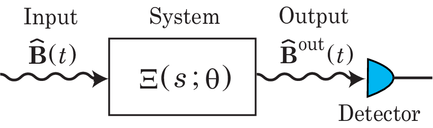
Refer to caption — Fig. 1: Setup of system identification for linear quantum systems. The experimenter can prepare a time-dependent input state, and perform a continuous-time measurement on the output, from which the unknown system parameters $\theta$ are estimated. The input-output relation is encoded in the transfer function $\Xi(s;\theta)$ .

In contrast to the classical case, a systematic methodology for linear quantum system identification has not yet been developed. Our aim is to fill this gap by investigating the following questions. (1) Identifiability: which system parameters can be in principle identified? (2) Identification method: given sufficient input-output data, how can we actually reconstruct system parameters? (3) Statistics: how well can we estimate unknown parameters by preparing appropriate input states and performing measurements on the output? The key fact to solve these problems is that, for linear systems, the Laplace domain input and output fields are related by a simple linear transformation represented by the transfer function matrix.

Below we give a more detailed account of the above-mentioned problems and the results obtained in this paper. First, the system identifiability is the property guaranteeing that all the system parameters can be in principle uniquely determined from the input-output data. This is actually an important notion in the classical case as well [37, 38, 39], and recently we find some proposals of those quantum analogues [40, 41] for nonlinear systems. In this paper, we show that minimal passive linear systems having the same transfer function (i.e. the equivalent class) are related by unitary transformations acting on the space of modes. Then, based on this result, we characterize a wide class of identifiable quantum linear networks, by employing the concept of infection introduced in [13, 15]. Next, the problem (2) boils down to that of identifying the transfer function, which can then be used to reconstruct the parameters of the system; in our case, those are the system’s (quadratic) Hamiltonian and its coupling to the environment, both described by appropriate matrices. In this paper, we provide two methods for finding the identifiable parameters and physical realizations for a given transfer function.

Beyond identifiability, it is important to investigate and compare the statistical performance of different estimation methods. By employing the well-established quantum estimation theory [42, 43], in particular the notion of quantum Fisher information, we investigate the problem of devising optimal (time dependent) coherent input states of a given energy, and output measurements. More precisely, we study the special case of a single-mode, single-input single-output (SISO) system in several scenarios with one or two unknown parameters. Moreover, for the single-mode SISO system, we show that the Heisenberg limit with respect to the input energy can be achieved for a non-classical input state. Note that, although this enhanced statistical performance could be expected from the quantum metrology theory [44], the important new concept is that this is the metrology for a dynamical system, where the static phase is now replaced by a dynamical phase represented by the transfer function. In fact this setup poses some new problems; for instance we need to optimize the frequency of the input field, which is not considered in the standard quantum metrology dealing with only static parameter estimation problems. These new problems can be formulated and solved thanks to the unitarity of the transfer function of linear passive systems, which is one of the reasons why we are chosen to investigate this class of systems separately from more general, active linear systems.

For reader’s convenience we summarize in advance the new concepts appearing in the quantum system identification problems studied in this paper, which are not found in the conventional identification theory for classical systems. The system’s input-output relation is represented by a transfer function having a special structure, which stems from the joint unitary evolution of the system and the field, and the fact that the interaction is passive. As consequence, the equivalence classes of parameters with the same output can be characterized in terms of unitary, rather than a general invertible matrices as is the case for classical systems. Note that limiting to a special class of linear systems does not mean straightforward applicability of the general identification theory for classical systems, but we need to take into account the essential feature of the focused system. Another specifically quantum aspect of the present theory is that all our results apply also to non-classical input states such as a single photon field; indeed, the transfer function can be used to describe the input-output relation even in such strong quantum scenarios [45], which is one of the advantages of the linear setup. This fact is important for the following two reasons. First, as mentioned in the above paragraph, the enhanced quantum system identification is achieved for non-classical input states. Second, such a passive linear systems driven by single photons behave essentially in the same way as some nonlinear/finite-level systems such as a dissipative qubit network driven by a single photon [46]; hence the theory developed in this paper is applicable to those genuine quantum systems beyond linear regime.

The paper is structured as follows. In Section II we introduce the setup of passive linear quantum systems, illustrated with realistic examples of system identification problems. In Section III, we give a necessary and sufficient condition for the identifiability of a passive linear system, which is then applied to several examples. Section IV describes the class of infective networks, which are shown to be completely identifiable. Section V provides two concrete identification methods. Section VI is devoted to the statistical analysis of the identification problem, using a Fisher information approach for the optimization over input states and output measurements. In Section VII, we briefly discuss the case of general (i.e. active) systems, pointing out some similarities and differences from the passive case, and formulate a conjecture regarding the structure of the equivalence classes.

Throughout the paper we will use the following notations: for a matrix $A=(a_{ij})$ , the symbols $A^{\dagger}$ and $A^{T}$ represent its Hermitian conjugate and transpose of $A$ , i.e., $A^{\dagger}=(a_{ji}^{*})$ and $A^{T}=(a_{ji})$ , respectively. For a matrix of operators, $\hat{A}=(\hat{a}_{ij})$ , we use the same notation, in which case $\hat{a}_{ij}^{*}$ denotes the adjoint to $\hat{a}_{ij}$ . $I_{n}$ denotes the $n\times n$ identity matrix.

A preliminary version of this paper was presented at the 52nd IEEE CDC [47].

II Passive linear quantum systems

In this section we briefly review the framework of linear classical and quantum dynamical systems, with several examples showing the need of system identification.

II-A Classical linear systems

A classical linear system is described by the set of differential equations

d\mbox{\boldmath$x$}(t)=A\mbox{\boldmath$x$}(t)dt+B\mbox{\boldmath$u$}(t)dt,~~~d\mbox{\boldmath$y$}(t)=C\mbox{\boldmath$x$}(t)dt+D\mbox{\boldmath$u$}(t)dt,

where $\mbox{\boldmath$x$}(t)\in\mathbb{R}^{n}$ is the state of the system, $\mbox{\boldmath$u$}(t)\in\mathbb{R}^{m}$ is an input signal, and $\mbox{\boldmath$y$}(t)\in\mathbb{R}^{k}$ is the output signal. The observer can control the input signal and observe the output, but does not have access to the internal state of the system. The input signal can be deterministic, in which case we deal with a set of ODEs, or stochastic, in which case the equations should be interpreted as SDEs. Apart from the input and the initial state of the system, the dynamics is determined by the (real) matrices $A,B,C,D$ .

To find the relation between input and output it is convenient to work in the Laplace domain. The Laplace transform of $\mbox{\boldmath$x$}(t)$ is defined by

{\cal L}[\mbox{\boldmath$x$}](s):=\int_{0}^{\infty}e^{-st}\mbox{\boldmath$x$}(t)dt,

(1)

where ${\rm Re}(s)>0$ . Then, we have the explicit input-output relation ${\cal L}[\mbox{\boldmath$y$}](s)=\Xi(s){\cal L}[\mbox{\boldmath$u$}](s)$ , where

\Xi(s)=C(sI-A)^{-1}B+D

(2)

is the transfer function matrix. System identification deals with the problem of estimating the matrices $A,B,C,D$ or certain parameters on which they depend, from the knowledge of the input and output processes. From (2) it is clear that the observer can at most determine the transfer function $\Xi(s)$ by preparing appropriate inputs and observing the output.

The identifiability problem is closely related to the fundamental system theory concepts of controllability and observability. The system is controllable if for any states $\mbox{\boldmath$x$}_{0},\mbox{\boldmath$x$}_{1}$ and times $t_{0}<t_{1}$ there exists a (piece-wise continuous) input $\mbox{\boldmath$u$}(t)$ such that the initial and final states are given by $\mbox{\boldmath$x$}(t_{0})=\mbox{\boldmath$x$}_{0}$ and $\mbox{\boldmath$x$}(t_{1})=\mbox{\boldmath$x$}_{1}$ , respectively. This is equivalent to the fact that the controllability matrix ${\cal C}=[B,AB,\ldots,A^{n-1}B]$ has full row rank. The system is observable if for any times $t_{0}<t_{1}$ , the initial state $\mbox{\boldmath$x$}(t_{0})=\mbox{\boldmath$x$}_{0}$ can be determined from the history of the input and output on the time interval $[t_{0},t_{1}]$ . This is in turn equivalent to the fact that the observability matrix ${\cal O}=[C^{T},(CA)^{T},\ldots,(CA^{n-1})^{T}]^{T}$ has full column rank.

The importance of these concepts for identifiability stems from the fact that if the system is not controllable or observable then there exists a lower dimensional system with the same transfer function as the original one. The former can be obtained from the latter by separating its coordinates via a canonical procedure called the Kalman decomposition. Therefore, in system identification it is natural to restrict the attention to minimal systems, i.e. systems which are both controllable and observable. As noted above, by appropriately choosing the input signal $\mbox{\boldmath$u$}(t)$ , the observer can effectively identify the transfer function $\Xi(s)$ , while other independent parameters in the system matrices are not identifiable in the absence of any prior knowledge. The following theorem gives a precise characterization of systems which are equivalent in the sense that they cannot be distinguished based on the input-output history [7].

Theorem II.1

Two minimal systems $(A,B,C,D)$ and $(A^{\prime},B^{\prime},C^{\prime},D^{\prime})$ have the same transfer function $\Xi(s)$ if and only if they are related by a similarity transformation, i.e. there exists an invertible $n\times n$ matrix $T$ such that

A^{\prime}=TAT^{-1},\quad B^{\prime}=TB,\quad C^{\prime}=CT^{-1},\quad D^{\prime}=D.

II-B Passive linear quantum system

A general linear quantum system with $n$ continuous variables modes is described by the column vectors of creation operators $\hat{\mbox{\boldmath$a$}}^{*}:=[\hat{a}^{*}_{1},\ldots,\hat{a}^{*}_{n}]^{T}$ and annihilation operators $\hat{\mbox{\boldmath$a$}}:=[\hat{a}_{1},\ldots,\hat{a}_{n}]^{T}$ satisfying the commutation relations

\hat{a}_{i}\hat{a}^{*}_{j}-\hat{a}^{*}_{j}\hat{a}_{i}=[\hat{a}_{i},\hat{a}^{*}_{j}]=\delta_{ij}\hat{1}.

(3)

The system has a quadratic Hamiltonian of the form

\hat{H}=\hat{\mbox{\boldmath$a$}}^{\dagger}\Omega\hat{\mbox{\boldmath$a$}}=[\hat{a}^{*}_{1},\ldots,\hat{a}^{*}_{n}]\left[\begin{array}[]{ccc}\Omega_{11}&\ldots&\Omega_{1n}\\ \vdots&&\vdots\\ \Omega_{n1}&\ldots&\Omega_{nn}\\ \end{array}\right]\left[\begin{array}[]{c}\hat{a}_{1}\\ \vdots\\ \hat{a}_{n}\\ \end{array}\right]

with $\Omega$ an $n\times n$ complex Hermitian matrix, and is coupled to $m$ bosonic quantum fields $\hat{\bf B}(t)=[\hat{B}_{1}(t),\dots,\hat{B}_{m}(t)]^{T}$ whose algebraic properties are characterized by the commutation relations

[\hat{B}_{i}(t),\hat{B}_{j}^{*}(s)]=\min\{s,t\}\delta_{ij}\hat{1},

or alternatively by

[\hat{b}_{i}(t),\hat{b}_{j}^{*}(s)]=\delta(t-s)\delta_{ij}\hat{1}.

(4)

where $\hat{\mbox{\boldmath$b$}}(t)=[\hat{b}_{1}(t),\ldots,\hat{b}_{m}(t)]^{T}$ is the white noise operator formally defined as $\hat{\mbox{\boldmath$b$}}(t)=d\hat{\bf B}(t)/dt$ .

The coupling between system and field is described by the following set of operators:

\hat{{\bf L}}=C\hat{\mbox{\boldmath$a$}}=\left[\begin{array}[]{ccc}c_{11}&\ldots&c_{1n}\\ \vdots&&\vdots\\ c_{m1}&\ldots&c_{mn}\\ \end{array}\right]\left[\begin{array}[]{c}\hat{a}_{1}\\ \vdots\\ \hat{a}_{n}\\ \end{array}\right],

with $c_{ij}$ a complex number. More precisely, the joint system-field evolution up to time $t$ is given by the unitary operator $\hat{U}(t)$ satisfying the quantum stochastic differential equation (QSDE) [48]

d\hat{U}(t)=\left(d\hat{\bf B}^{\dagger}(t)\hat{\bf L}-\hat{\bf L}^{\dagger}d\hat{\bf B}(t)+\frac{1}{2}\hat{\mbox{\boldmath$a$}}^{\dagger}A\hat{\mbox{\boldmath$a$}}dt\right)\hat{U}(t),

where

A:=-i\Omega-\frac{1}{2}C^{\dagger}C.

(5)

This type of system is called “passive”, because the operators do not involve the creation process such as $\hat{a}^{*}_{i}\hat{a}^{*}_{j}$ in $\hat{H}$ and $\hat{a}^{*}_{i}$ in $\hat{\bf L}$ , representing a purely dissipative evolution.

The Heisenberg evolution of the system operators is $\hat{\mbox{\boldmath$a$}}(t)=\hat{U}(t)^{*}\hat{\mbox{\boldmath$a$}}\hat{U}(t)$ , which by differentiation gives the equation

d\hat{\mbox{\boldmath$a$}}(t)=A\hat{\mbox{\boldmath$a$}}(t)dt-C^{\dagger}d\hat{\bf B}(t).

(6)

Similarly, the output process $\hat{\bf B}^{\rm out}(t)=\hat{U}(t)^{*}\hat{\bf B}(t)\hat{U}(t)$ satisfies the differential equation

d\hat{\bf B}^{\rm out}(t)=C\hat{\mbox{\boldmath$a$}}(t)dt+d\hat{\bf B}(t).

(7)

The Laplace transforms of $\hat{\mbox{\boldmath$a$}}(t)$ , $\hat{\mbox{\boldmath$b$}}(t)=d\hat{\bf B}(t)/dt$ , and $\hat{\mbox{\boldmath$b$}}^{\rm out}(t)=d\hat{\bf B}^{\rm out}(t)/dt$ are defined as in (1), for ${\rm Re}(s)>0$ . As we will be assuming that the system is stable, the initial state of the system is irrelevant in the long time limit, and we can set its mean to zero $\langle{\hat{\mbox{\boldmath$a$}}(0)}\rangle=0$ . In the Laplace domain the input-output relation is a simple multiplication

{\cal L}[\hat{\mbox{\boldmath$b$}}^{\rm out}](s)=\Xi(s){\cal L}[\hat{\mbox{\boldmath$b$}}](s),

(8)

where $\Xi(s)$ is the transfer function matrix:

\Xi(s):=I_{m}-C(sI-A)^{-1}C^{\dagger}.

(9)

With $s=-i\omega$ we define the frequency domain operators

\hat{\mbox{\boldmath$b$}}(\omega):=\mathcal{L}[\hat{\mbox{\boldmath$b$}}](-i\omega)=\frac{1}{\sqrt{2\pi}}\int_{-\infty}^{\infty}e^{i\omega t}\hat{\mbox{\boldmath$b$}}(t)

so that $\hat{\mbox{\boldmath$b$}}^{\rm out}(\omega)=\Xi(-i\omega)\hat{\mbox{\boldmath$b$}}(\omega)$ . Since $\hat{\mbox{\boldmath$b$}}^{\rm out}(\omega)$ must satisfy canonical commutation relations similar to (4), $\Xi(-i\omega)$ must be unitary for all $\omega$ [21].

II-C Examples of passive linear systems

Example II.1

The first example is an optical cavity illustrated in Fig. 2 (a). The intra-cavity field with mode $\hat{a}(t)$ couples to the incoming laser field $\hat{B}_{1}(t)$ and a vacuum $\hat{B}_{2}(t)$ ; then two outgoing fields $\hat{B}_{1}^{\rm out}(t)$ and $\hat{B}_{2}^{\rm out}(t)$ appear in the output ports. The system dynamics is given by

	$\displaystyle\hskip-20.00003ptd\hat{a}=(-i\omega_{o}-\kappa)\hat{a}dt-\sqrt{\kappa}d\hat{B}_{1}-\sqrt{\kappa}d\hat{B}_{2},$
	$\displaystyle\hskip-20.00003ptd\hat{B}_{1}^{\rm out}=\sqrt{\kappa}\hat{a}dt+d\hat{B}_{1},~~d\hat{B}_{2}^{\rm out}=\sqrt{\kappa}\hat{a}dt+d\hat{B}_{2},$		(10)

where $\kappa$ is the transmissivity of the coupling mirrors and $\omega_{o}$ is the detuning representing the frequency difference between the inner and outer optical fields. Note that $C^{\dagger}=[\sqrt{\kappa},\sqrt{\kappa}]$ and $\Omega=\omega_{o}$ . The role of this cavity system is low-pass filtering for the noisy incoming laser field $\hat{B}_{1}$ , and $\hat{B}_{2}^{\rm out}$ is the resultant mode-cleaned field which can be use for quantum information processing [49]. To effectively perform mode cleaning, we need to identify the parameter $\omega_{o}$ . In practice, the corresponding error signal can be detected by homodyne measuring the first output field $\hat{B}_{1}^{\rm out}$ , which is further used to lock the cavity path-length to attain $\omega_{o}=0$ by a piezo-actuator mounted on the mirror. Thanks to recent progress in nano-device engineering, it is possible to realize high-Q cavities, which can be used for storing optical light fields [50].

Example II.2

The next example is that of two large atomic ensembles trapped in a cavity (which will be adiabatically eliminated) having two input-output ports, as illustrated in Fig. 2 (b). The system variables of the $k$ th ensemble $(k=1,2)$ are the total angular momentum operators $(\hat{J}_{k}^{x},\hat{J}_{k}^{y},\hat{J}_{k}^{z})$ satisfying $[\hat{J}_{k}^{x},\hat{J}_{k}^{y}]=i\hat{J}_{k}^{z}\sim iJ$ ( $J\in{\mathbb{R}}$ ), where the approximation is taken due to the large ensemble limit; then, the “position” and “momentum” operators $\hat{q}_{k}=\hat{J}_{k}^{x}/\sqrt{J}$ , $\hat{p}_{k}=\hat{J}_{k}^{y}/\sqrt{J}$ serve as system variables. It was shown in [25, 27, 28] that a nontrivial coupling between the ensembles can be realized, which as a result leads to the following dynamical equation:

d\hat{\mbox{\boldmath$x$}}=-\frac{\kappa}{2}\left[\begin{array}[]{cc}Y&0\\ 0&Y\\ \end{array}\right]\hat{\mbox{\boldmath$x$}}dt+i\sqrt{\frac{\kappa}{2}}\left[\begin{array}[]{cc}-I_{2}&I_{2}\\ iY&iY\\ \end{array}\right]\left[\begin{array}[]{c}d\hat{\bf B}\\ d\hat{\bf B}^{*}\\ \end{array}\right],

where $\hat{\bf B}=[\hat{B}_{1},\hat{B}_{2}]^{T}$ , $\hat{\bf B}^{*}=[\hat{B}^{*}_{1},\hat{B}^{*}_{2}]^{T}$ ,

\hat{\mbox{\boldmath$x$}}=[\hat{q}_{1},\hat{q}_{2},\hat{p}_{1},\hat{p}_{2}]^{T},~~Y=\left[\begin{array}[]{cc}\cosh(2r)&-\sinh(2r)\\ -\sinh(2r)&\cosh(2r)\\ \end{array}\right].

and $\kappa$ and $r$ are system parameters. Since $Y>0$ , the system is stable and has a unique steady state; interestingly, it is the so-called pure two-mode squeezed state [3], whose covariance matrix is given by $V(\infty)={\rm diag}\{Y^{-1}/2,~Y/2\}$ . This implies that the two atomic ensembles are entangled. We emphasize the general fact that, if a linear system has a unique pure steady state, then it must be passive [29]. Actually, the vector of operators $\hat{\mbox{\boldmath$a$}}=[\hat{a}_{1},\hat{a}_{2}]^{T}$ defined by

\hat{\mbox{\boldmath$a$}}=\frac{1}{\sqrt{2}}[-iY^{1/2},~Y^{-1/2}]\hat{\mbox{\boldmath$x$}}

satisfies the CCR (3) and obeys

d\hat{\mbox{\boldmath$a$}}=-\frac{\kappa}{2}Y\hat{\mbox{\boldmath$a$}}dt-\sqrt{\kappa}Y^{1/2}d\hat{\bf B},~~d\hat{\bf B}^{\rm out}=\sqrt{\kappa}Y^{1/2}\hat{\mbox{\boldmath$a$}}dt+d\hat{\bf B}.

This is clearly a passive system with $\Omega=0$ and $C=\sqrt{\kappa}Y^{1/2}$ . (Note that the equation of $\hat{\mbox{\boldmath$x$}}$ can be uniquely recovered from that of $\hat{\mbox{\boldmath$a$}}$ .) Clearly, identifying the parameter $r$ is important, as it determines the amount of entanglement between the ensembles. The same fact holds for the more general case of pure Gaussian cluster states, which may be generated via a passive system composed of atomic ensembles [26], can be used for one-way quantum computing.

Example II.3

The last example is that of a medium of $N$ $\Lambda$ -type atoms trapped in a cavity [30], cf. Fig. 2 (c). Each atom has two metastable ground states $|{s}\rangle$ and $|{g}\rangle$ , and an excited state $|{e}\rangle$ . The e-g transition is naturally coupled to the cavity mode $\hat{a}_{1}$ with strength $g\sqrt{N}$ , whereas the s-e transition is induced by adding a classical magnetic field with time-varying Rabi frequency $\omega(t)$ . The system’s variables are the polarization operator $\hat{a}_{2}=\hat{\sigma}_{ge}/\sqrt{N}$ and the spin-wave operator $\hat{a}_{3}=\hat{\sigma}_{gs}/\sqrt{N}$ , where $\hat{\sigma}_{\bullet}$ is the collective lowering operator. As in the previous example, they can be well approximated by annihilation operators in the large ensemble limit, and as a result $\hat{\mbox{\boldmath$a$}}=[\hat{a}_{1},\hat{a}_{2},\hat{a}_{3}]^{T}$ obeys the following passive system;

	$\displaystyle\hskip-20.00003ptd\hat{\mbox{\boldmath$a$}}=\left[\begin{array}[]{ccc}-\kappa&ig\sqrt{N}&0\\ ig\sqrt{N}&-i\delta&i\omega\\ 0&i\omega^{*}&0\\ \end{array}\right]\hat{\mbox{\boldmath$a$}}dt-\left[\begin{array}[]{c}\sqrt{2\kappa}\\ 0\\ 0\\ \end{array}\right]d\hat{B},~~~$
	$\displaystyle\hskip-20.00003ptd\hat{B}^{\rm out}=\sqrt{2\kappa}\hat{a}_{1}dt+d\hat{B},$		(18)

where $\kappa$ denotes the cavity decay rate and $\delta$ is the detuning of the cavity center frequency and the s-e transition frequency. This system works as a quantum memory as follows. A state of the input optical field $\hat{B}(t)$ is transferred to that of the spin-wave mode $\hat{a}_{3}$ , and then it is preserved there by setting $\omega(t)=0$ . An effective pulse shaping method for $\omega(t)$ which achieves high fidelity state transfer and storage is presented in [30]. Such an optimal pulse depends on the system’s parameters, which therefore should be identified as accurately as possible. Note that several similar architectures for quantum memory have been proposed for instance in an inhomogeneously broadened ensemble of atoms or nitrogen-vacancy centers in diamond [31, 32, 33], nano-mechanical oscillators [34], or a general linear network [35], all of which are modeled by passive linear systems. We should emphasize that the passivity property is essential, as in general an active system violates the energy balance and does not realize a perfect state transfer.

III The system identifiability

This section begins with the problem formulation of system identification and the definition of identifiability. We then provide basic necessary and sufficient conditions for the passive linear system (6) and (7) to be identifiable. Some examples are given to illustrate the result.

III-A System identifiability

Broadly speaking, by system identification we mean the estimation of the parameters $\Omega$ and $C$ which completely characterize the linear quantum system (6) and (7). This task can be analyzed in various scenarios, depending on the experimenter’s ability to prepare the field’s input state and the system’s initial state, and the type of measurements used for extracting information about the dynamics. In the simplest experimental scenario the input field is prepared in a coherent state with a certain temporal shape

\langle{\hat{\mbox{\boldmath$b$}}(t)}\rangle=\beta(t),

and the experimenter can perform standard (e.g. homodyne and heterodyne) measurements on the output. We return to this scenario in section VI.

As noted before, in the frequency domain we have $\hat{\mbox{\boldmath$b$}}^{\rm out}(\omega)=\Xi(-i\omega)\hat{\mbox{\boldmath$b$}}(\omega)$ , so by taking expectation we get $\langle{\hat{\mbox{\boldmath$b$}}^{\rm out}}\rangle(\omega)=\Xi(-i\omega)\tilde{\beta}(\omega)$ , where $\tilde{\beta}(\omega)$ is the Fourier transform of $\beta(t)$ . Therefore, the experimenter can at most determine $\Xi(-i\omega)$ , and this can be done by preparing appropriate inputs (e.g. sinusoids with a certain frequency $\omega$ ), observing the outputs (e.g. by homodyne measurements) and computing their Fourier transforms.

In general, the system matrices may be modeled as depending on an unknown parameter vector $\theta\in\Theta$ such that

(\Omega,C)=(\Omega(\theta),C(\theta)),

(19)

and $\Xi(s)=\Xi(s;\theta)$ correspondingly. The task is then to estimate $\theta$ using the input and output relations (see Fig. 1). The identifiability of the system is defined as follows.

Definition III.1

The parameter $\theta$ is identifiable if $\Xi(s;\theta)=\Xi(s;\theta^{\prime})$ for all $s$ implies $\theta=\theta^{\prime}$ .

III-B Observability, controllability and minimality

The concepts of controllability and observability have a straightforward, though arguably non unique, extension to the quantum domain; see Section II-A for the classical case. The system defined by (6) and (7) is controllable if the following controllability matrix has full row rank:

{\cal C}=-[C^{\dagger},AC^{\dagger},\ldots,A^{n-1}C^{\dagger}].

(20)

Similarly, the system is observable if the observability matrix

{\cal O}=[C^{T},(CA)^{T},\ldots,(CA^{n-1})^{T}]^{T}

(21)

has full column rank. As in the classical case, if the system is not controllable or observable then there exists a lower dimensional system with the same transfer function as the original one. Thus, we focus on minimal, i.e. controllable and observable quantum systems. The following lemma shows that in the passive case we need to check only one of the controllability and observability conditions to verify that the system is minimal and stable.

Lemma III.1

For the quantum passive linear system (6) and (7), the controllability and the observability conditions are equivalent. Moreover, any minimal system is stable, i.e. $A$ is Hurwitz.

Proof:

From the result of systems theory [7], $(A,C^{\dagger})$ controllability is equivalent to the following condition: $yA=\lambda y,~\exists y,\lambda~\Rightarrow~yC^{\dagger}\neq 0$ . Then we have

zA^{\dagger}=\mu z,~\exists z,\mu~~\Rightarrow~~zC^{\dagger}\neq 0.

(22)

To prove (22), suppose that there exists a vector $z$ satisfying $zA^{\dagger}=\mu z$ and $zC^{\dagger}=0$ . This leads to $z\Omega=-i\mu z$ and $zC^{\dagger}C=0$ , yielding $zA=z(-i\Omega-C^{\dagger}C/2)=-\mu z$ . But together with $zC^{\dagger}=0$ , this is contradiction to the condition posed in the first line, thus (22) holds. Now again from the systems theory, (22) is the iff condition for $(A^{\dagger},C^{\dagger})$ controllability and it is equivalent to $(A,C)$ observability. The proof for the inverse direction is the same.

Let us move to prove the stability property. Because of the minimality, the system satisfies the condition (22); hence $z^{\dagger}$ is an eigenvector of $A$ and $\mu^{*}$ is the corresponding eigenvalue. Then the relation $zA^{\dagger}z^{\dagger}=\mu\|z^{\dagger}\|^{2}$ together with its complex conjugate lead to ${\rm Re}(\mu)=-\|Cz^{\dagger}\|^{2}/2\|z^{\dagger}\|^{2}$ , which is strictly negative due to $zC^{\dagger}\neq 0$ . Therefore $A$ is a Hurwitz matrix. ∎

III-C The identifiability conditions

As noted above, by appropriately choosing the input signal $\beta(t)$ , the observer can effectively identify the transfer function $\Xi(s)$ . The following theorem gives a precise characterization of systems which are equivalent in the sense that they cannot be distinguished based on only the input-output relation.

Theorem III.1

Let $(\Omega_{1},C_{1})$ and $(\Omega_{2},C_{2})$ be two passive linear systems as defined in (6) and (7), and assume that both systems are minimal. Then they have the same transfer function if and only if there exists a unitary matrix $U$ such that

\Omega_{2}=U\Omega_{1}U^{\dagger},~~~C_{2}=C_{1}U^{\dagger}.

(23)

Proof:

It is well known that two minimal systems have the same transfer functions

C_{1}(sI-A_{1})^{-1}C_{1}^{\dagger}=C_{2}(sI-A_{2})^{-1}C_{2}^{\dagger},

(we here omit the trivial constant term $I$ ) iff there exists an invertible matrix $U$ satisfying

A_{2}=UA_{1}U^{-1},~~C_{2}^{\dagger}=UC_{1}^{\dagger},~~C_{2}=C_{1}U^{-1}.

(24)

Note that $U$ is not assumed to be unitary. Using the second and third conditions we have $C_{1}(U^{\dagger}U)=C_{1}$ , which further gives $[U^{\dagger}U,~C_{1}^{\dagger}C_{1}]=0$ . Also, applying the second and third conditions to the first one, we have $\Omega_{2}=U\Omega_{1}U^{-1}$ . Then, because $\Omega_{i}$ is a Hermitian matrix, $[U^{\dagger}U,~\Omega_{1}]=0$ holds. Combining these two results we obtain $[U^{\dagger}U,~A_{1}]=0$ . Therefore we have

C_{1}A_{1}=C_{1}(U^{\dagger}U)A_{1}=C_{1}A_{1}(U^{\dagger}U),

which means that the observability matrix ${\cal O}$ satisfies ${\cal O}={\cal O}U^{\dagger}U$ . Because of the assumption that ${\cal O}$ is of full rank, $U$ is unitary. Therefore the conditions (24) are reduced to (23). ∎

For a parameterized model the identifiability condition is given by the following.

Corollary III.1

Let $(\Omega(\theta),C(\theta))$ be a minimal system with unknown parameter vector $\theta\in\Theta$ . Then $\theta$ is identifiable if and only if

\Omega(\theta^{\prime})=U\Omega(\theta)U^{\dagger},~~~C(\theta^{\prime})=C(\theta)U^{\dagger}

implies $\theta=\theta^{\prime}$ .

The above result can be interpreted as follows. The matrix $U$ corresponds to the coordinate transformation $\hat{\mbox{\boldmath$a$}}^{\prime}=U\hat{\mbox{\boldmath$a$}}$ and the unitarity of $U$ means that the canonical commutation relation (3) is preserved. Note that if the system variables contain classical components, $U$ would not necessarily be unitary. Similarly, if the system is not passive, then one needs to consider both $\hat{\mbox{\boldmath$a$}}$ and $\hat{\mbox{\boldmath$a$}}^{*}$ as coordinates, and corresponding doubled-up transfer matrices [51].

In addition to the above corollary, we give another criterion for testing the identifiability. Note this result does not require the minimality of the system.

Lemma III.2

The parameter $\theta$ is identifiable if and only if

C(\theta)\Omega(\theta)^{k}C(\theta)^{\dagger}=C(\theta^{\prime})\Omega(\theta^{\prime})^{k}C(\theta^{\prime})^{\dagger},~~~\forall k

(25)

implies $\theta=\theta^{\prime}$ .

Proof:

For simplicity let us denote $C:=C(\theta),C^{\prime}:=C(\theta^{\prime})$ and similarly for $\Omega$ and $A$ . By expanding the equation $\Xi(s;\theta)=\Xi(s;\theta^{\prime})$ with respect to $s$ and comparing their coefficients, we have $CA^{k}C^{\dagger}=C^{\prime}A^{\prime k}C^{\prime\dagger}$ for all $k$ , and thus

C\big(-i\Omega-\frac{1}{2}C^{\dagger}C\big)^{k}C^{\dagger}=C^{\prime}\big(-i\Omega^{\prime}-\frac{1}{2}C^{\prime\dagger}C^{\prime}\big)^{k}C^{\prime\dagger}.

This $k$ -th order polynomial is composed of the linear combination of $C[(C^{\dagger}C)^{p}\circ\Omega^{q}]C^{\dagger}$ with $p+q=k$ , where $\circ$ means the symmetrization, e.g. $(C^{\dagger}C)^{1}\circ\Omega^{2}=(C^{\dagger}C)\Omega^{2}+\Omega(C^{\dagger}C)\Omega+\Omega^{2}(C^{\dagger}C)^{2}$ for $k=3$ . Then (25) can be proven by induction with respect to $k$ . ∎

III-D Examples

We here apply the identifiability conditions to some systems. The critical assumption is that we have some a priori information about the system, such as the structure of the network and some parameters. This a priori knowledge helps us to reduce the size of the equivalence class of the system and in some cases even to exactly identify the system, as will be demonstrated.

Example III.1

We begin with the simple cavity system studied in Example II.1. In this case, $\Omega=\omega_{o}$ and $C^{\dagger}=[\sqrt{\kappa},\sqrt{\kappa}]^{T}$ , where we assume that $\kappa$ is a known parameter. Now, from Theorem III.1, the equivalence class is generated by a trivial $1\times 1$ unitary matrix $U=e^{i\phi}$ ; but clearly $C=CU^{\dagger}$ imposes $U=1$ , hence from Corollary III.1 $\omega_{o}$ is identifiable.

Example III.2

Next let us consider the system in Example II.2, where $\Omega=0$ and $C=\sqrt{\kappa}Y^{1/2}$ . It is easy to see that the system is minimal. Then Theorem III.1 states that the equivalence class is generated by a unitary matrix $U$ as

\Omega^{\prime}=0,~~~C^{\prime}=CU^{\dagger}=\sqrt{\kappa}\left[\begin{array}[]{cc}\cosh(r)&-\sinh(r)\\ -\sinh(r)&\cosh(r)\\ \end{array}\right]U^{\dagger}.

Now, we know that $C^{\prime}$ is positive symmetric and the (1,1) and (2,2) elements are the same; this a priori knowledge allows only $U=I_{2}$ , so the parameters are identifiable.

Example III.3

The memory system shown in Example II.3 is a passive system essentially with

C=[\sqrt{2\kappa},~0,~0],~~\Omega(\theta)=\left[\begin{array}[]{ccc}0&\theta_{1}&0\\ \theta_{1}&0&\theta_{2}\\ 0&\theta_{2}&0\\ \end{array}\right],

(26)

where $(\theta_{1},\theta_{2})$ are unknown coupling constants to be identified (we assume $\delta=0$ ).

We immediately see that the system is controllable and accordingly minimal. Thus, we can apply Theorem III.1, showing that the equivalence class of the system is generated by the unitary matrix $U$ . But since we know the structure of the matrices $\Omega$ and $C$ , it follows that $U$ must be either $U_{1}={\rm Diag}(1,1,1)$ , $U_{2}={\rm Diag}(1,-1,1)$ , $U_{3}={\rm Diag}(1,1,-1)$ , or $U_{4}={\rm Diag}(1,-1,-1)$ . This means that the systems with parameter $\theta=(\theta_{1},\theta_{2})$ , $(-\theta_{1},\theta_{2}),(\theta_{1},-\theta_{2})$ , and $(-\theta_{1},-\theta_{2})$ have the same transfer function. Therefore the parameters $\theta_{1}$ and $\theta_{2}$ are identifiable up to the sign, i.e. $\theta$ is locally identifiable but not globally [38].

An alternative proof of the above result is obtained by using Lemma III.2. Actually we compute

	$\displaystyle\hskip-10.00002ptC\Omega(\theta)C^{\dagger}=0,~~~C\Omega(\theta)^{2}C^{\dagger}=2\kappa\theta_{1}^{2},$
	$\displaystyle\hskip-10.00002ptC\Omega(\theta)^{3}C^{\dagger}=0,~~~C\Omega(\theta)^{4}C^{\dagger}=2\kappa\theta_{1}^{2}(\theta_{1}^{2}+\theta_{2}^{2})$

yielding $\theta_{1}^{2}=\theta_{1}^{\prime 2}$ and $\theta_{2}^{2}=\theta_{2}^{\prime 2}$ hold, if $\theta_{1}\neq 0$ . Thus we have the same conclusion as above.

A third route is to look directly at the transfer function:

\Xi(s)=\frac{s^{3}-\kappa s^{2}+(\theta_{1}^{2}+\theta_{2}^{2})s-\kappa\theta_{2}^{2}}{s^{3}+\kappa s^{2}+(\theta_{1}^{2}+\theta_{2}^{2})s+\kappa\theta_{2}^{2}},

and note that the poles give us enough information to determine both $\theta_{1}^{2}$ and $\theta_{2}^{2}$ . Note when $\theta_{1}=0$ (i.e., there is no connection between $\hat{a}_{1}$ and $\hat{a}_{2}$ ), $\Xi(s)=(s-\kappa)/(s+\kappa)$ , showing that the system is clearly not minimal; actually in this case $\theta_{2}$ cannot be estimated.

Example III.4

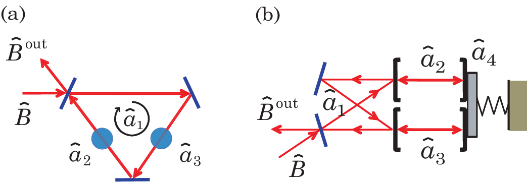
Let us consider the large atomic ensemble network depicted in Fig. 3 (a). The cavity field $\hat{a}_{1}$ is coupled to the input field and is connected to the ensembles with modes $\hat{a}_{2}$ and $\hat{a}_{3}$ which correspond to the collective lowering operators of the ensembles [25]. The system Hamiltonian is given by $\hat{H}=\Delta\hat{a}_{2}^{*}\hat{a}_{2}+\theta_{1}(\hat{a}_{1}^{*}\hat{a}_{2}+\hat{a}_{1}\hat{a}_{2}^{*})+\theta_{2}(\hat{a}_{1}^{*}\hat{a}_{3}+\hat{a}_{1}\hat{a}_{3}^{*})$ , hence we have

\Omega(\theta)=\left[\begin{array}[]{ccc}0&\theta_{1}&\theta_{2}\\ \theta_{1}&\Delta&0\\ \theta_{2}&0&0\\ \end{array}\right].

The $C$ matrix is the same as in (26).

The additional detuning Hamiltonian $\Delta\hat{a}_{2}^{*}\hat{a}_{2}$ is necessary for the parameters $\theta_{1}$ and $\theta_{2}$ to be identifiable, because the system is minimal only when $\Delta\neq 0$ . In fact, when $\Delta=0$ we cannot distinguish the two ensembles, thus the system is not identifiable. So we assume $\Delta\neq 0$ and apply Theorem III.1. The constraint $C=CU^{\dagger}$ implies that $U$ must be of the form $U={\rm Diag}(1,\tilde{U})$ with $\tilde{U}$ a $2\times 2$ unitary matrix. Then the equivalence class is characterized by

\Omega^{\prime}=\left[\begin{array}[]{cc}1&0^{T}\\ 0&\tilde{U}\\ \end{array}\right]\left[\begin{array}[]{cc}0&\theta^{T}\\ \theta&\Lambda\\ \end{array}\right]\left[\begin{array}[]{cc}1&0^{T}\\ 0&\tilde{U}^{\dagger}\\ \end{array}\right]=\left[\begin{array}[]{cc}0&(\tilde{U}\theta)^{\dagger}\\ \tilde{U}\theta&\tilde{U}\Lambda\tilde{U}^{\dagger}\\ \end{array}\right],

where $\theta=[\theta_{1},\theta_{2}]^{T}$ and $\Lambda={\rm Diag}(\Delta,0)$ . Now we know that the matrix $\Omega^{\prime}$ is of the same form as $\Omega$ , which yields additional constraint on $\tilde{U}$ , i.e. $\tilde{U}\Lambda\tilde{U}^{\dagger}=\Lambda$ , or equivalently $[\tilde{U},\Lambda]=0$ . This readily clarifies that $\tilde{U}$ is diagonal; hence together with $\tilde{U}\theta\in{\mathbb{R}}^{2}$ , we conclude that the parameters $\theta_{1}$ and $\theta_{2}$ are identifiable up to the sign.

Example III.5

The last example is a linear network composed of cavities and an opto-mechanical oscillator shown in Fig. 3 (b). This specific configuration is inspired by [52] and the oscillator can serve as a quantum memory. The oscillator with phonon mode $\hat{a}_{4}$ couples to two cavities with modes $(\hat{a}_{2},\hat{a}_{3})$ , through radiation pressure force; particularly with the dissipative (red-sideband) regime the coupling Hamiltonian takes a passive form [53]. The two cavities further interact with a bow-tie type cavity with mode $\hat{a}_{1}$ . As a result, the system Hamiltonian is given by

	$\displaystyle\hskip-10.00002pt\hat{H}=\theta_{1}(\hat{a}_{1}^{}\hat{a}_{2}+\hat{a}_{1}\hat{a}_{2}^{})+\theta_{2}(\hat{a}_{1}^{}\hat{a}_{3}+\hat{a}_{1}\hat{a}_{3}^{})$
	$\displaystyle\hskip 10.00002pt\mbox{}+\theta_{3}(\hat{a}_{2}^{}\hat{a}_{4}+\hat{a}_{2}\hat{a}_{4}^{})+\theta_{4}(\hat{a}_{3}^{}\hat{a}_{4}+\hat{a}_{3}\hat{a}_{4}^{}),$

thus we have

\Omega(\theta)=\left[\begin{array}[]{cccc}0&\theta_{1}&\theta_{2}&0\\ \theta_{1}&0&0&\theta_{3}\\ \theta_{2}&0&0&\theta_{4}\\ 0&\theta_{3}&\theta_{4}&0\\ \end{array}\right],

while the $C$ matrix is given by $C=[\sqrt{2\kappa},~0,~0,~0]$ .

Let us first check the minimality. A direct computation shows that the observability matrix ${\cal O}$ satisfies ${\rm det}({\cal O})=4\kappa^{2}(\theta_{1}\theta_{3}+\theta_{2}\theta_{4})^{2}(\theta_{2}\theta_{3}-\theta_{1}\theta_{4})$ . Hence, we consider the minimal system satisfying ${\rm det}({\cal O})\neq 0$ . Then from Theorem III.1, the equivalence class is generated in terms of the unitary $U={\rm Diag}(1,\tilde{U})$ with $\tilde{U}$ a $3\times 3$ unitary matrix, and it is parameterized by

\Omega^{\prime}=\left[\begin{array}[]{cc}0&[\theta_{12}^{T}~~0]\tilde{U}^{\dagger}\\ \tilde{U}\left[\begin{array}[]{c}\theta_{12}\\ 0\\ \end{array}\right]&\tilde{U}\Theta\tilde{U}^{\dagger}\\ \end{array}\right],~~\Theta=\left[\begin{array}[]{cc}0&\theta_{34}\\ \theta_{34}^{T}&0\\ \end{array}\right],

where $\theta_{12}=[\theta_{1},\theta_{2}]^{T}$ , $\theta_{34}=[\theta_{3},\theta_{4}]^{T}$ . The structure of the matrix $\Omega^{\prime}$ further imposes the additional constraint on $\tilde{U}$ , which as a result yields $\tilde{U}={\rm Diag}(V,1)$ with $V$ a $2\times 2$ orthogonal matrix. Therefore, the equivalence class is the system whose Hamiltonian matrix is characterized by

\Omega^{\prime}=\left[\begin{array}[]{ccc}0&\theta_{12}^{T}V^{T}&0\\ V\theta_{12}&O&V\theta_{34}\\ 0&\theta_{34}^{T}V^{T}&0\\ \end{array}\right].

Hence, from Theorem III.1, the systems specified by $(\Omega^{\prime},C)$ have the same transfer function for all $V$ . Thus, this system is not (completely) identifiable. However, if for instance the second cavity mode $\hat{a}_{2}$ is detuned and as consequence the (2,2) element of $\Omega$ is nonzero, then the system gains the identifiability property.

IV Network identification; the infection condition

As demonstrated in Section III, in order to establish the identifiability of a given system, we need to carry out certain model specific calculations ruling out the existence of non-trivial unitaries in Theorem 3.1. It would therefore be useful to find an identifiability criterion which applies to a general class of systems. In this section we describe such a criterion which relies on the special topological structure of the Hamiltonian. Similar results have been found in different contexts [13, 15].

Let $\mathcal{V}$ be the set of vertices representing the modes of our continuous variables system. The interactions between the different modes are modeled by the set of edges $\mathcal{E}$ over $\mathcal{V}$ : $\mathcal{E}\subset\mathcal{V}\times\mathcal{V}$ , so that two modes $i$ and $j$ interact if they are connected by an edge. More precisely, we assume that the matrix $\Omega$ describing the system Hamiltonian is of the form

\Omega(\theta)=\sum_{(i,j)\in\mathcal{E}}\omega_{i,j}(\theta)(e_{i}e_{j}^{T}+e_{j}e_{i}^{T}),

(27)

where $\omega_{i,j}(\theta)$ are unknown real coefficients which make up the parameter $\theta$ and $e_{i}=[0,\cdots,1,\cdots,0]^{T}$ is the basis vector having zeros except the $i$ th element. We further assume that the coupling between the system and the field is known and specified by the matrix $C$ whose support is spanned by a set of basis vectors $\{e_{i}:i\in\mathcal{I}\}$ for some set of vertices $\mathcal{I}$ , the restriction of $C^{\dagger}C$ to this subspace being strictly positive.

The crucial property we will require of $\mathcal{I}$ is that it is infecting for the graph $(\mathcal{V},\mathcal{E})$ , which can be defined sequentially by the following conditions (see Fig. 4):

(i)

At the beginning the vertices in $\mathcal{I}$ are infected;
(ii)

If an infected vertex has only one non-infected neighbor, the neighbor gets infected;
(iii)

After some interactions all nodes end up infected.

Roughly speaking, this infection property means that the network is similar to a “chain”, where the neighboring nodes are coupled to each other. Such a chain structure often appears in practical situations, and as shown in [54], it can be fully controlled by only accessing to its local subsystem. Also it is notable that in general a chain structure realizes fast spread of quantum information [55] and is thus suitable for e.g. distributing quantum entanglement. The result we present here is that such a useful network is always identifiable.

Lemma IV.1

Let $\Omega(\theta)$ be given by (27), and assume that the support of $C$ is spanned by $\{e_{i}:i\in\mathcal{I}\}$ with $(\mathcal{I},\mathcal{V},\mathcal{E})$ having the infecting property. Then, the system is minimal.

Proof:

From the assumption, at least one vertex $i_{0}\in\mathcal{I}$ is connected to exactly one vertex $j_{0}\in\mathcal{I}^{c}$ . Thus, $\Omega(\theta)$ can be written as

$\displaystyle\Omega(\theta)$	$\displaystyle=$	$\displaystyle\omega_{i_{0},j_{0}}(\theta)(e_{i_{0}}e_{j_{0}}^{T}+e_{j_{0}}e_{i_{0}}^{T})$
	$\displaystyle+$	$\displaystyle\sum_{i\in\mathcal{I},i\neq i_{0}}\sum_{j\in\mathcal{I}^{c}}\omega_{i,j}(\theta)(e_{i}e_{j}^{T}+e_{j}e_{i}^{T})$
	$\displaystyle+$	$\displaystyle\sum_{i,j\in\mathcal{I}}\omega_{i,j}(\theta)(e_{i}e_{j}^{T}+e_{j}e_{i}^{T})$
	$\displaystyle+$	$\displaystyle\sum_{i,j\in\mathcal{I}^{c}}\omega_{i,j}(\theta)(e_{i}e_{j}^{T}+e_{j}e_{i}^{T}).$

This readily leads to

\Omega(\theta)e_{i_{0}}=\omega_{i_{0},j_{0}}(\theta)e_{j_{0}}+2\sum_{j\in\mathcal{I}}\omega_{i_{0},j}(\theta)e_{j}.

Also clearly $C^{\dagger}Ce_{i_{0}}$ is spanned by the vectors $\{e_{i}:i\in{\cal I}\}$ . These two facts imply that $Ae_{i_{0}}=(-i\Omega-C^{\dagger}C/2)e_{i_{0}}$ is spanned by $e_{j_{0}}$ and $\{e_{i}:i\in{\cal I}\}$ . In other words, $C^{\dagger}$ and $Ae_{i_{0}}$ generate a new infecting set ${\cal I}^{\prime}={\cal I}\cup\{j_{0}\}$ . Repeating this procedure, we find that the controllability matrix (20), ${\cal C}=-[C^{\dagger},AC^{\dagger},\ldots,A^{n-1}C^{\dagger}]$ , is of full rank, thus the system is controllable. This further implies from Lemma III.1 that the system is observable, thus as a result it is minimal. ∎

Theorem IV.1

Proof:

First, from Lemma IV.1 we can apply Theorem III.1; the two parameters are in the same equivalence class if and only if there exists an $n\times n$ unitary matrix $U$ such that

\Omega(\theta_{2})=U\Omega(\theta_{1})U^{\dagger},

(28)

and $C=CU$ . The latter condition implies $[U,C^{\dagger}C]=0$ and in particular $U$ commutes with projection $P$ onto the support of $C^{\dagger}C$ so that

U=\left[\begin{array}[]{c|c}I&0\\ \hline\cr 0&V\\ \end{array}\right]

(29)

with $V$ unitary on the orthogonal complement of the support of $C$ . Let us write the Hamiltonian in the block form according to the partition $\mathcal{J}=\mathcal{I}\cup\mathcal{I}^{c}$ :

\Omega(\theta)=\left[\begin{array}[]{c|c}\Omega_{11}(\theta)&\Omega_{12}(\theta)\\ \hline\cr\Omega_{21}(\theta)&\Omega_{22}(\theta)\\ \end{array}\right].

Then (28) implies that

$\displaystyle\Omega_{11}(\theta_{2})$	$\displaystyle=$	$\displaystyle\Omega_{11}(\theta_{1}),$
$\displaystyle\Omega_{12}(\theta_{2})$	$\displaystyle=$	$\displaystyle\Omega_{12}(\theta_{1})V^{\dagger},$
$\displaystyle\Omega_{22}(\theta_{2})$	$\displaystyle=$	$\displaystyle V\Omega_{22}(\theta_{1})V^{\dagger}.$	(30)

The first equation of (30) means that

\omega_{i,j}(\theta_{1})=\omega_{i,j}(\theta_{2}),\qquad i,j\in\mathcal{I}.

(31)

Furthermore, since $\mathcal{I}$ is infecting, there exists at least one vertex $i_{0}\in\mathcal{I}$ which is connected to exactly one vertex $j_{0}\in\mathcal{I}^{c}$ , so that the off-diagonal block $\Omega_{12}(\theta)$ can be written as

	$\displaystyle\left[\begin{array}[]{c\|c}0&\Omega_{12}(\theta)\\ \hline\cr 0&0\\ \end{array}\right]$	$\displaystyle=$	$\displaystyle\omega_{i_{0},j_{0}}(\theta)(e_{i_{0}}e_{j_{0}}^{T}+e_{j_{0}}e_{i_{0}}^{T})$
		$\displaystyle+$	$\displaystyle\sum_{i\in\mathcal{I},i\neq i_{0}}\sum_{j\in\mathcal{I}^{c}}\omega_{i,j}(\theta)(e_{i}e_{j}^{T}+e_{j}e_{i}^{T}).$

The second equation of (30) then implies

\omega_{i_{0},j_{0}}(\theta_{1})Ue_{j_{0}}=\omega_{i_{0},j_{0}}(\theta_{2})e_{j_{0}},

which means that $e_{j_{0}}$ is an eigenvector of $U$ and $\omega_{i_{0},j_{0}}(\theta_{2})=\exp(i\phi_{0})\omega_{i_{0},j_{0}}(\theta_{1})$ for some phase $\phi_{0}$ . But since the coefficients of $\Omega(\theta)$ are assumed to be real, this implies that

\omega_{i_{0},j_{0}}(\theta_{1})=\omega_{i_{0},j_{0}}(\theta_{2}),\qquad i_{0}\in\mathcal{I},~~j_{0}\in\mathcal{I}^{c}.

(33)

Additionally, since $Ue_{j_{0}}=e_{j_{0}}$ , a decomposition of the form (29) holds with the identity block supported by the index set $\mathcal{I}^{\prime}=\mathcal{I}\cup\{j_{0}\}$ .

The same argument can now be repeated for the set $\mathcal{I}^{\prime}$ , and by using the infecting property, all vertices will be eventually included in the growing set of indices, so that at the end we have $\Omega(\theta_{1})=\Omega(\theta_{2})$ . Consequently, from Corollary III.1, the system is identifiable. ∎

From this result, we now readily see that the system in Example 3.3 in Section III-D is identifiable, since clearly this system has a chain-type structure and is thus infecting. On the other hand, the systems of Examples 3.4 and 3.5 have the tree and ring structures, respectively, which are thus not infecting. Hence, Theorem IV.1 states nothing about the identifiability of these systems; in fact, as shown there, the tree system is identifiable, while the ring one is not.

V Methods for system matrices identification

Let us consider the situation where we have constructed the transfer function matrix $\Xi(s)$ , using the input-output data; this is indeed possible via several techniques [7]. In the SISO case, this means that we have determined the coefficients $(a_{i},c_{i})$ of the following rational function:

\Xi(s)=1+\frac{c_{n-1}s^{n-1}+\cdots+c_{0}}{s^{n}+a_{n-1}s^{n-1}+\cdots+a_{0}}.

Then the following set of system matrices

	$\displaystyle\hskip-10.00002ptA_{0}=\left[\begin{array}[]{cccc}0&1&&0\\ &\ddots&\ddots&\\ 0&&0&1\\ -a_{0}&-a_{1}&&-a_{n-1}\\ \end{array}\right],~~B_{0}=\left[\begin{array}[]{c}0\\ \vdots\\ 0\\ 1\\ \end{array}\right],~~$
	$\displaystyle\hskip-10.00002ptC_{0}=[c_{0},\cdots,c_{n-1}],$		(43)

constitute a realization of $\Xi(s)$ in the sense that $\Xi(s)=1+C_{0}(sI-A_{0})^{-1}B_{0}$ . Any other realization having the same transfer function can be generated via the similarity transformation

A=TA_{0}T^{-1},~~B=TB_{0},~~C=C_{0}T^{-1}.

(44)

However, the matrices (V) do not satisfy the constraints imposed on passive linear quantum systems. This means that, for general $T$ , the transformation (44) does not yield the set of coefficient matrices of a quantum system; e.g., the relation $B=-C^{\dagger}$ is not satisfied. Clearly, in this case, the system matrices $(\Omega,C)$ cannot be reconstructed. This is an important issue, since from the physics viewpoint we are often interested in the system matrices and the system parameters, rather than the transfer function. Therefore, we need to find a special class of $T$ so that the coefficient matrices (44) satisfy the constraints and that the system matrices can be reconstructed. In this section, we provide two concrete procedures to achieve this goal.

V-A Reconstruction of system matrices

Let $(A_{0},B_{0},C_{0})$ be constructed from the transfer function of a minimal quantum system (6) and (7) (note that now it is not limited to the SISO case). Then, for a certain matrix $T$ , the matrices (44) satisfy the constraints (5), which immediately yields $A+A^{\dagger}+C^{\dagger}C=0$ , and $B=-C^{\dagger}$ . These conditions are written in terms of $(A_{0},B_{0},C_{0})$ as

(T^{\dagger}T)A_{0}+A_{0}^{\dagger}(T^{\dagger}T)+C_{0}^{\dagger}C_{0}=0

(45)

and $(T^{\dagger}T)B_{0}=-C_{0}^{\dagger}$ . Now the system is assumed to be minimal, thus $A_{0}$ is Hurwitz from Lemma III.1. This means that the Lyapunov equation (45) has a unique solution $T^{\dagger}T>0$ . Accordingly, we have the diagonalization $T^{\dagger}T=U_{0}\Lambda U_{0}^{\dagger}$ , where $\Lambda>0$ is a diagonal matrix composed of eigenvalues of $T^{\dagger}T$ and $U_{0}$ the corresponding unitary matrix. Then, $T$ is fully characterized by an arbitrary unitary matrix $U$ as

T=U\sqrt{\Lambda}U_{0}^{\dagger},

(46)

where $\sqrt{\Lambda}$ is a positive diagonal matrix satisfying $(\sqrt{\Lambda})^{2}=\Lambda$ . This $T$ generates the equivalence class of quantum systems. In particular, by denoting $T_{0}=\sqrt{\Lambda}U_{0}^{\dagger}$ , we can interpret that $T$ first transforms the matrices $(A_{0},B_{0},C_{0})$ to those corresponding to the quantum system, $(T_{0}A_{0}T_{0}^{-1},T_{0}B_{0},C_{0}T_{0}^{-1})$ ; then we obtain the unitary equivalence class by acting a unitary matrix $U$ on those matrices. See Fig. 5.

Now the system matrices $(\Omega,C)$ can be reconstructed. It follows from (5) that $A-A^{\dagger}=-2i\Omega$ , which thus together with (44) and (46) yields

	$\displaystyle\hskip-30.00005pt\Omega=U\Omega_{0}U^{\dagger},~~~$
	$\displaystyle\hskip-30.00005pt\Omega_{0}=\frac{i}{2}\Big[\sqrt{\Lambda}U_{0}^{\dagger}A_{0}U_{0}\sqrt{\Lambda^{-1}}-\sqrt{\Lambda^{-1}}U_{0}^{\dagger}A_{0}^{\dagger}U_{0}\sqrt{\Lambda}\Big].$		(47)

Similarly, from $C=C_{0}T^{-1}$ we have

C=(C_{0}U_{0}\sqrt{\Lambda^{-1}})U^{\dagger}.

(48)

These are exactly of the form (23) in Theorem III.1. Hence, the following theorem holds. Note that a similar result is found in [56].

Theorem V.1

Let $A_{0}$ and $C_{0}$ be matrices directly obtained from the transfer function $\Xi(s)$ , e.g. (V) in the SISO case. Then, the equivalence class of system matrices $(\Omega,C)$ is given by (47) and (48) with unitary matrix $U$ , where $\Lambda$ and $U_{0}$ are constructed from the solution of (45).

V-B Example

Let us consider a two-mode SISO system with only single mode accessible and assume that the following transfer function has been experimentally obtained:

\Xi(s)=1+\frac{c_{1}s}{s^{2}+a_{1}s+a_{0}},

where $a_{0},a_{1}>0$ and $c_{1}$ are real numbers. (As we will explain later, $c_{1}=-2a_{1}$ is satisfied.) For this transfer function we take the typical realization (V); i.e.,

A_{0}=\left[\begin{array}[]{cc}0&1\\ -a_{0}&-a_{1}\\ \end{array}\right],~~B_{0}=\left[\begin{array}[]{c}0\\ 1\\ \end{array}\right],~~C_{0}=[0,~c_{1}].

Note that $B_{0}=-C_{0}^{\dagger}$ does not hold in general. With this choice, the Lyapunov equation (45) has the following unique solution:

T^{\dagger}T=\frac{c_{1}^{2}}{2a_{1}}\left[\begin{array}[]{cc}a_{0}&0\\ 0&1\\ \end{array}\right],

which is equal to $\Lambda$ , and now $U_{0}=I$ . Thus, the equivalence class of the system matrices are given by (47) and (48) with

\Omega_{0}=\left[\begin{array}[]{cc}0&i\sqrt{a_{0}}\\ -i\sqrt{a_{0}}&0\\ \end{array}\right],~~C_{0}U_{0}\sqrt{\Lambda^{-1}}=[0,-\sqrt{2a_{1}}].

In particular, when choosing $U=[0,~-1~;~i,~0]$ , we have

\Omega=\left[\begin{array}[]{cc}0&\sqrt{a_{0}}\\ \sqrt{a_{0}}&0\\ \end{array}\right],~~C=[\sqrt{2a_{1}},~0],

which have exactly the same forms as the system matrices in Example 3.3 with specifically $\theta_{2}=0$ taken. That is, the coupling strength between the system modes is identified as $\sqrt{a_{0}}$ , and the system-field coupling strength is identified as $\sqrt{2a_{1}}$ . Note that the condition $(T^{\dagger}T)B_{0}=-C_{0}^{\dagger}$ yields $c_{1}=-2a_{1}$ ; indeed this relation is satisfied for the two-mode system, as easily seen by again setting $\theta_{2}=0$ in Example 3.3.

V-C Direct reconstruction of system matrices from the transfer function

In Section V-A we have shown that the equivalent class of system matrices can be reconstructed through typical realization methods employed in classical system theory. We here present another procedure that directly reconstructs the equivalence class.

We begin with the simple SISO model where the coupling matrix is of the form $C=(\sqrt{\theta},0,\ldots,0)$ with $\theta>0$ an unknown parameter; that is, we assume that only a single mode is accessible. However, we do not assume a specific structure on $\Omega$ and write it as

\Omega=\left[\begin{array}[]{cc}\Omega_{11}&E\\ E^{\dagger}&\tilde{\Omega}\\ \end{array}\right],

(49)

where $\tilde{\Omega}$ is a Hermitian matrix with dimension $n-1$ , $\Omega_{11}$ is a real number, and $E$ is a $n-1$ dimensional complex column vector. In this case, the transfer function (9) is given by

\Xi(s)=1-\theta\Big(s+i\Omega_{11}+\frac{\theta}{2}+E(s+i\tilde{\Omega})^{-1}E^{\dagger}\Big)^{-1}.

Again we assume that $\Xi(s)$ is known. The parameters are then reconstructed as follows.

First, through a straightforward calculation we have

s(1-\Xi(s))=\frac{\theta}{1+i\Omega_{11}/s+1/2s+E(s^{2}+is\tilde{\Omega})^{-1}E^{\dagger}},

which thus leads to

\theta=\lim_{|s|\rightarrow\infty}s(1-\Xi(s)).

Next, since now $\theta$ has been identified, we can further identify $\Omega_{11}$ using the following equation:

\Omega_{11}=\lim_{|s|\rightarrow\infty}\Big[\frac{i\theta(\Xi(s)+1)}{2(\Xi(s)-1)}+is\Big].

Now, $\theta$ and $\Omega_{11}$ have been obtained in addition to $\Xi(s)$ . This means that the function $\tilde{\Xi}(s):=E(sI+i\tilde{\Omega})^{-1}E^{\dagger}$ is known. We diagonalize $\tilde{\Omega}$ as $\tilde{\Omega}=V\tilde{\Lambda}V^{\dagger}$ with $\tilde{\Lambda}={\rm Diag}\{\tilde{\lambda}_{1},\ldots,\tilde{\lambda}_{n-1}\}$ . Then, $\tilde{\Xi}(s)=EV(sI-\tilde{\Lambda})^{-1}(EV)^{\dagger}$ is of the form

\tilde{\Xi}(s)=\sum_{i=1}^{n-1}\frac{|E^{\prime}_{i}|^{2}}{s+i\tilde{\lambda}_{i}},

where $E^{\prime}_{i}$ is the $i$ -th element of $EV$ . This implies that $\tilde{\lambda}_{i}$ can be detected by examining the function $\tilde{\Xi}(i\omega)$ ; that is, $-i\tilde{\lambda}_{i}$ is the value on the imaginary axis such that $\tilde{\Xi}(i\omega)$ diverges. Then, (assuming that $\tilde{\Omega}$ has non-degenerate spectrum) we can further determine $|E^{\prime}_{i}|^{2}$ from

|E^{\prime}_{i}|^{2}=(s+i\tilde{\lambda}_{i})\Xi(s)\big|_{s=-i\tilde{\lambda}_{i}}.

Lastly, let us express $E^{\prime}_{i}$ as $E^{\prime}_{i}=e^{i\phi_{i}}|E^{\prime}_{i}|$ with phase $\phi_{i}$ and define $\Phi={\rm Diag}\{\phi_{1},\ldots,\phi_{n-1}\}$ . Then, (49) can be written

\Omega=\left[\begin{array}[]{cc}1&0\\ 0&Ve^{-i\Phi}\\ \end{array}\right]\left[\begin{array}[]{cc}\Omega_{11}&|E^{\prime}|\\ |E^{\prime}|^{\top}&\tilde{\Lambda}\\ \end{array}\right]\left[\begin{array}[]{cc}1&0\\ 0&e^{i\Phi}V^{\dagger}\\ \end{array}\right],

where $|E^{\prime}|=[|E^{\prime}_{1}|,\ldots,|E^{\prime}_{n-1}|]$ . As shown above, the middle matrix can be completely identified from the transfer function $\Xi(s)$ . Therefore, all the eignevalues of $\Omega$ can now be determined. In the case when $\tilde{\Omega}$ is degenerated, all the elements of the vector $|E^{\prime}|$ cannot be determined, but $\Omega_{11}$ and $\tilde{\Lambda}$ can be. Thus as in the above case the eigenvalues of $\Omega$ can be identified. Let us now summarize the result.

Theorem V.2

The equivalence class of systems having a given transfer function $\Xi(s)$ is completely parameterized by the set of parameters $(\theta,\Omega_{11},|E_{i}^{\prime}|,\tilde{\lambda}_{i})\in\mathbb{R}^{2n}$ , which are directly computed from $\Xi(s)$ using the above procedure. In particular, the coupling parameter $\theta$ and the eigenvalues of $\Omega$ can be identified.

To describe the general case, we assume that the $m\times n$ matrix $C$ is of rank $m$ , meaning that all the injected input fields couple with the system. Furthermore, we assume $m\leq n$ ; in this case, without loss of generality, $C$ can be expressed as $C=(\tilde{C},0)$ , with $\tilde{C}$ a $m\times m$ full rank complex matrix. Correspondingly, we represent $\Omega$ as in the same form (49), in which case $\Omega_{11}$ is a $m\times m$ Hermitian matrix. Then, as in the previous case we have

\tilde{C}\tilde{C}^{\dagger}=\lim_{|s|\rightarrow\infty}s(1-\Xi(s)).

This means that $\tilde{C}$ can be represented in terms of a known strictly positive matrix $\tilde{C}_{0}$ and an arbitrary unitary matrix $\tilde{U}$ as $\tilde{C}=\tilde{C}_{0}\tilde{U}$ . Moreover,

\tilde{U}\Omega_{11}\tilde{U}^{\dagger}=\lim_{|s|\rightarrow\infty}\Big[-i\tilde{C}_{0}^{\dagger}(I-\Xi(s))^{-1}\tilde{C}_{0}+isI\Big]+\frac{i}{2}\tilde{C}_{0}^{\dagger}\tilde{C}_{0},

which means that $\Omega_{11}$ can be determined up to the unitary rotation by $\tilde{U}$ . Now, we are given

\tilde{\Xi}(s)=\tilde{U}E(sI+i\tilde{\Omega})^{-1}(\tilde{U}E)^{\dagger}.

Hence, from the same procedure as in the simple case, we can determine the eigenvalues of $\tilde{\Omega}$ and $E_{i}E_{j}^{*}$ from $\tilde{\Xi}(s)$ . Consequently, the eigenvalues of $\Omega$ can be also be reconstructed.

VI Statistical analysis of the system identification problem

In this section we study the problem of how to identify the unknown parameters of a linear system, and related questions such as which input states are optimal, what is the quantum Fisher information of the output, and which output measurements should be performed.

As before, we suppose that the system dynamics depends on an unknown parameter $\theta\in\Theta$ , as $\Omega=\Omega(\theta)$ and $C=C(\theta)$ . We will probe the system with a coherent input state $|\alpha(t)\rangle$ whose temporal profile is given by the complex amplitude function $\alpha(t)\in L^{2}(\mathbb{R},\mathbb{C}^{m})$ . In experiments, $\alpha(t)$ would be supported in the finite time interval of the experiment, but for our analysis the time length will not be considered as an essential resource, but rather the total “energy” $E=\int|\alpha(t)|^{2}dt$ used to excite the system. We will furthermore assume that the Fourier transform $\tilde{\alpha}(\omega)$ concentrates around a finite set of frequencies $\omega_{1},\dots,\omega_{p}$ , so that in the frequency domain the input state can be approximated by the finite mode continuous variables state

|\vec{\bf z},\vec{\omega}\rangle_{\rm in}\approx|{\bf z}_{1};\omega_{1}\rangle\otimes\dots\otimes|{\bf z}_{p};\omega_{p}\rangle,

where $\vec{\bf z}:=({\bf z}_{1},\dots,{\bf z}_{p})$ , $\vec{\omega}:=(\omega_{1},\dots\omega_{p})$ , and $|{\bf z}_{i};\omega_{i}\rangle$ represent the coherent state with amplitude ${\bf z}_{i}\in{\mathbb{C}}^{m}$ and frequency $\omega_{i}$ . In this representation, the “energy” constraint is $E=\sum_{i}|{\bf z}_{i}|^{2}$ .

Since the system is linear, the output is obtained by rotating the amplitude vector ${\bf z}$ by the $\theta$ -dependent transfer function $\Xi_{\theta}(-i\omega)$ , separately for each frequency mode

|{\bf z}_{i};\omega_{i}\rangle\longmapsto|\Xi_{\theta}(-i\omega_{i}){\bf z}_{i}\rangle,

so the the output state is

\displaystyle\hskip-20.00003pt|\vec{\bf z}_{\theta},\vec{\omega}\rangle_{\rm out}\approx|\Xi_{\theta}(-i\omega_{1}){\bf z}_{1};\omega_{1}\rangle\otimes\dots\otimes|\Xi_{\theta}(-i\omega_{p}){\bf z}_{p};\omega_{p}\rangle.

The task is now to perform an appropriate measurement and provide an estimator $\tilde{\theta}$ of $\theta$ based on the measurement data. The parameter estimation for such “unitary rotation” families of states is a fairly well understood topic in quantum statistics [42], but for reader’s convenience we briefly recall some of the key concepts here.

For a quantum system with Hilbert space $\mathcal{H}$ , an arbitrary measurement $M$ with values in the probability space $(\mathcal{X},\Sigma)$ is described by a positive operator valued measure (POVM) over $(\mathcal{X},\Sigma)$ , i.e. a family $M:=\{m(A):A\in\Sigma\}$ of operators on $\mathcal{H}$ satisfying the properties

•

positivity: $m(A)\geq 0$ for all events $A\in\Sigma$ ;
•

$\sigma$ -additivity: for any disjoint countable family of events $A_{i}$ , $\sum_{i}m(A_{i})=m(\cup_{i}A_{i})$ holds;
•

normalization: $m(\mathcal{X})=\mathbf{1}$ .

When the system is in state $\rho$ , the probability distribution of the measurement outcome $X$ is $\mathbb{P}^{M}_{\rho}(dx)={\rm Tr}(\rho m(dx))$ . Now consider that the state depends on an unknown one-dimensional parameter $\theta\in\Theta\subset\mathbb{R}$ , such that $\theta\mapsto\rho_{\theta}$ forms a smooth family of states. The multidimensional case will be discussed later. In order to estimate $\theta$ we perform a measurement $M$ and construct an estimator $\tilde{\theta}(X)$ , whose performance can be measured by the mean square error (MSE)

\mathbb{E}_{\theta}\big[(\tilde{\theta}-\theta)^{2}\big]=\int\big(\tilde{\theta}(x)-\theta\big)^{2}\mathbb{P}^{M}_{\rho_{\theta}}(dx).

As the MSE depends on the measurement and the chosen estimator, one would like to find an optimal procedure minimizing the MSE. The quantum Cramér-Rao bound [43] states that for any measurement and any unbiased estimator $\tilde{\theta}$ (i.e. $\mathbb{E}_{\theta}(\tilde{\theta})=\theta$ ) the following lower bound holds:

\mathbb{E}_{\theta}\big[(\tilde{\theta}-\theta)^{2}\big]\geq F(\theta)^{-1},

(51)

where $F(\theta)={\rm Tr}(\rho_{\theta}L_{\theta}^{2})$ is the quantum Fisher information (QFI) and $L_{\theta}=L_{\theta}^{\dagger}$ is the symmetric logarithmic derivative defined through the operator-valued equation

\frac{d\rho_{\theta}}{d\theta}=\frac{1}{2}(L_{\theta}\rho_{\theta}+\rho_{\theta}L_{\theta}).

In particular, if $\rho_{\theta}=|{\psi_{\theta}}\rangle\langle{\psi_{\theta}}|$ is a pure state family, then

F(|\psi_{\theta}\rangle)=4\Big(\langle{\psi^{\prime}_{\theta}}|{\psi^{\prime}_{\theta}}\rangle-|\langle{\psi^{\prime}_{\theta}}|{\psi_{\theta}}\rangle|^{2}\Big),

(52)

where $|{\psi^{\prime}_{\theta}}\rangle=d|{\psi_{\theta}}\rangle/d\theta$ .

The bound (51) is achievable when a large number $n$ of copies of $\rho_{\theta}$ , in the sense that there exist measurements and estimators $\tilde{\theta}_{n}$ such that

\lim_{n\to\infty}n\cdot\mathbb{E}_{\theta}[(\tilde{\theta}_{n}-\theta)^{2}]=F(\rho_{\theta})^{-1}.

In our case that $|{\vec{\bf z}_{\theta},\vec{\omega}}\rangle_{\rm out}$ is a product of independent coherent states, each frequency mode $\omega_{i}$ carries an amount of QFI which is proportional to the change of the amplitude $\Xi_{\theta}(-i\omega_{i}){\bf z}_{i}$ with $\theta$ . The total QFI is given by the following convex combination of individual informations:

F(\theta)=\sum_{i=1}^{p}F_{i}(\theta)=4E\cdot\sum_{i=1}^{p}\frac{\|{\bf z}_{i}\|^{2}}{E}\left\|\frac{d\Xi_{\theta}(-i\omega_{i})}{d\theta}\frac{{\bf z}_{i}}{\|{\bf z}_{i}\|}\right\|^{2}.

This implies that, for a one-dimensional parameter, the optimal input consists of a coherent signal with single frequency $\omega_{\rm opt}$ and amplitude ${\bf z}_{\rm opt}=E{\bf w}_{\rm opt}$ defined as the solution of the following optimization problem:

(\omega_{\rm opt},{\bf w}_{\rm opt})=\underset{\omega,\|{\bf w}\|=1}{\arg\max}\left\|\frac{d\Xi_{\theta}(-i\omega)}{d\theta}{\bf w}\right\|^{2}.

(53)

As $\Xi_{\theta}(-i\omega)$ is unitary, the generator $G_{\theta}=id\Xi_{\theta}(-i\omega)/d\theta$ is self-adjoint. Thus ${\bf z}_{\rm opt}$ is given by the eigenvector of $G_{\theta}$ whose eigenvalue has the largest absolute value. Then the optimal QFI is

F_{\rm opt}=4E\underset{\omega}{\max}\left\|\frac{d\Xi_{\theta}(-i\omega)}{d\theta}\right\|^{2},

(54)

and it can be achieved asymptotically by performing adaptive homodyne measurements [57].

VI-A SISO example

Consider the single mode (i.e. $n=1$ ) SISO system with parameters $\Omega=\theta_{1}$ and $C=\theta_{2}$ , such as an ideal mechanical oscillator with resonant frequency $\theta_{1}$ . The transfer function is then

\displaystyle\hskip-20.00003pt\Xi_{\theta}(-i\omega)=\frac{-i\omega+i\theta_{1}-\theta_{2}^{2}/2}{-i\omega+i\theta_{1}+\theta_{2}^{2}/2}=-\exp(-2i\phi(\omega,\theta_{1},\theta_{2})),

where

\phi(\omega,\theta_{1},\theta_{2})=\arctan\Big(\frac{-2\omega+2\theta_{1}}{\theta_{2}^{2}}\Big)

is the phase of $i(-\omega+\theta_{1})-\theta_{2}^{2}/2$ . We distinguish two cases depending on which of $\theta_{1}$ and $\theta_{2}$ is considered to be unknown.

If $\theta_{1}$ is unknown, then QFI at frequency $\omega$ is given by

F(\theta_{1};\omega)=16E\left|\frac{d\phi(\omega,\theta_{1},\theta_{2})}{d\theta_{1}}\right|^{2}=16E\left|\frac{2\theta_{2}^{2}}{\theta_{2}^{4}+4(\omega-\theta_{1})^{2}}\right|^{2}.

This takes the maximum $F_{\rm opt}=64E\theta_{2}^{-4}$ at $\omega_{\rm opt}=\theta_{1}$ . There are three remarks on this result.

Firstly, $\omega_{\rm opt}=\theta_{1}$ means that the optimal input is a coherent field with unknown resonant frequency. In practice, one can adopt an adaptive strategy whereby one initially injects a signal composed of sufficiently many frequencies, also called “M-sequence” [7], followed by more precise inputs targeting the optimal frequency. Secondly, the optimal QFI $F_{\rm opt}=64E\theta_{2}^{-4}$ increases as $\theta_{2}$ decreases and the system becomes less stable (note that the system’s $A$ matrix has eigenvalue $-i\theta_{1}-\theta_{2}^{2}/2$ ). This is expected due to the longer coherence time, but it also implies that the time to reach the asymptotic regime is longer. Therefore, as in the classical case, there exists a trade-off between the stability and the information for system identification. The third observation is that the maximum QFI $F_{\rm opt}$ can be achieved for large ${\bf z}$ by adaptively choosing the optimal frequency, and by performing a homodyne measurement of an appropriate quadrature, similar to the adaptive phase estimation protocol of [57].

We pass now to the second case where $\theta_{2}$ is unknown. In this case, QFI at frequency $\omega$ is

F(\theta_{2};\omega)=16E\left|\frac{d\phi(\omega,\theta_{1},\theta_{2})}{d\theta_{2}}\right|^{2}=16E\left|\frac{4(-\omega+\theta_{1})\theta_{2}}{\theta_{2}^{4}+4(-\omega+\theta_{1})^{2}}\right|^{2}.

By optimizing over $\omega$ we find that the largest QFI is achieved at $\omega_{\rm opt}=\theta_{1}\pm\theta_{2}^{2}/2$ and is equal to $F_{\rm opt}=16E\theta_{2}^{-2}$ . Note that in this case $F_{\rm opt}$ depends on the unknown parameter $\theta_{2}$ .

Similar techniques can be applied to the more general case of one-dimensional parameters. For instance, a SISO passive linear system can be represented as a cascaded network of single-mode oscillators, hence the transfer function at $-i\omega$ is the complex phase [22]

	$\displaystyle\Xi_{\theta}(i\omega)$	$\displaystyle=$	$\displaystyle(-1)^{n}\frac{(\overline{-i\omega-\zeta_{1}})}{(-i\omega-\zeta_{1})}\dots\frac{(\overline{-i\omega-\zeta_{n}})}{(-i\omega-\zeta_{n})}$
		$\displaystyle=$	$\displaystyle(-1)^{n}\exp\Big(-2i\sum_{j}\arg(-i\omega-\zeta_{j})\Big).$

$\zeta_{j}$ is the $\theta$ -dependent pole of the transfer function. In principle the optimal frequency can be obtained in the same way as above by maximizing QFI $F(\omega)=4|d\Xi_{\theta}(-i\omega)/d\theta|^{2}$ over $\omega$ .

VI-B Estimation for multidimensional parameters

The theory for one-dimensional parameter can be extended to multi-dimensional parameters $\theta=[\theta_{1},\ldots,\theta_{m}]^{T}\in\mathbb{R}^{m}$ . In this case the error covariance matrix is bounded by the following Cramér-Rao matrix inequality:

\mathbb{E}_{\theta}\big[(\tilde{\theta}-\theta)(\tilde{\theta}-\theta)^{T}\big]\geq F^{c}(\theta)^{-1}\geq F(\theta)^{-1}.

(56)

$\tilde{\theta}$ is the vector of unbiased estimators. $F^{c}(\theta)$ is the classical Fisher information (CFI) matrix corresponding to the probability distribution of a particular measurement process, while $F(\theta)$ is the QFI matrix of the output state, defined similarly to the one dimensional case [42, 43].

However, the quantum Cramér-Rao bound is in general not achievable due to incompatibility of the optimal measurements corresponding to different parameter components. We will therefore focus on the possibly sub-optimal setup where a dual homodyne (heterodyne) measurement is performed on each output mode. Essentially this means that the output is split into two channels, and complementary quadratures are measured on each. In particular, this implies that the MSE for the heterodyne measurement is at most a factor two larger than that of the optimal measurement. For a one-mode coherent state $|{z}\rangle$ the probability density of the measurement outcome is the two-dimensional Gaussian centered at $({\Re}(z),{\Im}(z))$ and variance equal to two times the vacuum fluctuations: $p(y)={\cal N}({\Re}(z),{\Im}(z),\mathbf{1})$ .

As an example, we consider the same SISO system as above, but in this case the unknown parameter is $\theta=(\theta_{1},\theta_{2})$ . We will consider an input consisting of several frequencies, with corresponding output amplitudes ${\bf z}_{\theta;i}=\Xi_{\theta}(-i\omega_{i}){\bf z}_{i}\in\mathbb{C}$ , for $i=1,\dots,p$ . The $jk$ element of the CFI matrix of $p(y;\theta)$ is then given by

	$\displaystyle\hskip-20.00003ptF^{c}_{jk}(\theta)=E\sum_{i=1}^{p}f^{c}_{jk,i}(\theta)$
	$\displaystyle\hskip-15.00002pt=E\cdot\sum_{i=1}^{p}\frac{2\|{\bf z}_{i}\|^{2}}{E}\left[\frac{\partial{\Re}({\bf z}_{\theta;i})}{\partial\theta_{j}}\frac{\partial{\Re}({\bf z}_{\theta;i})}{\partial\theta_{k}}+\frac{\partial{\Im}({\bf z}_{\theta;i})}{\partial\theta_{j}}\frac{\partial{\Im}({\bf z}_{\theta;i})}{\partial\theta_{k}}\right].$

The explicit expression of the (normalized) CFI matrix is

	$\displaystyle\hskip-20.00003ptf^{c}(\theta;\omega)$
	$\displaystyle\hskip-15.00002pt=\frac{8}{((\omega-\theta_{1})^{2}+\theta_{2}^{4}/4)^{2}}\left[\begin{array}[]{cc}\theta_{2}^{4}/4&(\omega-\theta_{1})\theta_{2}^{3}/2\\ (\omega-\theta_{1})\theta_{2}^{3}/2&(\omega-\theta_{1})^{2}\theta_{2}^{2}\\ \end{array}\right].$

Note that ${\rm rank}(f^{c}(\theta;\omega))=1$ , which simply means that a single coherent input state with fixed $\omega$ can only identify one component of the parameter. We will therefore consider the case of two frequency modes $\omega_{1}$ and $\omega_{2}$ . By asymptotic efficiency theory, the MSE ${\mathbb{E}}_{\theta}[(\tilde{\theta}_{1}-\theta_{1})^{2}+(\tilde{\theta}_{2}-\theta_{2})^{2}]$ of optimal estimators (e.g. the maximum likelihood) scales as $\epsilon/E$ where

	$\displaystyle\hskip-20.00003pt\epsilon={\rm trace}\left[f^{c}(\theta)^{-1}\right]$
	$\displaystyle\hskip-13.00005pt={\rm trace}\Big[\Big(rf^{c}(\theta;\omega_{1})+(1-r)f^{c}(\theta;\omega_{2})\Big)^{-1}\Big],$

and $0<r<1$ is the weight of the input with frequency $\omega_{1}$ . To find the optimal procedure and MSE one has to minimize $\epsilon$ over $r$ and $(\omega_{1},\omega_{2})$ . Figure 6 (a) illustrates the dependence of $\epsilon$ on the frequencies $\omega_{1},\omega_{2}$ , for a set of true parameters $\theta_{1}=0.5$ and $\theta_{2}=0.02$ , where $r$ is optimized at each point. We find the values of the optimal frequencies are very near to those which were shown to be optimal in the two one-dimensional estimation problems, namely $\omega_{1}\approx\theta_{1}$ , and $\omega_{2}\approx\theta_{1}\pm\theta_{2}^{2}/2$ , cf. Fig. 6 (b). For these values, and with $r=1/2$ the bound $\epsilon$ is given by

\epsilon(\theta_{2})=\frac{\theta_{2}^{2}}{16}(5+\theta_{2}^{2}),

which is plotted in Fig. 6 (c). We note that as before, the MSE vanishes when the coupling constant $\theta_{2}$ goes to zero, and does not depend on $\theta_{1}$ .

VI-C Heisenberg scaling

The coherent input setup is fairly close to that of classical linear system identification. We will show now that the superposition principle allows us to attain higher estimation precision as encountered in quantum enhanced metrology [44]. Consider as above, a single-mode SISO model with unknown Hamiltonian $\Omega=\theta$ and known coupling $C=c$ . Let the input field state be the coherent superposition of the vacuum and the $n$ -photon state of frequency $\omega$ :

|\psi\rangle_{\rm in}=\frac{1}{\sqrt{2}}\left(|0\rangle+|n;\omega\rangle\right),

whose mean energy is $E=n/2$ . We note that $|{n;\omega}\rangle$ is a state of the light field with continuous-mode $\hat{b}(t)$ satisfying (4), and refer to the Appendix for more details.

Now the system interacts with the field with initial state $|{\psi}\rangle_{\rm in}$ . For times which are significantly longer than the duration of the input pulse, the system returns to the ground state due to the stability of the dynamics while the field state is transformed by the action of the transfer function, and the two are decoupled from each other. In particular, the field output state is given by

	$\displaystyle\|\psi_{\theta}\rangle_{\rm out}$	$\displaystyle=$	$\displaystyle\frac{1}{\sqrt{2}}\left(\|0\rangle+\Xi_{\theta}(-i\omega)^{n}\|n;\omega\rangle\right)$		(60)
		$\displaystyle=$	$\displaystyle\frac{1}{\sqrt{2}}\left(\|0\rangle+e^{-2in\phi(\omega,\theta,c)}\|n;\omega\rangle\right).$		(60)

For derivation, see Appendix. The QFI of $|\psi_{\theta}\rangle_{\rm out}$ is calculated as

F(\theta)=16E^{2}\left|\frac{d\phi(\omega,\theta,c)}{d\theta}\right|^{2},

which is exactly the same as in the coherent input case, with the important difference that it has a quadratic (Heisenberg) scaling with $E$ , familiar from quantum metrology models. In particular, the optimal frequency is $\omega_{\rm opt}=\theta_{1}$ , and the corresponding QFI is $64E^{2}/\theta_{2}^{4}$ . As discussed before, since $\omega_{\rm opt}$ is unknown, in practice we can use an adaptive strategy in which the input frequency is repeatedly tuned to approach $\omega_{\rm opt}$ as the estimator becomes more and more accurate. Note however that the quadratic scaling with $E$ does not rely on the frequency distribution of the input, but rather on the ability to prepare superpositions of states with very different photon numbers. In particular, more realistic input signal containing a continuum of frequencies can achieve a similar scaling in $E$ .

The above input state is by no means the only design exhibiting quadratic scaling in $E$ . Other schemes based on squeezed or NOON states have been extensively discussed in the literature on quantum metrology [58]. Here we limit ourselves to listing some of the issues that require a more in depth analysis. The first question is whether the Heisenberg scaling can be achieved by performing realistic measurements, e.g. homodyne or photon counting. This question can be addressed by using the interferometric setup described in [59], which involves a product of squeezed and coherent input states. The optimization over input frequencies and general linear output measurements can be formulated along the lines of the previous section, and will be addressed in a future publication. Other issues which have not been addressed are decoherence due to losses, and measurement imperfections. To some extent these can be modeled by extending the linear setup to include additional input-output channels which are not monitored.

VII General linear systems

In this paper we dealt with passive systems, as a special, but important class of linear input-output systems. We showed that taking this prior information into account leads to smaller equivalence classes than it is expected based on the classical theory. Additionally, in this case, the statistical estimation problem can be cast into that of optimizing the mean square error for a given energy of the input. For completeness, we will now sketch the general set-up of the system identification problem for linear systems which will be analysed in more detail elsewhere. We will use the following “doubled-up” notation convention introduced in [51]. For a vector of operators $\hat{\bf x}=[\hat{x}_{1},\dots,\hat{x}_{n}]^{T}$ we denote $\breve{\bf x}:=[\hat{x}_{1},\ldots,\hat{x}_{n},\hat{x}^{*}_{1},\ldots,\hat{x}^{*}_{n}]^{T}$ . Given a linear transformation of the form $\hat{\bf y}=E_{-}\hat{\bf x}+E_{+}\hat{\bf x}^{*}$ , we write

\breve{\bf y}=\left[\begin{array}[]{c}\hat{\bf y}\\ \hat{\bf y}^{*}\\ \end{array}\right]=\Delta(E_{-},E_{+})\breve{\bf x}:=\left[\begin{array}[]{cc}E_{-}&E_{+}\\ E_{+}^{*}&E_{-}^{*}\\ \end{array}\right]\left[\begin{array}[]{c}\hat{\bf x}\\ \hat{\bf x}^{*}\\ \end{array}\right],

where $E_{-}^{*},E_{+}^{*}$ denote the complex conjugates of the matrices $E_{-},E_{+}$ . For a $2n\times 2n$ matrix $X$ we define the involution $X^{\flat}=J^{(n)}X^{\dagger}J^{(n)}$ where

J^{(n)}:=\left[\begin{array}[]{cc}I_{n}&0\\ 0&-I_{n}\\ \end{array}\right].

The $2n\times 2n$ matrix $\widetilde{S}$ is called $\flat$ -unitary if $SS^{\flat}=S^{\flat}S$ . The symplectic group is the subgroup of $\flat$ -unitaries of the form $S=\Delta(S_{-},S_{+})$ with $S_{\pm}$ suitable $n\times n$ complex matrices. Moreover, any $n\times n$ unitary $U$ can be identified with the “doubled-up” element $\widetilde{U}=\Delta(U,0)$ of the symplectic group, so the unitary group can be seen as a subgroup of the symplectic one.

In order to describe the input-output relations for active systems we collect all of the system’s variables into the vector $\breve{\mbox{\boldmath$a$}}:=[\hat{a}_{1},\ldots,\hat{a}_{n},\hat{a}^{*}_{1},\ldots,\hat{a}^{*}_{n}]^{T}$ , which satisfies the commutation relations $[\breve{a}_{i},\breve{a}_{j}^{*}]=J_{ij}.$ For any symplectic matrix $S=\Delta(S_{-},S_{+})$ , there exists a Bogolubov transformation $\hat{\mbox{\boldmath$a$}}^{\prime}=S_{-}\hat{\mbox{\boldmath$a$}}+S_{+}\hat{\mbox{\boldmath$a$}}^{*}$ which has the property that it preserves the above commutation relations. The system has a quadratic Hamiltonian of the form

\hat{H}=\breve{\mbox{\boldmath$a$}}^{\dagger}\widetilde{\Omega}\breve{\mbox{\boldmath$a$}}

where $\widetilde{\Omega}:=-i\Delta(i\Omega_{-},i\Omega_{+})$ is the generator of a symplectic transformation, i.e. $\exp(i\widetilde{\Omega})$ is a $\flat$ -unitary. Equivalently, $\widetilde{\Omega}=\widetilde{\Omega}^{\flat}$ , which means that the $n\times n$ matrices $\Omega_{\pm}$ satisfy the following conditions: $\Omega_{-}=\Omega_{-}^{\dagger}$ and $\Omega_{+}=\Omega_{+}^{T}$ . The input $\hat{\bf B}(t)$ couples with the system through the operator ${L}={C}_{-}\hat{\mbox{\boldmath$a$}}+{C}_{+}\hat{\mbox{\boldmath$a$}}^{*}$ , where ${C}_{-},{C}_{+}$ are complex $m\times n$ matrices. In the Laplace domain, the input-output relations are given by [51]

\mathcal{L}[\breve{\mbox{\boldmath$b$}}^{\rm out}](s)=\widetilde{\Sigma}(s)\mathcal{L}[\breve{\mbox{\boldmath$b$}}](s)

where $\widetilde{\Sigma}(s)$ is the transfer function

\displaystyle\hskip-20.00003pt\widetilde{\Sigma}(s):=\left[\begin{array}[]{cc}\Sigma_{-}(s)&\Sigma_{+}(s)\\ \Sigma_{+}(s^{*})^{*}&\Sigma_{-}(s^{*})^{*}\\ \end{array}\right]=I-\widetilde{C}(sI-\widetilde{A})^{-1}\widetilde{C}^{\flat},

with $\widetilde{C}:=\Delta(C_{-},C_{+})$ , and $\widetilde{A}:=\Delta(A_{-},A_{+})$ , and $A_{\mp}:=-i\Omega_{\mp}-(C_{-}^{\dagger}C_{\mp}-C_{+}^{T}C_{\pm}^{*})/2$ .

As in the passive case, we would like to answer the following questions: what are the equivalence classes of dynamical parameters $(\widetilde{\Omega},\widetilde{C})$ which have the same transfer function, and how can we estimate the identifiable parameters? Concerning the first question, we note that for any symplectic transformation $S$ , the system with parameters $\Omega^{\prime}=S\widetilde{\Omega}S^{\flat}$ and $\widetilde{C}^{\prime}:=\widetilde{C}S^{\flat}$ has the same transfer function (VII), and therefore all such parameters belong to the same equivalence class. As expected, the equivalence classes of general linear systems are larger than those of passive systems, since $n\times n$ unitaries are a subgroup of the symplectic group. We conjecture that the equivalence class is in fact completely determined by symplectic transformations, but this question will be addressed elsewhere.

Concerning the second question, we note that the active case differs from the passive one in some important respects, which are closely related to presence of squeezing elements in the dynamics. For instance, even if the input is in the vacuum state, the system’s and output’s stationary states may be mixed squeezed Gaussian states, and the two quantum systems may share quantum correlations. Although this makes the statistical analysis of the output state more involved, we expect that the tools developed for estimation of Gaussian states can be used to compute the quantum Fisher information of the output in terms of the transfer function, and to study the optimal input problem along the lines of the passive systems case.

VIII Conclusion and future works

In Theorem III.1 we characterized the equivalence classes of linear input-output systems; minimal passive linear systems with the same transfer function are related by unitary transformations acting on the space of modes. Theorem IV.1 states that systems satisfying the infection property are completely identifiable. Additionally, in Theorems V.1 and V.2 we provided two methods for finding the identifiable parameters and physical realizations for a given transfer function. We then addressed the statistical aspects of the system identification problem, and investigated the question of finding optimal input design and output measurement. The analysis is based on the statistical concepts of quantum and classical Fisher information. While for coherent inputs, the estimation error scales with the energy $E$ as $1/\sqrt{E}$ , we showed that using non-classical input states we can attain the Heisenberg scaling $1/E$ due to the unitarity of the transfer function.

There are a number of direction in which this work can be extended. For instance, in control applications it may be relevant to identify physical realizations which optimize the prediction rather than the estimation error. Since for large networks the identification becomes intractable, it may be useful to develop new system identification methods inspired by quantum compressed sensing [60] and dimensional reduction. Switching from passive to active linear systems, we conjectured that the equivalence classes consist of systems related by symplectic rather than unitary transformations. The system identification problem can be considered in a different setting, where the input fields are stationary (quantum noise) but have a non-trivial covariance matrix (squeezing). In this case the characterization of the equivalence classes boils down to finding the systems with the same power spectral density, a problem which is well understood in the classical setting [37] but not yet addressed in the quantum domain.

Acknowledgment

M.G.’s work was supported by the EPSRC grant EP/J009776/1. N.Y.’s work was supported by JSPS Grant-in-Aid No. 24760341. Both authors are grateful for the hospitality of the Isaac Newton Institute for Mathematical Sciences, Cambridge, where this work was completed during the Quantum Control Engineering meeting.

Appendix

A single photon (field) state is defined by

|{1_{\xi}}\rangle=\int_{-\infty}^{\infty}\xi(\omega)\hat{b}^{*}(\omega)d\omega|{0}\rangle,

(65)

where $\hat{b}^{*}(\omega)$ is the Fourier transform of the white noise creation operator $\hat{b}^{*}(t)$ , and $\xi(\omega)$ is the frequency domain shape function satisfying $\int_{-\infty}^{\infty}|\xi(\omega)|^{2}d\omega=1$ [61].

If $|{1_{\xi}}\rangle$ is taken as an input field state for a passive system that initially set to the ground state, then, in the long time limit the system returns to the ground state and the output is a single photon field state with pulse shape $\xi^{\prime}(\omega)=\Xi(-i\omega)\xi(\omega)$ [45]. That is, as in the coherent input case, the output field state is completely characterized by the transfer function as follows:

|{1_{\xi^{\prime}}}\rangle_{\rm out}=\int_{-\infty}^{\infty}\Xi(-i\omega)\xi(\omega)\hat{b}^{*}(\omega)d\omega|{0}\rangle.

We now suppose that the input pulse shape is enough broaden and so is confined around a fixed frequency $\omega$ , thereby we denote $|{1_{\xi}}\rangle=|{1;\omega}\rangle$ . Then, the output field state is given by $|{1;\omega}\rangle_{\rm out}=\Xi(-i\omega)|{1;\omega}\rangle$ . The $n$ -photon field state is defined in a similar way by [62]:

|{n_{\xi}}\rangle=\frac{1}{\sqrt{n!}}\Big[\int_{-\infty}^{\infty}\xi(\omega)\hat{b}^{*}(\omega)d\omega\Big]^{n}|{0}\rangle.

As above, if the input for a linear passive system is a $n$ -photon field state with its pulse shape confined at around $\omega$ , then the output is given by $|{n;\omega}\rangle_{\rm out}=\Xi(-i\omega)^{n}|{n;\omega}\rangle$ .

References

[1] J. P. Dowling and G. J. Milburn, Quantum technology: the second quantum revolution, Phil. Trans. R. Soc. Lond. A, vol. 361, pp. 1655–1674, 2003.
[2] M. Nielsen and I. Chuang, Quantum Computation and Quantum Information, Cambridge University Press, 2000.
[3] A. Furusawa and P. van Loock, Quantum Teleportation and Entanglement: A Hybrid Approach to Optical Quantum Information Processing, Wiley-VCH, Berlin, 2011.
[4] V. P. Belavkin, Measurement, filtering and control in quantum open dynamical systems, Rep. on Math. Phys., vol. 43, pp. 405–425, 1999.
[5] H. Mabuchi and N. Khaneja, Principles and applications of control in quantum systems, Int. J. Robust Nonlinear Control, vol. 15, pp. 647–667, 2005.
[6] L. Bouten, R. van Handel, and M. R. James, An introduction to quantum filtering, SIAM J. Control Optim., vol. 46, pp. 2199–2241, 2007.
[7] L. Ljung, System Identification: Theory for the User, Prentice Hall, 1987.
[8] H. Mabuchi, Dynamical identification of open quantum systems, Quantum Semiclassic. Opt., vol. 8, p. 1103, 1996.
[9] J. Gambetta and H. M. Wiseman, State and dynamical parameter estimation for open quantum systems, Phys. Rev. A, vol. 64, p. 042105, 2001.
[10] J. K. Stockton, JM Geremia, A. C. Doherty, and H. Mabuchi, Robust quantum parameter estimation: Coherent magnetometry with feedback, Phys. Rev. A, vol. 69, p. 032109, 2004.
[11] B. A. Chase and JM Geremia, Single-shot parameter estimation via continuous quantum measurement, Phys. Rev. A, vol. 79, p. 022314, 2009.
[12] D. Burgarth, K. Maruyama, and F. Nori, Coupling strength estimation for spin chains despite restricted access, Phys. Rev. A, vol. 79, p. 020305, 2009.
[13] D. Burgarth and K. Maruyama, Indirect Hamiltonian identification through a small gateway, New J. Phys., vol. 11, p. 103019, 2009.
[14] S. G. Schirmer and D. K. L. Oi, Quantum system identification by Bayesian analysis: Beyond Hamiltonian tomography, Laser Physics, vol. 20, pp. 1203–1209, 2010.
[15] D. Burgarth, K. Maruyama, and F. Nori, Indirect quantum tomography of quadratic Hamiltonians, New J. Phys., vol. 13, p. 013019, 2011.
[16] Y. Kato and N. Yamamoto, Structure identification and state initialization of spin network with limited access, New J. Phys., vol. 16, p. 023024, 2014.
[17] M. Guţă, Fisher information and asymptotic normality in system identification for quantum Markov chains, Phys. Rev. A, vol. 83, p. 062324, 2011.
[18] C. Catana, M. van Horssen, and M. Guţă, Asymptotic inference in system identification for the atom maser, Phil. Trans. R. Soc. A, vol. 370, p. 5308–5323, 2012.
[19] M. Guţă and J. Kiukas, Equivalence classes and local asymptotic normality in system identification for quantum Markov chains, Commun. Math. Phys., vol. 335, p. 1397–1428, 2015.
[20] C. Catana, L. Bouten, and M. Guţă, Fisher informations and local asymptotic normality for continuous-time quantum Markov processes, J. Phys. A: Math. Theor., vol. 48, p. 365301, 2015.
[21] J. Gough, R. Gohm, and M. Yanagisawa, Linear quantum feedback networks, Phys. Rev. A, vol. 78, p. 062104, 2008.
[22] H. I. Nurdin, On synthesis of linear quantum stochastic systems by pure cascading, IEEE Trans. Automat. Contr., vol. 55-10, pp. 2439–2444, 2010.
[23] I. R. Petersen, Cascade cavity realization for a class of complex transfer functions arising in coherent quantum feedback control, Automatica, vol. 47, pp. 1757–1763, 2011.
[24] H. M. Wiseman and G. J. Milburn, Quantum Measurement and Control, Cambridge Univ. Press, 2009.
[25] A. S. Parkins, E. Solano, and J. I. Cirac, Unconditional two-mode squeezing of separated atomic ensembles, Phys. Rev. Lett., vol. 96, p. 053602, 2006.
[26] G. Li, S. Ke, and Z. Ficek, Generation of pure continuous-variable entangled cluster states of four separate atomic ensembles in a ring cavity, Phys. Rev. A, vol. 79, p. 033827, 2009.
[27] H. Krauter, C. A. Muschik, K. Jensen, W. Wasilewski, J. M. Petersen, J. I. Cirac, and E. S. Polzik, Entanglement generated by dissipation and steady state entanglement of two macroscopic objects, Phys. Rev. Lett., vol. 107, p. 080503, 2011.
[28] C. A. Muschik, E. S. Polzik, and J. I. Cirac, Dissipatively driven entanglement of two macroscopic atomic ensembles, Phys. Rev. A, vol. 83, p. 052312, 2011.
[29] N. Yamamoto, Pure Gaussian state generation via dissipation: A quantum stochastic differential equation approach, Phil. Trans. Roy. Soc. A, vol. 370, pp. 5324–5337, 2012.
[30] A. V. Gorshkov, A. Andre, M. D. Lukin, and A. S. Sorensen, Photon storage in Lambda-type optically dense atomic media, I. Cavity model, Phys. Rev. A, vol. 76, p. 033804, 2007.
[31] M. Afzelius and C. Simon, Impedance-matched cavity quantum memory, Phys. Rev. A, vol. 82, p. 022310, 2010.
[32] K. Sandner, H. Ritsch, R. Amsuss, Ch. Koller, T. Nobauer, S. Putz, J. Schmiedmayer, and J. Majer, Strong magnetic coupling of an inhomogeneous nitrogen-vacancy ensemble to a cavity, Phys. Rev. A, vol. 85, p. 053806, 2012.
[33] M. R. Hush, A. R. R. Carvalho, M. Hedges, and M. R. James, Analysis of the operation of gradient echo memories using a quantum input-output model, New J. Phys., vol. 15, p. 085020, 2013.
[34] Q. Y. He, M. D. Reid, E. Giacobino, J. Cviklinski, and P. D. Drummond, Dynamical oscillator-cavity model for quantum memories, Phys. Rev. A, vol. 79, p. 022310, 2009.
[35] N. Yamamoto and M. R. James, Zero-dynamics principle for perfect quantum memory in linear networks, New J. Phys., vol. 16, p. 073032, 2014.
[36] E. Knill, R. Laflamme, and G. J. Milburn, A scheme for efficient quantum computation with linear optics, Nature, vol. 409, pp. 46–52, 2001.
[37] B. D. O. Anderson, The inverse problem of stationary covariance generation, J. Stat. Phys., vol. 1-1, pp. 133–147, 1969.
[38] K. Glover and J. C. Willems, Parametrizations of linear dynamical systems: Canonical forms and identifiability, IEEE Trans. Automat. Contr., vol. 19-6, pp. 640–646, 1974.
[39] M. S. Grewal and K. Glover, Identifiability of linear and nonlinear dynamical systems, IEEE Trans. Automat. Contr., vol. 21-6, pp. 833–837, 1976.
[40] D. D’Alessandro, Controllability, observability, and parameter identification of two coupled spin 1’s, IEEE Trans. Automat. Contr., vol. 50-7, pp. 1054–1058, 2005.
[41] D. Burgarth and K. Yuasa, Quantum system identification, Phys. Rev. Lett., vol. 108, p. 080502, 2012.
[42] A. S. Holevo, Probabilistic and Statistical Aspects of Quantum Theory, North-Holland, Amsterdam, 1982.
[43] S. L. Braunstein and C. M. Caves, Statistical distance and the geometry of quantum states, Phys. Rev. Lett., vol. 72, p. 3439, 1994.
[44] V. Giovannetti, S. Lloyd, and L. Maccone, Quantum-enhanced measurements: Beating the standard quantum limit, Science, vol. 306, p. 1330, 2004.
[45] G. Zhang and M. R. James, On the response of quantum linear systems to single photon input fields, IEEE Trans. Automat. Contr., vol. 58-5, pp. 1221–1235, 2013.
[46] Yu Pan, G. Zhang, and M. R. James, Input-output analysis of quantum finite-level systems in response to single photon states, arXiv:1412.1273.
[47] M. Guţă and N. Yamamoto, Systems identification for passive linear quantum systems: The transfer function approach, Proceedings of 52nd IEEE CDC, pp. 1930–1937, 2013, arXiv:1303.3771.
[48] K. R. Parthasarathy, An introduction to quantum stochastic calculus, Monographs in Mathematics, 85, Birkhauser Verlag, Basel, 1992.
[49] H. A. Bachor and T. C. Ralph, A guide to experiments in quantum optics, John Wiley, 2004.
[50] Y. Tanaka, J. Upham, T. Nagashima, T. Sugiya, T. Asano, and S. Noda, Dynamic control of the Q factor in a photonic crystal nanocavity, Nature Mater., vol. 6, p. 862, 2007.
[51] J. E. Gough, M. R. James, and H. I. Nurdin, Squeezing components in linear quantum feedback networks, Phys. Rev. A, vol. 81, p. 023804, 2010.
[52] R. Hamerly and H. Mabuchi, Advantages of coherent feedback for cooling quantum oscillators, Phys. Rev. Lett., vol. 109, p. 173602, 2012.
[53] G. J. Milburn and M. J. Woolley, An introduction to quantum optomechanics, acta physica slovaca, vol. 61-5, pp. 483 – 601, 2011.
[54] D. Burgarth, S. Bose, C. Bruder, and V. Giovannetti, Local controllability of quantum networks, Phys. Rev. A, vol. 79, p. 060305, 2009.
[55] M. Murphy, S. Montangero, V. Giovannetti, and T. Calarco, Communication at the quantum speed limit along a spin chain, Phys. Rev. A, vol. 82, p. 022318, 2010.
[56] A. I. Maalouf and I. R. Petersen, Bounded real properties for a class of annihilation-operator linear quantum systems, IEEE Trans. Automat. Contr., vol.56-4, pp. 786–801, 2011.
[57] H. M. Wiseman, Adaptive phase measurements of optical modes: Going beyond the marginal $Q$ distribution, Phys. Rev. Lett., vol. 75, p. 4587, 1995.
[58] R. Demkowicz-Dobrzanski, M. Jarzyna, and J. Kolodynski, Quantum limits in optical interferometry, Progress Opt., vol. 60, pp. 345–435, 2015.
[59] C. M. Caves, Quantum-mechanical noise in an interferometer, Phys. Rev. D, vol. 23, p. 1693, 1981.
[60] D. Gross, Y.-K. Liu, S. T. Flammia, S. Becker, and J. Eisert, Quantum state tomography via compressed sensing, Phys. Rev. Lett., vol. 105, p. 150401, 2010.
[61] K. M. Gheri, K. Ellinger, T. Pellizzari, and P. Zoller, Photon-wavepackets as flying quantum bits, Fortschr. Phys., vol. 46, pp. 401–415, 1998.
[62] B. Q. Baragiola, R. L. Cook, A. M. Branczyk, and J. Combes, N-photon wave packets interacting with an arbitrary quantum system, Phys. Rev. A, vol. 86, p. 013811, 2012.

System identification for passive linear quantum systems

Abstract

Index Terms:

I Introduction

II Passive linear quantum systems

II-A Classical linear systems

Theorem II.1

II-B Passive linear quantum system

II-C Examples of passive linear systems

Example II.1

Example II.2

Example II.3

III The system identifiability

III-A System identifiability

Definition III.1

III-B Observability, controllability and minimality

Lemma III.1

Proof:

III-C The identifiability conditions

Theorem III.1

Proof:

Corollary III.1

Lemma III.2

Proof:

III-D Examples

Example III.1

Example III.2

Example III.3

Example III.4

Example III.5

IV Network identification; the infection condition

Lemma IV.1

Proof:

Theorem IV.1

Proof:

V Methods for system matrices identification

V-A Reconstruction of system matrices

Theorem V.1

V-B Example

V-C Direct reconstruction of system matrices from the transfer function

Theorem V.2

VI Statistical analysis of the system identification problem

VI-A SISO example

VI-B Estimation for multidimensional parameters

VI-C Heisenberg scaling

VII General linear systems

VIII Conclusion and future works

Acknowledgment

Appendix

References

System identification for
passive linear quantum systems