Detecting Majorana fermions in quasi-one-dimensional topological phases using nonlocal order parameters

Consider an Ising limit (e.g. set $t=|\Delta|$) of the spin Hamiltonian obtained from the Kitaev model: $H_{spin}=\sum_{i}-J(\sigma^{z}_{i}\sigma^{z}_{i+1}+g\sigma^{x}_{i})$ with $J=|\Delta|$ and $g=-\frac{\mu}{2|\Delta|}$. A two-point spin correlation function is nonzero in the spin ordered phase and vanishes in the disordered phase. It maps to a string OP which distinguishes the topological from the trivial phase in this limit:

The Kitaev model Eq. 1 has additional symmetries, for instance time reversal $\chi\rightarrow\chi,\bar{\chi}\rightarrow-\bar{\chi}$; this constrains the possible two-point spin correlations which can be chosen. $\sigma^{z}$ or $\sigma^{y}$ correlations are nonzero in the broken symmetry regimes of $t>0$ or $t<0$, respectively, so that we have either $(\bar{\chi}_{i},\chi_{k})$ string termination operators, as in Eq. 2, or $(\chi_{i},\bar{\chi}_{k})$. For fermion models with strictly no other symmetries, these constraints will not occur.

We can also construct a string OP which is nonzero in the fermionic trivial phase. The self-duality of the quantum transverse Ising model under the mapping $\tau^{x}_{i+\frac{1}{2}}=\sigma^{z}_{i}\sigma^{z}_{i+1},\tau^{z}_{i+\frac{1}{2}}=\prod_{j>i}\sigma^{x}_{j}$ to domain wall variables on bonds yields $H_{dual}=\sum_{i}(-|\Delta|\tau^{x}_{i+\frac{1}{2}}+\frac{1}{2}\mu\tau^{z}_{i-\frac{1}{2}}\tau^{z}_{i+\frac{1}{2}})$ in the thermodynamic limit ($t=|\Delta|$). A two-point correlation in the $\tau$ variables distinguishes the two phases. [37] This yields a fermion string OP which is nonzero in the trivial phase and vanishes in the topological:

We can distinguish the phases in the bosonic variables and map the result to fermions. Any two-point correlation function $\langle O_{i}O^{\prime}_{j}\rangle$, with $O/O^{\prime}$ local operators which are odd under the $\mathbb{Z}_{2}$ symmetry operation, is generically nonzero as $|i-j|\rightarrow\infty$ in the the spin ordered phase and vanishes in the disordered phase. Hence, the two-point function maps to a fermionic string OP (for one chain) or brane OP (for two or more chains) whose bulk measures fermion parity and which is terminated by fermionic operators.

The spin disordered (i.e. symmetric) phase is not susceptible to local order parameters. Rather, utilizing bosonic selection rules proposed in [​​30], we conclude that a nonlocal OP which is nonzero in this phase should apply the local $\mathbb{Z}_{2}$ symmetry over a domain in the bulk, and the domain should be terminated by operators which are $\mathbb{Z}_{2}$ invariant. In Appendix A, we discuss why this order parameter vanishes in the ordered phase of spins. Mapped to fermions, an order parameter which is nonzero in the trivial phase and vanishes in the topological phase would consist of a bulk which measures fermion parity and which is terminated by local bosonic operators.

The appearance of fermionic or bosonic terminations for a nonlocal OP is a fermionic selection rule, analogous to those described in [​​30] for bosonic systems, which distinguishes the two phases. As an alternative to using the Jordan-Wigner mapping, in Appendix C we justify fermionic selection rules for nonlocal OPs from fermions directly based on ideas from fermion classification.[15]

Evidently, the fermionic or bosonic nature of the terminations depends on the basis used. The topological ground states at $t=|\Delta|,\mu=0$ have uniform bulk filling in the bond fermion basis $\tilde{a}_{i}$ so that $S_{top}$, which measures their parity, is nonzero. A weak perturbation $\mu\neq 0$ drives the system away from this “bond-centered” ordering. It favors on-site Majorana pairings and, in perturbation theory, create localized pairs of bond fermion “defects” with respect to the unperturbed state. Because the defects come in pairs and are localized, they only weakly modify the bond fermion parity $S_{top}$ measured in a region. They are more likely to fall into the bulk region of $S_{top}$, in which case they do not modify the bond fermion parity measured, rather than cross its ends. Hence, the value of $S_{top}$ remains nonzero in the topological phase. A dual picture holds for site fermions $a_{i}$ deep in the trivial phase, for which site fermions are a good basis to use (i.e. the wavefunction is simple in this basis). This explains the nonzero value of $S_{triv}$ in the trivial phase.

On the other hand, such string OPs vanish in the complementary phases. To understand how this occurs, consider perturbatively evaluating $S_{top}$ in the trivial phase of the $t=|\Delta|$ Kitaev model. The ground state at the point $H_{0}=\frac{\mu}{2}\sum_{i}e^{i\pi n_{i}}$ with $\mu<0$ is the site fermion vacuum $|0\rangle$ which is then corrected by the perturbation $V=|\Delta|\sum_{i}i\bar{\chi}_{i}\chi_{i+1}=|\Delta|\sum_{i}(a_{i}-a^{{\dagger}}_{i})(a_{i+1}+a^{{\dagger}}_{i+1})$. $V$ corrects $|0\rangle$ by creating localized pairs of fermion “defects” relative to $|0\rangle$; these pairs delocalize, or new ones are created, with higher orders of perturbation theory. We see that $V$ preserves fermion parity not just globally but also “locally,” in a certain sense; locality is a strong constraint on physically allowed operators. On the other hand, $S_{top}$ connects states which differ in site occupation only at two widely separated points $i,k$. Such states cannot arise through the effects of a local and fermion parity preserving perturbation applied to an initial state with uniform occupation throughout. Hence, $S_{top}$ should remain zero away from the point $H_{0}$ as $|i-k|\rightarrow\infty$, and this holds for the entire phase. $S_{triv}$ likewise vanishes in the topological phase using a similar argument.

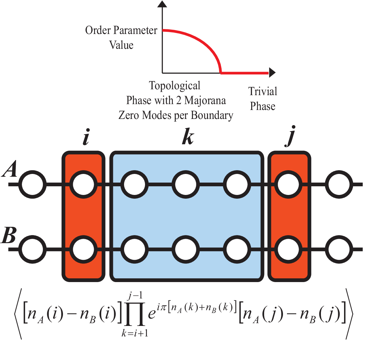
The phases of this system can be easily seen by switching to momentum $k_{y}=0,\pi$ in the transverse direction. The resulting Hamiltonian consists of two decoupled Kitaev models for the $k_{y}=0,\pi$ degrees of freedom (DOF) $\{a_{0}(i)\}_{i}\cup\{a_{\pi}(i)\}_{i}$ with modified chemical potentials $\mu_{\pm}=\mu\pm 2t_{\perp}$:

The phases of the system for $|\Delta|\neq 0$ have two, one, or zero Majorana zero modes per edge as the interchain coupling $t_{\perp}$ is increased (the phase boundaries are the same as those in Fig. 4). The phase with two Majorana zero modes per edge is protected by the exchange symmetry. To distinguish the phases we need only independently test whether the $k_{y}=0,\pi$ DOF are in the topological or trivial phases using Kitaev model string OPs. In regimes where only one of $k_{y}=0,\pi$ DOF are in the topological phase, we use string termination operators such as $\chi_{0}/\chi_{\pi}\sim\chi_{A}\pm\chi_{B}$ or those built out of $\bar{\chi}$ operators. When both $k_{y}=0,\pi$ DOF are in the topological phase, the terminating operators are for instance $\chi_{0}\chi_{\pi}\sim\chi_{A}\chi_{B}$. In other words, two copies of the topological phase OP of the Kitaev model, one each for the $k_{y}=0,\pi$ momentum DOF, detects the weakly coupled regime of this two chain system, in which each end has two Majorana zero modes. This is equivalent to a product of topological string OPs for each chain:

We take a winding path in the Jordan-Wigner mapping to transform the fermionic cylinder into a 1D infinite bosonic chain. Each bosonic unit cell accounts for one fermionic cylindrical ring and contains $N$ spin-1/2 degrees of freedom (DOF). The $\mathbb{Z}_{N}$ fermion translation symmetry for the circumference, $a_{i,j}\rightarrow a_{i,(j+1)\bmod{N}}$, maps to a $\mathbb{Z}_{N}$ symmetry internal to the unit cell, which we note is not translation of the spins. Crucially, any fermionic system also inherently must obey a $\mathbb{Z}_{2}$ fermion parity symmetry (defined as $a_{i,j}\rightarrow-a_{i,j}$), and this maps to a local $\mathbb{Z}_{2}$ symmetry of spins. Hence, the bosonic system has a $\mathbb{Z}_{2}\times\mathbb{Z}_{N}$ symmetry. To obtain fully symmetric fermionic phases, we will see that the corresponding bosonic phases may be fully or only partially symmetric.

The possible fully symmetric ($G^{\prime}=G=\mathbb{Z}_{2}\times\mathbb{Z}_{N}$) bosonic phases are found by identifying $H^{2}(\mathbb{Z}_{2}\times\mathbb{Z}_{N},U(1))$. The result depends on the parity of N, since $H^{2}(\mathbb{Z}_{2}\times\mathbb{Z}_{N},U(1))=\mathbb{Z}_{2}$ or $\mathbb{Z}_{1}$ for $N$ even or odd. To see the physical origin of this, we digress to utilize the language of matrix product states for describing wavefunctions.

In the matrix product state language,[48, 49, 50] the coefficients $C_{i_{1}i_{2}...i_{L}}$ of a wavefunction $|\psi\rangle$ in a basis $|i_{1}i_{2}...i_{L}\rangle$ are written as scalar-valued products of matrices, with each matrix indexed by $i_{k}$. For instance, for a periodic system of L sites:[50]

Next, consider a symmetry $\Sigma(g)$ of the wavefunction, with $g\in G$. The rule[36, 30] for how the matrices transform is

For our $\mathbb{Z}_{2}\times\mathbb{Z}_{N}$ symmetry, we have two bosonic generators which are in correspondence with the fermionic symmetry generators, fermion parity P and translation T. The projective representation of the two bosonic generators, labeled $U_{P},U_{T}$, each have an overall phase that can be gauge fixed, $U_{P}^{2}=U_{T}^{N}=1$. Crucially, however, the complex phase in $U_{P}U_{T}=e^{i\phi}U_{T}U_{P}$ cannot be eliminated by redefinition of the matrices $U$. Moreover, it must satisfy $e^{2i\phi}=e^{Ni\phi}=1$ because of our gauge fixing. Hence, of the two possible solutions $\phi=0,\pi$, the latter is forbidden for $N$ odd. The gauge-invariant scalar $e^{i\phi}$ is quantized and so is preserved under smooth, gap-preserving deformations to the wavefunctions. The two possible values of $e^{i\phi}$ represent two gauge-inequivalent classes of projective representations of the symmetry group $\mathbb{Z}_{2}\times\mathbb{Z}_{N}$. One can see also, that all other complex phases which cannot be gauged away are related to this one, so specifying $e^{i\phi}$ is sufficient for labeling a projective representation. Since a product state can be represented by scalar $\Gamma_{j}$ and hence scalar $U_{P},U_{T}$, $e^{i\phi}=1$ describes the trivial phase. In contrast, $e^{i\phi}=-1$ characterizes a topologically nontrivial phase.

The above analysis identifies all symmetric bosonic phases protected by $\mathbb{Z}_{2}\times\mathbb{Z}_{N}$. We must also identify some symmetry breaking bosonic phases, as they are relevant for obtaining symmetric fermionic phases. This is because, while the analog of the fermion parity symmetry P can be broken in bosonic variables, it must be restored when mapping back to fermions. It is sufficient to label these symmetry breaking bosonic phases with their unbroken symmetry subgroup $G^{\prime}\subset G$. The relevant ones are the proper cyclic subgroups generated by bosonic versions of (i) translation T and, for $N$ even only, (ii) the product of fermion parity and translation, labeled PT. We denote these by $G^{\prime}=\langle T\rangle$ and $G^{\prime}=\langle PT\rangle$ respectively. These two classes retain enough symmetry so that, although the analog of symmetry P is broken in bosonic variables, it and all other broken bosonic symmetries in $\mathbb{Z}_{2}\times\mathbb{Z}_{N}$ are restored in the fermion system. That is, the resulting fermionic phases are symmetric.

For a complementary description of the phases, we also apply the approach developed in Ref. 15 for fermions directly. On a certain subspace, fermionic symmetry operators acquire an effective form ($\hat{P},\hat{T}$) consisting of two “fractional” pieces supported on the left and right edges of the system. As with the bosonic case, it is the commutation relations of these pieces which identify the quantum phases. We elaborate on this in App. B for our case and mention the result here. If the fermionic symmetry operators acquire effective forms $\hat{P}\sim P_{L}P_{R}$ and $\hat{T}\sim T_{L}T_{R}$, where $P_{L},T_{L}$ and $P_{R},T_{R}$ are left, right fractional pieces, define $\mu,\mu^{\prime}$ so that $P_{L}P_{R}=e^{i\mu}P_{R}P_{L}$ and $T_{L}T_{R}=e^{i\mu^{\prime}}T_{R}T_{L}$. Then $e^{i\mu},e^{i\mu^{\prime}}$ are sufficient to characterize the symmetric fermionic phases.

The correspondence between the bosonic and fermionic classifications is given in Table 1. The bosonic description consists of the unbroken symmetry subgroup $G^{\prime}\subset G$ and the possible symmetry-protected topological order (“trivial” or “nontrivial”). The fermionic description consists of the commutation relations of “fractional” pieces of fermionic symmetry operators. In general, fractionalization of fermionic symmetry P into fermionic pieces ($\mu=\pi$) means it is broken in bosonic variables.[14] This is not true for other fermionic symmetries (such as our $\mathbb{Z}_{N}$ translation) whose behavior in bosonic variables depends in part on those of parity (App. B).

The fermionic operators P and T are:

We can view the set of operators $\{a_{k_{y}}(i)\}_{i}$ for fixed $k_{y}$ as degrees of freedom (DOF) for a single Majorana wire with open boundaries. For example, to construct a model for Class 3 (symmetry breaking bosonic phase with $G^{\prime}=\langle T\rangle$), we consider fixing the ground state occupations of all the $k_{y}\neq 0$ DOF (i.e. by putting all $k_{y}\neq 0$ chains into the trivial phase) so that T will act as a scalar in the ground state subspace. We treat the $k_{y}=0$ DOF instead as a topological Majorana wire. Consider:

To construct a model for Class 4 (for even N), we simply switch the treatments of the $k_{y}=0,\pi$ DOF.

We can construct a model for Class 2 (for even N) by placing both the $k_{y}=0$ and $k_{y}=\pi$ DOF into the topological phase and fixing the site occupations of the remaining $k_{y}\neq 0,\pi$ DOF. A representative model is therefore

The phases of the system can be seen by rewriting the Hamiltonian (18) as

Consequently, the phases of the system are determined by whether the independent $k_{y}=0,\pi$ DOF are in the topological phase. The $k_{y}=0$ DOF are topological when the associated chemical potential is sufficiently weak $|t_{\perp}+\frac{\mu}{2}|<|t|$. Here the 1D $\mathbb{Z}_{2}$ invariant $\nu_{k_{y}=0}=1$.[51] Likewise, the $k_{y}=\pi$ DOF are topological when $\nu_{k_{y}=\pi}=1$ for $|t_{\perp}-\frac{\mu}{2}|<|t|$. Hence, for weak $|\frac{t_{\perp}}{\mu}|$ and $|\frac{t}{\mu}|>\frac{1}{2}$ the system has two Majorana zero modes per edge, at $k_{y}=0,\pi$. This phase scales to a 2D weak TSC as $N\rightarrow\infty$ in Eq. (18), as in this regime the 2D $\mathbb{Z}$ invariant (Chern number) is $\nu=0$. For intermediate values $|t_{\perp}|\sim|t|$ and weak chemical potential the system has a single Majorana zero mode per edge (either at $k_{y}=0$ or $\pi$) and will scale to a 2D strong TSC as $N\rightarrow\infty$ since the 2D $\mathbb{Z}$ invariant $|\nu|=1$. When interchain hopping $t_{\perp}$ dominates over intrachain hopping $|\frac{t_{\perp}}{\mu}|>|\frac{t}{\mu}|+\frac{1}{2}$, the system is a weak TSC in the x-direction. Fig. 4 gives a phase diagram.

Since the three sets of DOF $k_{y}=0$, $k_{y}=\pi$, and $k_{y}\neq 0,\pi$ decouple, we can tune each into topological or trivial phases independently while maintaining translational invariance. For instance, if the $k_{y}=0$ DOF form a nontrivial state, treating this as a single chain with no other symmetries, we can find a path connecting to the model $\sum_{i}i\bar{\chi}_{0}(i)\chi_{0}(i+1)$ which preserves translation symmetry since it only involves $k_{y}=0$ operators. Hence, the quasi-1D phases of Eq. 18 – namely the 2D weak TSC associated with y-direction layering and the two strong TSCs with $(\nu_{k_{y}=0},\nu_{k_{y}=\pi})=(1,0)$ or $(0,1)$ – would fall into Classes 2, 3, and 4, respectively, of our classification. It appears that for free fermions our classification identifies the 1D $\mathbb{Z}_{2}$ invariants $\nu_{k_{y}=0}$ and $\nu_{k_{y}=\pi}$ and consequently $\nu\bmod 2$ since $\nu_{k_{y}=0}+\nu_{k_{y}=\pi}=\nu\bmod 2$. [51]

The weak TSC with $\nu_{k_{x}}\neq 0$ for $k_{x}=0$ or $\pi$, which is associated with layering in the x-direction, appears as a trivial phase. This phase results with strong $t_{\perp}$, but in the momentum $k_{y}$ basis this coupling is an effective chemical potential, $\mu_{\pm}=\mu\pm 2t_{\perp}$, which favors on-site pairing of y-momentum Majoranas, driving the $k_{y}=0,\pi$ Majorana chains away from nontrivial pairing. It is natural that that our classification is unable to detect the topological index associated with x-translation symmetry along the cylinder length, as only y-translation has been included.

In fact, this conclusion can be false if one stays away from the system boundary in applying the symmetry over a large domain. This is because applying a symmetry over some region creates an “artificial” boundary, in a certain sense, and different topological phases have distinct edge states which are “created” at this artifical edge.[30] The bosonic selection rules[30] tell us that the operators $O_{L,R}$ which terminate the bosonic string (fermionic brane) can be chosen to transform under symmetries in such a way as to select a quantum phase. The distinction between the two phases Classes 1 and 2 in the bosonic description is the quantity $e^{i\phi}=\pm 1$ (Sec. III). $O_{L,R}$ must be even under parity (because it is the symmetry used in the bulk of the order parameter) but transform as $e^{i\phi}$ under translation in order to be finite in the quantum phase labeled by $e^{i\phi}$. The OP is guaranteed to vanish in the other symmetric bosonic phase. Mapped back to the fermionic system, the brane termination operators should be bosonic but should be even or odd under translation so that the OP is nonzero in Classes 1 or 2, respectively.

$S_{1}$ is, for instance, an order parameter which is nonzero in Class 1 but vanishes in Class 2 since translation invariant operators terminate its bulk. To construct a candidate with reversed behavior, we can choose operators such as $O(i)=i\chi_{0}(i)\chi_{\pi}(i)$ or $i\bar{\chi}_{0}(i)\bar{\chi}_{\pi}(i)$, which are parity invariant but translation odd, to terminate the fermionic brane. Hence, candidate order parameters which give a nonzero value for Class 2 only include

Finally, we utilize the fact that certain symmetries are broken in the bosonic variables to construct OPs that are nonzero in a symmetry breaking bosonic phase but vanish elsewhere. We use two-point functions in the bosonic variables $\langle U_{i}V_{j}\rangle$ with $|i-j|\rightarrow\infty$; if $U,V$ are odd under P but even under T, the result is nonzero in Class 3 but vanishes in the other symmetric fermionic phases. Likewise, operators odd under P but even under PT yield OPs which can detect Class 4. Mapped back to fermions, a few such candidates are:

References

- [1] J. Alicea, Rep. Prog. Phys. 75 (2012).
- [2] V. Mourik, K. Zuo, S. Frolov, S. Plissard, E. Bakkers, and L. Kouwenhoven, Science 336, 1003 (2012).
- [3] M. Deng, C. Yu, G. Huang, M. Larsson, P. Caroff, and H. Xu, Nano Lett. 12, 6414 (2012).
- [4] A. Das, Y. Ronen, Y. Most, Y. Oreg, M. Heiblum, and H. Shtrikman, Nature Physics 8, 887 (2012).
- [5] L. P. Rokhinson, X. Liu, and J. K. Furdyna, Nature Physics 8, 795 (2012).
- [6] H. Churchill, V. Fatemi, K. Grove-Rasmussen, M. Deng, P. Caroff, H. Xu, and C. Marcus, Phys. Rev. B 87, 241401 (2013).
- [7] A. Finck, D. Van Harlingen, P. Mohseni, K. Jung, and X. Li, Phys. Rev. Lett. 110, 126406 (2013).
- [8] A. Kitaev, arXiv:cond-mat/0010440.
- [9] N. Read and D. Green, Phys. Rev. B 61, 10267 (2000).
- [10] X.-L. Qi, T. L. Hughes, S. Raghu, and S.-C. Zhang, Phys. Rev. Lett. 102, 187001 (2009).
- [11] A. P. Schnyder, S. Ryu, A. Furusaki, and A. W. W. Ludwig, Phys. Rev. B 78, 195125 (2008).
- [12] A. Kitaev, in Proceedings of the L.D. Landau Memorial Conference ‘Advances in Theoretical Physics’ (2008), arXiv:0901.2686.
- [13] L. Fidkowski and A. Kitaev, Phys. Rev. B 81, 134509 (2010).
- [14] L. Fidkowski and A. Kitaev, Phys. Rev. B 83, 075103 (2011).
- [15] A. M. Turner, F. Pollmann, and E. Berg, Phys. Rev. B 83, 075102 (2011).
- [16] F. Burnell, X. Chen, L. Fidkowski, and A. Vishwanath, arXiv:1302.7072.
- [17] L. Fidkowski, X. Chen, and A. Vishwanath, Phys. Rev. X 3, 041016 (2013).
- [18] X. Chen, L. Fidkowski, and A. Vishwanath, arXiv:1306.3250.
- [19] C. Wang and T. Senthil, Phys. Rev. B 87, 235122 (2013).
- [20] C. Wang, A. C. Potter, and T. Senthil, Phys. Rev. B 88, 115137 (2013).
- [21] X. Chen, Z.-C. Gu, and X.-G. Wen, Phys. Rev. B 84, 235128 (2011).
- [22] X. Chen, Z.-C. Gu, Z.-X. Liu, and X.-G. Wen, arXiv:1106.4772.
- [23] X. Chen, Z.-C. Gu, Z.-X. Liu, and X.-G. Wen, Science 338, 1604 (2012).
- [24] N. Schuch, D. Perez-Garcia, and I. Cirac, Phys. Rev. B 84, 165139 (2011).
- [25] Z.-C. Gu and X.-G. Wen, arXiv:1201.2648.
- [26] Y.-M. Lu and A. Vishwanath, Phys. Rev. B 86, 125119 (2012).
- [27] A. Vishwanath and T. Senthil, Phys. Rev. X 3, 011016 (2013).
- [28] C. Wang, A. C. Potter, and T. Senthil, Science 343, 629 (2014).
- [29] J. Haegeman, D. Perez-Garcia, I. Cirac, and N. Schuch, Phys. Rev. Lett. 109, 050402 (2012).
- [30] F. Pollmann and A. M. Turner, Phys. Rev. B 86, 125441 (2012).
- [31] M. Zaletel, arXiv:1309.7387.
- [32] M. den Nijs and K. Rommelse, Phys. Rev. B 40, 4709 (1989).
- [33] T. Kennedy and H. Tasaki, Phys. Rev. B 45, 304 (1992).
- [34] M. Oshikawa, J. Phys.: Condens. Matter 4, 7469 (1992).
- [35] M. Endres, M. Cheneau, T. Fukuhara, C. Weitenberg, P. Schauss, C. Gross, L. Mazza, M. Banuls, L. Pollet, I. Bloch, et al., Science 334, 200 (2011).
- [36] D. Perez-Garcia, M. M. Wolf, M. Sanz, F. Verstraete, and J. I. Cirac, Phys. Rev. Lett. 100, 167202 (2008).
- [37] F. Anfuso and A. Rosch, Phys. Rev. B 76, 085124 (2007).
- [38] E. Berg, E. G. Dalla Torre, T. Giamarchi, and E. Altman, Phys. Rev. B 77, 245119 (2008).
- [39] F. Pollmann, E. Berg, A. M. Turner, and M. Oshikawa, Phys. Rev. B 85, 075125 (2012).
- [40] W. Bakr, J. I. Gillen, A. Peng, S. Fölling, and M. Greiner, Nature 462, 74 (2009).
- [41] W. Bakr, A. Peng, M. Tai, R. Ma, J. Simon, J. Gillen, S. Fölling, L. Pollet, and M. Greiner, Science 329, 547 (2010).
- [42] E. Alba, X. Fernandez-Gonzalvo, J. Mur-Petit, J. K. Pachos, and J. J. Garcia-Ripoll, Phys. Rev. Lett. 107, 235301 (2011).
- [43] E. Zhao, N. Bray-Ali, C. J. Williams, I. B. Spielman, and I. I. Satija, Phys. Rev. A 84, 063629 (2011).
- [44] N. Goldman, E. Anisimovas, F. Gerbier, P. Öhberg, I. Spielman, and G. Juzeliūnas, New J. Phys. 15, 013025 (2013).
- [45] H. M. Price and N. R. Cooper, Phys. Rev. A 85, 033620 (2012).
- [46] M. Atala, M. Aidelsburger, J. T. Barreiro, D. Abanin, T. Kitagawa, E. Demler, and I. Bloch, Nature Physics 9, 795 (2013).
- [47] E. G. Dalla Torre, E. Berg, and E. Altman, Phys. Rev. Lett. 97, 260401 (2006).
- [48] M. Fannes, B. Nachtergaele, and R. Werner, Commun. Math. Phys. 144, 443 (1992).
- [49] G. Vidal, Phys. Rev. Lett. 91, 147902 (2003).
- [50] G. Vidal, Phys. Rev. Lett. 98, 070201 (2007).
- [51] D. Asahi and N. Nagaosa, Phys. Rev. B 86, 100504 (2012).
- [52] M. Kohmoto, M. den Nijs, and L. P. Kadanoff, Phys. Rev. B 24, 5229 (1981).
- [53] M. Yamanaka and M. Kohmoto, Phys. Rev. B 52, 1138 (1995).
- [54] W. Son, L. Amico, and V. Vedral, Quantum Information Processing 11, 1961 (2012).