A local constant-factor approximation algorithm for MDS problem in anonymous network
Abstract
In research on distributed local algorithms it is commonly assumed that each vertex has a unique identifier in the entire graph. However, it turns out that in case of certain classes of graphs (for example not lift-closed bounded degree graphs) identifiers are unnecessary and only a port ordering is needed [8]. One of the open issues was whether identifiers are essential in planar graphs. In this paper, we answer this question and we propose an algorithm which returns constant approximation of the MDS problem in model. The algorithm doesn’t use any additional information about the structure of the graph and the nodes don’t have unique identifiers. We hope that this paper will be very helpful as a hint for further comparisons of the unique identifier model and the model with only a port numbering in other classes of graphs.
0.1 Introduction
In recent years, there has been a growing interest in designing distributed local algorithms. It might come out of the easiness of applying these algorithms in reality. They run very fast (in constant time) and are tolerant to the network structure changes and node failures. It turns out the running time of these algorithms is completely decoupled from the size of the network and each node takes its decision based only on the knowledge about its k-neighbourhoods. This fact is very important for the scalability of an algorithm in large networks. If the structure of the network changes (i. e. a vertex is removed), then an algorithm must be re-called to repair a solution only for a small surrounding of the removed vertex. It is a significantly faster solution than in case of standard algorithms requirements, which require re-execution of the algorithm on the entire network.
In some research on designing local algorithms(but not strictly local), it is allowed that nodes have a knowledge about the -neighbourhood, where is a function that depends on the number of vertices in the network. However, in this paper we only consider strictly local algorithms, that do not need any additional information about the structure of the graph and don’t have unique identifiers, so they satisfy much stronger assumptions.
In recent years, several deterministic distributed local algorithms have been proposed. They return solutions that are good approximations of various problems (e.g. minimum edge cover, minimal dominating set[12], semi-matching[6, 7]), in constant time in different classes of graphs (e. i. bounded degree graphs, planar graphs). However, these algorithms very often assume that nodes have unique identifiers. This assumption could be very important if we consider a more ”real” model, in which in a single communication round, each vertex can send a message which contains at most bits, where is the number of vertices in the graph. This limitation makes it impossible to e.g. detect small cycles in the network, gather knowledge of 2-hop neighbourhoods. Recently in a paper [8] the authors Göös et al. have shown that for lift-closed bounded degree graphs, a model with unique identifiers (known as [14]) and model with a port numbering only(known as PO model[8]), are practically equivalent. However, techniques used in their work do not allow us to consider the equivalence of these models for Minimum Dominating Set() problem in planar graphs. It is known[12] that there exists an algorithm for planar graphs which, in constant time, returns a constant approximation of the in model with unique identifiers and an unbounded message size.
It turns out that there also exists a strictly local algorithm for planar graphs, that in the model without unique identifiers and with upper bounded message size, finds constant approximation of the Minimum Dominating Set.
0.1.1 Related Work
A distributed algorithm is called a local algorithm if it completes in a constant number of synchronised communication rounds. If we assume that the nodes do not have any additional information about the other vertices, then we say that our algorithm is strictly local.
The research on local algorithms has been ongoing for several years ([1, 3, 9, 14, 15, 16, 17]), but the strictly local algorithms gained the increased interest just recently. There are now more than one hundred works referring, more or less closely, to the topic of such algorithms. Thus, it is not possible to briefly describe all of these publications. The best way to study this topic is to read excellent survey[18] written by Suomela. That article describes all the important results obtained so far by all the researchers. One of many open questions is an issue raised in a paper [8] concerning the similarity of two models: a model with unique identifiers and a model with only a port numbering for MDS problem in planar graphs. We answer this question.
One of the first papers, that considered network without unique identifiers, has been written by Angluin [2]. Unfortunately, in 1992, Linial showed in [14] that there is no algorithm that, in constant time, finds a Maximal Independent Set in a cycle in the unique identifiers model. This result shows how difficult it is to find a fast distributed algorithm and it is even more difficult if we consider strictly local algorithms only. Thankfully, in 1995 Naor and Stockmeyer in [16] introduced the concept of Local Checkable Labelling() problems and showed that if there is a local algorithm in a model with unique identifiers on nodes then there is also order-invariant local algorithm which uses only the fact that for each pair of vertices or . So from the point of view of the problems both models are almost equivalent. Note that the class of problems contains among others the maximal independent set or vertex colouring. Thus, a natural question then came up, whether there exists an algorithm which, without information about the sequence of vertices is able to solve any non-trivial problem. Kuhn and Wattenhofer in [11], presented the first local but randomized algorithm for bounded degree graphs. Their algorithm does not require long messages. Then in [10] the algorithm has been improved by Kuhn et al. Notice that both approaches used the method of linear programming. The first local algorithm for MDS problem for planar graphs was proposed by Lenzen et al. in [12], but their algorithm requires long messages and unique IDs on nodes.
There is also a lower bound for possible approximation factor of an algorithm. In [4] it has been shown that there is no algorithm which in a constant number of communication rounds returns an approximation of the MDS in planar graphs.
0.1.2 Main Results and Organisation
Our main result is summarised in the following theorem. Let denote an arbitrary MDS in a planar graph .
Theorem 1.
Let be a planar graph and be a set returned by algorithm PortNumberingMds. Then
The rest of this paper is structured as follows. We begin by describing the computational model and notation used in this paper. Then in section 0.2.1 we briefly introduce the principle of our algorithm and its formal pseudocode. Next, in section 0.2.2, we present the analysis of the correctness of our algorithm, and compute the approximation factor of the algorithm. At the end, in section 0.3, we summarise our considerations.
0.1.3 Model and Notation
In this paper we work in a synchronous communication model and as a representation of the network we use a planar graph . Edges in the graph will correspond to communication links and processors will correspond to vertices from the set . Moreover, we assume that each vertex has its own labelling of its incident edges and vertices do not have unique identifiers and also do not have any additional information.
In order to facilitate the reader to understand this paper, we use the same notations as in [12]. For nodes we define the set of inclusive neighbourhood of as . We also denote the neighbours of not in as . To simplify the notation in cases where we may omit the braces, e.g. instead of .
0.2 Constant approximation in model
0.2.1 Algorithm
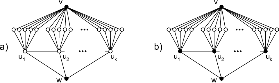
The key idea of the algorithm is based on an appropriate use of planarity of the graph . Intuitively, some vertex should belong to the dominating set if it dominates a lot of its neighbours. However, in reality, such approach does not give a constant approximation as we can see in the Figure 7. This situation occurs if graph contains many vertices with big common neighbourhood. In our algorithm we first dominate only a small subset of these vertices (step 2 and 3 of the algorithm). So we avoid unnecessary adding of multiple vertices which dominate the same or almost the same neighbourhoods.
In the next round each vertex not dominated yet adds to the set a dominated vertex with biggest residual degree from its dominated neighbourhood. The planarity of the graph ensures that there is a small number of such added vertices. To prove that both sets are small, we will use well known fact that Jordan curve divides the plane into two regions - an interior and an exterior, so that any cycle in a planar graph divides the graph into two parts without edges between their interiors. We partition our plane graph into disjoint regions in such way that the number of regions are proportional to the size of the set and moreover, in each region there is at least one vertex from the set .
0.2.2 Analysis
As can be easily seen, the algorithm can be performed in a constant number of communication rounds and returns a dominating set due to last round (step 9), where all not dominated vertices add exactly one of their neighbours to the dominating set . Therefore, in our analysis we only need to show that the numbers of vertices added to the dominating set in steps 2, 3 and 9 are small enough that our algorithm returns solutions which are a constant approximation of an optimal MDS. To simplify notation in our analysis, we assume that the set of vertices added in step 2, 3 and 9 will be denoted by , and respectively, and some fixed optimal solution will be denoted as . We need to recall the following well-known lemma.
Lemma 1.
A minor of a planar graph is planar. A planar graph of nodes has less than edges. A planar bipartite graph of nodes has less than edges.
We will begin the analysis of our algorithm with estimating the maximal number of vertices added to the set . To bound this value we need to define a special subgraph of graph .
Definition 1.
Let graph be a subgraph of constructed in the following way:
- i)
and , where is a set from step 2 of the algorithm.
- ii)
Add all edges between vertices from .
- iii)
Add minimal number of edges (from ) and nodes (from ) such that each vertex from the current set has adjacent vertex from the set or is contained in the set (so for each we have ).
In order to simplify the description of proofs, we will also introduce the following notation (see Figure 1):
where is a vertex chosen in the step 10 of the algorithm. Notice that not all of the subsets are disjoint, for example, it is possible that some fixed vertex belongs to both sets and ().

To show that the maximal number of vertices in the set is comparable to the order of the set , we will consider the size of each set , , and separately. This analysis is contained in Lemma 2, Lemma 3 and Lemma 7.
At the beginning we will prove, a simple but very useful fact.
Fact 1.
Proof.
Note that the vertex from the set has been added in step 2 of the algorithm by one of the vertices in . In addition, each vertex adds at most one vertex to . Thus, the order of the set cannot be greater than the order of the set . ∎
Lemma 2.
Proof.
The set is a set contains the elements which both belong to sets and . Hence the order of is less or equal to the order of (). Moreover, using Fact 1, we obtain that . ∎
Lemma 3.
Proof.
In the step 2 of the algorithm every vertex adds its adjacent vertex with the biggest residual degree (where ) from the inclusive neighbourhood. The definition of the set implies that every vertex that does not belong to has at least one neighbour in the set , so that vertices from the set have to be dominated in the optimal solution . Let us define a set then for all we have that the residual degree of is less or equal to (). Otherwise, the vertex would not belong to () because its residual degree is bigger than . Hence, every vertex dominates at most vertices from the set so . Using from Fact 1, we obtain that . ∎
Our goal is to show that so it is left to prove that the maximal number of vertices in is small (). For this purpose, we will use a technique of splitting the graph into bunches and then we will show that each induced region of a bunch contains many vertices from the set . We start by defining what we mean by a term bunch, which was first introduced in [5].
Definition 2.
Let be a planar graph, , and . A --path is called S-T-W-special if it has the form , where , and .
Although our algorithm works in planar graphs, in the analysis we assume that the given graph is plane. Let us recall some basic theoretical graph terminology for planar graphs. If is a plane graph in then maximal open set in such that any two points in can be connected by a curve contained in is called a face of . Let be two special --paths. In any plane drawing, graph contains exactly one bounded face. (We will assume here that the face is empty if .) Now we set and where is the bounded face in the drawing of .
Definition 3.
Let be a plane graph and let , where . A maximal set of S-T-W-special paths between and is called a S-T-W-bunch between and if there exist two distinct paths such that all paths from are contained in and no vertex from is contained in . In addition, the paths will be called the boundary paths of . Moreover if a bunch contains at least five special paths then we say that is a large bunch.
To simplify the notation, if the sets , , are clear from the context, we will write special paths instead of A-B-C-special paths. In one of the last lemmas in this paper we will consider special paths and bunches of length three. Their definition is analogous to the definitions of bunches with special paths of length two.
After defining the concepts of bunches and special paths, next, in Fact 3 and Lemma 7, we will estimate their sizes. Then, in Lemma 6, we will show that most of regions designated by the bunches contain many vertices from the set . The proof of Fact 3 is quite complicated and at the beginning we show that the number of connected components of the induced subgraph is smaller than .
Lemma 4.
Let be a graph and be a dominating set in . If is a subgraph of such that and every vertex contains at least one adjacent vertex from then
Proof.
Let be a partition of to minimal number of connected components. If a set contains at least one vertex then there is a vertex such that . Hence each connected component contains at least one vertex from . In other case there is no vertex in component then since thus contains at least one vertex from a set . We obtain that each connected component contains at least one vertex from thus . ∎
Lemma 5.
Let be a planar graph and be subsets of vertices such that the sets are pairwise disjoint and each vertex from is adjacent to at least one vertex from each sets and . Then graph contains at most ---bunches, where denote the number of connected components in graph .
Proof.
To bound the number of bunches in the graph more effort is required. First of all, we need to define a multigraph obtained from by contracting each vertex to any adjacent vertex and adding edge between contracted vertices and neighbours of a vertex from a set (see Figure 2). Let vertices was contracted in the graph then we say that path from the graph (, , ) corresponds to edge in the graph . Notice that each vertex is adjacent with exactly one vertex .

Let us consider a connected component of the multigraph (), where denotes the set of all vertices from such component. Then we can find spanning tree in a multigraph . From a well known Lemma 1 we know that a multigraph is planar.
Consider a plane drawing of . Let for every vertex and define a ball around a vertex of radius , such that intersects only with these edges of that contain and does not contain points from other balls. We denote a connected region of as a side of vertex . It is obvious that every edge from that contains reaches by some side of a vertex . In this case we will say the edge ends in side (see Figure 3).

We also have to prove similar fact like in paper [5].
Fact 2.
The multigraph contains at most two edges of such that and end in the same sides and corresponding special paths of edges in belong to different A-B-C-bunches in corresponding graph , where denotes all contracted vertices in . Furthermore there is at most one such pair of edges in a multigraph .
Proof.
Let F be the set of - edges from that end in the same sides of and . Assume that belong to different bunches then is a cycle and consequently every other - edge i.e. must be contained in one of the regions of . Because corresponding special paths of and are contained in different bunches in thus the region where contains all vertices from . If there is other - edge which belongs to different bunch than and contained in the bounded face of or bounded face then there is a vertex from the set which is contained in the bounded region of the cycle . Then e,e’ and e” end in different side of u (contradiction). Moreover if graph contains such edges then from planarity there is no any other pair of edges which ends in the same sides of two vertices. ∎

Let be the supergraph of obtained as follows. For every vertex put a vertex in each side of and join it with by one edge. The set of new added vertices we denote as . Substitute the edge from which ends in the side of containing with the edge that ends in . Let be a maximal set of edges which corresponds to special paths in some fixed bunch from then we remove edges from . The supergraph is a planar multigraph and using Fact 2 we obtain that almost every pair of vertices (except for one) could be connected by at most one edge from a set . Let us notice that for each bunch in there exists disjoint corresponding edge in . For every vertex we add exactly new vertices, thus we can simply determine the number of new added vertices from a supergraph
| (1) |
Let us observe that in our lemma we consider ---bunches, where sets , , are pairwise disjoint. Thus each special path of considered bunches has one endpoint in set and one in . Hence we may assume that our supergraph is bipartite. Using Lemma 1, Fact 2 and equation (1) we obtain that number of edges
| (2) |
Notice that edges between vertices from a spaning tree and new vertices was added in supergraph but not exists in and moreover some edges (i.e. ) belong to the same bunch. We can omit such edges in our calculation, thus the maximal number of bunches in the graph is less than . Unfortunately, the graph may not be connected, therefore the number of bunches may be greater than due to some bunch could be contained in a region of other bunch . If we consider creating a multigraph by sequentially adding connected components then in -th step after adding corresponding component we create at most new bunches. So a graph contains at most bunches.
∎
Fact 3.
Let , and . Then the graph contains at most A-B-C-bunches. This set of bunches we denote by .
Lemma 6.
Let be a bunch such that contains at least five ---special paths in the graph (). Then , where and , are boundary paths of a bunch .
Proof.
Let us consider the structure of a subgraph of induced by vertices contained in a region designated by a boundary of special paths of some bunch (). Recall that we denote a number of special paths in a bunch as and we take into account only bunches such that . Hence each considered bunch contains a vertex , a vertex and at least five vertices from the set (see Figure 5). Moreover, a bunch creates at least disjoint regions in the graph . We will show that many of them contain vertices from and, more precisely, each region contains at least vertices from .

Since vertex belongs to the set , thus was added to by some vertex in the step 5 of the algorithm, as a vertex with the largest degree in the neighbourhood . It is possible that but note that a vertex can add only one such vertex. Let us assume that . Using an assumption that we obtain thus an interior vertex (see Figure 5) could not have been added by any of the vertices , or until some other node adjacent to exists in , , (see Figure 5). Hence each interior vertex is adjacent with at least one vertex from region such that at least one of the following cases is satisfied or
- a)
- b)
such that and
Let be a set of vertices lying inside and adjacent to a vertex . Suppose that and case a) is not satisfied for any , so and . In the optimal solution every vertex belongs to or has a neighbour in this set, thus there exist vertices such that each dominates (). Recall that there exists such that (determined in step 4 of the algorithm) so . Assume by contradiction, that case b) is also not satisfied for each . Then , but in this case and thus there is no vertex such that . It is a contradiction with assumption that . Hence at least one of the cases a), b) is satisfied.
In a subgraph induced by boundary paths of a bunch there are exactly internal vertices from the set and furthermore at most one such vertex could be chosen by vertex from this bunch. So at least internal vertices of the bunch have corresponding vertex which is contained in the region . Notice that it is possible that two vertices have corresponding vertices in the same face (i.e ). Thus, we get that . ∎
Now we are ready to show that the .
Lemma 7.
Let and be constants such that
Proof.
We start with an outline of the proof. Our goal is to show that . To this end, we first prove that there are many of edges in the set ( was specified in Definition 1 on page 1). Since is large set, the graph contains also many ---bunches. In addition using Lemma 6, most of them contain a lot of vertices from the optimal solution . Hence, finally we get that .
Assume that (where ). In other case lemma is proved because . To estimate the order of the set of edges we will first consider number of edges in sets and in a graph . Notice that the graph is planar and sets and are disjoint (). Hence, from the assumption that and Lemma 1 and Lemma 2 we get that
Notice also that set is empty (). Indeed, if there is an edge such that and then vertex would have chosen vertex , so would not be in the set (). Let be a subset of , where no edge has two endpoints inside set. Thus using planarity we obtain the following inequality From the definition of the set we know that each vertex is adjacent to at least vertices from . Hence,
Observe that there is a bijection from to a set of ---special paths in the graph . Thus a graph contains at least special paths.
Now we would like to use fact 3 and lemma 6 together. To do it we have to ensure that considered bunches contain at least five special paths (assumption of the lemma 6). Recall that if bunch contains at least five special paths then we say that is large. It is obvious from pigeonhole principle, that there are at most special paths which do not belong to large bunches.
Now we will calculate order of the set of ---special paths in graph which belong to the set of large bunches. From Fact 3 we know that , so at most considered special paths not belong to a set of large bunches. Let be a set of special paths which are contained in some large bunch and such that a internal vertex of each special path was not added to set by a vertex then
Using lemma 6 and observing that in calculation of a set we remove four vertices for each bunch we get that
∎
Notice that using easily lemmas 2, 3, and 7 and assuming proper values for constants and we obtain that and moreover using exactly the same reasoning we could prove following lemma.
Lemma 8.
Let , and be defined as in earlier lemmas. Then
Thus to prove that our algorithm returns a constant approximation of the MDS problem we have to show that . Let us observe that the set contains only vertices which are not dominated by set . We divide a set to three pairwise disjoint subsets , , and . The orders of the sets and is obvious so we only have to calculate the size of the set .
Our last step is to prove that .
Definition 4.
Let graph be a subgraph of constructed in the following way:
- i)
and .
- ii)
For every vertex add exactly one vertex . The set of added vertices denote as . Add also edge to .
- iii)
Add minimal number of edges (from ) and nodes (from ) such that each vertex has adjacent vertex from the set .
- iv)
Add minimal number of edges (from ) and nodes (from ) such that each vertex has adjacent vertex from the set .

Notice that cannot be adjacent to any vertex from a set , indeed in other case a vertex would be dominated by and so it will omit a step 10 of the algorithm.
Fact 4.
Let denote a set of ----bunches in graph as . Then
Proof.
To prove this lemma we need to observe that sets , , , and in graph are pairwise disjoint. Moreover each vertex has exactly one adjacent vertex . Thus if be a graph constructed from by contracting each such edge then we apply this graph in Lemma 5 and obtain that ∎
Lemma 9.
Let be a bunch such that contains at least five ----special paths in graph (). Then
Proof.
The graph induced by vertices contained in a region of some bunch () looks quite similar like a bunch from a set . Using the same reasoning as in the corresponding Lemma 6 we will obtain that for every vertex there exists at least one vertex inside adjacent to such that at least one following case is satisfied:
- a)
- b)
such that , and
A vertex was added to the set in the step 9 by vertex thus
Hence for each an interior vertex there exist adjacent vertices which are not dominated by any vertex . Suppose that and case b) is not satisfied then vertices must be adjacent with single vertex . Let us notice that vertex is adjacent with at least one vertex so . Contradiction that vertex chose in the step 10 of the algorithm. Each internal vertex from a bunch has a corresponding vertex which is contained in one of two surrounding faces. Since two vertices could share the same corresponding vertex thus we obtain that . ∎
Lemma 10.
Proof.
Let us notice that for any and there is no edge in a graph . Indeed, in other case a vertex will be dominated in step 2 or step 3 of the algorithm so would not belongs to a set . Moreover every vertex must be dominated in so must be adjacent to some vertex . If we denote a set of special paths which are contained in set of large bunches as then So similarly like in a lemma 6 we get that
∎
Theorem 2.
Let be a planar graph and be a set returned by the algorithm PortNumberingMds and be an optimal solution of the Minimum Dominating Set for a given graph then
Proof.
Let us fix values of constants and in the following way . Then value of from earliest lemma is equal to . We know that the order of the set returned by our algorithm satisfy a following inequality
0.3 Conclusion
In this paper we presented a constant approximation algorithm for the MDS problem in planar graphs. The algorithm is deterministic and strictly local. So nodes do not need any additional information about the structure of the graph and don’t have unique identifiers. In our algorithm we use only short messages with at most bits ( model).
Recently in paper ”Lower Bounds for Local Approximation”[8] Mika Göös et al. have shown that for lift-closed bounded degree graphs models PO and ID are practically equivalent. In this paper we show that it is true for planar graphs and MDS problem. We hope that this work will be very helpful as a hint for further comparisons of these models in other classes of graphs.
References
- [1] N. Alon, L. Babai, and A. Itai. A fast and simple randomized parallel algorithm for the maximal independent set problem. Journal of Algorithms, 7(4):567–583, 1986.
- [2] D. Angluin. Local and global properties in networks of processors. In Proc. 12th Annual ACM Symposium on Theory of Computing (STOC, Los Angeles, CA, USA, April 1980), pages 82–93. ACM Press, New York, NY, USA, 1980.
- [3] R. Cole and U. Vishkin. Deterministic Coin Tossing with Applications to Optimal Parallel List Ranking. Information and Control, 70(1):32–53, 1986.
- [4] A. Czygrinow, M. Hanćkowiak, and W. Wawrzyniak. Fast distributed approximations in planar graphs. In Proc. 22nd International Symposium on Distributed Computing (DISC, Arcachon, France, September 2008), volume 5218 of Lecture Notes in Computer Science, pages 78–92. Springer, Berlin, Germany, 2008.
- [5] A. Czygrinow, M. Hanćkowiak, and W. Wawrzyniak. Distributed packing in planar graphs. In the twentieth ACM Symposium on Parallel Algorithms and Architectures, pages 55–61, 2008.
- [6] A. Czygrinow, M. Hanćkowiak, K. Krzywdzinski, E. Szymańska, and W. Wawrzyniak. Brief announcement: Distributed approximations for the semi-matching problem. In Proc. 25th International Symposium on Distributed Computing (DISC, Rome, Italy, September 2011), volume 6950 of Lecture Notes in Computer Science, pages 200-201. Springer,Berlin, Germany, 2011.
- [7] A. Czygrinow, M. Hanćkowiak, E. Szymanska, and W. Wawrzyniak. Distributed 2-approximation algorithm for the semi-matching problem. In Proc. 26th International Symposium on Distributed Computing (DISC, Salvador, Brazil, October 2012), volume 7611 of Lecture Notes in Computer Science, pages 210-222. Springer, Berlin, Germany, 2012.
- [8] M. Göös, J. Hirvonen, and J. Suomela , Lower Bounds for Local Approximation, In Proc. 31st Annual ACM Symposium on Principles of Distributed Computing (PODC, Madeira, Portugal, July 2012), pages 175–184. ACM Press, New York, NY, USA, 2012.
- [9] A. Israel and A. Itai. A fast and simple randomized parallel algorithm for maximal matching. Information Processing Letters, 22(2):77–80, 1986.
- [10] F. Kuhn, T. Moscibroda, and R. Wattenhofer. The price of being near-sighted. In Proc. 17th Annual ACM-SIAM Symposium on Discrete Algorithms (SODA, Miami, FL, USA, January 2006), pages 980–989. ACM Press, New York, NY, USA, 2006.
- [11] F. Kuhn and R. Wattenhofer. Constant-time distributed dominating set approximation. Distributed Computing, 17(4):303–310, 2005.
- [12] C. Lenzen, Y. A. Oswald, and R. Wattenhofer. What can be approximated locally? TIK Report 331, ETH Zurich, Computer Engineering and Networks Laboratory, November 2010.
- [13] C. Lenzen and R. Wattenhofer. Leveraging Linial’s locality limit. In Proc. 22nd Symposium on Distributed Computing (DISC 2008), volume 5218 of LNCS, pages 394–407. Springer, Berlin, 2008.
- [14] N. Linial. Locality in Distributed Graph Algorithms. SIAM Journal on Computing, 21(1):193–201, 1992.
- [15] M. Luby. A Simple Parallel Algorithm for the Maximal Independent Set Problem. SIAM Journal on Computing, 15(4):1036–1055, 1986
- [16] M. Naor and L. Stockmeyer. What Can Be Computed Locally? SIAM Journal on Computing, 24(6):1259–1277, 1995.
- [17] D. Peleg. Distributed Computing: A Locality-Sensitive Approach. Society for Industrial and Applied Mathematics, Philadelphia, PA, USA, 2000.
- [18] J. Suomela, Survey of local algorithms. ACM Computing Surveys (to appear), http://www.cs.helsinki.fi/local-survey/