Cosmological perturbation theory
Abstract
The purpose of these lectures is to give a pedagogical overview of cosmological perturbation theory, following the lectures given during the school. The topics treated are:
I – The background
II – Scalar/Vector/Tensor decomposition and the gauge issue
III – The example of the tensor modes
IV – Density fluctuations, transfer function and power spectrum
V – Initial condition theory: quantum vacuum fluctuations
Most of the material presented here is available in many well-written reviews or textbooks, so in order to avoid unnecessary heavy presentation as well as to make sure I forget nobody, I will only cite the review paper Mukhanov et al. (1992) as well as the book Peter and Uzan (2013) from which most of the figures have been taken. Useful extra information and different perspectives can be also found in Lemoine et al. (2008) (in particular the review articles by A. Linde on inflation, J. Martin on the quantum aspect of initial condition and their subsequent squeezed evolution and C. Ringeval on the numerical evolution of perturbations). Ref. Weinberg (2008) provides a personal vision of S. Weinberg with many original proofs to well-known results, and Mukhanov (2005) describes in more details the relevant physics for calculating the quantities actually to be compared with the data. Finally, all numerical figures are taken from the Particle Data Group Beringer et al. (2012) whose latest update is always available on the linked site.
Keywords:
Cosmology, Inflationary cosmology, Alternative to InflationClassification:
98.80.-k,98.80.Cq1 Introduction: the background
Even though these lectures concern cosmological perturbation theory, I felt an introduction to the background could be welcome, would it be only to fix the notations, set the framework and make apparent what the problems and questions are.
Cosmology is the part of physics that studies the Universe as a whole, trying to make models of its overall evolution and its structure. As such, it is a quite peculiar branch of physics, as by definition there is only one Universe – hence the name – and it is impossible to make any experiment on either its evolution or structure! From these considerations, we immediately see that cosmology will be endowed with various intrinsic limitations which I will discuss in due turn.
How do we, practically, describe cosmology? To begin with, one needs a theoretical framework providing the evolution equations. This will be general relativity: the Universe will be seen as a 4-dimensional manifold, space-time, endowed with a metric whose dynamics follows from Einstein equations
| (1) |
where , the velocity of light in vacuum, will be set to unity in all further calculations (along with where it should have appeared in the final section of these lectures), is Newton’s constant, is the stress-energy tensor of the matter – discussed later – and the cosmological constant. We know from observations that the latter is probably not vanishing, contrary to what was supposed until recently, but we can however consider its influence as another matter fluid and include it in . Therefore, one can, without lack of generality, send in Eq. (1).
The Einstein tensor is defined in terms of the Ricci tensor and scalar , the former stemming from a contraction of the Riemann tensor through . Finally, the relation with the metric itself is made with the definition
| (2) |
and the Christoffel symbols are given in terms of the metric by
| (3) |
This completes the geometrical explanation, i.e. the left hand side of Eq. (1). The next question, more physical in a way, now is: what is the matter content of the Universe? With this content well-defined, one can in principle find the relevant solutions of Einstein equations. General solutions of these equations are of course not known, so a less ambitious program consists in trying to find out a simple model for which we do have solutions! For this, we will need to impose some constraints.
Before we even embark into describing the model itself, let us mention that we need to confront the following limitations:
– The Universe is unique by definition, so the usual methodology of physics is not applicable as we can neither compare with other similar objects to evaluate how generic our observations are nor redo experiments!
– We are observing the Universe from a single location in both space and time that we did not choose. In particular, this implies a question about the history of the Universe and the specific moment we happen to observe it.
– Observations, as it turns out, are limited to our backward light cone, see figure 1.
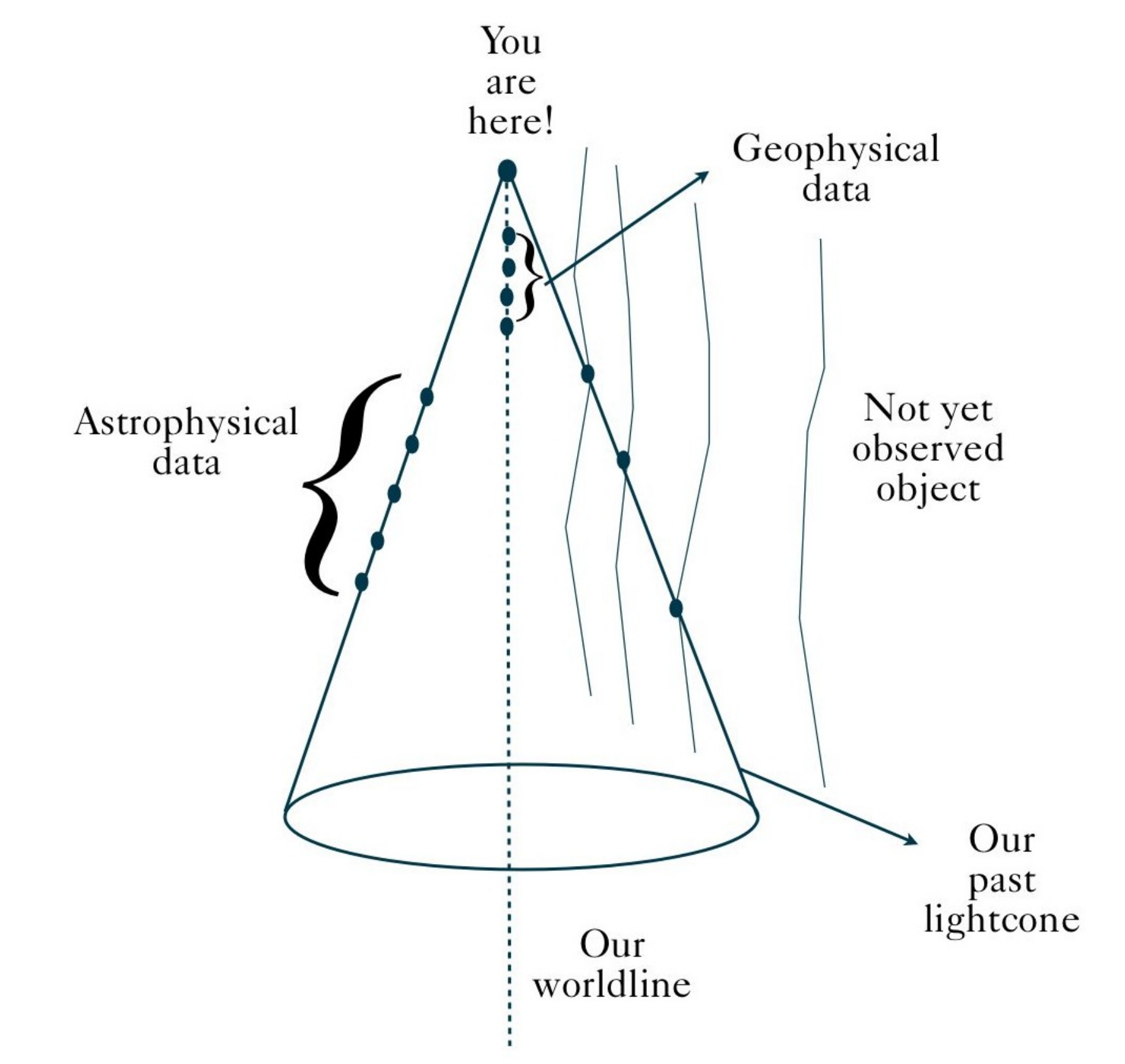
– For a given set of data, there are possibly many space-times corresponding to the observations. Again, as we have only one set of observations and since we cannot redo the experiment consisting in having the Universe evolving from the Big-Bang to now, we have no way to make sure our interpretation of the data is the correct one. We need to make some hypothesis on the nature of the structure of space-time and verify those. Only the large number of repetitions of observational data can reduce the risk of confusion between different models. Nowadays, we have so many data explained by one single model that it has become extremely difficult, if not altogether impossible, to come up with a different but equally successful model. One can already notice, at this point, that a further complication with any model of the Universe is that most of the hypothesis are hard to verify, since we can actually model our Universe, i.e. the observable one. The description of the actual Universe, which may even be infinite in size, does not belong to the realm of physics as we will never have access to it. Indeed, the Universe is probably much larger than the observable Universe over which we can collect data.
Let us now turn to what such a model consists of.
1.1 The FLRW model
The now-standard model of cosmology is called after Alexander Friedmann, Georges Lemaître, Howard Percy Robertson and Arthur Geoffrey Walker, who first introduced and discussed the corresponding metric and applied it to the Universe. The corresponding metric and space are called accordingly the FLRW metric, although for some unclear reason the ”L” is often omitted…
1.1.1 Theoretical hypothesis
The FLRW model is mostly based on 4 basic assumptions:
Theoretical prejudice and framework
Gravity is the leading force driving the dynamics, and we shall describe it by means of the General Relativity (GR) theory of gravitation. Based on the equivalence principle, it is an extremely well tested theory11 1 GR is accurate at the level of , i.e. it compares with QED as far as predictions are concerned. This constraint is obtained by measuring the orbital period variation of the binary pulsar system which implies emission of gravitational waves in exact agreement with GR. This measurements led to its discoverers, Russell A. Hulse and Joseph H. Taylor, sharing the Nobel prize for physics in 1993., in particular in the Solar System in which it serves as a reference for any alternative theory (scalar-tensor or MOND, for instance).
Gravity it is the only known unscreened long-range force, and thus appears to be very well suited to describe the largest scales and even the Universe as a whole. In assuming GR to hold on these scales, we suppose the locally derived laws of physics apply and can be extrapolated. On the other hand, if anything were to go wrong in our description, that would lead to a natural testing ground for GR.
The other interactions are assumed to be well described by the standard model of particle physics minimally coupled to gravity. This is achieved through the metric factor present in particular in the derivative terms: for instance, for a scalar field, the microscopic Lagrangian will contain a term of the form . Hence, the fundamental action we shall be interested in reads
| (4) |
It should be noticed again that any departure from this theoretical framework translates into observations different from the expectation, hence providing a way to test the validity of Eq. (4). In particular, scalar-tensor theories that would be equivalent to GR on Solar-System scales or for large cosmological times could originate (either in scale or time) very far from GR, and that could lead to observable consequences.
Reasons for doubting the validity of GR in astrophysics and cosmology include the flat rotation curves of galaxies and the currently observed acceleration of the Universe. At least at a phenomenological level however, they can be described by GR providing extra ”stuff” (dark matter and energy) is added to the matter content to which I now turn.
Matter content
Once the theoretical framework is fixed, one needs to set the matter content, i.e. the right hand side of Einstein equation (1). Observations, made only over luminous matter (and hence not precluding a priori any dark component) on the past light cone, reveal a single class of objects, the luminous ones! Therefore, we need to model not only those observed objects, but also any other component that we would not actually be able to see.
The typical distance scales involved are the galaxy characteristic size, of the order of light-years, and that of galaxy cluster, namely light-years. Hence, we do expect some amount of clumsiness on scales of these orders: the large scale structure of the Universe, being supposedly insensitive to the small scale effects, will then be defined on scales larger than light-years. On these scales, we will suppose the matter content to form a perfect fluid with normalized 4-velocity ( with a metric with signature -2) and stress energy tensor
| (5) |
where and are the energy density and pressure. The dynamics is usually imposed by setting , but this relates the time evolution of and in a contrived way: one needs to impose another relation, called the equation of state, expressing the pressure as a unique function of the energy density. In practice, a few simple cases are considered, always assuming a linear relationship, i.e. , with a constant called the equation of state parameter.
Observations reveal the typical relative velocity between galaxies (the point particles in the fluid element description) to be of the order in units of the speed of light. Therefore, the mean kinetic energy relative to the mass can be evaluated as , and this also provides a measure of the numerically expected value of the ratio between pressure and density: . Therefore, the fluid made up with the galaxies and any similar behaving fluid (dark matter) will be described by a pressureless gas, i.e. .
We also observed that the Universe is filled with some amount of radiation, whose stress energy tensor is traceless, thus implying . Finally, a cosmological constant term can be described by writing , and a direct comparison with (5) then shows that this implies , in other words . Amazingly, this extremely simple set of 3 constant equation of state fluids suffices to describe the evolution of the Universe for the previous 13.7 billions of years with percent accuracy!
Symmetries
Without symmetry assumptions, it is impossible to solve the full GR equations, even with a given (and simple) stress energy tensor such as that presented above, and so one needs to make even more simplifying assumptions, again based on observations. Those reveal the distribution of matter and radiation to be essentially the same in all directions. In other words, we see a space which appears isotropic. Figure 2 then implies at least two options following from these observations, of which the simplest is homogeneity (but spherical symmetry has also been studied), to which I will stick for now on. It should be emphasized that both homogeneity and isotropy are concepts whose validity in cosmology makes only statistical sense, and it is in this sense that they must be verified whenever possible.
At the level of Newton classical theory, homogeneity, stating that each point of space is similar to any other at each instant of time, is well defined. In GR however, the previous sentence is absolutely meaningless, and requires that a (space and time) slicing is done, hence generating a one parameter (time ) family of spacelike hypersurfaces . Homogeneity then is rephrased by saying that for any two points in , there exists an isometry taking one to the other. Isotropy on the other hand states that at each spacetime event, an observer moving with the cosmic fluid (comoving observer) cannot distinguish one direction of space from another one. One sees that the two notions are quite intricate, even though one describes a property of spatial hypersurfaces, while the other involves time development; this is due to the nature of our observations, always done along a light cone, hence mixing space and time measurements. Figure 3 clarifies these statements.
Assuming homogeneity and isotropy means that , restriction of the full metric to the hypersurface , only depends on time , so that is a 3 dimensional homogeneous and isotropic space with induced metric
as can be checked by direct calculation of a vector lying in or orthogonal to it.
Let be the Riemann tensor associated with the metric on . By its definition (2), it is symmetric in the exchange of the pairs of indices and and so can be seen as a map of the vector space of 2-forms onto itself: setting and , the matrix representing the 3 dimensional Riemann tensor is a symmetric matrix and thus diagonalizable. If its eigenvalues were not all equal, then one of them could be used to generate a privileged direction, in contradiction with the hypothesis of isotropy. Hence, we have , where can only depend on time, and the identity in the relevant space.
Moving back to 4 dimensional indices, we can write the 3 dimensional Riemann tensor in the form
| (6) |
Let us see the meaning of this expansion for to begin with, and embed the 3 dimensional space in a 4 dimensional Euclidian space with coordinates , and . A constant positive curvature space is a 3-sphere of radius whose point locations are given by
| (7) |
In spherical coordinates defined by
| (8) |
differentiation of Eq. (7) then provides the 3 dimensional metric in the form
| (9) |
where in the last line we have put back the possible time dependence of the overall spatially constant curvature.
Similar considerations with negative (3-hyperboloid) or flat (Euclidian) space permit to rewrite the overall 4 dimensional metric in the special FLRW (at last!) form
| (10) |
where the spacelike part of the metric is
where is the usual solid angle element and the function is to be continued for vanishing () or negative [ values of .
In the above relations, we have written to distinguish from the function giving the 3 dimensional Riemann tensor. In fact, it is always possible to renormalize the spatial coordinates in such a way that the scale factor has the dimension of length, so that can take one of the possible values . This is the choice we will assume for now on.
To finish this paragraph, I suggest to the reader to try and show, as an exercise, that the spatial metric can be cast in the equivalent forms
| (11) |
by means of changes of coordinates to be determined.
Topology
GR is a local theory which thus says nothing about the global structure of the Universe. String theory, of which GR is a low energy limit, teaches us that some dimensions may be compact, and in fact need be so in order for space to appear 3 dimensional on the scales available to experiments. Therefore, in principle at least, it is possible that the large dimensions we happen to live in could also be compact, leading to a non trivial topology. Although this has been studied in details, I shall not consider any further this hypothesis for at least two reasons, one experimental and the other theoretical.
First, there is no data, to date, that would induce us to think a large scale non trivial topology is needed. Of course, some compact models can be made compatible with the data, or even improve the fit, but they are degenerate with other models and the improvement is not really statistically significant.
Second, an argument in favor of compact large dimensions could be to invoke compactness for all dimensions; in this case, the expected phase of inflation would make the large dimensions much larger than the current Hubble scale (size of the observable universe), unless a disturbingly severe fine-tuning is applied. If a non inflationary scenario is implemented, then another fine-tuning is necessary in order to explain why the lattice size of the compact dimension should be, today, of the order of the Hubble scale (only case not yet ruled out by the data but still leading to observable predictions).
Having settled the framework, let me move on to the dynamics of our Universe.
1.2 The dynamical Universe
The framework developed above permits to write down explicitly the Einstein equations as a set of relations between a very small subset of dynamical quantities, namely the scale factor and the density of the fluid . In order to derive these equations, we need to calculate all the relevant geometrical quantities.
1.2.1 Geometrical quantities
The Einstein equations involve in a non trivial way the Riemann tensor and its byproducts, namely the Ricci tensor and scalar and the Einstein tensor itself. Those are all built from the metric connections and ultimately from the metric itself. It turns out that the cosmic time introduced earlier is not the most convenient time parameter, especially when the spatial sections are flat (which is observationally the case), and we usually introduce a dimensionless time, called the conformal time as it renders the metric conformally flat. It is related to the cosmic time by
| (12) |
where in the last stage we have taken the limit to make the Minkowski metric apparent.
To simplify matters, we define derivatives with respect to times as . Then, setting and , we obtain the only non vanishing connection coefficients as
| (13) |
in cosmic time, and
| (14) |
in conformal time. From these, one derives the non vanishing Ricci tensor components
| (15) |
leading to the Ricci scalar .
Combining these, we finally obtain the Einstein tensor as
| (16) |
This provides the left hand side of Einstein equations (1).
1.2.2 Friedmann equations and the cosmological parameters
With the geometric quantities derived for the FLRW metric, and the stress energy tensor (5) restated in matrix form as , it now remains to equal it to (16) to obtain the Friedmann equation, which the reader will straightforwardly check they can be cast in the form
| (17) |
for the constraint, and
| (18) |
for the dynamics. Deriving Eq. (17) with respect to time, taking into account Eq. (18) and reshuffling the various terms involved yields the fluid conservation equation
| (19) |
as expected since the latter conservation is not independent of the Einstein equations from which (17) and (18) stem.
In terms of conformal time, the previous set of equations read
| (20) |
for the conservation equation,
| (21) |
for the constraint, and finally
| (22) |
There exists a special solution, which happens to be realized in our Universe, at least so seem to say the data, namely that for which the spatial curvature vanishes. It defines a density, called the critical density given by
| (23) |
in terms of which one can express all densities in a dimensionless way. For each fluid component but the cosmological constant, one can set ; we also introduce an equivalent curvature ”density” as and finally , and then the Friedmann constraint simply reads:
| (24) |
so the Friedmann equation is understandable as an energy budget: all possible contributions basically sum up to 100%! Numerically, the Hubble constant today is measured to be of the order of , where . Similarly, the relative densities are also measured in units of the critical density, estimated as ; they frequently are found expressed as to account for the indeterminacy of the Hubble expansion rate as well as on the density parameter itself, the subscript “” meaning the present-day value.
1.3 Special solution: matter and radiation
With a varying equation of state and a scale factor , which is a monotonic function of time, it is always possible to parameterize all functions of time as functions of , and in particular . On can then formally integrate the conservation equation as
| (25) |
which gives an exact solution for the constant equation of state situation. This is precisely the case when matter () or radiation () dominates over everything else. Eq. (25) then shows that matter scales as , as expected from mass conservation in an expanding volume, while radiation gets an extra power, scaling as , due to the redshift of its wavelength. Now consider an initial condition consisting of given relative amounts of matter and radiation. When the Universe begins its evolution, with a small value of the scale factor, radiation dominates and the total density is until it gets caught up by the dustlike matter. This remarkably accurate picture for the Universe density evolution is illustrated in figure 4.
The meaning of the equation of state is clarified when one considers a perturbation propagating in the fluid. As is well known in fluid dynamics and as we shall also discuss later, the sound velocity is given22 2 In fact, it should be partial derivative for constant entropy. by . It can be shown (and the reader is encouraged to do so!), that the relation
| (26) |
holds, so that a constant equation of state means .
With the solution for the density as a function of the scale factor and the equation of state given, it is an easy matter to solve the Friedman equation. For a vanishing spatial curvature , one finds that if , the solution goes like
| (27) |
where I emphasized the particular pressureless dust and radiation dominated solutions. In the special case of a cosmological constant with , one finds
| (28) |
and one has an exponentially accelerated expansion; note in that case, which will later correspond to the inflationary situation, that the conformal time is negative, with the end of inflation being for the limit when .
1.4 Limitations of the standard model
The model developed above gives a quite accurate description of the history of the Universe, but its success actually raises a few questions that find no answer in its own framework.
1.4.1 Puzzles
Singularity
The first troubling issue is also the only one that has, in the inflationary paradigm, not received any answer, namely the fact that whatever solution of Einstein equations one comes up with that fits the available observational data does begin with a primordial singularity: at some point in the past, there is always a time at which , meaning all the geometrical tensors diverge, so the theory itself simply does not make sense anymore! One can however argue that GR is not designed to handle extremely high energies so that a cutoff, at the string or Planck scale, should be applied, above which the theory will (wishful thinking) be regular.
Horizon
The question of the horizon is more involved in a way, as no hand-waving argument can be similarly invoked to cure it. It relies on the observed fact that light emitted at decoupling (see figure 4) is homogeneous up to . Although this looks like a mere consequence of the cosmological principle, it is actually weird because of the previously discussed singularity problem: the existence of a primordial singularity implies a Big-Bang, i.e. a point in time at which the Universe expansion starts, so that there was a finite amount of time for a priori initially causally disconnected regions to thermalize. When one estimates the number of such regions, one finds some of those at decoupling, implying a predicted isotropy over angular scales smaller than roughly one degree on the sky only! Figure 5 illustrates the issue.
Flatness
Finally, the flatness problem is based on the fact that the observed flat spatial section (, i.e. ) is actually an unstable fixed point: in the absence of a dominating cosmological constant, deriving Eq. (24) with respect to the scale factor yields
| (29) |
whose solution, for a constant equation of state, reads
| (30) |
where . In order to observe now , one then needs to demand that at equality (), . which represents already a quite substantial amount of fine tuning if is to be an arbitrary initial condition. It becomes even worse of course if one assumes initial conditions ought to be imposed at one Planck time after the Big-Bang singularity itself, as the requirement then becomes : this is an unacceptably large amount of fine tuning!
1.4.2 Categories of solutions
There are nowadays two categories of solutions as far as I can tell, one widely accepted and usually set as part of the standard cosmological paradigm, namely inflation, and a contender based on a contracting phase and a bounce. Inflation does not address the singularity question, while a bounce is in danger of producing too much shear during the contraction. Moreover, inflation can be easily implemented using a simple scalar field, a de Sitter phase actually being an attractor in the equations of motion, while a bounce is almost impossible to implement in the framework of 4 dimensional GR unless the spatial curvature is positive. This makes inflation more appealing to most people.
Inflation
The Flatness problem originates from Eq. (29) and the fact that is an unstable fixed point for this equation. In fact, this is only true provided . If this condition is not fulfilled, as for instance is the case of a cosmological constant domination, then becomes instead an attractor. So it suffices to include a sufficiently long phase during which , then followed by the usual radiation and matter domination, to keep close to zero even after a long time of regular expansion. What is the meaning of this solution?
Equation (18) in the absence of a cosmological constant shows that if , i.e. if , then changes sign and the expansion is accelerated. This is why this solution was called inflation. Very often, it is implemented by means of a ”slowly rolling” scalar field, dubbed inflaton, i.e. a scalar field whose dynamics is dominated by the potential term, naturally leading to . As a result, inflation is achieved by an almost exponential growth of the scale factor.
Having a phase of accelerated expansion actually also solves without any further assumption the horizon problem. Indeed, the horizon size is a global quantity whose definition involves the overall history of the Universe through
| (31) |
where is the origin of times. Note that for a power-law expansion such as during most of the history of the Universe [see Eq. (27)], i.e. if , the horizon scales as , which is then roughly the same as the Hubble expansion rate . This, plus the fact that ”Hubble” and ”Horizon” begin with the same letter, has led to a confusion in many works between the two quantities. I will come back to that point later.
When an almost exponential phase of inflation takes place, the Hubble radius is roughly constant, while the scale factor grows exponentially. The horizon size is then
| (32) |
where the last inequality assumes . What happens then is that the horizon size grows much faster than the Hubble scale so that all scales end up having time to be in causal contact.
To be complete with the inflationary scenario, apart from its prediction of an almost scale-invariant spectrum of primordial fluctuations, I should like to mention that it is also the only known way of naturally reducing any initial amount of anisotropy. However, in order to reach an FLRW Universe, one also needs to impose a sufficiently smooth initial patch, i.e. even though inflation substantially alleviates the question of initial inhomogeneities, it does not actually answer it.
Bouncing scenarios
Eq. (29) can also be rewritten as
| (33) |
emphasizing once again that a phase of accelerated () expansion () will drive to vanishingly small values. Another way is possible, consisting in reverting all the signs of the previous argument, therefore using a decelerated () phase of contraction ()! Since we observe the current phase to be expanding, this implies that a transition between and took place, a bounce.
One might however argue that, as I said earlier, a positive spatial curvature is required to implement such a bounce in GR. One quick answer to this argument is that GR may not be valid at that time… after all, inflation also requires some extension of GR to account for the primordial singularity. Note in passing that the singularity is easily gotten rid of in the bouncing scenario since time can be pushed back as far as one wants, in principle even to infinity. This actually also solve the horizon problem, since it can easily be made infinite. To anyone not willing to extend GR in any way, one could also argue that it suffices to have a very long contraction phase during which , and manage that the bounce itself is not very asymmetric, so that even though can grow large during the bounce, it will recover a value after the bounce that is not very different from the one it had before.
The bouncing scenario however is plagued with an anisotropy problem: if one considers a initial shear, however tiny, it will grow very large during either the contracting phase or during the bounce itself. This is at least true in simple models, but more sophisticated scenarios have been proposed that tame these unwanted large growth.
Structure formation: perturbation theory
To obtain a complete description of the Universe, one would, at this point, need to include thermodynamical evolution of all the relevant quantities, taking into account interactions to describe in a reasonable way the phases of nucleosynthesis for instance. I shall not embark in this direction, and will instead concentrate on the perturbations over this background: those in fact provide a bonus for the inflationary scenario, as by demanding the inflaton to be in vacuum and allowing it to have quantum fluctuations, the ensuing evolution transforms the Universe in a particle producer, those particles then later behaving as large scale fluctuations seeding the formation of structures.
2 Perturbation theory: SVT and the gauge issue
It is widely believed that large scale structures formed out of primordial seeds upon which gravitational collapse acted to produce dense objects. This theory is quite well verified, as numerical simulations starting with an initial over-density function satisfying scale-invariant statistical properties manage to reproduce the statistical properties observed in large scale structure surveys. It lacks however a crucial ingredient: what is the seed origin?
2.1 Introductory remarks: the Jeans length
and Newtonian perturbation theory
Newtonian physics allows to understand the origin of gravitational collapse in the expanding Universe in a phenomenological way: one simply assumes that Newtonian gravity holds, but also that the Universe is expanding, i.e. that the actual distance between objects increases with time. One then has , where is the relative position of the object in a local coordinate system and the scale factor discussed in the previous section. The total velocity then consists in two pieces,
| (34) |
where the first term represents the background cosmic flow involving the Hubble rate , and the second the peculiar velocity, i.e. a relative velocity that one can treat as a perturbation.
Similarly, the density field is expanded as
| (35) |
and the continuity equation becomes
| (36) |
where the ‘’ term comes from changing the coordinate to . To zeroth order, Eq. (36) implies , which merely reflects that matter scales as , while the first order yields
| (37) |
where for now on we assume all spacelike derivatives are with respect to the ‘comoving’ coordinates ; I shall accordingly subsequently omit the index .
Combining Eq. (37) with
| (38) |
which is nothing but the Euler equation for a fluid with pressure in a gravitational potential (satisfying the Poisson equation ) in comoving coordinates, and linearizing, one finds
| (39) |
showing the Newtonian evolution involves three distinct effects, namely the damping of any perturbation due to the expansion, the propagation of sound waves due to the pressure terms, and finally gravity itself. In Eq. (39), the sound velocity is defined as before through where the fluid entropy is held constant.
Expanding in Fourier modes () and defining the physical wavenumber , one obtains, forgetting for the moment the expansion (i.e. setting )
| (40) |
where wavelengths are defined by , and is the celebrated Jean’s length separating regimes of wave propagation and gravitational instability: for long wavelength, , the density is growing exponentially with time, signaling a collapse, while for small wavelengths , the density oscillates as the sound wave propagates smoothly. Taking into account the overall expansion does not change this result qualitatively, it merely changes the functional dependence of the density with time, not the fact that there is a regime of unlimited growth and another of oscillations.
Having settled the stage, let me now move to the real issue, namely that of GR perturbations in FLRW Universe.
2.2 3+1 decomposition
For now on, I will mostly consider the conformal time , in terms of which the subsequent exposition is probably clearer. Then, the Friedmann (Einstein) equations are given by (21) and (22). Having completely fixed the background, we can now move on and expand around this background.
2.2.1 Perturbative expansion
Our starting point is the action (4) or, in practice, Einstein equations (1). As we did obtain the homogeneous and isotropic solution, we write it as , leading to the corresponding Einstein tensor , itself sourced by the background stress-energy tensor . We then write the full metric as
| (41) |
where the dots contain all higher order terms. We then assume that is a small parameter, as data indicate it to be the case on sufficiently large scales, i.e. on scales larger than roughly 200 Mpc. With Eq. (41) and the definition of the Einstein tensor, one can express it in the same way, namely
| (42) |
where is given by (16).
Similarly, we expand the stress-energy tensor (5) as
| (43) |
which amounts to expanding , and the fluid vector . Providing the series in powers of makes sense, it now suffices to expand both sides of Einstein equations and identify the terms, order by order.
In practice, there is no parameter, and we merely expand all relevant quantities as “background” + “something small” which we then calculate. The metric (denoting for now on the background quantities by an overbar) will read
| (44) |
whose “” limit would give (12) back. Note that the quantity should be the inverse of the above metric, so that demanding , we obtain .
The stress-energy tensor (5) has background values obtained with the choice , i.e. , and we also demand that the timelike vector be normalized at all orders, leading to , thus defining , and ; we see that it depends on the metric perturbation.
Gathering all terms for the stress-energy tensor, we finally obtain
| (45) |
where in the last term we have omitted a possible anisotropic stress contribution. The equation of state itself is perturbed assuming now that the pressure is a thermodynamical function of both the energy density and the entropy, if any: . The pressure perturbation then reads
| (46) |
where I indicate the most frequently used notations. The last one refers explicitly to the “non adiabatic” component of the pressure, which is proportional to the entropy variation .
2.2.2 Scalar, vectors and tensor components
In the perturbative expansion, we see appearing ordinary functions and indexed objects. The former transforms as scalars on the spatial hypersurfaces (recall we have an explicit 3+1 decomposition), while the latter transform as either vectors or rank-2 tensors of the spatial sections.
Making use of the covariant derivative associated with the metric , which we call , one can decompose all relevant quantities in terms of pure scalar, vector and tensor modes: for instance, the vector appearing in the metric (44) can always be written as
| (47) |
thus exhibiting a scalar function and two divergenceless vector degrees of freedom , recovering the three initial vector degrees of freedom. In a more common hydrodynamical framework for instance, that would be equivalent to splitting the velocity field into a velocity potential and a vorticity term .
The same technique applies to the tensor quantity which we write as33 3 We denote by round parenthesis the symmetrized part of the relevant tensor, i.e. .
| (48) |
where now the tensor is not only divergenceless but also traceless. This way, the 10 degrees of freedom of the metric are now split into four scalars (, , and ), 2 vectors ( and ) of 2 degrees of freedom each, and one tensor , also having 2 independent degrees of freedom. The main interest of this Scalar-Vector-Tensor (SVT) decomposition is that, at linear order, they all decouple, and one can thus treat the scalar, vector and tensor modes independently.
2.3 The gauge issue
GR is diffeomorphism invariant, i.e. it is constructed in such a way that general coordinate transformations leave the equations unchanged. This implies that out of the 10 degrees of freedom discussed above, 4 are essentially irrelevant as they can be absorbed into a coordinate transformation. When applied to the special background perturbations case, this invariance is no longer an actual coordinate transformations since the background is kept fixed; it is then called a gauge transformation. Let us see in more details how it works.
2.3.1 Metric fluctuations
Suppose I change the coordinates to a set of new coordinates related with the previous ones by an infinitesimal translation, i.e. , where are small quantities. General covariance then implies that the equations of motion have the same form when expressed in the “new” coordinates or the “old” ones . In particular, the line element, namely , should have the same structure under a gauge transformation. Therefore, we set
| (49) |
and by gauge invariance, we require that , after having SVT-decomposed the transformation through and . We find the following transformation laws:
| (50) |
for the scalar quantities,
| (51) |
for the vectors and finally . The last identity could have been obtained without any calculation from the vectorial nature of the transformation: tensor modes, also called gravitational waves, are naturally gauge invariant.
Equation (51) can easily be reshuffled into , so that the quantity is gauge invariant. On the scalar side, similarly, one finds that , so that , and finally that the quantity
| (52) |
is also gauge invariant. I leave it as an exercise to show that
| (53) |
closes the set of gauge-invariant variables consisting of two scalars and , called the Bardeen potentials, two vectors and two tensors for a total of 6 gauge-invariant quantities, as expected from the original 10 quantities and 4 possible gauge choices.
2.3.2 Choosing a gauge
One can play the same game with the stress-energy tensor and obtain transformation rules by expressing it in one frame or the other through the usual transformation rule of a rank-2 tensor. One finds
| (54) |
leading here also to a set of gauge-invariant variables
| (55) |
given here an only one example of such a combination.
From that point on, one can write down Einstein equations and solve them: just like in electromagnetism, one merely needs to fix a gauge. There are many gauges that have been used in the literature, and I list a few of them here. The first I want to list shows that the gauge-fixing choice is, just like in electromagnetism again, not necessarily enough: it is the so-called synchronous gauge, in which only spatial sections are perturbed. In other words, it is defined by assuming that the proper time of a comoving observer is cosmic time, and this translates into setting and . Because of its definition, it is a quite intuitive gauge, but it is not completely fixed: setting or for arbitrary fonctions and , one remains in this gauge ( and are still valid). This leads to possibly spurious solutions, and hence to mistakes!
Another frequently used gauge in the case of a single fluid is one which follows the fluid’s motion, so that one demands . This is an interesting choice which becomes unfortunately ambiguous as soon as more than one fluid is involved. In this gauge, the variables
| (56) |
are the natural fluid variables to use.
Another physically interesting choice is that which consists in demanding the curvature perturbation of spatial section to vanish, which amounts to setting and , so the quantities
| (57) |
reduce to their original values: these gauge-invariant variables are thus the density and pressure perturbations in the flat-slicing gauge.
Finally, it seems also appropriate to use directly a set of physically relevant variables like those defined above, namely the gauge-invariant ones. The simplest way to do that is to impose the so-called longitudinal, or Newtonian, gauge, i.e. that in which the scalar part of is diagonal so that we set . In this gauge, the potential (53) is the Newtonian potential. There are two possibilities to get to this gauge: one can either set from the outset (easy way) or work out all the equations and express all of them only in terms of the gauge-invariant variables (52) and (53). They both give the exact same results, of course. One sees that in this gauge, the density and pressure perturbations reduce naturally to those defined in (55).
2.3.3 Perturbed Einstein equations
We now are in a position to write down explicitly the Einstein equations to first order of perturbations in a meaningful way. The equations in the Newtonian gauge only involve gauge-invariant quantities, and I shall therefore restrict attention to those in what follows. Since the following section is dedicated to tensor modes, I will simply forget about them until then (remember they decouple at linear order anyway).
The next-to-simple case is that of vector modes. In most cosmologically relevant situations, there is no anisotropic stress (), so that the equations of motion of the vector modes are not sourced by anything. They take the form
| (58) |
and, more importantly
| (59) |
leading to the exact solution , and consequently, thanks to (58), that . It is a well-known (observational) fact that vector modes were negligible at the time of nucleosynthesis, so we may confidently set at . This implies now: apart in very special situations such as a contracting universe in a bouncing scenario, one can set the vector perturbation to zero. I shall not consider them anymore in what follows.
We are thus left with scalar modes. Since those have been driving the gravitational collapse leading to large-scale-structure formation, they are definitely the most relevant modes to study and, indeed, they play the first role in most of the literature on the subject. Their time development is obtained through two independent sets of equations, the first relating density to pressure perturbations, i.e. Eq. (46), the rest being given by Einstein equations, the spatial part of which, proportional to for a perfect fluid, yielding : under the reasonable assumption that the scalar perturbations do not diverge at spatial infinity, this relation implies that the only possibility is to have , a condition which I will take as valid for now on.
For the scalar modes in the longitudinal gauge, Einstein equations then read
| (60) | ||||
| (61) | ||||
| (62) |
Equation (60) can be reformulated as , using (56) and (61). This Poisson equation (up to the spatial curvature term) shows that the Bardeen potential is essentially the ordinary Newton potential if the density perturbation is expressed in the comoving gauge. As we shall see later, the matter perturbations in the different gauges on scales smaller than the Hubble radius are basically the same, so the sub-Hubble Bardeen potential indeed reduces to the Newtonian one (hence the notation ).
Now, using Eq. (46) to express the pressure perturbation in terms of the density, and then replacing (62) into (60), one obtains
| (63) |
which can be understood as the general relativistic version of Eq. (39).
Finally, this evolution equation can be made to a much simpler, intuitive and tractable form: by setting
| (64) |
one can check after a few tedious but straightforward calculation that Eq. (63) takes the wavelike form
| (65) |
where I have replaced the Laplacian in Fourier space. When there is no entropy perturbation (adiabatic perturbations), this equation is simply that of a parametric oscillator; the entropy contribution can then be seen as a forcing term. As it turns out to be the same as the gravitational wave case, I now move to those.
3 The example of tensor modes
Tensor modes, being gauge-invariant from the outset, are free of all gauge-fixing subtleties, and can be computed straightforwardly. Einstein equations for those read
| (66) |
where the anisotropic stress is usually set to zero, in agreement with the observations. Moreover, as we have seen, the spatial section curvature is also measured to be quite small, so we can safely set it to zero as well. Since inflation also set both these quantities to vanishingly (exponentially) small values, we have both observational and theoretical good reasons to set and .
3.1 Flat space polarization
In order to understand what a tensor mode is, it is simpler to first consider the non expanding case in which we set , so the Einstein equation for reduces to the wave equation
| (67) |
whose solutions I now discuss.
3.1.1 Polarization.
Let us consider for simplicity a mode propagating along the direction, and pick the simplest possible solution of (67), i.e. . Now what is missing in this solution is the set of indices, which account for the polarizations. With , the transverse and traceless conditions for read , and . We are thus left with two independent solution, and say. These are the functions behaving as sines and cosines.

The full solution can be expressed in terms of these functions together with a set of polarization tensors and , namely
| (68) |
whose names stem from their effect on a test particle.
3.1.2 Observing a gravitational wave
Let us consider two such neighboring test particles following their own paths and (see Fig. 6) and assume they are originally at rest. The connections being vanishing at first order in perturbations (only is present), as the wave passes, a particle originally at rest remains apparently so: the particle is moving with the reference frame. However, the perturbed curvature is non vanishing, so the relative geodesic motion is affected by the wave. The geodesic deviation between these geodesics feels an acceleration given by
| (69) |
so that the distance between the ring-forming particles changes with time as
leading to the time evolutions shown in Fig. 6.
The very simple cosine and sine solutions are obtained in the flat Minkowski case, and can readily be generalized to the expanding case with a scale factor increasing as a power law: they are then replaced by Bessel functions, see below.
3.2 Cosmological gravitational waves

Even under the simplifying assumptions made below Eq. (66), one still needs take into account the tensorial nature of the modes. Because this equation is linear, it can easily be decomposed into Fourier modes in the form
| (70) |
where is a polarization index (running from 1 to 2 because of the two degrees of freedom in the tensor modes), and the polarization tensor can be given explicitly as follows. Note the factor which has been put here for further convenience.
3.2.1 Polarization modes
Figure 7 displays the configuration for the wave vector and the orthogonal plane in which one defines a dyad () satisfying and . Recall that the tensor mode is transverse and traceless, which translates into the polarization tensor as the requirement
| (71) |
(we have set and thus can identify ). One can check that the choice
| (72) |
satisfies all the constraints (71).
Plugging the form (72) into Eq. (66) then shows that both quantities satisfy the same differential equation. We then simply set (the index ‘T’ standing for tensor, we will later have a similar variable with an index ‘S’ for the scalar case) and obtain
| (73) |
which is the prototypical wavelike equation obtained in cosmological perturbation theory. It is interesting to realize that it can be obtained by varying the Einstein-Hilbert action expanded to second order in perturbation, namely (for the general case including curvature)
| (74) |
in which one recognizes the action of a time varying mass scalar field. This observation lies at the heart of the idea of setting quantum initial conditions, as I will explain later.
3.2.2 Time development of a mode
Let us go back to the original equation (66) in the case of an expanding Universe dominated by a perfect fluid with constant equation of state. In this case, we have seen that the scale factor behaves as for some value of , and the Hubble function then takes the simple form . Eq. (66) thus becomes
| (75) |
where . As announced earlier, this is a Bessel equation whose solutions have been studied in details since the beginning of the 19th century. They are shown on Fig. 8 and read
| (76) |
where the tensors and are, of course, transverse and traceless.

The solutions show two extreme regimes, called sub- and super-Hubble. They refer to the characteristic ratio of the wavelength () to the Hubble scale ( for a power-law scale factor), i.e. the variable . Long wavelengths () are strongly damped by the expansion, and so any initial motion is rapidly erased by the expansion-induced friction and the mode behaves as a constant. For short wavelengths () on the other hand, the expansion is negligible and the mode behaves essentially as in a Minkowski universe: we recover the oscillations obtained earlier.
3.2.3 Hubble vs Horizon
At this stage, I think it is important to make a short comment on a commonly used and very misleading phrase, namely the use of “sub-horizon” and “super-horizon” modes instead of sub-Hubble and super-Hubble. As shown by Eq. (31), the horizon is a global quantity which depends on the entire history of the Universe. Early models were based on the singular big-bang followed by radiation and matter dominations, and it is easy to convince oneself that in this case, the integrated quantity is, up to an irrelevant numerical factor, given by the Hubble scale. In such a context, comparing wavelengths with the Hubble radius would indeed be equivalent to comparing them to the size of the horizon… but it is then not very clear what the meaning of these would have been! Indeed, in GR, modes larger than the horizon are actually not well-defined in the sense that setting initial conditions for them would be a direct violation of causality.
In fact, one often reads that the modes are ‘‘frozen’’ because of some ‘‘causality’’ reason, with the meaning that a mode larger than the horizon could not evolve at all because of causality, as both ends of the mode would need to propagate faster than light to communicate, which is forbidden. I do not know what is the meaning of such arguments, and strongly suspect they have none whatsoever. A given mode consists of a linear combination of the two independent functions solving a second order linear equation44 4 This discussion is also valid in the case of scalar perturbations, so I do not restrict attention here to the tensor case., with coefficients provided by the initial conditions. Then, for a super-Hubble wavelength, what happens is that the expansion very rapidly suppresses one of the solution relative to the other, and one is left with the constant mode as discussed above. But this is in no way related with causality, on the contrary, it is a purely dynamical statement.
We have discussed this point in more details in Ref. Martin and Peter (2004) for the specific case of scalar perturbations in bouncing models.
3.2.4 Radiation-to-matter transition
With the mode evolution known in any given epoch and a primordial spectrum, one should in principle be able to predict the observed spectrum. As it turns out, the theories that agree with the data predict an almost scale-invariant initial spectrum, i.e. one in which no particular scale is singled out. On the other hand, we know that such a scale should be present somehow, because the Universe, which was at very early times dominated by radiation, transitioned to the matter era55 5 There was another transition more recently when the Universe became dominated by the cosmological constant or whatever it is which mimics it nowadays; I will not discuss this any further, but in principle, it could well lead to another scale in the data indeed..
The transition can be treated simply by introducing a new variable , where is the value of the scale factor at equality between radiation and matter, shown in Fig. 4 and defined through . Given that and , we find that , and finally that . I leave as an exercise to the reader to show that the total equation of state , defined as the ratio of the total pressure by the total energy density, is and the sound velocity is .
The Friedmann equation (21) takes the form
| (77) |
thus allowing to switch to the variable whenever one encounters . Noting that the derivatives with respect to and satisfy
and defining the wavenumber characteristic of equality as , we find that Eq. (66) takes the following form
| (78) |
whose analytic solution is not known… but we can solve it numerically for different values of . This is done in Fig. 9.

Let me conclude this section by returning to the form (73) of the mode equation. Its formal solution is known and given by the Born expansion, namely
| (79) |
i.e., we have replaced a differential equation by an integral one! However, we have gained something in the process because the solution is known exactly in the long and short wavelength limits. They are, for short scales
| (80) |
and for the large scales
| (81) |
so that it suffices to plug one of these solution into (79) to obtain an expansion in either large or short wavenumbers.
One final point, regarding the action (74) and the solution (80) valid for small wavelengths, i.e. when the expansion can be discarded: in this case, we can consider as an actual scalar field in a Minkowski universe, a system which we know how to quantize. Once the field itself is quantized, one can impose a given physical quantum state, for instance the vacuum. But this actually fixes unambiguously the coefficients and … and then, the theory becomes predictive! I shall return to this in the last part of these lectures.
After having discussed the tensor modes in quite some depth, let me now sketch the scalar case which, although currently the only one observed, is also sufficiently more involved to require a special treatment of its own. This is done in Refs. Peter and Uzan (2013) and Mukhanov (2005).
4 Density fluctuations and the power spectrum
Since the tensor modes have not been observed yet, let us move on to the scalar case. For this, I will set a much oversimplified (and already disproved by the data!) model having , i.e. , and assume all there is to consist of matter now (i.e. ) with a currently negligible amount of radiation .
4.1 Basic equations
Before we move on to our specific example involving basically only matter () and radiation (), let us write down the more general set of equations for a fluid having constituents, e.g. radiation, dust, neutrinos, dark energy, dark matter, and whatever else a theoretician’s brain can come up with.
The total energy density and pressure allow to define a global velocity through . The total equation of state and sound velocity can be obtained as
| (82) |
where each fluid sound speed is .
Similar calculations can be made at the perturbation level, yielding for the density fluctuations and for the velocities. The total entropy perturbation can be derived in much the same way as for the single fluid case, namely recalling that we set , we get , and finally
| (83) |
showing that even if each individual fluid has vanishing self entropy perturbation (i.e. even if all ), the total fluid mixing entropy can be non vanishing.
In principle, if the fluids are coupled, one should not necessarily assume them to be each independently conserved, but rather to satisfy (the condition in parenthesis being redundant)
| (84) |
assuming some action/reaction principle for the various fluid components. For the background, setting , we have the generalization of (20) to a many-component fluid, namely
| (85) |
In practice however, since we shall here restrict attention to matter and radiation, we set the forces acting on the fluids .
In terms of these variables, the relevant Einstein equation reads
| (86) |
showing how to relate the large-scale structure distribution (the density fluctuations) to the metric perturbations. The perturbed densities and velocities, when both the forces and the self entropies are vanishing, follow the continuity and Euler equations
| (87) |
Let us specialize for now on to the case of two fluids. Introducing the gauge-invariant relative velocity and entropy perturbations
| (88) |
relation which can be inverted through
| (89) |
the continuity equation can easily be restated as
| (90) |
while Euler equation reads
| (91) |
The basic idea now consists in solving Eqs. (90) and (91) together with (63) so as to get a complete solution for the distribution of now through (86): this density perturbation spectrum can then be directly observed as the large-scale structure distribution. This is more easily said than done, and to begin with, one needs to impose initial conditions, to which I now turn.
4.2 Adiabatic and isocurvature initial conditions
In order to impose a complete set of initial conditions, we need to know the number of independent degrees of freedom. As soon as one knows all the fluid variables, the system is fixed, namely knowledge of all the and is enough. For the two constituent fluid we are dealing with, this means we need 4 independent conditions. With the previous variables, we can re-express all these in terms of the sums and , so that then Eqs. (86) and (61) provide and respectively. We are then left with the relative velocity and entropy perturbations and .
There are basically two sets of initial conditions which are used, the so-called adiabatic and isocurvatures ones. They are defined by the following conditions.
- •
Adiabatic initial conditions: the entropy perturbation (88) vanishes at the initial time, while the Bardeen gravitational potential is a constant, so we have
(92) leaving two arbitrary initial numbers, and say, to decide of the forthcoming mode evolution.
- •
Isocurvature initial conditions: the opposite, and complementary, situation consists in setting initial conditions such that there is no initial metric perturbation, i.e. we set at the initial time
(93) which, again, leaves 2 arbitrary numbers to be set, for instance the values of and the initial entropy .
These conditions essentially reflects all the possibilities, and the “real” initial perturbation should be a linear superposition of those.
It should be reminded at this stage that these initial conditions ought to be set at the point in time after which we can evolve them with sufficiently precise knowledge of the cosmic history. Normally, this is done using a simulation code taking into account all known relevant cosmological phenomena. This means we assume that the initial spectrum of perturbations is propagated through the almost entire history of the Universe from this original time… the question then remains of what is this initial time, and how can we even suppose we know anything at all about it? That will be the subject of the final section, but for now on, let us concentrate to the actual evolution and the spectrum we might get now so as to be able to compare with observational data!
4.3 Mode history
As discussed above, we now specifically restrict attention to a flat, matter-dominated Universe containing a tiny amount of radiation, so that Eqs. (87) now read, in Fourier space,
| (94) | ||||
| (95) |
and we assume we know, somehow, the initial conditions for the perturbations deep into the radiation epoch. Adding the Fourier-transformed Poisson equation
| (96) |
closes the system which we now solve.
4.3.1 Initial conditions in the early radiation epoch
The Universe will have to go through the radiation-to-matter transition, and we thus switch to the relevant time variable defined above Eq. (77) and in terms of which the relative density parameters read
Since now and noting the relationship between the comoving total density perturbation and the Bardeen potential
we see that the entire system reduces to the set
| (97) |
Once we have the solution to the system (97), we can reconstruct the density perturbations through
| (98) |
We now want to impose initial condition very early on, when the Universe is radiation dominated, i.e. for , and we are interested in cosmologically relevant wavelengths, i.e. those satisfying . If we decide for adiabatic initial conditions, this means we can demand
| (99) |
turning Eq. (98) into
| (100) |
leading to
| (101) |
These initial conditions mean that the density ratios are constant everywhere on the initial hypersurface: both density perturbations behave in the same way everywhere, as illustrated in the left panel of Fig. 10.
Setting isocurvature initial conditions on the other hand amounts, in this case, to imposing at the initial time the relations
| (102) |
which translates, in terms of density perturbations, into
| (103) |
with all velocities vanishing. This is also illustrated in Fig. 10, on the right panel.
4.3.2 Transfer function
Let me now move on to the transfer function, which is defined as the ratio of the observed spectrum of perturbations now, i.e. essentially the large scale structure distribution in the sky, with the primordial spectrum, as calculated by high energy physics; this primordial spectrum is the topic of the final section.
Let us consider a given mode, i.e. a given wavelength , and solve the equations of evolution (97). Without entering unnecessary details that can be found elsewhere Peter and Uzan (2013); Mukhanov (2005), suffice it to say that the main behavior of the perturbations depend on two quantities, namely the time at which they are evaluated relative to the equality time , and the comoving wavenumber of the perturbation, again relative to the value , defined above Eq. (78). Fig. 11 shows the various possibilities by comparing the wavelength with the Hubble factor entering the evolution equations.

One finds the following time developments:
- •
- –
: ,
- –
: ,
- –
: .
- –
- •
- –
: ,
- –
: ,
- –
: .
- –
We see that for most of the time, the density perturbation in the matter fluid evolves as the square of the conformal time, except for the modes whose wavelength is smaller than the equality scale: those become sub Hubble during the radiation dominated phase, during which they cannot grow because of the photon pressure. This is shown in Fig. 12.

The previous time evolution transforms into a change in the spectrum for scales above . Indeed, a mode with evolves essentially as all along, so that , with the index “0” still denoting the present-day time. Similarly, a mode with evolves as only up until , at which point it behaves roughly as a constant. As a result, when it starts growing again, at , its value is . The transfer function is now defined as the ratio between the final (evaluated at ) and initial (at ) density perturbations, namely
| (104) |
and the calculation above shows that for (long wavelengths) and for (short wavelengths). The insert of Fig. 12 also shows the typical behavior of the transfert function.
4.3.3 Perturbation spectrum
With the transfer function known, we can now derive the actual large scale structure distribution, can we? Well, in fact not quite yet, as there is something missing: the initial distribution . This will be the subject of the last section, as I already mentioned a few times, but something can already be said at this stage, in particular by looking at the data.
The only analysis that can be done of all the observation is statistical in nature, as we now understand the actual density distribution to be but a particular realization of a statistical ensemble, so that the density field itself is now seen as a random variable at each point. What is actually measured then is the correlation function of the density field, defined by
| (105) |
where the mean value should represent an ensemble average. In practice however, we have only access to one such realization, and we replace the ensemble average by a spatial average. Note at this stage that the cosmological principle implies that the distributions should be isotropic and homogeneous. As a result, the correlation function should only depend on the distance scale and neither on the particular direction choice nor on the specific point .
Moving to the Fourier space, we can write
| (106) |
whose spectrum stems from the two-point function in Fourier space, namely
| (107) |
I leave as an exercise to show that it is the Fourier transform of the correlation function, i.e.
| (108) |
and, as expected again from the cosmological principle, it also does not depend on the direction but merely on the wavenumber .
In a way, the power spectrum can roughly be seen as the square of the density distribution. Therefore, we also have the relation
| (109) |
which is the equivalent of (104) for the spectra.
We shall see later that the expected primordial spectrum actually scales like , and so the observed distribution should scale as for long wavelengths where the transfer function is independent of scale, and as for shorter wavelengths. Fig. 13 roughly confirms these expectations.

A quick estimate of the equality scale is provided by
which is estimated to a hundred Mpc, falling a bit short of the actual value. This is due to our very rough approximation according to which our universe model only contains matter and radiation.
The actual transfer function is in fact much more complicated to calculate once one takes into account all the cosmological constituents. For instance, if there is a so-called hot dark matter component, consisting in relativistic degrees of freedom at the time of decoupling, e.g. neutrinos, it has the effect of streaming easily throughout any initial perturbation, thus wiping out very large scales. These scales cannot grow anymore, and this produces an exponential cutoff in the transfer function.
5 Initial conditions: quantum vacuum fluctuations
So far, this presentation contained essentially no new physics, merely basic applications of general relativity and fluid dynamics. It can all be made much more precise, e.g. to include thermodynamics and using the Boltzmann equation, but this would also be well-known physics and in no way can ever provide what we are seeking, namely the initial conditions for the perturbations we have just calculated. In fact, measuring the large scale structure distribution while knowing all what precedes is akin to measuring the initial conditions, which is kind of useless if we don’t have a theory that predicts them.
It turns out that soon after the advent of inflation, which was originally the first convincing scenario that was proposed to cure the puzzles discussed in the first section of these lectures, it was realized that the accelerating epoch had the ability not only to enhance already-existing perturbations, but also to produce those when quantum vacuum fluctuations were taken into account. Since that time, other models, for instance including an initial contracting phase and a bounce to connect to our currently expanding epoch, have been devised that also provide the required initial conditions, and they can be tested quite accurately with the more and more precise data that are accumulating.
Although the inflationary paradigm is the best accepted one to describe the primordial epoch, I would like first to emphasize that it is not established beyond any doubt (as one sometimes reads!), so that looking for challengers is still a reasonable activity. However, in what follows, I will restrict attention to the inflationary case as it is easier to implement and pedagogically more convenient.
5.1 Back to the background
Inflation provides explanations to the standard model puzzles by means of acceleration of the scale factor, namely for a finite but sufficiently long period of time, we have . Eq. (18) then implies that the pressure should be more negative than a third of the energy density (which is always assumed positive). This is easily achieved by means of a slowly-rolling scalar field whose action we take to be
| (110) |
with a yet-undefined potential .
5.1.1 Slow-roll parameters
The stress-energy tensor derivable from the action (110) is
| (111) |
where the definition of the energy density and pressure assume the field to depend only on time in order to satisfy the background symmetries. We see that the r.h.s. of Eq. (18) reads , which can be negative quite easily provided the kinetic term is sufficiently small compared with the potential. Because then the velocity of the field is tiny, this is why we speak of slow-roll phase.
The Einstein and Klein-Gordon equations then transform into
| (112) |
where the last of these, merely reflecting the conservation of (111), is not independent of the first two. Combining those actually yields : as is assumed small, the natural tendency for is to decrease as the scale factor increases. But this makes the scale factor increase even more rapidly, so the spatial curvature term becomes more and more negligible. In fact, this is an attractor of this system of equations, and therefore, for now on, we will assume with the meaning that spatial curvature terms are exponentially smaller than any other.
Applying the slow-roll conditions and , we find the relations
| (113) |
which are consistent with the original assumptions only if . More generally, one can define two small parameters, called the slow-roll parameters, by
| (114) |
Inflation goes on for as long as , which translates into .
The simplest solution for this model consists in demanding to be constant; in this case, the scale factor can be calculated as follows. First, I recall the relationship between conformal and cosmic time, namely
| (115) |
so that, noting we also have
| (116) |
this means that the relation
should hold, and if is roughly constant, we can perform the integration, leading to
which I can invert and obtain that the scale factor behaves as
| (117) |
i.e. we have an exponential quasi de Sitter phase. The parameters and are constant of integration necessary to pass from conformal to cosmic time. Eq. (117) shows moreover that inflation occurs in the regime where and .
5.1.2 Two explicit examples
The simplest example one can think of is that for which the scalar field is merely a massive free (non interacting) field, namely the potential reads . In this case, the system (113) reads
| (118) |
where use has been made of
The scale factor is then
from which one obtain the slow-roll parameters as
| (119) |
As varies with time, we can easily calculate when the slow-roll phase ends, namely for , so the number of e-folds of inflation is . In order to solve the cosmological puzzles, we know that we must impose , leading to the requirement that the initial value of the scalar field should be of order . One might think that this could be a problem, as such a high energy scale would require quantum gravity to be described properly, and of course we do not have such a theory. However, what actually matters is not the field value itself, but the energy density that it stores. Under the slow-roll hypothesis, this means the potential energy, i.e. provided the scalar field mass is much less than the Planck scale. As we shall see below, this is exactly what is required from the data.
Another useful model is the so-called power-law inflation, for which one demands the scale factor to increase as a power-law instead of an exponential, while still being accelerated. Explicitly, this is
| (120) |
where and are constants, and to ensure that .
Integrating (113) equations again, one obtains the scalar field behavior
and the potential it evolves in
together with the slow-roll parameters: . Since there is no time evolution in this case, we see that such a model has merely a pedagogical value, as inflation never ends in this case. However, it can really be useful because many features are calculable in an analytic way.
Having settled and somehow implemented the inflationary phase, let us see what happens to fields living in such a background.
5.2 A test field in inflationary background
We shall here follow the evolution of the simplest case, namely that of a test field in an inflationary background which, to make things even simpler, we shall assume takes the form of a quasi de Sitter expansion, i.e. an actually exponential expansion, or Eq. (117).
5.2.1 Massless scalar field
Let us begin with yet another simplifying assumption, namely that the test scalar field is massless, so its potential vanishes. The Klein-Gordon in the expanding background reads
| (121) |
where in the last equality I switched to the conformal time and took the Fourier transform. Now, setting , thereby defining , we find that
| (122) |
where I have used Eq. (117).
Eq. (122) is the same as that driving the evolution of the tensor modes (73), and is of the generic form of a ”time-independent” Schrödinger equation in a potential (regarding the conformal time variable as the equivalent of the spatial coordinate):
| (123) |
provided one identifies with , with and rescale everything to cancel out the . In fact, whenever there is no entropy perturbation, it is the most generic form we will ever encounter. So for now on, I will assume a generic potential , and discuss the actual mode evolution.
5.2.2 Evolution regimes
The potential during inflation grows like when , but this is merely an artifact of our approximation. In a realistic scenario however, the potential might look like that represented in Fig. 14: it starts growing during the phase of inflation (or in general any such phase during which primordial perturbations are produced), and reaches a maximum, after which it decays. These last phases would usually represent radiation or matter domination, at which times we would observe the mode somehow: the scale factor would then behave as , so the typical potential should look like .

Figure 14 summarizes the discussion of the tensor modes, with the same kind of solutions (80) and (81); I shall not repeat this analysis here, but suffice it to say that it also applies to most known cases as very often the potential has the form of the second time derivative of a function over this function.
In the special case of de Sitter expansion, i.e. (117) with , the solution is known, since this is then a quite simple Bessel equation, and we have
| (124) |
where and are yet-unknown function depending only on the scale .
The massive scalar field case can be obtained in a very similar way as it suffices to replace (123) by
whose solution is again another linear superposition of Bessel functions of index , with .
5.3 Quantization
All what precedes does still not tell us what initial conditions we should use, or, in other words, given (124), what should we take as functions and ?
To achieve this goal, we need to quantize our system, which is quite simply done when we have discussed the action expanded to second order.
5.3.1 Expanding the action
The action for our scalar field, still without a potential to keep things simple, is
| (125) |
which we can express in terms of the variable as
showing it is nothing but the action for a simple scalar field in Minkowski space… usual technique of quantum field theory can now be applied, and we will have the possibility of choosing a specific quantum state to provide the initial conditions.
5.3.2 Canonical quantization
We can expand the field as any standard quantum field through
| (126) |
the second term being the hermitian conjugate of the first.
Quantization is achieved by promoting to an operator in the Fock space of field configurations and imposing the canonical commutation relations
| (127) |
These relations can be seen as stemming from the actual field quantization: defining the conjugate momentum
with the Lagrangian being the integrand in the definition of the action, the Hamiltonian follows
and we can impose the standard equal time commutation relations for the field operators, namely
| (128) |
These commutation rules are consistent with those above (127) only provided the Wronskian is normalized to since one gets directly from the field expansion
We are almost done, having merely to define the relevant state to assume as initial condition.
5.3.3 The vacuum state
In quantum field theory and therefore here as well, the vacuum state is that which is annihilated by all the so-called “creation” operators , namely
and all other states are obtained by repeated application of the operators on .
In the limit , i.e. for large negative conformal times where we indeed want to impose our initial conditions, we are back to the usual massless scalar field in a Minkowski space time, and we know that the vacuum state must therefore satisfy
as indicated in any standard textbook on quantum field theory. Given the previously obtained solution, this leads to the so-called Bunch-Davies vacuum state
| (129) |
which now provides a closed form initial solution for our perturbation. It is with such initial condition that one finally gets the scale-invariant spectrum which one compares with the observational data (and it works!).
The power spectrum is now obtained from the 2-point correlation function , which gives
| (130) |
after integration over the angles and setting .
It turns out that for large scales, i.e. super-Hubble modes, one finds that the properties of a quantum field are the same as that of a classical stochastic field with gaussian statistics. In particular, this means we can replace the quantum averages by statistical ensemble averages. For the stochastic variables, we find a power spectrum that scales as
| (131) |
in other words a scale-invariant spectrum.
5.4 Realistic perturbations
If one wants to take into account all the actual complication of what is really going on, one needs to consider all scalar, vector and tensor modes of the metric and treat them including all possible effects. Although this is a very complicated task, some situations allow to say something however. For instance, assuming the scalar field to drive the early history of the Universe, one finds that the gauge-invariant degree of freedom generated by the variable
| (132) |
thus defining the so-called Mukhanov-Sasaki variable , is enough to describe all the fluctuations in a single field inflation. Expanding the action to second order in perturbation and getting rid of the surface terms just as above, one arrives at
| (133) |
thus showing what I previously said, that the typical equation of motion is always of the same form. As the same analysis applies, one thus obtains a way to set up initial conditions by assuming quantum vacuum in the early stage of the Universe. This leads to a natural way to obtaining a scale-invariant spectrum that fits extremely well all the known data.
6 Conclusion: Conditions for alternative scenarios, the bouncing model
The cosmological scenario, as discussed in the notes above, represents a major achievement in physics, performed in less than 100 years! In that time, it has been established that the Universe itself could be treated, studied and understood as a regular physical system, despite the fact that it seems to contradict, by its very uniqueness, the usual assumptions of the scientific method. In fact, cosmology somehow extended the inductive method, replacing for instance repetition of experiments by repetition of measurements in different directions, in other words, replacing ensemble averages by ergodicity.
To summarize, we now have a rather clear view, basically, of what happened during the last 13.7 billion years, with detailed calculations comparing amazingly well with observations. Although I did not discuss them all, but these observations range from consequences stemming directly from nuclear physics (nucleosynthesis), thermodynamics, fluids mechanics, gravitational phenomena, and, as sketched in the last section above, the relationship between gravity and quantum physics! That only a bunch of ”unpleasant” features are present in the data with the overall picture being generally consistent is absolutely astounding and very often not given enough emphasis.
Now our cosmological model, precisely because of its successes, can be scrutinized with exquisite attention to unveil any possible new mechanism the we would not have thought about. This is how detailed examination of specific objects (Type Ia SuperNovæ) and their redshift distribution revealed that the Universe appears to be currently accelerating (see however D. Wiltshire’s contribution in this volume for an alternative understanding of the data), leading to a new component, dubbed dark energy, among the various fluids pervading the Universe. When added to the other components, it permits to fit all available data, including large scale structure distribution, SuperNovæ or the Cosmic Microwave Background (CMB) fluctuations (see Fig. 15).

Figure taken from Hinshaw et al. (2012) in which all references to other data are provided.
There are many things lacking in this presentation, including not only the CMB fluctuations themselves, but also its polarization and measurement thereof, non gaussianities, baryonic acoustic oscillations, and many others. One special point I would like to emphasize over however is that when all those data are taken into account, the whole thing can serve not only to check the currently accepted paradigms and models (an inflationary phase followed by radiation, matter and cosmological constant dominations, the so-called CDM model66 6 Meaning for the cosmological constant, and ”Cold Dark Matter”, this phenomenological model describes with the minimal possible number of parameters the current data.), but also to explore alternative possibilities: although the inflationary paradigms seems to provide satisfactory explanations to most of the cosmological puzzles, it is not still proven beyond reasonable doubt, and besides, it has a few problems of its own.
Inflation is based on well under control physics, i.e. GR and quantum/classical scalar fields, it can be implemented in high energy theories such as Grand Unification or string theories, and it makes predictions which have been experimentally shown to be compatible with observations… why would we therefore like to find any alternative at all? First of all, it does not really solve all the puzzles, as in particular, the question of homogeneity, although admittedly alleviated, is by no means solved. Moreover, an inflationary phase usually begins from a singularity, or from a quantum gravity fluctuating phase, which is not understood at all. Related to this is the fact that even the largest possible scales observed today, i.e. that of the Hubble radius, must have inflated and expanded from a time where it was actually smaller than the Planck length itself. Setting initial conditions there is, to say the least, debatable. Finally, providing challengers is always a very good way to test a theory, so inflation itself benefits from alternative models.
Most alternative to inflation present, in one way or another, a contracting phase preceding the currently expanding one, to which it is related by means of a bounce. This is not a new idea, as it was in fact suggested in the 1930’s by Tolman and Lemaître, i.e. much before any inflationary scenario was even thought about. In course of time, bouncing scenarios were repeatedly proposed, as discussed in Ref. Novello and Bergliaffa (2008). One might immediately argue that this seems to create more problems than it solves, since in particular it is very difficult to implement a bouncing phase in the framework of GR; however, the bouncing model also addresses different issues. For instance, there is of course no question of the primordial singularity, which is avoided by definition! Moreover, the horizon (31) can easily be made infinite if the initial time is sufficiently large and negative, i.e. in the limit . Flatness is also quite a natural achievement of the bounce, as I discussed earlier.
Now perturbation theory ought to be valid as well in a contracting background, so basically, all I said before applies straightforwardly in such a new framework. What needs be done then is to evolve similarly set vacuum initial conditions in the contracting Universe all the way to the bounce and up to now. In general, what happens is the following: whenever the relevant equation of the perturbations takes the form (123), the potential can be more complicated than that shown in Fig. 14, and in particular it often happens that the term changes sign more than once or twice. As a result, the primordial spectrum starts oscillating before it gets amplified again, and one expects oscillations on top of the usual and expected oscillations. For the time being, no observation has been made along these lines, but one can hope to see those in the future, e.g. with Planck data.
Finally, I should say that the perturbation question is somehow an open one in bouncing scenarios, and for many reasons. The first concerns for instance the vector modes: as I said before, one usually neglects them as they decay anyway with the expansion. Clearly, during contraction, one expects vector modes to grow, and therefore they might pile up to produce unwanted non linear vector-like objects, thus ruling out irremediably the corresponding model. Therefore, one needs to check every model and initial condition setup, although the situation is often quite unclear because without any specific coupling with the matter fields, the vector modes are not dynamical, so setting initial conditions for them is not feasible in any known natural way. Scalar modes themselves can grow very large, but then comes the question of gauge: is it absolutely clear that a large value for, say, the Bardeen potential, means the theory becomes non linear? As a matter of fact, this is yet undecided, and there are good arguments suggesting that providing there exists a set of variables that behave perturbatively all through the evolution of the Universe, then this set of variables should be used, at the cost of breaking “gauge invariance”, and the theory would still make sense.
Both inflationary and alternative models will probably be with us for still quite a while, unless some (always possible) unexpected prediction or observation comes in the way. In any case, we are living a very exiting period, not only of the history of the Universe itself, but also in cosmology where paradigm shifts are happening and new developments are proposed at an ever increasing rate. With the advent of forthcoming data (Planck of course, but also all the new proposals that just await actual construction), it should not take long before new ideas come in the front stage… hopefully, most of these notes will remain essentially valid.
References
- Mukhanov et al. (1992) V. F. Mukhanov, H. A. Feldman and R. H. Brandenberger, Phys. Rep. 215, 203 (1992).
- Peter and Uzan (2013) P. Peter and J.-P. Uzan, Primordial cosmology, Oxford University Press, UK (2013).
- Lemoine et al. (2008) M. Lemoine, J. Martin and P. Peter (Eds.) Inflationary Cosmology, Lect. Notes Phys., Springer Verlag, Berlin, vol. 738 (2008).
- Weinberg (2008) S. Weinberg, Cosmology, Oxford University Press, UK (2008).
- Mukhanov (2005) V. Mukhanov, Physical foundations of cosmology, Cambridge University Press, UK, 2005.
- Beringer et al. (2012) J. Beringer et al., Phys. Rev. D86, 010001 (2012).
- Martin and Peter (2004) J. Martin and P. Peter, Phys. Rev. Lett. 92, 061301 (2004), astro-ph/0312488.
- Hinshaw et al. (2012) G. Hinshaw et al. (2012), 1212.5226.
- Novello and Bergliaffa (2008) M. Novello and S. E. P. Bergliaffa, Phys. Rep. 463, 127 (2008), 0802.1634.