Studying the elastic properties of nanocrystalline copper using a model of randomly packed uniform grains
Abstract
We develop a new Voronoi protocol, which is a space tessellation method, to generate a fully dense (containing no voids) model of nanocrystalline copper with precise grain size control; we also perform uniaxial tensile tests using molecular dynamical (MD) simulations to measure the elastic moduli of the grain boundary and the grain interior components at . We find that the grain boundary deforms more locally compared with the grain core region under thermal vibrations and is elastically less stiff than the core component at finite temperature. The elastic modulus of the grain boundary is lower than of that of the grain interior. Our results will aid in the development of more accurate continuum models of nanocrystalline metals.
Keywords:
Elastic moduli , Nanocrystalline copper , Grain boundary , Uniform grains1 Introduction
Solid metallic systems usually possess polycrystalline structures composed of crystalline grains of different sizes and orientations. Polycrystalline metals with a grain size smaller than 100 nanometers are called nanocrystalline metals. Especially, because of their small grain size, the grain boundary component occupies a substantial part in these materials. We can think of nanocrystalline metals as composites of crystalline grain cores and grain boundaries. A grain boundary is the interface of finite average thickness and nonzero area between two neighbouring crystalline cores. Both the grain core and the grain boundary components play important roles in determining the bulk mechanical properties of nanocrystalline metals [1, 2, 3]. In this study, we focus on the elastic modulus of the grain boundary component of nanocrystalline metals. Understanding the elastic behaviour of the grain boundary region would be beneficial in evaluating the stress field around crack tips and dislocations, and can help elucidate the effect of porosity on the mechanical properties of nanocrystalline metals.
In the past twenty years, it has been widely accepted that the grain boundary is about to as stiff as the grain core component [4, 5]. However, this belief is based on numerical studies of specific grain boundaries, such as the relatively stable twist boundary, where atoms interact with one another via simplified Lennard-Jones potential at zero temperature [6], or on experimental studies assuming that the grain boundary component behaves like amorphous alloys [4, 7, 8, 9]. A thorough investigation from a general atomic scale structure at finite temperature is still lacking.
In general, mechanical properties of nanocrystalline metals are affected by both grain size [10, 11] and its dispersity [12]. Unfortunately, the microscopic structure of nanocrystalline metals has not been fully characterized experimentally, and different fabrication processes alter the microstructure extensively. Typically, Voronoi construction with randomly chosen Voronoi seeds is a model generating nonuniform grains and resembling nanocrystalline metals made by inert gas condensation [13]. Here, we use Voronoi seeds from random close packing (RCP) (by that, we focus on its randomness and packing density of about , not its strict mathematical definition [14]) of identical spheres to construct a new model of fully dense nanocrystalline copper with uniform grains and a well-defined , the diameter of a spherical grain approximating the polyhedral grain created by the algorithm, so that we can investigate the grain size dependence of the elastic modulus separately, while ignoring the effect of , a setup still experimentally unattainable, and has not been achieved by previous simulation studies. Using randomly packed uniform grains makes sure our model is not weakened on the granular scale due to the introduction of equal-sized grains and their possible ordered arrangement, and enables us to focus on the sub-granular structure such as the grain boundary component. Knowing this is an ideal model, we carefully establish its validity by inspecting its microstructure such as grain boundary thickness, the overall elastic and plastic behaviors. The results of all these tests agree very well with what have been reported in simulations and experiments, and therefore we believe our model is adequate to analyze the elastic modulus of the grain boundary component, a quantity beyond the approach of simplified bicrystal model or full-sized experimental measurement.
To study the elastic behaviour, we performed 3D simulations of uniaxial tensile tests at , about of the melting temperature of copper. It is essential that this temperature is low, so that our models do not alter their structures dramatically during tensile tests; on the other hand, it is high enough for us to observe the thermal effect on the elastic moduli, and there exist many other experimental results at similar temperatures for comparison. We focused on systems with smaller than . Larger than this value, the grain core component occupies the major part of the system and the elastic contribution of the grain boundary component is negligible [4, 15].
2 Nanocrystalline Model of Randomly Packed Uniform Grains and Molecular Dynamical Simulations
The uniaxial tensile test has been considered the most direct way of determining the mechanical properties of a material [16]. We implemented a new Voronoi-like algorithm to generate the polycrystalline initial configurations for molecular dynamics (MD) tensile tests. Unlike the conventional Voronoi algorithm, where positions of Voronoi seeds are randomly chosen, leaving ill-defined due to its high dispersity, particularly when the number of grains is small, the positions of seeds in our algorithm are mapped from center positions of 3D random close packings (RCPs) of monodisperse hard spheres, whose volume fraction is close to the random close packing density, [17]. Because the average distance between any pair of Voronoi seeds is nearly a constant in this algorithm, it allows us to generate almost evenly-sized Voronoi grains and control the dispersity of accurately.
2.1 Random Close Packing Finder of Identical Spheres
First we generate random close packings of identical spheres under periodic boundary conditions. The algorithm begins with a non-overlapped random collection of spheres in a unit cell whose packing density is at least two orders of magnitude lower than the 3D random close packing density, . The interaction between spheres can be described by the soft, repulsive potential
| (1) |
where is the characteristic energy scale, is the distance between the th sphere of diameter and the th sphere of diameter , and . The average potential energy of the system is given by the expression
| (2) |
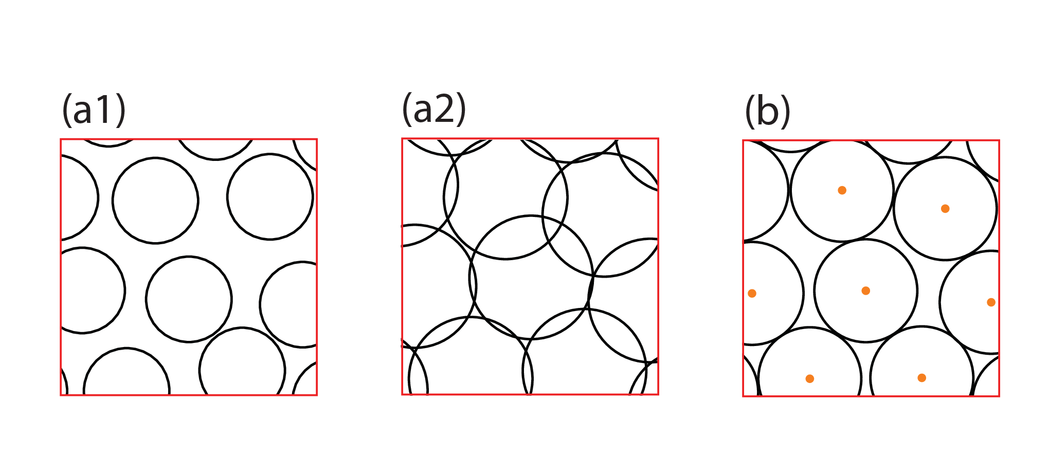
where is the total number of spherical grains in the system. After an initial configuration is generated, we grow (shrink) each sphere by so that the volume fraction of the system increases (decreases) by , if is smaller (greater) than a minimal average potential energy given by the machine precision. Each change of is followed by energy minimization of done by the conjugate gradient (CG) method. During the CG relaxation process, spheres are allowed to move freely. instead of is applied when switching from compression to expansion of the system and vice versa. The procedure of energy minimization following volume perturbation is repeated until to create a packing, where there are only tiny overlaps between spheres and each sphere keeps force balance with all its contact neighbors. The algorithm is schematically shown in figure 1 [18, 19].
The algorithm runs at zero temperature and under zero gravity, so the system is very unlikely to be trapped by global minima such as the fcc or hcp configuration on the potential energy landscape. In some rare cases, the packing algorithm ends up with unstable or ordered configurations, which can be removed manually. The number of grains and volume fraction of the specific sphere packings used to obtain the Voronoi seeds in this study are = , , and , respectively. All these sphere packings are randomly packed, and their ’s are basically the same as the RCP density.
2.2 Algorithm for Voronoi Tessellation
The centers of randomly close packed spheres are used as Voronoi seeds to create Voronoi grains by the standard Voronoi tessellation: the th Voronoi grain contains points that are closer to the th seed than to any other seeds. The Voronoi boundary between the th and th spheres is determined by the relation
| (3) |
where is the distance between a point in the Voronoi boundary to the th sphere of radius . We call Voronoi seeds obtained this way ‘uniform Voronoi seeds’ and the created Voronoi grains ‘uniform Voronoi grains’. In figure 2, it has been shown that the grain size dispersity of uniform Voronoi grains is very small (), compared with that of randomly chosen nonuniform Voronoi grains (), and therefore influence of grain size dispersity is quantitatively negligible. Figure 3 shows the Voronoi tessellations of used specifically in this study. We fill each Voronoi grain with a face-centered cubic (fcc) randomly-oriented crystallite. Using uniform Voronoi seeds guarantees that not a single Voronoi grain is considerably larger or smaller than the average grain size, and each grain is surrounded by grain boundaries with similar geometrical features. In other words, the configuration can be treated as a homogeneous medium down to the characteristic length scale in this study.
Moreover, since the structure is randomly packed, it dismisses the concern that there may exist any artificial slip planes in the system caused by orderly arranged grains with a uniform grain size distribution, which may weaken the stiffness and strength of the system. After an initial configuration is constructed, under zero external loadings, we relax it at the temperature that is also used for the subsequent tensile tests, until the MD extended hamiltonian reaches a stable value. This relaxation process usually takes less than seconds. The new Voronoi-like algorithm is schematically shown in figure 4.


2.3 Molecular Dynamical Simulation of Tensile Tests
Using the Parallel Molecular Dynamics Stencil (PMDS) code [21], we performed three dimensional MD uniaxial tensile tests, with periodic boundary conditions in all directions, on nanocrystalline Cu at . The normal stresses in the and directions perpendicular to the tensile direction are maintained at zero, while the dimensions along these two directions are subjected to free adjustment. The system exists in the isothermal-isostress ensemble [22]. Atoms interact with one another via the embedded atom model (EAM) Mishin potential [23, 24]. The strain-rate in the tensile direction is . Young’s modulus is strain-rate independent though. We calculated the overall Young’s modulus using data in the strain () interval , which is clearly within the linear stress()-strain() region [13].
3 Validation of the Nanocrystalline Model Composed of Randomly Packed Uniform Grains
3.1 Geometrical Properties of the Grain Core and Grain Boundary Components
3.1.1 Identifying Atoms within the Grain Boundaries
In general, atoms located between the interface of two grains are treated as grain boundary atoms. To quantitatively measure the volume fractions of the grain boundary and the grain core components, we use two methods to sort out grain boundary atoms. The first method is calculating coordination number (CN). Here, atom is a neighbour of atom if the distance between them is smaller than , which is defined by the value of the first minimum of the pair distribution function of the system. For Cu at room temperature in our study, . The total number of neighbours of an atom is called the atom’s coordination number. Atoms of are selected as grain boundary atoms and the rest are core atoms. The second method is Common Neighbour Analysis (CNA). In this method, we apply the same for the conventional CNA calculation using LAMMPS [25, 26, 27] and also try the adaptive CNA (a-CNA) calculation using OVITO [28, 29]. Fcc and hexagonal close packed (hcp) atoms are categorized as grain core atoms. Both CNA and a-CNA calculations yield almost the same amounts of grain boundary and grain core atoms.
3.1.2 Measuring the Average Thickness of the Grain Boundaries
Our Voronoi-like protocol generates grains shaped like convex polyhedrons. We approximate these convex polyhedral grains by spheres with an average diameter and an average volume satisfying the relation
| (4) |
where is understood as () if , the total number of the grain core atoms, is obtained by the CN (CNA) calculation, is the total number of Voronoi grains, and is the average volume occupied by a single atom in an fcc or hcp unit cell, which is for Cu at . Throughout our investigation, is always smaller than .
We can define the volume fraction of the grain core as
| (5) |
where is the volume of the simulation supercell. Moreover, we assume that each approximated spherical grain is covered with a grain boundary shell of average thickness . The overall grain boundary thickness of the system is thus , because grain boundary is the space between two adjacent grains (see figure 4(b)). Following the above assumptions, can also be given by the expression
| (6) |
Varying the size of the simulation supercell, we can create a set of , where and can be calculated using equations (4) and (5) separately. Both CN and CNA calculations give similar when . As a result, when greater than this system size, and basically can be used interchangeably and labeled simply as . By fitting the set to equation (6), we can estimate the grain boundary thickness in our system as shown in figure 5. We found that the total fitted grain boundary thickness of the system () is about (CN calculation) and (CNA calculation), which are close to the values () reported in other experimental and simulation studies [4, 30, 31, 32, 33]. We also directly calculated the grain boundary thickness by dividing the total volume of the grain boundary component by the total interfacial area between grains calculated by Voro++ [20]. The thickness is about (CN calculation) and (CNA calculation), as the grain size is , where approaches the coarse-grained limit.

3.1.3 Geometrical Inhomogeneity of the Grain Boundary Component
In figure 6, we show the grain boundary structure. The grain boundary is about two to three atoms thick, translating to for Cu at . We can also observe some geometrical inhomogeneity in the grain boundary region. This is an intrinsic feature of the grain boundary, enhanced by thermal fluctuations when the temperature is above zero. To analyze the sparsity of grain boundary atoms due to this inhomogeneity, we measured the average volume surrounding one atom in the grain boundary, . The value is (CN calculation) and (CNA calculation), which are and larger than , respectively. Moreover, we calculated the average CN of the whole system () and of the grain boundary (). For , we find they are and , respectively, which agrees with a recent experimental study with a similar (, , ) [33].

3.2 Overall Elastic Response
The overall is shown in figure 7 against experimental data [35, 36, 16, 37, 4], and another MD simulation [13] data. The experimental data are obtained within a temperature range of to , however. To compare our simulation data with the experimental ones at different temperatures meaningfully, we measured the temperature-dependence of in our MD tensile tests. The obtained value was , which is almost the same as what had been reported in a previous MD study () [13], but larger than one experimental value () found in the same material with a grain size of [38]. For a temperature change of in simulation, Young’s modulus will vary by , which is also the size of the error bar that should be applied to the simulation data when we make a raw comparison. Similarly, we can calculate the projected values of the experimental data at if the temperature-dependence of is taken into account. The fitted agrees with experimental data extremely well, and approaches the coarse-grained limit [39] when is larger than .

3.3 Flow Stress of Plastic Deformation
Using the uniaxial tensile test at with a strain-rate , we also measured the flow stress taken as the average stress () in the strain () interval between and as a function of . In figure 8, we compare our simulation data of uniform grains with another simulation study, where a set of Voronoi seeds are randomly chosen to create nonuniform grains [10]. Both studies show a transition from regular Hall-Petch to inverse Hall-Petch behavior around grain size . Again, using uniform grains does not introduce extra weakness to our system due to monodispersity of the grain size distribution.
We also verified the isotropy of the system. For (smallest number of grains used in this study) grains of , we measured the elastic moduli and flow stresses in three perpendicular directions; their variations were only and , respectively. For grains, the system contains different grain boundaries, and we believe it behaves isotropically. To make sure there is minimal finite size effect, we measured the elastic moduli and flow stresses of and grains of , and and grains of . The relative variations in the elastic moduli and flow stresses in either case are smaller than and , respectively. In summary, all of the above agreements in the geometric, elastic, and plastic properties, and isotropy and finite size tests indicate that our new Voronoi-like protocol generates reasonably nanocrystalline configurations resembling real structures closely.

4 Analysis of the Elastic Moduli of the Grain Core and Grain Boundary Components
We can express the overall Young’s modulus in terms of , and by rules of mixtures, where and are Young’s moduli of the grain core component and the grain boundary component, respectively. To estimate and , we fitted to the Voigt [40], Reuss [41], and Hill [42] models, representing the upper bound of , the lower bound of , and the arithmetic mean of the previous two models, respectively. The Hill model has been chosen for practical reasons [43]. For a given set of and , and become parameters to be determined by numerical fitting. We tried both the and . The results are listed in Table 1.
| (Unit: ) | Voigt | Hill | Reuss |
|---|---|---|---|
| () | |||
| CN | |||
| CNA | |||
| () | |||
| CN | |||
| CNA |
The Voigt model gives unphysical negative values of in all four cases. Under both definitions of grain boundary atoms, Hill and Reuss models give meaningful numbers worth further consideration. Theoretically, the Reuss model describes the effective moduli of a solid suspension in a matrix of near zero shear modulus, a quantity proportional to the elastic modulus for homogeneous isotropic materials [44]. In Table 1, we found that all ratios of are smaller than , a close scenario to an ideal Reuss example, although the ratio is nonzero. In other words, in our system, grain cores are embedded in a grain boundary matrix with a stiffness of less than about of that of the core part. This result reciprocally justifies the fact that among the three proposed models, the Reuss model best captures the elastic response of our system. Specifically, assuming a linear constitutive relation, the Reuss model can be expressed as
| (7) |
The Reuss fits are shown in figure 9. We choose the results of over , because the values are much closer to the coarse-grained limit, [39].

Knowing , , and , we can rewrite as a function of only by combining equations (6) and (7). The fitted overall is shown in figure 7 compared with other experimental and simulation data [35, 36, 16, 37, 4, 13].
The greater temperature-dependence in our system and the elastic softness of the grain boundary component may be because the volume fraction of the grain boundary increases with decreasing , and the grain boundary is more thermally-sensitive than the grain core, a fact due to the geometrical inhomogeneity in the grain boundary (see the inset of figure 6) [13]. We verify this by looking at atomic scale deformation due to thermal fluctuations of both components at . In figure 10, we show that, locally, the grain boundary deforms more than the grain interior, while both components are subjected to an equal amount of thermal vibrations at the same temperature.

5 Discussions and Conclusions
In this study we investigated Young’s moduli of the grain boundary and the grain core components of fully dense nanocrystalline copper with an average grain size at . We used an isotropic nanocrystalline model that includes not only the most stable grain boundary, but also a general combination of varied grain boundaries generated by our new Voronoi-like algorithm. The seeds of the new Voronoi algorithm, used for creating monodisperse nanocrystalline grains, are centers of randomly close packed identical spheres. The model composed of uniform Voronoi grains, although extremely ideal, faithfully reproduces the geometric, elastic, and plastic features of bulk nanocrystalline copper. We conducted MD uniaxial tensile tests to measure Young’s modulus as a function of .
We found the following key results concerning the stiffness of nanocrystalline Cu at finite temperature: 1) The grain boundary component is less stiff than the grain interior; 2) At , Young’s modulus of the grain boundary component is less than of that of the grain interior, not as generally believed; 3) The grain boundary component is more thermally-sensitive compared with the grain core component, because the grain boundary shows more local deformation compared with the core region under the same thermal fluctuations.
It is important to emphasize here the distinct simplicity of our approach to estimating Young’s moduli at finite temperature. Starting with a nanocrystalline model containing near-spherical monodisperse grains with random crystal orientations, we obtain the grain boundary thickness and its elastic modulus by numerical fits, without making any assumptions about the elastic responses of the grain boundary. Due to unavoidable inaccuracy of numerical fits, we focus on the ratio of Young’s moduli in the grain boundary and the core components, instead of their absolute values. Through our analysis, we argue that the grain boundary is elastically much softer, with less than of the stiffness of the grain interior, at the studied temperature. This striking finding could be explained by the fact that the somewhat disordered grain boundary component is much more thermally sensitive, and it has been verified by observing the structure change under thermal fluctuations (figure 10). Because the CN of the grain boundary component is only slightly smaller ( for , for example) than that of the whole system and the volume shared by a single grain boundary atom is merely to bigger than that of a core atom, it is impressive that a small disorder in structure can create a significant drop in stiffness.
Studies assuming Young’s modulus of the grain boundary to be of the grain interior value usually attribute the observed reduction of the overall elastic modulus to porosity when the grain size is smaller than [5]. The influence of porosity on the elastic properties of nanocrystalline materials at finite temperature is likely overestimated and should be further examined, since we have shown here that the grain boundary is not as stiff as previously believed.
Our results also directly help developing more advanced continuum models. For example, in recent quasi-continuum simulations, it has been shown that if the grain boundary has a very small elastic modulus (17% of the stiffness of the grain core), the shear stress field of the edge dislocation shrinks with grain size [46]. Our study about Young’s modulus in the grain boundary region sheds new light on this result.
Acknowledgments
Financial support from grants for Scientific Research on the Innovative Area of ‘Bulk Nanostructured Metals’ (No. 22102003), Scientific Research (A) (No. 23246025), Challenging Exploratory Research (No. 22656030), Elements Strategy Initiative for Structural Materials (ESISM), and JST under Collaborative Research Based on Industrial Demand (Heterogeneous Structure Control) is gratefully acknowledged. We also thank H. Kimizuka for advice about PMDS code, T. Shimokawa and C. S. O’Hern for their insightful comments, and I. Holca for proofreading the manuscript.
References
- [1] H. Gleiter, Prog. Mater. Sci. 33 (1998) 223.
- [2] H. Gleiter, Acta. Mater. 48 (2000) 1.
- [3] M. A. Meyers, A. Mishra, D. J. Benson, Prog. Mater. Sci. 51 (2006) 427.
- [4] T. D. Shen, C. C. Koch, T. Y. Tsui, G. M. Pharr, J. Mater. Res. 10 (1995) 2892.
- [5] H. S. Kim, M. B. Bush, Nano-structured Materials 11 (1999) 361.
- [6] M. D. Kluge, D. Wolf, J. F. Lutsko, S. R. Phillpot, J. Appl. Phys. 67 (1990) 2370.
- [7] L. Wong, D. Ostrandeer, U. Erb, G. Palumbo, K. T. Aust, Nanophases and Nanocrystalline Structures, The Minerals, Metals & Materials Society, Warrendale, PA, 1994, p. 85.
- [8] T. Masumoto, R. Maddin, Mater. Sci. Eng. 19 (1975) 1.
- [9] D. E. Polk, B. C. Giessen, F. G. Garddner, Mater. Sci. Eng. 25 (1976) 309.
- [10] J. Schiøtz, K. Jacobson, Science 301 (2003) 1357.
- [11] S. Yip, Nature 3 (2004) 11.
- [12] Y. Wang, M. Chen, F. Zhou, E. Ma, Nature 419 (2002) 912.
- [13] J. Schiøtz, T. Vegge, F. D. DiTolla, K. W. Jacobsen, Phys. Rev. B 60 (1999) 11971.
- [14] S. Torquato, T. M. Truskett, P. G. Debenedetti, Phys. Rev. Lett. 84 (2000) 2064.
- [15] Y. Champion, C. Langlois, S. Guérin-Mailly, P. Langlois, J.-L. Bonnentien, M. J. Hy̋tch, Science 300 (2003) 310.
- [16] M. Legros, B. R. Elliott, M. N. Rittner, J. R. Weertman, K. J. Hemker, Philos. Mag. A 80 (2000) 1017.
- [17] J. G. Berryman, Phys. Rev. A 27 (1983) 1053.
- [18] N. Xu, J. Bławzdziewicz, C. S. O’Hern, Phys. Rev. E 71 (2005) 061306.
- [19] G. J. Gao, J. Bławzdziewicz, C. S. O’Hern, Phys. Rev. E 74 (2006) 061304.
- [20] C. H. Rycroft, Chaos 19 (2009) 041111.
- [21] H. Kimizuka, H. Kaburaki, F. Shimizu, J. Li, J. Computer-Aided Materials Design 10 (2003) 143.
- [22] G. J. Martyna, D. J. Tobias, M. L. Klein, J. Chem. Phys. 101 (1994) 4177.
- [23] Y. Mishin, M. J. Mehl, D. A. Papaconstantopoulos, A. F. Voter, J. D. Kress, Phys. Rev. B 63 (2001) 224106.
- [24] T. Frolov, Y. Mishin, Phys. Rev. B 79 (2009) 174110.
- [25] S. Plimpton, J. Comp. Phys. 117 (1995) 1.
- [26] D. Faken, H. Jonsson, Comput. Mater. Sci. 2 (1994) 279.
- [27] H. Tsuzuki, P. S. Branicio, J. P. Rino, Comput. Phys. Commun. 177 (2007) 518.
- [28] A. Stukowski, Modelling Simul. Mater. Sci. Eng. 18 (2010) 015012.
- [29] A. Stukowski, Modelling Simul. Mater. Sci. Eng. 20 (2012) 045021.
- [30] Y. Champion, M. J. Hy̋tch, Eur. Phys. J. Appl. Phys. 4 (1998) 161.
- [31] B. Fultz, H. N. Frase, Hyperfine Interact. 130 (2000) 81.
- [32] A. Pedersen, G. Henkelman, J. Schiøtz, H. Jónsson, New J. Phys. 11 (2009) 073034.
- [33] E. A. Stern, R. W. Siegel, M. Newville, P. G. Sanders, D. Haskel, Phys. Rev. Lett. 75 (1995) 3874.
- [34] J. Li, Modelling Simul. Mater. Sci. Eng. 11 (2003) 173.
- [35] P. G. Sanders, J. A. Eastman, J. R. Weertman, Processing and Properties of Nanocrystalline Materials, The Minerals, Metals & Materials Society, Warrendale, PA, 1996, pp. 379–386.
- [36] P. Sharma, S. Ganti, J. Mater. Res. 18 (2003) 379.
- [37] P. G. Sanders, J. A. Eastman, J. R. Weertman, Acta. Mater. 45 (1997) 4019.
- [38] A. B. Lebedev, Y. A. Burenkov, A. E. Romanov, V. I. Kopylov, V. P. Filonenko, V. G. Gryaznov, Mater. Sci. Eng., A 203 (1995) 165.
- [39] R. W. Hertzberg, Deformation and Fracture Mechanics of Engineering Materials, Wiley, 1996.
- [40] W. Voigt, Lehrbuch der Kristallphysik, Leipzig, 1910.
- [41] A. Reuss, Mathematik und Mechanik 9 (1929) 49.
- [42] R. Hill, Proc. Phys. Soc. A 65 (1952) 349.
- [43] S. Karato, Deformation of Earth Materials, Cambridge University Press, 2008, p. 216.
- [44] P. Avseth, T. Mukerji, G. Mavko, Quantitative Seismic Interpretation, Cambridge University Press, 2005, pp. 5–8.
- [45] F. Shimizu, S. Ogata, J. Li, Materials Transactions 48 (2007) 2923.
- [46] T. Shimokawa, Proceeedings of the Society of Materials Science 55 (2011) 319.