Exotic Ising dynamics in a Bose-Hubbard model
Abstract
We explore the dynamical properties of a one-dimensional Bose-Hubbard model, where two bosonic species interact via Feshbach resonance. We focus on the region in the phase diagram which is described by an effective, low-energy ferromagnetic Ising model in both transverse and longitudinal fields. In this regime, we numerically calculate the dynamical structure factor of the Bose-Hubbard model using the time-evolving block decimation method. In the ferromagnetic phase, we observe both the continuum of excitations and the bound states in the presence of a longitudinal field. Near the Ising critical point, we observe the celebrated mass spectrum in the excited states. We also point out possible measurements which could be used to detect these excitations in an optical lattice experiment.
pacs
67.85.-d, 37.10.Jk , 75.10.Pq, 75.78.FgThe search for emergent excitations arising from strong correlations has been very fruitful over the past few decades, from fractional quasiparticles in the fractional quantum Hall effect [1], to effective magnetic monopoles in spin ice [2]. The one-dimensional (1D) transverse-field Ising model is another famous case showing collective excitations [3]. It is a paradigmatic model for quantum phase transitions, hosting a critical point with central charge [4]. Zamolodichkov showed that, by perturbing such a critical theory with a symmetry-breaking field, eight massive particles emerge in the excitation spectrum [5]. These particles are the hallmark of an underlying continuous symmetry, a very complex symmetry group discovered in mathematics, which attracts much interest in a wide community, see e.g. Ref. [6]. The ratio between the masses of the two lightest particles predicted by symmetry has been recently observed by Coldea et al. in neutron-scattering studies of the quantum magnet CoNb2O6 [7].
The quest for complex many-body phenomena and unconventional excitations has greatly benefited from advances in ultracold atomic gases [10, 8]. By confining the atomic cloud to an optical lattice, it is now possible to explore strongly-interacting lattice models with an unprecedented degree of control and tunability [9]. Important milestones include the observation of the superfluid to Mott insulator transition in bosonic systems [11] and the antiferromagnetic 1D Ising transition on a tilted optical lattice [12]. Due to their long coherence times and the possibility of tuning the parameters of the system, cold atoms in optical lattices also allow the study of non-equilibrium dynamics [13, 14] – which is usually very difficult in a condensed-matter setting. A promising research area is the use of multi-component atomic mixtures as a route to effective magnetic models, see e.g. Refs. [15, 16]. More specifically, recent theoretical work has proposed mixtures of atoms and molecules near a Feshbach resonance [17] in a Mott state as a route to the 1D Ising model [18, 19, 20]. Here, the Feshbach resonant coupling between different species acts as a tunable handle on quantum fluctuations.
In this paper, we study the low-energy dynamical properties of a 1D Bose-Hubbard model describing two different bosonic species coupled by Feshbach resonance in the Mott insulating regime. We obtain the low-energy spectrum of this model via an appropriate dynamical structure factor. The characteristic signatures of the broken-symmetry and disordered phases are clearly observed. We reach an excellent agreement with the excitation spectrum of the Ising model. By tuning the bosonic system close to a perturbed critical point, its excitation spectrum reveals the signatures of symmetry.
We consider the following pairing Bose-Hubbard Hamiltonian, previously studied in [21, 23, 22, 24, 25, 18, 19, 20, 26, 27],
| (1) |
describing two species of bosons on a 1D lattice, where . Atoms are labeled by while molecules are labeled by . Here are on-site potentials, are hopping parameters between nearest-neighbour sites, and are on-site interactions. Two atoms form a molecule via -wave pairing, driven by Feshbach coupling . The Feshbach interaction breaks the independent conservation of the number of atoms and molecules, but the total number is conserved. We work in the canonical ensemble, by keeping the total density fixed.
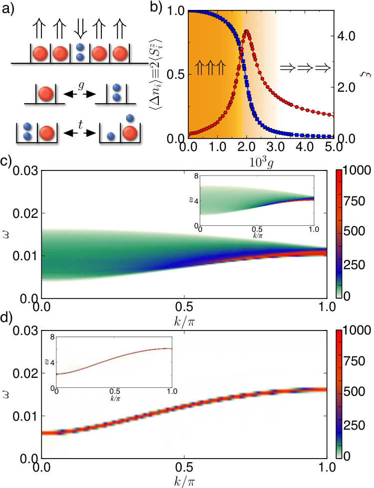
The low-energy behaviour of the Hamiltonian Eq. (1) in the Mott regime with can be conveniently described with the aid of an effective 1D quantum Ising model [18, 19, 20], which is also helpful in guiding us to the regions of interest. The “effective spin” degrees of freedom are and in the occupation basis , see Fig. 1(a). We truncate the Hilbert space to a maximum of three atoms and one molecule per site, which is already a good approximation to canonical soft-core bosons for the large limit considered here [20]. This choice allows the hopping of atoms, even if a pair is already present on a site. The effective Ising model (up to an additive constant) is obtained via a strong-coupling expansion around the small-hopping limit
| (2) |
The effective spin operators have a direct interpretation in terms of bosons,
| (3) |
measures the imbalance in the density of bosons at site , while
| (4) |
accounts for inter-species fluctuations. At a qualitative level, the Ising exchange interaction arises from the motion of bosons, the longitudinal field tunes an overall imbalance between the two species, and the transverse field controls the fluctuations between the two species, cf. Fig. 1(a).
We find the ground state of the full Hamiltonian Eq. (1) using a variant of the infinite density-matrix renormalization group (iDMRG) method [28, 29], yielding a matrix-product-state (MPS) representation of the ground-state wave-function in the thermodynamic limit. We find that matrix bond dimensions are enough to describe the ground states studied, with a truncation error up to . The time-evolving block decimation (TEBD) method [30, 31] is then used to calculate a dynamical structure factor function of the bosonic model, following the general strategy laid out in Refs. [32, 33, 34, 35]. This function measures the response to fluctuations between the two species, corresponding to the operator in the Ising language:
| (5) |
The two-point dynamical correlation function
| (6) |
is calculated with a real-time evolution of the ground-state MPS after is applied to a given site, and its Fourier transform yields . The sampled time is extended by extrapolating with linear prediction [36]. We stop the simulation once the “light-cone” of local correlations gets close to the boundary of a fixed window size (typically ), ensuring that our simulations do not suffer from finite-size effects [35]. Since the low-energy dynamics are set by the effective model, the “light-cone” and the entanglement entropy grow very slowly with time. Hence, we are able to reach extremely large times, up to , while keeping the truncation error down to by setting . We have checked the convergence of our results with the Trotter time step , settling on .
The ground-state properties of the pairing Bose-Hubbard model have been studied recently [24, 25, 18, 19, 20]. While, previously, emphasis was placed on the region of the phase diagram where the effective model is the antiferromagnetic Ising chain, here we focus on parameters yielding an effective ferromagnetic model.
In order to make contact with previous work, we impose the following constraints : , , and — thus the energy scale is set by the on-site interaction. The parameters of the corresponding Ising Hamiltonian Eq. (2) are then found through the strong-coupling expansion [20]
| (7) | ||||
| (8) | ||||
| (9) |
We choose a representative value of (), which avoids a slow down in the dynamics at lower values of . Eq. (8) predicts that the effective longitudinal field is canceled by tuning . However, even after this, we observe in our simulations the effects of the presence of an effective longitudinal field, which arises from contributions in perturbation theory in small beyond the second-order expansion considered in Ref. [20]. Rather than extending this calculation to higher order, we add an extra perturbation, , to the molecular potential in Eq. (8) to compensate for this “stray” longitudinal field. In general, this term depends on the values of and chosen. Probably, this is also a more realistic way of achieving the same result in an experimental setting, since it just involves further fine-tuning of , instead of balancing a version of Eq. (8) with more, higher-order, terms.
The resulting phase diagram, where the Feshbach coupling is the only free parameter and the order parameter is , is shown in Fig. 1(b) for . For low values of an ordered phase based on the product state with one molecule localised per site, , is found. The stray longitudinal field described above biases the system towards this state, rather than the “atomic” ordered state based on two atoms localised per site, . All of the physical behaviour described here still holds in the case where the on-site potentials have been tuned to favour the atomic ground state. By increasing the value of the system goes through a crossover into a disordered phase. This crossover is revealed by the non-diverging peak of the correlation length near (), indicating that the Ising critical point is nearby.
The low-energy excitation spectrum is revealed by the transverse dynamical structure factor function . The energy scales observed here are set by the effective Ising parameters and are hence rather low with . This is well below the Mott gap , above which single-particle excitations appear. We start with the “molecular” ground state where the excitation in Eq. (6) dissociates one molecule into two atoms at site , i.e. flips . Evolution in time creates a domain of atoms, which is a bound state of two domain walls propagating in opposite directions. In the absence of a longitudinal field, the domain walls are deconfined as the two ground states are perfectly degenerate. This is achieved by setting () and fine tuning the on-site potential . The dynamical structure factor function, shown in Fig. 1(c), displays a broad continuum of excitations around , sharpening closer to the Brillouin zone edge at . The agreement with the pure Ising model is very good, as shown by the matching of the onset of the continuum in the Bose-Hubbard model with the energy of the lowest excitation (dashed line), of the transverse-field Ising chain with . The Ising is also shown in the inset, see Ref. [3, 32].
A finite longitudinal field confines the domain walls, destroying the continuum of excitations, except for resonances at specific momenta and energies, which can be seen as massive “meson” bound states [37]. An effective longitudinal field has the same effect here, breaking up the continuum observed in Fig. 1(c) (not shown).
The dynamical structure factor in the disordered phase for large is shown in Fig. 1(d) for a representative value (). A well-defined quasi-particle with a quadratic dispersion is visible, which can be identified with the single spin-flip excitation of the Ising chain in the disordered phase, see dashed line inset.
The most impressive feature of the Ising model is the symmetry [3], which is revealed when it is tuned to the critical point with a longitudinal field applied. This is described by the perturbation of a conformal field theory, which is still integrable and leads to exactly eight massive bound states, whose mass ratios are known analytically [5].
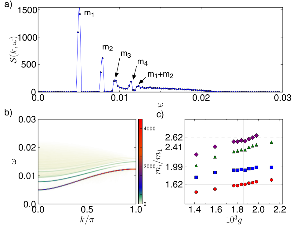
The mass ratio between the two lightest particles is the golden ratio and has been experimentally observed in CoNb2O6 [7]. However, heavier excitations are difficult to measure there, since they are located within the continuum. Furthermore, it is not possible to modify this by tuning the longitudinal field, which is fixed by the inter-chain coupling. We now tune the parameters in our bosonic model to this interesting region. The excitation spectrum of the system close to the perturbed Ising critical point, with () and ), is revealed by examining the dynamical structure factor function in Figs. 2(a,b). At least five different excitations are clearly identified above the continuum, which we can associate with the first four particles of the theory and the bound-state pair . In Fig. 2(c) we present a sweep in Feshbach coupling near this point, while keeping the molecular potential perturbation fixed at for better convergence of the results. The mass ratios calculated in this region are very close to the analytically predicted ones (horizontal lines), crossing them for a value of (). The observation of this highly non-trivial sequence in the energy spectrum is a clear evidence for the emergence of symmetry in a Bose-Hubbard model. This small renormalisation of the critical value of probably arises from contributions in higher order from perturbation theory. The different mass ratios increase roughly linearly with . The heaviest particles become progressively more difficult to observe with increasing , since their spectral weight decreases. The ratios obtained do not change significantly when the molecular potential perturbation is doubled to , staying within error bars of the data points in Fig. 2(c). The stability of the results for such a large ratio of fields, , matches that observed in the Ising chain [32].
Recent developments in Bragg spectroscopy applied to cold atoms allow the study of the full excitation spectrum, resolved in momentum and energy, even in the presence of an optical lattice [38, 39]. A complementary, and simpler, scheme for observing some of the behaviour described here is also desirable. Motivated by recent experimental [40] and theoretical work [41, 42], we now look at the propagation of a single excitation in space and time. We prepare the system in the molecular ground state for , apply the dissociation excitation at a site , and track the evolution in time of the relative local density at a site .
The effective longitudinal field has been tuned to by setting in Fig. 3(a). At a qualitative level, drops suddenly when a domain wall reaches site , signalling the dissociation of the molecule at that site () into two atoms (). Since there is no effective longitudinal field to confine the domain walls, the domain persists in the long-time limit, and it grows with more sites being progressively flipped, leading to the continuum of excitations in the dynamical structure factor shown in Fig. 1(c). The behaviour in the presence of an effective longitudinal field, , is shown in Fig. 3(b). The domain of atoms still grows up to a few sites away from . However, the induced confining potential inhibits the propagation of the domain walls and the domain quickly collapses. The sites which were excited eventually return to a state with in the long-time limit, which is different from the original molecular ground state.
Systems of hundreds of cold atoms confined to 1D optical lattices have been extensively explored in the last decade [8, 17], including heteronuclear bosonic mixtures [43, 44] which can be described by Bose-Hubbard models similar to Eq. (1), see e.g. Ref. [45]. The key requirements to observe the behaviour described here are the formation of a symmetry-breaking insulating phase and the presence of fluctuations able to destroy it. The presence of a trap potential should not affect much the results, as long as the central insulating domain with is large enough. In order to ensure an insulating phase, the ratios , which depend on the lattice depth and the intra-species scattering length, should be . Biasing the on-site potentials , controls the effective longitudinal field , and therefore the stability of the particles and their spectral weight relative to the continuum. The Feshbach coupling is itself an effective term depending, among others, on the background scattering length and the width of the resonance [23, 17]. The effective Ising interaction in Eq. (2) is controlled by the ratios between the different , including , which is the term freely adjustable in Feshbach resonance experiments by the detuning of the magnetic field away from the resonance value [17, 45]. In this way the and ratios could be controlled, allowing a sweep near the critical point as in Fig. 3(c), in order to find the optimal set of parameters corresponding to symmetry.
In conclusion, we have shown that the low-energy excitations of a 1D Bose-Hubbard pairing model can faithfully simulate the dynamical properties of the quantum Ising chain. We find the characteristic Ising features in the low-energy spectrum, such as the incoherent continuum, quadratic quasi-particles, and, above all, massive excitations emerging from symmetry. Recent developments in manipulating systems described by models such as Eq. (1), and in accessing the low-energy excitation spectrum, open up the fascinating possibility of realising this behaviour in a cold atoms experiment.
We are grateful to M. J. Bhaseen and F. H. L. Essler for introducing us to this interesting model. We thank J. Eisert, S. Ejima, H. Fehske, J. A. Kjäll, A. M. Turner and M. Zaletel for fruitful discussions.
References
- [1] R. B. Laughlin, Phys. Rev. Lett. 50, 1395 (1983).
- [2] C. Castelnovo, R. Moessner, and S. L. Sondhi, Nature 451, 42 (2008).
- [3] G. Mussardo, Statistical Field Theory (Oxford University Press, 2010).
- [4] S. Sachdev, Quantum Phase Transitions (Cambridge University Press, London, 1999).
- [5] A.B. Zamolodchikov, Int. J. Mod. Phys. A4, 4235 (1989).
- [6] D. Vogan, Not. AMS, 54, (9), 1022 (2007).
- [7] R. Coldea, D. Tennant, E. Wheeler, E. Wawrzynska, D. Prabhakaran, M. Telling, K. Habicht, P. Smeibidl, and K. Kiefer, Science 327, 177 (2010).
- [8] I. Bloch, J. Dalibard, and W. Zwerger, Rev. Mod. Phys. 80, 885 (2008).
- [9] D. Jaksch, C. Bruder, J. I. Cirac, C. W. Gardiner, and P. Zoller, Phys. Rev. Lett. 81, 3108 (1998).
- [10] M. Lewenstein, A. Sanpera, V. Ahufinger, B. Damski, A. Sen, and U. Sen, Advances in Physics 56, 243 (2007).
- [11] M. Greiner, O. Mandel, T. Esslinger, T. W. Hänsch, I. Bloch, Nature 415, 39 (2002).
- [12] J. Simon, W. S. Bakr, R. Ma, M. E. Tai, P. M. Preiss, and M. Greiner, Nature 472, 307 (2011).
- [13] M. Cheneau, P. Barmettler, D. Poletti, M. Endres, P. Schausz, T. Fukuhara, C. Gross, I. Bloch, C. Kollath, and S. Kuhr, Nature 481, 484 (2012).
- [14] S. Trotzky, Y. A. Chen, A. Flesch, I. P. McCulloch, U. Schollwöck, J. Eisert, and I. Bloch, Nature Physics 8, 325 (2012).
- [15] L.-M. Duan, E. Demler, and M. D. Lukin, Phys. Rev. Lett. 91, 090402 (2003).
- [16] A. B. Kuklov and B. V. Svistunov, Phys. Rev. Lett. 90, 100401 (2003).
- [17] C. Chin, R. Grimm, P. Julienne, and E. Tiesinga, Rev. Mod. Phys. 82, 1225 (2010).
- [18] M. J. Bhaseen, A. O. Silver, M. Hohenadler, and B. D. Simons, Phys. Rev. Lett. 103, 265302 (2009).
- [19] M. Hohenadler, A. O. Silver, M. J. Bhaseen, and B. D. Simons, Phys. Rev. A 82, 013639 (2010)
- [20] M. J. Bhaseen, S. Ejima, M. Hohenadler, A. O. Silver, F. H. L. Essler, H. Fehske, and B. D. Simons, Phys. Rev. A 84, 023635 (2011).
- [21] L. Radzihovsky, J. Park, and P. B. Weichman, Phys. Rev. Lett. 92, 160402 (2004).
- [22] K. Sengupta and N. Dupuis, Europhys. Lett. 70, 586 (2005).
- [23] D. B. M. Dickerscheid, U. Al Khawaja, D. van Oosten, and H. T. C. Stoof, Phys. Rev. A 71, 043604 (2005).
- [24] V. G. Rousseau and P. J. H. Denteneer, Phys. Rev. A 77, 013609 (2008).
- [25] V. G. Rousseau and P. J. H. Denteneer, Phys. Rev. Lett. 102, 015301 (2009).
- [26] S. Ejima, M. J. Bhaseen, M. Hohenadler, F. H. L. Essler, H. Fehske, and B. D. Simons, Phys. Rev. Lett. 106, 015303 (2011).
- [27] M. J. Bhaseen, S. Ejima, F. H. L. Essler, H. Fehske, M. Hohenadler, and B. D. Simons, Phys. Rev. A 85, 033636 (2012).
- [28] I. P. McCulloch, arXiv:0804.2509 (2008).
- [29] J. A. Kjäll, M. P. Zaletel, R. S. K. Mong, J. H. Bardarson, and F. Pollmann, Phys. Rev. B 87, 235106 (2013).
- [30] G. Vidal, Phys. Rev. Lett. 91, 147902 (2003).
- [31] G. Vidal, Phys. Rev. Lett. 98, 070201 (2007).
- [32] J. A. Kjäll, F. Pollmann, and J. E. Moore, Phys. Rev. B 83, 020407 (2011).
- [33] A. Milsted, J. Haegeman, T. J. Osborne, and F. Verstraete, arXiv:1207.0691 (2012).
- [34] V. Zauner, M. Ganahl, H. G. Evertz, and T. Nishino, arXiv:1207.0862 (2012).
- [35] H. N. Phien, G. Vidal, and I. P. McCulloch, Phys. Rev. B 86, 245107 (2012).
- [36] S. R. White and I. Affleck, Phys. Rev. B 77, 134437 (2008).
- [37] B. M. McCoy and T. T. Wu, Phys. Rev. D 18, 1259 (1978).
- [38] D. Clément, N. Fabbri, L. Fallani, C. Fort, and M. Inguscio, Phys. Rev. Lett. 102, 155301 (2009).
- [39] P. T. Ernst, S. Götze, J. S. Krauser, K. Pyka, D.-S. Lühmann, D. Pfannkuche, and K. Sengstock, Nature Phys. 6, 56 (2010).
- [40] J. F. Sherson, C. Weitenberg, M. Endres, M. Cheneau, I. Bloch, and S. Kuhr, Nature 467, 68 (2010).
- [41] A. Kleine, C. Kollath, I. P. McCulloch, T. Giamarchi, and U. Schollwöck, Phys. Rev. A 77, 013607 (2008).
- [42] J. Honer, J. C. Halimeh, I. McCulloch, U. Schollwöck, and H. P. Büchler, Phys. Rev. A 86, 051606 (2012).
- [43] G. Thalhammer, G. Barontini, L. De Sarlo, J. Catani, F. Minardi, and M. Inguscio, Phys. Rev. Lett. 100, 210402 (2008).
- [44] J. Catani, G. Barontini, G. Lamporesi, F. Rabatti, G. Thalhammer, F. Minardi, S. Stringari, and M. Inguscio, Phys. Rev. Lett. 103, 140401 (2009).
- [45] M. Dalmonte, E. Ercolessi, M. Mattioli, F. Ortolani, and D. Vodola, Eur. Phys. J. Spec. Top. 217, 13 (2013).