Hadron production and QGP Hadronization in Pb–Pb collisions at $\sqrt{s_{NN}}=2.76$ TeV

Preprint: CERN-PH-TH/2012-262

Michal Petráň^1,3 Affiliation:
¹Department of Physics, The University of Arizona, Tucson, Arizona 85721, USA Jean Letessier² Affiliation:
¹Department of Physics, The University of Arizona, Tucson, Arizona 85721, USA Vojtěch Petráček³ Affiliation:
¹Department of Physics, The University of Arizona, Tucson, Arizona 85721, USA Johann Rafelski^1,4 Affiliation:
¹Department of Physics, The University of Arizona, Tucson, Arizona 85721, USA Affiliation: ²Laboratoire de Physique Théorique et Hautes Energies, Université Paris 6, Paris 75005, France Affiliation: ³Czech Technical University in Prague, Faculty of Nuclear Sciences and Physical Engineering Affiliation: ⁴Theory Division of Physics Department, CERN, CH-1211 Geneva 23, Switzerland

March 8, 2013

Abstract

We show that all central rapidity hadron yields measured in Pb–Pb collisions at $\sqrt{s_{NN}}=2.76$ TeV are well described by the chemical non-equilibrium statistical hadronization model (SHM), where the chemically equilibrated QGP source breaks up directly into hadrons. SHM parameters are obtained as a function of centrality of colliding ions, and we compare CERN Large Hadron Collider (LHC) with Brookhaven National Laboratory Relativistic Heavy Ion Collider (RHIC) results. We predict yields of unobserved hadrons and address anti-matter production. The physical properties of the quark–gluon plasma fireball particle source show universality of hadronization conditions at LHC and RHIC.

pacs

25.75.Nq, 24.10.Pa, 25.75.-q, 12.38.Mh

I Introduction and motivation

CERN-PH-TH/2012-262

Our interest in the multi-particle production process in ultra-relativistic heavy ion collisions originates in the understanding that the transverse momentum integrated rapidity distributions are insensitive to the very difficult to fully characterize transverse evolution dynamics of the hot fireball source [1]. A successful description of central rapidity particle yields in a single freeze-out model [2, 3] will be used here to characterize the properties of the hadronizing quark–gluon plasma (QGP) fireball. The QGP breakup, as modeled within the statistical hadronization model (SHM), assumes equal reaction strength in all hadron particle production channels. Therefore, the phase space volume determines the hadron yields. SHM has been described extensively before and we refer the reader to SHARE manuals [4] for both, further theoretical details, and numerical methods. Here, we apply SHM to study particle production in Pb–Pb collisions at $\sqrt{s_{NN}}=2.76\,{\rm TeV}$ (LHC2760), a new energy domain an order of magnitude higher than previously explored in Au–Au collisions at $\sqrt{s_{NN}}=200$ GeV (RHIC200).

We begin by demonstrating that the chemical non-equilibrium SHM variant describes the experimental LHC-ion data with high accuracy. This finding disagrees with claims that SHM alone does not describe the particle multiplicity data obtained in relativistic heavy ion collisions at LHC [5, 6]. In the chemical non-equilibrium SHM approach, we allow quark pair yield parameter $\gamma_{q}$ for light quarks, a feature we presented as necessary model refinement for the past 15 years [7, 8, 9]. We demonstrate the general model validity in our numerical approach by showing correspondence of chemical equilibrium SHM results with other fits to the LHC data. This demonstrates that several SHM programs, which had years time to mature and evolve, are compatible in their data tables of hadronic resonance mass spectra and decay patterns. However, only our extended SHARE-code includes advanced features, such as chemical non-equilibrium of all quark yields, differentiation of up and down quarks, evaluation of fireball physical properties, and the capability to constrain the fit by imposing physical properties on the particle source.

To demonstrate that our chemical non-equilibrium SHM works at LHC, we show in the left panel of figure 1 our fit to the 0–20% centrality data, shown in the second column of table 1, recently presented and studied by the experiment ALICE [5, 6]. Only in this one instance, we consider the relatively wide centrality trigger of 0–20% to compare directly with the earlier analysis effort. As can be seen in the left panel of figure 1, our non-equilibrium SHM approach describes these data with $\chi^{2}/\mathrm{ndf}=9.5/9\simeq 1$ . We see, in figure 1a insert, that the chemical equilibrium SHM works poorly, $\chi^{2}/\mathrm{ndf}=64/11\simeq 6$ , which is the same finding and conclusion as in [5, 6].

While the equilibrium SHM disagrees at LHC across many particle yields the most discussed data point is the p $/\pi=0.046\pm 0.003$ ratio [6], a point we will study in more detail in subsection III.2. Our work shows that the inability of the equilibrium SHM alone to fit the experimental value of p/ $\pi$ ratio does not mean that all variants of SHM do not describe particle production in heavy ion collisions at LHC. One of the key findings of this work is that the chemical non-equilibrium SHM variant without any additional post-hadronization evolution provides an excellent description of all data. We will also argue that the present day hybrid models, that is models which combine SHM results with post-hadronization hadron yield evolution, need to address key features of the data such as quasi-constancy of the p/ $\pi$ ratio as a function of centrality of the heavy ion collision and the abundance of multi-strange baryons.

Refer to caption — Figure 1: (color online) SHM fit to experimental data measured by the ALICE experiment in Pb–Pb collisions at $\sqrt{s_{NN}}=2.76$ TeV for 0–20% centrality (panels (a) and (b) on left hand side) and for 1/4 of this range, 5–10% (panels (c) and (d) on right hand side). The input set of particle types is the same as can be seen in particle listing on the ordinate of panels (b) and (d), in panel (d) also particle yield ratios are used. In the lower panels (b) and (d) comparison of SHM chemical non-equilibrium fit (horizontal line) with data is shown. The experimental data is shown as filled square, in the panel (d) the interpolated experimental data is shown with open symbols (see appendix A for details). The upper panels (a) and (c) show the ratio of model values to experimental data for the three SHM variants and present the key parameter values for: chemical non-equilibrium (solid squares), chemical semi-equilibrium (solid circles) and chemical equilibrium (solid triangles). For readability anti-particles are omitted in panels (a) and (c).

The chemical non-equilibrium results for the 5–10% centrality bin (containing interpolated data, open symbols) is shown for comparison in the right panel of figure 1. The fit has the same set of particles as the 0–20% centrality bin, however, we must fit here three ratios for which data are directly (or by interpolation) available, and we use a more recent set of proton, pion and kaon data. Definition of the model and some technical details about how we obtain results seen in figure 1 follow below; the fitted data are shown in the fourth column of table 1. The figure 1c shows the SHM parameters and $\chi^{2}$ for all three variants. Comparing the SHM parameters on left and right-hand of figure 1 we see a large change in $V$ expected for different centralities. We see that use of finer centrality binning and more mature data sample reduces $\chi^{2}$ for all SHM variants.

As figure 1 shows and we discuss below in detail, the chemical non-equilibrium SHM works perfectly at LHC, resulting in a high confidence level. This could be predicted considering prior CERN Super Proton Synchrotron (SPS) and RHIC data analyses [10, 11, 12], which strongly favor chemical non-equilibrium variant of SHM. Moreover, the chemical non-equilibrium SHM has a dynamical physical foundation in sudden breakup of a QGP fireball, we are not aware of a dynamical origin of the simple chemical equilibrium SHM since no dynamical computation of relativistic heavy ion scattering achieves the chemical equilibrium condition without introduction of unknown particle, cross sections, etc.. Furthermore, as we will discuss in subsection III.3, we obtain hadronization universality across a wide collision energy range: comparing RHIC62 with LHC2760 we show that the fireball source of particles is nearly identical, and consistent with chemically equilibrated QGP fireball. Given this result, chemical non-equilibrium SHM variant is validated across a wide energy range, while the chemical equilibrium SHM [13, 14, 15, 16, 17, 18] is invalidated by the LHC data and this conclusion can be extended across different reaction energies as there is no reason why a model should work only sporadically.

We have now shown that the chemical non-equilibrium is the necessary ingredient in the SHM approach to the process of hadronization of a QGP fireball. The non-equilibrium SHM was proposed when first strange hadron multiplicity results were interpreted more than 20 years ago [19]. The yield of strange hadrons indicated that the number of quark pairs present had to be modified by a factor $\gamma_{s}$ , the source of strangeness is not populating the final state hadrons with the yields expected from the hadronic chemical equilibrium, a point of view widely accepted today. At SPS energies, for which this model was originally conceived, production of strangeness did not yet saturate the QGP phase space, that is strangeness was out of chemical equilibrium both in QGP fireball source with $\gamma_{s}^{\rm Q}<1$ , and thus also in the final hadronic state with also $\gamma_{s}^{\rm H}<1$ . The distinction of QGP as initial and the final hadron phase space domain for $\gamma_{s}$ was also modeled [20]. It is important to always remember that hadron phase space non-equilibrium can arise from a QGP fireball with strangeness in chemical equilibrium, since, in general, the QGP and hadron phase space strangeness density are greatly different. Moreover, it is quite possible that a not yet in chemical equilibrium QGP, which is the higher density phase, produces an equilibrated hadron yield. This can, however, happen only accidentally and variation of reaction energy or collision centrality shows this.

Another non-equilibrium parameter $\gamma_{c}$ , similar to $\gamma_{s}$ , was introduced very soon after $\gamma_{s}$ to control the charm final state phase space [20], and it has been widely adopted in consideration of a strong charm yield overabundance above chemical hadron gas equilibrium. Note that both strangeness and charm flavors are therefore assumed to have been produced in a separate and independent process before hadronization — and note further that each of the production mechanisms, in this case, is different with charm originating in first parton collisions and strangeness being also abundantly produced in secondary thermalized gluon fusion reactions. At the end of QGP expansion, these available and independently established strangeness and charm particle supplies are distributed into available final state phase space cells, that is the meaning of SHM in a nutshell.

The full chemical non-equilibrium is introduced by means of the parameter $\gamma_{q}\neq 1$ . This situation arises when the source of hadrons disintegrates faster than the time necessary to re-equilibrate the yield of light quarks present. The two pion correlation data provide experimental evidence that favors a rapid breakup of QGP with a short time of hadron production [21], and thus favors very fast, or sudden, hadronization [22, 23]. In this situation, a similar chemical non-equilibrium approach must be applied to the light quark abundance, introducing the light quark phase space occupancy $\gamma_{q}$ . This proposal made for the high energy SPS data [7, 8], helped improve the understanding of RHIC200 hadron rapidity yield results [10] and allowed a consistent interpretation of these data across the full energy range at SPS and RHIC200 [11].

For more than a decade we have made continued effort to show that a high quality (low $\chi^{2}$ ) and simple (no need for hybrid models) description of hadron abundances emerges using chemical non-equilibrium SHM. However, the recognition of the necessity of light quark $(u,d)$ chemical non-equilibrium, i.e., $\gamma_{q}\neq 1$ , remains sparse, despite consistency of this approach with the two pion correlation results which provides additional evidence for fast hadronization [21]. The recent steady advances of lattice QCD [24, 25, 26, 27] favors QGP hadronization at a temperature below the once preferred $T_{c}=165\,\mathrm{MeV}$ temperature. As already noted the equilibrium SHM variant imposing $\gamma_{q}=1$ light quark chemical equilibrium [13, 14, 15, 16, 17, 18] produces (relatively dense) particle chemical freeze-out near to $T=155\,\mathrm{MeV}$ . Such freeze-out assumes on one hand in the present context a relatively high QGP hadronization temperature, and on the other hand requires as a complement an ‘afterburner’ describing further reaction evolution of some particles. As we will argue in section III.2, such ‘hybrid’ model does not result in a viable description of the precise ALICE experimental data.

This is the case since the LHC2760 experimental environment has opened a new experimental opportunity to investigate in detail the SHM hadron production model. Precise particle tracking near to interaction vertex in the ALICE experiment removes the need for off-line corrections of weak interaction decays, and at the same time vertex tracking is enhancing the efficiency of track identification, increasing considerably the precision of particle yield measurement [5, 28]. All data used in the present work was obtained in this way by the LHC-ALICE experiment for Pb–Pb collisions at $\sqrt{s_{NN}}=2.76$ TeV, limited to the central unit of rapidity interval $-0.5<y<0.5$ . The experimental particle yield results are reported in different collision centrality bins according to the geometric overlap of colliding nuclei, with the ‘smallest’, e.g., 0–5% centrality bin corresponding to the nearly fully overlapping geometry of the colliding nuclei. Collision geometry model [29] relates the centrality trigger to the number of participating nucleons $N_{\rm part}$ which we use as our preferred centrality variable in what follows.

Section II presents our general method and approach to the particle multiplicity data analysis. Following a brief summary of the SHM methods in subsection II.1, we describe in subsection II.2 our centrality study of particle production based on the following data: for the 0–20% centrality bin, we obtain the preliminary data from [5, 28]. For the centrality study of particle production, we present in table 1 the final yields of $\pi^{\pm}$ , K^± and p^± as presented in [30]. The preliminary ratio $\phi/$ K, is from [31]; these 7 data points are binned in the same centrality bins and are used as presented. However, several other particle types require rebinning with interpolation and, at times, extrapolation which is further discussed in appendix A. The (preliminary) data input into this rebinning for K ${}^{*0}/$ K^- and for ${2\Lambda}/{(\pi^{-}\!\!+\pi^{+})}$ are also taken from Ref. [31]. Using the preliminary enhancement factors of $\Xi^{-}$ , $\overline{\Xi}^{+}$ , $\Omega^{-}$ , $\overline{\Omega}^{+}$ shown in Ref. [32, 33], combined with yields of these particles for p–p-reactions at $\sqrt{s_{NN}}=7$ TeV as presented in Ref. [34], we obtain the required yield input, see appendix A. In subsection II.3, we present particles both fitted and predicted by SHM, including anti-matter clusters.

In section III, we discuss the key physics outcome of the fits, i.e., the resulting SHM parameters as a function of centrality. We compare to the equilibrium approach in subsection III.1. We discuss the differences seen between the SHM variants and compare our results to our analysis of Au–Au collisions at $\sqrt{s_{NN}}=62.4\,{\rm GeV}$ at RHIC62, as it is a system we analyzed in detail recently [12]. We obtain the bulk physical properties: energy density, entropy density, and pressure, as a function of centrality in subsection III.3, where we also address strangeness and entropy yields. This study is made possible since all SHM parameters are determined with minimal error in consideration of the precise experimental particle multiplicity result. We discuss how our results relate to the lattice-QCD study of QGP properties in subsection III.4. We close our paper with a short summary and discussion of all results in section IV.

II SHM and particle production

II.1 Generalities

We use here SHM implementation within the SHARE program [4]. The SHM describes the yields of particles given the chemical freeze-out temperature $T$ and overall normalization $dV/dy$ (as the experimental data are available as $dN/dy$ ). We account for the small asymmetry between particles and anti-particles by fugacity factors $\lambda_{q},\,\lambda_{s}$ and the light quark asymmetry $\lambda_{I3}$ , see Ref.[4]. We further note that it is not uncommon to present the particle–anti-particle asymmetry employing the baryo-chemical and strangeness chemical potentials defined by

\mu_{B}=3T\ln\lambda_{q}\quad\text{and}\quad\mu_{S}=T\ln(\lambda_{q}/\lambda_{s}),

(1)

the ‘inverse’ definition of $\mu_{S}$ with reference to $\lambda_{s}$ has historical origin and is source of frequent error.

For each value of $\lambda_{q}$ , strangeness fugacity $\lambda_{s}$ is evaluated by imposing the strangeness conservation requirement $\langle s\rangle-\langle\bar{s}\rangle\simeq 0$ . From now on, we omit the bra-kets indicating grand canonical average of the corresponding summed particle yield. The isospin fugacity factor $\lambda_{I3}$ is constrained by imposing the charge per baryon ratio present in the initial nuclear matter state at initial instant of the collision. We achieve this objective by fitting these conservation laws along with particle yield data, using the following form:

	$\displaystyle\frac{s-\overline{s}}{s+\overline{s}}$	$\displaystyle=0.00\pm 0.01,$		(2)
	$\displaystyle\frac{Q-\overline{Q}}{B-\overline{B}}$	$\displaystyle=0.38\pm 0.02.$		(3)

We believe that implementing conservation laws as data points with errors accounts for possibility that particles escape asymmetrically from the acceptance domain.

In the LHC2760 energy regime, there is near symmetry of particle and anti-particle sector thus the chemical potentials are hard to quantify. Therefore, the two constraints Eq. 2 and Eq. 3 alone were not sufficient to achieve smooth behavior of the chemical potentials as a function of centrality. We therefore impose as a further constraint a constant baryon number stopping per participating nucleon in the mid-rapidity region in the following form:

\frac{b-\overline{b}}{N_{\rm part}}=0.0054\pm 1\%.

(5)

We selected condition Eq. 5 since this was the variable which emerged in unconstrained fits as being most consistent. The value we selected is our estimate based on convergence without constraint to this value at several centralities. The alternative to this approach would have been to take a constant value of $\mu_{B}$ across centrality. While this produces a good enough fit as well, this approach was poorly motivated: the unconstrained fit results produced rather random looking distribution of $\mu_{B}$ across centrality and thus did not present any evidence pointing towards a specific choice for $\mu_{B}$ . While the actual method of fixing matter–anti-matter asymmetry is extraneous to the main thrust of this paper, the value of $\mu_{B}$ is of some relevance when considering predictions for anti-nuclei which we present further below.

Our considerations include the already described phase space occupancy parameters $\gamma_{s}$ and $\gamma_{q}$ , where the light quarks $q=u,d$ are not distinguished. We do not study $\gamma_{c}$ here, in other words, we do not include in present discussion the charm degree of freedom. We note that there is no current experimental $p_{\bot}$ -integrated charmed hadron yield information available from Pb–Pb collisions at LHC. The integration of the phase space distribution is not yet possible due to uncertain low transverse momentum yields.

Thus, in LHC2760 energy domain, we have at most $4=7-3$ independent statistical model parameters–constraints: seven parameters $dV/dy,T,\lambda_{q},\lambda_{s},\lambda_{I3},\gamma_{q}$ and $\gamma_{s}$ constrained by the three conditions, Eq. 2, Eq. 3 and Eq. 5, to describe within SHM approach many very precise data points spanning in yield across centrality more than 5 orders of magnitude. We will show for comparison results obtained setting arbitrarily $\gamma_{q}=1$ (chemical semi-equilibrium fit, comprising $6-3$ parameters–constraints) and than $\gamma_{q}=\gamma_{s}=1$ (chemical equilibrium fit, $5-3$ parameters–constraints).

Absolute yields of hadrons are proportional to one power of $\gamma_{q}$ for each constituent light quark (or anti-quark) and one power of $\gamma_{s}$ for each strange quark (or anti-quark). For example, $\gamma_{q}$ enters non-strange baryon to meson ratios in the following manner:

\frac{{\rm baryon}(qqq)}{{\rm meson}(q\overline{q})}\propto\frac{\gamma_{q}^{3}}{\gamma_{q}^{2}}F(T,m_{\rm baryon},m_{\rm meson}),

(6)

where $q$ stands for either $u$ or $d$ quark and $F$ is the integral over all particle momenta of the phase space distribution at freeze-out temperature: we always use exact form of relativistic phase space integrals. For strange hadrons, we must replace $\gamma_{q}$ by $\gamma_{s}$ for each constituent $s$ (and/or $\overline{s}$ ) quark. Experimentally measured light baryon to meson ratios (such as p $/\pi$ ) strongly depend on the value of $\gamma_{q}$ in a fit. Similarly, $\Lambda(qqs)/\pi(q\overline{q})\propto\gamma_{s}$ is very sensitive to the value of $\gamma_{s}$ .

The value of $\gamma_{q}$ is bound by appearance of a pion condensate which corresponds to a singularity in the pion Bose–Einstein distribution function reached at the condition

\gamma_{q}^{\mathrm{crit}}=\mathrm{exp}\left(\frac{m_{\pi^{0}}}{2T}\right).

(7)

This numerically works out for $T=138$ – $160$ MeV to be in range $\gamma_{q}^{\mathrm{crit}}=1.63$ – $1.525$ . On the other hand, there is a much more lax limit on the range of $\gamma_{s}$ , strangeness can increase very far before a particle condensation phenomenon limit is reached for the $\eta$ meson.

II.2 Centrality study

Table 1: Table of data points we use as input for SHM fits; header of the table defines the centrality bins in three different ways. Hadron yields (

dN/dy

) and ratios at mid-rapidity

|y|<0.5

for different centralities. Centrality as a function of

N_{\mathrm{\rm part}}

taken over from [29]. Errors are combined systematic and statistical errors added in quadratures where systematic errors are in general dominant and statistical errors are negligible. Values in brackets are interpolated data. See appendix A for details about data sources and how data are rebinned.

Centrality	0–20%	0–5%	5–10%	10–20%	20–30%	30–40%	40–50%	50–60%	60–70%	70–80%
$\langle N_{\mathrm{\rm part}}\rangle$	308	382.8	329.7	260.5	186.4	128.9	85.0	52.8	30.0	15.8
$dN_{\rm ch}/d\eta$		${1601\pm 60}$	${1294\pm 49}$	${966\pm 37}$	${649\pm 23}$	${426\pm 15}$	${261\pm 9}$	${149\pm 6}$	${76\pm 4}$	${35\pm 2}$
$\pi^{+}$	${562\pm 36}$	${733\pm 54}$	${606\pm 42}$	${455\pm 31}$	${307\pm 20}$	${201\pm 13}$	${124\pm 8}$	${71\pm 5}$	${37\pm 2}$	${17.1\pm 1.1}$
$\pi^{-}$	${560\pm 34}$	${732\pm 52}$	${604\pm 42}$	${453\pm 31}$	${306\pm 20}$	${200\pm 13}$	${123\pm 8}$	${71\pm 4}$	${37\pm 2}$	${17.0\pm 1.1}$
K⁺	${84\pm 5.4}$	${109\pm 9}$	${91\pm 7}$	${68\pm 5}$	${46\pm 4}$	${30\pm 2}$	${18.3\pm 1.4}$	${10.2\pm 0.8}$	${5.1\pm 0.4}$	${2.3\pm 0.2}$
K^-	${84\pm 5.7}$	${109\pm 9}$	${90\pm 8}$	${68\pm 6}$	${46\pm 4}$	${30\pm 2}$	${18.1\pm 1.5}$	${10.2\pm 0.8}$	${5.1\pm 0.4}$	${2.3\pm 0.2}$
K^∗0	${17.3\pm 4.2}$
K ${}^{0*}/$ K $\,10^{3}$		$(188\pm 98)$	$(196\pm 77)$	$(209\pm 54)$	$(227\pm 59)$	$(247\pm 64)$	$(269\pm 70)$	$(295\pm 77)$	$(326\pm 85)$	$(361\pm 94)$
$\mathrm{p}$	${25.9\pm 1.6}$	${34\pm 3}$	${28\pm 2}$	${21.0\pm 1.7}$	${14.4\pm 1.2}$	${9.6\pm 0.8}$	${6.1\pm 0.5}$	${3.6\pm 0.3}$	${1.9\pm 0.2}$	${0.90\pm 0.08}$
$\mathrm{\overline{p}}$	${26.0\pm 1.8}$	${33\pm 3}$	${28\pm 2}$	${21.1\pm 1.8}$	${14.5\pm 1.2}$	${9.7\pm 0.8}$	${6.2\pm 0.5}$	${3.7\pm 0.3}$	${2.0\pm 0.2}$	${0.93\pm 0.09}$
$\phi$	${9.6\pm 1.4}$
$\phi/$ K $\,10^{3}$		${109\pm 20}$	${116\pm 18}$	${117\pm 17}$	${128\pm 19}$	${120\pm 20}$	${123\pm 18}$	${123\pm 19}$	${119\pm 18}$	${119\pm 21}$
$\Lambda$	${19.3\pm 2.0}$
$\Lambda/\pi\,10^{3}$		$(33.3\!\pm\!3.9)$	$(34.2\!\pm\!4.0)$	${35.3\!\pm\!4.1}$	$(36.4\!\pm\!4.3)$	$(37.0\!\pm\!4.3)$	$(37.1\!\pm\!4.4)$	$(36.8\!\pm\!4.3)$	$(36.0\!\pm\!4.2)$	$(34.7\!\pm\!4.1)$
$\Xi^{-}\,10^{2}$	${323\pm 35}$	$(397\pm 44)$	$(337\pm 37)$	$(258\pm 28)$	$(176\pm 19)$	$(116\pm 13)$	$(71.6\pm 7.9)$	$(40.7\pm 4.5)$	$(19.6\pm 2.2)$	$(7.5\pm 0.8)$
$\overline{\Xi}^{+}\,10^{2}$	${304\pm 33}$	$(382\pm 42)$	$(327\pm 36)$	$(253\pm 28)$	$(176\pm 19)$	$(118\pm 13)$	$(73.7\pm 8.1)$	$(42.3\pm 4.7)$	$(20.3\pm 2.2)$	$(7.1\pm 0.8)$
$\Omega^{-}\,10^{2}$	${57\pm 10}$	$(78\pm 19)$	$(62\pm 16)$	$(45\pm 11)$	$(29\pm 7)$	$(18\pm 4)$	$(10\pm 3)$	$(5.4\pm 1.4)$	$(2.5\pm 0.6)$	$(1.0\pm 0.3)$
$\overline{\Omega}^{+}\,10^{2}$	${58\pm 11}$	$(76\pm 18)$	$(61\pm 15)$	$(45\pm 11)$	$(29\pm 7)$	$(18\pm 4)$	$(10\pm 3)$	$(5.5\pm 1.4)$	$(2.5\pm 0.6)$	$(1.0\pm 0.3)$

The input hadron yield data used in the fit to the 0–20% centrality bin is shown in the 2nd column of table 1. The fit to this data set for the case of chemical equilibrium, where one forces $\gamma_{s}=\gamma_{q}=1$ , was done in Ref. [28] choosing a fixed value $\mu_{B}=1$ MeV. In a first step, we compare to these results and follow this approach. However, we consider it necessary to apply strangeness and charge per baryon conservation by fitting Eq. 2 and Eq. 3 as two additional data points determining the corresponding values of chemical parameters $\mu_{S},\mu_{I3}$ , a procedure omitted in the report Ref. [28] where $\mu_{S}=\mu_{I3}=0$ was set. Naturally, the effect of this improvement is minimal, but it assures physical consistency. We show the values of $\chi^{2}_{\mathrm{total}}$ in figure 2, see the large open symbols. The wider range of $N_{\mathrm{\rm part}}$ corresponding to the centrality bin 0–20% is shown in figure 2 as a horizontal uncertainty bars.

In our detailed centrality dependent analysis, we use data in nine finer centrality bins, which we show in the third to eleventh and last column of table 1. The bins are classified according to the average number of participants $N_{\rm part}$ as a measure of centrality. This is a model value originating in the experimentally measured pseudo-rapidity density of charged particles $dN_{\rm ch}/d\eta$ [29], which we state in the third row of table 1. We consider the consistency in figure 3: the experimentally measured $dN_{\rm ch}/d\eta$ in the relevant participant bins [30] is shown by square symbols, as well as our SHM results for rapidity density of charged particles $dN_{\rm ch}/dy$ emerging directly from QGP (i.e., primary charged hadrons) and the final yield of charged hadrons, as triangles, fed by the decay of hadronic resonances. In all cases, we show, in figure 3, the yield per pair of interacting nucleons using the model value $N_{\rm part}$ . While the primary charged hadron rapidity yield (full circles) is well below the pseudo rapidity density $dN_{\mathrm{ch}}/d\eta$ of charged hadrons (full squares), the final rapidity yield $dN_{\mathrm{ch}}/dy$ after strong decays (full triangles) is well above it. This result, $dN_{\mathrm{ch}}/dy>dN_{\mathrm{ch}}/d\eta$ is consistent with dynamical models describing the momentum spectra, which are accounting for production of charged particles that are not identified by experiments [1].

In figure 3, we see that about 50% of charged hadronic particles are produced by strong decays of heavier resonances. We show, in figure 4, the ratio of primarily produced yield to the total yield for different particle species in the expected range of hadronization temperatures. The dominant fraction, almost 80%, of $\pi$ and $\mathrm{p}$ yield originates from decaying resonances. This result demonstrates the difficulty that one encounters in the interpretation of transverse momentum spectra which must account for the decays and is thus, in a profound way, impacted by collective flow properties of many much heavier hadrons [1, 2, 3]. Conversely, this means that one can perform a convincing analysis of transverse momentum distribution only for hadrons, which do not have a significant feed from resonance decays, such as $\Omega$ or $\phi$ . This finding is the reason why we study the $p_{\bot}$ integrated yields of hadrons in exploration of the physics of the fireball particle source. Moreover, we believe that ‘blast-wave’ model fits to $p_{\bot}$ hadron spectra are only meaningful for the $\Omega$ or $\phi$ hadrons.

The centrality binning, which differs for different particles considered, requires us to use several interpolated and even some slightly extrapolated experimental results, which procedure we discuss in depth below, and in appendix A. In our fits, we choose to use the centrality bins with the largest number of directly determined experimental data, minimizing the potential error originating in our multi-point interpolation. A few particles appear more than once in our data set (as a yield and/or in a ratio). However, to prevent duplicity, we always fit every particle measured just once.

In order to show that the finer centrality binning matters, we have already shown the 5–10% centrality bin (which contains only close extrapolation, see open symbols in the figures 1b,d). The fit has the same set of particles as the 0–20% centrality bin seen in figures 1a,c, however, some of these particles enter the finer binned fit in ratios. If the outcome of the fit as a function of centrality is even a small variation in fitted parameters (other than normalization, i.e., volume), we expect and we find that the 5–10% centrality bin, which describes a much smaller participant ${N_{\mathrm{\rm part}}}$ range, leads to smaller $\chi^{2}$ compared to the wide 0–20% case. However, the stability of the fit parameters implies that much of the improvement is attributable to the revision in the input data set. The 0–20% fit is based on preliminary data [28], whereas 5–10% includes more recent final data [30] (see appendix A for details). For chemical non-equilibrium SHM an improvement of $\chi^{2}$ by a factor of 4 is found for both preliminary 0–20% and more recent final data set in 5–10% bin as compared to chemical equilibrium SHM, thus favoring our simple non-equilibrium hadronization model.

We perform a fit to the entire data set with all three SHM approaches and compare the resulting $\chi^{2}$ as a function of ${N_{\mathrm{\rm part}}}$ in figure 2. The solid squares represent the chemical non-equilibrium SHM ( $\gamma_{q}\neq 1,\gamma_{s}\neq 1$ ), the solid circles represent the semi-equilibrium SHM ( $\gamma_{q}=1,\gamma_{s}\neq 1$ ) and solid triangles represent the full equilibrium SHM ( $\gamma_{q}=\gamma_{s}=1$ ). The range of centrality is indicated by the horizontal bars. Considering most central bins, we note in figure 2 that allowing $\gamma_{q}\neq 1$ can reduce the total $\chi^{2}$ of the fit by more than a factor of $3$ compared to semi-equilibrium, and more than a factor of $5$ comparing full non-equilibrium with full equilibrium.

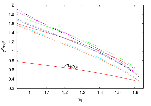
As a last step, we verify if there is a special value of the parameter $\gamma_{q}$ of particular importance. To this end, we have evaluated the $\chi^{2}/\mathrm{ndf}$ of the fit as a function of a given fixed $\gamma_{q}$ within a range $\gamma_{q}\in(0.95,\gamma_{q}^{\mathrm{crit}})$ . This $\chi^{2}$ profile curves, seen in figure 5, all pass $\gamma_{q}=1$ smoothly, therefore $\gamma_{q}=1$ has no special importance for the SHM. However, fits to data in all centralities decrease in $\chi^{2}$ as $\gamma_{q}$ increases, they all point to best fit value of $\gamma_{q}$ near the critical value of Bose–Einstein condensation given by Eq. 7.

The most peripheral bin (70–80%, $N_{\rm part}=15.8$ ) analyzed here requires further discussion as it shows in figure 5 a different behavior and in particular a considerably lower $\chi^{2}$ when $\gamma_{q}\to 1$ . For this peripheral centrality bin the procedure we use to interpolate data of $\Xi$ , $\Omega$ , $\Lambda/\pi$ and K^∗/K assigns a narrow peripheral centrality range to these experimental data points obtained for a much greater centrality domain spanning a participant range which is considerably wider. This can be a problem since within the wider centrality range the experimental results change rapidly with participant number. Therefore, our extrapolation towards the edge of the experimental data centrality range may introduce a fit aberration, here it happens that the created data are less incompatible with equilibrium SHM variants when $\gamma_{q}\to 1$ . We do not believe that there is any issue with result of the fit for $\gamma_{q}\to 1.6$ we discuss in this work. A different approach, in which we recombine the bins rather than to inter-extrapolate was presented in Ref.[37].

II.3 Particle yields

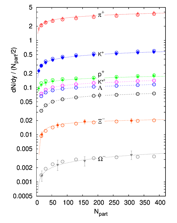
We compare input to the resulting particle yields graphically in figure 6. We fit 13 particles, counting anti-particles, which in the figure cannot be visually distinguished as an independent input or output data, and ratios $\Lambda/\pi$ , K^∗/K and $\phi/$ K. For these ratios, the relevant yield outputs $\Lambda$ , K^∗ and $\phi$ are shown. Direct comparison of the input $\Lambda/\pi$ , K ${}^{*}/$ K and $\phi/$ K ratios to the output is presented in figure 7, note that $\phi/$ K ratio is available as experimental data point in all centrality bins. The fitted output yields are stated also in the top portion of table 2, and ratios are given just below allowing for comparison with the input values.

Table 2: Table of hadron yield output; header of the table defines the centrality bins in three different ways. Top section of the table shows fitted yields

dN/dy

of hadrons entering the fit at LHC2760 obtained in the chemical non-equilibrium SHM. Next below are three ratios that are actually included in the fit (rather than the yields of

\Lambda,

K^0∗,

\phi

), followed by the ratios of hadron yields that can be formed from the stated results, stated here for convenience of the reader. In the two lower sections of the table, there are predicted yields of yet unmeasured hadrons and at the very bottom, we show predicted yields of light anti-nuclei scaled up by factor 1000 (and by

10^{6}

for anti-Helium). Note that yield of matter particles is nearly the same.

Centr.bin	0–20%	0–5%	5–10%	10–20%	20–30%	30–40%	40–50%	50–60%	60–70%	70–80%
$\langle N_{\mathrm{\rm part}}\rangle$	308	382.8	329.7	260.5	186.4	128.9	85.0	52.8	30.0	15.8
$dN_{\rm ch}/dy$	$1312$	$1732$	$1433$	$1075$	$729$	$474$	$294$	$169$	$88.7$	$40.2$
$\pi^{+}$	$525$	$696$	$574$	$431$	$292$	$190$	$118$	$68.0$	$35.8$	$16.4$
$\pi^{-}$	$525$	$696$	$575$	$430$	$292$	$189$	$118$	$68.1$	$35.9$	$16.4$
K⁺	$88.4$	$115$	$96.0$	$71.8$	$49.0$	$31.4$	$19.2$	$10.8$	$5.41$	$2.30$
K^-	$88.1$	$114$	$95.5$	$72.1$	$48.7$	$31.5$	$19.1$	$10.8$	$5.37$	$2.30$
$\mathrm{p}$	$26.5$	$34.9$	$29.0$	$22.0$	$15.1$	$10.1$	$6.45$	$3.82$	$2.08$	$0.982$
$\mathrm{\overline{p}}$	$26.1$	$34.2$	$28.4$	$21.6$	$14.8$	$9.89$	$6.30$	$3.72$	$2.02$	$0.953$
K^0∗	$20.8$	$27.0$	$22.6$	$17.0$	$11.7$	$7.56$	$4.68$	$2.67$	$1.36$	$0.587$
$\phi$	$11.2$	$14.4$	$12.1$	$9.12$	$6.23$	$3.99$	$2.40$	$1.33$	$0.632$	$0.255$
$\Lambda$	$17.2$	$22.3$	$18.6$	$14.2$	$9.73$	$6.43$	$4.00$	$2.31$	$1.18$	$0.520$
$\Xi^{-}$	$3.03$	$3.86$	$3.25$	$2.49$	$1.70$	$1.11$	$0.674$	$0.377$	$0.181$	$0.0745$
$\overline{\Xi}^{+}$	$3.00$	$3.80$	$3.22$	$2.43$	$1.68$	$1.08$	$0.664$	$0.371$	$0.179$	$0.0726$
$\Omega^{-}\,10^{3}$	$529$	$663$	$561$	$435$	$297$	$193$	$115$	$62.6$	$28.5$	$11.0$
$\overline{\Omega}^{+}\,10^{3}$	$527$	$654$	$560$	$421$	$295$	$186$	$114$	$62.1$	$28.4$	$10.7$
$\Lambda/\pi\,10^{3}$	$32.7$	$32.0$	$32.4$	$33.0$	$33.4$	$33.9$	$34.0$	$33.9$	$32.9$	$31.7$
K ${}^{0*}\!/$ K $\,10^{3}$	$236$	$235$	$237$	$236$	$239$	$240$	$245$	$248$	$252$	$255$
$\phi/$ K $\,10^{3}$	$127$	$125$	$126$	$127$	$128$	$127$	$125$	$123$	$117$	$111$
$\phi/\pi^{-}\,10^{3}$	$21.4$	$20.6$	$21.0$	$21.2$	$21.4$	$21.1$	$20.3$	$19.5$	$17.6$	$15.6$
K ${}^{-}/\pi^{-}\,10^{3}$	$168$	$165$	$166$	$167$	$167$	$167$	$162$	$158$	$150$	$141$
p $/\pi^{+}\,10^{3}$	$50.4$	$50.2$	$50.5$	$51.0$	$51.8$	$53.2$	$54.8$	$56.2$	$58.0$	$60.0$
$\Xi/\pi\,10^{3}$	$5.76$	$5.55$	$5.65$	$5.79$	$5.84$	$5.86$	$5.71$	$5.53$	$5.06$	$4.55$
$\Omega/\pi\,10^{3}$	$1.007$	$0.952$	$0.976$	$1.010$	$1.019$	$1.019$	$0.973$	$0.920$	$0.795$	$0.671$
K ${}^{0*}\!/\pi\,10^{3}$	$39.6$	$38.8$	$39.3$	$39.5$	$40.0$	$39.9$	$39.7$	$39.2$	$37.8$	$35.9$
$\mathrm{p/K}$	$0.300$	$0.303$	$0.302$	$0.306$	$0.309$	$0.322$	$0.336$	$0.354$	$0.385$	$0.426$
$\eta$	$61.0$	$79.7$	$66.3$	$49.8$	$33.9$	$21.9$	$13.4$	$7.64$	$3.90$	$1.72$
$\rho(770)^{0}$	$38.9$	$51.3$	$42.5$	$32.1$	$21.9$	$14.5$	$9.14$	$5.35$	$2.87$	$1.34$
$\omega(782)^{0}$	$35.1$	$46.4$	$38.4$	$29.0$	$19.8$	$13.1$	$8.28$	$4.85$	$2.61$	$1.22$
$\Delta(1232)^{++}$	$4.98$	$6.57$	$5.46$	$4.15$	$2.86$	$1.92$	$1.23$	$0.734$	$0.402$	$0.191$
$\Sigma^{*}(1385)^{-}$	$2.08$	$2.70$	$2.26$	$1.72$	$1.18$	$0.785$	$0.492$	$0.284$	$0.146$	$0.065$
$\Lambda^{*}(1520)$	$1.09$	$1.41$	$1.18$	$0.907$	$0.625$	$0.418$	$0.264$	$0.153$	$0.0795$	$0.0355$
$\Xi^{*}(1530)^{-}$	$1.02$	$1.30$	$1.09$	$0.84$	$0.58$	$0.378$	$0.230$	$0.129$	$0.0626$	$0.0258$
${}^{2}\mathrm{\overline{H}}\,10^{3}$	$74.7$	$98.1$	$81.9$	$62.6$	$43.6$	$29.4$	$19.5$	$11.8$	$6.53$	$3.16$
${}^{3}_{\Lambda}\mathrm{\overline{H}}\,10^{3}$	$0.478$	$0.601$	$0.506$	$0.397$	$0.279$	$0.191$	$0.128$	$0.0773$	$0.0415$	$0.0193$
${}^{3}\mathrm{\overline{H}}\,10^{3}$	$1.64$	$2.13$	$1.79$	$1.39$	$0.983$	$0.677$	$0.468$	$0.290$	$0.166$	$0.083$
${}^{3}\mathrm{\overline{He}}\,10^{3}$	$1.64$	$2.14$	$1.79$	$1.39$	$0.986$	$0.679$	$0.469$	$0.291$	$0.166$	$0.083$
${}^{4}\mathrm{\overline{He}}\,10^{6}$	$5.87$	$7.57$	$6.41$	$5.04$	$3.64$	$2.56$	$1.85$	$1.18$	$0.697$	$0.362$

Our fit results appear as open circles in figure 6, at times completely overlaying the input data, full symbols. For the $\Lambda$ , the dotted line guides the eye, since the actual fit is to the ratio $\Lambda/\pi$ shown in figure 7, no absolute $\Lambda$ data are available, in absence of absolute yields, only open circle, i.e., the fitted value, is shown in figure 6. Similar situation arises with $\phi$ and K^∗, where data are not available, but we fit $\phi/$ K and K ${}^{0*}/$ K. One can see that SHM generated results follow closely both the experimental data available, and the interpolation dashed lines for each particle, and that each interpolation curve passes through the experimental data points shown in full symbols, or at worse, the error bars if these are larger than the symbol.

Even so, we note in figure 6, that our interpolation for $\Omega$ shows a slightly different systematic shape (dashed line) compared the fit results (open symbols) or the behavior of the other particles. In other words, we see that other particles ‘predict’ the yield of $\Omega$ that follows the centrality dependence of other particles, while the four data points lead to a centrality distribution that is slightly different. More precise $\Omega$ data will without any doubt offer a resolution to this slight tension in our interpolation/extrapolation. The hadron yields we find are also stated in table 2. Aside from the yields, we show there frequently quoted ratios of particle yields, e.g., we find p $/\pi^{+}\simeq 0.05$ . We will return to discuss this ratio in subsection III.2.

Figure 7 has the largest differences between theory and experiment. In case of the $\Lambda/\pi$ ratio, we see a systematic within error bar under-prediction at all centralities. For K ${}^{*}/$ K, we see within the error bar a different slope of the fit as a function of centrality. The question can be asked if these differences of fit and results indicate some not yet understood physics contents. However, we are within error bars and such data–fit difference must be expected and is allowed given a large data sample and potential for experimental refinement of these two preliminary data sets involving K^∗ and $\Lambda$ . We recall that at RHIC200, K ${}^{*}/$ K ratio was 10–15% smaller and agrees with current ALICE results within the error margin [35]. We also note that we did not yet study how the charmed hadron decay particles influence the fit.

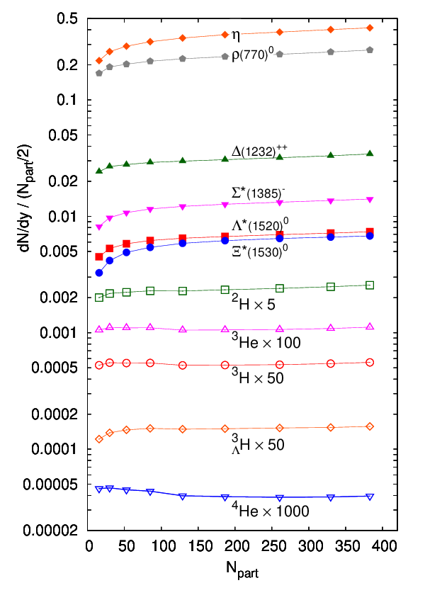
Predictions for the six hadron yields $\eta$ , $\rho^{0}$ , $\Delta(1232)^{++}$ , $\Lambda^{*}(1520)$ , $\Sigma^{*}(1385)^{-}$ , $\Xi^{*}(1530)^{0}$ , are shown in figure 8 as a function of centrality, these results are stated in the lower portion of table 2. We further show five different species of (strange) anti-matter, from anti-deuteron to anti-alpha, including anti-hypertriton, appropriately scaled to fit into display of figure 8. Our predictions of these composite objects should serve as a lower limit of their production rates: fluctuation in the QGP homogeneity at hadronization, and recombinant formation after hadronization may add contributions to the small SHM yield, see here the corresponding RHIC result [36].

III Particle source and its properties

III.1 Statistical parameters

In figure 9, we depict the LHC2760 statistical parameters as a function of collision centrality and compare these LHC2760 results with those we have obtained at RHIC62 [12], shown with open symbols. In all three panels of figure 9, we show parameter errors evaluated by SHAREv2 [4] employing the MINOS minimization routine. One can see that the parameter values for chemical non-equilibrium are defined better than for the case with $\gamma_{q}=1$ .

We present LHC2760 hadronization parameters for the non-equilibrium SHM case also in the top section of table 3. In the top frame figure 9a, we see the particle source volume $dV/dy$ , in the middle frame figure 9b, the chemical freeze-out temperature $T$ , and in the bottom frame figure 9c, the phase space occupancies — the different variants are distinguished by superscripts ‘neq’ (non-equilibrium, that is $\gamma_{q}\neq 1,\gamma_{s}\neq 1$ ) , ‘seq’ (semi-equilibrium, $\gamma_{q}=1,\gamma_{s}\neq 1$ ). and ‘eq’ (equilibrium, $\gamma_{q}=1,\gamma_{s}=1$ ). To compare with the semi-equilibrium SHM variant, we show the ratio $\gamma_{s}^{(\mathrm{neq})}/\gamma_{q}^{(\mathrm{neq})}$ , a ratio which helps to quantify the strangeness to light quark enhancement. This is to be directly compared with the semi-equilibrium strangeness phase space occupancy $\gamma_{s}^{(\mathrm{seq})}$ , given fixed $\gamma_{q}^{(\mathrm{seq})}=1$ .

Table 3: Top section shows chemical non-equilibrium SHM fit parameters

dV/dy

T

\gamma_{q}

\gamma_{s}

and

\chi^{2}_{\rm total}

with ndf (number data less number of parameters) obtained in each centrality bin. For error discussion see text in section III.3. Bottom section presents fireball bulk properties in each bin: energy density

\varepsilon

, pressure

P

, entropy density

\sigma

, strangeness per entropy content

s/S

, entropy at LHC2760 compared to RHIC62,

S_{\mathrm{LHC}}/S_{\mathrm{RHIC}}

and net baryon number per entropy ratio

b/S

. Centrality 0–20% 0–5% 5–10% 10–20% 20–30% 30–40% 40–50% 50–60% 60–70% 70–80% $\langle N_{\mathrm{part}}\rangle$ 308 382.8 329.7 260.5 186.4 128.9 85.0 52.8 30.0 15.8 $dV/dy\,\mathrm{[fm^{3}]}$ $2463\!\pm\!6$ $3304\!\pm\!469$ $2715\!\pm\!81$ $2003\!\pm\!47$ $1337\!\pm\!173$ $853.9\!\pm\!5.9$ $512.2\!\pm\!70.1$ $289.4\!\pm\!5.5$ $149.8\!\pm\!5.0$ $66.9\!\pm\!9.7$ $T\,\mathrm{[MeV]}$ $138.3\!\pm\!0.0$ $138.0\!\pm\!0.0$ $138.1\!\pm\!0.0$ $138.6\!\pm\!0.0$ $139.0\!\pm\!1.7$ $139.9\!\pm\!0.0$ $140.7\!\pm\!1.8$ $141.5\!\pm\!0.0$ $142.3\!\pm\!0.5$ $143.2\!\pm\!2.0$ $\gamma_{q}$ $1.63\!\pm\!0.00$ $1.63\!\pm\!0.00$ $1.63\!\pm\!0.08$ $1.63\!\pm\!0.00$ $1.62\!\pm\!0.08$ $1.62\!\pm\!0.05$ $1.62\!\pm\!0.08$ $1.61\!\pm\!0.00$ $1.61\!\pm\!0.00$ $1.60\!\pm\!0.09$ $\gamma_{s}$ $2.08\!\pm\!0.00$ $2.05\!\pm\!0.17$ $2.06\!\pm\!0.13$ $2.06\!\pm\!0.13$ $2.05\!\pm\!0.16$ $2.00\!\pm\!0.01$ $1.95\!\pm\!0.16$ $1.88\!\pm\!0.05$ $1.75\!\pm\!0.19$ $1.62\!\pm\!0.14$ $\chi^{2}_{\rm total}/{\rm ndf}$ $9.51/9$ $3.87/9$ $3.52/9$ $3.94/9$ $3.35/9$ $4.73/9$ $4.55/9$ $5.65/9$ $6.13/9$ $4.09/9$ $\varepsilon\,\mathrm{[GeV/fm^{3}]}$ $0.462$ $0.453$ $0.457$ $0.467$ $0.476$ $0.487$ $0.505$ $0.516$ $0.521$ $0.527$ $P\,\mathrm{[MeV/fm^{3}]}$ $78.5$ $77.1$ $77.7$ $79.1$ $80.5$ $82.3$ $85.1$ $86.8$ $87.9$ $89.2$ $\sigma\,\mathrm{[fm^{-3}]}$ $3.20$ $3.14$ $3.17$ $3.23$ $3.28$ $3.36$ $3.46$ $3.53$ $3.56$ $3.60$ $s/S$ $0.0299$ $0.0295$ $0.0297$ $0.0297$ $0.0298$ $0.0294$ $0.0290$ $0.0284$ $0.0272$ $0.0257$ $S_{\mathrm{LHC}}/S_{\mathrm{RHIC}}$ $3.07$ $3.23$ $3.10$ $2.93$ $2.75$ $2.56$ $2.33$ $2.06$ $1.74$ $1.27$ $b/S\times 10^{4}$ $1.37$ $2.00$ $2.08$ $2.19$ $2.30$ $2.45$ $2.61$ $2.81$ $3.06$ $3.57$

For the LHC2760 data, the SHM forcing chemical equilibrium of light quarks (i.e., $\gamma_{q}=1$ with either $\gamma_{s}=1$ or $\gamma_{s}\neq 1$ ) have a very similar volume $dV/dy$ , and similar chemical freeze-out $T$ as shown in figure 9a,b, respectively, with nearly overlapping lines for $dV/dy$ . In the non-equilibrium approach, $dV/dy$ is reduced by about 20–25%, and the freeze-out temperature $T$ by 10% compared to the equilibrium SHM variant. Compared to the RHIC62 results [12] (open symbols) the LHC2760 volume $dV/dy$ is up to a factor 4 larger while the LHC hadronization temperature $T$ is 2–5 MeV lower. Thus, given equal number of participants $N_{\mathrm{part}}$ at RHIC62 and LHC2760, the much larger particle multiplicity $dN/dy$ requires in consideration of the universal hadronization condition [37] considerably increased transverse dimension of the fireball at the time of hadronization, which we find within our SHM interpretation of hadron production data. We understand this growth of particle multiplicity (and therefore volume) as being due to a greater transverse fireball expansion, driven by the greater initial energy density formed in LHC2760 heavy ion collision. This corresponds to a greater initial pressure necessary for the matter expansion to the same bulk hadronization conditions as already found at RHIC. The small but systematic decrease of the freeze-out temperature at LHC2760 compared to RHIC62 may be an indication of a greater supercooling caused by the more dynamical LHC expansion.

The freeze-out temperature $T$ at LHC2760 decreases when considering more central collisions, see figure 9b. In the hadronization scenario used in this work, this can be interpreted as being due to a deeper supercooling of the most central and most energetic collision systems. We can extrapolate the freeze-out temperature to $N_{\mathrm{\rm part}}=0$ in the figure to set an upper limit on hadronization temperature at LHC2760, $T_{\mathrm{had}}\to 145\pm 4\,{\rm MeV}$ , applicable to a small (transverse size) fireball. This, then, is the expected hadronization temperature without supercooling. Excluding, in figure 9b, the most peripheral $T$ -fit point for RHIC62, which does not have a good confidence level, we see that $T$ at RHIC62 converges towards the same maximum value as we found at LHC2760, thus confirming the determination of $T_{\mathrm{had}}$ as the common hadronization temperature without supercooling.

We show the phase space occupancies $\gamma_{q},\gamma_{s}$ in figure 9c. We note that the LHC2760 fit produces nearly a constant $\gamma_{q}$ as a function of centrality. However, $\gamma_{s}$ (and respectively $\gamma_{s}/\gamma_{q}$ ) decrease for more peripheral collisions towards unity suggesting that these flavors approach the same level of chemical equilibrium for systems of small transverse size. A similar situation for peripheral collisions was observed for RHIC62. However, at RHIC62, we see a strong centrality dependence of $\gamma_{s}$ and hence $\gamma_{s}/\gamma_{q}$ . This rapid rise of the RHIC62 $\gamma_{s}$ as a function of centrality can be attributed to the buildup of strangeness in QGP formed at RHIC62, which is imaged in the later produced strange hadron yield. Note that, omitting the most peripheral RHIC62 point, the peripheral $\gamma_{q}$ is nearly the same as at LHC2760. The small difference can be attributed to the smaller allowed value of $\gamma_{q}$ for the slightly higher value of $T$ seen at RHIC62.

We have executed all our fits allowing for the presence of the chemical potentials (Eq. 1) characterizing the slight matter–anti-matter asymmetry present at LHC2760. The quality of the fit is not sufficiently improved including effectively one extra parameter ( $\mu_{B}$ , since $\mu_{S}$ is fixed by strangeness conservation) to assure that the unconstrained results for $\mu_{B}$ are convincing. As mentioned in section II.1, we smooth the centrality dependence of $\mu_{B}$ by introducing baryon stopping fraction at mid-rapidity, that is imposing Eq. 5 as an additional data point, a value that we saw a few times in the data without introducing this constraint. This constraint leads to the chemical potentials $\mu_{B}$ and $\mu_{S}$ presented in figure 10, with the baryochemical potential $1\leq\mu_{B}\leq 2.3$ MeV and $\mu_{S}=0.0\pm 0.5\,\mathrm{MeV}$ for all centralities, values an order of magnitude smaller than at RHIC62 and RHIC200. As we can see, even with the constraint, there are two centralities which do not agree with the trend set by the other seven data points.

Data shown in figure 10 are not defined well enough to argue that we see a decrease of baryochemical potential with increasing centrality, since this outcome could be result of the bias we introduced. However, we think that for the most central collisions at LHC2760 there is some indication that $\mu_{B}\simeq 1.5$ MeV. Dashed line in figure 10 indicates the resultant baryon per entropy, $b/S$ , scaled with 5000, these values are also seen in table 3. This is a first estimate of this important result needed for comparison with the conditions prevailing in the big bang early Universe where $b/S\simeq 3.3\times 10^{-11}$ [38].

III.2 p $/\pi$ ratio and chemical (non-)equilibrium

The key difference between the three SHM approaches are the values of $\gamma_{q,s}$ , as seen in figure 9c. In section II.1, we argued that the baryon to meson ratio, e.g., p $/\pi$ , is directly proportional to $\gamma_{q}$ and this can be used to distinguish between the three SHM approaches. This ratio is a big problem for the equilibrium SHM [6]. We wish now to quantify this result within our approach and to show that, within the chemical non-equilibrium SHM, the problem is solved.

For this purpose, we redo all fits but making this ratio more explicit in the data analysis. Specifically, first we evaluate p $/\pi$ ratio based on the yields of p and $\pi$ seen in table 1

\frac{\mathrm{p}}{\pi}\equiv\frac{\mathrm{p}\,\,+\,\,\overline{\mathrm{p}}}{\pi^{-}+\pi^{+}}.

(8)

We estimate the error of the p $/\pi$ ratio by adopting the relative error of p $/\pi$ from [6], that is 6.5%. We include this new data point, p $/\pi$ ratio, in the fit. Note that this increases the relative importance of p and $\pi$ compared to the other particles included in the fit. Open symbols in the figure 11a depict the data and full symbols show the resulting output values obtained when we refit with enlarged data set that includes the p $/\pi$ ratio. There is a minimal change in statistical parameters and physical properties of the fireball which we do not restate. In figure 11b, we show $\chi^{2}_{\rm total}$ .

Even with the increased importance of p $/\pi$ , the chemical non-equilibrium SHM works very well. However, SHM with fixed $\gamma_{q}=1$ have increased difficulties describing this ratio, that is there is systematic 1.5–2 s.d. difference of the fit result and data and the value of $\chi^{2}_{\rm total}$ is large. When compared to the $\chi^{2}_{\rm total}$ obtained without the added p $/\pi$ in figure 2, the non-equilibrium variant shows nearly the same values of $\chi^{2}_{\rm total}$ for all centralities, the p $/\pi$ ratio is a natural outcome of the non-equilibrium approach. On the other hand, SHM approaches with $\gamma_{q}=1$ show additional systematic increase in $\chi^{2}$ by a factor of $\sim 1.3$ –1.5 for all centralities. This means that p $/\pi$ data are in conflict with the hypothesis $\gamma_{q}=1$ . This demonstrates that the hypothesis of chemical equilibrium of light quarks is incompatible with the baryon to meson ratio at LHC2760 and $\gamma_{q}\simeq 1.6$ is needed in order to describe the LHC data. This finding is in agreement with the RHIC200 data [39], where the importance of the p $/\pi$ ratio was noted.

To compare p $/\pi$ ratio with our predictions, recall that the picture of universal hadronization condition with universal hadronization pressure $P=82\pm 5$ MeV has been advanced by our group [11, 40, 37]. For this favored hadronization condition, the p $/\pi$ ratio is predicted in table II of Ref. [41] to be p $/\pi=0.047\pm 0.002$ , which agrees practically exactly with the experimental result shown in figure 11a. The ALICE collaboration [30] considers and discusses the mechanism of chemical equilibrium hadron production followed by post-hadronization interactions [42, 43, 44, 45, 46], specifically proton–antiproton annihilation, in order to justify the small p $/\pi$ ratio, as compared to the result of equilibrium SHM alone. However, the annihilation mechanism was proposed based on preliminary data available in a single centrality bin 0–20%, whereas our work includes more recent and centrality dependent experimental results [30], allowing a far more conclusive study of the annihilation model.

Aside from $\mathrm{p\overline{p}}$ annihilation, there are $\mathrm{p\overline{p}}$ formation events. The significantly larger abundance (and therefore also density) of heavy mesons compared to nucleons, see table 2, implies that mesons can be an effective source of nucleon pairs in reactions such as $\mathrm{p+\overline{p}}\longleftrightarrow\rho+\omega$ and many other relevant reactions, see table II in Ref.[47]. ALICE collaboration notes, that p $/\pi$ ratio modification after annihilation should disappear in most peripheral collisions due to smaller volume. We will now quantify this effect showing how this fade-out of the annihilation effect would work as a function of centrality. We show that given the constant p $/\pi$ ratio in a wide range of centralities, figure 11a, the effect of post-hadronization change of p $/\pi$ ratio must be negligible.

In order to establish the centrality dependence of post-hadronization nucleon yield changing reactions, we evaluate the total number of $\mathrm{p\overline{p}}$ annihilation events. This number is obtained by integrating annihilation rate over history of the post-hadronization matter expansion

N_{\rm annih}=\int dtN_{\mathrm{\overline{p}}}(t)\rho_{\mathrm{p}}(t)\sigma_{\rm annih}v,

(9)

where $v$ is the relative velocity of $\overline{p}$ and $p$ . The three-dimensional dilution of the density can be modeled as

	$\displaystyle\rho_{\mathrm{p}}(t)$	$\displaystyle=\frac{\rho_{\mathrm{p}}^{h}}{(1+\langle v_{\rm flow}\rangle t/\langle L\rangle)^{3}},$		(10)
	$\displaystyle\langle L\rangle$	$\displaystyle\simeq[(dV/dy)/(4\pi/3)]^{1/3},$

where $\langle L\rangle$ is the magnitude of the fireball size, and $\langle v_{\rm flow}\rangle\simeq 0.6$ – $1\,c$ is the velocity of the fireball expansion, in both cases averaged over the fireball complex three dimensional geometry.

The initial density at time of hadronization is obtained from our hadronization study:

\rho_{\mathrm{p}}(t_{h})\equiv\rho_{\mathrm{p}}^{h}\simeq\rho_{\mathrm{\overline{p}}}^{h}\equiv\frac{{dN_{\mathrm{p}}}/dy}{dV/dy}.

(11)

In a wide range of low relative energies, which are relevant here, the event cross section is [48]

\sigma_{\rm event}\equiv\sigma_{\rm annih}v/c\simeq 46\,\mathrm{mb}.

(12)

Neglecting the depletion of nucleons (i.e., $N_{\mathrm{\overline{p}}}(t)\simeq N_{\mathrm{\overline{p}}}^{h}$ ), we find, combining Eq. 9 with Eq. 10, the ratio of annihilated (anti)protons to their total yield ${N_{\rm annih}}/{N_{\mathrm{\overline{p}}}^{h}}$ and proton mean path before it annihilates $L_{\rm event}$ :

\frac{N_{\rm annih}}{N_{\mathrm{\overline{p}}}^{h}}=\frac{\langle L\rangle}{2\langle v_{\rm flow}/c\rangle L_{\rm event}},\qquad L_{\rm event}=\frac{1}{\sigma_{\rm event}\rho_{\mathrm{p}}^{h}}.

(13)

The upper three lines, in figure 12, show $L_{\rm event}$ for the three models of hadronization (equilibrium, semi-equilibrium and non-equilibrium) as a function of centrality. The colored band in figure 12 represents the error originating from the freeze-out temperature $T$ uncertainty (see figure 9). Note that the non-equilibrium model has much smaller parameter errors, so $L_{\rm event}$ is defined more precisely. Since the event reaction cross section for annihilation is well measured and nearly constant, it does not introduce any additional uncertainty to $L_{\rm event}$ . The bottom three lines, in figure 12 (semi-equilibrium and equilibrium lines overlap, since $dV/dy$ is very similar in these two cases), show how the size $\langle L\rangle$ of the system changes as a function of centrality. Especially for peripheral collisions, we see that $\langle L\rangle\ll L_{\rm event}$ . The ratio of both length scales provides a measure of the fraction of protons that can be annihilated.

As seen in figure 12, from central to semi-peripheral ( $N_{\rm part}\simeq 85$ ) collisions, the ratio of both lengths nearly doubles. This means that the annihilation fraction drops in semi-peripheral collisions to about half of the most central value. However, the measured ratio p $/\pi$ is nearly constant over this range, increasing from $0.046\pm 0.003$ to $0.050\pm 0.003$ . We interpret this as experimental evidence that the net effect of $\mathrm{p\overline{p}}$ formation and annihilation is insignificant. Therefore, the annihilation of $\mathrm{p\overline{p}}$ pairs cannot serve as the explanation of the disagreement between the equilibrium SHM and observed small value of p $/\pi$ ratio.

Our estimate of the annihilation effect based on Eq. 13 and the result seen in figure 12 is consistent with the annihilation effect reported in Ref. [42], where detailed balance reactions forming $\mathrm{p\overline{p}}$ were not considered. In this work, p $/\pi$ rises to p $/\pi=0.058$ already in the 20–30% centrality bin ( $N_{\rm part}=185$ ), which is more than 3 s.d. above experimental data (see figure 11a). Another work Ref. [44] addresses directly our scenario of describing the experimental p $/\pi$ ratio and shows that with annihilation the required temperature would be $T=165\pm 5\,\mathrm{MeV}$ while without baryon annihilation a hadronization temperature of $T=145\pm 5\,\mathrm{MeV}$ is required (initial yield from equilibrium SHM). Such models of post-hadronization interactions also predict depletion of $\Xi$ yield and enhancement of $\Omega$ yield [45, 46, 44], which leads to even greater discrepancy between at least one of the multistrange baryons and equilibrium SHM predictions, since these yields as obtained before annihilation are already in general below the experimental data (see figure 1a,c).

We do not see a scenario that would allow equilibrium SHM with hadronic afterburners to remain a viable model which can explain a) the reduction of p $/\pi$ ratio from equilibrium SHM value as a function of centrality, and b) the yields of the multistrange baryons at the same time. On the other hand, the experimental value of p $/\pi$ ratio was predicted [41]. The experimental result, the almost centrality independent p $/\pi$ ratio seen in figure 11 (note that the scale is greatly enhanced) is now successfully fitted within non-equilibrium SHM in this work without any modifications to the model or essential change in model parameter values.

III.3 Fireball bulk properties

In order to obtain the bulk physical properties of the source of hadronic particles, we use exactly the same set of particles and the same assumptions about their properties as we employed in the fit procedure. Therefore, the physical properties we determine are consistent with the particle yields that originated our fit. In other words, we sum the energy, entropy, etc. carried away by the observed particles, adding to this observed yield the contributions due to unobserved particles used in the SHM fit.

The bulk physical properties of the hadronizing fireball, that is energy, pressure, entropy and strangeness per entropy content are shown in the bottom part of table 3 and in figure 13 where shaded domains show our error estimate. Solid symbols are results of the fit, lines guide the eye. In our SHAREv2 fit with MINOS minimization, the largest uncertainty seen in table 3 is the $\gamma_{s}$ and $dV/dy$ error, see figure 9, other statistical bulk properties have relatively insignificant errors. As can be seen in table 3, multi-dimensional fits to data can result in nearly all of the fit error accumulating in the uncertainty of two or even just one parameter. In our fits, we see that the dominant uncertainty is in the volume normalization.

When error is found in a few if not only one parameter, we checked for uncertainty arising within an experimental data stability test. We test how a fit is modified when a small subset of experimental data points is altered arbitrarily but within error. We find that fits comprising input data with such arbitrary modification have in general larger errors distributed among all parameters. The convergence of the intensive parameters (e.g., $T$ ) in our initial fit suggests only a very small statistical error inherent to the data, while the extensive parameters (e.g., $V$ ) show a large error common to particle yield normalization. In this situation, predicted ratios of hadron species should be more precise than their individual errors suggest. This is due to the experimental normalization of particle yields being, as this study indicates, strongly correlated. The presence of not vanishingly small error in $\gamma_{s}$ could be a signal of additional source of strange hadrons, for example charm hadron decays.

All fit errors propagate into the properties seen in figure 13. Since in figure 9 we consider densities, the error in volume does not affect these values. Therefore, by recomputing the properties of the fireball shifting alone the value of $\gamma_{s}$ within one s.d., we obtain a good error evaluation in the measurement of the bulk physical properties shown in figure 13. The point that stands out with very small error is at $N_{\rm part}=130$ . This anomaly is due to accidental appearance of a sharp minimum in the highly non-trivial 7-dimensional parameter space.

We are interested in studying the bulk properties of the source of hadrons in order to test the hypothesis that a QGP fireball was the source of particles observed. For this to be true, we must find appropriate magnitude of bulk properties consistent with lattice results, and at the same time, a variation as a function of centrality that makes good sense. We observe in figure 13 a smooth and slow decrease of energy density $\varepsilon$ (top), entropy density $\sigma$ (middle) and hadronization particle pressure $P$ (bottom) as a function of centrality. This slow systematic decrease of all three quantities is noted in particular comparing to RHIC62 (open symbols), where the properties seem to vary less. This maybe interpreted as an effect of volume expansion at LHC leading to larger supercooling for larger systems.

The local thermal energy density of the bulk is the source of all particles excluding the expansion flow kinetic energy. The value we find is $\varepsilon\simeq 0.50\pm 0.05\,\mathrm{GeV/fm^{3}}$ in the entire centrality range. Nearly the same value is found within the chemical non-equilibrium approach for RHIC62 [12] and RHIC200 [10]. We note that $\varepsilon$ assumes the smallest value for the most central collisions, see table 3 and figure 13. The hadronization pressure $P$ and entropy density $\sigma$ are also decreasing for more central collisions, which is consistent with our reaction picture of expanding and supercooling fireball — the larger system in central collisions exhibits more supercooling reflected by a decrease of hadronization temperature and the above mentioned behavior of bulk properties. The error band is (as for $\varepsilon$ ) based on $\gamma_{s}$ uncertainty.

In the last row of table 3, we show that entropy yield at LHC2760 is more than 3 times greater than obtained at RHIC62. The entropy yield $dS/dy$ as a function of participant number is shown in figure 14, and the notable feature is that the power law parametrization displays a nearly linear dependence at RHIC62 while at LHC2760 a strong additional entropy yield, associated with the faster than linear increase, is seen: $dS/dy\propto N_{\rm part}^{1.184}$ . Most of the entropy is produced in an initial state mechanism which remains to be understood and our finding of the nonlinear entropy growth with $N_{\rm part}$ adds to the entropy production riddle and important observational result.

However, at LHC2760, one expects a component in the entropy count arising from the inclusion of the decay products of heavy charmed hadrons in the hadron yield. This entropy component is different from entropy produced in initial reactions, this is the entropy arising from hard parton collision production of charm, and post-hadronization decay of charmed hadrons. It is unlikely that the non-linearity of the entropy yield is due to this phenomenon as one can easily see that the required charm yield would be very large. We will return, in near future, to this question. The uncertainty of entropy depicted in figure 14 as a shaded band is based alone on $\gamma_{s}$ variation, as was obtained for other physical properties in figure 13. A further error due to variance in $dV/dy$ is shown as a separate error bar. Where it is invisible for the LHC2760, it is hidden in symbol size.

We turn now to study strangeness per entropy $s/S\equiv(ds/dy)/(dS/dy)$ in the source fireball. We are interested in this quantity since both entropy and strangeness yields are preserved in the hadronization process. Therefore, by measuring $s/S$ , we measure the ratio of strange quark abundance to total quark and gluon abundance which determines the source entropy, with a well known proportionality factor. For the presently accepted small strange quark mass $m_{s}(\mu=2{\rm GeV})=95\pm 5$ MeV [49], the predicted value shown in figure 5 of Ref. [50] is $s/S\simeq 0.0305\pm 0.0005$ . Finding this result in our LHC data analysis is necessary in order to maintain the claim that the source of hadrons is a rapidly disintegrating chemically equilibrated QGP fireball.

In the figure 15a, we show the strangeness per entropy $s/S$ in the source fireball. The solid squares are for the LHC2760, and open symbols for RHIC62. We see that $s/S$ saturates at $s/S\simeq 0.030$ at LHC2760, a value reached already for $N_{\rm part}>150$ , thus for a smaller number of participating nucleons than we found at RHIC62, and which value remains constant up to the maximum available $N_{\rm part}$ . This agrees with equilibrated QGP hypothesis and suggests that the source of hadrons was in the same conditions for a wide range of centrality.

This constant $s/S$ value as a function of centrality can be interpreted as an evidence of chemical equilibrium for a QGP source: the strangeness yield normalized to all quark and gluon yield inherent in $S$ can be constant only if dynamical processes find a chemical balance for the differently sized fireballs. The value $s/S=0.03$ is in excellent quantitative agreement with microscopic model of strangeness production and equilibration in QGP [50, 51], adopting latest strange quark mass value. The high QGP strangeness yield oversupplies in hadronization the hadron phase space resulting in $\gamma_{s}\simeq 2$ seen in figure 9. Considering the RHIC results shown in figure 15a, we see a slightly higher $s/S$ saturation limit for most central collisions, though the difference is within the RHIC error band (not shown). It is possible that $s/S$ LHC2760 result is 5–10% diluted due to inadvertent inclusion in the entropy count of the charm decay hadrons. It is also of interest to note that at RHIC62, $s/S$ increases monotonically (discounting the low confidence level most peripheral point) with increasing $N_{\rm part}$ suggesting that the QGP source reaches chemical equilibrium only for most central collisions. At LHC2760 there is such increase for much lower size volume of the collision centrality $N_{\rm part}<150$ .

In figure 15b, we show the thermal energy cost to make a strange quark–anti-quark pair. At LHC2760, the energy cost to make a strange pair is practically constant for the wide range of mid-central to central collisions, which confirms that strangeness in the QGP fireball is in chemical equilibrium at the time of hadronization. The slight increase of the thermal energy cost for small centralities corresponds to the lower yield of strangeness seen in figure 15a. At RHIC62, we see monotonically improving energy efficiency converging to a value slightly below our new LHC2760 result, but well within the error bar at RHIC62 (not shown). The rise of energy cost for smaller systems relates to the fact that a larger and notable fraction of strangeness was produced in first hard collision processes during the initial stages of the collision which for RHIC62 and LHC2760 is resulting in higher energy needed to produce one strange–anti-strange pair.

III.4 Connection to lattice results and related considerations

Elaborate lattice-QCD numerical computations of QGP–hadron transition regime are available today [24, 25], and are comprehensively reviewed in Ref. [26]: the HotQCD collaboration [25] converged for 2+1 flavors towards $T_{c}=154\pm 9$ MeV. The question how low the value of $T_{c}$ can be, remains in current intense discussion, as the latest work of Wuppertal–Budapest collaboration [27] suggests a low $T_{c}\simeq 145$ MeV. For an expanding QGP with supercooling, this can lead to hadronization below $T_{c}\simeq 145$ MeV and near $T=140$ MeV. This is indeed the range of values of $T$ that we find in our chemical non-equilibrium SHM analysis.

A comparison of lattice results with freeze-out conditions is shown in figure 16. The two bands near to the temperature axis display the lattice critical temperature in the range $T_{c}=154\pm 9\,\mathrm{MeV}$ [25] (red online) and $T_{c}=147\pm 5\,\mathrm{MeV}$ [27] (green online). The symbols show the results of hadronization analysis in the $T$ – $\mu_{B}$ plane. We selected here the results for the most central collisions and heaviest nuclei. The solid (blue) circles are SHARE chemical non-equilibrium results obtained by our group, with result presented in this paper included in the LHC domain, and RHIC and SPS results seen, e.g., in [11, 40, 52]. The LHC2760 freeze-out temperature is in our case clearly below the lattice critical temperature $T_{c}$ . As just discussed, this is expected for supercooling followed by sudden hadronization. We show also $\gamma_{q}=1$ results of other groups: GSI [53, 54], Florence [15, 56, 55], THERMUS [57], STAR [58] and ALICE [6]. These results show the chemical freeze-out temperature in numerous cases well above the lattice critical temperature $T_{c}$ , which in essence means that these SHM calculations are incompatible with lattice calculations.

The two recent lattice results, shown in figure 16, challenge the chemical equilibrium hadronization [14] scenario widely used for the past decade, which produces a hadronization temperature above the lattice phase cross-over results. Two conspiring hypotheses were made in Ref. [14]: 1) there is chemical equilibrium in; 2) a long lived hadron gas phase. Both statements were assumptions without theoretical or experimental evidence ‘confirmed’ by fits to data, which had even with the large experimental errors a rather large $\chi^{2}$ and thus a negligible confidence level. Therefore, this model needed additional support. Lattice results showing $T_{c}=173\pm 8$ MeV were often introduced in support of equilibrium-SHM. Such a high $T_{c}$ appears, for example, in figure 10 in Ref. [59], but reading the text, one sees that it applies to the mathematical case of two light quark flavors on discrete space-time. Allowing for strangeness flavor in QGP, the hadronization temperature must decrease. Therefore, already a decade ago $T_{c}=154\pm 8$ MeV was the best estimate for 2+1 flavors, leading to the consensus range $T_{c}=163\pm 15$ MeV before continuum limit. Present day continuum value we estimate to be $T_{c}\simeq 150\pm 7$ MeV combining the two results seen in figure 16.

An important requirement, for the full chemical non-equilibrium hadronization approach, is that in the hadronization process, quark flavor abundances emerge as produced at an earlier and independent stage of fireball evolution. Our analysis relies on hadronization being fast, not allowing a significant modification of the available quark abundances. These quark abundances at LHC in a wide range of centralities and in most central RHIC collisions are near to the QGP chemical equilibrium abundance. In order for the quark yields to remain largely unchanged during hadronization and after, it is necessary that the transformation from QGP to hadrons (hadronization) occurs suddenly and at a relatively low temperature, near to the expected chemical freeze-out point where particle abundances stop evolving. The two pion correlation experimental results favor sudden hadronization, which has been seen in the results for a long time [21]. The sudden hadronization model was required for consistency with these results [22, 23]. It is associated with chemical non-equilibrium SHM analysis of the data [7, 8]. Today, with lattice QCD transition conditions reaching a low $T$ consensus, the only SHM approach that remains valid is the chemical non-equilibrium.

IV Discussion

IV.1 What is new at LHC

The primary difference between RHIC62 and LHC2760 data is a $4$ -times larger transverse volume $dV/dy$ at hadronization, as seen in figure 9a. Increase of volume at LHC compared to RHIC, rather than a change of hadronization temperature, shows a common source of hadrons, a signature of QGP formation. The increased volume is in qualitative agreement with the two pion correlation studies [60]. Given the nearly constant entropy density at hadronization, the growth of volume drives the total entropy yield, which is up to $3.2$ times greater at LHC2760 than at RHIC62.

Other differences of LHC2760 compared to RHIC62 are: 1) An order of magnitude smaller baryochemical potential $\mu_{\rm B}\simeq 1.5\,$ MeV, see figure 10.
2) Phase-space occupancy $\gamma_{q}$ constant as a function of centrality.
3) Earlier saturation of $\gamma_{s}$ as a function of centrality, and thus $\gamma_{s}/\gamma_{q}$ -ratio following the behavior of $\gamma_{s}$ .
For comparison, at RHIC62, we have a fast increase of $\gamma_{s}$ over the entire range of $N_{\rm part}$ , as is shown in figure 9c. The LHC2760 result is interpreted to mean that the QGP fireball is rapidly chemically equilibrated already for small $N_{\rm part}$ , while at RHIC62, we must have a large value of $N_{\rm part}$ , that is a large volume, and thus large lifespan, to achieve full strangeness chemical equilibrium in the QGP fireball. The value $s/S=0.03$ is in excellent qualitative agreement with microscopic model of strangeness production and equilibration in QGP and the associated predictions of the final state yield [50, 51].

As a comparison of our present work with our predictions [41] shows, the yield of strangeness is $\sim 20\%$ below our prior expectations. These were motivated by consideration of a very rapidly diluting QGP fireball, wherein the early strangeness QGP equilibrium is preserved and leads to overabundance, above QGP chemical equilibrium at time of hadronization. Such behavior was indicated given the RHIC results showing a steady rise, see figure 15a for RHIC62. Instead, we find a perfectly equilibrated QGP fireball: the observed value of $s/S\simeq 0.03$ is expected for a chemically equilibrated QGP fireball near hadronization condition. This equilibrium QGP saturated value $s/S=0.03$ is observed for many centralities. Since to obtain our prediction we used $s/S=0.037$ , both the value of $\gamma_{s}$ and yields of Kaons are equally $\sim 20\%$ suppressed compared to expectation [41], and other strange particles as well. How this is possible will be one of the riddles that future data and theoretical modeling will need to address. For us, this strangeness suppression compared to expectation is the most remarkable difference from RHIC data that we have found in this first LHC result analysis.

IV.2 Centrality dependence

Considering the bulk properties of the fireball at hadronization, the most remarkable finding is that there is so little centrality dependence. This means that at LHC2760 the source of hadrons is a hot drop of energy that varies mainly in volume as we vary the collision geometry. This applies to energy density $\varepsilon\simeq 0.50\pm 0.05\,\mathrm{GeV/fm^{3}}$ , hadronization pressure $P$ and entropy density $\sigma$ in the entire centrality range, see table 3 and figure 13. These bulk properties decrease monotonically and slowly and assume the smallest value for the most central collisions, supporting the reaction picture of expanding and supercooling fireball — the larger system supercools a bit more. Recall that the error bands in figure 13 are based on $\gamma_{s}$ uncertainty. The one clear centrality dependence of the fireball we find is the rapid rise and early appearance of the strangeness yield saturation seen in figure 15a.

The chemical freeze-out temperature $T$ decreases by about 3 $\,{\rm MeV}$ at all centralities compared to RHIC62, see middle panel in figure 9 (we do not consider here the most peripheral RHIC62 result which has small confidence level). We believe that this result is related to the need to expand and supercool further the initial energy and entropy rich LHC2760 fireball. The large expanding QGP matter pushes further out, supercooling more and yielding a further reduction in the sudden hadronization temperature. The freeze-out temperature $T$ increases towards more peripheral collisions, see figure 9b, which can be explained by the disappearance of supercooling present for the most central and most energetic collision systems. Considering the behavior of both LHC2760 and RHIC62 for $N_{\rm part}\to 0$ , we obtain $T_{\mathrm{had}}\to 145\pm 4\,{\rm MeV}$ , applicable to hadronization without supercooling. This value is in good agreement with the latest lattice result [27] for transformation temperature from QGP to hadrons.

The value of temperature and its behavior as a function of centrality and heavy ion collision energy suggest that produced hadrons emerge directly from a sudden break-up of quark–gluon plasma. The hadron particle density at this low $T$ is sufficiently low to limit the particle number changing reactions and render these insignificant. $T=145$ – $140$ MeV is at, and below, the expected QGP phase transition. The presence of chemical non-equilibrium at this low $T$ means that hadrons did not evolve into this condition, but must have been produced directly from the deconfined phase. This is consistent with the two pion correlation time-parameter, which suggests that particles are produced at a scale which is sudden compared to the size of the system, as is expected for a supercooled QGP state undergoing, e.g., a filamenting breakup at $T\simeq 140$ MeV, and the result of such dynamics is qualitatively consistent with the features described here [21].

The second to last row in table 3 shows the ratio of entropy at LHC2760 to RHIC62, $S_{\mathrm{LHC}}/S_{\mathrm{RHIC}}$ , within the rapidity interval $-0.5\leq y\leq 0.5$ . The entropy enhancement factor increases monotonically with centrality, from ratio of 1.27 in the most peripheral bin to ratio 3.23 in the most central bin. This increase requires volume dependent additional entropy production mechanisms, which are more effective for the more central, larger $N_{\rm part}$ , collisions. Such an increase can arise from hard parton collision generated jets, which are better quenched in the larger volume of matter, and in addition in abundant charm production, which decays into hadrons and appears as additional hadron multiplicity, i.e., entropy. As long as the additional entropy is generated in early stages of the fireball evolution, this has little impact on SHM method of approach in study of hadronization. For example, the quenching of QCD jets feeds thermal degrees of freedom that can convert a part of its energy into strangeness. However, charm decay is different as it occurs after hadronization. Thus, it needs to be accounted for and/or proved irrelevant. It is possible that charm decay entropy generating mechanism may be the cause of the slight (5%) strangeness $s$ over entropy $S$ dilution at LHC2760 (see figure 15a).

IV.3 What we learn about hadronization at LHC

The full chemical non-equilibrium is introduced by the way of the parameter $\gamma_{q}\neq 1$ . This allows one to describe a situation in which a source of hadrons disintegrates faster than the time necessary to re-equilibrate the yield of light quarks present. The two pion correlation data provide experimental evidence that favors a rapid breakup of QGP with a short time of hadron production [21], and thus favors very fast, or sudden, hadronization [22, 23]. There has been for more than a decade an animated discussion if the parameter $\gamma_{q}$ is actually needed with arguments such as simplicity used to invalidate the full chemical non-equilibrium approach.

We have shown that only the chemical non-equilibrium SHM describes very well all available LHC2760 hadron production data obtained in a wide range of centralities obtained in the rapidity interval $-0.5\leq 0\leq 0.5$ , and the outcome is consistent with lattice QCD results. We successfully fit the data with $\chi^{2}/\mathrm{ndf}<1$ for all centrality bins, and show a smooth systematic behavior as a function of centrality of both, the statistical SHM parameters, see figure 9, and bulk physical properties, see figure 13, that allow a simple and consistent interpretation. SHM is validated at LHC2760 as it describes precisely yields of different particles in a wide range of collision centrality and which span over more than 5 orders of magnitude, see figure 6.

We have shown that it is impossible to fit the ratio p $/\pi=0.046\pm 0.003$ [5, 6] together with the other data, when choosing a SHM with $\gamma_{q}=1$ . However, p $/\pi\simeq 0.05$ is a natural outcome of our chemical non-equilibrium fit where $\gamma_{q}\simeq 1.6$ . This result was predicted [41]: within the chemical non-equilibrium SHM, p $/\pi|_{\rm prediction}=0.047\pm 0.002$ for $P=82\pm 5$ MeV/fm³ is in agreement with experimental result we discuss here, for most central collisions p $/\pi|_{\rm\scriptsize ALICE}=0.046\pm 0.003$ .

We have discussed, in section III.2, the possibility of p $/\pi$ ratio evolving after hadronization, and found this scenario to be highly unlikely considering that experimental ratio p $/\pi$ does not vary in a wide centrality domain. Therefore, the fact that chemical equilibrium SHM variant over-predicts p $/\pi$ and produces a poor $\chi^{2}_{\rm total}$ , see figure 11b, demonstrates that the chemical equilibrium SHM approach (with or without post-hadronization interactions) does not work at LHC2760. Further evidence for the chemical non-equilibrium SHM comes from universality of hadronization at LHC2760 and at RHIC, see subsection III.3 and Ref.[37].

IV.4 Predicting experimental results

Our prediction of hadron yields [41] required as input the charge particle multiplicity $dN_{\rm ch}/dy$ which normalizes the reaction volume $dV/dy$ . Further, we assumed strangeness per entropy content $s/S$ , and the nearly universal hadronization pressure with preferred value $P=82\pm 5$ MeV/fm³. This is accompanied by the strangeness conservation constraint $\langle s-\bar{s}\rangle=0$ and the projectile–target charge to baryon ratio $Q/B=0.4$ and, as baryochemical potential cannot yet be fully defined, an approximate value $\cal O$ (1) MeV. Using this input with a 5% error, we obtain the most compatible values of $dV/dy,\,T,\,\gamma_{q},\,\gamma_{s}$ and chemical potentials, and we can evaluate the particle yields along with fireball properties.

We have redone the predictions for $\sqrt{s_{NN}}=2.76\,\mathrm{TeV}$ case with the tested and released SHAREv2.2 code and find that the pre-release SHARE predictions in [41] were made for $dN_{\rm ch}/dy=2150$ and not for $dN_{\rm ch}/dy=1800$ . Therefore, all absolute hadron yields stated in Ref. [41] are normalized to be $\sim\!20\%$ too large, in addition to the strangeness overcount originating in the assumption $s/S=0.037>0.030$ . The ratios of hadrons with the same strangeness content were correctly predicted.

Applying our prediction method using the updated strangeness value of $s/S=0.030$ and a more precise hadronization pressure estimate $P\simeq 77\pm 4,\mathrm{MeV/fm}^{3}$ results, for $\sqrt{s_{NN}}=2.76\,\mathrm{TeV}$ , in accurate prediction of all hadron particle yields, statistical parameters, and fireball bulk properties, without using as input any individual hadron yield. This validates our approach [41], which can be applied to the forthcoming Pb–Pb collisions at $\sqrt{s_{NN}}=5.5\,\mathrm{TeV}$ or in the RHIC beam energy scan. Noting that the multiplicity of produced hadrons is synonymous to entropy of the fireball, this result means that all hadron yields can be predicted within the framework of chemical non-equilibrium SHM using as input the properties of the bulk matter in the fireball.

IV.5 Conclusions and outlook

We have shown that the non-equilibrium SHM model in the LHC reaction energy range is yielding a very attractive data fit. We have argued that non-equilibrium SHM is today favored by the lattice results, since we must have $T<T_{c}$ , and lattice is moving lower in $T_{c}$ , see $T_{c}=147\pm 5\,\mathrm{MeV}$ [27]. Only the non-equilibrium SHM range $T<145\,\mathrm{MeV}$ remains convincingly compatible. Considering the dynamics of the fireball expansion $\Delta T\equiv T_{c}-T$ is of magnitude where we would like it for supercooling. Moreover, the chemical non-equilibrium SHM is favored by offering simplicity, as it needs no after-burners. Ockham’s razor argument (lex parsimoniae) can be used to conclude that non-equilibrium SHM is a valid precise description of multi-hadron production.

The good fit within the realm of non-equilibrium SHM of all observed particles allows us to predict with some confidence the yields of yet unmeasured hadrons within the chemical non-equilibrium SHM scheme, which are seen in table 2. The question is how stable these yields are when data basis of the fit increases to include new measurement. A small SHM parameter change should be expected also when we refine the theoretical model by adding features, such as inclusion of hadrons from perturbative QCD jets and/or charm hadron decay contribution to hadron yields. We believe that predictions for the primary ‘stable’ hadrons such as $\eta$ are accurate. On the other hand, even the minor changes in SHM parameters can have relatively large effect especially for anti-matter clusters shown in the bottom part of table 2: in the anti-alpha, we have 12 anti-quarks, and a few % error in understanding their primordial yield is raised to 12th power.

It is quite remarkable that despite a change by a factor of 45 in reaction energy, we find for all centralities at both LHC2760 and RHIC62, that the energy density of hadronizing matter is $0.50\pm 0.05$ GeV/fm³, as is seen in figure 13. In fact, the present day data favor a systematic decrease of hadronization pressure $P$ from peripheral towards central collisions as compared to earlier RHIC62 [12], RHIC200 [10] and our preliminary LHC analysis with limited data set [37]. It is possible that the more dynamical expansion of the LHC2760 fireball and deeper supercooling of the fireball are the cause.

We checked that assuming universal hadronization pressure, we could obtain a very good fit to particle data for all centrality LHC2760 data bins. This means that if and when more hadron yield data are available, the decrease in bulk properties with centrality seen in figure 13 could easily disappear. Therefore, the presence of a constant critical hadronization pressure [40] could extend from SPS to LHC. We are investigating this hypothesis, as well as the possibility that another quantity governs universality of hadronization. We hope to return to the matter as soon as we have understood better the final state contributions to hadron yields from charmed hadron decays.

We have shown that the precise hadron yields measured by the ALICE collaboration at LHC2760 have offered a vast new opportunity to explore the properties of the QGP fireball and to understand the dynamics of its evolution and matter production. We are able to quantify the key physical properties at this early stage. With more data becoming available, we expect a significant refinement and improved understanding of both the QGP fireball and mechanisms of matter creation out of the deconfined QGP phase.

IV.6 Update

We have checked that the new results [61, 62] on strange hadron multiplicities which became available at the beginning of the SQM2013 meeting end of July 2013 are fully compatible: the K_S, $\Omega$ , and $\Xi$ are in remarkable agreement with our here presented evaluations and $\Lambda$ yield is as much off as is our fitted preliminary $\Lambda/\pi$ ratio, see figure 7, that is the theoretical $\Lambda$ yield is in general about 1.2 s.d. smaller compared to the final experimental $\Lambda$ yield. Here we note that the presented fits are carried out without taking into account charmed particle decay products, which beyond the generally enhanced overall hadron multiplicity produce a non-negligible number of additional strange baryons.

Acknowledgments

This work has been supported by a grant from the U.S. Department of Energy, DE-FG02-04ER41318, Laboratoire de Physique Théorique et Hautes Energies, LPTHE, at University Paris 6 is supported by CNRS as Unité Mixte de Recherche, UMR7589. JR thanks CERN-PH-TH for the hospitality while most of this work was carried out. JR thanks members of ALICE collaboration, in particular Karel Safarik, Boris Hippolyte and Federico Antinori, for many conversations and clarifications.

Table 4: Enhancement of multi-strange baryon yields per participant pair relative to p–p collisions, p–p yields and calculated yields in Pb–Pb, which we use as input to our interpolation as a function of

N_{\rm part}

Particle	Ref.	Centr.	$\langle N_{\rm part}\rangle$	p–p data $(dN/dy)_{\mathrm{pp}}$ and enhancement $E$	$(dN/dy)_{\mathrm{PbPb}}=E\,0.8\,(dN/dy)_{\mathrm{pp}}(\langle N_{\rm part}\rangle/2)$
$\Xi^{-}$	[34]	p–p	2	$(8.0\pm 0.7)\times 10^{-3}$
		60–90%	17.6	$E=1.58\pm 0.18$	$0.090\pm 0.010$
		40–60%	68.8	$E=2.48\pm 0.26$	$0.55\pm 0.06$
	[32]	20–40%	157	$E=2.95\pm 0.32$	$1.51\pm 0.17$
		0–20%	308	$E=3.08\pm 0.33$	$3.08\pm 0.33$
$\overline{\Xi}^{+}$	[34]	p–p	2	$(7.8\pm 0.7)\times 10^{-3}$
		60–90%	17.6	$E=1.57\pm 0.19$	$0.087\pm 0.011$
		40–60%	68.8	$E=2.56\pm 0.26$	$0.56\pm 0.06$
	[32]	20–40%	157	$E=3.20\pm 0.35$	$1.59\pm 0.17$
		0–20%	308	$E=3.00\pm 0.32$	$2.91\pm 0.32$
$\Omega^{-}$	[34]	p–p	2	$(0.67\pm 0.08)\times 10^{-3}$
$\overline{\Omega}^{+}$	[34]	p–p	2	$(0.68\pm 0.08)\times 10^{-3}$	$\Omega^{-}$	$\overline{\Omega}^{+}$
(Ω - + $\overline{\Omega}$ + ) 2		60–90%	17.6	$E=2.56\pm 0.53$	$0.012\pm 0.003$	$0.012\pm 0.003$
	[32]	40–60%	68.8	$E=4.57\pm 0.79$	$0.08\pm 0.02$	$0.08\pm 0.02$
		20–40%	157	$E=5.23\pm 0.95$	$0.22\pm 0.05$	$0.21\pm 0.04$
		0–20%	308	$E=6.97\pm 1.27$	$0.57\pm 0.12$	$0.56\pm 0.12$

Appendix A Data rebinning

Rebinning multi strange hadron yields

Since there is no literature stating explicitly the yields of $\Xi$ and $\Omega$ in Pb–Pb collisions, we proceed to obtain these results by unfolding the preliminary enhancement data. We combine the yield of $\Xi$ and $\Omega$ produced in p–p collisions at 7 TeV [34] stated in table 4 and labeled ‘pp’ in the third column therein, with the ‘preliminary’ enhancement $E$ relative to p–p and normalized to a pair of participating nucleons shown in Ref. [31] and which we also show in the fifth column of table 4. We generate the first data point for the centrality bin 0–20% by averaging the number of participants in the centrality bins from 0 to 20% shown in table 1 of Ref. [29]. We reduce the yields of both $\Xi$ and $\Omega$ by a constant factor of 0.8 in order to compensate for the difference in collision energy $\sqrt{s}=7\,\mathrm{TeV}$ in p–p collisions and $\sqrt{s_{NN}}=2.76\,\mathrm{TeV}$ in Pb–Pb. We obtained the magnitude of this energy correction factor by comparing with the actual yield for the 0–20% centrality bin given in Ref. [28]. To disentangle the combined yield of $\Omega+\overline{\Omega}$ , we use the separated $\Omega$ and $\overline{\Omega}$ yields from p–p collisions [34], see table 4.

We use the relative errors of the enhancements to estimate the errors of the multi strange baryon yields, that is $\sim\!11\%$ for $\Xi$ and $\sim\!20\%$ for $\Omega$ . Our adopted $\Omega$ error is larger by $\sim\!3\%$ than the error of its yield in 0–20% centrality bin [28]. We adopted this slightly increased error to account for procedure which lead us to estimate the yield of $\Omega$ , $\overline{\Omega}$ based in part on $\Omega+\overline{\Omega}$ yield. The mathematical operations leading to the yields, the yields and widths we use are stated in self-explanatory fashion in table 4.

To account for the different centrality bins for multi strange baryons as compared to $\pi$ , K, p and $\phi/K$ , we express the centrality bins in terms of average number of participants according to [29] and then interpolate every particle yield $dN/dy$ available as a function of ${N_{\mathrm{\rm part}}}$ with a power law

\frac{dN\left({N_{\mathrm{\rm part}}}\right)}{dy}=a\,{N}_{\mathrm{\rm part}}^{b}+c,

(14)

where $a,b$ and $c$ are free parameters. The form of the function has no immediate physical motivation, it serves well the purpose of unifying the data across incompatible centrality bins. This method enables us to evaluate the invariant yields for any given ${N_{\mathrm{\rm part}}}$ , i.e., arbitrary centrality and thus enables us to include the multi-strange baryon yields in this analysis. Interpolation parameters together with $\chi^{2}$ of each particle interpolation are summarized in table 5. For completeness, and potential future use, we present also the parametrization of $\pi^{\pm}$ , K^± and p^± which do not require rebinning. Small values of $\chi^{2}$ /ndf show that our description is accurate in the given interval of ${N_{\mathrm{\rm part}}}$ . Interpolation curves are depicted with dashed lines in figure 6 for particle yields.

Table 5: Interpolation parameters of particle yields as defined in Eq. 14.

Particle	a	b	c	$\chi^{2}/{\rm ndf}$
$\pi^{+}$	$0.725\phantom{22}$	$1.160$	${-}0.890\phantom{1}$	$0.30/7$
$\pi^{-}$	$0.724\phantom{22}$	$1.160$	${-}0.864\phantom{1}$	$0.22/7$
K⁺	$0.0935\phantom{2}$	$1.187$	${-}0.174$	$0.07/7$
K^-	$0.0927\phantom{2}$	$1.188$	${-}0.158$	$0.06/7$
$\mathrm{p}$	$0.0432\phantom{2}$	$1.116$	${-}0.047$	$0.32/7$
$\mathrm{\overline{p}}$	$0.0502\phantom{2}$	$1.089$	${-}0.088$	$0.26/7$
$\Xi^{-}$	$0.00552$	$1.108$	$-0.043$	$0.12/1$
$\overline{\Xi}^{+}$	$0.00762$	$1.049$	$-0.067$	$0.70/1$
$\Omega^{-}$	$0.000286$	$1.324$	$-0.0006$	$0.40/1$
$\overline{\Omega}^{+}$	$0.000309$	$1.308$	$-0.0011$	$0.21/1$
K ${}^{*0}/$ K	see text for details			$0.032/1$
$\Lambda/\pi$	see text for details			$0.0054/1$

Rebinning K ${}^{0*}/$ K^-, $\Lambda/\pi$ hadron ratios

We include particle ratios K ${}^{0*}/$ K^-, $\phi/$ K^- and $\Lambda/\pi\equiv 2\Lambda/(\pi^{-}+\pi^{+})$ [31]. This adds $\Lambda$ , K^∗0 and $\phi$ into our data set. Since in some ratios certain systematic uncertainties of individual yields cancel out, introduction of ratios is reducing the overall error of the global fit. The ratio $\phi/$ K has an experimental data point in each centrality bin we analyze, removing the need for interpolation or rebinning. Thus the following only addresses K ${}^{0*}/$ K^-, and $\Lambda/\pi$ .

Table 6: Experimentally measured ratios used as input to our interpolation as a function of

N_{\rm part}

Ratio	Ref.	Centr.	$\langle N_{\rm part}\rangle$	Experimental ratio
K ${}^{*0}/$ K^-		60–80%	22.6	$0.333\pm 0.084$
	[31]	40–60%	68.8	$0.285\pm 0.061$
		20–40%	157	$0.245\pm 0.066$
		0–20%	308	$0.194\pm 0.051$
2Λ (π - +π + )		60–80%	22.6	$0.0355\pm 0.0041$
		40–60%	68.8	$0.0371\pm 0.0042$
	[31]	20–40%	157	$0.0365\pm 0.0042$
		10–20%	261	$0.0355\pm 0.0041$
		0–10%	357	$0.0336\pm 0.0040$

There are four, resp. five, data points for K ${}^{*}/$ K , resp. $\Lambda/\pi$ , which we present in table 6. We describe K ${}^{*}/$ K dependence on ${N_{\mathrm{part}}}$ with a power law

\frac{{\rm K}^{*}}{{\rm K}}=f\left({N_{\mathrm{part}}}\right)=16.23({N}_{\mathrm{part}}^{-0.0034}-1)+0.512,

(15)

with total $\chi^{2}/\mathrm{ndf}=0.032/1$ . Systematic behavior of $\Lambda/\pi$ as a function of centrality is qualitatively different from K ${}^{*}/$ K, see figure 7, a power law is not sufficient to properly describe the data. We use a sum of two power laws in the following form

	$\displaystyle\frac{\Lambda}{\pi}$	$\displaystyle=f\left({N_{\mathrm{part}}}\right)$
		$\displaystyle=-6.79\times 10^{-5}\,{N}_{\mathrm{part}}^{0.848}-2\,{N}_{\mathrm{part}}^{-0.00135}+2.03\,,$		(16)

with $\chi^{2}/\mathrm{ndf}=0.0054/1$ . In these two cases, the form of the ratio functions has no immediate physical meaning, it is invented in order to provide an accurate empirical description; note that the bottom of the table 5 presents the fit quality of these two ratios.

Interpolation curves are depicted with dashed lines, in figure 7, for K^∗/K and $\Lambda/\pi$ ratios. To assign an error to the interpolated data points, we take the average nearby experimental error for the given particle yield or ratio. However, by extrapolating the K ${}^{*}/$ K ratio to ${N_{\mathrm{part}}}=382$ , we introduce systematic error due to our choice of the functional form of Eq. 15. To account for this effect, we multiply the error of K ${}^{*}/$ K by $2$ (resp. $1.5$ ) in the most (resp. second to most) central bin we analyze as indicated by the shaded area in figure 7. As seen in figure 6, we also extrapolate $\Omega,\Xi$ , but we do not believe that this adds to the already significant error, considering that our power law interpolation functions describe other hadron yields up to $N_{\rm part}=382$ .

References

[1] P. Bozek and I. Wyskiel-Piekarska, Phys. Rev. C 85, 064915 (2012).
[2] M. Rybczynski, W. Florkowski and W. Broniowski, Phys. Rev. C 85, 054907 (2012)
[3] W. Broniowski and W. Florkowski, Phys. Rev. Lett. 87, 272302 (2001)
[4] G. Torrieri, S. Steinke, W. Broniowski, W. Florkowski, J. Letessier, J. Rafelski, Comput. Phys. Commun. 167, 229-251 (2005). and
G. Torrieri, S. Jeon, J. Letessier, J. Rafelski, Comput. Phys. Commun. 175, 635-649 (2006).
[5] B. Abelev [ALICE Collaboration], arXiv:1209.3285 [nucl-ex].
[6] B. Abelev et al. [ALICE Collaboration], Phys. Rev. Lett. 109 (2012) 252301.
[7] J. Letessier and J. Rafelski, Phys. Rev. C 59, 947 (1999).
[8] J. Letessier and J. Rafelski, Int. J. Mod. Phys. E 9, 107 (2000), and J. Rafelski and J. Letessier, “Hadrons from Pb Pb collisions at 158-GeV/A,” nucl-th/9903018 (unpublished).
[9] J. Letessier and J. Rafelski, Camb. Monogr. Part. Phys. Nucl. Phys. Cosmol. 18, 1 (2002).
[10] J. Rafelski, J. Letessier and G. Torrieri, Phys. Rev. C 72, 024905 (2005)
[11] J. Letessier and J. Rafelski, Eur. Phys. J. A 35, 221 (2008).
[12] M. Petran, J. Letessier, V. Petracek and J. Rafelski, Acta Phys. Polon. Supp. 5, 255 (2012).
[13] F. Becattini, M. Bleicher, T. Kollegger, M. Mitrovski, T. Schuster and R. Stock, Phys. Rev. C 85, 044921 (2012).
[14] P. Braun-Munzinger, D. Magestro, K. Redlich and J. Stachel, Phys. Lett. B 518, 41 (2001).
[15] F. Becattini, P. Castorina, A. Milov and H. Satz, Eur. Phys. J. C 66, 377 (2010).
[16] F. Becattini, J. Manninen and M. Gazdzicki, Phys. Rev. C 73, 044905 (2006).
[17] P. Braun-Munzinger, K. Redlich and J. Stachel, In R.C. Hwa, and Xin-Nian Wang (eds.) “Quark gluon plasma 3” pp 491-599 (World Scientific 2004).
[18] A. Andronic et al. Nucl. Phys. A 837, 65 (2010).
[19] J. Rafelski, Phys. Lett. B 262, 333 (1991).
[20] J. Rafelski, J. Letessier and A. Tounsi, Acta Phys. Polon. B 27, 1037 (1996).
[21] L. P. Csernai, M. I. Gorenstein, L. L. Jenkovszky, I. Lovas and V. K. Magas, Phys. Lett. B 551, 121 (2003).
[22] L. P. Csernai and I. N. Mishustin, Phys. Rev. Lett. 74, 5005 (1995).
[23] J. Rafelski and J. Letessier, Phys. Rev. Lett. 85, 4695 (2000).
[24] G. Endrodi, Z. Fodor, S. D. Katz and K. K. Szabo, JHEP 1104, 001 (2011).
[25] A. Bazavov et al. Phys. Rev. D 85, 054503 (2012).
[26] O. Philipsen, Prog. Part. Nucl. Phys. 70, 55 (2013).
[27] S. Borsanyi, Nucl. Phys. A904-905 2013, 270c (2013), and Presentation at 23rd International Conference on Ultrarelativistic Nucleus-Nucleus Collisions (QM 2012), August 13-18, 2012, Washington, DC, USA.
[28] M. Ivanov [ALICE Collaboration], Nucl. Phys. A 904-905, 162c (2013). and presentation by Marian Ivanov at 23rd International Conference on Ultrarelativistic Nucleus-Nucleus Collisions (QM 2012), August 13-18, 2012, Washington, DC, USA.
[29] B. Abelev et al. [ ALICE Collaboration], arXiv:1301.4361 [nucl-ex].
[30] B. Abelev et al. [ ALICE Collaboration], arXiv:1303.0737 [hep-ex].
[31] S. Singha [ALICE Collaboration], Nucl. Phys. A 904-905, 539c (2013).
[32] D. D. Chinellato [ALICE Collaboration], arXiv:1211.7298 [hep-ex].
[33] A. G. Knospe [ALICE Collaboration], J. Phys. Conf. Ser. 420, 012018 (2013).
[34] B. Abelev et al. [A Large Ion Collider Experiment Collaboration], Phys. Lett. B 712, 309 (2012).
[35] M. M. Aggarwal et al. [STAR Collaboration], Phys. Rev. C 84, 034909 (2011) [arXiv:1006.1961 [nucl-ex]].
[36] B. I. Abelev [STAR Collaboration], Science 328, 58 (2010).
[37] M. Petran and J. Rafelski, arXiv:1303.0913 [hep-ph], Phys. Rev. C (rapid communications) in press.
[38] M. J. Fromerth, I. Kuznetsova, L. Labun, J. Letessier and J. Rafelski, Acta Phys. Polon. B 43 (2012) 12, 2261
[39] H. Z. Huang and J. Rafelski, AIP Conf. Proc. 756, 210 (2005).
[40] J. Rafelski and J. Letessier, J. Phys. G G 36, 064017 (2009).
[41] J. Rafelski and J. Letessier, Phys. Rev. C 83, 054909 (2011).
[42] I. A. Karpenko, Y. .M. Sinyukov and K. Werner, Phys. Rev. C 87, 024914 (2013).
[43] R. Rapp and E. V. Shuryak, Phys. Rev. Lett. 86, 2980 (2001)
[44] Y. Pan and S. Pratt, arXiv:1210.1577 [nucl-th].
[45] F. Becattini, M. Bleicher, T. Kollegger, T. Schuster, J. Steinheimer and R. Stock, arXiv:1212.2431 [nucl-th].
[46] J. Steinheimer, J. Aichelin and M. Bleicher, Phys. Rev. Lett. 110, 042501 (2013)
[47] C. Amsler, Rev. Mod. Phys. 70, 1293 (1998).
[48] W. Brueckner, et al. , Zeitschrift für Physik A Atomic Nuclei, 335, 2 (1990), 217-229
[49] J. Beringer et al. [Particle Data Group Collaboration], Phys. Rev. D 86, 010001 (2012).
[50] I. Kuznetsova and J. Rafelski, Eur. Phys. J. C 51, 113 (2007)
[51] J. Letessier and J. Rafelski, Phys. Rev. C 75, 014905 (2007)
[52] J. Rafelski and J. Letessier, PoS CONFINEMENT 8, 111 (2008).
[53] P. Braun-Munzinger, J. Stachel, J. P. Wessels and N. Xu, Phys. Lett. B 344 (1995) 43.
[54] A. Andronic, P. Braun-Munzinger and J. Stachel, Nucl. Phys. A 772, 167 (2006).
[55] F. Becattini, M. Gazdzicki, A. Keranen, J. Manninen and R. Stock, Phys. Rev. C 69, 024905 (2004).
[56] J. Manninen and F. Becattini, Phys. Rev. C 78, 054901 (2008).
[57] J. Cleymans, H. Oeschler, K. Redlich and S. Wheaton, Phys. Rev. C 73, 034905 (2006).
[58] B. I. Abelev et al. [STAR Collaboration], Phys. Rev. C 79, 034909 (2009).
[59] P. de Forcrand and O. Philipsen, Nucl. Phys. B 642, 290 (2002).
[60] K. Aamodt et al. [ALICE Collaboration], Phys. Lett. B 696, 328 (2011).
[61] B. Abelev et al. [ALICE Collaboration], arXiv:1307.5530 [nucl-ex].
[62] B. B. ABELEV et al. [ ALICE Collaboration], arXiv:1307.5543 [nucl-ex].

Hadron production and QGP Hadronization in Pb–Pb collisions at sN​N=2.76\sqrt{s_{NN}}=2.76 TeV