Classification of topological insulators and superconductors in the presence of reflection symmetry
Abstract
We discuss a topological classification of insulators and superconductors in the presence of both (non-spatial) discrete symmetries in the Altland-Zirnbauer classification and spatial reflection symmetry in any spatial dimensions. By using the structure of bulk Dirac Hamiltonians of minimal matrix dimensions and explicit constructions of topological invariants, we provide the complete classification, which still has the same dimensional periodicities with the original Altland-Zirnbauer classification. The classification of reflection-symmetry-protected topological insulators and superconductors depends crucially on the way reflection symmetry operation is realized. When a boundary is introduced, which is reflected into itself, these non-trivial topological insulators and superconductors support gapless modes localized at the boundary.
pacs
72.10.-d,73.21.-b,73.50.FqI Introduction
Topological insulators and superconductors are symmetry preserving fermionic systems with a bulk energy gap[1, 2]. Relevant symmetry conditions that are necessary to define these symmetry protected topological states can be divided into two categories: non-spatial symmetries and spatial symmetries. The Hamiltonians of non-spatial symmetric systems may possess time reversal symmetry (TRS), particle-hole symmetry (PHS), or chiral symmetry. They have gapless boundary states that are topologically protected and are related to physical quantities, such as the Hall conductivity. The subject started with the recognition by Kane and Mele [3, 4] that by incorporating a spin-orbit coupling in the tight-binding model for graphene, the system will become what is now known as a 2D topological insulator with time reversal symmetry (TRS), as well as the theoretical prediction[5] and experimental observation[6] of such topological states in the HgTe/CdTe quantum well. After that, three-dimensional (3D) topological insulators were predicted [7, 8, 9] and observed;[10, 11, 12, 13] the identification of 3He-B as a topological superconductor was realized.[14, 15, 16, 17] It turns out that those topological insulators and superconductors are just a part of a larger scheme — a complete classification of topological insulators and superconductors has been developed with a unified periodic table [18, 19, 20].
Topological phases protected by these non-spatial discrete symmetries are stable against spatially homogeneous as well as inhomogeneous deformations. In addition, the protected boundary modes (edge, surface, etc) that appear at the boundary of topological phases in the periodic table are completely immune to disorder; for arbitrary strong disorder, as far as the bulk topological character is not altered in the bulk through a phase transition, the boundary can never be Anderson-localized.[18]
With a set of discrete spatial symmetries, a topological distinction among gapped phases (i.e., “symmetry protected topological phase”) can arise as well. One example is inversion symmetry protected topological insulators[21, 22, 23] where inversion symmetry is defined as the invariance of the system under the sign flip of the spatial coordinate , where is the spatial coordinates in spatial dimensions, (for lattice systems, labels a site on a -dimensional lattice). Unlike the case of non-spatial discrete symmetries, for topological phases protected by a set of spatial symmetries, non-trivial bulk topology is not necessarily accompanied by a gapless boundary mode, as the boundary might break the spatial symmetries in question. The implications of certain specific point group symmetries on the topological distinction of ground states has been also discussed.[24, 25, 26, 27] More importantly, Hsieh et al.[28] predicted that one of such spatial symmetric insulators can be realized in the Pb1-xSnxTe material class, and this prediction was experimentally verified by ARPES.[29]
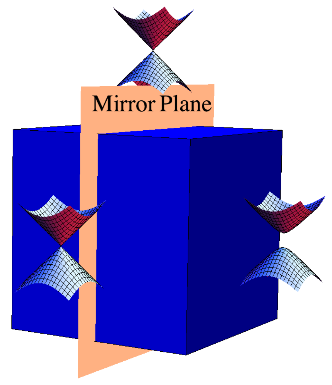
In this paper, we discuss the implication of a reflection (or mirror) symmetry in one spatial direction: it is an invariance of the system under the sign flip of, say, the first component of Cartesian coordinates, . (For an earlier study of this subject, see Ref. 30.) While an inversion symmetry singles out a special point, reflection symmetry singles out a special -dimensional plane ( in the this case). As a consequence, when we terminate the system with a -dimensional boundary (plane) which is orthogonal to the reflection plane (), the boundary with constant () is reflection symmetric under . Reflection symmetry is arguably the simplest spatial symmetry of a system for which certain boundaries can respect the spatial symmetry in question. This boundary property is an important distinction from the inversion symmetric topological phases, for which a plane boundary to the system alone does not inherit the spatial symmetry (inversion symmetry) in the bulk. (A pair of boundaries can be inversion symmetric to each other, though). With the special choice of the boundary above, we will argue that for topologically non-trivial phases protected by reflection there is a stable boundary mode, in the manner similar to topologically phases protected by non-spatial discrete symmetries. The correspondence still holds between the non-trivial bulk topology and the gapless boundary modes when the boundary that reflects to itself is chosen as shown in Figure 1.
Although topological insulators and superconductors protected by non-spatial or spatial symmetries have been studied separately, their recognition does not directly provide a complete classification of topological systems in the presence of both non-spatial and spatial discrete symmetries. Therefore, we will consider the topological classification of reflection symmetric systems with a subset of the three non-spatial symmetries: TRS, PHS, and chiral symmetry. We found the topological classification depends not only on the set of symmetries which are respected but also on the way how reflection symmetry is realized, i.e., algebraic relations satisfied among reflection and other non-spatial discrete symmetries when they exist. Our result of the classification of reflection symmetric systems is summarized in Table 1. The algebraic relations among reflection and non-spatial symmetry operations are denoted by and in Table 1.
Non-trivial topological states displayed in Table 1 are characterized by a topological invariant of integer () or type. For example, the entries in Table 1 marked by indicate the presence of topologically protected states by a topological invariant defined on mirror invariant planes in the Brillouin zone (“mirror topological invariant”). These topological states include 3D topological insulators protected by the “mirror Chern number” discussed in Ref. 30, and 2D topological superconductors with TRS and reflection symmetry (class DIII ) discussed in Ref. 31, which are characterized by reflection winding numbers in the 1D mirror lines. We will generalize those mirror numbers to any spatial dimensions and relevant symmetry classes. Furthermore, we will show that some systems are protected by the topological number and the mirror Chern number simultaneously; the larger one of these two numbers gives a new integral topological invariant (denoted by in Table 1). In other cases, the topolgoical insulators and superconductors in the original periodic table turn out to be invariant under reflection. If this is the case, the same topological invariant also characterizes the non-trivial topology of reflection-symmetric topological insulators and superconductors. These cases are indicated by “0”, , and in Table 1. In short, we claim that the reflection-symmetric topological states are characterized by one of the topological invariants, ‘’, , , , and .
In this manuscript, we use “the minimal Dirac Hamiltonian method” to characterize the AZ symmetry classes with reflection symmetry. Without reflection symmetry the topological classification (Table 2) of the AZ symmetry classes can be studied by Anderson localization,[18] K-theory,[19] and minimal Dirac Hamiltonians.[32, 33] The minimal Dirac Hamiltonian method provides a direct way to produce the original classification (Table 2). In this method, we first write down a bulk Dirac Hamiltonian preserving system’s symmetries in the minimal matrix dimension. The topological class of the system is determined by the existence of a symmetry preserving extra mass term (SPEMT), which keeps the system in the same topological phase during the continuous deformation. If this term exists in the minimal Dirac Hamiltonian, this phase is characterized by ‘0’ topological invariant. If not, we consider a bigger system including two minimal Dirac Hamiltonians. The presence of a SPEMT in this system of the two copies implies topological invariant character. Otherwise, the absence of a SPEMT implies character. When classifying reflection symmetry topological insulators and superconductors, we study the existence of a SPEMT in Dirac Hamiltonians to determine topological characters. Complementary to the minimal Dirac Hamiltonian method, we also look for topological invariants ( and ) in the presence of reflection symmetry to determine bulk topology. The classification of bulk topology in terms of topological invariants is fully consistent with the minimal Dirac Hamiltonian method.
Topological insulators might have topological invariants of strong and weak indices.[34] In the original classification table[19, 18] for a -dimensional system, the strong index is the topological invariant in dimensions and the weak indices are captured by the strong indices in the dimensions less than . However, the complications arise when the weak indices are considered in the classification of reflection symmetric systems. The reason is that the weak indices may not be described by the strong indices in the dimensions less than in the reflection classification table. Moreover, the weak indices might depend on spatial directions. That is, in different directions the weak indices are different because reflection symmetry operation only flips one direction. In this manuscript, we shall focus on only the strong indices of the classification.
To name a few physically interesting topological systems in Table 1, in symmetry class AII in three dimensions, with reflection symmetry specified by , there are topological insulators protected by the invariant. These are nothing but the topological insulator that was proposed by Hsieh et al.[28] and observed by Xu et al.[29] in the Pb1-xSnxTe material class. It is the first experimental realization of crystalline topological insulators. This particular reflection symmetric topological insulator continues to be topologically non-trivial even in the absence of TRS, as indicated by “” in symmetry class A in three dimensions in Table 1. Table 1 also includes topological superconductors protected by reflection symmetry, such as with TRS and reflection symmetry 2D topological superconductors (class DIII ),[31] which are classified by an integral-valued topological invariant. For symmetry class D in two dimensions, which hosts T-breaking topological superconductors in the absence of reflection symmetry, there is a reflection symmetric topological superconductor characterized by a topological invariant. Other examples will also be discussed in Sec. VI.
The manuscript is organized as follows: in Sec. II, we provide the background knowledge of reflection symmetry in band theory, and in particular, describe how we distinguish different realizations of reflection symmetry operation in the presence of other non-spatial discrete symmetries. In Sec. III, we review the connection between the minimal bulk Dirac Hamiltonians and the topology possessing ‘’, and topological invariants in the Altland-Zirnbauer(AZ) symmetry classes without reflection symmetry. Moreover, by considering reflection-symmetric Dirac Hamiltonians we show the correspondence between gapless boundary states and bulk topology. In Sec. IV, we consider the two kinds of the classifications: the reflection symmetry operator commutes with all of the non-spatial discrete symmetries and anticommutes with TRS and PHS operators. In Sec. V, we classify the remaining of the AZ symmetry classes possessing TRS and PHS under the condition that one of these symmetry operators commutes with the reflection symmetry operator and the other anticommutes with the reflection symmetry operator. In Sec. VI, the concrete examples for topological insulators/superconductors protected by reflection symmetry are provided.
| AZ Class | T | C | S | operator | MSC | ||||||||
|---|---|---|---|---|---|---|---|---|---|---|---|---|---|
| AIII | 0 | 0 | 1 | AIII2 | 0 | 0 | 0 | 0 | |||||
| A | 0 | 0 | 0 | 0 | |||||||||
| A | 0 | 0 | 0 | A2 | 0 | 0 | 0 | 0 | |||||
| AI | + | 0 | 0 | 33 3 Spinless systems | AI2 | 0 | 0 | 0 | 0 | ||||
| A | 0 | 0 | 0 | 0 | 0 | ||||||||
| BDI | + | + | 1 | 33 3 Spinless systems | BDI2 | 0 | 0 | 0 | 0 | ||||
| AIII | 0 | 0 | 0 | 0 | 0 | ||||||||
| AI | 0 | 0 | 0 | ||||||||||
| D | 0 | 0 | |||||||||||
| D | 0 | + | 0 | 33 3 Spinless systems | D2 | 0 | 0 | 0 | 0 | ||||
| 44 4 Spin- systems | A | 0 | 0 | 0 | 0 | 0 | |||||||
| DIII | - | + | 1 | DIII2 | 0 | 0 | 0 | 0 | |||||
| 44 4 Spin- systems | AIII | 0 | 0 | 0 | 0 | 0 | |||||||
| AII | 0 | 0 | 0 | ||||||||||
| D | 0 | 0 | 0 | 0 | |||||||||
| AII | - | 0 | 0 | AII2 | 0 | 0 | 0 | 0 | |||||
| 44 4 Spin- systems | A | 0 | 0 | 0 | 0 | 0 | |||||||
| CII | - | - | 1 | CII2 | 0 | 0 | 0 | 0 | |||||
| AIII | 0 | 0 | 0 | 0 | 0 | ||||||||
| AII | 0 | 0 | 0 | 0 | |||||||||
| C | 0 | 0 | |||||||||||
| C | 0 | - | 0 | 55 5 Spin-, , symmetry for the spin. | C2 | 0 | 0 | 0 | 0 | ||||
| A | 0 | 0 | 0 | 0 | 0 | ||||||||
| CI | + | - | 1 | 66 6 Spin-, and , symmetry for the spin. | CI2 | 0 | 0 | 0 | 0 | ||||
| AIII | 0 | 0 | 0 | 0 | 0 | ||||||||
| AI | 0 | 0 | 0 | ||||||||||
| C | 0 | 0 | 0 |
II Reflection symmetry in band insulators
To describe our schemes for reflection symmetric topological insulators and superconductors, in the following we will start from a tight-binding Hamiltonian. We will focus on electronic insulators, i.e., systems with a conserved U(1) charge, but a similar tight-binding formalism can be developed for BdG Hamiltonians of topological superconductors. Let us consider a tight-binding Hamiltonian,
| (1) |
where is a -component fermion annihilation operator, and index labels a site on a -dimensional lattice (the internal indices are suppressed). Each block in the single particle Hamiltonian is an matrix, satisfying the hermiticity condition , and we assume the total size of the single particle Hamiltonian is , where is the total number of lattice sites. The components in can describe, e.g., orbitals or spin degrees of freedom, as well as different sites within a crystal unit cell centered at .
Provided the system has translational symmetry, , with periodic boundary conditions in each spatial direction (i.e., the system is defined on a torus ), we can perform the Fourier transformation and obtain in momentum space
| (2) |
where the crystal momentum runs over the first Brillouin zone (BZ), and the Fourier component of the fermion operator and the Hamiltonian are given by and , respectively. The Bloch Hamiltonian is diagonalized by
| (3) |
where is the -th Bloch wavefunction with energy . We assume that there is a finite gap at the Fermi level, and therefore we obtain the unique ground state by filling all states below the Fermi level. (In this manuscript, we always adjust in such a way that the Fermi level is at zero energy.) We assume there are () occupied (unoccupied) Bloch wavefunctions with . We call the set of filled/unfilled Bloch wavefunctions as , , respectively, where hatted indices labels the occupied bands only.
In discussing symmetry protected topological phases, we consider a set of (discrete) symmetry conditions imposed on the tight-binding Hamiltonians. Altland-Zirnbauer discrete symmetries, i.e., TRS, PHS, and chiral symmetry, act, on the Bloch Hamiltonian, as
| (4) |
respectively, where and are antilinear operators, and is a unitary operator. These are on-site (purely local) symmetries. While PHS can most naturally be introduced in the context of BdG Hamiltonians, one can still impose a PHS for electronic systems with conserved particle number.
On the other hand, reflection () is a non-local operation; by definition, a reflection in -direction (= -direction), say, connects fermion operators at and at , as
| (5) |
where is an unitary matrix implementing reflection. The invariance of under implies, in momentum space,
| (6) |
where .
For example, for a spineless system, possible realizations of these symmetries are , , and , where is the first Pauli matrix acting on the particle-hole grading (in the BdG Hamiltonian), and is the complex conjugate operator. For a spin-one-half system, , [35] , and , where indicates Pauli matrices acting on spin degrees of freedom. We will consider more realizations of these symmetries later.
Before discussing different realizations, we here note that, when there is a conserved U(1) charge, there is a phase ambiguity in the definition of the reflection operator; [35] when a Hamiltonian is invariant under a reflection, , the system is also invariant under the reflection followed by a U(1) gauge transformation, , where is an arbitrary phase factor. The combined transformation, with , is also qualified to be called reflection operation. This redefinition changes, e.g., the eigenvalues of the reflection transformations.
In this manuscript, we require to be hermitian. For example, in the spin- case, we add an extra phase factor in so that anticommutes with and . With this convention, we construct the classification tables in terms of possible commutation and anticommutation relations of with the three non-spatial symmetry operations. In this regard we can display the classification tables in a well-organized manner. While this is a matter of convention in classifying electrical insulators, this may not be so in classifying superconductors (BdG systems). (It should be noted that for a AZ symmetry class that can be interpreted as a BdG systems, it can also be realized as an electrical system with some fine tuning).
One reason for this convention is that for different choices for the phase of of reflection operator (e.g., ), its algebraic relation with and is different.
Note that while , when acting on a fermion operator, may not commute due to the phase factor , they always commute when acting on any fermion bilinears; Physically, all of the point group symmetry operators are expected to commute with three non-spatial symmetry operators: TR, PH, and chiral symmetry operators. Although the requirement of the hermiticity of may not correspond to the real system, it simplifies the classification tables.
We will consider the topological classification when hermitian commutes or anticommutes with , , and . For simplicity, we define and obeying
| (7) |
Hence, indicates the commutation or anticommutation relation between and the non-spatial symmetry operator . Furthermore, for the complex symmetry classes, we define the symbol of the reflection symmetry operator to display the algebraic relation between and . For four real symmetry classes that preserve TRS and PHS, the symbol shows the similar property for and and provides the relation between and , which is the combination of and . For the four other real symmetry classes that have only one non-spatial symmetry (TRS or PHS), the symbol of the reflection symmetry operator is defined to show the algebraic relation between and the non-spatial symmetry operator. In short, class AIII, AI, D, AII, and C, which preserve only one non-spatial symmetry, have two possible reflection symmetry operators and . On the other hand, class BDI, DIII, CII, and CI, which preserve TRS and PHS, possess four possible reflection symmetry operators and . To further simplify our notations, we define in a real symmetry class the reflection symmetry operator ( and ) that commutes all non-spatial symmetry operators as . Similarly, indicates the reflection symmetry operator ( and ) anticommuting with and(or) in a real symmetry class.
III Topological classification of Dirac Hamiltonians without reflection symmetry
| The original classification table | |||||||||||
| 0 | 1 | 2 | 3 | 4 | 5 | 6 | 7 | T | C | S | |
| A | 0 | 0 | 0 | 0 | 0 | 0 | 0 | ||||
| AIII | 0 | 0 | 0 | 0 | 0 | 0 | 1 | ||||
| AI | 0 | 0 | 0 | 0 | 0 | 0 | |||||
| BDI | 0 | 0 | 0 | 0 | 1 | ||||||
| D | 0 | 0 | 0 | 0 | 0 | 0 | |||||
| DIII | 0 | 0 | 0 | 0 | 1 | ||||||
| AII | 0 | 0 | 0 | 0 | 0 | 0 | |||||
| CII | 0 | 0 | 0 | 0 | 1 | ||||||
| C | 0 | 0 | 0 | 0 | 0 | 0 | |||||
| CI | 0 | 0 | 0 | 0 | 1 | ||||||
To capture the essential topological features in an efficient manner, we use the minimal Dirac Hamiltonian method.[33] This method simply considers the minimal matrix form of Dirac Hamiltonians in each AZ symmetry class and spatial dimension. (See below for more details.) When applied to topological insulators and superconductors without spatial symmetries, this method reproduces the periodic table of topological insulators and superconductors in the AZ symmetry classes (See Table 2). Such a Dirac Hamiltonian represents a generic Hamiltonian with the same topological features when the spectra of the two systems can be continuously deformed from one to the other without closing the bulk band gap. Therefore, we will still use the method of minimal Dirac Hamiltonians to classify topological phases of reflection symmetric topological insulators and superconductors.
First, let us review the method of minimal Dirac Hamiltonians. The minimal Dirac Hamiltonian in spatial dimensions which respects the set of symmetries under consideration is written as
| (8) |
where is a constant and gamma matrices obey the anticommutation relations
| (9) |
In this manuscript, we consider the classification of reflection symmetric systems with three local symmetries: TRS, PHS, and chiral symmetry. That is, we seek the topological features of the Altland-Zirnbauer (AZ) symmetry classes [36] with reflection symmetry. When the Dirac Hamiltonian preserves TRS, PHS, and chiral symmetry, the gamma matrices satisfy
| (10) | ||||
| (11) | ||||
| (12) |
respectively. In addition, when the system preserves reflection symmetry, each term in the Dirac Hamiltonian obeys
| (13) |
Consider a system in a real symmetry class, which possesses TRS or(and) PHS. If a term has the same anticommutation or commutation relation of in Equation 10 or(and) Equation 11 and anticommutes with the other gamma matrices in the Dirac Hamiltonian, we call this term as a mass term. Similarly, if a term behaves like in Equation 10 or(and) Equation 11, this term is identified as a kinetic term. Furthermore, if a mass term anticommutes with , this is called as an extra mass term. For a complex symmetry class, we also can define an extra mass term, which anticommutes with each gamma matrix in the Dirac Hamiltonian.
The presence of an extra mass term in the Dirac Hamiltonian plays an essential role in distinguishing topological phases in a system. We consider a system that preserves non-spatial symmetries above with/without other symmetries. If any extra mass term does not preserve the system’s symmetries, this term cannot be added to the Hamiltonian. When , the bulk spectrum becomes gapless. With negative energies filled, we identify as a quantum phase transition point, where the gap between the empty and occupied band closes at . That is, the phases with positive and negative are topologically different. On the contrary, an extra mass term preserving the system’s symmetries can be added to the Hamiltonian as a perturbation. We define this term as a symmetry preserving extra mass term (SPEMT). It is worth to mention that by definition in a real symmetry class an extra mass term is always a SPEMT. When varies from to , there are no gap closing points. Therefore, the system for any is always in the same phase, which is topologically trivial.
III.1 Topological invariant ‘’
For the topological classification of the AZ symmetry classes there are three different kinds of topological invariants: . For a given set of symmetries and spatial dimension, we write down a Dirac Hamiltonian of the minimum matrix dimension, which is in the form of Equation 8. If a SPEMT is allowed to be added to the Hamiltonian, the system is always in the trivial phase; we can classify this phase as topological invariant ‘’. For the other two cases ( and ) any SPEMT does not exist in the minimal model. [33] Therefore, the system has at least two different phases by varying in Equation 8. To distinguish and , we need to enlarge the Hamiltonian and then check the presence of a SPEMT.
III.2 Topological invariant ‘’
While enlarging the Dirac Hamiltonian, we consider in the new system two minimal Dirac Hamiltonians which may have the same or opposite orientations. That is, one is given by Eq. 8 and the other is in the form of Eq. 8 with some . Moreover, each new gamma matrix in the enlarged Hamiltonian must anticommute with each other and keep the original symmetries. The expression of the enlarged Hamiltonian of the two minimal Dirac Hamiltonians can be written as
| (14) |
The orientation of the second minimal Dirac Hamiltonian is determined by and to simplify the expression of the equation, let . The first summation is over arbitrary set of () and the second summation is over ’s that are not picked up by the first summation. For the system with a topological invariant, a SPEMT can always be added to the enlarged Hamiltonian in Equation 14 so the system is in the trivial phase. Therefore, the corresponding symmetries and spatial dimension restrict that the system can be in the only two different phases when the system is characterized by the sign of in the minimal Dirac Hamiltonian.
III.3 Topological invariant ‘’
For the system with a (or topological invariant, when the first summation in Eq. (14) includes odd number of ’s, a SPEMT can be treated as a perturbation added into the Hamiltonian. However, when there are even number of ’s in the first summation, a SPEMT does not exist. Therefore, the system can go through a quantum phase transition as varies from positive to negative.
To explain the invariant, we consider copies of the minimal Dirac Hamiltonian but with different ’s
| (15) |
Assume all ’s are positive. When one of ’s varies from positive to negative, the system goes through a quantum phase transition. This phase transition cannot be avoided in the absence of SPEMTs due to the invariant[33]. By adjusting ’s the system passes through times of different quantum phase transitions. Hence, in different ’s, different quantum phases, which is labeled by the topological invariant, describe the system.
In a system possessing a (or ) topological invariant, we compute the topological number of the Dirac Hamiltonian in the form of Equation 15. Let . By calculating the winding number and the Chern number (see appendix A), the topological number in this system is if is positive and if is negative. As is positive, one sign flipping () causes that the topological number changes its sign. When the two systems with and without the sign switching are coupled a SPEMT can be present in the mixed Hamiltonian. The entire system in the trivial phase is consistent with the zero value of the topological number ().
III.4 The correspondence between gapless edge states and bulk topology
The topologically protected gapless edge states are present on the boundary between the trivial and non-trivial phases. The presence and absence of such gapless edge states determines the topological bulk phases: (i) the presence of intact gapless edge states implies the non-triviality in the bulk. (ii) the absence of such states guarantees the system in the trivial phase. However, the latter statement is not always true[23] when spatial symmetries are introduced. In the following, we will show that this statement holds when a system only preserves TRS, PHS, or chiral symmetry. Furthermore, for reflection symmetry this correspondence between bulk and boundaries is also true, when we choose the boundaries reflected to themselves and the translation symmetry in the reflection direction is preserved.
First, consider the minimal Dirac Hamiltonian in Equation 8 in a symmetry class with . Moreover, we consider a domain wall in the direction: let be a positive constant in the region , which is in the non-trivial phase. For the trivial phase region , let be a negative constant. Therefore, is not a good quantum number. We replace by . The Dirac Hamiltonian can be rewritten as
| (16) |
where . To have the gapless energy states, we expect to find the wavefunctions so that the terms in the parenthesis vanish. To satisfy this vanishing condition, there are two possible solutions . We choose the minus sign to have the normalizable wavefunctions
| (17) |
where . Our focus is on the low energy spectrum near so . Therefore, and show that the wavefunction is normalizable.
Because commutes with , by using the projection operator we can discuss the projective Hamiltonian for the edge states in the () eigenspace
| (18) |
where . The energy spectrum () shows the gapless behavior of the edge states. Using the projective Hamiltonian, we can prove statement (i) by considering a domain wall. When both sides of the domain wall are in the trivial phase, a SPEMT() can be added into the Hamiltonian. Because anticommutes with all of the other gamma matrix, does not vanish and anticommutes with all of ’s. Therefore, the gapless edge states become gapped. Furthermore, this statement implies that when the gapless edge states are intact, at least one side of the domain wall must be in a non-trivial phase.
To investigate statement (ii), we focus on the behavior of the bulk Hamiltonian when the edge states are gapped without breaking any symmetry. The only one way to gap the edge states in is to add a symmetry preserving term that anticommutes with , say . In the bulk Hamiltonian there exists corresponding symmetry preserving so that . Therefore, must commutes with .11 1 In the proper basis, can be written as . Therefore, The decomposition of is uniquely in the form of , where and . Let be system’s symmetry operator. We know and . Hence, so . That is, preserves system’s symmetry. Now let a new be , which commutes with . There are two possibilities of commutation and anticommutation relations of with each . First, anticommutes with each .22 2 We know that , where . Therefore, . Since and commute with , . Similarly, consider the domain wall with . The projection operator becomes . We have . Thus, . Second, anticommutes with but commutes with and .33 3 In the proper basis, . Therefore, can be written in the form of , where commutes with and anticommutes with . Following the similar derivation with Ref. 37, and both preserve system’s symmetry. In the first case plays a role of SPEMT keeping the system in the trivial phase. The second case needs to be investigated scrupulously. Although is not a SPEMT, in the case of some specific symmetries there exist a SPEMT, which is a hermitian matrix . If the system preserves TRS, PHS, and chiral symmetry, then by Equations 12, 10 and 11 also preserves those symmetries. The correspondence between edge states and bulk topology can be applied for these three symmetries.
Let reflection symmetry reflect only in the direction, then and . Therefore, breaks reflection symmetry and then the absence of the gapless edge states does not imply the trivial bulk topology. However, if reflection symmetry is not in the direction, then preserves the symmetry and can be present in the Hamiltonian as a SPEMT. The gapped edge states possessing reflection symmetry guarantee the triviality in bulk.
When the translational symmetry in the reflection direction is broken, the correspondence between gapless edge states and bulk topology does not hold. However, we still can use the mid-gap states in the entanglement spectrum to distinguish topological trivial and non-trivial phase.[23, 21] We leave this issue in the future discussion. In the manuscript, we use the existence of SPEMTs in the minimal Dirac Hamiltonians to determine possible topological phases.
IV The classification of and – shifted periodic table
We consider the real AZ symmetry classes with the reflection symmetry commuting and anticommuting with and . For , the classification table is obtained from the original table without reflection symmetry by “upward shift” in spatial dimensions as shown in Table 3. The topological invariant is replaced by a new topological invariant , which will be explained later (“mirror” topological invariant). Similarly, for , in dimensions the topological invariants in the new table is the ones in dimensions in the original table (“downward shift”), except for the absence of the second descendant [40] of as shown in Table 4. In the following, for the real symmetry classes, we will construct these two tables for and and define the topological invariant . We leave the discussion of the complex symmetry classes () for interested readers.
IV.1 Classification of Dirac Hamiltonians
Let us start by giving a brief description of the mechanism behind these dimensional shifts. By knowing that anticommutes with all of the other gamma matrices, we construct a hermitian matrix satisfying the anticommutation relation
| (19) |
First, for the case of , from Equations 13, 10 and 11 can be used as a gamma matrix to construct another Dirac kinetic term in one higher dimensions (), say as . Because and , the -dimensional Hamiltonian preserves the same set of local AZ symmetries. Alternatively, to construct a Hamiltonian in dimensions with , we can start from a system in spatial dimensions preserving the same local symmetries, but not reflection. By removing one gamma matrix (and momentum component) from the kinetic, we obtain the -dimensional Hamiltonian with reflection symmetry. We will later make use of the topological classification of the -dimensional Hamiltonians without reflection to discuss the topological classification of our -dimensional target Hamiltonians with reflection symmetry.
On the other hand, for the case of , can be used as an extra mass term: it can be added to the Hamiltonian without changing its AZ symmetry class since and , while breaks the reflection symmetry. Because of the algebraic structure of the Clifford algebra, adding a mass term effectively acts as removing one kinetic gamma matrix, and therefore, effectively decreases the spatial dimension by one. [33] Therefore, the topological classification of the -dimensional Hamiltonians with is related to the classification of -dimensional Hamiltonians in the corresponding AZ symmetry class without reflection symmetry. This “upward” shift is also supported by considering the Hamiltonian in the -dimensional mirror plane in the Brillouin zone. The topological invariant defined for the -dimensional Hamiltonian directly determines the topological class of the original -dimensional Hamiltonian with reflection symmetry. (See below for more details).
For those two cases ( and ), when a SPEMT in dimensions in the AZ symmetry class without reflection symmetry is still a SPEMT in dimensions with reflection symmetry, both of the systems share the same topological invariant. In the following we will show that when systems in dimensions possesses ‘’ and topological invariants, the corresponding reflectional systems have the same topological invariants. Likewise, for a invariant in dimensions, the corresponding reflection symmetric system in dimension has a -like topological invariant.
Topological invariant ‘0’
Consider a system in an AZ symmetry class in that has a ‘0’ topological invariant. Therefore, the presence of a SPEMT () in the minimal Dirac Hamiltonian in Equation 8 keeps the system in the trivial phase. We define the reflection operator , where corresponds to . Because anticommutes with and , the system in spatial dimensions with preserves reflection symmetry. The same AZ symmetry class with reflection symmetry in dimensions has a ‘0’ topological invariant.
Topological invariant ‘’
For a topological invariant, in dimensions the minimal Dirac Hamiltonian in Equation 8 in one of the AZ symmetry classes has no SPEMTs. Therefore, SPEMTs do not exist for the minimal Dirac Hamiltonian in dimensions with reflection symmetry . Again to find the topological property for the reflection symmetry, the minimal Dirac Hamiltonian in dimensions can be enlarged in several ways:
| (20) | ||||
| (21) |
with the unchanged reflection symmetry operator . Because of the topological invariant, for we can construct the Hamiltonian in dimensions in the same AZ symmetry class with a SPEMT without the reflection symmetry as
| (22) |
where in dimensions. To check whether preserves the reflection symmetry, the commutation relation between and should be considered. By the definition of a SPEMT, anticommutes with and . Therefore, preserves the reflection symmetry. The Hamiltonian can be gapped out without breaking any symmetry.
For the second Hamiltonian , the corresponding gapped Hamiltonian in dimensions is written as
| (23) |
Because the SPEMT commutes with and , preserves the reflection symmetry. This is so since if one of and anticommutes with , must commute with so both of and anticommute with . This contradicts with the assumption that there are no SPEMTs in the minimal Hamiltonian. In short, the -dimensional system with reflection symmetry has a invariant inherited from the -dimensional system without reflection symmetry. However, there is an exception. For the anticommutation case a reflection system from dimensions corresponding to the second descendants[40] of has ‘’ topological invariant instead of , which will be discussed later.
Topological invariant ‘’
Consider a system in dimensions in an AZ symmetry class that has a topological invariant. Therefore, in the corresponding -dimensional system with reflection symmetry any SPEMT does not exist for the minimal Dirac Hamiltonian, which is similar with the case. To distinguish the topological invariant from , we need to enlarge the minimal Dirac Hamiltonian in the forms of Equations 20 and 21. The corresponding Hamiltonians without reflection symmetry are written in the forms of Equations 22 and 23 respectively so that a SPEMT preserves the reflection symmetry. However, by the definition of the topological invariant, the SPEMT are present in Equations 22 and 23 only when the first summation is over odd number of the gamma matrices. Thus, for the system with reflection symmetry the presence/absence of a SPEMT is determined by the first summation odd/even number of gamma matrices in Equations 20 and 21 but does not depend on the way to enlarge . In the next paragraph we will prove that such a system possesses a topological invariant. We label this invariant by ‘’. The reason is that the system behaves the same with the one in the non-reflectional symmetry direction but topological property of is insensitive in the reflectional symmetry direction. Moreover, we will show that number is defined in the reflection(mirror) symmetry planes ( or ) so means mirror.
| Commutation relations of | |||||||||
| 1 | 2 | 3 | 4 | 5 | 6 | T | C | S | |
| A | 0 | 0 | 0 | 0 | 0 | 0 | |||
| AIII | 0 | 0 | 0 | 0 | 0 | 1 | |||
| AI | 0 | 0 | 0 | 0 | 0 | 0 | |||
| BDI | 0 | 0 | 0 | 1 | |||||
| D | 0 | 0 | 0 | 0 | 0 | ||||
| DIII | 0 | 0 | 0 | 1 | |||||
| AII | 0 | 0 | 0 | 0 | |||||
| CII | 0 | 0 | 1 | ||||||
| C | 0 | 0 | 0 | 0 | 0 | ||||
| CI | 0 | 0 | 0 | 0 | 1 | ||||
| Anticommutation relations of | |||||||||
| 1 | 2 | 3 | 4 | 5 | 6 | T | C | S | |
| AI | 0 | 0 | 0 | 0 | 0 | 0 | |||
| BDI | 0 | 0 | 0 | 0 | 0 | 1 | |||
| D | 0 | 0 | 0 | 0 | 0 | 0 | |||
| DIII | 0 | 0 | 0 | 1 | |||||
| AII | 0 | 0 | 0 | 0 | 0 | 0 | |||
| CII | 0 | 0 | 0 | 0 | 1 | ||||
| C | 0 | 0 | 0 | 0 | 0 | ||||
| CI | 0 | 0 | 0 | 1 | |||||
IV.2 Topological numbers
IV.2.1 Topological numbers of
For the case where the reflection operator commutes with the non-spatial discrete symmetries, the topological numbers can be defined from the bulk Hamiltonian to characterize bulk topology and protected gapless edge states. The Hamiltonian without commutes with ; therefore, the Hamiltonian can be block-diagonalized in the two eigenspaces because is hermitian. Each individual block Hamiltonian is (not) invariant under the original symmetries if such symmetry operators (anti)commute with . However, the Hamiltonian still belongs to one of the AZ symmetry classes, which corresponds to the non-spatial symmetry operators commuting with . We name this symmetry class in the mirror planes of or as a mirror symmetry class. The details of mirror symmetry classes will be discussed in appendix B.
We focus on one of the blocks with a definite eigenvalue, , say, because the topological numbers of these two blocks differ by signs when the weak topological index vanishes. The reason is that a -dimensional system with a nonzero weak index can be understood by a stacking limit of dimensional topologically nontrivial layers[41]. Furthermore, for any the sum of these two topological numbers is invariant; hence, if this total number does not vanish, by definition the weak index is nonzero. In the following, we always consider the case that the weak index vanishes to define the number.
for
First, suppose the non-spatial symmetry operators commute with . For a -dimensional system possessing a topological invariant, the topological number does not depend on the direction (direction of the reflection symmetry). Furthermore, in dimensions the mirror symmetry class, which is the same with the original AZ symmetry class, has a topological invariant. Hence, to obtain the number, we can calculate the number in one of the blocks with a definite reflection eigenvalue in dimensions by using Equation 139 or Equation 142 because the Dirac Hamiltonian without commutes with . This property is protected by the corresponding block diagonal non-spatial symmetry operators since commutes with these operators.
In the continuum model the number can be properly defined for the block Hamiltonians at . However, in the lattice model, which can be obtained by the replacement (), vanishes in the Hamiltonian only when . These points are the possible positions to have a -dimensional number. However, the numbers which are not at the symmetry points , are fragile, or not protected: They can vanish by coupling the opposite numbers in the other block of without breaking reflection symmetry. Furthermore, no SPEMTs are allowed in the bulk Dirac Hamiltonian around the symmetry points so the numbers at the symmetry points are invariant. Therefore, we can calculate the two numbers and at respectively in the block of .
To have the topological number of the strong index, we need to consider translational symmetry breaking. The presence of translational symmetry breaking along the direction connects the numbers at the two symmetric points so the total topological invariant number is . However, this number is not the strong index. The strong index is given by
| (24) |
where is the mirror weak index, which is the weak index in one of the blocks of and invariant for any . Such a mirror weak index is determined by -dimensional nontrivial layers[41], which are stacked to a nontrivial weak system. To have the strong index, we determine the mirror weak index first by considering two possible situations: and . On the one hand (), the mirror weak index is
| (25) |
Because the total invariant number are the sum of and the strong index, we can write the strong index topological number is
| (26) |
On the other hand, when the mirror weak index is absent. The strong index is the total invariant number . From these two cases, the number is defined as
| (27) |
The signs determine the orientation; however, the does not have the summation property like topological invariant (). Consider a system is the collection of several subsystems. Each subsystem has its own number . Therefore, the number of the entire system is given by . This relations does not hold for . To obtain , we have to compute the two numbers ( and ) for the entire system in the reflection symmetric planes and then use Eq. 27.
for
Similarly, we consider the case that a -dimensional system with reflection symmetry operator , which anticommutes with the TRS operator or PHS operator. If is even, the system possessing preserves Chiral symmetry. This Chiral symmetry operator commutes with so in the Hamiltonian block-diagonalized by each block has the corresponding Chiral symmetry operator. Neither the TRS nor PHS is block-diagonalized at the same time because of the anticommutation relations. Therefore, each block in the Hamiltonian belongs to class AIII in even dimensions and then the topological number can be evaluated as the winding number by Equation 139. On the other band, if is odd, the off-diagonal Hamiltonians, which do not preserve any symmetry, belong to class A in odd dimensions. Hence, in class A the Chern number in Equation 142 can characterize the topological number at the symmetry points. In short, the topological number in the anticommutation case still can be described by Equation 27.
IV.2.2 Topological numbers of
for
Consider a -dimensional system with commuting with the local symmetries. In such a system, the topological invariant for a block in the -block-diagonal Hamiltonian is in dimensions in the mirror symmetry class, which is the same with system’s symmetry class. Such a topological invariant was already evaluated in several ways[3, 34, 17, 42]. Therefore, at the two symmetry points , the numbers are defined as and respectively in the block of the Hamiltonian. The number for the entire system is
| (28) |
The reason is that the reflection symmetry does not prevent a translational symmetry breaking density wave from coupling and gapping out a pair of bulk band gap closing (quantum phase transitions) at these two symmetry points. Only one bulk band gap closing survives under arbitrary symmetry preserving perturbations when a system possesses an odd number of closing.
for
Consider in the case that reflection symmetry operator anticommutes with and(or) , which is more complicated. We discuss two possible cases respectively: the first and second descendants of in dimensions.
First, consider a system with reflection symmetry corresponding to the first descendant of in dimensions. We note that in dimensions the original topological classification gives a topological invariant. The topological number in this case can be defined by the original number. That is, a system in such a symmetry class with and without the reflection symmetry has the same topological invariant.
Secondly, in a system with reflection symmetry corresponding to the second descendant of in dimensions, the topological number cannot be properly defined. The reason is that and(or) anticommute with so the mirror symmetry class is class A. Therefore, no topological numbers can be defined at . Furthermore, in dimensions the corresponding topological invariant is ‘’ in the original classification. It turns out that a SPEMT can be present in the Hamiltonian to prevent the bulk gap closing so this case is classified as ‘’. The further discussion is in the following. Without enlarging the minimal Dirac Hamiltonian in dimensions in the corresponding symmetry class, kinetic gamma matrices and one mass gamma matrix () can be present. [33, 43] The reflection symmetry operator is defined as to satisfy the anticommutation relations with TRS and PHS operators. Due to the presence of , we have more choices to add some symmetry preserving terms in the minimal Dirac Hamiltonian in Equation 8
| (29) |
where is a positive constant and , which is invariant under all system’s symmetries. Since commutes with only in , the eigenvalues of are and due to the eigenvalues of . Therefore, when the quantum phase transition () occurs, the bulk gap closing points shift and . Now we can add another symmetry preserving term to prevent the bulk gap closing at the new transition points by breaking translational symmetry. This gap opening term is written in the form of the second quantization
| (30) | ||||
where is a positive constant less than and , which anticommutes all of the terms in . Also, preserves TSR and PHS by Equations 10 and 11. By the definition of the reflection symmetry operator [44], it is easy to check that preserves the reflection symmetry. The last thing we need to verify is that prevents the bulk gap closing. To have the low energy spectrum, consider that case and so is a function of . The Hamiltonian with is in the form of the second quantization is written as
| (31) |
where and
| (32) |
We compute the eigenvalues of the two blocks ( and ) to capture the low energy spectrum, because those two blocks are the reflection symmetry partners sharing the same energy spectrum. Therefore, consider the energy spectrum of one of the blocks, say
| (33) |
We note that anticommutes with and and commutes with . Therefore, the expression of the energy square is
| (34) |
Hence, when is larger than , the energy never becomes zero. The bulk gap closing has been blocked by the symmetry preserving terms as SPEMTs. Therefore, the topological invariant in this case is ‘’. In sec. VI.3, one example is provided to show that the translational symmetry breaking gaps the edge states and destroys the mid-gap states in the entanglement spectrum.
V The classification of and
In this section, we consider the topological classification of insulators and superconductors for the cases of and . To have these anticommutation and commutation relations we have to consider the AZ symmetry classes that preserve both TRS and PHS — class DIII, CII, CI, and BDI. The results are summarized in Tables 5 and 6.
V.1 Classification of Dirac Hamiltonians with
As a start, let us consider, as a possible definition of reflection operator, . The commutation/anticommutation relations of with TRS and PHS operators are summarized in in Table 5. They can be verified as follows. Let us go back to the expressions of TRS and PHS operators
| (35) |
where and are complex matrices. To simplify our problem, we assume that and are hermitian and unitary. To define chiral operator , which is hermitian, we let if or if . Therefore, is hermitian. To determine the commutation and anticommutation relations of with and , we have to check the relations of with and . In the both cases ( and ), we have the same relations
| (36) |
where we pick up the plus sign in front of when and , whereas we pick up the minus sign when and . The reason is that
| (37) |
By using hermitian and unitary properties of and ,
| (38) |
By Equations 10 and 11, we obtain the relations exactly shown in Table 5: and when and and and when and .
This construction of does not require any new gamma matrix. Hence, the absence of a SPEMT in the original classification is unchanged when the reflection symmetry is considered. When a SPEMT exists in the original Hamiltonian, we have to check whether this SPEMT preserves the reflection symmetry. If so, the system is in the trivial phase. If not, the reflection symmetry provides new topological phases. We consider the following three cases separately.
| Class | |||||||||
|---|---|---|---|---|---|---|---|---|---|
| AIII | |||||||||
| BDI | 0 | 0 | 0 | ||||||
| DIII | 0 | 0 | 0 | ||||||
| CII | 0 | 0 | |||||||
| CI | 0 |
- •
Let us first suppose a system in an AZ symmetry class without reflection symmetry has ‘’ topological invariant. A SPEMT () exists in the minimal Hamiltonian. That is, anticommutes with and . Therefore, when the reflection symmetry is imposed on the system, commutes with so the reflection symmetry is preserved. The system is still in the trivial phase and classified by the ‘’ topological invariant.
- •
For the AZ symmetry class that has a topological invariant, no SPEMTs are allowed in the minimal Hamiltonian. However, when the size of the Hamiltonian is doubled in the form of Equation 14, without considering reflection symmetry a SPEMT () does exist. We found that in Equation 14 must commutes with because if not, the minimal Hamiltonian can have a SPEMT. Also, we know . Therefore, if , shows that the reflection symmetry is preserved. Otherwise, the reflection symmetry is broken. Hence, any SPEMT seems to be absent in this case; however, later we will show that a SPEMT can be present, which is similar to the counterfeit case in sec. IV.2.2. Hence, the reflection symmetry does not provide any extra topological phase. Such a system with the reflection symmetry is still classified as .
- •
Finally, a system with a topological invariant guarantees no SPEMTs in the minimal Hamiltonian. After doubling the size of the minimal Hamiltonian, the original topological invariant forbids any SPEMT in Equation 14 when there are even terms in the first summation. When reflection symmetry is considered, by the similar reasoning as the previous discussion, breaks reflection symmetry as in Equation 14. In short, the system can be gapped out by a SPEMT only when the first summation in Equation 14 is over an odd number of the gamma matrices, excluding . Let us go back to the discussion of the topological invariant. Equations 20 and 21 provide all of the possible twice-as-big minimal Dirac Hamiltonian. Only when the first summation of Equation 20 is over an odd number of the gamma matrices, a SPEMT can be present in the Hamiltonian. Therefore, for an even number of the gamma matrices in the first summation of Equation 20 a SPMET is forbidden by the topological invariant. In Equation 21 since in the Hamiltonian with an even number of gamma matrices in the first summation, a mass term preserving the non-spatial symmetries breaks the reflection symmetry. Therefore, the bulk topology is non-trivial for both of the (the even numbers of gamma matrices). For the former, the number is non-zero as well as for the latter, the number does not vanishes. Thus, the bulk topology might be protected by and topological invariants. In the next subsection, we will show that for such a system the topological invariant labeled by is determined by and topological numbers.
The above considerations lead to the classification summarized in Table 5. In the following, we present a proper definition of topological invariants.
V.1.1 Topological number of
To define the proper number, characterizing bulk topology and intact gapless edge modes, we consider number () and number () as our candidates. In the following, we will prove that the number is
| (39) |
To simplify the problem, we consider the presence of non-trivial topology only at plane. In other words, and numbers can be determined by the Hamiltonian around this symmetry plane. We leave the general proof in appendix C for interested readers. In a -dimensional system the number and the number , which is the number at , are both defined by either Equation 139 or Equation 142. We define and to describe the signs of the gamma matrices in Equation 8. The first slot of the parentheses indicates the sign of and the second slot shows even(odd) number of the other gamma matrices having the minus sign. According to the properties, the system with and can be gapped out by a SPEMT. Similarly, the pair of , are in the trivial phase, too. However, two minimal Hamiltonians from these two different pairs are protected by the topological invariant. We can treat these two pairs be two independent systems of and . Let the numbers of the minimal Hamiltonians of and be and respectively. A nontrivial minimal Hamiltonian provides one protected gapless edge mode so the numbers of intact gapless edge modes for these systems are given by respectively
| (40) |
We note that a system has and and with has and when in Equation 8. Therefore, the numbers of the intact gapless modes in the expression of and are written as
| (41) |
The total number of the intact gapless edge modes in the system is the number as in shown Equation 39.
V.1.2 Topological number of
In Table 5 the number from a system with reflection symmetry can be computed in the same way of the number without reflection symmetry. The reason is that the reflection symmetry does not give rise to any new topological phase. From the previous discussion, only for the two-copy minimal Dirac Hamiltonian in the form of Equation 21 the bulk gap closing cannot be prevented by any symmetry preserving homogeneous term. However, we will show later that this Hamiltonian can be kept gapped by some inhomogeneous SPEMTs.
This class can be separated into two slightly different cases represented by the original invariants in table 2: the second descendant of in odd dimensions and the first descendant of in even dimensions. In the following, we consider both of the cases together, in the twice-as-big minimal Dirac Hamiltonian there exists a SPEMT preserving reflection symmetry (). Therefore, this reflection symmetry still keeps the original invairants.
For the second descendant, without enlarging the dimension of the minimal Dirac Hamiltonian kinetic gamma matrices and one mass matrix [33] can be used for the SPEMT construction.
For the first descendent in even dimensions, we have the same gamma matrices, except for missing . Therefore, from those gammas matrices some symmetry preserving terms can be constructed and added into the enlarged minimal Dirac Hamiltonian
| (42) |
where when the first summation is over an even number of terms or when it is over an odd number of terms. The presence or absence of keeps being hermitian and choosing lets preserve TRS and PHS. We can check that preserves all of the system’s symmetries, including reflection symmetry . The situation is similar with Equation 29: the presence of shifts the bulk gap closing points at . However, this system of the twice-as-big minimal Dirac Hamiltonian still can be gapped out by a special SPEMT
| (43) |
where when the first summation in Equation 42 is over an even number of terms, or when the summation is over an odd number of terms. Therefore, anticommutes with all of the terms in Equation 42. Again the presence or absence of guarantees hermiticity of . By properly choosing , preserves TSR and PHS by Equations 10 and 11. By the definition of the reflection symmetry operator , preserves the reflection symmetry. Following the similar discussion in sec. IV.2.2, the low energy spectrum is shown in Equation 34. When , the original bulk gap closing is blocked. No quantum phase transitions, no topological non-trivial phases. The system of the twice-as-big minimal Dirac Hamiltonian is trivial. Hence, this case is classified as from the original topological invariant without the reflection symmetry.
V.2 The rest of the classification
| Class | d=2 | d=3 | d=4 | d=5 | d=6 | d=7 | ||||
|---|---|---|---|---|---|---|---|---|---|---|
| BDI | +1 | +1 | 1 | 0 | ||||||
| DIII | -1 | +1 | 1 | 0 | ||||||
| CII | -1 | -1 | 1 | 0 | ||||||
| CI | +1 | -1 | 1 | 0 |
The classification of the rests of the commutation and anticommutation relations has to be discussed case by case. The result of this classification for the four symmetry classes is shown in Table 6.
V.2.1 Even spatial dimensions
We consider systems in even dimensions. In the following we show that the topological invariant in such a system is zero. For such a -dimensional system, in the Dirac Hamiltonian if only and are ingredients to construct reflection symmetry operator , it is not possible that satisfies the commutation and anticommutation relations in Table 6. To have from the gamma matrices, we need to introduce an extra mass term or an extra kinetic term preserving the non-spatial symmetries. At the same time, the Dirac Hamiltonian might be enlarged to have a new gamma matrix.
With extra mass term, can be constructed and satisfy the required commutation and anticommutation relations:
| (44) | ||||||
| (45) |
It is easy to check that preserves the reflection symmetry. Hence, this gamma matrix plays a role in a SPEMT. This shows that as , , , those four symmetry classes possess the ‘’ topological invariant, which explains several ’s in even dimensions in Tables 5 and 6.
To have the opposite commutation and anticommutation relations in the previous case, we use to construct
| (46) | ||||||
| (47) |
We note that in dimensions for class BDI and CII and in dimensions for class DIII and CI without enlarging the Dirac Hamiltonian, an extra mass term
| (48) |
can be found. It is to easy to check that preserves system’s non-spatial symmetries by Equation 36. Furthermore, anticommutes with but commutes with so that the reflection symmetry is preserved. This SPEMT implies this system is classified by a ‘’ original topological invariant.
V.2.2 Odd spatial dimensions
In odd spatial dimensions without and , we can use only the original gamma matrices to construct satisfying the aforementioned commutation and anticommutation relations with and
| (49) | ||||||
| (50) |
The corresponding symmetry classes are class BDI and CII as and class DIII and CI as . The original classification of the AZ symmetry class shows that those classes have ‘’ topological invariants so that the non-spatial SPEMT can be present in the minimal Dirac Hamiltonian without enlarging the dimension of the matrix. However, the anticommutation relation implies that breaks the reflection symmetry. Such a system can be in a non-trivial phase. To find the topological invariant, we have to investigate the presence of the SPEMT in the enlarged Dirac Hamiltonian in Equation 14.
All of the possible ways in Equation 14 to doubling the size of the Dirac Hamiltonian can be separated into two expressions in Equations 20 and 21. To construct a SPEMT, all of the ingredients are the gamma matrices, a mass term , and the Pauli matrices. We find that the first summation over only odd number of the terms in Equations 20 and 21 the SPEMT can be found. That is, in Equation 20 and in Equation 21, where the Hermiticity is adjusted by the presence or absence of and or to satisfy the non-spatial symmetries. The commutation and anticommutation and implies that commutes with the enlarged reflection symmetry operator . Therefore, the reflection symmetry is preserved. On the one hand, over an odd number of terms gives ‘’ topological invariant. On the other hand, an even number provides a non-trivial topological phase. In short, this shows that topological property when vanishes. Such a system has the 44 4 In the same dimensions the sizes of the minimal Dirac Hamiltonians in this case are always twice-as-big ones having invariants for [33]. For example, the size of the minimal Hamiltonian in class D is 4 and the size of the minimal Hamiltonian is class BDI and CII is 8. The situation is similar with that in the AZ classification the sizes of the minimal Dirac Hamiltonians having invariants are twice-as-big one having invariants. Hence, in this reflection symmetry case the systems possess topological invariants. topological invariant.
The cases that we have not discussed are class DIII and CI in dimensions and class BDI and CII in dimensions. In the original classification without reflection symmetry those symmetry classes possess and topological invariants. Let us first consider the case. To build the reflection symmetry operator satisfying the sign changing of and in Equations 49 and 50, only using and is not possible. Therefore, because plays a role in switching signs of and , we construct that the reflection symmetry operator is the direct product of and the reflection symmetry operator in the form of Equations 49 and 50
| (51) | ||||||
| (52) |
At the same time, the Dirac Hamiltonian must be enlarged in this unique way
| (53) |
to preserve all of system’s symmetries. From the properties of the original topological invariant, a SPEMT is absent from this Hamiltonian. Therefore, to distinguish this non-zero topological invariant, needs to be enlarged in the two possible forms
| (54) | ||||
| (55) |
Again the original protects the non-trivial topological phases when an even number of in the Hamiltonians. For the case of an odd number, although an extra mass term, which preserves the non-spatial symmetries, is present, we have to confirm that the reflection symmetry is also preserved so that the system is in the trivial phase. The expression of the mass term is for Equation 54 and for Equation 55, where the presence or absence of keeps the Hermiticity of and choosing or makes preserve the non-spatial symmetries. It is easy to check that commutes with . Hence, the behavior of even and odd numbers of shows that even with reflection symmetry such a system still possesses properties. However, the reflection symmetry requires the dimension of the Dirac Hamiltonian to be doubled in Equation 53. The classification of the topological invariant changes from to .
For the case, we know that in the proper basis the minimal Dirac Hamiltonian of is the two copies of the minimal Dirac Hamiltonian of :
| (56) |
The non-spatial symmetry operators can be expressed by the symmetry operator of
| (57) |
Following the similar discussion of the case, a system of the original topological invariant with the reflection symmetry is still classified as .
VI Examples
Let us now discuss several examples of topological phases protected by reflection symmetry: more specifically, we will consider:
- class AIII and BDI in
-
All of the non-spatial symmetry operators commutes with . Therefore, Table 3 shows that both of the symmetry classes possess topological invariants.
- class DIII in
-
In this symmetry class, anticommutes with and . This situation hence falls into Table 4. As described below, gapped phases in this case are characterized an topological invariant.
- class D in
-
With reflection symmetry, gapped phases in this symmetry class are characterized as a topological invariant in Table 3.
- class CII in
-
For class CII no non-zero topological invariants are in the original classification or for mirror symmetry class A in the reflection symmetric plane. The gapped phases are always trivial.
- class DIII in
-
anticommutes with but commutes with . Hence, Table 5 shows there is a in this case.
VI.1 Class AIII+, BDI+, and DIII+ in
Symmetry class AIII has two physical interpretations, one in terms of charged (complex) fermions with conserved fermionic number, and the other in terms of BdG Hamiltonians. As an electron system, a way to obtain such a system is to consider lattice fermion systems with bipartite hopping only. In this context, chiral symmetry of class AIII is sublattice symmetry. Alternatively, symmetry class AIII can be realized as a time-reversal symmetric BdG Hamiltonian with conserved spin rotation. While it is perhaps fair to say that the BdG interpretation is more experimentally realizable, since achieving an exact sublattice symmetry is challenging, in this section we focus on electronic realizations of symmetry class AIII.
Similarly to class AIII, symmetry class BDI has two physical interpretations, one in terms of charged (complex) fermions with conserved fermionic number, and the other in real (Majorana) fermions. Below, we will first discuss realization in terms of complex fermions; we will later discuss a realization in terms of Majorana fermions.
Recall that in , there is no topological insulator in AIII and BDI if we do not impose reflection symmetry. Class DIII is of type. With reflection, there are topological insulators in these three classes characterized by topological invariants.
bulk Hamiltonian
Let us start by considering the following tight-binding Hamiltonian:
where the two-component fermion annihilation operator at site , , is given in terms of the electron annihilation operators with spin up and down, , as , and we take and . The chiral -wave superconductor has been discussed in the context of superconductivity in strontium ruthenate[46] and paired states in the fractional quantum Hall effect[47]. There are four phases separated by three quantum critical points at , which are labeled by the Chern number as , , and . The non-zero Chern number implies the IQHE in the spin transport. [48] In momentum space,
A lattice model topological insulator in symmetry class AIII , BDI , and DIII can be constructed by taking the two copies of the above two-band Chern insulator with opposite chiralities. Consider the Hamiltonian in momentum space,
| (67) |
where represent “pseudo spin” degrees of freedom, and is given, in terms of as
| (68) |
where . I.e.,
| (69) |
The model is chiral symmetric:
| (70) |
The Hamiltonian is invariant under the following two TRS:
| (71) |
Also, the corresponding particle-hole symmetries with are
| (72) |
Imposing the former form of TRS, the system falls into symmetry class BDI, whereas with the latter form of TRS, the system falls into symmetry class DIII.
We now impose the following reflection symmetry:
| (73) |
Chiral and reflection symmetries commute with each other in the sense that
| (74) |
For class BDI, commutes with and (). For class DIII, anticommutes with and (). From Tables 3 and 4, both of the cases possess topological invariants. Similarly, class AIII is also classified by a topological invariant.
bulk topological invariant
At the reflection symmetric plane, i.e., only in the continuum model, commutes with , and hence, it can be block diagonalized. Furthermore, since reflection commutes with chiral symmetry in Equation 74, each block has an off-diagonal structure in a proper basis,
where indicates the eigenspace of . For each block, the 1D winding number (the topological invariant of symmetry class AIII in ) is well-defined [18]; by the definition of the number in Equation 27, we only need to focus on the winding number in one of the eigenspaces of , say , due to the absence of the weak index. The winding number is defined from in the -matrix in Equation 138. To construct the -matrix from the (-dependent) occupied wavefunctions, we have to solve the eigenvalue problem
| (79) |
where runs over occupied bands, in our case and
| (80) |
Here we assume and are normalized so is also normalized. Because , and are the eigenfunctions of and respectively and share the same positive eigenvalue :
| (81) |
Therefore, we can compute the projector of the occupied bands which have negative energies
| (82) |
Therefore, due to and the definition of in Equation 138, we have the expression of
| (83) |
the topological invariant for at is defined by
| (84) |
The winding number at the other symmetric point can be computed in the similar way so we have the number by Equation 27.
Following the general discussion, we now calculate the topological invariant of the model in Equation 67. We first look for a basis where (i) is diagonal, (ii) is block-diagonal for each reflection eigenvalue , and (iii) chiral symmetry operation looks identical for both sectors of . This can be achieved by the unitary transformation where
| (85) |
Under the unitary transformation,
where , and
The topological invariant for the blocks satisfy due to the absence of the weak index. In this specific model, and as and and as . Therefore, by Equation 27 and as and respectively.
edge theory
Let us now introduce a boundary to the system. In the continuum model, one way to do this is to make the mass -dependent . The edge Hamiltonian, in a suitable basis, is
| (90) |
Or, in the second quantized language, the edge mode is described by
| (91) |
Since there are left and right movers, one could give a mass to gap them out. We can write down such two masses,
| (92) |
if we have not imposed any discrete symmetry. Let us now impose the two discrete symmetries. With chiral symmetry, the first mass will be eliminated: the first mass term can be written as , where Since , this mass term is not compatible with chiral symmetry. On the other hand, the second mass is . Since , this mass term is chiral symmetric, and allowed to exist. With reflection symmetry, we should be able to prohibit the second mass term. By definition, reflection should exchange and , and observing reflection should commute with chiral symmetry, is given by
| (93) |
Observe that reflection and chiral symmetry commute,
| (94) |
The first mass as well as the kinetic term is invariant under . However, the second mass is not invariant under . Therefore, with both chiral and reflection symmetries, the edge state is stable.
We have treated the case with unit topological invariant. By increasing the number of edge channels with the same or different signs in Equation 91, any mass term is still prohibited. We can consider cases with topological invariants.
VI.2 Class D+ in
For symmetry class D (i.e., generic BdG systems without any symmetry) in , the system is classified as a topological superconductor. Therefore, a topological superconductor can be realized in a symmetry class D system with reflection symmetry due to the upward shifting in Table 3. As follows, we will describe this case in more details with an example.
Observe that the pairing terms in -direction for the spin up and spin down sector differ by sign. The model is invariant under reflection defined by
| (95) |
Furthermore, for spin-one-half system, . Without affecting the equation above, we performs a phase shift so that is hermitian. In particular, note that the pairing terms in -direction transform under reflection as : , and hence exchanges and .
bulk spectrum
With the periodic boundary condition, we make use of the Fourier transforms which transform the Hamiltonian into
where the kernel is block diagonal in spin indices and given by
where and . The particle-hole symmetry operator commutes with . It corresponds to class D. At the reflection symmetric points , following the general discussion, we take a basis in which is diagonal: this is achieved by a unitary transformation,
Accordingly, the BdG Hamiltonian at , , is transformed as
| (105) |
where note in this example. The Hamiltonian for and sectors are identical, and given by
| (108) |
where for and for .
bulk topological invariant
Once we decompose the Hamiltonian into reflection symmetric/antisymmetric () sectors, we can define a topological invariant for each sector, following Ref. 42: Let us consider class D systems in with translation invariance. In momentum space, it can be written as
| (109) |
where are a band index, and we are using a Majorana fermions to represent a class D system. Then the topological invariant is given by
| (110) |
In our problem, this Kitaev invariant can be defined for and for each sector. For a given sector (, say), by performing the transformation to real Majorana fermion operators
the Hamiltonian in Equation 108 is given by
| (115) |
Let us focus on the topological invariant at . Thus, the -matrix at is given by
and hence the topological invariant is
| (120) |
Similarly, the topological invariant at is
| (121) |
Therefore, the topological invariant in Equation 28 for the entire reflection system is
| (122) |
The presence of the topological nontrivial phase is in the region .
edge state
A consequence of non-trivial topology in the bulk is the presence of edge modes. Let us now consider an edge of class D topological superconductor:
| (123) |
where and are a left-moving (right-moving) Majorana fermion. A mass term is prohibited because of a reflection symmetry:
| (124) |
In other words, with reflection the edge state is stable, and there is a bulk topological superconductor protected by reflection.
Such protection by reflection symmetry is of type as we can readily see by considering two copies of the edge theory:
| (125) |
The corresponding Hamiltonian is
| (126) |
where . Mass terms and are again prohibited. However, and are invariant under reflection and hence allowed to be added as a perturbation.
VI.3 Class CII+ in
In class CII a system is invariant under TS, PH with . When we impose reflection symmetry into the system and require to anticommute with and , Table 4 shows that class CII+ in 2 dimension is always in the trivial phase. In this section, we will provide one example to show that the gapless edge states and the entanglement mid-gap states inevitably are gapped by the translational breaking term, which preserves all of the discrete symmetries, in 30. Consider the Hamiltonian in class CII+
| (127) |
where , , , and . The corresponding non-spatial symmetry operators are , . Physically, , , and can be treated as particle-hole, one-half spin, and pseudo-spin degrees of freedom respectively. Without enlarging the matrix dimension, we have extra three kinetic terms and . In addition, preserve TRS and PHS. Therefore, the reflection symmetry operator can be defined as , which anticommutes with and . For such a reflection system, as the topological phase is non-trivial if the translational symmetry is preserved. That is, the real spectrum gapless edge states still can be observed at the direction edge and the entanglement mid-gap states are present when we make a spatial cut exactly in half at . However, those states are unstable when the translational symmetry is broken. Consider the Hamiltonian with and a translational symmetry breaking term in 30, where . As shown in Figure 2(a) the edge states are gapped when . Furthermore, Figure 2(b) shows that the mid-gap in the entanglement spectrum is destroyed; this confirms that in the region the system is in the trivial phase.
VI.4 Class DIII+ in
By reading Table 5, in three spatial dimensions class DIII possesses . In what follows, we demonstrate topological properties by considering this reflection symmetric system in class DIII in three dimensions. First, without reflection symmetry we introduce a three-dimensional time reversal invariant topological insulator possessing artificial chiral symmetry corresponding to class DIII. We choose the Hamiltonian of such a system to be identical to the Bogoliubov-de Gennes Hamiltonian of 3He-B phase[49, 50]. The system of 3He-B is recently shown to be a topological superfluid preserving TRS and PHS in three dimensions[15, 16, 17]. Now instead of PHS, we require our system to be invariant under chiral symmetry even if TRS is broken. Therefore, we write down the Hamiltonian of the 3D topological insulator possessing TRS and chiral symmetry as
| (128) |
where , and and operators indicate the two different sublattices instead of particle-hole degree freedom in 3He-B phase. Let and in the lattice model the Hamiltonian can be written as
| (129) |
where and describes the sublattice/spin degrees freedom. The expressions of the TRS operator and chiral symmetry operator are and so the pseudo-PHS operator is . Since and , such a system belongs to class DIII. Due to chiral symmetry preserving, by using the similar method in sec. VI.1 the winding number can be computed:
| (130) |
In the following, we put our focus on . In the original classification, this winding number corresponds to the number of the gapless surface modes and the entanglement mid-gap states, which are intact against any symmetry preserving disorder.
Now we introduce reflection symmetry, which changes . There are two possible expressions of the reflection symmetry operators . First, and exchange under reflection so (we require to be hermitian). This reflection symmetry is broken when the Hamiltonian is in the expression of Equation 129. Secondly, the sublattice is invariant under reflection so . The reflection symmetry is preserved in our system. Therefore, anticommutes with and commutes with . (For 3He-B, such relations change because .) Since commutes with , the Hamiltonian at the reflection symmetry planes corresponds to class D in 2 dimensions which has a topological invariant. Therefore, the mirror Chern numbers can be computed in those symmetry planes. We perform a unitary transformation on the symmetry operators and the Hamiltonian
| (131) |
so that and the Hamiltonian is transformed to
| (132) |
where in the eigenspace of . As , by Equation 142 the Chern numbers for at are respectively. Therefore, the mirror Chern number defined by Equation 27 is
| (133) |
The topological phase of the system protected by the and topological invariants is described by the number in Equation 39. In this case, corresponding to the number of the gapless surface states and the entanglement mid-gap.
Now consider the two copies of the topological insulator Hamiltonian in a system but with a sign changing. The enlarged BdG Hamiltonian can be written as
| (134) |
where we choose . The two topological numbers for are and and then for the whole system are and so . Although the topological number vanishes, the topological phase is protected by .
x Let in become with . Although for the entire system, so . That is the reason that there are two robust gapless surface modes.
Also we consider with only . Both of the two topological numbers for switch the signs. Therefore, the total numbers vanish: and . This phase is trivial because we can find a SPEMT
| (135) |
which anticommutes with .
VII Conclusion
Combining Tables 3, 4, 5 and 6, we write down the complete classification results (27 symmetry classes ) in Table 1. The classification of reflection symmetric topological insulators and superconductors still has the same spatial dimensional periodicities with the original Altland-Zirnbauer classification in Table 2. The complex and real symmetry classes with reflection symmetry have the periodsof two and eight respectively. Although the reflection classification tables seem to be complicated, the two ingredients can slightly simplify the classifications. To define these ingredients, we consider a -dimensional system in an AZ symmetry class with reflection symmetry. We denote as a topological invariant of the original strong index without reflection symmetry as shown in Table 2. Furthermore, we define as the -dimensional topological invariant in the corresponding mirror symmetry class (appendix B). By observing the reflection tables, some of the topological invariants of the strong index are determined by and as shown in Table 7. In other cases, there is an ambiguity to determine the strong topological invariants of reflection symmetric systems. Therefore, the approach of using minimal Dirac model provides a systematic way to find topological invariants.
| 0 | 0 | 0, | |
While topological insulators and superconductors protected by a set of spatial discrete symmetries are more fragile in general than those protected by non-spatial symmetries, they are still fairly relevant to realistic systems. We list several realistic reflection symmetric systems in Table 1.
For example, we, again, note that for the TRS topological insulator in class AII (without reflection), its Dirac representative has reflection symmetry in three spatial dimensions. This is, from the point of view of TRS topological insulators, somewhat accidental. However, as we discussed, this is related to the fact that there is a topological distinction of ground states even without time-reversal when reflection symmetry is a good symmetry. The associated topological invariant is integer-valued(), as opposed to .
In fact, many experimentally realized topological insulators such as Bi2Se3 “accidentally” have reflection symmetry. From the discussion above, even breaking TRS, a surface Dirac cone will not go away if both the time-reversal symmetry breaking perturbation and the surface geometry respect reflection symmetry. For example, we consider a surface which respects the reflection symmetry. When an in-plane magnetic field, namely parallel to the surface, is applied to the system, the time reversal symmetry is broken. However, the reflection symmetry is still preserved when the direction of the in-plane magnetic field is tuned to coincide with the reflected direction. If this occurs, the surface Dirac cone is stable since it is protected by the preserved reflection symmetry even though the time reversal symmetry has been broken. These stable surface Dirac cone may be detected by STM, say. (ARPES may not be ideal if we use a magnetic field to break TRS). When the direction of applied magnetic field is away from the reflection direction, the system respects neither reflection nor time reversal symmetry. As a consequence, a gap should open in the surface states. We predict that the surface magneto-resistance with an in-plane magnetic field changes significantly, when the field direction is rotated and when the chemical potential is close to the Dirac point. This is because the surface gap varies with the rotation of the field direction.
We close with discussion on the effects of disorder on topological insulators and superconductors protected by reflection symmetry. In the ten-fold classification of topological insulators and superconductors, it has been proved useful to consider the boundary (edge, surface, etc.) Anderson localization problem: For a topological bulk, one should find a boundary mode which is completely immune to disorder. In turn, once one finds such “Anderson delocalization” at the boundary, it means there is a topologically non-trivial bulk. Not only this bulk-boundary correspondence can be used to find and classify bulk topological phases in the absence of disorder, it immediately tells us such topological phases are stable against disorder; two phases which are topologically distinct cannot be adiabatically connected by either spatially homogeneous or inhomogeneous deformations. For topological phases protected by a set of spatial symmetries, stability against disorder is, in general, not trivial, since spatial inhomogeneity does not respect the spatial symmetries. One can still consider, however, situations where the spatial symmetries are preserved on average. [31, 51, 52] Below, we will consider the stability of reflection-protected topological phases we identified earlier against disorder which is reflection symmetric on average.
Let us consider as an example the reflection symmetric topological insulator in symmetry class A in three dimensions (class A + ). (For other examples in two dimensions, see Ref. [31].) For symmetry class A in three dimensions, we have a topological insulator protected by reflection symmetry, which is characterized by an integer topological invariant. Let us consider the surface Hamiltonian: where denotes the two-dimensional coordinates on the surface, is a kinetic term (the surface Dirac kinetic term). We have added a random perturbation . The disorder-free part is reflection symmetric under , which is reflection inherited from the bulk, while disorder is not so. The reflection symmetry can be, however, imposed on average: where represents the quenched disorder averaging. We could approach this problem by means of effective field theories of Anderson localization, the non-linear sigma models (NLMs); they describe slowly varying degrees of freedom in a disordered metal, which are related to a diffusion motion of electrons (called “diffusions” and “Cooperons”). When derived for the disordered surface problem, the action of the NLM is given by
| (136) |
where a matrix field is the NLM field and is the number of replicas; the coupling constant of the NLM, which is the strength of interactions among diffusons and Cooperons, and is inversely proportional the conductivity. The last term the action is the topological term (Pruisken term) ,which counts the non-trivial winding associated to . (Here we are considering the real space which is topologically equivalent to a sphere.) In the absence of any discrete symmetry, can take, in principle, any value, in which case, one can make electrons to be Anderson localized. While the action for generic value of breaks reflection symmetry (on the surface), turns out to be consistent with reflection symmetry. Moreover, when there is no Anderson localization. The NLM (136) can be derived for the Dirac representative of the surface mode, which consists of flavors of two-component Dirac fermions when the bulk topological invariant is . The theta angle is given by . Therefore there is an even odd effect; when the bulk topological invariant is odd (even), the surface mode is stable (unstable) against disorder. This would mean that, in the presence of spatially inhomogeneity which nevertheless preserves reflection symmetry on average, the topological distinction is not , but .
Acknowledgements.
We would like to thank Jens Bardarson, Po-Yao Chang, Chen Fang, Akira Furusaki, Taylor Hughes, Steve Kivelson, Dung-Hai Lee, Christopher Mudry, Xiao-Liang Qi, Michael Stone, Jeffrey Teo, and Shou-Cheng Zhang, for helpful discussions. CKC is supported by the NSF under grant DMR 09-03291. HY is partly supported by Tsinghua Startup Funds and the National Thousand Young Talents Program.While we were finalizing the paper, a preprint[53] appeared in which symmetry class D with reflection symmetry is discussed. One of their considerations corresponds to class D + in our general classification scheme.
Appendix A The calculation of number
We review the calculation of the topological number for the symmetry classes possessing a or topological invariant. For the classification without reflection symmetry, in odd () spatial dimensions such symmetry classes always have chiral symmetry, which is a key point to define the topological number. In even () spatial dimensions, the topological number is exactly the same with the -th Chern number.
To seek the expression of the topological number in spatial dimensions, first we introduce the spectral projector onto the filled Bloch states and the “Q-matrix” (flat band) [40] by
| (137) |
We note that so . If the system possesses the chiral symmetry, which is described by Eq. 4, with negative energy filled . The Q-matrix can be brought into block off-diagonal form,
| (138) |
in some basis. The topological number in spatial dimensions is characterized by the winding number
| (139) |
Here, BZd means the integration over -dimensional -space. That is, the region is the first Brillouin zone in the lattice model.
For the topological number in spatial dimensions, first we define the non-Abelian Berry connection of the occupied bands
| (140) |
where . And the Berry curvature is defined by
| (141) |
The topological number is captured by the -th Chern number
| (142) |
Appendix B Symmetry classes in mirror planes
In the mirror planes , the Hamiltonian commutes with the reflection operator
| (143) |
Furthermore, because is hermitian and , the Hamiltonian can be decomposed to two diagonal blocks corresponding to the eigenspaces respectively. Now consider non-spatial symmetries, which determine the symmetry class of the system. If all of the non-spatial symmetry operators commute with , the two block Hamiltonians belong to the same symmetry class. Furthermore, we name this symmetry class for in the mirror planes as mirror symmetry class. However, the mirror symmetry class changes when at least one of the non-spatial symmetry operators anticommutes with . The Hamiltonians are invariant under the -commuting symmetries but not invariant under the -anticommuting symmetry. Therefore, the mirror symmetry class is determined by the -commuting symmetries. Table 1 shows the mirror symmetry classes for each possible algebraic relation between non-spatial symmetry operators and .
Appendix C The proof of the number definition
We will prove that the bulk topology of the system is determined by the maximum value of and in general cases. We simplify the problem by considering the Dirac Hamiltonian with the coefficient of the mass term:
| (144) |
In the proof of sec. V.1.1 we only consider . In general, can be any number in BZ. As , and can be computed for such Dirac Hamiltonians. As is not at the mirror symmetry points, the Dirac Hamiltonians only make a contribution to . To achieve the proof of the number definition, we consider the Dirac Hamiltonians in any possible distribution and determine the interplay between the phase of the non-trivial Dirac Hamiltonians, , and
In general, the topological number is computed in the two symmetry planes . To simplify the problem, we consider the weak mirror index in Equation 25 vanishes so ; hence, the number is given by . However, with translational symmetry breaking by folding the BZ, the two symmetry planes collapse to the one symmetry plane . The number of this -dimensional plane is . Since is invariant under density waves that connect these two points, the -dimensional number in the new plane vanishes. Thus, we still can discuss any number only in the plane without loss of generality.
The topological number () for the entire system, in general, cannot be defined in the mirror symmetry planes. The discussion of the number can be separated to two parts: and or . First, the part of the number is contributed from the Dirac Hamiltonians with . The problem can be simplified by considering only case. The reason is that the contribution of the can be moved to by folding the BZ. Secondly, the other part of the number are contributed from or . Due to the reflection symmetry, must be even. Out of the mirror symmetry planes, the bulk topology is losing the reflection symmetry protection. Therefore, if the Dirac Hamiltonians () possess numbers that differ by signs, the system combined by these two Hamiltonian is in the trivial phase. Hence, we put our focus on these Dirac Hamiltonians having the same sign of the numbers.
We define as a pair of the Dirac Hamiltonian () with an even number of the gamma matrices having the minus sign. In other words, the number in this case is . Similarly, indicates an odd number of the minus-sign gamma matrices and . Consider a system possessing the Dirac Hamiltonians with (see sec. V.1.1) and . Hence, and . The entire Hamiltonian for the system is written as
| (145) |
where and . Due to Equation 13 the Hamiltonian is invariant under the reflection symmetry with the reflection operator in the second quantization
| (146) |
The SPEMT is found to prevent two of the three minimal Dirac Hamiltonians passing through quantum phase transition:
| (147) |
where and we choose the presence or absence of “” to preserve TRS and PHS. Moreover, in order to preserve the reflection symmetry in corresponds to in the product of . The entire Hamiltonian with and a real coupling coefficient is given by
| (148) |
in the basis of
| (149) |
Hence, the first two Dirac Hamiltonian become trivial and the last Dirac Hamiltonian survives. The topological number is one, which equals to in Equation 39.
Now we add an extra into the original system. That is, and . The entire Hamiltonian with the SPEMTs is written as
| (150) |
in the basis of
| (151) |
The SPEMT coupling from the last Dirac Hamiltonian to the others is forbidden by the symmetries. By performing a proper unitary transition, only two Dirac Hamiltonian couple so that these subsystems become trivial. The two other Dirac Hamiltonian keep the original bulk topology structure. Hence, the topological number is two, which is the maximum value of and .
Instead of adding an extra (), we add ()
| (152) |
into the original system. In other words, consider the system with . The entire Hamiltonian with the SPEMT is given by
| (153) |
where preserves all of the symmetries. All of the Dirac Hamiltonian couple so the entire system is in the trivial phase. As expected, the topological number vanishes. Thus, only one () can couple with a pair Dirac Hamiltonian () and then one Dirac Hamiltonian survives and provides the non-trivial bulk topology. In general, consider () Dirac Hamiltonians and pairs of Dirac Hamiltonians in a system. The number of the nontrivial Dirac Hamiltonians is . Similarly, the number of the protected modes for the other cases separately are , , and , where is the number of the pairs () Dirac Hamiltonians. However, the discussion in sec. V.1.1 the number of the protected modes for the entire system is . In this case, we replace
| (154) |
Moreover, a system with the same number of () and is trivial. Thus, the total number of the protected modes is given by
| (155) |
which is the topological number for the system. By applying those identities
| (156) | |||
| (157) |
we can simplify the expression of the number:
| (158) |
References
- [1] M. Z. Hasan and C. L. Kane, Rev. Mod. Phys., 82, 3045 (2010).
- [2] X.-L. Qi and S.-C. Zhang, Rev. Mod. Phys., 83, 1057 (2011).
- [3] C. L. Kane and E. J. Mele, Phys. Rev. Lett., 95, 146802 (2005a).
- [4] C. L. Kane and E. J. Mele, Phys. Rev. Lett., 95, 226801 (2005b).
- [5] B. A. Bernevig, T. L. Hughes, and S.-C. Zhang, Science, 314, 1757 (2006).
- [6] M. Konig, S. Wiedmann, C. Brune, A. Roth, H. Buhmann, L. W. Molenkamp, X.-L. Qi, and S.-C. Zhang, Science, 318, 766 (2007).
- [7] L. Fu, C. L. Kane, and E. J. Mele, Phys. Rev. Lett., 98, 106803 (2007).
- [8] J. E. Moore and L. Balents, Phys. Rev. B, 75, 121306 (2007).
- [9] R. Roy, Phys. Rev. B, 79, 195321 (2009).
- [10] D. Hsieh, D. Qian, L. Wray, Y. Xia, Y. S. Hor, R. J. Cava, and M. Z. Hasan, Nature, 452, 970 (2008).
- [11] Y. L. Chen et al., Science, 325, 178 (2009).
- [12] D. Hsieh et al., Science, 323, 919 (2009).
- [13] Y. Xia et al., Nat. Phys., 5, 398 (2009).
- [14] G. E. Volovik, Universe in a helium droplet (Oxford University Press, 2003) ISBN 0521670535.
- [15] Y. Wada et al., Phys. Rev. B, 78, 214516 (2008).
- [16] S. Murakawa et al., Phys. Rev. Lett., 103, 155301 (2009).
- [17] S. Murakawa et al., J. Phys. Soc. Jpn., 80, 013602 (2011).
- [18] A. P. Schnyder, S. Ryu, A. Furusaki, and A. W. W. Ludwig, Phys. Rev. B, 78, 195125 (2008).
- [19] A. Kitaev, AIP Conf. Proc., 1134 (2009).
- [20] X.-L. Qi, T. L. Hughes, and S.-C. Zhang, Phys. Rev. B, 78, 195424 (2008).
- [21] A. M. Turner, Y. Zhang, and A. Vishwanath, Phys. Rev. B, 82, 241102 (2010).
- [22] A. M. Turner, Y. Zhang, R. S. K. Mong, and A. Vishwanath, Phys. Rev. B, 85, 165120 (2012).
- [23] T. L. Hughes, E. Prodan, and B. A. Bernevig, Phys. Rev. B, 83, 245132 (2011).
- [24] L. Fu, Phys. Rev. Lett., 106, 106802 (2011).
- [25] R.-J. Slager, A. Mesaros, V. Juricic, and J. Zaanen, Nat Phys, 9, 98 (2013).
- [26] C. Fang, M. Gilbert, and A. Bernevig, “Entanglement spectrum classification of -invariant noninteracting topological insulators in two dimensions,” (2012a).
- [27] C. Fang, M. Gilbert, and A. Bernevig, “Bulk topological invariants in noninteracting point group symmetric insulators,” (2012b).
- [28] T. H. Hsieh, H. Lin, J. Liu, W. Duan, A. Bansil, and L. Fu, Nat. Commun., 3, 982 (2012).
- [29] S.-Y. Xu et al., arXiv:1206.2088.
- [30] J. C. Y. Teo, L. Fu, and C. L. Kane, Phys. Rev. B, 78, 045426 (2008).
- [31] H. Yao and S. Ryu, (2012), arXiv:1202.5805 .
- [32] M. Stone, C. Ching-Kai, and A. Roy, J. Phys. A: Math. Theor., 44, 045001 (2011).
- [33] C.-K. Chiu, “Nontrivial sufrace topological phsysics from strong and weak topological insulators and superconductors,” in preparation.
- [34] L. Fu and C. L. Kane, Phys. Rev. B, 76, 045302 (2007).
- [35] S. Weinberg, The Quantum Theory of Fields, Volume I: Foundations (Cambridge University Press, 2005) ISBN 0521670535.
- [36] A. Altland and M. R. Zirnbauer, Phys. Rev. B, 55, 1142 (1997).
- [37] In the proper basis, can be written as . Therefore, The decomposition of is uniquely in the form of , where and . Let be system’s symmetry operator. We know and . Hence, so . That is, preserves system’s symmetry. Now let a new be , which commutes with .
- [38] We know that , where . Therefore, . Since and commute with , . Similarly, consider the domain wall with . The projection operator becomes . We have . Thus, .
- [39] In the proper basis, . Therefore, can be written in the form of , where commutes with and anticommutes with . Following the similar derivation with Ref. 37, and both preserve system’s symmetry.
- [40] S. Ryu, A. P. Schnyder, A. Furusaki, and A. W. W. Ludwig, New J. Phys., 12, 065010 (2010).
- [41] Y. Ran, “Weak indices and dislocations in general topological band structures,” (2010), arXiv:1006.5454 .
- [42] A. Kitaev, Physics-Uspekhi, 44, 131 (2000).
- [43] We give two examples: for class CII in , the symmetry operators are and . The gamma matrices are and . For class C in , only PHS is kept and the gamma matrices are the same with class CII, except for the extra kinetic term .
- [44] The other definition of the reflection symmetry is . We redefine . The topological phase is still trivial.
- [45] In the same dimensions the sizes of the minimal Dirac Hamiltonians in this case are always twice-as-big ones having invariants for [33]. For example, the size of the minimal Hamiltonian in class D is 4 and the size of the minimal Hamiltonian is class BDI and CII is 8. The situation is similar with that in the AZ classification the sizes of the minimal Dirac Hamiltonians having invariants are twice-as-big one having invariants. Hence, in this reflection symmetry case the systems possess topological invariants.
- [46] C. Kallin and A. J. Berlinsky, J. Phys.: Condens. Matter, 21, 164210 (2009).
- [47] N. Read and D. Green, Phys. Rev. B, 61, 10267 (2000).
- [48] T. Senthil, M. P. A. Fisher, L. Balents, and C. Nayak, Phys. Rev. Lett., 81, 4704 (1998).
- [49] X.-L. Qi and S.-C. Zhang, Reviews of Modern Physics, 83, 1057 (2010), arXiv:1008.2026 .
- [50] S. B. Chung and S.-C. Zhang, Phys. Rev. Lett., 103, 235301 (2009).
- [51] I. C. Fulga, B. van Heck, J. M. Edge, and A. R. Akhmerov, “Statistical Topological Insulators,” (2012), arXiv:1212.6191 .
- [52] L. Fu and C. L. Kane, Phys. Rev. Lett., 109, 246605 (2012).
- [53] Y. Ueno, A. Yamakage, Y. Tanaka, and M. Sato, “Symmetry-Protected Majorana Fermions in Superconductors: Theory and Application to Sr2RuO4,” (2013), arXiv:1303.0202 .