Global stability and local bifurcations in a two-fluid model for tokamak plasma

In this paper we analyze the stability and primary local bifurcations of a laminar steady state in the following two-fluid model for high and low temperature in a tokamak fusion plasma near the scrape-off layer. The model equations read

where $E^{\perp}=\big(E_{2},-E_{1}\big)^{T}$, $\nu>0$, and are posed in the cylindrical domain

subject to the Dirichlet boundary conditions

where $\rho_{ss}^{+}(x_{1}):=1-\frac{x_{1}}{L_{1}}$, $\rho_{ss}^{-}(x_{1}):=\frac{x_{1}}{L_{1}}$.

For $\nu=0$ and without the Dirichlet boundary conditions on $\rho^{\pm}$, this system has been derived in [3] ($L_{1}=L_{2}$ was chosen there), to which we refer for details on the model origins. Briefly, $\rho^{\pm}$ model miscible phases of ‘hot’ and ‘cold’ plasma with constant temperatures $T^{+}>T^{-}>0$, and $V$ the electric potential, driving $\rho^{\pm}$ via the drift velocity $E\times B/|B|^{2}$ of all charged particles. The addition of viscous terms on the one hand allow to model additional physics by adding diffusion or dissipation; on the other hand, it changes the system from hyperbolic to parabolic, whose bifurcations are easier to analyze. It turns out that $\nu>0$ allows for richer destabilization scenarios. In order to relate our results with the hyperbolic system, we include an analysis of the case of small $\nu>0$. For the benefit of a significant simplification of the analysis, we restrict in this paper to the case of equal viscosity for $\rho^{\pm}$.

The introduction of viscosity requires additional boundary conditions. The Dirichlet boundary conditions on $\rho^{\pm}$ are suitable in this context and helpful for our analysis, though in other physical contexts these may not be the right choice. Notably, the boundary conditions allow for the laminar steady state

for which the electric potential and field vanish, and whose relevance for the system was noted in [3] for $\nu=0$. If $\nu>0$, it is in fact the only steady state that is independent of $x_{2}$. In this paper, we present a detailed analysis of its stability and bifurcations for $\nu>0$. For moderate viscosity, the equilibrium is unstable in a bounded interval $[\Delta T_{1},\Delta T_{2}]$ of the parameter $\Delta T=T^{+}-T^{-}$, see Figure 1. On the other hand, the equilibrium is stable for large enough temperature difference, $\Delta T>\Delta T_{2}$ and also for small enough (including negative) temperature difference $\Delta T<\Delta T_{1}$. The parameter $\Delta T$ is relevant in our analysis since it arises in the comoving variable $x_{2}\to x_{2}-T^{-}t$, while $T^{-}$ is removed.

For the hyperbolic case $\nu=0$, it turns out that $\Delta T_{1}=0$ and, for the spatially lowest harmonic eigenfunction,

where $\ell=L_{2}/L_{1}$ is the aspect ratio. At $L_{1}=L_{2}$, that is, $\ell=1$, this is the instability region already found in [3]. It turns out that $\nu>0$ and $L_{1}\neq L_{2}$ allows for much richer bifurcation scenarios, and it moreover explains the location of the global stability threshold $\Delta T_{*}=4L_{1}/\pi^{2}$ as the limiting linear stability threshold for $\nu=0$ via

In fact, this is the upper bound of $\Delta T$ for any linear instability.

One of the original motivations for this study from [3] with $L_{1}=L_{2}$ was to find subcritical bifurcations at $\Delta T_{1},\Delta T_{2}$, which would also explain a difference between the local instability threshold $\Delta T_{2}$ (given by spectral stability) and the global stability threshold $\Delta T_{*}$ (essentially depending on a Poincaré inequality constant). However, it turns out that the bifurcations are always supercritical.

Coming back to the model origins, the sign of $\Delta T$ can be related to the region within the tokamak that is modelled by (1): ‘good curvature’ (negative $\Delta T$) and ‘bad curvature’ regions, which is consistent with the different stability properties for positive and negative $\Delta T$ as noted in [3]. The model captures the Electron Temperature Gradient instability. The modelling and physical relations to L-H transition (see [7]) remain to be understood. “Clearly, the model selection criteria, apart from the sound physics behind them, should be based on their capability to reproduce key experimental facts such as spontaneous L-H transitions, characteristic intermediate regimes (such as dithering), or hysteresis”[6].

In this paper, we pursue a mathematical analysis that may serve as a basis to investigate further the relations to physical phenomena. The main results may be summarized as follows, see also Figures 1 and 6.

For illustration of the upcoming analytical bifurcation results, we present in this section some numerical computations. We compute the deviation $u=\rho-\rho_{ss}$ (see (6)) and discretize with a finite-dimensional spectral decomposition (see (13) for the definition of the harmonics $g_{k}$):

We integrate the resulting system of ODEs using a semi-implicit Crank-Nicolson scheme, where only the linear part is implicit¹¹ 1 We modified a code by Jean-Christophe Nave - MIT Department of Mathematics, jcnave$@$mit.edu for Navier-Stokes equations in vorticity formulation.. We used the parameter values

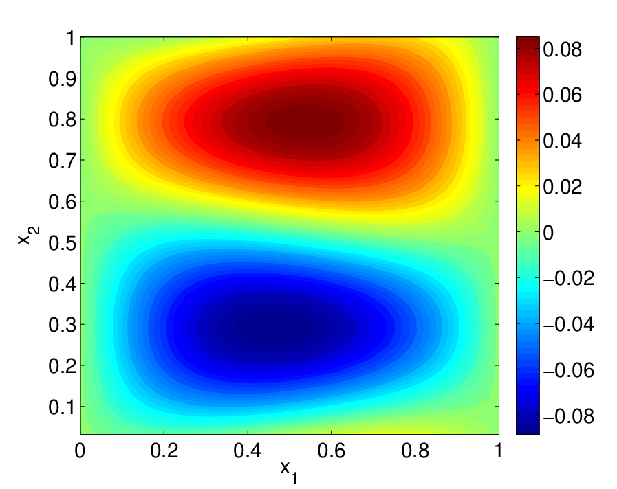
while $\Delta T=T^{+}-T^{-}$ varied across the instability region. Note that this lies in the region $L_{2}<2\sqrt{2}L_{1}$, thus the primary instabilities come from the lowest spatial harmonics as proven in Theorem 4. All the simulations were made with $N_{x_{1}}=N_{x_{2}}=32$, though we selectively checked with $N_{x_{1}}=N_{x_{2}}=64$.

In Figure 2 we plot two periodic travelling wave solutions near the upper stability threshold $\Delta T_{2}\approx 0.162$ and further inside the nonlinear regime as can be seen by the locus of parameters in Figure 3(a). The weakly nonlinear solution for $\Delta T\approx\Delta T_{2}$ closely resembles the unstable eigenfunction, while the solution further inside the nonlinear regime has a clear nonlinear structure.

In order to trace the stable branches of solutions bifurcating from the supercritical Andronov-Hopf bifurcations at $\Delta T=\Delta T_{1},\Delta T_{2}$, we perform a simple continuation: for $\Delta T$ near the bifurcation at $\Delta T_{1}$, we simulate an initial condition close to $\rho_{ss}$ and after a long transient compute the sup-norm over a long time interval. We then slightly increase $\Delta T$ and repeat this step with the initial condition being the solution at the final time of the previous step. In this way we obtain the bifurcation diagram in Figure 3, where the numerical instability thresholds are in very good agreement with the analytical ones.

As predicted by Theorem 7, the slope of the resulting curve is larger near the left endpoint of the instability region than near the right endpoint. Further away from these endpoints, the solution shapes change and we conjecture a period doubling bifurcation near $\Delta T=0.0646$, rapidly followed by a torus bifurcation. This would be consistent with the sharper increase in the sup-norms in Figure 3, and the fact that the periods of the solutions become rather large, see Figure 4(b). Despite this detour to another attractor, the solution is eventually turning into the near harmonic periodic solution bifurcating from the right endpoint $\Delta T_{2}$, see Figure 2 (a).

As an example for instabilities caused by higher spatial harmonics, we plot in Figure 5 a solution that emerged from an instability with wavenumber $k_{2}=2$.

For the bifurcation study it is convenient to formulate (1) through the deviation $u=(u_{1},u_{2})$ from $\rho_{ss}$,

In terms of $u$, and in the comoving variable $x_{2}\to x_{2}+T^{-}t$, system (1) reads

subject to (periodic b.c. in $x_{2}$ and) homogeneous Dirichlet boundary conditions

Next we choose a simple functional analytic setting for a formulation of (6) as a parabolic problem by solving the Poisson equation. This is convenient for the center manifold reduction, but also gives a simple well-posedness setting.

Let $\Omega:=[0,L_{1}]\times[0,L_{2}]$ and denote the Sobolev spaces ${\sf H}^{j}=H^{j}([0,L_{1}]\times\mathbb{R}/L_{2}\mathbb{Z})$ as well as

which incorporate the Dirichlet boundary conditions. We shall use standard notation: for $f_{1}$, $f_{2}$ $\in{\sf L}^{2}([0,L_{1}]\times\mathbb{R}/L_{2}Z)$ we denote the scalar product by $\langle f_{1},f_{2}\rangle=\int_{\Omega}f_{1}(x)\overline{f_{2}(x)}dx$ and for $\mathrm{f}_{j}=(\mathrm{f}_{j,1},\mathrm{f}_{j,2})\in L^{2}([0,L_{1}]\times\mathbb{R}/L_{2}Z)^{2}$ $j=1,2$ by $\langle\mathrm{f}_{1},\mathrm{f}_{2}\rangle_{2}=\langle\mathrm{f}_{1,1},\mathrm{f}_{2,1}\rangle+\langle\mathrm{f}_{1,2},\mathrm{f}_{2,2}\rangle$.

Thanks to these boundary conditions, we can solve the Poisson equation in (6); see also §4 for explicit solutions. We thus obtain $E$ via the bounded operators $A_{j}:Z\to{\sf H}^{3}$ defined by

Notably, $A_{2}$ in fact maps into $Z$, because $E_{2}=\partial_{x_{2}}V$ vanishes for $x_{1}=0,L_{1}$ due to the Dirichlet boundary conditions.

In order to apply standard results on parabolic equations, let us write (6) equivalently in the standard form

so that solutions of this and (1) are in 1-to-1 correspondence. Here

Note that ${\bf L}\in\mathcal{L}(Z\times Z,X\times X)$ is the linearization of (1) in $\rho_{ss}$. We have that $R:Z\times Z\to Y\times Y$ since $\nabla u_{j}$ vanish at $x_{1}=0,L_{1}$ and ${\sf H}^{2}$ is a Banach algebra; $R$ is in fact analytic in $u$. See also §5. Moreover, the imbeddings $Z^{2}\hookrightarrow Y^{2}\hookrightarrow X^{2}$ are dense and the uniformly elliptic operator $-{\bf L}:Z\times Z\subset X\times X\to X\times X$ is a sectorial operator, generating an analytic semigroup, and so (6) admits mild and classical solutions $u(t)$ for any initial condition $u(0)\in Y\times Y$. The sectoriality is a consequence of the fact that the laplacian is sectorial in $Y$ with domain ${\sf L}^{2}$ of the cylinder [5], and this is robust under addition of the lower order terms in ${\bf L}$. It thus also possesses a square root, which then provides an isomorphism from ${\sf L}^{2}$ to $X$. Hence, ${\bf L}$ is also sectorial on $Z$ with domain $X$. Note also that ${\bf L}$ has a compact resolvent and thus discrete spectrum accumulating at $-\infty$. We discuss its spectrum in detail in the next section.

For the bifurcation analysis, we distinguish the stable spectrum of ${\bf L}$, $\sigma_{-}({\bf L}):=\{\lambda\in\sigma({\bf L}):\Re\lambda<0\}$, its neutral spectrum $\sigma_{0}({\bf L})=\{\lambda\in\sigma({\bf L}):\Re\lambda=0\}$ and its unstable spectrum $\sigma_{+}({\bf L})=\{\lambda\in\sigma({\bf L}):\Re\lambda>0\}$.

The next Lemma characterizes the spectrum and is the basis for the identification of bifurcations. While this concerns the comoving variable of system (6), the spectrum for the original system is the same up to a scaling of the imaginary parts. See §6.

We will start to discuss the relevance and implications of this result after the proof. In preparation of the proof, choose the orthogonal basis of $X$ given by

where $k\in\mathbb{N}_{*}\times\mathbb{Z}$. In order to express the operator $A$, denote

Indeed, if $f\in X$, the explicit solution to the Poisson equation $-\nabla^{2}V=f$ in terms of this basis reads

We therefore get the explicit formula for $A$:

Note that the proof also implies that eigenfunctions of ${\bf L}$ have the form

with $\xi_{k}$ a eigenvector of $M_{k}$.

The last statement in Lemma 1 means that only $D_{k}>0$ and $\lambda_{(1,k_{2})}^{+}$ with $k_{2}\in\mathbb{Z}\setminus\{0\}$ allow for destabilization, and the real part in this case is given by

Note that this is a function of the three parameters $\nu/L_{1}^{2}$, $\Delta T/L_{1}$, $(k_{2}/\ell)^{2}$. As expected, increasing viscosity always stabilizes, with increasing impact for increasing $(k_{2}/\ell)^{2}$. However, the dependence of the real part on $k_{2}/\ell$ is not necessarily monotone, which allows for intricate destabilization scenarios.

The imaginary part, $\Im(\lambda_{(1,k_{2})}^{+})$, is never zero, which means that all bifurcations are non-stationary and we generically expect Andronov-Hopf bifurcations, where $k_{2}$ determines the wavenumber of bifurcating solutions.

We consider the temperature difference $\Delta T$ as the primary bifurcation parameter and therefore focus on the location of instabilities as $\Delta T$ varies, as well as on the wavenumber of destabilizing modes determined by $k_{2}$.

In Figure 6 we plot sample computations of spectrum as $\Delta T$ varies, illustrating the stabilizing effect of the viscosity. Crossings of eigenvalue curves at zero real part can occur, which is expected to generate rich bifurcations. However, in this paper we focus on simple Andronov-Hopf bifurcations.

Recall the spectral conditions at a primary Andronov-Hopf bifurcation

and in the nondegenerate case, the critical eigenvalues transversely cross the imaginary axis upon parameter variation.

It turns out that we can characterize a large part of parameter space, where critical eigenvalues have $k_{2}=1$, that is, $k=k_{c}:=(1,1)$. We therefore define the following particular case of (21).

Here and in the following we denote $\overline{\kappa}=(\kappa_{1},-\kappa_{2})$ for $\kappa\in\mathbb{R}^{2}$.

Rearranging sign conditions on (20) and squaring, we readily compute that the sign of $\Re(\lambda_{(1,k_{2})}^{+})$, for $\kappa_{2}=k_{2}^{2}$ is the sign of

which is somewhat simpler to handle. In particular, zeros of $d$ are the critical eigenvalues for bifurcations. This yields the following a priori bounds on $\Delta T$ for linear instability.

Note that $d(\cdot,\kappa_{2})$, as a quadratic polynomial in $\Delta T$, has two real roots $\Delta T_{1}(\kappa_{2})\leq\Delta T_{2}(\kappa_{2})$ if and only if the viscosity is sufficiently small,

with a double root at equality. Hence, this is a necessary and sufficient condition for the occurrence of critical eigenvalues $\lambda_{(1,\sqrt{\kappa_{2}})}^{+}$ as $\Delta T$ varies. However, it is subtle to determine when the critical eigenvalues destabilize the equilibrium as this requires to exclude unstable eigenvalues for all other $k_{2}$.

Nevertheless, the location of these parabola’s maxima in $\Delta T$ is at

which is strictly decreasing in $\kappa_{2}$. Therefore, the $k_{2}$-value of these parabola in $\Delta T$ can be identified by the relative location of their maxima.

The geometric nature of bifurcating solutions is determined by the $k_{2}$-value of critical and destabilizing eigenvalues as $\Delta T$ in- or decreases from outside $[0,4L_{1}/\pi^{2}]$. We thus define

To ease notation, we simply write $\Delta T_{j}$ for $\Delta T_{j}(1)$, $j=1,2$.

As a first step to understand the nature of destabilizing $k_{2}$-instability regions, we consider the case $k_{2}=1$ and in preparation define the following condition.

Note that Hypothesis 2 requires a ratio of temperature difference and viscosity to dominate a ratio involving domain geometry and linear mode harmonics.

The point of the theorem is that it provides conditions (Hypothesis 2 or $\ell\leq 2\sqrt{2}$) under which the destabilizing mode for increasing and decreasing $\Delta T$ is known, namely the lowest spatial harmonic. Note that the values of $\ell$ in particular include the case $\ell=1$ considered in [3].

Now, we are going to present a condition, which guarantees that other destabilization scenarios also occur.

This means that the $1$-instability region is not primary. In fact, it is also not primary for nearby parameter values that produce $\Delta T_{2}(4)>\Delta T_{2}(1)$. The solution to (27) for $\kappa_{2}=4$ is $\ell_{4}\approx 5.37$, and for $\kappa_{2}=9$ it is $\ell_{9}\approx 7.22$. See Figure 7. For $\ell$ between these value (and slightly above $\ell_{9}$), we numerically find that the $2$-instability region is primary. We omit the tedious analysis. In general, for any given $k_{2}$ Hypothesis 2 is violated for sufficiently large $\ell$ (with $\nu,L_{1}$ fixed), since $\Delta T$ is bounded (Lemma 2).

For the case of small viscosity (and $\ell>2.8$), we omit the somewhat tedious detailed analysis for the destabilizing left endpoint. However, we immediately obtain the following.

Lastly, we point out the possibility of multiple disjoint primary $k_{2}$-instability regions, where changing $\Delta T$ destabilizes and stabilizes multiple times. In Figure 8 we plot eigenvalue curves, where two $k_{2}$-instability regions consist of a point. Parameters $\nu=\nu_{\mathrm{crit}}(k_{2})=\nu_{\mathrm{crit}}(k_{2}^{\prime})$ and $\ell$ that produce such scenarios can be readily computed from (23); here we take $k_{2}=1$, $k_{2}^{\prime}=4$. For perturbed $\nu<\nu_{\mathrm{crit}}(1)$ the instability regions become disjoint open intervals.

In this section, we consider the vicinity of parameters with critical $\Delta T=\Delta T_{j}$ for $j=1$ or $j=2$ and assume that no other eigenvalues lies on the imaginary axis. The main example is a primary $1$-instability region. For the unfolding of the bifurcation in the generic case $\Delta T_{1}<\Delta T_{2}$ we introduce the parameter $\mu_{1}$ by $\Delta T=\Delta T_{j}+\mu_{1}$. In the degenerate case $\Delta T_{1}=\Delta T_{2}$, where $\nu=\nu_{\mathrm{crit}}(1)$, we additionally unfold with $\mu_{2}$ defined by $\nu=\nu_{\mathrm{crit}}(1)-\mu_{2}^{2}$. For readability we frequently suppress the index $j$.

References

- [1] Robert A. Adams and John J. F. Fournier, Sobolev spaces, second ed., Pure and Applied Mathematics (Amsterdam), vol. 140, Elsevier/Academic Press, Amsterdam, 2003.
- [2] Emmanuel Grenier, On the nonlinear instability of Euler and Prandtl equations, Comm. Pure Appl. Math. 53 (2000), no. 9, 1067–1091.
- [3] Daniel Han-Kwan, On the confinement of a tokamak plasma, SIAM J. Math. Anal. 42 (2010), no. 6, 2337–2367.
- [4] Mariana Haragus and Gérard Iooss, Local bifurcations, center manifolds, and normal forms in infinite-dimensional dynamical systems, Universitext, Springer-Verlag London Ltd., London, 2011.
- [5] Daniel Henry, Geometric theory of semilinear parabolic equations, Lecture Notes in Mathematics, vol. 840, Springer-Verlag, Berlin, 1981.
- [6] M. A. Malkov and P. H. Diamond, Weak hysteresis in a simplified model of the L-H transition, Phys. Plasmas 16, 012504, 2009.
- [7] F. Wagner, A quarter-century of H-mode studies, Plasma Phys. Control. Fusion 49 B1, 2007.