Reachability via Compositionality in Petri nets
Abstract
We introduce a novel technique for checking reachability in Petri nets that relies on a recently introduced compositional algebra of nets. We prove that the technique is correct, and discuss our implementation. We report promising experimental results on some well-known examples.
Introduction
We introduce a novel technique for checking reachability in 1-bounded Petri nets. Our approach relies on a structural decomposition of nets, using the algebra of nets with boundaries developed in [18, 1, 2] and the algebra of labelled transition systems (LTS) originally developed in [10]. After explaining the intuitions and some motivating examples, we prove the technique correct, discuss our implementation and report on experimental results.
Many asynchronous systems are regular in their structure, in the sense that they can be considered as a suitable composition of several identical, communicating components. In many such systems, the communication between individual components can be characterised using relatively small (w.r.t. the size of the global state space) amounts of information, and as a consequence, the reachability of a particular global state can be checked locally. The algebra of nets with boundaries allows us to capture precisely how separate “component nets” communicate with each other.
To illustrate the ideas that underlie our approach we introduce the simple, well-known11 1 For example, see [7, Fig. 6]. bounded buffer net, , illustrated in the left part of Fig. 1. We wish to check whether the “opposite” marking is reachable—that is, the places in the lower row are to be marked and the places in the upper row are to be unmarked. Taking a global view, a simple calculation confirms that the length of the firing sequence necessary to reach the desired marking is quadratic in (see Fig. 8(a)). We will, instead, check for reachability locally, component-wise, so imagine that the net is “split” into two nets and , sharing the transition , as in the right part of Fig. 1.
Remark 1
Observe (1) that and can proceed independently to reach the desired local marking, only “synchronising” on and (2) the “synchronisation policy” is quite simple to describe. Indeed, can fire its local copy of an arbitrary number (including 0) of times during a successful computation; can reach its desired marking after firing its copy of at least twice, after which can be fired an arbitrary additional number of times. These two “policies” are clearly compatible, meaning that the entire net can reach its global desired marking.
To make the above intuitions precise, we recall the algebra of nets introduced in [18]. We will use a non-standard graphical representation of nets, more suited for illustrating the operations of the algebra: is rendered with the alternative graphical notation in the left-most diagram of Fig. 2. Transitions are represented using undirected links and each link can be connected to an arbitrary number of ports. Each place has two ports: one for incoming transitions, illustrated with a triangle pointing into the place, and one for outgoing transitions, illustrated with a triangle pointing out of the place. Thus the pre-set of a transition is the set of places to which it is connected via their outgoing port, and its post-set is the set of places to which it is connected via their incoming port. Transitions can also be connected to boundary ports, which serve as an interface between nets with boundaries. The net can be expressed as the composition ; the individual components , and are illustrated in Fig. 2. The operation ‘’ that composes two nets along a compatible, common boundary is defined formally in §1.1.
Each component net with boundaries, together with its initial marking and desired local marking, can be translated to a non-deterministic finite automaton (NFA), with states being the reachable markings, and transitions the boundary interactions observed when net transitions fire. The initial state is the initial marking and the final state is the desired marking. We illustrate22 2 All illustrations of automata were generated with GraphViz (http://www.graphviz.org). For space-efficiency, transitions are annotated with sets: , representing the existence of two transitions, labelled respectively and . We use in the labels as shorthand for any choice of and . this translation in Fig. 3. For example, in the translation of , state corresponds to the initial marking and state to the desired complementary marking. The labels of transitions are, in general, pairs of binary strings and , written , representing interaction on the left () and the right () boundaries. The concept of “interaction on a boundary” is important and we will explain it further below. To guarantee compositionality, we must use an underlying step firing semantics of nets, i.e. a transition in the NFA witnesses the firing of a (possibly empty) set of independent transitions within the component net. Returning to the translation of : the labelled NFA-transitions in state and witness the possibility of no behaviour (i.e. the empty set of net-transitions firing) with the label signifying that no net-transitions connected to either boundary were fired. The NFA-transition witnesses that the right hand side net-transition has fired and produced the desired marking. The fact that the fired transition is connected to the port on the right boundary is recorded by in the transition label. The remaining NFA-transition is symmetric.
 |
The principle of compositionality, proved in Theorem 1.1, is illustrated in Fig. 4: given two nets, we can obtain the NFA representing their (composite) behaviour in two ways: 1) compose two nets to form the net , and then generate its NFA, or equivalently, 2) generate the two (identical) NFAs for each and compose them, using a variant33 3 iff . of the product construction. Compositionality ensures that the diagram commutes, in other words, the global behaviour of the composition of the two nets is completely determined by the behaviour of the individual nets, when synchronised along their common boundary.
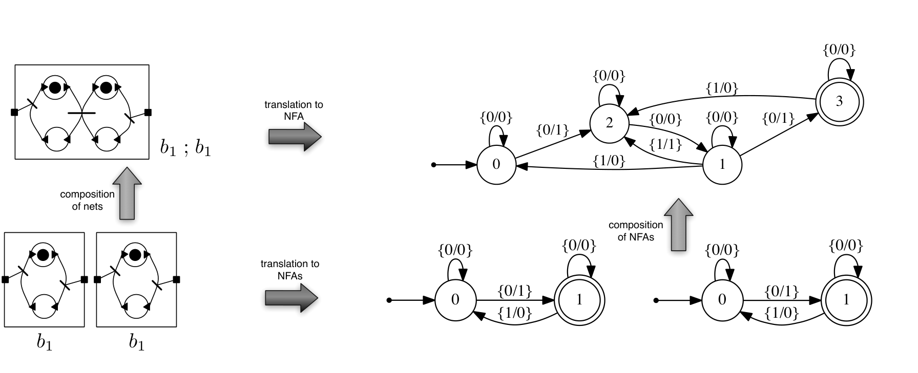 |
The NFA generated for ( composed times) has states, thus directly computing the automaton for is feasible only for small . Fortunately, to generate a correct NFA of the composite net, it is sufficient to capture how each component net must interact on its boundaries in order to reach its local desired marking—its “synchronisation policy”. To do this, we close the NFA with respect to internal (-) moves—those transitions labelled solely with s, signifying no interaction at the boundaries—to obtain an automaton with the same states, but with transitions being paths . We then minimise the new NFA, obtaining a deterministic automaton (DFA), with an “error” state that is reached whenever an illegal (i.e. not in the behaviour of the underlying net) interaction is observed on the boundaries. This DFA minimally represents the entire behaviour (assuming that an observer may only observe traces) of the net, w.r.t. interactions on its boundaries.
Note that the states of the NFA obtained from a net are 1-1 with the reachable markings of the underlying net; in general, this is not the case after -closure and minimisation: the states of the minimal DFA merely capture the “protocol” the net must follow when interacting with its environment, in order to arrive at the desired marking. Indeed, for , the resulting minimal DFA has states. Of course, computing the minimisation of an NFA can be very expensive—in the worse case, triple exponential in the number of places of the original net—our strategy is thus roughly to decompose nets as far as possible (thereby only minimising small NFAs) and take advantage of any regular, repetitive structure in the net, via memoisation. As discussed, compositionality guarantees correctness—the fact that the square in Fig. 5, illustrating the process for , commutes is a consequence of Theorems 1.2 and 1.3.
 |
The applicability of our approach depends on finding “good” decompositions of nets. For , there are many potential decompositions: the optimal44 4 All experiments were run on an Intel i7-2600 3.40GHz CPU, 16GB of RAM, running 64-bit Ubuntu Linux. is the 1st decomposition in Fig. 6, which corresponds to the algebra term . Indeed, the composition of and minimises to the trivial accepting automaton; Fig. 7 contains illustrative translation steps of the different decompositions of . In (i) the composition of the automaton for is composed with the automaton for : after minimisation we again obtain the automaton for . Thus the procedure reaches a fixed point after the first step, as illustrated in (ii). This fact formally captures the intuition about given in Remark 1. For this decomposition, memoisation guarantees that the composition and minimisation is performed only once. In particular, this means that checking reachability for , given this decomposition, is linear in . However, other decompositions do not lead to such good performance. In particular, consider the 2nd decomposition of Fig. 6; here, memoisation does not help (we obtain a different NFA composition after each step) and we must perform minimisation after each composition, as illustrated in steps (iii) and (iv) of Fig. 6.
Our automated approach to deconstructing (discussed in §2.1) produces the 3rd (balanced) decomposition of Fig. 6. In this particular case we decompose by identifying a transition that connects two components of similar size. This decomposition, while not optimal, allows frequent use of memoisation, reducing the amount of computation. A table of running times for the construction of a minimal DFA for , following the three decompositions of Fig. 6, is given in Fig. 8(a).
 |
| min # | Time [s] | |||
|---|---|---|---|---|
| n | firing sequence | right | left | balanced |
| 16 | 136 | 0.000 | 0.020 | 0.008 |
| 32 | 528 | 0.000 | 0.140 | 0.024 |
| 64 | 2080 | 0.000 | 1.108 | 0.172 |
| 128 | 8256 | 0.000 | 12.597 | 2.954 |
| 256 | 32896 | 0.000 | - | 74.737 |
| 65536 | 2147516416 | 0.228 | - | - |
| n | # places in net | min # firing sequence | time [s] |
|---|---|---|---|
| 6 | 63 | 120 | 0.028 |
| 8 | 255 | 502 | 0.088 |
| 10 | 1023 | 2036 | 0.312 |
| 12 | 4095 | 8178 | 1.332 |
| 14 | 16383 | 32752 | 5.864 |
| 16 | 65535 | 131054 | 25.014 |
We have illustrated how the operation ‘’ allows decomposition of the net in order to exhibit its the regular structure. We will briefly consider a second example that illustrates the use of the second operation of the algebra, ‘’. Consider the net in Fig. 9, where we want to check whether all the places can be marked; N.B this net is not 1-safe, but 1-boundedness means that a transition is blocked if there is a token present in its post-set. Our automated procedure constructs the decomposition illustrated in the right part of Fig. 9. In Fig. 13 we illustrate the steps involved in calculating the minimal DFA for , and give a table of experimental results in Fig. 8(b).
Structure of the paper.
In §1 we study the foundations of our technique and prove it correct. In §2 we discuss our implementation and give additional experimental results. Connections with related work are in §3, and we conclude with directions for future research in §4. Due to space constraints, proofs and non-essential figures have been moved to the appendix.
1 Nets with boundaries
In this section we give the theoretical underpinnings of our technique, harnessing the compositionality of the algebra of nets with boundaries in order to prove its correctness.
Notational conventions.
For let . We write for the powerset of . We write for the set . Given and we write . We identify binary strings of length with subsets of in the obvious way: iff .
Definition 1
A net with boundaries is where:
- -
is the set of places, is the set of transitions
- -
are, respectively, the left and the right boundaries
- -
give, respectively, the pre- and post-sets of each transition
- -
and connect each transition to, resp., the left and the right boundary.
Additionally, we assume55 5 That is, at most one transition can be connected to any place on the boundary. This assumption allows us to simplify the definition of composition of nets; for the more general case see [2]. that for any , and . Ordinary Petri nets can be considered as nets with no boundaries.
We must use step semantics of nets instead of the more common interleaving semantics to guarantee compositionality; we will illustrate this in Remark 2. Let . Transitions are said to be independent when . A set is said to be mutually independent (MI) when for all , and are independent. For sets of transitions we will abuse notation and write , and similarly for , and .
Each net with boundaries determines an LTS whose transitions witness the step semantics of the underlying net, originally described by Katis et al [9]. For the 1-bounded case, the labels are pairs of binary strings of length and , respectively. The states are markings of , denoted by , where . The transition relation is defined:
1.1 Composition of nets with boundaries
Suppose that and are nets with boundaries. A synchronisation is a pair where and are MI sets of transitions, with . Given synchronisations and , we say exactly when and . The trivial synchronisation is . A synchronisation is said to by minimal when it is non trivial and, for all synchronisations , if then is trivial. The set of minimal synchronisations of and is denoted . The composed net has:
- -
as its set of places,
- -
as its set of transitions. Given we let , , and .
Examples of compositions of the net are given in Figs. 2 and 6. Another example is given in Fig. 10, with the resulting transition arising from the minimal synchronisation .
Remark 2
The example in Fig. 10 illustrates the necessity for step semantics in order for compositionality to hold. Indeed, in the composition we have the transition that witnesses the firing of its transition. This transition decomposes into and . The first of these requires the simultaneous firing of and in ; thus if we had considered interleaving semantics then compositionality would fail in this example.
The next result is a special case of [2, Theorem 3.6], where a more general algebra of nets is considered. We will rely on this to prove the correctness of our technique in Theorems 1.2 and 1.3.
Theorem 1.1 (Compositionality)
Suppose that and are nets with boundaries. The following holds for all , , and :
∎
The conclusion of Theorem 1.1 implies that, for instance, bisimilarity is a congruence w.r.t. to ‘’. For the purposes of reachability checking, traces are sufficient.
Corollary 1
There exists a trace iff there exist traces and . ∎
In particular, to check for reachability in a composed net, it suffices to find computations in the components that agree on their shared boundary.
The other operation on nets with boundaries is , which can be understood as a parallel composition of nets. Given and , has:
- •
as its set of places,
- •
as its set of transitions. , , and similarly for and . Instead while ; similarly and .
Compositionality also holds w.r.t. : iff and . Due to space constraints we omit the details here; they are straightforward as there is no interaction between the two nets.
1.2 From nets with boundaries to NFAs
By an NFA with boundaries we mean an NFA with set of labels , written , where and . Given NFA with boundaries and , the NFA with boundaries is obtained by a variant of the product construction where iff there exists such that and . Given NFA with boundaries and , the NFA with boundaries is obtained via another variant of the product construction: here iff and . The algebra of automata with boundaries described above is an instance of Span(Graph) [10].
Given a net with boundaries , and non-empty sets of, respectively, initial and final markings, we can consider its labelled transition system as an NFA, written , that has initial states and final states . If does not have any places then has exactly one state, which is an accept state (see NFA for , in Fig. 3). The following is immediate.
Proposition 1
Given , initial and final markings , a marking in is reachable from a marking in iff . ∎
We also have the following as an immediate consequence of Theorem 1.1:
and in particular the two automata accept the same language.
1.3 Weak closure and minimisation
Hiding internal computations in individual component nets is crucial for the performance of our technique. The procedure is akin to the -reflexive-transitive closure of an LTS , which yields an LTS on which bisimilarity agrees with weak-bisimilarity on , in the sense of Milner [13].
Let . Sometimes we will write simply when and are clear from the context. Notice that given any net , for each marking there is a transition that arises from firing the empty set of net-transitions. In general, transitions witness the firing of “internal” net-transitions in , ie those that are not connected to any boundary port.
The weak transition system induced by has transitions:
| (1) |
Note that the above notion of weak transition differs from that considered in [2] but is close to the weak transitions of [17].
Theorem 1.2 (Compositionality w.r.t. weak semantics)
Suppose that and are nets with boundaries. Then for all , , , :
- (i)
if then , for and
- (ii)
if and for some then . ∎
Given an NFA with boundaries , let denote the DFA obtained by -closure and minimisation.
Remark 3
Recall that any ordinary net can be considered as a net with boundaries . Now is one of two DFAs: the DFA with one accept state (if a marking in is reachable from some marking in ) and the DFA with one non-accept state (if no markings in are reachable from any marking in ).
Given an ordinary Petri net , initial markings and final markings , a simple but extremely inefficient way of checking the reachability of a marking is thus to directly compute and check whether the single state in the resulting DFA is an accept state. Our technique for checking reachability is based on computing this DFA using a structural decomposition of , which, when combined with memoisation, can result in fast execution times.
1.4 Correctness
Here we give a formal account of our technique and prove it correct, using the previous results in this section. A wiring expression is a syntactic term formed from the following grammar
where the leaves are variables. A variable assignment is a map that takes variables to nets with boundaries. Given a pair of a wiring expression and variable assignment , its semantics is a net with boundaries, defined recursively in the obvious way: , and . We implicitly assume that variable assignments are compatible with , in the sense that only nets with a common boundary are composed; we leave out the formal details, which are straightforward. Given a net , we say that is a wiring decomposition of if .
Given a wiring decomposition of , together with maps , called, respectively, initial markings and final markings, that take each variable to a set of markings of the net , define recursively:
The function is the formalisation of our approach, taking a wiring decomposition, together with initial and final markings to a minimal DFA. Sets of markings of the leaf nets given by and can be combined to form a set of markings of in an obvious way: , , (and similarly for .)
Theorem 1.3 (Correctness)
Suppose is a wiring decomposition of , initial markings and final markings. Then .∎
2 Implementation and experimental results
Our implementation has been written in Haskell, and is available for download66 6 http://users.ecs.soton.ac.uk/os1v07/ICALP13. The high level view of our algorithm is:
- 1.
As input, take an ordinary marked net (considered as a net with boundaries ) and a target marking, given place-wise, to be checked for reachability. Concretely, each place is labelled with ‘Yes,’ (token must be present) ‘No’ (token must be absent) or ‘Don’t care.’
- 2.
- 3.
Taking advantage of memoisation—to eliminate duplicate computations—traverse the wiring decomposition tree to compute :
- (a)
- (b)
At a composition node, we generate the NFAs corresponding to each sub-tree, and compose them using the variant of product-construction discussed in §Introduction, finally closing and minimising the resulting NFA.
- (c)
At a tensor node, we generate the NFAs corresponding to each sub-tree, combine them using the standard product construction on NFAs, and perform minimisation.
The experimental results given in Figs. 8 and 12(b) are given for pre-constructed decompositions, that is, only step 3 of the algorithm is performed. The results in Fig. 12(a) were obtained using the implementation of the full algorithm.
2.1 Decomposer
Our net decomposition algorithm attempts to find decompositions via two simple approaches: first we look for a net-transition that, when removed, results in two disconnected nets. If many such transitions exist then we take the one that results in the most balanced (in number of places) decomposition. An example is the balanced decomposition in Fig. 6. If such a transition cannot be found, we look for a place that, once removed, results in two disconnected nets. This results in a ‘’ node (that results from removing the place) followed by a ‘’ node (that composes the two disconnected nets). Again, if many such places exist, we look for one that results in the most balanced decomposition. An example of this decomposition strategy is the decomposition in Fig. 9. Both searches are quadratic in the size of the net. If neither a suitable transition nor place is found, we remove a place that results in the smallest boundary, after decomposition. The time taken to decompose the net is given in Fig. 12(a); in this example the time to decompose the net dominates. Note that, given a net, a decomposition must be computed (or given as input) only once, whence different various initial markings and desired markings can be considered.
2.2 NFA closure and minimisation
Our approach relies on ignoring internal computations to reduce the state space to be explored. To produce minimal DFAs for an input NFA, we apply epsilon closure, and minimisation, as detailed in §1.3. We perform epsilon closure through a variant of the subset-construction on NFAs, which constructs the NFA of sets of states reachable through or standard transitions, starting from the closure of the initial states of the input NFA. To perform minimisation we employ the well-known algorithm of Brzozowski [3].
A notable implementation detail is that we use a variant of Reduced Ordered Binary Decision Diagrams (ROBDD, commonly written as BDD) to encode the transition relation of the NFA—the labels of our transitions are binary strings and thus any state gives rise to a function . Traditionally, BDDs are used to provide compact representations for functions , but we found it a straightforward exercise to generalise from the boolean algebra of the booleans to the boolean algebra of subsets.
2.3 Experimental results and discussion
In addition to the results in Fig. 8 we considered a standard net encoding of the dining philosopher problem. Given the nets in Fig. 11, let , . Then a table of dining philosophers can be obtained as:
| (2) |
Running times, when checking for deadlock in , are given in Fig. 12(b). The slow growth w.r.t. illustrates the fact that our technique works well when a fixed point is quickly reached when traversing a wiring decomposition, for example, the right decomposition of in Fig. 6 reaches a fixed point after one ‘’ node in the wiring decomposition. The fixed point for (2) is reached when calculating : the resulting minimal DFA has 10 states, as shown in Fig. 15. Intuitively, this means that while one can distinguish between 1, 2 and 3 philosophers via interaction on the boundary, all reduce to the same minimal DFA for . Our procedure takes advantage of this: memoisation of compositions means that we minimise only once.
| n | deconstruction [s] | NFA generation [s] |
|---|---|---|
| 4 | 0.052 | 0.008 |
| 5 | 0.240 | 0.008 |
| 6 | 1.108 | 0.004 |
| 7 | 5.104 | 0.008 |
| 8 | 23.261 | 0.008 |
| 9 | 103.106 | 0.012 |
| 10 | 451.628 | 0.012 |
| n | time [s] |
|---|---|
| 1 | 2.072 |
| 4 | 3.844 |
| 16 | 3.924 |
| 64 | 3.920 |
| 128 | 3.908 |
| 256 | 3.908 |
| 1024 | 3.684 |
Many nets are not amenable to efficient decomposition and are unsuitable for our technique. For instance, our implementation performs poorly when input nets are cliques, nets where every place is connected to every other by a transition, or in general, on “densely connected” nets. One reason why our technique is infeasible for such nets is because two factors influence the size of the generated NFA from a net : (i) the number of places—if has places, this can translate to potentially NFA-states, and (ii) the size of the net boundaries, since it implies an alphabet of size up to . In fact, even with hand constructed decompositions, our implementation fails to terminate even for very small cliques due to large boundaries in any decomposition.
3 Related work
Algebras of nets and automata.
The algebra of automata with boundaries used in this paper is an instance of the algebra of Span(Graph) [10], developed by R.F.C. Walters and collaborators: in fact, a translation from nets to this algebra was already present in [9]. The goal of the more recent work [18, 1, 2] was to lift this algebra to the level of nets in a compositional way, study the resulting behavioural equivalences and explore connections with process algebra. A theme of our work is to ignore state and focus on external interactions: here we were inspired by the ideas of Milner [13]. Conceptually related approaches in semantics of programming languages include [15, 8].
Reachability
in bounded, finite state Petri nets is a widely-studied problem and there are several well-known approaches to mitigating the impact of state-explosion (it follows from [4] that the problem is PSPACE-complete.) Due to space constraints we are able to offer only cursory overviews and comparisons of techniques that are most related to our approach. A well-known technique is partial order reduction: in a seminal paper, McMillan [12] used the unfolding construction [14] in order to analyse reachability in Petri nets by generating finite complete prefixes, that is, initial parts of unfoldings that suffice for reachability. The algorithm to compute the finite complete prefix was later improved [7, 11]. Unfoldings (and finite complete prefixes) carry more information about the computations of nets than merely reachability, for instance, allowing LTL model checking [5]. For an overview of the extensive field see [6]. A finite complete prefix must be constructed prior to a reachability analysis, analogously to our construction of a wiring decomposition prior to translation. Because of the different nature of the two approaches, it is difficult to offer a thorough analysis of the relative performance of the two approaches: on some of the examples we have considered the performance of our implementation is competitive (compare Fig. 8(a) with [7, Table 1].) Another technique, known as symmetry reduction [19, 16], exploits symmetries in the state space: the goal is, roughly, to build a reduced reachability graph in order to visit only one representative from each orbit. Our use of memoisation is similar in spirit to symmetry reduction, since we only need to translate any particular wiring decomposition once.
In experiments (, , and others) our implementation often performs well in identifying unreachable configurations; this is because in many systems the reasons for a configuration being unreachable are “local”. Here our approach contrasts with techniques such as unfolding or symmetry reduction where (efficient representations of) explicit reachability graphs are constructed.
4 Conclusions and future work
We have introduced a new technique for reachability in bounded Petri nets, based on (i) structural decomposition using a recently developed compositional algebra and (ii) avoiding state explosion by focusing only on interactions between component nets, forgetting internal state. Our technique depends on finding efficient decompositions and works best when the computation reaches fixpoints w.r.t. interactions on boundaries in composed systems, as illustrated in the examples that we have highlighted. We have proved that the technique is correct, implemented it and performed a number of experiments. Finally, we have developed and implemented an algorithm for automatic decomposition of nets that performs adequately on a number of examples.
In future work we plan to improve our decomposition algorithm and characterise the class of nets to which our approach is suited. Additionally, by using the full algebra [18, 2] of nets, in particular, the possibility of connecting several transitions to the same boundary port, we hope to alleviate some of the problems identified in §2. We also plan to generalise our approach to other models: for example by examining symbolic representations of the algebras of P/T nets in [1, 2] we hope to extend our technique to coverability.
References
- [1] R. Bruni, H. C. Melgratti, and U. Montanari. A connector algebra for P/T nets interactions. In Concurrency Theory (CONCUR ‘11), volume 6901 of LNCS, pages 312–326. Springer, 2011.
- [2] R. Bruni, H. C. Melgratti, U. Montanari, and P. Sobociński. Connector algebras for C/E and P/T nets’ interactions. LMCS, 2012. 56 pages, submitted.
- [3] J. Brzozowski. Canonical regular expressions and minimal state graphs for definite events. In Mathematical Theory of Automata, volume 12 of MRI Symposia, pages 529–561. Polytechnic Press, 1962.
- [4] A. Cheng, J. Esparza, and J. Palsberg. Complexity results for 1-safe nets. In FSTTCS, volume 761 of LNCS, pages 326–337, 1993.
- [5] J. Esparza and K. Heljanko. Implementing LTL model checking with net unfoldings. In SPIN, volume 2057 of LNCS, pages 37–56, 2001.
- [6] J. Esparza and K. Heljanko. Unfoldings: a partial-order approach to model checking. Springer, 2008.
- [7] J. Esparza, S. Römer, and W. Vogler. An improvement of McMillan’s unfolding algorithm. Form Method Syst Des, 30(3):285–210, 2002.
- [8] D. R. Ghica and G. McCusker. The regular-language semantics of second-order idealised ALGOL. Theor. Comput. Sci., 309(1-3):469–502, 2003.
- [9] P. Katis, N. Sabadini, and R. F. C. Walters. Representing P/T nets in Span(Graph). In AMAST ’97, number 1349 in LNCS, pages 307–321. Springer, 1997.
- [10] P. Katis, N. Sabadini, and R. F. C. Walters. Span(Graph): an algebra of transition systems. In AMAST ’97, volume 1349 of LNCS, pages 322–336. Springer, 1997.
- [11] V. Khomenko, M. Koutny, and W. Vogler. Canonical prefixes of Petri net unfoldings. Acta Inform., 40(2):95–118, 2003.
- [12] K. McMillan. A technique of a state space search based on unfolding. Form Method Syst Des, 6(1):45–65, 1995.
- [13] R. Milner. A Calculus of Communicating Systems. Prentice Hall, 1989.
- [14] M. Nielsen, G. D. Plotkin, and G. Winskel. Petri nets, event structures and domains. Theor. Comput. Sci., 13(1):85–108, 1980.
- [15] U. S. Reddy. Global state considered unnecessary: an introduction to object-based semantics. Lisp and symbolic computation, 9(1):7–76, 1996.
- [16] K. Schmidt. How to calculate symmetries of Petri nets. Acta Inform., 36:545–590, 2000.
- [17] P. Sobociński. A non-interleaving process calculus for multi-party synchronisation. In ICE‘09, 2009.
- [18] P. Sobociński. Representations of Petri net interactions. In Concurrency Theory (CONCUR ‘10), number 6269 in LNCS, pages 554–568. Springer, 2010.
- [19] P. Starke. Reachability analysis of Petri nets using symmetries. Systems Analysis Modelling Simulation, 4/5:292–303, 1991.
Appendix
 |
In order to prove compositionality we first need to prove a small, technical lemma.
Lemma 1
Suppose that and are nets with boundaries and is a non-trivial synchronisation. Then there exists a mutually independent family of minimal synchronisations with and .
Proof
We argue by induction on . If is minimal then the singleton family satisfies the requirements. Otherwise there exists a minimal synchronisation . Now since there is at most one transition connected to each point on the boundary, we have and, similarly, . Since , we must also have and thus is a synchronisation. By the inductive hypothesis, there exists a mutually independent family , and so fulfils the requirements. ∎
Proof of Theorem 1.1.
Proof
() If then there exists mutually independent set of minimal synchronisations with and . Consider and . Since each is a synchronisation, we have and so . By definition, in each , and are mutually independent in, respectively, and . Since is mutually independent, if we have , so and thus both and . It follows that and are mutually independent in and , respectively, and letting we have and as required.
() If and for some , , then there exists mutually independent with , , and mutually independent with , . In particular, is a synchronisation and so, using the conclusion of Lemma 1, there exists a mutually independent family of minimal synchronisations with and . This family witnesses the transition . ∎
Proof of Corollary 1.
Proof
Simple induction on , using the conclusion of Theorem 1.1. ∎
Lemma 2
Suppose that and are nets with boundaries. If there is a trace
then there exists , for and traces
Proof
Induction on the length of the trace, using the conclusion of Theorem 1.1. ∎
Proof of Theorem 1.2.
Proof
(i) Suppose that for some and . Then, by definition, there exist , with
Now we use the conclusions of Lemma 2 and Theorem 1.1 to obtain the required traces.
(ii) If and for some , , , then there exist , , and traces
Now, using the fact that each net in any marking can make transition and remain in the same marking (witnessing the firing of the empty set of transitions), we can use Theorem 1.1 to obtain:
and thus as required. ∎
Proof of Theorem 1.3.
Proof
We prove this by structural induction on . The base case, when is a variable, trivially holds. The interesting inductive case is . We must show that () is isomorphic to . Using the definitions of and :
| (3) |
The inductive hypothesis gives us that
| (4) |
and
| (5) |
Substituting (4) and (5) in (), and using (3), our task reduces to showing that:
| (6) |
To do this, it is sufficient to show that
| (7) |
and
| (8) |
recognise the same language, where means -closure. But (7) recognises the same language as
| (9) |
and now the translation between paths in (8) and (9) follows directly from the conclusion of Theorem 1.2. ∎