RESCEU-43/12
ICRR-Report-648-2012-37
Statistics of general functions of a Gaussian field -application to non-Gaussianity from preheating-
Teruaki Suyama1 and Shuichiro Yokoyama2
1
Research Center for the Early Universe (RESCEU), Graduate School
of Science,
The University of Tokyo, Tokyo 113-0033, Japan
2
Institute for Cosmic Ray Research (ICRR),
The University of Tokyo, Kashiwa, Chiba, 277-8582, Japan
We provide a general formula for calculating correlators of arbitrary function of a Gaussian field. This work extends the standard leading-order approximation based on the formalism to the case where truncation of the at some low order does not yield the correct answer. As an application of this formula, we investigate , and -point functions of the primordial curvature perturbation generated in the massless preheating model by approximating the mapping between the curvature perturbation and the Gaussian field as a sum of the many spiky normal distribution functions as suggested by lattice calculations. We also discuss observational consequences of this case and show that trispectrum would be a key observable to search signature of preheating in the CMB map. It is found the forms of the curvature correlation functions for any , at the leading order in the correlator of the Gaussian field, coincide with the standard local type ones. Within this approximation, it is also found that the standard formula for the non-linearity parameters given by the product of the derivatives of the e-folding number still holds after we replace the bare e-folding number appearing in the original expansion with the one smoothed in the field space with a Gaussian window function.
1 Introduction
It has become a standard paradigm that the universe experienced inflation, the accelerated expansion, in the very early universe. During inflation, any massless scalar field acquires classical fluctuations on super-horizon scales originating from sub-horizon scale quantum fluctuations. One consequence of the inflationary scenario is that one of, or mixture of those scalar field perturbations convert into the primordial curvature perturbations which are then observed as the temperature anisotropy of the Cosmic microwave background (CMB) and seeds of the large scale structure (for a general review of inflation and the primordial perturbation, for instance, see [1]). The simplest model to achieve the conversion is to assume that inflaton fluctuations are solely responsible for the observed curvature perturbations. Although such a scenario is the simplest, economical and consistent with the existing observational data, it is possible that more contrived scenarios as exemplified by the curvaton models [2, 3, 4, 5] and the modulated reheating ones [6, 7] are actually realized in our universe. Therefore, any observable that can help us distinguish the conversion mechanisms deserves intensive investigation.
In this paper, we will focus on the correlation functions of the curvature perturbation , especially three-point and higher order correlation functions that describe the degree of non-Gaussianity of . Higher order correlation functions have become useful to constrain the conversion models because of the fact that the simplest model of inflation yields only a negligible amount of non-Gaussianity while large non-Gaussianity up to observable level is the generic feature for other models (for example, see [8]). In particular, combined use of bispectrum and trispectrum can be powerful to constrain many models that yield large non-Gaussianity [9]. According to the formalism [10, 11, 12, 13, 14], the curvature perturbation on super-horizon scales is equal to the perturbation of the local e-folding number. If the expansion of the universe is driven by the scalar fields, the perturbation of the e-folding number is produced by the perturbations of the scalar fields whose evolution can be calculated as if they were evolving on the homogeneous Friedmann-Lemaître background. Assuming only a single scalar field sourcing just for simplicity, the curvature perturbation at point can be written as a function of the sourcing scalar field at the same point [15];
| (1) |
For some models such as the curvaton models, it is a good approximation to treat the scalar field as the Gaussian variable. For such a case, the non-Gaussianity of arises due to the non-linear relation between and . In most models that fall into this category, the series expansion above converges so rapidly that truncation at the second order is accurate enough to evaluate the three-point function of . With this approximation, we can express in the form of the so-called local type as [16]
| (2) |
where is the Gaussian part of and is the non-linearity parameter defining the strength of the non-Gaussianity of [15]. Current observational limit on by WMAP 9 year data is ( level) [17].
Although the use of Eq. (2) has been quite powerful to constrain many models that yield non-Gaussian curvature perturbation, there are several models for which the convergence of the series (1) is so slow that it does not admit the truncation of it at the first order for the calculation of the two-point function, at the second order for the calculation of the three-point function, etc. For instance, in a model where the curvature perturbation is given by trigonometric function like , the expansion (1) becomes practically useless when (see Sec. 3.2). Another example, which is the main subject of this paper, is the massless preheating model [18, 19] in which the mapping between and can be obtained only by means of the massive numerical calculations. The chaotic nature of the motions of inflaton and field which is coupled to inflaton during preheating and termination of the growth of field fluctuations by the highly non-linear effects defeat accurate analytic derivation of the mapping. Indeed, the obtained mapping by numerical calculations shows that it is quite sensitive to , and suddenly becomes large for some specific values of , which appears as many spikes within the range of given by . Obviously, the expansion of the mapping given by (1) around some value of and truncating the series at the lowest order does not work at all for obtaining the correct (or accurate) correlation functions of . The latest evaluation of the mapping was done in [20]. In [20], the motions of the scalar fields during preheating are solved by performing lattice simulation, which automatically includes all the non-linear interactions among the scalar fields. The simulations are done for 11563 different initial values (i. e. values just before preheating) of and the total number of e-fold is read for each simulation to obtain the mapping . Despite the resultant shape of is far beyond simple polynomials, the analytic fitting formula expressed by the sum of the normal distribution functions, each of which represents the spike, is also provided. Although they have discussed the possibility of generating the CMB cold spot, they have not investigated the higher order correlation functions of the resultant primordial curvature perturbations. It is then an interesting project to see what kind of forms the correlation functions of take (especially, two-point and three-point functions) as a result of the (almost) chaotic mapping in preheating, which motivates our paper. In Ref. [21], the authors have also investigated the amplitude of the primordial non-Gaussianity from preheating by using a smoothed quadratic function for . Our paper differs from [21] in that we obtain the exact correlation functions of by adopting the analytic fitting formula presented in [20] without applying smoothing procedure from the outset. We also show that use of the smoothed e-folding number in the field space as the expansion coefficients of the expansion (1) is correct at the leading order in the correlation function of .
In this paper, we first provide a basic formulation of calculating the correlation functions of [22]. By making use of this formula, we can either numerically or analytically evaluate the primordial non-Gaussianity in a feasible manner, for cases in which the truncation of Eq. (1) at the lowest order is not necessarily justified. An important assumption behind our formulation is the Gaussianity of the sourcing scalar field . After we explicitly verify that our formulation correctly recovers the standard local form of the three-point function for given by Eq. (2), we then apply our formulation to the models mentioned above such as the one where the curvature perturbation is given by a trigonometric function and the massless preheating scenario. For this purpose, we will adopt the fitting formula given by [20] as the correct mapping for the massless preheating. For the physically relevant scales, it will turn out that the three-point and the four-point functions from preheating still take the standard local forms. The difference from the standard one appears in how the non-linearity parameters are related to the quantities characterizing . It is found that from preheating is typically enormous . We also find that the curvature perturbation from preheating itself does not have enough amplitude to explain the observed amplitude, which by necessity, requires that the total curvature perturbation is a mixture of dominant component and preheating component which is subdominant. Taking the dominant component to be the standard adiabatic Gaussian perturbation from inflaton, this mixture dilutes the non-Gaussianity of the total curvature perturbation and, as a result, becomes typically , which is below the observational sensitivity. More noticeable signal appears in , one of the non-linearity parameters characterizing the strength of a part of the four-point function [23], which is boosted typically up to . These findings suggest that observational study of the trispectrum is a key to dig up the trace of preheating left in the curvature perturbation.
In section 2, we provide a general formalism to evaluate the correlation function of which is not necessarily written as the perturbative expansion form like Eq. (2). After demonstrating the effectiveness of the formalism by applying it to some simple models in section 3, detailed analysis for the case of preheating is developed in section 4. In section 5, we show that, by means of the diagrammatic approach, reduction to the standard local type non-Gaussianity seen for the preheating case is a generic feature that holds for other models. The last section is conclusion.
2 General formalism
Let us provide a general formalism to evaluate the correlation function of the curvature perturbation which is not necessarily written as the perturbative expansion form [22]. Our primary assumption is that the curvature perturbation in real space is a function of a Gaussian scalar field at the same point:
| (3) |
The second term is introduced so that is zero. Without a loss of generality, we can set (if , we can redefine by subtracting from the original field.). For our purpose, it is convenient to introduce the Fourier transformation of as #1#1 #1 The authors appreciate Jun’ichi Yokoyama for suggesting this transformation.
| (4) |
Using given above, becomes
| (5) |
For the Gaussian field , we have the following relation,
| (6) |
for arbitrary function . Here, is the power spectrum of the scalar field , which is defined by
| (7) |
where is defined by . Using this formula, we find
| (8) |
where . Once is given, we can calculate by performing one-dimensional integral.
In a similar way, we can write down the formal expression of the -point function of as
| (9) | |||||
where is defined by and . Again, once we know , we can in principle calculate the -point function by performing -dimensional integral.
Eq. (9) is applicable to any power spectrum of field as long as field is Gaussian. For the scale invariant power spectrum which we will assume hereafter, is given by
| (10) |
Then, we have
| (11) |
Here, both UV and IR cutoffs are introduced. The IR cutoff corresponds to the box size in which perturbation is defined and UV cutoff is dependent on the model we consider. Carrying out the similar calculation for , we finally arrive at
| (12) |
where is the cosine integral function defined by
| (13) |
3 Application to some simple models
Here, we present the application of our formula provided in the previous section to some simple models.
3.1 Case of quadratic mapping
For many models including curvaton model and modulated reheating model that produce non-Gaussian curvature perturbation, it is a good approximation to truncate the polynomial of at the second order for the evaluation of the leading contribution to the three- point function:
| (14) |
Although it is much simpler to calculate the correlation functions directly from the above equation as is widely done in the literature, let us here apply the formalism derived in the previous section just in order to verify explicitly that the formalism indeed yields the same results as the standard one. The Fourier transform of the quadratic expression above is written as
| (15) |
Plugging this into Eq. (8) and performing the integration by parts, we find
| (16) |
which is obvious from direct operation of onto both sides of Eq. (14). In a similar way, the two-point function of becomes
| (17) | |||||
which also coincides with the result based on the standard calculation. For the three-point function, after some cumbersome calculation, we arrive at
| (18) |
When is sourced only by a single field as is considered in this paper, it is common to write as a sum of the gaussian part and its square as is given by Eq. (2). Identifying as and setting in Eq. (18), we have
| (19) |
at the leading order in .
3.2 Case of trigonometric function mapping
As the next example which is more non-trivial than the first one, let us consider a case where is a sine function:
| (20) |
where and are constants. If is satisfied, the argument of the sine function becomes much smaller than unity and the Taylor expansion of the sine function up to the lowest order required to obtain the non-vanishing correlation function works well #2#2 #2 Precisely speaking, since is a statistical variable obeying Gaussian distribution, it is possible that takes a value much larger than at some domain of the universe even when . But its probability is highly suppressed and practically it does not matter to assume from the inception, that is, before taking the statistical average.. For instance, is sufficient to obtain the approximate form of the two-point function of . On the other hand, for the case of , Taylor expansion up to the lowest order does not provide a correct answer and it is such a case in which the formalism derived in this paper becomes useful. For the moment, we do not assume any magnitude relationship between and . The Fourier transform of is given by the superposition of the -functions:
| (21) |
Using this equation, we find that , which can be also understood from the fact that is an odd function of . The two-point function then becomes #3#3 #3 In [24], two-point function of the baryon isocurvature perturbations having the same form as Eq. (20) was studied.
| (22) |
We see that is not sufficient to allow the truncation of the Taylor expansion at a few lowest order when . In fact, a stronger condition, , needs to be satisfied.
Again plugging the above to Eq. (9) and setting , we can verify that the three-point function vanishes exactly. This should be so since the product of the three s is an odd function of . It is straightforward to extend this result to the -point function of where is any odd number and to conclude that it exactly vanishes.
In a similar way, let us consider the case of cosine function given by
| (23) |
The Fourier transform of is given by
| (24) |
Contrary to the sine function, since a cosine function is even, -point function of becomes non-zero even where is odd number. Actually, we have
| (25) |
and
| (26) |
Then, the 3-point function of is
| (33) | |||||
Like a sine function mapping, the condition is not sufficient to perform the Taylor expansion up to some lowest order in this cosine mapping case, too. The above general expression is much complicated, but for the case with we find simple relations given as
| (34) |
and
| (35) |
This limiting case corresponds to that the curvature perturbation is a quadratic function of without a linear term, that is, .
4 Application to massless preheating
From the illustrations above, we have seen that the formula (9) can actually work to evaluate the correlation function of . Now, let us focus on the case of preheating (for a general review of preheating, see [25]), which is the main part of this paper. If the test scalar field couples to the inflaton by the interaction:
| (36) |
parametric resonance generically occurs after the inflaton starts the oscillations [26, 27, 28]. In particular, for inflaton potential given by the quartic , so-called massless preheating scenario [18, 19], the fluctuations of the field are not suppressed on super-horizon scales at the end of inflation when [29, 30]. Interestingly enough, the resonance band completely covers the super-horizon scale modes for [19] and thus the field fluctuations grow exponentially on super-horizon scales, which has invoked intensive studies of whether the field perturbation in the massless preheating model can generate the curvature perturbation on super-horizon scales during preheating [31, 29, 30, 32, 33, 34, 35, 36] (for the similar analysis in the other preheating models, see, for instance, [37, 38, 39]). Linear perturbation analysis (linear both in metric and field perturbations) shows that the curvature perturbation on super-horizon scales grows exponentially at the first stage of preheating [29, 30] #4#4 #4 A term “super-Hubble” instead of “super-horizon” is used in these papers because of the fact that all the perturbation modes we consider are actually in the causal horizon stretched significantly by inflation. Nevertheless, following convention widely used in the literature, we use “super-horizon” in this paper.. Effects of the backreaction from the field perturbations by means of the Hartree approximation were included in [32, 33]. It was found that the backreaction terminates the growth of . Second order perturbation including the metric perturbations was applied to the massless preheating in [40] and it was found that the non-Gaussianity also grows during preheating (although their procedure to calculate was shown to be inappropriate in [21]).
In [41], formalism #5#5 #5 The word formalism was not as popular as nowadays and a term “separate universe approach” was used in the paper., which takes into account the fully non-linear effects of the super-horizon dynamics, was applied to the massless preheating to evaluate the correspondence between and (the function ) for the first time. This was done by solving numerically the background equations of motion of the scalar fields on the Friedmann-Lemaître universe. The spatial fluctuations of the scalar fields, which become important at the non-linear stage of preheating, are not taken into account in the analysis. It was observed that is quite sensitive to the change of initial value of . The origin of the acute sensitivity was identified as the (almost) chaotic behavior of the equations of the scalar fields. Thus can hardly be approximated by a quadratic expression, contrary to many other cases where the truncation of at quadratic or cubic order is enough to evaluate the bispectrum or trispectrum of the non-Gaussian curvature perturbation. The same conclusion was obtained in [42] in which calculations of were performed for more number of different initial values of . It was also suggested super-horizon scale curvature perturbations are generated due to the imperfect randomness of the mapping .
Lattice calculations which automatically include the inhomogeneities of the scalar fields as well as the fully nonlinear interactions were implemented in [43] (see also [44]). From the resulting mapping , was estimated by fitting with the smoothed quadratic formula (2). The latest lattice calculations done by a different simulation code called DEFROST [45] show that within the field range , a lot of spikes having different amplitudes look to appear randomly and uniformly in logarithmic interval of . Although the actual form of given in [20] is quite complex and chaotic at a first glance, the analytic approximation that describes the basic behavior of is proposed, which is given by the sum of the normal distribution:
| (37) |
where and represent the position and the width of the -th spike, respectively. There are two remarks worth mentioning at this moment. First, since is defined such that , used in this paper is different from the one appearing in the original Lagrangian or the one used in [20] by a constant, which we denote by . This quantity represents the contribution from the long wavelength modes larger than the box size in which our perturbations are defined and effectively works at a part of the background value in our box. Due to the statistical properties of fluctuations, also varies as a stochastic variable as we shift the position of the box in larger space. Thus, apart from the variance , we cannot predict a definite value of and should treat as a free parameter. Later, we will study the dependence on of the non-Gaussianity of the curvature perturbation from preheating. Secondly, in the figure of given in [20], we observe two different types of spikes, i. e. , the spikes that have relatively large amplitudes and large widths and look to appear times as we change by one order of magnitude, and the ones that have much lower amplitudes and smaller widths and appear much more frequently (almost continuously). All the spikes in the former category have positive peaks, that is, , while the ones in the latter case have both positive and negative peaks, which appear to occur with approximately the equal probability. As a result, becomes positively large near the vicinity of any spike belonging the first category and fluctuates finely around zero outside them. In the following calculation, we will make an approximation that only the spikes in the first category contribute to Eq. (37). Since each spike enter the correlators of in the combination , which will be shown later, the spikes in the second category would less contribute compared to the spikes in the first category because of the smallness of their amplitudes and partial offset among them.
4.1 A mock
Let us first consider to generate a mock that mimics the one obtained in Ref. [20]. We take this approach by the two reasons. The first one is that we do not have the precise raw numerical data of [20] but only have numbers derived from the Fig. 1 of [20] by using the public software #6#6 #6 http://www.frantz.fi/software/g3data.php which extracts the coordinates out of the graph. We will see in 4.4 that results using the mock show a good agreement with the ones obtained from the Fig. 1 of [20] using the method mentioned above. The second reason, which is more fundamental, is that we also want to study how sensitively the slight change of , i. e. amplitudes, positions of spikes and their widths, changes the resultant correlation functions of and to derive the generic properties of the curvature perturbation having such given by Eq. (37).

Due to many spikes whose positions apparently appear randomly in , as was observed in [20], we decide to generate the positions of the spikes randomly which are uniformly distributed in . Following Ref. [20], we set the range of to be . Hereinafter, we present values of in a unit of . The number of spikes within this interval is fixed to be and the spikes are randomly generated within this interval. We have checked that the results are insensitive to both the changes of and provided that is well below . This weak dependence of the results on is due to the exponentially suppressed probability of realizing . Although this does not generically hold for the shift of , the weak dependence on arises due to the lower and thinner spikes for smaller . We also assign the amplitude by an equation , where is chosen randomly for each spike, and by an equation . These equations are employed to yield a mock that closely resembles the original one, apart from the fine spikes mentioned earlier. Because of the probabilistic procedure, we obtain different but similar by each realization. By this approach, we are able to see how the resulting non-linearity parameters vary by each realization and by the different choice of the parameters such as and . As an illustration, in Fig. 1, we show a mock for a typical case in which and . The result actually looks similar to the original provided in [20].
4.2 Two-point function
Since is given by the sum of the normal distribution, we can immediately derive the analytic from of , which is given by
| (38) |
Then, using Eq. (8), it can be easily checked that is given by
| (39) |
where and are respectively the peak width and the peak position normalized by defined as
| (40) |
Using the definition of given by Eq. (3), the two-point function of becomes
| (41) |
The second term on the right hand side is already given by Eq. (39). The first term, by substituting Eq. (38) to Eq. (9) for , can be written as
| (42) | |||||
Let us consider a situation where . Eq. (42) then can be approximately written as
| (43) |
Since terms in the summation of Eq. (43) are exponentially suppressed for , the summation is mostly contributed by the terms having . This means that, contrary to the sine function case considered in the previous subsection, is the sufficient condition to perform the Taylor expansion of Eq. (43) in terms of and to truncate the series at the non-trivial lowest order that contains the non-trivial information of the correlator of . For the case of the two-point function, it turns out that we need to expand up to first order in ,
| (44) |
where and are defined by #7#7 #7 Although not written explicitly, both and depend on .
| (45) |
Applying again the approximation to Eq. (39), we find
| (46) |
It is clear that the first constant term in Eq. (44) exactly cancels with the second term in Eq. (41). In the diagrammatic language, the first term and the second term in Eq. (44) correspond to the disconnected and the connected diagram, respectively, and the non-trivial information are contained in the connected diagram. Then two-point function of becomes
| (47) |
This shows that in the regime where , the two-point function of is proportional to and the scale dependence of is stored in .
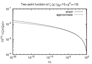
Fig. 2 shows the two-point function of for the same parameter choice, . The solid line is the exact correlation function calculated from Eqs. (39) and (42). The dashed line represents the approximated correlation function given by Eq. (47) in which second and higher order terms in are dropped. Here, we have assumed which appears in . This is because is roughly equal to the Hubble scale at the end of inflation for the massless preheating case with and taking to be the size of the present Universe we have . At , becomes as large as and it monotonically decreases to at . The current observations can probe the primordial fluctuation from the current Horizon scale down to the several order of magnitude smaller than it. This leads to the huge hierarchy . For such an observationally relevant range, given by Eq. (12) becomes mildly smaller than unity (typically ). Although is suppressed only mildly in this case, in order to capture the basic point of our result in analytic way, we regard as the expansion parameter and Taylor-expand the correlators with respect to it as can be seen in Fig. 2.
It is interesting to consider the meaning of the first term on the R. H. S. of Eq. (47). Using the definition of given by Eq. (45), we have
| (48) |
We now introduce a Gaussian window function defined by
| (49) |
This satisfies the normalization condition and effectively cuts off contributions from . With the Gaussian window function, can be written as
| (50) |
On the other hand, we can define #8#8 #8 This quantity was computed numerically in [42, 20] to estimate the resulting curvature perturbation on super-horizon scales. which is defined as a smoothed in the region by
| (51) |
We can verify that is related to the first derivative of evaluated at , namely,
| (52) |
Therefore, we can rewrite Eq. (47) as
| (53) |
This result shows that even when the original e-folding number is spiky and cannot be approximated as linear expression of the scalar field at all, at the leading order in the two-point function of is given by the first derivative of the e-folding number, just like the standard formula, provided it is smoothed over the range . As we will see later, this correspondence holds for the three-point function and even for the -point function of a general function (at leading order in ).
4.3 Non-Gaussianity
It is a straightforward and standard calculation to perform the three-dimensional integral of Eq. (9) for given by Eq. (38). However, since the resulting expression is complex and long, we write down the expression after applying the approximation as what we did for the case of the two-point function. The result is given by
| (54) |
where and are defined by
| (55) | |||||
| (56) | |||||
where . In the regime where , the three-point function of is
| (57) | |||||
where is defined by
| (58) |
Interestingly, the last equation takes the same form as Eq. (19), i. e. , the three-point function of at physically relevant scales becomes the standard local type one common to many models such as curvaton model and the modulated reheating one. The corresponding is given by
| (59) |
In the same way as we derived Eq. (50), we can write and in terms of the Gaussian window function as
| (60) |
We can show that the second derivative of defined by Eq. (51) is given by
| (61) |
Then, we have
| (62) |
Therefore, is also given by the standard expression based on the formalism provided the e-folding number is understood as the smoothed one over the region #9#9 #9 By adopting values of and provided by [20], this fact was used in [21] to compute from the massless preheating..
Given the current situation where cosmic measurements turn out to be useful to probe the four-point function, or trispectrum (for instance, see [46]), it is intriguing to go one step further from the three point function and to evaluate the four-point function. The calculation is tedious but straightforward. Again with the approximations that and , we find that the four-point function reduces to
| (63) | |||||
where
| (64) |
We see that the four-point function is contributed by two distinct parts. Indeed, this is exactly the same form as the standard local type four-point function which is parametrically represented as
| (65) | |||||
where and are non-linearity parameters for the four-point function [23]. Comparing this with Eq. (63), we can read
| (66) |
Our results show that the non-linearity parameters are given by the combination of the moments . Each moment can be numerically evaluated provided position , amplitude and width of each spike are known, which we will carry out in a following way. But before going to the numerical results, we can make a crude numerical estimate of the non-linearity parameters. From the figure in [20], for the relevant range of , we find that and and spikes. As is clear from the expression of (see Eq. (45)), only the spikes having contribute to and we have . Similarly, we expect . On the other hand, since terms in the summation of are either positive or negative with the (almost) equal probability, they may partially cancel out each other. As a result, we would expect is at most . Therefore, unless accidental cancellation to have occurs, as a crude estimation, we have . Similar consideration yields . As we will see below, this estimation indeed provides the correct orders of magnitude of the non-linearity parameters.

With the same parameters, we performed realizations of the mock and calculated and for each realization. Fig. 3 shows the resultant distribution of the non-linearity parameters plotted in logarithmic scale for fixed parameters . Since both and can be positive or negative, the distributions are shown for each quadrant defined for plane. We see that the distribution is highly concentrated in the region specified by and , which roughly agrees with our earlier analytic estimation. Also, we see a clear tendency that larger entails larger . We also find that the distribution is wide and covers a several orders of magnitude. The large is realized when becomes much tinier compared to and due to the accidental cancellation among terms in the summation given by Eq. (45). Since both and have in their denominators, generically becomes large as well when large is realized. Actually, the distribution for higher lies on a line , which supports the explanation due to the cancellation of . The opposite case in which accidentally happens is also possible and becomes small in such a case. Since the numerator of , which is given by , is independent of that of , the vanishing of does not result in the vanishing of in general, which explains the disappearance of the positive correlation that exists for higher . This consideration suggests that, in principle, either of any very large (and ) or very small can be realized after we perform sufficiently large number of realizations. In other words, we can say that the non-linearity parameters are quite sensitive to the realizations of . This would imply that the (slightly) imperfect modelling of has a possibility of leading to a significant error on the estimation of the resulting non-linearity parameters. Just for illustration, in Figs. 5 and 5, we show two different due to the different realizations with the same parameters . These correspond to the extreme cases where for the former case and for the latter. It is easy to recognise that they have the similar feature but different in detail, but not easy, without implementing the numerical calculations, to say if they produce quite different or not.


Very large corresponding to right-hand region of Fig. 3 should be taken with caveat. As we mentioned earlier, such very huge is realized when becomes tiny. In such a case, the higher order terms in appearing in the correlation functions, which are neglected as being subdominant, are no longer suppressed. In order to clarify this point more quantitatively, let us extend the expansion of Eqs. (47) and (57) to one more higher order;
| (67) | |||||
| (68) | |||||
We find from the first equation that the higher order terms become important if we have . In terms of , we can rewrite this condition as . Therefore, if becomes larger than , the standard expression of the three-point function written as the two product of the two-point functions, which is given by Eq. (19), loses its validity and the use of the constant to characterize the strength of non-Gaussianity becomes pointless. In stead of the standard relation, in the limit , we have
| (69) |
Thus the three-point function is completely determined by the two-point function without unknown parameter.
We also study how the non-linearity parameters vary as we shift for a fixed generated randomly (one realization). Fig. 6 shows the result in which is varied from to with the condition . As we can see, becomes quite tiny (and even becomes zero) at some specific values of . also does, but at different values of , which is expected because of the reasoning we made earlier. We also observe that is significantly enhanced (and even diverge) at some specific values of for which is also amplified as well. This can be again understood as the accidental vanishing of due to the cancellation of terms entering the summation of . Although this is for one realization, we checked that the qualitative feature remains the same for other realizations. Thus, it is a general consequence that we have and for most of the values of , but they happen to become either tiny or huge if is suitably fine-tuned.

To summarize our findings, we have two sources of the uncertainties that deaden the predictability of the model on the non-linearity parameters. The first one is due to the incomplete imitation of the mock . As we have seen, two mock that look similar occasionally yield quite different values of and with some small probability. This issue may be, in principle, resolved by knowing the correct form of the real precisely, which is beyond the scope of this paper. Furthermore, even if we know the correct form of , it is not clear of whether the Gaussian fitting given by Eq. (37), which is essential in the sense that it allows analytic study of the correlation functions to some extent, is approximate enough to derive the reliable values of the non-linearity parameters. This is a difficult problem and we do not pursue it in this paper. Instead, we take a conservative stance that our approach can only estimate the likely values of and .
The second uncertainty is due to the indeterminacy of , which is more fundamental than the first one. Since is a statistical quantity reflecting the large wavelength modes outside the box size, it is impossible in principle to predict a definite value of . As a result, we cannot predict the values of and , although it may be allowed to say at least that and are likely to happen.
4.4 Consistency check of the mock mapping
So far, our study is done with the mock mappings which are not the ones obtained by the lattice calculations. It is therefore interesting to compare the results based on the mock mappings with the ones based on the lattice calculations. Since we do not have the original numerical data of , we have read off the coordinates of out of the Fig. 1 presented in [20] by using the public software. In order to extract the position, height and width of each spike, we smoothed the obtained by the Gaussian window function with a width which is smaller than but is large enough to eliminate the fine spikes. Fig. 8 shows the resultant smoothed graph. Height of each spike is a little bit smaller than the original one given in [20], which is caused by the smoothing. The width is, instead, more broadened to compensate the loss of the height. From this data, we extract the position, height and width of each spike. We set the minimum height of spike we count in the analysis to be . We choose this value to avoid the inclusion of small spikes which appear to deviate from normal distribution function.


Fixing and , we can calculate the moments by using the Eqs. (45) and so on. Fig. 8 shows the dependence of on with by using the formula (59). We see that Fig. 8 looks quite similar to Fig. 6 in a sense that is typically but accidentally becomes very small or large for some particular values of . This supports that our findings derived in the previous section by using the mock mappings capture the essential part and are not modified significantly by the use of the real mapping.
4.5 Observational consequences
So far, our analysis is based on the assumption that the total curvature perturbation originates from preheating. This cannot describe the primordial perturbation of our Universe since the produced curvature perturbation from preheating does not have enough amplitude to explain the observed amplitude. Assuming and corresponding to as typical values, we have from Eq. (47). At the Sachs-Wolfe region corresponding to low in the CMB multipole , the curvature perturbation is related to the CMB temperature anisotropy by , where is the CMB mean temperature. Using the WMAP observations which detect of the power of the temperature fluctuations [17], we find is required from observations. This is about four orders of magnitude larger than that from preheating, which is observed in Fig. 2. Therefore, we need additional perturbations that account for the dominant part of the total curvature perturbations. Let us assume that the standard adiabatic perturbation from inflation plays this role. With this assumption, the total curvature perturbation is a mixture of two contributions, which can be written as
| (70) |
It should be now understood that all the calculations done in the previous subsections are for . It is known that the single field inflation with the canonical kinetic term predicts deviation of from Gaussianity is suppressed by the slow-roll parameters. If the Lagrangian of the inflaton field is more complex or there are multiple fields responsible for inflation, non-Gaussianity of can be boosted up to observable level in general (see for instance [8] and references therein.). In this section, we assume that is Gaussian just for simplicity. From the requirement that explains the observed amplitude of the CMB temperature anisotropy, we have
| (71) |
Therefore, to fit this with the observed slope of the two-point function (spectral index) is achieved simply by picking up the suitable inflaton potential. Dynamics of preheating does not enter this game. On the other hand, from the Gaussianity ansatz for , we also have
| (72) |
In the region where the lowest order approximation given by Eq. (57) works well, Eq. (72) can be written as
| (73) |
where is defined by
| (74) |
and represents the relative contribution of the curvature perturbation of the preheating origin to the total two-point function. By definition, we have . Strictly speaking, is a function of (although its dependence on is logarithmic) and the factorization of Eq. (74) is mathematically inconsistent. Nonetheless, this factorization is still useful to estimate the magnitude of the three-point function if it is observationally important or not. Taking and as representative values, a typical value of is estimated as . Comparison of Eq. (73) with Eq. (19) enables us to define the effective given by
| (75) |
Choosing to be , we see that the effective gets smaller than the original one, for instance, shown in Figs. 3 and 6, by a small number . Interestingly enough, while the original is too large to be compatible with the existing observational constraint except for the cases in which is fine-tuned to some specific values, the suppression by the factor makes the effective to be typically in the range #10#10 #10 The general relativistic second order effects produce . Such effects are not considered in this paper. , which is below the detectable amplitude by observations. One may wonder if one can boost to much higher value than by making be accidentally small. However, this is not so since in the mixed case is proportional to rather than to . Thus, smaller results in smaller and is the robust upper bound on in the massless preheating of our case.
In a similar way, the four-point function can be written as
| (76) | |||||
Correspondingly, the non-linearity parameters are given by
| (77) |
Thus, is enhanced by compared with . Actually, is always larger than or equal to irrespective of the underlying model [47, 48, 49]. Particularly, as the above equation shows, enhancement of compared to is the general feature for the case where the curvature perturbation is a mixture of the dominating Gaussian perturbation and the sub-dominant non-Gaussian perturbation [50, 51]. In light of the situation that Planck satellite can constrain to be up to [52], observational studies of trispectrum can be quite useful to examine if the trace of preheating is left in the non-Gaussianity of the curvature perturbation. The second equation of (77) shows that we may expect to be . This is a several orders of magnitude smaller than the sensitivity expected to be accomplished in future observations [53], but is still larger by a few orders of magnitude than the one coming from the standard adiabatic fluctuation .
5 General cases
Here, we have seen that, for the curvature perturbations sourced by preheating, three-point and four-point functions at the leading order in take exactly the same forms as those of the standard local type non-Gaussianity for which the curvature perturbation is given by the expansion of as
| (78) |
at the leading order in . In this section, we will show that this is not the special property limited to the curvature perturbations from preheating, but the generic feature of any curvature perturbation given by Eq. (3), for which expansion in terms of needs not to be a good approximation, provided obeys Gaussian statistics. Thus, the only assumption we will make in this section is that is small enough to allow us to pick up the leading terms in any correlator of . We will thus leave the function form of unspecified.
In the present situation, we can Taylor-expand Eq. (9) in terms of truncate it at the leading order. Thus the resultant expression consists of terms, each of which contains the product of . Each fully connected term in the correlator, which we are interested in, corresponds to the product such that any appears at least once in the argument of and a corresponding diagram, which has -vertices to each of which is attached without duplication and is constructed by drawing line between and if we have in , is simply connected. For instance, appearing in the four-point function does not give the connected term, while does. At the leading order in , corresponding connected diagrams are tree diagrams, which do not have any loop inside, because any connected loop diagram is made by attaching lines to some connected tree diagram with the same number of vertices, which is accompanied by additional powers of . It turns out that any connected tree diagram having -vertices has internal lines. This means that any leading connected term in the -point function of contains a product of ’s. Therefore, at the leading order in , we have
| (79) |
where means we take only connected parts of . As mentioned above, we can associate each term in Eq. (79) with the corresponding connected diagram. Since all the possible combinations in the product of ’s appear in Eq. (79), all the possible connected tree diagrams contribute to Eq. (79). Since the connected tree diagrams having -vertices that are not isomorphic to each other show different scale dependence due to different appearance of the combination of the product of . The number of connected tree diagrams is equal to that of the independent parameters required to parametrize the -point function. This is exactly the same property for the -point function of the standard local type curvature perturbation of the form (78) at the tree level [54, 55]. Therefore, Eq. (79) has exactly the same structure as the one for the standard local type curvature perturbation.
Conversely, from a given connected tree diagram, we can construct a corresponding non-linearity parameter contributing to Eq. (79) according to a following rule. For a vertex to which a vector is attached, we assign , where is a number of lines coming out of the vertex. Without a loss of generality, we can assume . For a line connecting the vertices and , we assign . We then multiply all of them and integrate it over , which gives one term in Eq. (79). In order to make things simpler, let us define the moments by
| (80) |
A connected tree diagram having -vertices can be characterized by a sequence consisting of integers . Therefore, a non-linearity parameter associated with the corresponding diagram can be written as
| (81) |
As illustrations, let us consider the three-point function. There is only one connected tree diagram with three vertices characterized by . Then, the non-linearity parameter can be written as
| (82) |
It can be explicitly verified that this equation exactly recovers Eq. (59) for the preheating case. In a similar way, for the four-point function, there are two connected tree diagrams characterized by and . The former case gives given by
| (83) |
The latter case give given by
| (84) |
This also coincides with Eq. (66) for the preheating case.
Finally, let us show that just as in the case for massless preheating in the last section, is related to the -th derivative of the smoothed e-folding number. The Fourier transform of the Gaussian window function defined by Eq. (49) can be written as
| (85) |
With this Fourier-transformed window function, we can write the smoothed e-folding number as
| (86) |
Thus, its -th derivative becomes
| (87) |
where we have used Eq. (80) in the last equation. This shows that, to compute the correlation function of , we can apply the standard diagrammatic rule following from the formalism, namely to assign -th derivative of the e-folding number to the vertex where lines are attached, simply by replacing the bare e-folding number with the smoothed e-folding number.
6 Conclusion
There are some inflationary models where the resultant curvature perturbation is a function of the Gaussian scalar field but its dependence cannot be approximated by quadratic expression. Representative models include the trigonometric mapping and the massless preheating models. In this paper, we provided a general formulation to calculate the correlation functions of the curvature perturbation which is an arbitrary function of the Gaussian scalar field . The -point function of the curvature perturbation is written as -dimensional integral, which can be evaluated once the Fourier transform of the mapping between and field is given. We applied the formalism first to the common local type non-Gaussian curvature perturbation and verified that it reproduces the standard local form of the three-point function. We then considered more non-trivial cases including the model in which the curvature perturbation is the trigonometric function of the scalar field. Due to the appearance of the Dirac’s -function, this model allows analytic evaluation of the correlation function.
By using the fitting formula provided in [20] which approximates each spike of the mapping as the normal distribution function, we could analytically perform the integrals for the two-point, three-point and four-point functions of . For physically relevant scales, forms of the correlation functions reduce to the standard local type ones. In particular, while the non-linearity parameters defining the strength of the non-Gaussianity of are related to the derivatives of the e-folding number with respect to in the standard case, the role of the derivatives is replaced by the moments defined as sums over spikes with suitable weights for the case of preheating, or equivalently, by the derivatives of the e-folding number smoothed in the field space. Due to the lack of the knowledge of the precise positions of the spikes and their widths and amplitudes, we randomly generated the mapping of mock ’s having the similar properties to the original one found in [20] and studied how the resultant non-linearity parameters differ according to different realizations. We found that the non-linearity parameters take naively estimated values for most of the realizations but some realizations yield very large or small values due to occasional cancellation among contributions from each spike. Even after the parameters appearing in the original Lagrangian are fixed, statistical indeterminacy of the average value of in our observable universe also causes another uncertainty of the non-linearity parameters. We therefore studied dependence of the non-linearity parameters on the average value of for a fixed realization. It was found that for some specific values (these values differ by different realizations) the non-linearity parameters are sharply enhanced or diminished compared to the naively estimated values. These analyses show that we can only estimate the likely values (order of magnitude) of the non-linearity parameters.
Due to the insufficient amplitude of the curvature perturbation from preheating, the curvature perturbation in our observable universe, if the massless preheating indeed happened in the early universe, must be a mixture of another dominant component and the subdominant one of preheating origin. Assuming the dominant component to be the standard adiabatic Gaussian perturbation coming from inflaton, the mixture reduces the non-Gaussianity of the total curvature perturbation to the observationally allowed range. The trispectrum is relatively amplified compared to the bispectrum and use of both observables will be useful to search preheating signature buried in the curvature perturbation.
By a diagrammatic approach,
we also showed that when the correlation function of can be treated
perturbatively, the forms of the correlation functions of
coincide with the standard local type ones at the leading order approximation.
While the non-linearity parameters are given by the product of the derivatives of the e-folding number
in the standard case,
they are given exactly the same manner even in our case provided we replace the bare e-folding
number with the one smoothed in the field space with a Gaussian window function.
Diagrammatic rule for converting the diagram to the corresponding non-linearity
parameter was also provided.
Acknowledgments: The authors thank to Masahiro Kawasaki and Jun’ichi Yokoyama for helpful discussions. We also thank to Liyi Gu for suggesting the use of the public software which extracts data from graphs. TS thanks the Leung Center for Cosmology and Particle Astrophysics (LeCosPA), National Taiwan University for the kind hospitality during his visit when this paper is completed. This work was supported by Grant-in-Aid for JSPS Fellows No. 1008477 (TS) and No. 24-2775(SY).
References
- [1] David Lyth and Andrew Liddle. The primordial density perturbation. Cambridge University Press, 2009.
- [2] Andrei D. Linde and Viatcheslav F. Mukhanov. Nongaussian isocurvature perturbations from inflation. Phys.Rev., D56:535–539, 1997.
- [3] Kari Enqvist and Martin S. Sloth. Adiabatic CMB perturbations in pre - big bang string cosmology. Nucl.Phys., B626:395–409, 2002.
- [4] David H. Lyth and David Wands. Generating the curvature perturbation without an inflaton. Phys.Lett., B524:5–14, 2002.
- [5] Takeo Moroi and Tomo Takahashi. Effects of cosmological moduli fields on cosmic microwave background. Phys.Lett., B522:215–221, 2001.
- [6] Gia Dvali, Andrei Gruzinov, and Matias Zaldarriaga. A new mechanism for generating density perturbations from inflation. Phys.Rev., D69:023505, 2004.
- [7] Lev Kofman. Probing string theory with modulated cosmological fluctuations. 2003.
- [8] E. Komatsu, N. Afshordi, N. Bartolo, D. Baumann, J.R. Bond, et al. Non-Gaussianity as a Probe of the Physics of the Primordial Universe and the Astrophysics of the Low Redshift Universe. 2009.
- [9] Teruaki Suyama, Tomo Takahashi, Masahide Yamaguchi, and Shuichiro Yokoyama. On Classification of Models of Large Local-Type Non-Gaussianity. JCAP, 1012:030, 2010.
- [10] Alexei A. Starobinsky. Multicomponent de Sitter (Inflationary) Stages and the Generation of Perturbations. JETP Lett., 42:152–155, 1985.
- [11] D.S. Salopek and J.R. Bond. Nonlinear evolution of long wavelength metric fluctuations in inflationary models. Phys.Rev., D42:3936–3962, 1990.
- [12] Misao Sasaki and Ewan D. Stewart. A General analytic formula for the spectral index of the density perturbations produced during inflation. Prog.Theor.Phys., 95:71–78, 1996.
- [13] Misao Sasaki and Takahiro Tanaka. Superhorizon scale dynamics of multiscalar inflation. Prog.Theor.Phys., 99:763–782, 1998.
- [14] David H. Lyth, Karim A. Malik, and Misao Sasaki. A General proof of the conservation of the curvature perturbation. JCAP, 0505:004, 2005.
- [15] David H. Lyth and Yeinzon Rodriguez. The Inflationary prediction for primordial non-Gaussianity. Phys.Rev.Lett., 95:121302, 2005.
- [16] Eiichiro Komatsu and David N. Spergel. Acoustic signatures in the primary microwave background bispectrum. Phys.Rev., D63:063002, 2001.
- [17] C.L. Bennett, D. Larson, J.L. Weiland, N. Jarosik, G. Hinshaw, et al. Nine-Year Wilkinson Microwave Anisotropy Probe (WMAP) Observations: Final Maps and Results. 2012.
- [18] Tomislav Prokopec and Thomas G. Roos. Lattice study of classical inflaton decay. Phys.Rev., D55:3768–3775, 1997.
- [19] Patrick B. Greene, Lev Kofman, Andrei D. Linde, and Alexei A. Starobinsky. Structure of resonance in preheating after inflation. Phys.Rev., D56:6175–6192, 1997.
- [20] J. Richard Bond, Andrei V. Frolov, Zhiqi Huang, and Lev Kofman. Non-Gaussian Spikes from Chaotic Billiards in Inflation Preheating. Phys.Rev.Lett., 103:071301, 2009.
- [21] Kazunori Kohri, David H. Lyth, and Cesar A. Valenzuela-Toledo. Preheating and the non-gaussianity of the curvature perturbation. JCAP, 1002:023, 2010.
- [22] David Middleton. An Introduction to Statistical Communication Theory. McGRAW-HILL BOOK COMPANY, INC., 1960.
- [23] Christian T. Byrnes, Misao Sasaki, and David Wands. The primordial trispectrum from inflation. Phys.Rev., D74:123519, 2006.
- [24] Kazuhiro Yamamoto, Michiyasu Nagasawa, Misao Sasaki, Hiroshi Suzuki, and Jun’ichi Yokoyama. Statistics of baryon isocurvature perturbations in the inflationary universe. Phys.Rev., D46:4206–4217, 1992.
- [25] Bruce A. Bassett, Shinji Tsujikawa, and David Wands. Inflation dynamics and reheating. Rev.Mod.Phys., 78:537–589, 2006.
- [26] Jennie H. Traschen and Robert H. Brandenberger. Particle production during out-of-equilibrium phase transitions. Phys.Rev., D42:2491–2504, 1990.
- [27] Lev Kofman, Andrei D. Linde, and Alexei A. Starobinsky. Reheating after inflation. Phys.Rev.Lett., 73:3195–3198, 1994.
- [28] Lev Kofman, Andrei D. Linde, and Alexei A. Starobinsky. Towards the theory of reheating after inflation. Phys.Rev., D56:3258–3295, 1997.
- [29] Bruce A. Bassett and Fermin Viniegra. Massless metric preheating. Phys.Rev., D62:043507, 2000.
- [30] F. Finelli and Robert H. Brandenberger. Parametric amplification of metric fluctuations during reheating in two field models. Phys.Rev., D62:083502, 2000.
- [31] Bruce A. Bassett, Fabrizio Tamburini, David I. Kaiser, and Roy Maartens. Metric preheating and limitations of linearized gravity. 2. Nucl.Phys., B561:188–240, 1999.
- [32] Shinji Tsujikawa, Bruce A. Bassett, and Fermin Viniegra. Multifield fermionic preheating. JHEP, 0008:019, 2000.
- [33] J.P. Zibin, Robert H. Brandenberger, and Douglas Scott. Back reaction and the parametric resonance of cosmological fluctuations. Phys.Rev., D63:043511, 2001.
- [34] Shinji Tsujikawa and Bruce A. Bassett. When can preheating affect the CMB? Phys.Lett., B536:9–17, 2002.
- [35] Yasusada Nambu and Yohei Araki. Evolution of non-linear fluctuations in preheating after inflation. Class.Quant.Grav., 23:511–526, 2006.
- [36] Mar Bastero-Gil, Matthieu Tristram, Juan Francisco Macias-Perez, and D. Santos. Non-linear Preheating with Scalar Metric Perturbations. Phys.Rev., D77:023520, 2008.
- [37] Kari Enqvist, Asko Jokinen, Anupam Mazumdar, Tuomas Multamaki, and Antti Vaihkonen. Non-Gaussianity from instant and tachyonic preheating. JCAP, 0503:010, 2005.
- [38] Kari Enqvist, Asko Jokinen, Anupam Mazumdar, Tuomas Multamaki, and Antti Vaihkonen. Cosmological constraints on string scale and coupling arising from tachyonic instability. JHEP, 0508:084, 2005.
- [39] Dhiraj Kumar Hazra, Jerome Martin, and L. Sriramkumar. The scalar bi-spectrum during preheating in single field inflationary models. Phys.Rev., D86:063523, 2012.
- [40] Asko Jokinen and Anupam Mazumdar. Very large primordial non-gaussianity from multi-field: application to massless preheating. JCAP, 0604:003, 2006.
- [41] Takahiro Tanaka and Bruce Bassett. Application of the separate universe approach to preheating. astro-ph/0302544.
- [42] Teruaki Suyama and Shuichiro Yokoyama. Generating the primordial curvature perturbations in preheating. Class.Quant.Grav., 24:1615–1626, 2007.
- [43] Alex Chambers and Arttu Rajantie. Lattice calculation of non-Gaussianity from preheating. Phys.Rev.Lett., 100:041302, 2008.
- [44] Alex Chambers and Arttu Rajantie. Non-Gaussianity from massless preheating. JCAP, 0808:002, 2008.
- [45] Andrei V. Frolov. DEFROST: A New Code for Simulating Preheating after Inflation. JCAP, 0811:009, 2008.
- [46] Eiichiro Komatsu. Hunting for Primordial Non-Gaussianity in the Cosmic Microwave Background. Class.Quant.Grav., 27:124010, 2010.
- [47] Teruaki Suyama and Masahide Yamaguchi. Non-Gaussianity in the modulated reheating scenario. Phys.Rev., D77:023505, 2008.
- [48] Kendrick M. Smith, Marilena LoVerde, and Matias Zaldarriaga. A universal bound on N-point correlations from inflation. Phys.Rev.Lett., 107:191301, 2011.
- [49] Naonori S. Sugiyama. Consistency Relation for multifield inflation scenario with all loop contributions. JCAP, 1205:032, 2012.
- [50] Kazuhide Ichikawa, Teruaki Suyama, Tomo Takahashi, and Masahide Yamaguchi. Non-Gaussianity, Spectral Index and Tensor Modes in Mixed Inflaton and Curvaton Models. Phys.Rev., D78:023513, 2008.
- [51] Kazuhide Ichikawa, Teruaki Suyama, Tomo Takahashi, and Masahide Yamaguchi. Primordial Curvature Fluctuation and Its Non-Gaussianity in Models with Modulated Reheating. Phys.Rev., D78:063545, 2008.
- [52] Noriyuki Kogo and Eiichiro Komatsu. Angular trispectrum of cmb temperature anisotropy from primordial non-gaussianity with the full radiation transfer function. Phys.Rev., D73:083007, 2006.
- [53] Joseph Smidt, Alexandre Amblard, Christian T. Byrnes, Asantha Cooray, Alan Heavens, et al. CMB Constraints on Primordial non-Gaussianity from the Bispectrum () and Trispectrum ( and ) and a New Consistency Test of Single-Field Inflation. Phys.Rev., D81:123007, 2010.
- [54] Christian T. Byrnes, Kazuya Koyama, Misao Sasaki, and David Wands. Diagrammatic approach to non-Gaussianity from inflation. JCAP, 0711:027, 2007.
- [55] Shuichiro Yokoyama, Teruaki Suyama, and Takahiro Tanaka. Efficient diagrammatic computation method for higher order correlation functions of local type primordial curvature perturbations. JCAP, 0902:012, 2009.