Dirac Kirchhoff diffraction theory

The time-independent Helmholtz equation can be derived from the stationary Schrödinger equation as well as the optical wave equation for the scalar electric field $E$. In what follows, the quantum mechanical notation of $\Psi$ is used, to ease the transition to Dirac spinors. The static wave equation for an eigenstate $\Psi$ with energy $E=\frac{\hbar^{2}k^{2}}{2m}$ is given by:

This is the static Helmholtz equation. Setting the right-hand side to $-\delta(\boldsymbol{r}-\boldsymbol{r}^{\prime})$, and keeping the part of the solution that satisfies Sommerfeld’s radiation condition [14], gives following Green’s function:

By using the Gauss-Ostrogradski theorem, one can derive Green’s theorem [15],

Where $U_{1}$ and $U_{2}$ are two scalar functions that will be filled in shortly, $V$ is a closed volume with bordering surface $S$, and vectors $\boldsymbol{r}_{S}$ lie on that surface. Filling in $U_{1}=\Psi(\boldsymbol{r})$ (a solution of (1)) and $U_{2}=G(\boldsymbol{r},\boldsymbol{r}^{\prime})$ into (3), one can obtain the Helmholtz-Kirchhoff integration theorem:

This equation gives an exact solution to the wave equation (1) in any point $\boldsymbol{r}^{\prime}$ of $V$, given the value of $\Psi(\boldsymbol{r}_{S})$ on the bordering surface $S$. Being a fundamental result of a physically implied Helmholtz equation and the mathematically rigorous Gauss-Ostrogradski theorem, it finds applications in many fields of physics (albeit in a more general form). The above can be seen as the mathematical basis of cosmologist’s holographic principle [16]: information encoded on a (hyper)surface completely defines the internal state inside the entire volume enclosed by that surface.

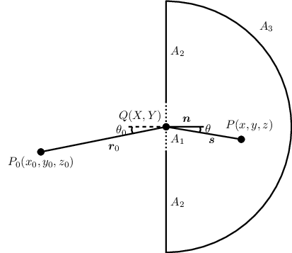
The mathematical model of the diffraction setup is shown in fig. 1. A point source is located at $P_{0}$ at distance $r_{0}$ from an aperture $A_{1}$. At point $Q\in A_{1}$, light can be transmitted into the right bounded volume which contains a screen at $P$ at a distance $s$ from the aperture. We will now calculate the disturbance at point $P$ caused by the point source $P_{0}$. $A_{3}$ is a surface that mathematically goes to infinity. The boundary conditions used by Kirchhoff are:

• •

  $\Psi(\boldsymbol{r})=\partial_{\boldsymbol{r}}\Psi(\boldsymbol{r})=0$ on $A_{2}$ and $A_{3}$,

• •

  $\Psi(\boldsymbol{r})=\frac{e^{ik\boldsymbol{r}}}{\boldsymbol{r}}$ on $A_{1}$, i.e. for $\boldsymbol{r}=\boldsymbol{r}_{0}$, which represents a field originating in a point source $P_{0}$ which illuminates the aperture.

Note it is the first of above conditions that breaks down mathematically; for an analytic function that has both its value and its derivate $0$ on a finite region, it must be zero everywhere, which cannot be physically true. Rayleigh-Sommerfeld diffraction theory sets only one to zero, resulting in two solutions that are mathematically sound. The problem is choosing the correct boundary conditions. In reality, the Kirchhoff approximation produces very useful results nonetheless, to a high degree of accuracy in the approximations assumed here.
Some additional approximations are necessary to get a useful result: we let $kr_{0}\gg 1$ and $ks\gg 1$, which means that both the source and focal plane are far away from the aperture, reducing wavefront curvature effects which take more care to be included. This leads to the Kirchhoff-Fresnel diffraction formula:

This is valid directly behind the aperture. The quantity $\frac{\cos{\theta_{0}}+\cos{\theta}}{2}$ is called the obliquity factor. $\theta_{0}\approx 0$ is valid for a point source far away from the aperture, and $\theta\approx 0$ amounts to a small angle far field approximation. The far field approximations and their near field improvements are discussed extensively in optics literature [17], and not of primary interest here. For completeness, the Fraunhofer diffraction formula that one can derive by applying these approximations to (5) can be written as follows:

with $P=(k_{x},k_{y})$ a point in the focal plane (given in Fourier space, which can simply be rescaled to represent real coordinates in that plane), $(X,Y)$ are the coordinates on the aperture, and $\Psi_{\text{Ap}}$ is the wave function in the aperture. This formula states that one can easily calculate the far-field image (including not only density but also phase) if one knows the wave function in the aperture. Also note that this theory applies equally well to photon waves (described by the wave equation which is fully relativistically applicable) and the Schrödinger equation (which applies to non-relativistic matter waves).
In what follows, the derivation done by P. Hillion [10, 11] in light of the 2-component spinor electromagnetic field is expanded to the full 4-component spinor Dirac theory for massive particles with spin.

The Dirac equation for spin-$\frac{1}{2}$ particles is:

which is relativistically covariant, and in most common usage a 4-component matrix equation for the Dirac spinor $\Psi$. Applying the complex conjugate Dirac operator to the Dirac equation gives an interesting and well-known result:

where $\eta^{\nu\mu}$ is the Minkowski metric of spacetime. The above is nothing less than the scalar Klein-Gordon equation for every component of the Dirac spinor independently. This property will be used in the following section. In a stationary situation, one can write $\Psi(\boldsymbol{r},t)\propto\Psi(\boldsymbol{r})e^{-iEt}$, which results in

One can now define a new variable, $k^{2}=m^{2}+E^{2}$, which leads to a familiar form:

The stationary Dirac equation can now be rewritten using this new variable as

without loss of generality.

Using the fact that the solutions of the Dirac equation form a subset of those of the Klein-Gordon equation, one can construct a solution to the Dirac equation $\Psi$ from scalar solutions of the Klein-Gordon equation $\psi^{\mu}$:

This is a well-known fact. As an extension, which is also used by Hillion [11], one can construct a Green’s matrix solution to

from the scalar Green’s function (2) as follows:

which is a useful form used in the next section.

In this section, a 4-component spinor analogue of the Helmholtz-Kirchhoff integration theorem (4) is derived from the Dirac equation. Multiplying (7) with $g(\boldsymbol{r},\boldsymbol{r}^{\prime})$ on the left and subtracting that from (13) multiplied on the right by $\Psi(\boldsymbol{r})$, one has:

By using the correct mathematical formulation, one can easily prove that the Gauss-Ostrogradski theorem also applies to spinor objects [11, 18], in which case one can integrate (15) over a volume $V$ around the point $\boldsymbol{r}^{\prime}$ and write:

where the integration is over the closed surface $S$ around $V$, containing all the vectors $\boldsymbol{r}_{S}$. $\gamma^{n}$ is the compound $\gamma$ matrix perpendicular to the surface. Obviously a $\gamma$ matrix cannot be perpendicular to a surface, and this is a purely notational convenience. An example of $\gamma^{n}$ can easily be given in the case of a spherical surface, namely $\gamma^{r}=\sin{\theta}\cos{\phi}\gamma^{1}+\sin{\theta}\sin{\phi}\gamma^{2}+\cos{\theta}\gamma^{3}$, which is nothing more that the vector transformation to spherical coordinates. It is not surprising the $\gamma$ matrices transform as vectors, as they are the basis vectors of the Dirac algebra. This makes $\gamma^{n}$ more than only “notational convenience”, and a mathematical $\gamma$ object can easily be seen as orthogonal to a surface. From (2) one can prove

This expression can be used to rewrite (16) into a form comparable to (4):

The next steps are exactly the same as in the scalar theory: Kirchhoff’s boundary conditions and approximations are applied, along with:

• •

  $\gamma^{r}\approx\gamma^{3}$: when the beam is directed along the $z$ axis, $\gamma^{r}$ coincides with $\gamma^{3}$,

• •

  $\partial_{r_{0}}s\approx-1$: valid for calculations almost directly behind the aperture.

gives the spinor Kirchhoff-Fresnel diffraction formula (compare with (5)):

One can again perform the exact same approximations as in the scalar case to reduce (19), leading to a similar form as in (6):

which gives the Dirac spinor form for the far-field image of a diffracted $z$-oriented beam.

The advantage of working in the Dirac representation is the simplicity of its non-relativistic limit. Taking the limit $\frac{\boldsymbol{k}}{E+m}\rightarrow 0$, it is readily known only the top two components of the Dirac spinor contribute, and the $\gamma$-factor effectively reduces to a negligible scaling operation for a spin eigenstate. By this, the formula (20) reduces simply to the classical form (6) in the non-relativistic case.

The theory derived here highlights the simple fact that for diffraction through a scalar aperture of a paraxial relativistic fermion beam, spin is conserved. This is made clear by the $\gamma$ factor which is multiplied with the incoming spinor, mixing only the large and small components of the same spin elements, the explicit form for the $z$-direction given below for the Dirac representation:

For the other directions, the nonzero elements of the $\gamma$-factor align with the nonzero elements of the plane wave spinor with its spin aligned in that direction. For example, the spinor part of a plane wave eigenstate of $\Sigma_{z}=+1$ is given by

which, after multiplication with $(1+\gamma^{3})\gamma^{3}$, is still in the same eigenstate of $\Sigma_{z}$. The Fourier transform will not affect the spinor structure. Hence, the far field spinor given by (20) is also unmodified with respect to spin after diffraction. This result implies that a pure diffraction experiment with a scalar aperture will not be influenced by electron spin, at least in the paraxial region. Some mixing may occur far from the beam axis, where $\left(1+\gamma^{r}\right)\gamma^{r}$ is not well approximated by (for the $z$ direction) $\left(1+\gamma^{3}\right)\gamma^{3}$. The generality of the results derived here allow to extend the simple approximation (20) to more complicated scenarios, including any type of spin polarization.

It is well known that Kirchhoff’s boundary conditions lead to physical solutions containing a grave mathematical inconsistency. By putting both the wave function and its derivative to zero on a finite region of space, one has inevitably that $\Psi$, an analytic function, must be zero everywhere inside the bounding surface (this includes all points $P$). Rayleigh and Sommerfeld solved this by deriving two possible integration formulas, each for different boundary conditions: one has only the wavefunction zero, the other has only its derivative zero on the “dark areas”. Table 1 attempts to give an overview of the conceptual differences between the three integral formalisms.

The Kirchhoff-Helmholtz integration theorems for these cases under the present approximations differ slightly:

In the Dirac case, the Green’s functions become the Green’s matrices derived from the scalar Green’s functions, through (14). Note that one can also apply the conjugate Dirac operator in that equation, and the resulting Green’s matrix will be antisymmetric to the one used here (see [11]), which is expected from the anticommutator relationship fullfilled by the Dirac spinors.

References

- [1] F. Hénault, J. Opt. Soc. Am. A 27, 435 (2010).
- [2] M. Takeda, H. Ina, and S. Kobayashi, J. Opt. Soc. Am. 72, 156 (1982).
- [3] M. Takeda and K. Mutoh, Appl. Opt. 22, 3977 (1983).
- [4] J. Verbeeck, H. Tian, and P. Schattschneider, Nature 467, 301 (2010).
- [5] J. Verbeeck, H. Tian, and A. Béché, Ultramicroscopy 113, 83 (2012).
- [6] P. Schattschneider, M. Stg̈er-Pollach, S. Löffler, A. Steiger-Thirsfeld, J. Hell, and J. Verbeeck, Ultramicroscopy 115, 21 (2012).
- [7] K. Y. Bliokh, Y. P. Bliokh, S. Savel’ev, and F. Nori, Phys. Rev. Lett. 99, 190404 (2007).
- [8] P. Schattschneider and J. Verbeeck, Ultramicroscopy 111, 1461 (2011).
- [9] L. Janicijevic and S. Topuzoski, J. Opt. Soc. Am. A 25, 2659 (2008).
- [10] P. Hillion and S. Quinnez, Journal of Optics 14, 143 (1983).
- [11] P. Hillion, Journal of Mathematical Physics 19, 264 (1978).
- [12] P. Hillion, Journal of Optics 10, 21 (1979).
- [13] P. Hillion and S. Quinnez, Journal of Optics 18, 51 (1987).
- [14] A. Sommerfeld, Partial Differential Equations in Physics (Academic Press, 1949).
- [15] G. B. Arfken, H. J. Weber, and F. E. Harris, Mathematical Methods for Physicists, 6th ed. (Elsevier Academic Press, 2005) pp. 60–63.
- [16] G. F. Smoot, International Journal of Modern Physics D 19, 2247 (2010).
- [17] E. Hecht, Optics (Fourth Edition) (Addison Wesley, 2002).
- [18] H. Jeffreys and B. Swirles, Methods of Mathematical Physics, third edition (University Press, 1972).