Cavity Optomechanics
Abstract
We review the field of cavity optomechanics, which explores the interaction between electromagnetic radiation and nano- or micromechanical motion. This review covers the basics of optical cavities and mechanical resonators, their mutual optomechanical interaction mediated by the radiation pressure force, the large variety of experimental systems which exhibit this interaction, optical measurements of mechanical motion, dynamical backaction amplification and cooling, nonlinear dynamics, multimode optomechanics, and proposals for future cavity quantum optomechanics experiments. In addition, we describe the perspectives for fundamental quantum physics and for possible applications of optomechanical devices.
I Introduction
Light carries momentum which gives rise to radiation pressure forces. These forces were already postulated in the 17th century by Kepler, who noted that the dust tails of comets point away from the sun during a comet transit [207]. The first unambiguous experimental demonstrations of the radiation pressure force predicted by Maxwell were performed using a light mill configuration [292, 232]. A careful analysis of these experiments was required to distinguish the phenomenon from thermal effects that had dominated earlier observations. As early as 1909, Einstein derived the statistics of the radiation pressure force fluctuations acting on a moveable mirror [124], including the frictional effects of the radiation force, and this analysis allowed him to reveal the dual wave-particle nature of blackbody radiation. In pioneering experiments, both the linear and angular momentum transfer of photons to atoms and macroscopic objects were demonstrated by Frisch [138] and by Beth [31], respectively.
In the 1970s Arthur Ashkin demonstrated that focused lasers beams can be used to trap and control dielectric particles, which also included feedback cooling [18, 19]. The non-conservative nature of the radiation pressure force and the resulting possibility to use it for cooling atomic motion was first pointed out by Hänsch and Schawlow and by Dehmelt and Wineland [164, 424]. Laser cooling was subsequently realized experimentally in the 1980s and has become since then an extraordinarily important technique [374]. It has, for example, allowed cooling of ions to their motional ground state and it is the underlying resource for ultracold atom experiments. Many applications have been enabled by laser cooling [275], including optical atomic clocks, precision measurements of the gravitational field, and systematic studies of quantum many-body physics in trapped clouds of atoms [41].
The role of radiation pressure and its ability to provide cooling for larger objects was already investigated earlier by Braginsky in the context of interferometers. Braginsky considered the dynamical influence of radiation pressure on a harmonically suspended end-mirror of a cavity. His analysis revealed that the retarded nature of the force, due to the finite cavity lifetime, provides either damping or anti-damping of mechanical motion, two effects that he was able to demonstrate in pioneering experiments using a microwave cavity [53, 55]. In later experiments, these phenomena were also observed in microwave-coupled -scale mechanical resonators [106]. Independently, similar physics was explored theoretically for solid-state vibrations [119]. In the optical domain, the first cavity optomechanical experiment [117] demonstrated bistability of the radiation pressure force acting on a macroscopic end-mirror.
Braginsky also addressed the fundamental consequences of the quantum fluctuations of radiation pressure and demonstrated that they impose a limit on how accurately the position of a free test mass (e.g. a mirror) can be measured [54, 52]. A detailed analysis by Caves clarified the role of this ponderomotive quantum noise in interferometers [74]. These works established the standard quantum limit for continuous position detection, which is essential for gravitational wave detectors such as LIGO or VIRGO.
During the 1990s, several aspects of quantum cavity optomechanical systems started to be explored theoretically. These include squeezing of light [128, 259] and quantum non-demolition (QND) detection of the light intensity [188, 314], which exploit the effective Kerr nonlinearity generated by the optomechanical interaction. It was also pointed out that for extremely strong optomechanical coupling the resulting quantum nonlinearities could give rise to nonclassical and entangled states of the light field and the mechanics [258, 45]. Furthermore, feedback cooling by radiation pressure was suggested [260]. Around the same time, in a parallel development, cavity-assisted laser-cooling was proposed as a method to cool the motion of atoms and molecules that lack closed internal transitions [169, 408].
On the experimental side, optical feedback cooling based on the radiation pressure force was first demonstrated in [96] for the vibrational modes of a macroscopic end-mirror. This approach was later taken to much lower temperatures [215, 319]. At the same time, there was a trend to miniaturize the mechanical element. For example, the thermal motion of a -scale mirror was monitored in a cryogenic optical cavity [384]. Producing high-quality optical Fabry-Perot cavities below that scale, however, turned out to be very challenging. In spite of this, it was still possible to observe optomechanical effects of retarded radiation forces in microscale setups where the forces were of photothermal origin, effectively replacing the cavity lifetime with a thermal time constant. Examples include demonstration of the optical spring effect [407], feedback damping [274], self-induced oscillations [432, 178], and cavity cooling due to the dynamical backaction of retarded photothermal light forces [179].
Yet, for future applications in quantum coherent optomechanics it is highly desirable to be able to exploit the non-dissipative radiation pressure force. Both the advent of optical microcavities and of advanced nanofabrication techniques eventually allowed to enter this regime. In 2005 it was discovered that optical microtoroid resonators with their high optical finesse at the same time contain mechanical modes and thus are able to display optomechanical effects, in particular radiation-pressure induced self-oscillations [337, 72, 211] (i.e. the effect Braginsky termed ‘‘parametric instability’’11 1 Braginsky called the process of dynamical backaction amplification and the concomitant self-induced coherent oscillations “parametric oscillatory instability”, as this effect is undesirable in gravitational wave interferometers which were the basis of his analysis.). In 2006 three different teams demonstrated radiation-pressure cavity cooling, for suspended micromirrors [150, 13] and for microtoroids [359]. Since then, cavity optomechanics has advanced rapidly and optomechanical coupling has been reported in numerous novel systems. These include membranes [380] and nanorods [133] inside Fabry-Perot resonators, whispering gallery microdisks [417, 190] and microspheres [254, 300, 386], photonic crystals [120, 121], and evanescently coupled nanobeams [10]. In addition, cavity optomechanics has been demonstrated for the mechanical excitations of cold atom clouds [288, 62]. Optomechanical interactions are also present in optical waveguides - as first studied and observed in the context of squeezing, where the confined mechanical modes of fibers lead to Guided Acoustic Wave scattering [367]. Nowadays there are a number of systems where such optomechanical interactions are explored in the absence of a cavity, such as waveguides in photonic circuits or photonic crystal fibres, see e.g. [242, 201]. These setups lie somewhat outside the scope of the concepts presented in this review, but we emphasize that they are very promising for applications due to their large bandwidth.
Optomechanical coupling has also been realized using microfabricated superconducting resonators, by embedding a nanomechanical beam inside a superconducting transmission line microwave cavity [327] or by incorporating a flexible aluminum membrane into a lumped element superconducting resonator [379]. In these systems the mechanical motion capacitively couples to the microwave cavity. This approach ties cavity optomechanics to an independent development that has been garnering momentum since the late 1990s, which is concerned with measuring and controlling the motion of nano- and micromechanical oscillators using electrical and other non-optical coupling techniques. Examples include coupling of mechanical oscillators to single electron transistors [88, 225, 289] or a quantum point contact [88, 136]. Besides a wealth of possible applications for such devices in sensitive detection [90, 343, 226], these methods provide the possiblility of realizing mechanical quantum devices [364, 40, 126] by direct interaction with two-level quantum systems [89, 343, 423, 227, 297, 15, 222]. For recent comprehensive general reviews of nanomechanical systems (in particular electro-mechanical devices), we refer the reader to [40, 320, 154].
It should be noted that in atomic systems quantum coherent control of mechanical motion is state of the art since early pioneering experiments with trapped ions – for reviews see [236, 39, 193]. In fact, quantum information processing in these systems relies on using the quantum states of motion to mediate interactions between distant atomic spins [85]. In contrast, the fabricated nano- and micromechanical structures that form the subject of this review will extend this level of control to a different realm, of objects with large masses and of devices with a great flexibility in design and the possibility to integrate them in on-chip architectures.
There are several different motivations that drive the rapidly growing interest into cavity optomechanics. On the one side, there is the highly sensitive optical detection of small forces, displacements, masses, and accelerations. On the other hand, cavity quantum optomechanics promises to manipulate and detect mechanical motion in the quantum regime using light, creating nonclassical states of light and mechanical motion. These tools will form the basis for applications in quantum information processing, where optomechanical devices could serve as coherent light-matter interfaces, for example to interconvert information stored in solid-state qubits into flying photonic qubits. Another example is the ability to build hybrid quantum devices that combine otherwise incompatible degrees of freedoms of different physical systems. At the same time, it offers a route towards fundamental tests of quantum mechanics in an hitherto unaccessible parameter regime of size and mass.
A number of reviews [212, 213, 268, 131, 143, 21, 360, 98, 22, 279] and brief commentary papers [204, 87, 265, 97] on cavity optomechanics have been published during the past few years, and the topic has also been discussed as part of a larger reviews on nanomechanical systems [320, 154]. Here we aim for a comprehensive treatment that incorporates the most recent advances and points the way towards future challenges.
This review is organized follows: We first discuss optical cavities, mechanical resonators, the basic optomechanical interaction between them and the large range of experimental setups and parameters that are now available. We then go on to derive the basic consequences of the interaction (such as optomechanical damping and the optical spring effect), describe various measurement schemes, and present the quantum theory of optomechanical cooling. After studying nonlinear effects in the classical regime, we address multimode setups and the wide field of proposed applications in the quantum domain, before concluding with an outlook.
| Symbol | Meaning |
|---|---|
| Mechanical frequency | |
| Mechanical damping rate | |
| Mechanical quality factor, | |
| Laser detuning from the cavity resonance, | |
| Overall cavity intensity decay rate, from input coupling and intrinsic losses, . | |
| Optomechanical single-photon coupling strength, in | |
| Light-enhanced optomechanical coupling for the linearized regime, | |
| Optical frequency shift per displacement, | |
| Mechanical zero-point fluctuation amplitude, | |
| Photon annihilation operator, with the circulating photon number | |
| Phonon annihilation operator, with the phonon number | |
| Average number of phonons stored in the mechanical resonator, | |
| Average phonon number in thermal equilibrium, | |
| Photon number circulating inside the cavity, | |
| Optical susceptibility of the cavity, | |
| Mechanical susceptibility, | |
| Quantum noise spectrum, (Sec. II.2.3) | |
| (Symmetrized) mechanical zero-point fluctuations, | |
| : standard quantum limit result for added noise in displacement measurement (Sec. VI.1) | |
| Optomechanical damping rate (Sec. V.2.2): max. for | |
| Optical spring (mechanical frequency shift, Sec. V.2.1): for | |
| Minimum reachable phonon number in laser-cooling, for |
II Optical cavities and mechanical resonators
In this section we recall the basic aspects of optical cavities and of mechanical resonators, as needed to describe cavity optomechanical systems. Much more about these topics can be found in standard textbooks on quantum optics, e.g. [410], and on nanomechanical systems [91].
II.1 Optical resonators
Optical resonators can be realized experimentally in a multitude of forms of which several types will be discussed later in the review. Here we give a unifying description of the optical properties and provide the mathematical description of a cavity that is pumped with a single monochromatic laser source.
II.1.1 Basic properties
We first consider the classical response of a simple Fabry-Perot resonator, which will allow to introduce the relevant parameters to characterize an optical cavity. A Fabry-Perot resonator or etalon consisting of two highly reflective mirrors, separated by a distance , contains a series of resonances which are given by the angular frequency Here is the integer mode number. The separation of two longitudinal resonances is denoted as the free spectral range (FSR) of the cavity:
| (1) |
In the following, we will almost always focus on a single optical mode, whose frequency we will denote .
Both the finite mirror transparencies and the internal absorption or scattering out of the cavity lead to a finite photon (intensity) cavity decay rate22 2 In this review we shall use for the photon (energy) decay rate, such that the amplitude decay rate is given by . In some papers the latter is denoted as . .
A further useful quantity is the optical finesse, , which gives the average number of round-trips before a photon leaves the cavity:
| (2) |
The optical finesse is a useful parameter as it gives the enhancement of the circulating power over the power that is coupled into the resonator. Alternatively, we can introduce the quality factor of the optical resonator,
| (3) |
where is the photon lifetime. Note that the quality factor is also used to characterize the damping rate of mechanical resonators (see below). Generally speaking, the cavity decay rate can have two contributions, one from losses that are associated with the (useful) input (and output) coupling and a second contribution from the internal losses. It is useful to differentiate these two contributions. For the case of a high-Q cavity, the total cavity loss rate can be written as the sum of the individual contributions:
Here, refers to the loss rate associated with the input coupling, and refers to the remaining loss rate. For example, in the case of a waveguide coupled to a microtoroidal or microsphere resonator, is the loss rate associated with the waveguide-resonator interface and describes the light absorption inside the resonator. For the case of a Fabry-Perot cavity, is the loss rate at the input cavity mirror and summarizes the loss rate inside the cavity, including transmission losses at the second cavity mirror as well as all scattering and absorption losses behind the first mirror. Note that by splitting the total decay rate into these two contributions, we are assuming that the photons going into the decay channel will not be recorded. More generally, one could distinguish between more decay channels (e.g. input mirror, output mirror, absorption).
II.1.2 Input-output formalism for an optical cavity
A quantum mechanical description of a cavity that is coupled to the outside electromagnetic environment can be given either via master equations (if only the internal dynamics is of interest) or via a framework known as input-output theory, if one also wants to access the light field being emitted by (or reflected from) the cavity. Input-output theory allows us to directly model the quantum fluctuations injected from any coupling port (such as the input mirror) into the cavity. In addition, it takes into account any coherent laser drive that may be present. For more details beyond the brief discussion provided below, see e.g. [141, 93].

Input-output theory is formulated on the level of Heisenberg equations of motion, describing the time-evolution of the field amplitude inside the cavity. One finds that the amplitude experiences decay at a rate . At the same time, its fluctuations are constantly replenished via the quantum noise entering through the various ports of the cavity. In the present case, we distinguish between the channels associated with the input coupling (decay rate ) and the other loss processes (overall decay rate , including loss through the second mirror). The equation of motion reads:
| (4) |
In the classical case, would be replaced by a properly normalized complex amplitude of the electric field of the cavity mode under consideration. Indeed, the classical version of this equation (and the following ones) can be obtained by simply taking the average, such that . We have chosen a frame rotating with the laser frequency , i.e. and have introduced the laser detuning with respect to the cavity mode (see also Sec. III.2). Note that a similar equation can also be written down for the mechanical oscillator in order to describe its dissipation and the associated noise force, comprising quantum and thermal contributions (see Sec. III.3).
The input field should be thought of as a stochastic quantum field. In the simplest case, it represents the fluctuating vacuum electric field coupling to the cavity at time , plus a coherent laser drive. However, the same formalism can also be used to describe squeezed states and other more complex field states. The field is normalized in such a way that
is the input power launched into the cavity, i. e. is the rate of photons arriving at the cavity. The same kind of description holds for the “unwanted” channel associated with .
According to the input-output theory of open quantum systems, the field that is reflected from the Fabry Perot resonator (or coupled back into the coupling waveguide) is given by:
| (5) |
Note that this input-output relation describes correctly the field reflected from the input mirror of a Fabry-Perot resonator. The above equation describes also the transmitted pump field of an evanescently coupled uni-directional waveguide resonator system, such as a whispering gallery mode resonator coupled to a waveguide [69]. In this case the above expression would yield the transmitted pump field.
We still have to consider the case of a two-sided cavity, e.g. a two-sided Fabry Perot cavity. Other examples in this review include a waveguide coupled to superconducting stripline cavities or fiber-taper coupled photonic crystal defect cavities. In these cases there are both transmitted and reflected fields. In all of these cases there are two options for the description. If the field transmitted through the second mirror is not of interest to the analysis, one may lump the effects of that mirror into the decay rate , which now represents both internal losses and output coupling through the second mirror. If, however, the field is important, it should be represented by an additional term of the type in Eq. (4). Then an equation analogous to Eq. (5) will hold for the output field at that second mirror.
In the following, we will not be concerned with noise properties, but focus instead on classical average quantities (for a single-sided cavity), taking the average of Eqs. (4) and (5).
We can solve the equation (4) first for the steady-state amplitude in the presence of a monochromatic laser drive whose amplitude is given by . Noting that we obtain:
| (6) |
The expression linking the input field to the intracavity field will be referred to as the optical susceptibility,
Thus, the steady-state cavity population , i.e the average number of photons circulating inside the cavity, is given by:
| (7) |
were is the input power launched into the cavity. The reflection or transmission amplitude (for the case of a Fabry-Perot cavity or a waveguide-coupled resonator, respectively) can be calculated by inserting Eq. (6) into Eq. (5). Using the symbol for the reflection amplitude in the sense of figure 2 case (b), we obtain:
| (8) |
The square of this amplitude gives the probability of reflection from the cavity (for Fabry-Perot) or transmission in the case of a uni-directional waveguide resonator system. From this expression, several regimes can be differentiated. If the external coupling dominates the cavity losses (, the cavity is called “overcoupled”. In that case and the pump photons emerge from the cavity without having been absorbed or lost via the second mirror (a property that is important as discussed below in the context of quantum limited detection). The case where refers to the situation of “critical coupling”. In this case, on resonance. This implies the input power is either fully dissipated within the resonator or fully transmitted through the second mirror (in the case of a Fabry-Perot cavity with denoting the decay through the second mirror). The situation is referred to as “undercoupling” and is associated with cavity losses dominated by intrinsic losses. For many experiments this coupling condition is not advantageous, as it leads to an effective loss of information.
The physical meaning of reflection (or transmission) depends sensitively on the experimental realization under consideration. One can distinguish four scenarios, which are outlined in the figure 2.
II.2 Mechanical resonators
II.2.1 Mechanical normal modes
The vibrational modes of any object can be calculated by solving the equations of the linear theory of elasticity under the appropriate boundary conditions that are determined by the geometry33 3 A powerful simulation approach in this context are finite element (FEM) simulations. [91]. This eigenvalue problem yields a set of normal modes and corresponding eigenfrequencies . The mechanical displacement patterns associated with mechanical motion are given by the strain field where designates the normal mode.
For the purposes of this review, we will mostly focus on a single normal mode of vibration of frequency (where ’’ stands for ’mechanical’), assuming that the mode spectrum is sufficiently sparse such that there is no spectral overlap with other mechanical modes. The loss of mechanical energy is described by the (energy) damping rate which is related to the mechanical quality factor44 4 In the context of mechanical dissipation often the loss tangent is quoted, its relation to the quality factor being . by If one is interested in the equation of motion for the global amplitude of the motion, one can utilize a suitably normalized (see below) dimensionless mode function , such that the displacement field would be . Then the temporal evolution of can be described by the canonical simple equation of motion of a harmonic oscillator of effective mass :
| (9) |
Here denotes the sum of all forces that are acting on the mechanical oscillator. In the absence of any external forces, it is given by the thermal Langevin force (see Sec. II.2.3). In the above equation the (energy) damping rate has been assumed to be frequency independent. Deviations of this model are treated for example in [353].
A brief remark about the effective mass is necessary at this point [91, 315]. The normalization that has been chosen for the mode function affects the normalization of . However, it will always be true that the potential energy is given by . This value can then be compared to the expression for the potential energy that arises from a calculation according to the theory of elasticity. Demanding them to be equal yields the correct value for the effective mass (which therefore is seen to depend on the normalization that was chosen for the mode function). Of course, for the simple case of a center-of-mass oscillation of a solid object, a natural definition of is the center of mass displacement in which case the effective mass will be on the order of the total mass of the object. A treatment of effective mass in optomechanical experiments is found in [315].
Eq. (9) can be solved easily, which is best done in frequency space. We introduce the Fourier transform via . Then defines the susceptibility , connecting the external force to the response of the coordinate:
| (10) |
The low frequency response is given by where is the spring constant55 5 To describe the response of a high Q oscillator near resonance one can approximate by a Lorentzian, i.e. using yields .
The quantum mechanical treatment of the mechanical harmonic oscillator leads to the Hamiltonian
Here the phonon creation () and annihilation () operators have been introduced, with
where
is the zero-point fluctuation amplitude of the mechanical oscillator, i.e. the spread of the coordinate in the ground-state: , and where denotes the mechanical vacuum state. The position and momentum satisfy the commutator relation . The quantity is the phonon number operator, whose average is denoted by . In the following, we will typically not display explicitly the contribution of the zero-point energy to the energy of the oscillator.
We briefly discuss the effect of dissipation. If the mechanical oscillator is coupled to a high temperature bath, the average phonon number will evolve according to the expression:
For an oscillator which is initially in the ground state, this implies a simple time dependence of the occupation according to , where is the average phonon number of the environment. Consequently, the rate at which the mechanical oscillator heats out of the ground state is given by:
The latter is often referred to as the thermal decoherence rate, and given by the inverse time it takes for one quantum to enter from the environment. In the above expression the high temperature limit has been taken, i.e. This expression shows that to attain low decoherence a high mechanical Q factor and a low temperature bath are important. The change of population of a certain Fock state can be described within the framework of the Master equation approach. This approach allows to calculate the decoherence rate of other quantum states such as a Fock state . The latter is given by (see e.g.[141]):
revealing that higher Fock states exhibit a progressively higher rate of decoherence.
II.2.2 Mechanical dissipation
The loss of mechanical excitations, i.e. phonons, is quantified by the energy dissipation rate . The origins of mechanical dissipation have been intensively studied over the last decades and comprehensive reviews are found for example in [91, 126]. The most relevant loss mechanisms include:
- •
- •
- •
- •
materials-induced losses, which are caused by the relaxation of intrinsic or extrinsic defect states in the bulk or surface of the resonator [431, 284, 369, 397, 389]. Such losses have been successfully described by a phenomenological model involving two level defect states, which are coupled to the strain via the deformation potential [9, 309, 383, 186, 365, 328]. In the context of nano- and micromechanical oscillators the two level fluctuator damping has been revisited [365, 328].
The various dissipation processes contribute independently to the overall mechanical losses and hence add up incoherently. The resulting mechanical quality factor is given by , where labels the different loss mechanisms.
Another helpful quantity is the so-called “” product, which plays an important role in the phase noise performance of oscillators. In the context of optomechanics, it quantifies the decoupling of the mechanical resonator from a thermal environment. Specifically, , denotes the number of coherent oscillations in the presence of thermal decoherence, and evidently scales with .

II.2.3 Susceptibility, noise spectra and fluctuation dissipation theorem
If one measures the motion of a single harmonic oscillator in thermal equilibrium, one will observe a trajectory oscillating at the eigenfrequency . However, due to the influence of both mechanical damping and the fluctuating thermal Langevin force, these oscillations will have a randomly time-varying amplitude and phase. Both amplitude and phase change on the time scale given by the damping time . Such real-time measurements have been performed in optomechanical systems [159] (see Fig. 4).
In experiments, the mechanical motion is often not analyzed in real-time but instead as a noise spectrum in frequency space. This allows to easily separate the contributions from different normal modes. We briefly recapitulate the relevant concepts. Given one particular realization of the trajectory obtained during a measurement time , we define the gated Fourier transform over a finite time interval :
| (11) |
Averaging over independent experimental runs, we obtain the spectral density . In the limit , the Wiener-Khinchin theorem connects this to the Fourier transform of the autocorrelation function, also called the noise power spectral density:
| (12) |
Here we have defined:
| (13) |
The only assumption which has been made is that is a stationary random process. From Eqs. (12,13), we immediately obtain the important result that the area under the experimentally measured mechanical noise spectrum yields the variance of the mechanical displacement, :
| (14) |
Furthermore, in thermal equilibrium, the fluctuation-dissipation theorem (FDT) relates the noise to the dissipative part of the linear response,
| (15) |
where denotes the mechanical susceptibility introduced above and we have treated the high-temperature (classical) case. For weak damping (), this gives rise to Lorentzian peaks of width in the noise spectrum, located at (see Fig. 5). Integration of according to Eq. (14) yields the variance, which for weak damping is set by the equipartition theorem: .
In the quantum regime, the natural generalization of Eq. (13) contains the product of Heisenberg time-evolved operators, , which do not commute. As a consequence, the spectrum is asymmetric in frequency. The quantum FDT
| (16) |
implies that for at . Our discussion of dynamical backaction cooling will mention that this means the bath is not able to supply energy, as there are no thermal excitations. In this review we will also consider the symmetrized noise spectrum, . For more on noise spectra, we refer to [93].
III Principles of optomechanical coupling
III.1 The radiation pressure force and optomechanical coupling
In our discussion the fundamental mechanism that couples the properties of the cavity radiation field to the mechanical motion is the momentum transfer of photons, i.e. radiation pressure. The simplest form of radiation pressure coupling is the momentum transfer due to reflection that occurs in a Fabry Perot cavity. A single photon transfers the momentum (: photon wavelength). As a consequence the radiation pressure force is given by
Here denotes the cavity round trip time. Therefore, describes the radiation pressure force caused by one intracavity photon. The parameter which appears in this expression describes also the change of cavity resonance frequency with position, i.e. the frequency pull parameter. In the next section, which introduces a Hamiltonian description of the interaction between a movable mirror and optical cavity, this relation will be derived in its full generality.
More generally, the optomechanical coupling can arise for example by direct momentum transfer via reflection (Fabry-Perot type cavities with a moveable end-mirror, microtoroids), by coupling via a dispersive shift of the cavity frequency (membrane in the middle, levitated nano-objects trapped inside the cavity) or by optical near-field effects (e.g. nano-objects in the evanescent field of a resonator or a waveguide just above a substrate).
Various radiation pressure forces have been investigated in the pioneering work of Ashkin, who first demonstrated that small dielectric particles can be trapped in laser light [19]. The relevant forces are generally referred to as gradient (or dipole) forces, as the force arises from the gradient of the laser field intensity. The particle is attracted to the center of the Gaussian trapping laser beam. If denotes the laser electric field distribution, the time-averaged dielectric energy of the particle in the field is given by (with the polarizability) which correspondingly yields a force In addition to the gradient force, scattering forces occur for a traveling wave. These forces scale with , i.e. the wavenumber of the electromagnetic radiation, in contrast to the gradient forces. In addition there is also a contribution from the strain-optical effect, i.e. the strain-dependent polarizability. The strain-optical coupling is the dominant coupling mechanism in guided acoustic wave scattering [367, 248]. Independent of the physical interpretation of the force, however, the optomechanical interaction in an optomechanical system can always be derived by considering the cavity resonance frequency shift as a function of displacement (i.e. the “dispersive” shift). This will be the basis for our Hamiltonian description adopted in the next section.
It is important to note at this point that a significant difference between the trapping of particles in free space and micromechanical systems is the fact that the latter are also subject to radiation forces based on thermal effects. Absorption of light can heat a structure and deform it, which corresponds to the action of a force (e.g. in an asymmetric, bimorph structure, including materials of different thermal expansion). These photothermal forces can in many ways lead to effects similar to retarded radiation pressure forces, with the thermal relaxation time of the structure replacing the cavity photon lifetime. However, since such forces are based on absorption of light, they cannot form the basis for future fully coherent quantum optomechanical setups, since at least the coherence of the light field is thereby irretrievably lost.
III.2 Hamiltonian formulation
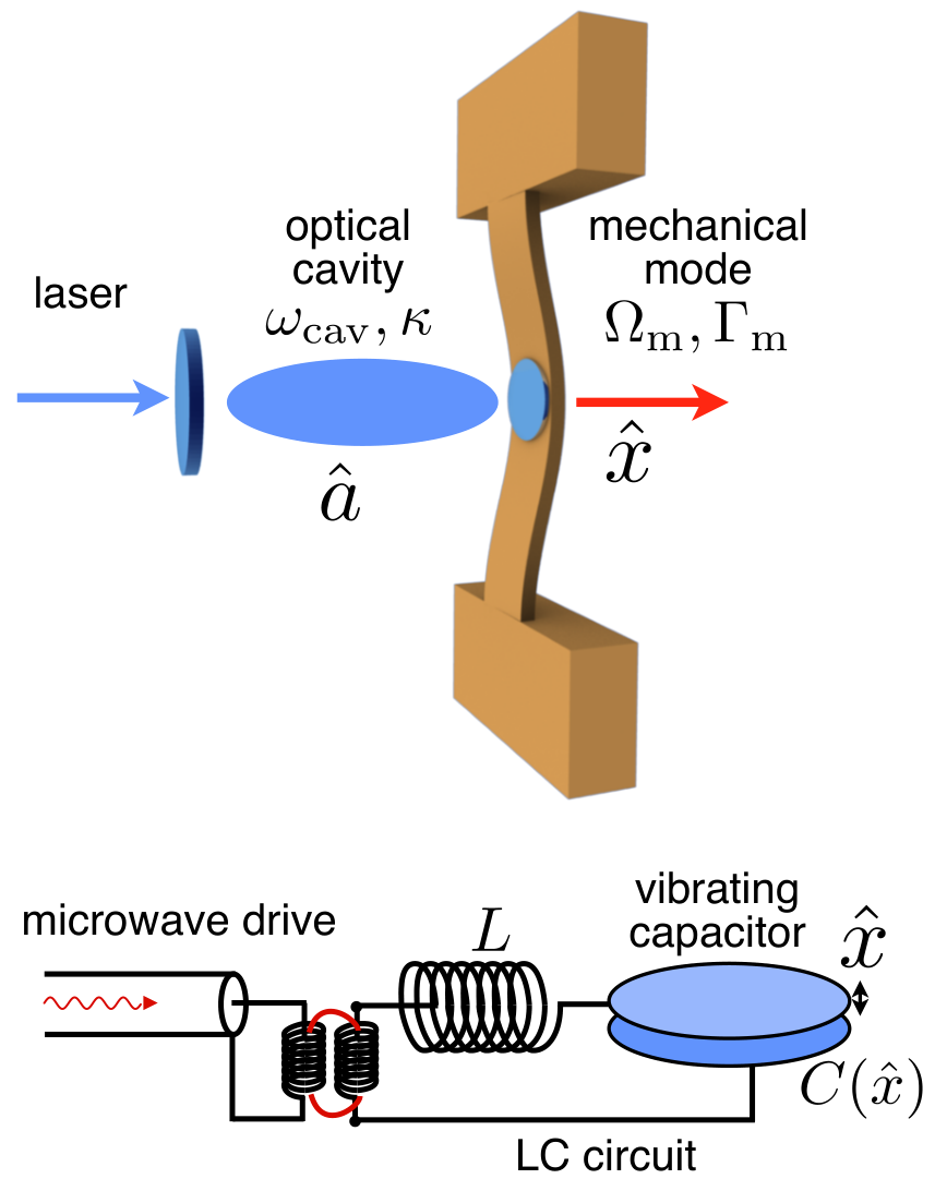
The starting point of all our subsequent discussions will be the Hamiltonian describing the coupled system of a radiation mode interacting with a vibrational mode (Fig. 1). For brevity we will refer to the radiation field as “optical”, even though the important case of microwave setups is included here as well.
We will focus here on the simplest possible model system in cavity optomechanics, which has been used to successfully describe most of the experiments to date. In this model, we restrict our attention to one of the many optical modes, i.e. the one closest to resonance with the driving laser. Moreover, we also describe only one of the many mechanical normal modes. This is mostly arbitrary, as the displacement frequency spectrum will show peaks at any of the mechanical resonances. Still, as long as the dynamics is linear with independently evolving normal modes, the model will provide a valid approximation. In some cases, like sideband-resolved cooling, it may be possible to experimentally select a particular mechanical mode by adjusting the laser detuning, whereas in other cases, like nonlinear dynamics, an extended description involving several mechanical modes may become crucial.
The uncoupled optical () and mechanical () mode are represented by two harmonic oscillators, which is typically an excellent approximation at the displacements generated in the experiments:
| (17) |
In the case of a cavity with a movable end mirror the coupling of optical and mechanical mode is parametric, i.e. the cavity resonance frequency is modulated by the mechanical amplitude66 6 Note that such a setup is also considered for discussions of the dynamical Casimir effect, where cavity photons are created by the mechanical modulation of the boundaries. In the optomechanical scenarios considered here, however, the mechanical frequencies are too small for this effect to play a role.:
For most experimental realizations discussed in this review, it suffices to keep the linear term, where we define the optical frequency shift per displacement as (but see Sec. VI.2.2 for another example). A more detailed derivation of the optomechanical Hamiltonian can be found in an early paper [231].
We mention in passing that other coupling mechanisms have been discussed. For example, the transparency of a moving Bragg mirror, and hence , can depend on its velocity [205]. More generally, the displacement may couple to the cavity decay rate, yielding . This case (sometimes termed “dissipative coupling”), which is of practical relevance in some setups [241], can lead to novel physical effects, e.g. in cooling [127].
For a simple cavity of length , we have . The sign reflects the fact that we take to indicate an increase in cavity length, leading to a decrease in if . In general, expanding to leading order in the displacement, we have:
| (18) |
Here , as defined before. Thus, the interaction part of the Hamiltonian can be written
| (19) |
where
| (20) |
is the vacuum optomechanical coupling strength, expressed as a frequency. It quantifies the interaction between a single phonon and a single photon. We stress that, generally speaking, is more fundamental than , since is affected by the definition of the displacement that is to some extent arbitrary for more complicated mechanical normal modes (see the discussion in Sec. II.2.1). Therefore, in the following we will almost always refer to . Further below, we will also mention , which is an often-used measure for the effective optomechanical coupling in the linearized regime. It will be enhanced compared to by the amplitude of the photon field. The Hamiltonian reveals that the interaction of a movable mirror with the radiation field is fundamentally a nonlinear process, involving three operators (three wave mixing).
The radiation pressure force is simply the derivative of with respect to displacement:
| (21) |
The full Hamiltonian will also include terms that describe dissipation (photon decay and mechanical friction), fluctuations (influx of thermal phonons), and driving by an external laser. These effects are formulated most efficiently using the equations of motion and the input-output formalism (see Sec. II.1.2, and also the next section). Here, we just remark that it is convenient to change the description of the optical mode by switching to a frame rotating at the laser frequency . Applying the unitary transformation makes the driving terms time-independent77 7 , and generates a new Hamiltonian of the form
| (22) |
where
| (23) |
is the laser detuning introduced already in Sec. II.1.2, and where we have omitted () driving, decay, and fluctuation terms, which will be discussed below. Eq. (22) is the frequently used starting point in cavity optomechanics.
We now introduce the so-called “linearized” approximate description of cavity optomechanics. To this end, we split the cavity field into an average coherent amplitude and a fluctuating term:
| (24) |
Then, the interaction part of the Hamiltonian
| (25) |
may be expanded in powers of . The first term, , indicates the presence of an average radiation pressure force . It may be omitted after implementing an appropriate shift of the displacement’s origin by . The second term, of order , is the one we keep:
| (26) |
The third term, , is omitted as being smaller by a factor . Without loss of generality, we will now assume real-valued. Thus, the Hamiltonian in the rotating frame reads
| (27) |
where the quadratic interaction part
| (28) |
is referred to as “linearized”, since the resulting coupled equations of motion will be linear in this approximation. Note that the remaining terms in Eq. (27) no longer contain the laser driving, as that has already been taken care of by the shift implemented in Eq. (24). In the literature up to now, the combination
| (29) |
is often referred to as “the optomechanical coupling strength”. Obviously, it depends on the laser intensity and is thus less fundamental than the single-photon coupling (obtained for ). In the linearized regime described here, the optomechanical system can be viewed in analogy to a linear amplifier [47] that receives optical and mechanical input fields.
The linearized description can be good even if the average photon number circulating inside the cavity is not large. This is because the mechanical system may not be able to resolve the individual photons if the decay rate is sufficiently large. The detailed conditions for the linearized approximation to be valid may depend on the questions that are asked. We will return to this question in the section on nonlinear quantum optomechanics (Sec. X.6).
We briefly note that is one neccessary condition for the so-called “strong coupling” regime of cavity optomechanics, where the mechanical oscillator and the driven optical mode hybridize (Sec. VII.2). A much more challenging condition is to have , i.e. the single-photon optomechanical coupling rate exceeding the cavity decay rate. In the latter regime, nonlinear quantum effects will become observable (see Sec. X.6).
Depending on the detuning, three different regimes can be distinguished with respect to the interaction (28), especially in the sideband-resolved regime (, which we assume in the remainder of this section). For , we have two harmonic oscillators of (nearly) equal frequency that can interchange quanta: the mechanical oscillator and the driven cavity mode. Within the rotating-wave approximation (RWA) we thus can write the interaction as
| (30) |
This is the case relevant for cooling (transferring all thermal phonons into the cold photon mode; Sec. VII.1) and for quantum state transfer between light and mechanics (Sec. X). In the quantum-optical domain, it is referred to as a “beam-splitter” interaction.
For , the dominant terms in RWA
| (31) |
represent a “two-mode squeezing” interaction that lies at the heart of parametric amplification [93]. In the absence of dissipation, this would lead to an exponential growth of the energies stored both in the vibrational mode and the driven optical mode, with strong quantum correlations between the two. Thus, it may be used for efficiently entangling both modes (Sec. X). Focussing on the mechanical mode alone, the growth of energy can be interpreted as “anti-damping” or amplification (Sec. V.2.2). If the intrinsic dissipation is low enough, this behaviour may trigger a dynamical instability that leads to self-induced mechanical oscillations. The resulting features will be discussed in Sec. VIII.
Finally, when , the interaction
| (32) |
means that the mechanical position leads to a phase shift of the light field, which is the situation encountered in optomechanical displacement detection (Sec. VI). In addition, this interaction Hamiltonian can be viewed as implementing QND detection of the optical amplitude quadrature , since that operator commutes with the full Hamiltonian in this case.
III.3 Optomechanical equations of motion
The mechanical motion induces a shift of the optical resonance frequency, which in turn results in a change of circulating light intensity and, therefore, of the radiation pressure force acting on the motion. This kind of feedback loop is known as optomechanical “backaction”. The finite cavity decay rate introduces some retardation between the motion and the resulting changes of the force, hence the term “dynamical” backaction.
A convenient starting point for the analytical treatment of the radiation-pressure dynamical backaction phenomena (Sec. V.2 and Sec. VII) is the input-output formalism. This formalism (briefly introduced in Sec. II.1.2) provides us with equations of motion for the cavity field amplitude and, analogously, for the mechanical amplitude . These equations have the form of Quantum Langevin equations88 8 In the standard approximation adopted here, these equations are Markoffian, i.e. without memory and with delta-correlated noise., since both the light amplitude and the mechanical motion are driven by noise terms that comprise the vacuum noise and any thermal noise entering the system:
| (33) | ||||
| (34) |
Please see Sec. II.1.2 for remarks on the input-output treatment and the optical decay rates . With regard to the damping term for the mechanical dissipation, we note that this treatment is correct as long as . Otherwise the equations would have to be formulated on the level of the displacement , with a damping force .
The noise correlators associated with the input fluctuations are given by:
| (35) | ||||
| (36) | ||||
| (37) | ||||
| (38) |
Here we have assumed that the optical field has zero thermal occupation (), which is an approximation that is valid for optical fields at room temperature, although it may fail for the case of microwave fields, unless the setup is cooled to sufficiently low temperatures. In contrast, the mechanical degree of freedom is typically coupled to a hot environment, with an average number of quanta given by . Together with these correlators, the quantum Langevin equations describe the evolution of the optical cavity field and the mechanical oscillator, including all fluctuation effects.
It is equally useful to give the classical, averaged version of these equations that will be valid for sufficiently large photon and phonon numbers, in the semiclassical limit. Then, we can write down the equations for the complex light amplitude and the oscillator position :
| (39) | ||||
| (40) |
Here we have neglected all fluctuations, although these could be added to describe thermal and even, in a semiclassical approximation, quantum noise forces. The term represents the laser drive. Note that we have also chosen to write the mechanical equation of motion in terms of the displacement, where . This becomes equivalent to the equation given above only for weak damping, . These fully nonlinear coupled differential equations will be the basis for our discussion of nonlinear phenomena, in particular the optomechanical parametric instability (also called “self-induced oscillations” or “mechanical lasing”, Sec. VIII).
The equations of motion Eq. (33), (34) (and likewise their classical versions) are inherently nonlinear as they contain the product of the mechanical oscillator amplitude and the cavity field (first line) or the radiation pressure force that is quadratic in photon operators (second line). While they can still be solved numerically in the classical case, for the quantum regime they are of purely formal use and in practice cannot be solved exactly, neither analytically nor numerically. However, in many situations that we will encounter it is permissible to linearize this set of equations around some steady-state solution: . Using and keeping only the linear terms, we find the following set of coupled linear equations of motion:
| (41) | ||||
| (42) | ||||
| (43) |
These correspond to what one would have obtained alternatively by employing the “linearized” coupling Hamiltonian of Eq. (28) and then applying input-output theory. Here we have (as is common practice) redefined the origin of the mechanical oscillations to take into account the constant displacement that is induced by the average radiation pressure force. It is evident that now the mutual coupling terms between the optical and mechanical degrees of freedom are linear in the field operators, and that the strength is set by the field-enhanced coupling rate .
As shown in the later sections, these linearized equations are able to fully describe several phenomena, including optomechanical cooling, amplification, and parametric normal mode splitting (i.e. strong, coherent coupling). They can be solved analytically, which is best performed in the frequency domain (see Sec. V.2).
For completeness, we display the linearized quantum equations in frequency space:
| (44) | ||||
| (45) |
Here is the Fourier transform of . Note the important relation , which has to be taken care of while solving the equations.
It is equally useful to consider the linearized version of the classical equations of motion for the light amplitude and the displacement, Eqs. (39) and (40):
| (46) | ||||
| (47) |
Finally, we display them in frequency space, in the form that we will employ in Sec. V.2.
| (48) | ||||
| (49) | ||||
Again, note .
IV Experimental realizations and optomechanical parameters
The increasing availability of high-quality optomechanical devices, i.e. high-Q mechanical resonators that are efficiently coupled to high-Q optical cavities, has been driving a plethora of experiments during the last years that are successfully demonstrating the working principles of cavity optomechanics. We now discuss some of the most frequently used architectures.

IV.1 Optomechanical parameters
The following table summarizes the relevant optomechanical parameters for some typical current experimental implementations. These are: the mechanical resonator frequency and mass ; the fundamental mechanical (phonon) and optical (photon) dissipation rates and , respectively; the “” product, which is a direct measure for the degree of decoupling from the thermal environment (specifically, is the condition for neglecting thermal decoherence over one mechanical period); the sideband suppression factor that determines the ability to realize ground-state cooling (see Sec.VII); and finally the bare optomechanical coupling rate , which corresponds to the cavity frequency shift upon excitation of a single phonon.
| Reference | [Hz] | [kg] | [Hz] | [Hz] | [Hz] | [Hz] | |
|---|---|---|---|---|---|---|---|
| [288] | 15.7 | ||||||
| [78] | 0.13 | ||||||
| [377] | 0.02 | ||||||
| [399] | 0.09 | ||||||
| [380] | |||||||
| [218] | 55 | ||||||
| [155] | |||||||
| [13] | |||||||
| [106] | 1.85 | 0.9 |
Some parameter combinations are of particular relevance for optomechanical tasks. The following figures provide an overview of the state of the art in current experiments. The data is compiled from published experiments. These are labelled as follows:
1 [106], 2 [272], 3 [327], 4 [333], 5 [377], 6 [78], 7 [142], 8 [380, 351], 9 [419], 10 [190], 11 [245], 12 [417], 13 [120], 14 [109], 15 [300], 16 [361], 17 [399], 18 [358], 19 [14], 20 [132], 21 [150], 22 [156], 23 [217], 24 [285], 25 [218], 26 [155], 27 [355], 28 [288], 29 [62], 30 [152], 31 [400]. Different symbols indicate the different optomechanical implementations: suspended mirrors (), optical microresonators (), photonic crystal cavities (), suspended nanoobjects (), microwave resonators (), cold atoms ().

IV.2 Suspended mirrors
An obvious way to realize optomechanical interactions in a cavity is to suspend one of the cavity’s mirrors. The mechanical motion changes directly the cavity length and hence the frequency response of such a ‘‘rubber cavity’’99 9 for the origin of this terminology see the Acknowledgements section of [45].
The first experimental implementations of this type were a Fabry-Perot cavity with moving mirrors and date back to the early attempts of laser interferometeric detection of gravitational waves [3]. While there the purpose of suspending the macroscopic cavity mirrors is to achieve acoustic isolation, optomechanical effects, in particular quantum mechanical radiation pressure fluctuations, eventually pose the fundamental limit for its interferometric sensitivity [74, 388] (see Section VI.1 for a detailed discussion). At the same time this configuration allows to exploit cavity optomechanics for the center of mass motion of truly macroscopic test masses. Experiments of that type have to date resulted in the demonstration of the optical bistability [117] (Sec. V.1), of the optical spring effect [366, 102] (Sec. V.2.1) and of optical cooling [103, 285] (Secs. V.2, VII) with suspended mirrors on the gram scale and even of feedback cooling of suspended mirrors on the kilogram scale at the LIGO facility [1]. A practical challenge of these experiments is their operation at very low mechanical frequencies (1 kHz), which requires sophisticated isolation against acoustic noise. For such experiments this is achieved by suspending the macroscopic mirrors over several stages. To minimize mechanical losses it has recently been suggested to levitate the macrosopic mirror in an optical trap [368]. Finally, this kind of setup also allows to monitor and to optomechanically control internal mechanical modes of macroscopic mirrors [96, 159], which are a dominant source for unwanted cavity phase noise e.g. in gravitational wave detectors [167, 166], in cavity QED [66] or in frequency stabilization of atomic optical clocks [294].
Another possibility is to use highly reflecting micromechanical devices as a Fabry-Perot end mirror. These systems include coated cantilevers [384, 179, 13, 16] and micropillars [402], micrometer-sized mirror pads on top of cantilevers [217, 132, 156, 218], or micromechanically suspended optical coatings [42, 99, 100] and photonic crystal slabs [12, 206]. Efficient optomechanical coupling in this configuration requires the size of the mechanical structure to be much larger than the wavelength of the light: typical cavity lengths range from to , with an optical finesse up to , which is generally limited by losses due to the finite cavity mirror sizes. It has been pointed out that additional interference effects may be able to overcome this limit significantly [216]. Compared to the macroscopic mirrors discussed above, these micromechanical devices allow access to higher mechanical frequencies (up to some tens of MHz) and, in principle, to higher mechanical quality factors. In particular, the possibility of exact geometric control via microfabrication techniques allows to minimize mechanical losses due to clamping [420, 11, 101].
The accessible mass and frequency ranges in combination with the restrictions on cavity length () and achievable cavity finesse set some practical limitations for this geometry. In particular, sideband-resolution (small ) and large optomechanical coupling (small , leading to a large ) impose conflicting conditions and need to be traded against each other. On the other hand, along with the macroscopic microwave transducers (see Sec.IV.6), this realization provides optomechanical control over by far the largest range of mass and frequency.
IV.3 Optical microresonators
A situation similar to the Fabry-Perot case occurs in optical microresonators, where light is guided in whispering gallery modes along the rim of a circular resonator [394]. There is a large number of different mechanical normal modes of vibration of these structures. The resulting distortions of the structure directly modify the optical path length of the resonator, shifting its optical resonance frequency and hence generating optomechanical coupling. The small size of microresonators allows to achieve large coupling rates [109, 399] and to access mechanical frequencies from several MHz up to some GHz. In essence, three different architectures can be distinguished: (i) Microdisk resonators, which are the standard resonator structure in planar photonic circuits and can be fabricated with high precision. Recent experiments have demonstrated large optomechanical coupling rates up to Hz [109]. A fundamental limit in their performance is given by radiation losses at the sidewalls. Another limitation is due to internal materials losses, which could be improved by using single-crystalline materials. A first demonstration in this direction, specifically optomechanical coupling to internal modes of a single-crystalline resonator, has recently been reported [175]. (ii) Microsphere resonators, which allow a larger optical quality [300, 386]; there, the mechanical quality is mainly limited by internal materials losses, in particular for the often used silica microspheres. (iii) Microtoroidal resonators, which are obtained from microdisk resonators by a thermal reflow process that melts the sidewalls into a toroidal topology. The generated smooth surface together with the microfabrication control provides a combination of high optical [17] and high mechanical quality [11]. This has resulted in the first demonstration of radiation-pressure driven optomechanical parametric amplification [211, 72, 337] as well as of sideband-resolved operation [361]. Recently, hybrid toroid devices have been developed that combine optomechanical and electromechanical actuation [234].
The practical benefits of these geometries are the availability of large optical qualities in combination with the resolved sideband regime , essentially owed to the fact that the mechanical frequencies range from to several . Possible limitations arise from the necessity to propagate light inside a solid-state medium, which increases the sensitivity to optical absorption and thermorefractive cavity noise.
IV.4 Waveguides and photonic crystal cavities
On-chip waveguides and photonic crystal cavities offer a different implementation architecture.
Photonic crystals are formed by a periodic modulation of the index of refraction of some material (typically silicon), which leads to the formation of optical bands, in analogy to the electronic bands for electron waves propagating in a crystal lattice. Light cannot propagate in the band-gaps. Thus, when artificial defects are introduced into the periodic pattern, localized electromagnetic field modes [391] can form that do not decay into the continuum inside the structure. These structures are called photonic crystal cavities. To obtain an optomechanical device, in-plane photonic crystal cavities are underetched to form nanomechanical beams. The mechanical motion results in modulations of the cavity boundaries and stresses in the material, both of which contribute to the optomechanical coupling between the cavity photons and the mechanical modes of the structure. This has been demonstrated both for 1D [120, 121] and for 2D [347, 142] photonic crystal cavities . The small cavity dimensions in combination with the small mass of the localized mechanical mode result in an optomechanical coupling strength that is much larger than in regular Fabry-Perot approaches, with current experiments achieving . The available mechanical frequencies can range from several tens of up to several , which significantly reduces the environment thermal occupation . The idea of creating bandgaps by inducing periodic boundary conditions can be extended to the modes of the mechanical beam. Introducing a surrounding periodic structure matched to the phonon wavelength (“phonon shield”) results in a 1D photonic crystal cavity with co-localized photonic and phononic modes with a significantly increased mechanical quality [78]; see [122, 348] for more on the design of 1D and 2D optomechanical crystals [348]. It is also possible to integrate two-level quantum systems inside the photonic crystal nanobeam, e.g. by fabricating photonic crystal cavity nanobeams out of diamond [330] or out of GaAs [344], which can include artificial qubits formed by for example nitrogen vacany (NV) centers or by quantum dots, respectively. Another possibility is to have hybrid devices with both optical and electrical actuation [426].
Currently, because of the large available coupling rates , this approach may allow to enter the regime of nonlinear photon-phonon interactions (see Sec. X.6). Moreover, the large mechanical frequencies in the range could allow for low-temperature operation in a regime where the average phonon number drops below one even without additional laser-cooling. This would be highly beneficial for quantum applications. Finally, the in-plane architecture is immediately compatible with the architectures of integrated (silicon) photonics and provides a direct route to larger-scale optomechanical arrays, which is interesting in the context of classical and quantum information processing, and for the study of collective dynamics (Sec. IX).
It should be noted that optomechanical forces can become strong even in the absence of a cavity, for structures with waveguides running close to a substrate or close to each other. This approach (while somewhat outside the domain of the concepts covered in the present review) could be very fruitful for applications, since it does away with the bandwidth restrictions generated by a cavity [307, 242, 240, 308, 239, 23]. In another equally promising development, the acoustic vibrations of photonic crystal fibres are being excited and controlled via optomechanical interactions [107, 416, 199, 201, 198, 200, 67, 68].
IV.5 Suspended and levitated nano-objects
This class of cavity optomechanics implementations uses a rigid optical cavity that contains a mechanical element either inside the cavity or in the near field of the cavity. It allows in particular the efficient optomechanical coupling to sub-wavelength size mechanical objects, which has been demonstrated for systems such as high-quality mechanical membranes made of high-stress SiN [380, 351], stochiometric SiN [419] or AlGaAs [247], and for carbon nanowires [133], which have been suspended inside state-of-the-art Fabry-Perot cavities. The embedded nano-objects modify the cavity field either via dispersion [380] or via dissipation, as suggested in [430].
An alternative approach to Fabry-Perot resonators is to exploit near-field effects close to the surface of optical microresonators, where the evanescent optical field allows dispersive coupling to other structures. In essence, the mechanical motion modulates the distance between the interfaces. Due to the near-field character the optomechanical coupling strength scales exponentially with d and hence allows to generate large values for . This has been used to demonstrate optomechanical coupling between a toroidal microcavity and a nearby SiN nanomechanical resonator [10]. Another related possibility is to couple two mechanically vibrating microdisk resonators [245, 190, 417] or two photonic crystal cavities [335, 120] via their optical near field.
In order to further suppress mechanical clamping losses, it has been suggested to levitate the mechanical objects either by an additional optical dipole trap or in the standing wave trap formed by the cavity field [80, 339, 27]. This implementation allows a direct extension to matter-wave interferometry [340] and may enable fundamental tests of quantum theory in a new macroscopic parameter regime (see also Sec. X.4). The necessary parameter regime for such tests is experimentally challenging [338] and may even require a space environment [196]. Levitation of micrometer-size [20, 243] and sub-micrometer size [149] silica spheres has already been demonstrated in optical dipole traps in high vacuum. An alternative approach could be to combine optical trapping with a low-frequency mechanical suspension [103, 291], which has been suggested to lead to thermal decoupling of similar quality as purely optical trapping () [79].
A prominent feature of such setups, with a nano-object inside the standing light wave of a cavity mode, is quadratic coupling to position. The optical frequency shift may be no longer linear but rather quadratic in the mechanical displacement, if the object is placed at a node or antinode. This could lead to interesting applications, such as QND detection of single phonons, as explained in Sec. VI.2.2. These setups have also been suggested to strongly couple two nano-objects, for example a mechanical membrane to a single atom [163, 409] (see Sec.X.4).
IV.6 Microwave resonators
Analogous to optical cavities, LC circuits form a resonator for electromagnetic radiation in the microwave regime, i.e. . The motion of a mechanical element capacitively coupled to this microwave cavity results in a shift of capacitance, and thereby of the LC resonance frequency (). Thus, one obtains the standard cavity-optomechanical radiation pressure interaction. The first experiments along this line have been performed by Braginsky and co-workers [53, 55, 54], and later in the context of resonant bar gravitational wave detection [37, 106]; already back then these works have demonstrated both cold damping and optomechanical backaction effects such as cooling and parametric amplification. Later, in the context of ion-trap physics, cooling of a micromechanical resonator via an LC circuit was shown [64]. With the advent of microfabricated superconducting circuits it has become possible to enter the size and frequency regime of nanomechanical devices coupled to microwave cavities [327]. Typical available mechanical frequencies range from some to some tens of . In order to resemble a low-entropy reservoir of the radiation field, which is of particular importance for quantum optomechanics (see Sec. X), the microwave photons need to be kept at cryogenic temperatures. For photons, environment temperatures in the mK regime are sufficient, which necessitates operation inside a dilution refrigerator. Although the momentum transfer of microwave photons is several orders of magnitude smaller compared to photons at optical frequencies, the bare optomechanical coupling rates can be made comparable to (or larger than) implementations in the optical domain [333, 377, 318]. The essential idea is to have a very small coupling gap and to optimize the fraction of the total capacitance that responds to the mechanical motion (see also Fig. 8).
A current practical challenge for the microwave schemes is the sparse availability of quantum optics techniques such as the preparation and detection of Fock states or of squeezed states of the radiation field. However, several recent proof-of-concept experiments have demonstrated their availability in principle [177, 256, 123].
As a sidenote, capacitive coupling has also been used to couple nanomechanical objects directly to two-level quantum systems, e.g. to a superconducting Cooper-Pair box [227] or to a superconducting phase qubit [297]. Note finally that the coupling need not be capacitive. Recently, it was shown that a microwave resonator can also be coupled via dielectric gradient forces to the vibrations of a nanobeam [129]. This makes available a larger range of materials, which could be beneficial for applications.
IV.7 Ultracold atoms
The ideas of cavity optomechanics have also been implemented by using clouds of up to atoms. Their collective motional dynamics can resemble a single mechanical mode that, for the case of ultracold atoms, is already pre-cooled to its quantum ground state of motion. In one case, the collective motion of a cloud of ultracold Rb atoms inside a Fabry Perot cavity was used to observe signatures of shot-noise radiation pressure fluctuations [288]. The dispersive coupling of the collective motion of the cloud to an optical cavity field results in a position-dependent frequency shift and therefore to quantum optomechanical interactions.
Suppose the single-photon dispersive energy shift of a single atom sitting at an antinode of the standing light wave pattern is , with the atom-cavity vacuum Rabi frequency, and the detuning between atom and cavity resonance. Then the coupling Hamiltonian between the cavity mode and an atom cloud of atoms trapped near position would be . Expanding to lowest order in , this yields a bare optomechanical coupling rate
where denotes the zero-point fluctuations of a single-atom in the trapping potential, that is times larger than of the center-of-mass motion of the cloud. Here we have assumed that the extent of the cloud is small with respect to the wavelength. Sometimes the cloud is actually distributed over several lattice sites. Note that the trapping potential could be provided by another optical lattice or magnetically. Incidentally, we note that the same kind of derivation applies for trapped dielectric particles (Sec. IV.5). We also mention that if the atoms are trapped right at a node or antinode, the leading optomechanical coupling is to instead of , which leads to different physics (e.g. as in Sec. VI.2.2).
In another experiment, cavity optomechanics was used to cool the motion of a thermal cloud of Cs atoms trapped inside an optical cavity [355]. Finally, density fluctuations in a Bose-Einstein condensate of atoms have been used as the mechanical mode inside a Fabry-Perot cavity [62]. In both ultracold cases, due to the strong dispersive atomic coupling and the small mass (leading to a large zero-point motional amplitude), operation was close to the single-photon strong coupling regime, .
More recently, a setup has been demonstrated that couples the motion of a vibrating mirror to the motion of atoms trapped in a standing light wave being reflected from that mirror [70], without an optical cavity.
V Basic consequences of the optomechanical interaction
V.1 Static phenomena: Optical potential and bistability
We first deal with the simplest case, when the light force reacts instantaneously to the mechanical motion. This will be relevant for . Then, the radiation pressure force depends on the displacement via , the photon number circulating inside the optical mode. Such a 1D conservative force can be derived from a potential (Fig. 12):
| (50) |
For the case of a single, high-finesse optical resonance we have , where is the maximum number of circulating photons, obtained at resonance (proportional to the incoming laser intensity). As a result,
| (51) |
Note that for the case of photothermal forces, the discussion still applies, only with a different prefactor in . The overall potential for the mechanical motion also includes the intrinsic harmonic restoring potential:
| (52) |
The first effect of the radiation force is to shift the equilibrium position to , with . In addition, the effective spring constant is changed to its new value
| (53) |
where the second contribution is called “optical spring”. In particular for low-frequency mechanical modes, this term can be orders of magnitude larger than the intrinsic mechanical spring [102]. Such an approach essentially amounts to a variant of optical trapping and can be exploited to diminish the unwanted mechanical dissipation and heating connected with the intrinsic mechanical spring being attached to a substrate. In the limit of low light intensity, the resulting correction for the mechanical frequency (obtained from ) is
| (54) |
This corresponds to the limit of the dynamical case discussed below (note the relation between and ).
At larger light intensities may develop into a double-well potential, with two local minima, leading to what we may term static bistability. Both of these minima correspond to stable equilibrium positions, determined by the nonlinear equation . Physically, they represent situations with low/high light intensity and low/high restoring force. The bistable behaviour will occur at negative detunings, , roughly when , such that the original equilibrium position becomes unstable. As negative detunings are necessary for cooling, the bistability limits the achievable cooling laser intensities for the case .
More quantitatively, analysis of the equation shows that bistability sets in first (at a single value of ) when the maximum correction to the spring constant, , obtained at , equals the intrinsic spring constant . This happens at a critical detuning of and at a critical laser power determined by
| (55) |
where we employed the relations and . At higher light intensities, the range of detunings for which bistability is observed widens. In experiments, bistability is revealed in hysteresis, e.g. when recording the transmission or phase shift while sweeping the detuning up and down. The first experiments on optomechanical bistability, with a macroscopic mirror, were reported and analyzed already in the 1980s, both in the optical [117, 280] and in the microwave domain [153].
For low-finesse systems, nearby optical resonances may also become relevant for the mechanical motion, leading to a more complicated effective potential, possibly with several local minima (Fig. 12).
V.2 Dynamical backaction
We now turn to dynamical effects, due to the retarded nature of the radiation pressure force.

To derive the dynamics arising from the optomechanical coupling, one can solve the linearized coupled equations of motion for the light and the mechanics, as presented in section III.3. This is best done in frequency space. We employ the classical linearized equations Eqs. (48) and (49) as the basis for our following analysis. This is possible since we will be only interested in the linear response to an external mechanical force, and the averaged linearized quantum equations are identical to their classical version (and do not contain the noise sources anymore).

In the absence of optomechanical coupling, the mechanical oscillator has the susceptibility (see Sec. II.2.3). We will now assume that a weak test force acts on the mechanical oscillator in the presence of the optomechanical interaction. Solving the coupled set of equations, we can find the mechanical response to that force. This defines the modified mechanical susceptibility, which can be expressed in terms of the original susceptibility plus some modification1010 10 The notation reminds us that this modification has the form of a “self-energy”, in the way that it occurs in the analogous Dyson expression for a Green’s function of a particle modified from the bare Green’s function due to interactions.:
| (56) |
The coupled equations (48) and (49) are solved by expressing in terms of and inserting the result into the equation for . This yields the modification of the linear response to an external force:
| (57) |
, where we employed the relation and obtain . For now, we just define
such that the new terms have the structure that is suggested by the form of the original susceptibility, leading to:
| (58) |
The real and imaginary parts then yield the frequency-dependent mechanical frequency shift and optomechanical damping rate , whose meaning will be discussed further in the next section. The explicit expressions are (by taking real and imaginary parts, , and ):
These expressions provide an exact solution of the linearized problem that is also valid in the regime of strong coupling, where (Sec. VII.2). Also note that the effect is linear in the laser drive power, i.e. in the circulating photon number: . In the next sections we discuss the resulting physical phenomena, i.e. optical spring effect and amplification and cooling.
The frequency dependence of will in general yield a non-Lorentzian lineshape for the susceptibility that will even turn into a double-peak structure at strong coupling (Sec. VII.2.1). However, for sufficiently weak laser drive (), it is permissible to evaluate and at the original, unperturbed oscillation frequency . Then, we just have a shifted and broadened mechanical resonance. This picture also explains why we need the assumption for this approach to hold. A high-Q mechanical oscillator samples the optical density of states at , with a small frequency linewidth that can be neglected as long as . We will now discuss both quantities, the frequency shift and the damping rate, under this assumption.
V.2.1 Optical spring effect
We find, with , for the frequency shift of the oscillator induced by the light field:
In the limit of large cavity decay rate (i.e. the Doppler regime, ), this formula yields:
This implies that the mechanical oscillator will be spring-softenened for a red-detuned laser beam (), and spring-hardened for a blue-detuned laser ().
Note that the frequency shift takes a markedly different form when entering the resolved sideband regime. Here, the optical spring effect vanishes at certain detunings and the radiation pressure contributes only to cooling or amplification.
V.2.2 Optomechanical damping rate
Using the same approximation as for the optical spring effect, the optomechanical damping rate is given by the expression
| (59) |
This yields the full effective mechanical damping rate:
Since can be both positive and negative, it can either increase or decrease the mechanical damping rate, i.e. cause extra damping or anti-damping. Extra damping leads to cooling (Sec. III), while anti-damping can lead to amplification of thermal fluctuations and finally to an instability if the full damping rate becomes negative, (see Sec. VIII).
This behavior can also be observed experimentally: Figure 15 shows the damping rate and optically induced frequency shift for different ratios of .
The physical origin of the optomechanical damping rate can be described in several ways.

Mechanical picture. Cooling and heating can be understood by the following mechanical consideration. As the mechanical oscillator is performing its harmonic motion, it traces a trajectory in the diagram of radiation pressure force vs displacement, as shown in Fig. 13. In the limit where , the intracavity field (and the associated radiation pressure force) respond instantaneously to the oscillator motion. If, however, we still take into account the remaining cavity retardation, this leads to the radiation pressure force getting out of phase with the mechanical motion. We then can split the force into a component in-phase with the motion (responsible for the optical spring effect) and an out-of-phase quadrature term (responsible for cooling or heating). In the diagram this implies that the oscillator motion traces out no longer a line but an area. The sense in which this area is encompassed gives the direction of energy flow, i.e cooling or amplification.
Scattering picture. Writing the optomechanical dynamical backaction in the above fashion allows to gain physical insight into the origin of cooling and amplification. The expression consists of two terms which are essentially the cavity buildup factor evaluated at the frequencies and . These terms describe the strength of the motional sidebands of the intracavity field, generated due to the cavity frequency oscillating because of the motion of the mechanical oscillator. Perturbation theory analysis of the classical coupled mode equations reveals that the intracavity field consists of sidebands [212]:
| (60) |
where is the unperturbed field and contains the Stokes and anti-Stokes sidebands:
| (61) |
These two sidebands become asymmetric for nonzero laser detuning due to the cavity density of states. Applying energy conservation implies that the mode-density induced sideband asymmetry extracts or adds power to the mechanical oscillator by shifting the frequency of the pump photons 1111 11 The difference power in the motional sidebands has for this reason to be multiplied with the pre-factor . , i.e. , which yields a cooling rate identical to the expression derived above ( denoting the cavity round trip time). Consequently cooling and amplification can be viewed to originate from the imbalance of Stokes and anti-Stokes scattering.
For the case of resolved sidebands () the cavity absorption spectrum develops a series of sidebands due to the mechanical oscillator’s motion, similar to the absorption spectrum of an oscillating ion [374] (Fig. 18):
| (62) |
Here denotes the modulation index. For the simple case of a weak coherent oscillation (with amplitude ) one obtains to lowest order two sidebands only, i.e. . The lower and upper motional sidebands that appear in the spectrum are, in analogy to trapped-ion physics, related to motional increasing and motional decreasing scattering processes[425]1212 12 From a quantum mechanical picture each photon that is absorbed by the lower sideband removes one quanta of energy from the mechanical oscillator (). The rate at which photons enter the cavity via the lower sideband is given by . Consequently the rate at which energy is removed from the oscillator is: , yielding again the expression in agreement with the classical calculation..
Feedback picture. Finally, one can also understand the cooling by considering a feedback picture. In this picture the mechanical oscillator motion modulates the cavity field, the latter gives rise to a radiation pressure force, which in turn acts back onto the mechanical oscillator. Cooling arises again from the phase relationship (retardation) between the mechanical motion and the radiation pressure force. Note that the feedback is not entirely noiseless: quantum noise adds to the intracavity radiation pressure force, giving rise to a quantum limit of cooling treated in section VII.1.
It is instructive to consider several limiting cases of the cooling rate expression.
Resolved-sideband regime.– First, in the limit where the mechanical frequency is much larger than the cavity decay rate () the cooling rate exhibits pronounced maxima and minima near the lower and upper sideband (). The maximum cooling rate is attained on the lower sideband ():
| (63) |
The cooling rate in the resolved sideband regime can also be expressed in a different way, as detailed in [361]. In the resolved sideband regime (considering an overcoupled single-sided cavity for simplicity), the relation between intracavity photon number and input power is given by , thus:
| (64) |
As one can see, the cooling rate in the sideband limit does not depend on the cavity linewidth.
Doppler regime. – In the unresolved sideband regime (Doppler case, i.e. ), the maximum cooling or amplification rate is reached for a detuning equal to :
| (65) | |||||
| (66) |
Note that in this case the mechanical cooling and amplification rate exhibit a strong dependence on the inverse (cubic) cavity decay rate. This shows that the cooling rate strongly diminishes in the Doppler regime.
VI Quantum optical measurements of mechanical motion
One of the principal advantages of cavity optomechanical systems is the built-in readout of mechanical motion via the light field transmitted through (or reflected from) the cavity. In the following, we will discuss several variants of optical measurement schemes. We first address the measurement of position, where we will find that quantum mechanics places fundamental restrictions on the overall precision in the regime typically employed in experiments (i.e. weak measurements). Then we discuss alternative schemes, where there are no such limitations. Some supply a measurement of a selected quadrature of mechanical motion, i.e. the amplitude of the or contribution to . Other schemes measure the discrete phonon number. Both approaches are examples of so-called quantum non-demolition (QND) measurements. We close the section by pointing out some experimental issues in phase measurements, and by discussing feedback cooling based on the possibility of precise read-out.
VI.1 Parametric displacement sensing and the standard quantum limit (SQL)
Measuring the displacement of a mechanical resonator via the transmission or reflection phase shift typically involves integrating the data over a long time, in order to suppress the noise. It is therefore an example of a weak, continuous measurement. It turns out that such a measurement applied to the coordinate of a harmonic oscillator cannot be more precise than what is known as the “standard quantum limit”. In the following we give a brief qualitative and quantitative discussion. More about this topic can be found in [74, 75, 76, 56, 52, 93].
VI.1.1 Introduction and qualitative discussion
The optical cavity represents an interferometer and thus allows a direct measurement of the mechanical position via the phase shift of transmitted or reflected light. In practice this requires either a homodyne or heterodyne detector, in which the signal is brought into interference with a local oscillator that serves as a phase reference. The optomechanical cavity frequency pull is converted into a phase shift imparted on the photons during their lifetime inside the cavity (assuming slow motion, ). If one tries to measure this phase shift using photons passing through the cavity (and interfering with a reference beam to read out the phase later), then the fundamental uncertainty relation between number and phase yields a shot-noise limited imprecision of . It seems that this would allow for an arbitrarily precise readout, provided one uses a sufficiently large number of photons. Indeed, this would be true for an instantaneous readout with a very intense flash of light.
However, in many experiments one rather performs a weak measurement: The noisy signal determined from the phase measurement is effectively integrated over many oscillation periods to average away the noise and get a sufficient signal-to-noise ratio. That this will pose a problem can be seen from the general quantum-mechanical uncertainty principle which states that it is impossible to follow the trajectory of a particle with arbitrary precision (or, to know both position and momentum at the same time). It is instructive to see qualitatively how that limitation is enforced in our case. The fluctuating radiation pressure force (again, due to the photon shot noise) imprints an unavoidable jitter on the mechanical motion. Each of the photons imparts a random kick, and their overall effect on the momentum and position will grow like , as in a random walk. That effect is called “backaction noise” and counteracts the increase of phase readout precision at large . Thus, there is an optimum at intermediate photon numbers, where the sum of the two effects is minimal.
The quantitative analysis outlined below will be phrased in terms of noise spectra, describing the imprecision and backaction noise contributions to the overall measurement error. In that context, the appropriate question to ask is how large the error is given a certain measurement time (which sets the bandwidth over which the spectra are to be integrated). In thermal equilibrium, the mechanical oscillator’s phase and amplitude will fluctuate on the scale of the damping time . Thus, this is the longest reasonable measurement time at our disposal. The outcome of the analysis will be that one can determine the trajectory (or rather its two quadratures) up to a precision given by the oscillator’s zero-point fluctuations during a time . This statement (see Eq. (73)) is known as the “standard quantum limit” of displacement detection in a weak measurement. It is independent of whether the oscillator is in its ground state or at high temperatures.


VI.1.2 The standard quantum limit
Let us first state more formally why there must be a standard quantum limit. The oscillator’s trajectory can be decomposed into quadratures:
| (67) |
where and remain constant during intervals smaller than the damping time. Since and , the commutator carries over to and , yielding . Heisenberg’s uncertainty relation thus reads
| (68) |
, and any simultaneous measurement that tries to measure both quadratures with equal precision is limited to .1313 13 Here .
Here we only discuss the most important results. For a much more extended recent discussion of the quantum limits to weak measurements we refer the reader to [93]. We will consider a single-sided optical cavity driven at laser detuning (the optimal case), where the number of photons circulating inside the cavity is . All noise spectral densities will be symmetrized in frequency (indicated by ).
The noise in the optical phase readout induces an imprecision in the measurement, where , as discussed above. Inserting the photon number , we find . This can be understood as the integral of a flat noise spectral density over the bandwidth set by the measurement time . The complete expression for the quantum noise limited imprecision noise spectral density reads:
| (69) |
where we also kept the growth of the noise at higher values of . This is due to the fact that the cavity is a low-pass filter, suppressing the contribution of motional frequencies to the phase output. On the other hand, the phase noise itself is independent of , so referring it back to the input leads to larger imprecision at higher .
At the same time, the backaction noise force has the following spectral density (cf. Sec. VII.1):
| (70) |
In general, the product of imprecision noise and backaction force noise densities fulfills a fundamental inequality, see e.g. [93], a variant of the Heisenberg uncertainty relation:
| (71) |
In our particular case, we see that the equality “” is realized, i.e. the cavity displacement detector is as good as allowed by quantum mechanics.
The total noise registered at the detector, expressed in terms of (“referred back to the input”), reads:
| (72) |
Here we have added the intrinsic thermal fluctuation spectrum, the imprecision noise, and the effect of the backaction noise force on the displacement, calculated via the mechanical susceptibility (see Sec. II.2.3). In doing so we have assumed a situation where there are no cross-correlations between the force noise and the imprecision noise. See [93] for a more complete discussion including the general case. In the following, we will denote the sum of the imprecision and backaction noises as the total added noise, . Inserting the relation (71), and treating as variable (e.g. by tuning ), we can minimize . The minimum (at any given, fixed frequency) is reached at , and this yields . By using the quantum FDT at (see Eq. (16)), we can introduce the spectral density of mechanical zero-point fluctuations, . We arrive at the fundamental inequality
| (73) |
This is the standard quantum limit (SQL) of weak displacement detection. The measurement adds at least the zero-point noise, on top of the intrinsic fluctuations. Roughly speaking, the effect on the noise looks as if the oscillator’s energy were increased by , i.e. half a phonon. However, only the backaction contribution really corresponds to a physical increase of the oscillator’s effective temperature, and at the SQL this contribution is half of the overall effect, i.e. , the other half being provided through the imprecision noise.
If we measure at the mechanical resonance, , then the added noise of the cavity displacement detector is . This corresponds to the zero-point fluctuations, in a measurement time , just as stated in the introduction. Obviously, if one is limited by laser power, it is better to have a high-quality oscillator (small ), which boosts and makes it easier to reach that imprecision level. The power to reach the standard quantum limit therefore is a natural expression to characterize a transducer. It is given by the expression:
| (74) |
Both the imprecision noise and the backaction noise are shown as a function of laser power (or optomechanical coupling) in Fig. 21. When referring to “precision beyond the standard quantum limit” in this context, one wants to emphasize that one can make the imprecision noise alone lower than the SQL (which implies the backaction noise is already appreciable). This situation has been achieved in optomechanical systems for mechanical oscillators of nanoscale [376, 10] and microscale dimensions [415, 357].
The observed thermal noise at any large temperature can also be used to obtain the value of the standard quantum limit via the relation
This is a useful expression, since it is independent of the calibration of the measurement.
In the context of measurements at the SQL, an important step for optomechanical experiments is to observe the effects of radiation-pressure shot noise on the mechanical oscillator. This has now been achieved already in cold atom setups [288, 63], which are conducted routinely at low temperatures, and where the particularly low effective mass of the atomic cloud leads to a very strong single-photon coupling rate . This is of advantage, since the ratio of quantum backaction to thermal force noise (at ) is given by:
| (75) |
These atomic cloud experiments have allowed to access the radiation pressure shot noise spectrum, e.g. via tracking the heating of the cloud (see Figure 22).
Current solid-state based devices still exhibit both significantly smaller ratios and deleterious effects of thermal noise, which make the observation of radiation pressure shot noise effects a challenging task. One possible strategy is to measure the cross-correlations between a strong beam exerting radiation pressure force fluctuations and another beam measuring the resulting displacement fluctuations ([170]; see also [44] for a more recent analysis). This idea has been demonstrated for a model situation with deliberately introduced classical noise instead of the quantum shot noise of a laser beam [400]. In another experiment, it was demonstrated how the radiation pressure backaction can be employed for amplifying an interferometric signal, which can lead to a sensitivity lower than the SQL [401]. Recently, first signatures of a direct observation of radiation pressure shot noise have been reported [322].
VI.2 Optical QND measurements
The weak displacement measurements discussed in the last section effectively try to measure non-commuting observables simultaneously, namely the two quadrature components of motion. They are therefore limited fundamentally by the Heisenberg uncertainty principle. However, it is also possible to perform measurements of a single observable. This observable can be measured with arbitrary precision, thereby approaching an idealized projection measurement. Repeating the measurement before the state had a chance to decay would reproduce the same outcome. This is because the system’s Hamiltonian commutes with the observable (neglecting decay). Therefore such measurements are called quantum non-demolition (QND) [58, 51, 52]. These have been successfully realized in the quantum optical domain [253, 165, 237].
VI.2.1 Single quadrature measurements
It is possible to optically measure only one quadrature component of the mechanical motion to arbitrary precision [95]. This is important, since it can be used for a full reconstruction of the mechanical quantum state, extracting its Wigner density using quantum state tomography (see below). In addition, it can serve to measure the correlation of mechanical quadratures with either the light field quadratures or those of another mechanical object. The resulting correlators can then be used to test for entanglement. The fundamentally limited precision of a standard displacement measurement would not be sufficient for such tests.
One way of achieving this makes use of a simple property of harmonic motion: Any force applied at time does not affect the position a full period later, at . Thus, the unavoidable perturbation of the momentum connected with a position measurement does not destroy the precision of “stroboscopic” periodic observations at times . An equivalent but more practical approach is to do a displacement measurement with a laser beam (at detuning ) whose intensity is modulated at frequency . This reads out only one quadrature (say, ) in the decomposition
| (76) |
whose phase is determined by the phase of the laser amplitude modulation. The backaction noise exclusively affects the other quadrature [95]. All this can be derived in the Hamiltonian formulation (Sec. III.2). Suppose the modulated drive yields an intracavity amplitude , in a frame rotating at the cavity resonance. Then the standard linearization gives
| (77) |
where we have omitted rapidly oscillating terms and adopted the rotating frame for the mechanical resonator in the second step. This is a QND Hamiltonian for measuring . Deviations from this idealized picture are small in the resolved sideband limit, i.e. for . As a side-effect, the state conditioned on the measurement result becomes squeezed, since the variance of after the measurement approaches zero. First experimental steps along these lines have been taken in [173].
There is an alternative approach for QND detection of single quadratures: measuring much faster than the oscillation period of the mechanical resonator. Such an approach requires very short, intense laser pulses that essentially implement an instantaneous projection measurement of displacement. Picking another quadrature to measure then simply involves performing the measurement at another time, when the phase of the harmonic oscillations has advanced. This approach has been proposed and analyzed in [57, 52, 396]. Because of the short pulses, this scheme operates in the non-resolved sideband regime . First experiments in this direction have recently been reported in [395]. It has also been pointed out that properly controlled pulse sequences can alter the effective optomomechanical interaction, enabling for example sub-Doppler cooling rates in the non-resolved sideband regime [77, 412].
In both of these approaches, quantum state tomography [253] then would work by repeatedly preparing the same mechanical state, measuring the probability densities of the quadratures at a large number of phases , and applying the inverse Radon transform to obtain the Wigner density.
Reconstruction of the Wigner density of quantum states of vibrational motion has, for example, successfully been achieved for ions [237].

VI.2.2 Mechanical Fock state detection
Another crucial observable in the mechanical oscillator is the phonon number . It is especially important, since measuring the discrete Fock states is a very direct proof of the quantum nature of an oscillator. We note that the first measurements of phonon number in a fabricated, mesoscopic mechanical oscillator have recently been performed in a nanoelectromechanical system, exploiting the strong interaction between a piezomechanical vibration and a superconducting qubit [297]. Here we discuss a route towards observing quantum jumps between mechanical Fock states in an optomechanical system [380, 189].
The idea is that any measurement of instead of will be closely connected to the oscillator’s energy, and thus the phonon number. This then permits QND detection of the phonon number in a mechanical resonator (for an early detailed analysis of this concept in an anharmonic two-mode nanomechanical system, see [352]). In practice, for an optomechanical system this requires changing the standard setup to another variant where the light field couples to the square of the displacement. That can be achieved for example by placing a thin membrane (or any other dielectric object) inside an optical cavity and positioning it near a node (or antinode) of the standing light wave that forms one optical mode. In that case, the light intensity at the object’s position, and thereby the object’s effect on the optical resonance frequency, depends quadratically on the displacement . The optomechanical coupling (sometimes termed “dispersive” in this case) thus reads
| (78) |
where . If the membrane is highly reflecting, an alternative way of deriving Eq. (78) is to focus on two optical modes (to the left and right of the membrane). Their coupling, provided by photon tunneling through the membrane, then leads to an avoided level crossing in the optical spectrum as a function of . At the degeneracy point, both the upper and lower optical branch frequencies are extremal [380, 351], leading to Eq. (78) for each of them. Quadratic couplings have recently also been observed in a cold atom setup [321].
The phase shift observed in reflection from the cavity will measure , but averaged over the photon lifetime . If , the time-average of this term reduces to . Alternatively, one may keep only this contribution in Eq. (78), invoking the rotating wave approximation. Thus, this setup in principle allows a QND measurement of the phonon number. Cooling the oscillator to near its ground state and then measuring the phase shift vs. time, one should be able to observe quantum jumps between mechanical Fock states, similar to the jumps that have been observed between photon number states [158]. To this end, the phase shift induced by a single phonon must be resolved during the lifetime of the ground state, by reflecting a sufficient number of photons from the cavity. Note that one must suppress any deviations from the ideal case, such as imperfect placement away from the degeneracy point [380, 189] or deviations from a perfectly one-sided cavity. Such deviations lead to extra noise acting on the membrane that hampers the phonon QND measurement. A careful analysis [282] shows that this requires , where includes any absorption in the membrane or cavity, but not the “good” decay channel through the entrance mirror. In practice, for setups where , this is identical to the single-photon strong coupling regime, to be discussed further in Sec. X.6.
Detailed quantum jump trajectory simulations of the phonon detection process have been first presented in [139], for the idealized case of a single optical mode. More recently, studies of the complete two-mode setup [252] have been able to reveal the physics discussed above [282].
The detection of quantum jumps between mechanical Fock states is obviously extremely challenging. However, one might detect quantum signatures of the mechanical oscillator in another way: When driving it strongly into a coherent mechanical state of mean phonon number , there will be Poissonian phonon shot noise of size . A setup like the one described above may then detect this noise, which reveals the granularity of mechanical quanta [94], much in the same way that measurements of electrical current noise can reveal the charge of the charge carriers [38]. Furthermore, higher moments of the phonon shot noise may be observed in this way as well. These display distinctly nonclassical features – for an in-depth analysis see [92].

VI.2.3 Optical feedback cooling (cold damping)
The high sensitivity provided by the cavity readout of mechanical motion can also be used for directly cooling the mechanical motion via active feedback. The main idea is to obtain the oscillator position by a phase-sensitive detection of the cavity output and to use it to generate a negative feedback on the oscillator, i.e. a force proportional to the time derivative of the output signal. This increases the damping rate of the system by without increasing the thermal noise (cold damping). The scheme has been suggested in [260] and has been experimentally realized in several optomechanical devices [96, 14, 215, 319] with radiation pressure as the feedback force. Because the scheme relies on the precise readout of the instantaneous oscillator position, the ideal configuration comprises both weak coupling and a fast cavity decay, i.e. (adiabatic regime). The quantum limits of this cooling method have been discussed in [104, 406, 146] and it has been shown that ground-state cooling by cold damping is possible. A detailed discussion can be found for example in [146]. The maximum amount of cooling is limited by the imprecision of the read-out. An important aspect here is the phenomenon of “noise squashing”, where the noise on the detector and the noise-driven motion of the mechanical oscillator become correlated (see Fig. 25).

In the context of cold atoms, feedback cooling of a single neutral atom has been implemented in a cavity QED setup [221].
VII Optomechanical cooling
Optomechanical quantum control requires the mechanical oscillator to be in or near its quantum ground state. Unless the mechanical frequency is in the range (which is true only for some recent nanomechanical setups [121, 78]), even dilution refrigerator temperatures of are not sufficient to ensure . Thus, additional cooling of the selected mechanical mode is needed.
In a previous section (Sec. V.2), we have already discussed dynamical backaction effects and the resulting optomechanical damping rate. It is obvious that this can be used for cooling the mechanical motion. The purpose of the present section then is to develop the quantum theory of cooling, which in particular describes the limits for cooling that cannot be obtained from a discussion of the damping rate alone. We will focus in this section on intrinsic cavity cooling. For a comparison of this approach to feedback cooling (discussed above), see [146].
A simple classical theory of an oscillator at initial temperature subject to extra damping (proportional to the laser power) would predict that its temperature is reduced down to
| (79) |
However, this classical expression ceases to be valid at sufficiently low , when the fluctuations of the radiation pressure force due to photon shot noise set a lower bound to the achievable temperature. In the following, we discuss the full quantum theory that permits to calculate the quantum limits to cooling and predicts that, in many cases, ground state cooling is possible only in the resolved sideband regime .
It should be noted that sideband resolution does not intrinsically prohibit optomechanical ground state cooling. For example, the displacement may not only couple to the cavity frequency, , but also to the decay rate, yielding . This mechanism is quite plausible both for nano-objects that scatter light out of the cavity (depending on where they sit in the standing light wave pattern), and for vibrating objects that are evanescently coupled to some tapered fibre, as well as for other geometries. This kind of behaviour has been observed experimentally [241], and it has been predicted [127] that this can yield novel behaviour for cooling, with the possibility of reaching the quantum ground state even when . Similar results hold for pulsed cooling schemes [396, 412, 77] and photothermal cooling.
Another interesting option is to consider a nonlinear medium inside a cavity, which may enhance the efficiency of cooling [182].
Finally, one could do away with the cavity by exploiting other sharp changes of radiation forces as a function of wavelength. This has been proposed e.g. for a Bragg mirror [205] or for microspheres with their narrow internal whispering gallery resonances [26].
We will focus on radiation pressure cooling in cavity setups, which is conceptually the simplest case. Recently it has been argued that photothermal forces, which have been exploited for optomechanical cooling early on [179, 276], could in principle also lead to the quantum ground state [312, 329].
VII.1 Quantum theory of radiation pressure cooling
In the following, we will work in the weak coupling regime, , where a perturbative picture applies. The quantum theory of optomechanical cooling [266, 422, 146] is related to earlier approaches for trapped ions [290, 187] and for cavity-assisted laser cooling of atomic and molecular motion [169, 408]. The idea is best explained in a Raman-scattering picture. Photons impinging at a frequency red-detuned from the cavity resonance will, via the optomechanical interaction, preferentially scatter upwards in energy in order to enter the cavity resonance, absorbing a phonon from the oscillator in the process. As a consequence, they will be reflected blue-shifted by , carrying away a quantum of mechanical energy. These “anti-Stokes” processes happen at a rate (to be calculated below). More precisely, the transition rate from phonon state to will include a bosonic factor ,
| (80) |
The “Stokes” process, where photons return red-shifted and leave behind an extra phonon, happens at a smaller rate (with ) due to the suppression in the final density of available photon states, if the laser is red-detuned. Note that we choose to follow the notation for these rates, as it is used in the context of atomic laser cooling.
Given these rates ( for upward transitions in the mechanical oscillator, for downward transitions), the full optomechanical damping rate is the net downward rate,
| (81) |
The average phonon number (with the Fock state populations ) changes according to the rates , leading to:
| (82) |
Here we have introduced the extra transition rates due to the oscillator’s thermal environment, which has a mean phonon number : and . In the absence of optomechanical effects, these would establish equilibrium at . Now, however, the steady-state final phonon number (requiring in (82)) will be
| (83) |
Even in the optimal case, i.e. in the absence of any coupling to a mechanical thermal environment (), this leads to a minimal phonon number of
| (84) |

The rates can be calculated using Fermi’s Golden Rule, applied to the interaction of the oscillator with the fluctuating radiation pressure force: , where according to Eq. (19). In the weak coupling limit, all the transition rates can be calculated once the quantum noise spectrum of the force is known (see e.g. [93] for more on quantum noise spectra). Re-expressing the result in terms of noise spectra yields:
| (85) |
where we introduced the photon number noise spectrum . Exploiting shifted photon operators, one can show [266] that the photon number spectrum of a laser-driven cavity is
| (86) |
Inserting this into Eq. (85), one obtains and from there the optomechanical damping rate , which coincides with the expression obtained using the linearized equations of motion (Sec. V.2.2, Eq. (59)). We obtain the final minimum phonon number (84) as
| (87) |
Experimentally, one can still vary the laser detuning to minimize this expression. In the resolved sideband regime , this leads to
| (88) |
which permits ground state cooling, while in the opposite limit () we find
| (89) |
These two results are almost identical to the case of atomic laser cooling (in the atomic laser cooling expressions, a scalar prefactor is different due to the directional dependence of the spontaneous emission).1414 14 The similarity to atomic Doppler cooling is due to the fact that the Doppler cooling limit is a result of the Heisenberg uncertainty principle. Each photon that leaves the cavity has an energy uncertainty given by its photon decay time, i.e. where in the cavity cooling case is the inverse cavity decay rate The minimum phonon number can therefore never be smaller than this value, i.e. , or expressed as an occupancy
In the presence of a thermal environment, the final phonon number (83) can be written as the result of coupling to two baths at average occupations and with coupling rates and , respectively:
| (90) |
Finite thermal cavity occupancy. This formula is modified when the cooling field has thermal occupation. This is in particular the case for microwave fields due to their low frequency. If the cavity occupation is given by , then the final occupation is modified to (in the resolved sideband limit):
| (91) |
This implies that the final phonon number can never be below the effective thermal occupation of the drive field [115]. It should be noted that when the radiation field and the mechanical oscillator initially have the same bath temperature (as will be the case in equilibrium, without extra absorption), the equilibration of these two oscillators of frequency and will lead to an effective cooling of the lower frequency mechanical oscillator, as

Equations-of-motion approach. An alternative way to calculate the final phonon number is to write down the linearized equations of motion for the oscillator and light field, eliminate the light field dynamics, and exploit the known spectra of the quantum Langevin forces driving both the mechanics and the cavity (see Sec. III.3)1515 15 Note that there can also be experimental situations where the mechanical oscillator mediates scattering of photons out of the cavity, such as in the case of levitated particles in an optical cavity. Denoting the photon scattering rate caused by the mechanical oscllator as this additional heating causes a modification of the quantum limit of cooling. In the sideband limit this yields: . The analytical form of the scattering rate depends on the geometry of the mechanical oscillator under consideration. For the case of a small sphere, trapped within a Fabry Perot cavity, an analytic solution of can be derived [80, 339]..
We do this by considering the influence of the quantum backaction force noise driving the mechanical oscillator. Adopting the classical equations of motion for the mechanical oscillator (but keeping the quantum part of the symmetrized noise spectrum), we find an average energy of:
where is the symmetrized version of the spectrum introduced above and we assumed the laser to be dominant, , and also . This leads to the correct quantum result:
This expression reveals that the energy, consisting of the zero point motion and an additional residual term, is caused by the quantum fluctuations of the laser field. The fact that the quantum fluctuations of the laser field also give rise to the zero point energy can be understood by noting that the dominant bath that the mechanical oscillator is coupled to is the laser field itself when In this sense then, the correct quantum limit for cooling can be formulated on a semiclassical basis, where it is sufficient to consider only the quantum fluctuations of the drive field.
Optical output spectrum. The output spectrum of the light that emerges from the optomechanical cavity can be calculated using the input-output formalism (Sec. III.3). In close analogy to the fluorescence spectrum of a laser-cooled trapped ion, the specrum is given by the expression:
| (92) | ||||
| (93) |
This spectrum refers to the frequency-resolved photon flux. Here
is the Lorentzian shape of the sidebands, where the width of the sidebands is given by the overall effective mechanical damping rate . The weight of the main peak1616 16 It is interesting to consider the total (integrated) power in the generated sidebands. The weight of the sideband for the case where the final occupancy is given by is given by and is thus independent of the initial occupancy (or temperature). at the laser frequency is (for a single-sided Fabry Perot resonator)
As expected, the spectrum consists (in addition to the carrier) of blueshifted (anti-Stokes) photons at (second line of Eq. (93)) and redshifted (Stokes) photons at (third line). The sideband asymmetry changes as a function of cooling laser power. Detailed balance causes the initially asymmetric sidebands (as ) to become progressively more symmetric, with in the limit where is entirely determined by the cooling process (). This provides a means to determine the temperature of the mechanical oscillator via the spectral weight of the two sidebands, a technique that has been widely used in the trapped ion community and is termed sideband thermometry [108]. There, the spectral weight can be directly measuring via optical shelving[165]. A variant of this method has recently been demonstrated in an optomechanical cooling experiment [346]. In this method the excitation laser is placed on the upper ( ) and subsequently on the lower sideband () and the rate of scattering into the cavity is measured. This yields and provided the laser is quantum limited. A treatment in the presence of laser noise, which can yield a contribution to the asymmetry, is given in Appendix XIII.3.

Experiments and practical limitations
The first experimental attempts to damp the motion of a mechanical oscillator with radiation pressure dynamical backaction were carried out by Braginsky and coworkers [55]. In these experiments a microwave cavity was employed, and a modification of the damping rate of the end-mirror pendulum could be observed. Microwave cooling deeply in the resolved-sideband regime was moreover implemented in the field of gravitational wave detectors, in the form of a high Q cryogenic sapphire transducer, where it served the role to reduce the effective noise temperature [106].
Optical feedback cooling of a micromechanical mirror using the radiation pressure force was demonstrated in 1999 [96]. Dynamical backaction cooling in the optical domain was achieved using photothermal forces in 2004 [179], and using radiation pressure forces in 2006 [150, 13, 359].
These early experiments operated in the Doppler regime (). As outlined in the previous section, an important requirement for many applications is the resolved sideband regime. This was demonstrated in the microwave regime for the first time [106] and later in the optical domain [361]. Since then, a plethora of novel systems (e.g. [380], [378], [245] and many more) have been realized in the resolved sideband regime (see Fig. 29). All these experiments were, however, essentially room temperature experiments.

To initialize a mechanical oscillator in the ground state at thermal equilibrium, the condition has to be realized. In general, the probability to find the system in the ground state is related to the average occupation number by . Note that in the field of trapped ion experiments, the motional ground state can nowadays routinely be prepared with more than probability [108, 236]. Reaching the ground state (often referred to as ) is challenging for low frequency oscillators, as the thermal freezeout for a oscillator would equate to These temperature are far below those attained with a dilution refridgerator. Ground state cooling with conventional cryogenics can therefore be reached only for oscillators. Indeed, the first demonstration of quantum control at the single phonon level was demonstrated with a piezoelectric mechanical oscillator cooled to below m [297].
It is challenging to reach the quantum ground state of micromechanical oscillators at lower frequencies. A widely pursued strategy has been to combine cryogenic precooling with dynamical backaction laser cooling. The precooling thereby allows to reduce the starting mode temperature. This technique has over the past years allowed a substantial reduction of the phonon occupancy.
While initial cryogenic experiments had demonstrated cooling to a level of a few dozen quanta in the optical domain [156, 358, 300], further experimental progress allowed to reduce the motional energy to a level close to the zero point motion in several experiments both in the microwave domain [333, 377] and in the optical domain [78, 332], with ground state probabilities ranging from 0.2 to 0.7.
Specifically, in the microwave domain, increasing the coupling strength by improved cavity designs resulted in cooling to around quanta [333] () and to () using a superconducting resonator coupled to micromechanical drum mode [377], respectively (). In both experiments the limitation for the occupancy was set by the fact that the cavity had a low, yet finite residual thermal occupation. This also led to the observation of squashing in the mechanical noise spectrum data of this experiment for some drive powers. All these experiments have been performed in dilution refrigerators with base temperatures as low as about 25 mK.
Also in the optical domain, new geometries allowed to improve the cooling performance to quanta () for improved microtoroidal resonators [399] and to 0.8 quanta () for a nanomechanical mode of a photonic crystal beam [78]. In [332] a spoke-supported microresonator was precooled to quanta in a He-3 buffer gas cryostat (ca. 750 mK temperature) and optically pumped by a Ti:Sa laser. In this experiment, the occupancy was limited by the cavity decay rate and in addition by reheating of the sample due to the laser, which in the case of glass reduces the Q-factor due to two-level systems in the amorphous glass. The experiment by [78] involved a mechanical mode and an external cavity diode laser drive. The cooling was limited by reheating of the sample to its initial temperature of ca. inside a He-4 flowthrough cryostat and the fact that the mechanical Q factor exhibited a strong temperature dependence, as well as unwanted effects at higher drive powers. In all cases, higher fidelity ground state preparation - as achieved in ion trapping - will require further reduction of the effects of laser heating of the sample, further increases of the mechanical quality factor or higher optomechanical coupling rates.
The technique of radiation pressure dynamical backaction cooling has many similarities to atomic laser cooling [108, 236]. Nevertheless there are substantial differences. For instance, optomechanical cooling does not proceed by the use of a two-level system, but by a cavity that is excited with a coherent laser field. From an experimental point of view, optomechanical cooling of a mechanical oscillator to the ground state is impeded by several challenges. First, in contrast to atomic laser cooling where the atoms are well isolated, mechanical systems are usually coupled to a high temperature bath with correspondingly large motional heating rates. In addition, optomechanical laser cooling is extraordinarily sensitive to laser phase (i.e. frequency) noise. In the following two sections the fundamental limits of cooling are reviewed due to both laser phase noise and thermorefractive cavity noise.
A selection of cooling experiments is displayed in Fig. 29. There, we plot the initial and final phonon numbers vs. the sideband resolution parameter that determines the minimum achievable phonon number.
Laser phase noise
In the last section, the laser input noises were considered to be essentially quantum noises, i.e. the laser beam is considered a perfect coherent state. However, real laser systems exhibit excess noise, e.g. due to relaxation oscillations that can be derived from the dynamical equations of laser theory. In these cases, the laser frequency noise cannot simply be inferred by the laser linewidth and simplified models fail to provide an accurate description of the laser’s phase and amplitude noise. Lasers exhibit generally significant excess noise for frequencies below the relaxation oscillation frequency, which can differ strongly, from the k range in Nd:YAG or fiber lasers to several in the case of diode lasers [393, 418, 210]. This noise will lead to radiation pressure fluctuations that heat the mechanical oscillator, as has been discussed in [361, 113, 325], Moreover, phase noise impacts state transfer and entanglement generation [148, 2] and can impact sideband asymmetry measurements. For a more detailed discussion we refer the reader to Appendix XIII.3.
Cavity frequency noise
In addition to laser phase noise - which in principle can be mitigated by properly filtered laser systems - a more fundamental limit to dynamical backaction laser cooling arises from the fact that at finite tempererature, the cavity frequency will exhibit thermodynamical fluctuations [151]. These are due to local temperature fluctuations that affect the dielectric properties of the cavity itself (for microtoroids, microspheres, or photonic crystals) or of the mirror. For more details, we refer to Appendix XIII.2.
VII.2 Strong coupling regime
We now discuss what happens when the laser power is increased further. At first, this will just improve cooling, since . However, as we will see in the next section, qualitatively new features start to appear when , or equivalently when . This regime is referred to as the strong coupling regime , where the driven optical mode and the mechanical mode hybridize to form two new modes, with a splitting set by . Furthermore, even for lower laser drive powers interesting features in the transmission spectrum of the cavity appear if it is probed weakly in the presence of a strong drive. This will be the phenomenon of optomechanically-induced transparency, discussed in Sec. VII.2.2.
VII.2.1 Optomechanical normal-mode splitting
The strong coupling regime is discussed most easily if we assume the non-dissipative part of the Hamiltonian to dominate all decay channels, i.e. . In that case, we can just consider the following part of the linearized Hamiltonian,
| (94) |
In the most interesting red-detuned regime, where , we can even start our discussion employing the rotating-wave-approximation for the coupling, , which is the beam-splitter Hamiltonian of Eq. (30). The Hamiltonian of these two coupled oscillators is then easily diagonalized by going over to the two eigenmodes. These modes now represent excitations that are hybrids between the mechanical oscillations () and the fluctuations of the driven cavity mode () around the strong coherent amplitude. Their eigenfrequencies are:
| (95) |
In particular, right at resonance , one observes an avoided crossing, with a splitting of between the two excitation branches. At this point, the eigenmodes are symmetric and antisymmetric superpositions of light and mechanics, with new annihilation operators . Far from resonance, one recovers the two bare frequencies and , and the excitations become again of purely optical and mechanical nature, respectively.

This is the picture appropriate for , where we assume that is the dominant decay channel. In the opposite case (assumed in the previous sections), the two peaks at merge and the avoided crossing cannot be observed.
In principle, the complete scenario, including the decay channels and the transition into the strong-coupling regime, is described fully by the solution of the linearized equations of motion, Eqs. (41) and (43). As discussed in Sec. V.2, one can solve these coupled equations analytically. In this way, for example, one arrives at an exact expression for the mechanical susceptibility, Eq. (56). When plotting this vs. frequency for increasing values of , one observes peaks at that can be clearly resolved for . The evolution of the mechanical spectrum in the strong coupling regime as a function of laser detuning is displayed in Fig. 30. The same kind of analysis also applies to the transmission spectrum of the cavity that can be expressed via the same solution.
However, instead of referring to these rather lengthy exact expressions, we can simplify things by considering the regime , which allows us to perform the rotating-wave approximation already employed above. We can then write down the linearized equations of motion for the mean values:
| (96) |
Solving for the complex eigenvalues of this non-Hermitian matrix, we recover the expression for the two branches given in Eq. (95) above, except with the replacements and . With , we have
In particular, at resonance () we find , where we assumed to slightly simplify this formula. Thus, the eigenfrequencies change character at the threshold , where the root changes from purely imaginary () to real-valued (). This corresponds to the transition into the strong-coupling regime, with two well-resolved peaks. Each of those peaks is of width (FWHM) . This is because both of these excitations are half optical, and so each of them shares half of the optical decay rate. Away from the degeneracy point , the relative contributions of the two decay channels and get re-weighted according to the unequal distribution of optical and mechanical excitation in the two branches.
It turns out that cooling becomes less efficient when one approaches the strong coupling regime. In fact, the exact solution of the linearized equations of motion can be employed to derive the appropriate modification to the formulas for the final occupany in the case of strong optomechanical coupling:
| (97) |
Here is the standard result (90) derived above for the weak-coupling regime , and to simplify the expression we assumed the resolved-sideband regime where and , as well as strong cooling , neglecting terms of still higher orders in .
The peak splitting in the strong coupling regime () and the resulting modification to cooling (notably the limitation arising from the finite cavity decay rate) was predicted in [266]. It was analyzed extensively in [115, 421]; see also [267] and the supplementary material of [155]. More generally, the full expression [115, 421] for can be given, including any possible thermal occupation of the cavity field (which has been observed in microwave setups):
| (98) |
The first experimental observation of strong optomechanical coupling () was reported in [155]. Subsequently, experiments on other setups have been able to achieve significantly larger ratios , see [379]. In addition, the regime of (see below) was reached as well [379, 377, 399], where coherent quantum state transfer between light and mechanics could take place (see Sec. X.5).
The photon statistics of an optomechanical system in the strong coupling regime have been found to display interesting antibunching behaviour and photon correlations [185], and the same analysis discussed four-wave mixing in a setup driven by a strong pump field and another (“Stokes”) field. One may also consider having a nonlinear medium inside the optical cavity. In [184], the effects of an optical parametric amplifier cavity on the phenomenon of optomechanical normal mode splitting have been studied.

The spectroscopic signatures of strong coupling indicate whether the coupling exceeds the cavity decay rate. If the coupling rate exceeds also the thermal decoherence rate () the interaction between the mechanical oscillator and the light field becomes quantum coherent, i.e. the timescale of the mutual coupling is faster than the timescale for one quantum of noise to enter from the environment:
This parameter regime of coherent coupling is a precondition for many quantum protocols such as quantum state transfer between the cavity field and a mechanical mode (see section X.5). Experimentally, this regime has been reached using a superconducting membrane coupled to an LC circuit [377], and in the optical domain using a toroidal spoke-supported microresonator [399] (cf. Figure32 ).
VII.2.2 Optomechanically induced transparency
Electromagnetically induced transparency [135] is a phenomenon which occurs in multi-level atoms and manifests itself as a cancellation of absorption in the presence of an auxiliary laser field. It arises from electronic interference or, in an equivalent picture, is due to a dark-state resonance of the excited state. This phenomenon has been demonstrated for cold atomic ensembles, giving rise to a host of phenomena, ranging from optical pulse storage to slowing or advancing of light pulses. An analogous phenomenon also occurs in optomechanical systems, as predicted theoretically in [356, 5] and analyzed further for optical pulse storage [81]. Optomechanically induced transparency has been observed in experiments[414, 350]. Injecting a strong control laser beam into the lower (red-detuned) sideband of an optomechanical system, the optomechanical interaction causes the cavity resonance, as seen by a second, weak probe laser field to be rendered transparent. The simultaneous presence of a strong control laser () and a weak probe laser () lead to a transmission of the weak probe laser given by:
| (99) |
Here denotes the detuning of the strong control field from the cavity resonance , and denotes the detuning between the control laser and probe laser, i.e. . Moreover, the coupling efficiency has been introduced, and the mechanical susceptibility1717 17 Here it is convenient to adopt a definition different from of Sec. II.2.3. as well as the optical susceptibility . Note that, with regard to the transmission, we used the terminology appropriate for a waveguide-coupled unidirectional cavity (e.g. whispering gallery mode resonator), and we follow the discussion to be found in the supplementary material of [414]. Plotting the expression reveals that when the resonance condition is met, a transparency window arises. When the coupling laser is placed on the lower sideband (), the expression for the transmission of the probe in the vicinity of (which corresponds to ) reduces to:
where for simplicity we assumed critical coupling, i.e. . Evaluating the above expression for yields:
Here is the optomechanical cooperativity: . Thus a cooperativity of unity is required to change the transmission to 50%. It is noted that the assumption underlying these theoretical considerations, of two coherent drive fields, requires from an experimental point of view two laser fields that are coherent for times longer than the effective mechanical damping time.
The physical origin of the transparency window can be understood by realizing that the beat of the probe field and the coupling laser induces a time varying radiation pressure force. If the beat frequency matches the mechanical oscillation frequency, then the mechanical oscillator is driven resonantly. The driven oscillator in turn creates sidebands on the intracavity field. Considering the strong coupling laser only, in the resolved sideband limit, the lower motional sideband is far off cavity resonance and can be neglected. In contrast, the upper sideband of the coupling laser, created by the mechanical motion, has precisely the same frequency as the probe field and is moreover phase-coherent with the probe field. This leads to an interference that yields a cancellation of the intracavity field on resonance, giving rise to the transparency window. The phenomenon thereby results from the destructive interference between reflection amplitudes for photons scattered from the coupling laser and photons of the probe field.
The width of the (Lorentzian) transparency feature in the weak coupling regime (where ) is given by the total effective mechanical damping rate:
We note that at stronger drive this feature smoothly evolves into the normal mode splitting discussed above (Sec. VII.2.1). The narrow transparency window is concomitant with a rapid variation of the transmission phase of the probe beam. This implies that a pulse with a bandwidth smaller than will experience a group delay (without distortion of the pulse). The change of the phase of the transmitted light is given by the expression (for ):
Evaluating this expression for zero detuning () leads to a group delay of
However, the bandwidth of the pulse needs to be smaller than the transparency window for undistorted pulse propagation, which limits the delay-bandwidth product to . Using an array of optomechanical systems, the delay-bandwidth product can be increased and may therefore serve as a way to store an optical waveform in long lived phonons. Such cascaded optomechanical systems can be realized using e.g. photonic crystals [81].

VII.2.3 Optomechanically induced amplification and electromagnetically induced absorption
If instead we consider the control laser being injected on the upper sideband (), an additional optical signal in the probe beam is amplified [272, 350]. The analogous effect in atomic physics is referred to as electromagnetically induced absorption [238] (EIA). The amplification process can parametrically amplify a small signal (provided the resonance condition is met), by virtue of the constructive interference of the light scattered from the pump (control) to the signal (probe) frequency, in direct analogy to the above phenomenon of optomechanically induced transparency. Theoretically the phenomenon can be described by the same equations as the effect of transparency, except for the fact that now the mechanical damping is reducing with increasing power on the upper sideband. The maximum gain is set by the maximum power which can be injected onto the upper sideband ( ), which is limited by the onset of the parametric oscillatory instability, in which the coherent amplification of mechanical motion from the noise occurs. The maximum average gain in this case is given by by [272]. As for any non-degenerate parametric amplifier, the amplification process has to add half a quantum of noise for fundamental reasons [93], and the total added noise is given by in the presence of thermal fluctuations. In the ideal case the relative phase between pump and signal is not important for the EIA process. However, any relative phase fluctuations between pump and signal need to take place on a timescale long compared to the inverse effective mechanical damping rate.
However, this optical amplification process does not lead to a stimulated optical amplification process, as in the case of optical Brillouin scattering. The reason is that unlike the optical Brillouin scattering case, the optical dissipation is larger than the mechanical dissipation ( ). This implies that the mechanical mode can experience exponential buildup, while in a Brillouin laser the opposite is the case1818 18 In the EIA scenario a stimulated optical amplification is expected (and subsequent optomechanical Brillouin lasing) when the mechanical oscillator is more strongly damped than the optical one, i.e when the hierarchy of dissipation is satisfied. This ensures exponential amplification of the optical field above the lasing threshold and prevents the mechanical mode from building up significantly..

VIII Classical Nonlinear Dynamics
Up to now we have mostly discussed effects that can be fully understood within the linearized equations of motion, i.e. within the quadratic approximation (28) to the optomechanical Hamiltonian. However, the approximation itself can be used to predict its breakdown: In the blue-detuned regime (), becomes negative, decreasing the overall damping rate. At first, this leads to heating (instead of cooling), enhancing the oscillator’s effective temperature. Once the overall damping rate becomes negative, an instability ensues. In that case, any tiny initial (e.g. thermal) fluctuation will at first grow exponentially in time. Later, nonlinear effects will saturate the growth of the mechanical oscillation amplitude (Fig. 36). A steady-state regime is reached, with oscillations proceeding at a fixed amplitude . These are called self-induced (back-action induced) optomechanical oscillations. In fact, they are analogous to lasing action, but now in a mechanical system and with the incoming laser radiation providing the pump. Therefore, this optomechanical effect can also be understood as one variant of “mechanical lasing” or “phonon lasing”. Just as for lasers/masers, the optomechanical system displays a threshold and linewidth narrowing above threshold, described by a Schawlow-Townes type limit.
VIII.1 Parametric instability and attractor diagram
In this section, we present the classical theory of the optomechanical instability produced by radiation pressure backaction, following [269, 250]. Our main goal is to discuss the amplitude of the steady-state mechanical oscillations, as a function of system parameters such as laser power, detuning, and mechanical damping rate. We will find that for a fixed set of parameters, can in general take on multiple stable values, corresponding to several stable attractors of this dynamical system. That effect is known as dynamical multistability, and in experiments it may lead to hysteretic behaviour. Our discussion will be directly applicable for the radiation-pressure induced parametric instability. However, note that very similar physics and analogous formulas apply for the case when this instability is induced by photothermal forces. In fact, if the thermal decay time is long (), one can re-use most parts of the discussion below, effectively only replacing by (see [269] for a discussion of the differences).
The threshold of the instability can be obtained in a linear analysis by demanding that
| (100) |
This will define the limits of an interval where , i.e. where the system is unstable. This interval widens as the laser power is increased.
A simple argument can now be used to obtain the amplitude . We start from the ansatz
| (101) |
for the self-induced oscillations. This is good for typical experimental parameters, where , such that both damping and optomechanical effects only show up after many oscillation periods. We will discuss the breakdown of this ansatz in the following section on chaotic dynamics.
From Eq. (101), one can obtain the time-dependence of the radiation pressure force (which will depend on and ). In steady-state, the time-averaged power input due to this force, , must equal the power lost due to friction, . This can be recast into a condition resembling Eq. (100), by defining an amplitude-dependent effective optomechanical damping rate:
| (102) |
In the low-amplitude limit , this reduces to the standard definition of used up to now. Then the power balance condition is simply
| (103) |
which is an implicit equation for . This strategy can be used for arbitrary optomechanical systems, also containing more optical modes or other types of radiation forces.
We need yet another condition, to fix the oscillation offset , which is not identical with the unperturbed oscillator equilibrium position. The time-averaged radiation pressure force deflects the harmonic oscillator:
| (104) |
In general, Eqs. (103) and (104) need to be solved simultaneously for the unknowns and . However, if , one can already see the instability in a regime where the shift is small and can be neglected, such that only Eq. (103) is relevant.
We still have to obtain . This can be deduced by solving the classical equation for the light field amplitude (Sec. III.3),
| (105) |
where we defined to be the amplitude reached inside the cavity right at resonance (in terms of Sec. III.3, we have ). After inserting the ansatz (101), the solution [269] can be written in a Fourier series , with coefficients
| (106) |
where is the Bessel function of the first kind and the global phase . Now the force and the time averages and can be calculated. One has and . These series can be efficiently summed numerically, to obtain the explicit dependence of Eqs. (103) and (104) on and the system parameters.
The result is best discussed graphically. In Fig. 37, we show the attractor diagram, i.e. the possible amplitudes as a function of any system parameter (in this case, the detuning ). This diagram can be generated by plotting the value of and then showing the contour lines that indicate possible attractors. Note that stable attractors are only those where grows with (the upper half of each line). In the case shown here (), the structure of sidebands at both for red and blue detuning shows clearly. Remarkably, one can have stable self-induced oscillations even on the red-detuned side (), but only for finite amplitude . This is consistent with the fact that the linearized theory there predicts cooling at .
Mathematically, the onset of small-amplitude oscillations, starting from , is an example of a Hopf bifurcation. In this regime, , where is any system parameter (such as the detuning or the laser power), and its threshold value.
An important feature is the dynamical multistability, i.e. the existence of several stable solutions for a fixed set of external parameters. This is observed for sufficiently good mechanical quality factors, when higher-amplitude attractors become stable. It leads to hysteresis in experiments, and might also be used for high-sensitivity “latching” measurements. For more on this and the effects of noise and slow dynamics of the amplitude, see [269].
In experiments, an optomechanical instability due to retarded light forces was first studied in a low-finesse setup with photothermal forces [178], where the retardation is due to finite thermal conductivity and the theory described here applies with appropriate modifications, see [269, 278]. Subsequent studies of the photothermal setup observed parts of the attractor diagram, confirmed dynamical bistability, and uncovered a new regime where more than one mechanical mode gets involved in the nonlinear dynamics [277].
The parametric instability driven by radiation pressure backaction, as discussed here, was first demonstrated in a microtoroid setup [72, 211, 337]. The full attractor diagram still has to be observed in an experiment.
A recent experiment has demonstrated mechanical lasing (i.e. coherent oscillations) in a setup where two optical modes are involved and photon transitions between those modes provide the power to feed the mechanical oscillations [157]. The attractor diagram for the parametric instability in systems involving more than one optical mode (including a ’membrane in the middle’) will display qualitatively new features due to the effects of optical Landau-Zener dynamics [428].
Just as in a laser, the phase of the self-induced oscillations is arbitrary. Thus, external noise, including thermal Langevin forces acting on the mechanical oscillator and radiation pressure shot noise, will impart a slow phase diffusion. The effect of a force on the phase scales inversely with the amplitude, , as can be seen easily in a phase-space diagram. Thus, the diffusion constant for the phase scales with , diverging just above threshold [392]. This is the optomechanical analogue of the Schawlow-Townes result for the linewidth of a laser [354]. More precisely, the scenario is closer to the case of a maser, since the thermal noise is not negligible in the mechanical oscillator:
| (107) |
A full discussion of the linewidth narrowing and phase diffusion in optomechanical oscillations can be found in [334], where the effects of photon shot noise are taken into account as well.
Up to now, we have discussed exclusively the classical dynamics. In the quantum regime [250], the parametric instability threshold is broadened due to quantum fluctuations, with strong amplification of fluctuations below threshold. The existence of attractors with finite amplitude shows up, e.g., in phase-space plots of the Wigner density, and it changes the phonon (as well as photon) statistics [323].
Interesting new collective physics results if many such optomechanical oscillators are coupled together. In particular, this can lead to synchronization, which we will discuss in some more detail in the section on multimode optomechanics (Sec. IX).


VIII.2 Chaotic dynamics
If the laser input power is increased sufficiently, the coupled motion of the light field and the mechanical oscillator becomes chaotic. In that regime, amplitude and phase fluctuate in a seemingly random fashion that depends sensitively on initial conditions, even in the absence of noise sources. Technically, the ansatz (101) of sinusoidal oscillations breaks down, and the full dissipative driven dynamics of four degrees of freedom ( and the complex light amplitude ) has to be taken into account. The chaotic regime is characterized by positive Lyapunov exponents, where any tiny deviation from the initial trajectory grows exponentially with time.
Chaotic motion in optomechanical systems has been explored relatively little so far, although it had been observed early on [72] and has been studied more systematically in a subsequent experiment [71].

IX Multimode optomechanics
Up to now we have almost exclusively considered one optical mode coupled to one mechanical mode. This is the “minimal model” of cavity optomechanics, captured by the Hamiltonian (22). Of course, it is clear in principle that every mechanical resonator has a multitude of normal modes, and every optical resonator likewise has many different modes as well. It is relatively straightforward to write down the appropriate extension of (22) to the more general case:
| (108) |
Here the various optical () and mechanical () modes interact according to the optomechanical coupling constant tensor , whose entries depend on the details of the optical and vibrational modes and their mutual interactions. We left out the laser drive and the coupling to the radiation and mechanical environments.
Before we go to the general case, it should be noted that restricting one’s attention to the minimal model is often justified for many purposes. The incoming monochromatic laser drive will select one optical resonance. With regard to the mechanical motion, all the mechanical resonances will show up in the RF spectrum obtained from a displacement measurement, but we may choose to focus on one of those resonances, as long as they are well separated. Likewise, cooling or heating in the resolved sideband regime singles out a particular mechanical mode via the choice of laser detuning. In the bad cavity limit, multiple modes can be cooled (or amplified) simultaneously [278, 23].
In the following, we want to discuss some scenarios and features where it becomes crucial to go beyond the minimal model. It is clear that going to structures with two or more mechanical or optical modes leads to a wealth of different possible schemes (Fig. 40), only a few of which have been explored so far. Further examples can be found in the next section, on quantum optomechanics (Sec. X).
It was pointed out by Braginsky that scattering of photons between two optical modes can lead to a parametric instability [49]. This analysis was intended primarily for interferometric gravitational wave observatories, where the free spectral range may match relevant mechanical frequencies.

We have already mentioned a setup with a membrane in the middle of a cavity (Sec. VI.2.2), in the context of QND phonon detection [380, 189, 282]. This setup can be viewed as consisting of two optical modes, where photons can tunnel between those modes via transmission through the membrane. Having two optical modes is essential for the quadratic dependence of optical frequency on displacement that arises from the avoided crossing in the optical mode spectrum.
Besides the QND scheme, setups with two relevant optical modes can be realized in a large variety of implementations and have many additional interesting features. Mechanical oscillations can take the system through the avoided crossing, potentially resulting in Landau-Zener-Stueckelberg physics and optical Rabi oscillations for the optical two-state system, coherently shuffling photons between the two branches [171]. Cooling and squeezing in the presence of quadratic optomechanical coupling has been analyzed [296]. Moreover, displacement sensing in a two-mode setup can be much more efficient than the standard scheme [114]. The optomechanical system of two coupled optical modes can also be viewed as a photonic version of the Josephson effect and its classical dynamics can give rise to chaos [230].
If the mechanical resonance frequency matches the transition between the optical branches, one can implement a version of optomechanical phonon lasing [157] that is directly based on a population inversion between the two optical levels, just like in a real laser. The Landau-Zener physics mentioned above will significantly modify the dynamics of these self-oscillations for large amplitudes [428]. An interesting variant of this situation can be implemented for whispering gallery optical and acoustical modes in toroids or spheres in a stimulated Brillouin scattering scheme [386, 25]. In the same kind of Brillouin setup, the reverse process has been demonstrated as well, i.e. cooling via a photon transition between the lower and upper optical mode [24, 387]. Recently it has been pointed out theoretically that schemes with two optical modes can be exploited to enhance the quantum nonlinearities in optomechanical systems [252, 370], see Sec. X.6. The photon-phonon translator discussed in Sec. X.5 is another example of a possible device that employs two optical modes.
Likewise, there are many schemes where more than only a single mechanical mode is relevant. These could be the various normal modes of a given mechanical structure, or several vibrating objects placed inside a cavity or coupling to one optical mode (see Sec. X.6). We mention only a few illustrative examples. An array of multiple membranes inside a cavity was studied theoretically in [34, 168, 429] with regard to mechanical normal modes, entanglement and collective interactions. A recent experiment demonstrated tripartite optomechanical mixing between one microwave mode and two mechanical modes [271]. Effects of multiple mechanical modes can also be studied for levitated setups. It has been proposed that an array of levitated dumbbell-shape dielectric objects can undergo an ordering transition.
The nonlinear dynamics of the self-oscillations (“mechanical lasing”; Sec. VIII) become particularly interesting when more mechanical modes are involved. It has been shown experimentally [277] that collective self-oscillations may arise when several mechanical modes are excited simultaneously, using a strong blue-detuned drive for a “bad cavity” whose linewidth encompasses several mechanical normal modes of the structure (a cantilever in that case). More recently, it was pointed out that optomechanical systems are very promising for observing synchronization phenomena [172]. Assume an array of optomechanical oscillators, each of which consists of a mechanical mode coupled to an optical mode that is driven by a blue-detuned laser beam such as to go into the “mechanical lasing” regime (Sec. VIII). If these “clocks” are coupled mechanically or optically, their mechanical frequencies can lock to each other, even if they have been distinct initially. Under appropriate conditions, a variant of the Kuramoto-model can be derived for optomechanical systems [172], which is a paradigmatic model of synchronization physics. For two mechanically coupled cells, the equation turns out to be of the form
where is the intrinsic frequency difference, the difference of mechanical oscillation phases, and an effective coupling constant that can be related to microscopic parameters. If is large enough, synchronization ensues (). If, one the other hand, several oscillators couple to the same optical mode, the behaviour can become of a form that is not described by any Kuramoto-type model. This has been analyzed recently in detail [180].
Synchronization may be important for metrological applications, where several synchronized optomechanical “clocks” of this type are expected to be more stable against noise [375]. Experimentally, some signs of synchronization in an optomechanical device have been observed recently [435] for two optically coupled optomechanical oscillators, each of them implemented as a double-disk SiN structure. Mechanical spectra showed the onset first of self-oscillations and then of synchronization as a function of laser detuning.
Two coupled mechanical modes of widely different damping rates can give rise to Fano lineshapes in their excitation spectrum when they hybridize. This has been demonstrated in an optomechanical system [246], and suggested for information storage and retrieval in long-lived mechanical “dark” states.
Optomechanical photonic crystal structures present an opportunity to design more complex optomechanical circuits. These might be 1D or 2D array structures, where many optical and mechanical modes are arranged in a periodic layout and coupled to each other. Alternatively, one can think of more intricate circuits, more similar to computer chips, where different elements fulfill various functionalities (sensing, amplification, general signal processing).
Optomechanical arrays of this type have been studied theoretically only in a few works so far, both with respect to their collective classical nonlinear dynamics [172], their quantum many-body dynamics [251] and for engineering quantum dissipation [385], as well as with respect to quantum applications: A suitably engineered array of optical and mechanical modes coupled to a waveguide can slow down and store light [81]. Photon-phonon entanglement in an optomechanical array of three cells was studied in [7]. Many nanomechanical modes in an array geometry can be entangled via the light field, using a suitable parametric drive to select mode pairs [363]. These studies pave the way towards future architectures for (continuous variable) quantum information processing with optomechanical circuits.
X Quantum Optomechanics
Quantum mechanics has already figured at several places in our discussion so far, notably in setting the limits for displacement sensing or cooling. We will now turn to discuss potential future optomechanical experiments where quantum behaviour will take center stage. We will discuss ways to create interesting quantum states both in the optical and mechanical system, and to create entanglement between the various subsystems. We will then turn to nonlinear quantum effects whose understanding requires us to go beyond the linearized optomechanical interaction, i.e. beyond the quadratic Hamiltonian of Eq. (28). Finally, we will see how these effects are envisaged to form the ingredients of future optomechanically aided protocols for quantum information processing.
X.1 Light-assisted coherent manipulation of mechanics
The light field can be employed in principle to generate arbitrary quantum states of the mechanical oscillator. In this section, we will restrict ourselves to the action of the linearized interaction Hamiltonian of Eq. (28),
| (109) |
When injecting Gaussian optical states, as is the case for the usual laser drive, this can produce arbitrary mechanical Gaussian states, i.e. coherent and squeezed states out of the ground state (which has to be reached first, either via optomechanical or bulk cooling techniques). As long as the linearized Hamiltonian is valid, non-Gaussian mechanical states can only be produced from non-Gaussian optical states. The parameters that can be varied easily are the laser detuning and the laser input power. Any pulse of light will generate a radiation pressure force pulse that shifts the oscillator’s wave function and thereby permits to create a coherent state.
It is only slightly more difficult to create a squeezed state. As we saw in Sec. V.2.1, a far-detuned light beam creates an “optical spring effect”, i.e. a change in the mechanical frequency by . As is well known, a time-dependent modulation of , i.e. a parametric driving of the mechanical oscillator creates a squeezed state: see [262] for an analysis in the case of optomechanical systems, where one can employ a modulation of the laser power. For , the resulting effective mechanical Hamiltonian turns out to be (in a frame rotating at , and in rotating wave approximation) the standard squeezing Hamiltonian
| (110) |
such that in the absence of dissipation. Thus, in this time-dependent scheme, squeezing grows exponentially with time. However, a realistic analysis needs to take into account the initial thermal population, as well as dissipation and decoherence, and distinguish between the steady-state situation and the transient case. When several mechanical modes are coupled to the same optical mode, a modulated laser drive will generate two-mode squeezing or beam-splitter interactions between pairs of modes that are selected according to their frequency. This can form the basis for continuous variable quantum state processing in optomechanical arrays [363].
Measurements can also be used to generate interesting mechanical states in a probabilistic manner, i.e. conditioned on the measurement result. This includes squeezed states via single-quadrature detection (Sec. VI.2.1) or mechanical Fock states via phonon number readout (Sec. VI.2.2). Further below we will comment on other ways to generate more nonclassical states (including non-Gaussian states), by nonlinear effects (Sec. X.6) or various state transfer protocols (Sec. X.5).
X.2 Mechanics-assisted readout and manipulation of light
The optomechanical interaction can be exploited to detect and manipulate the quantum state of the light field.
An example that was suggested early on is the possibility of a QND detection [58] for the light intensity circulating inside the cavity [50, 188, 314]. The displacement of the end-mirror, induced by the radiation pressure force, can serve as a noiseless meter for the light intensity. In addition, as the radiation pressure force is proportional to the photon number, it increases in discrete steps. If the photons are sufficiently long-lived and the interaction strong enough, this may even enable QND photon detection, by registering the resulting mechanical displacement. In practice, however, that regime is extremely challenging to reach, as it would require (see the section on quantum nonlinear dynamics below, Sec. X.6).
Regarding the manipulation of the light’s quantum state, one of the most straightforward applications of optomechanics consists in squeezing the noise of the light beam [128, 259]. In this context, the change of the cavity length due to the intensity-dependent radiation force can be compared to the effect of a Kerr medium inside a rigid cavity. The resulting physical picture depends sensitively on the detuning and the frequency at which the noise of the light beam is analyzed. In the simplest case, one may imagine that a temporary fluctuation in the incoming intensity of the light beam induces a change in the cavity length via the radiation pressure force. This, in turn, shifts the optical resonance and thereby affects the circulating and outgoing intensities, potentially suppressing the noise. It should be noted that for a single-sided optical cavity (without internal losses) there can be no change of the amplitude noise at zero frequency, since the incoming and outgoing intensities have to be equal. However, there can be amplitude squeezing at finite frequencies (and phase squeezing down to zero frequency). The squeezing effect diminishes towards frequencies above the mechanical resonance. Finite temperatures degrade squeezing, as the thermal motion of the mirror imprints extra noise on the light beam. At low frequencies, and for detunings on the order of , the light beam’s noise is increased [128] by a factor , where is the equilibrium phonon number.
A recent review of the current efforts towards demonstrating radiation pressure shot noise effects and squeezing in optomechanical experiments can be found in [402]. First experiments in this direction have simulated the quantum fluctuations by classical intensity noise [264]. More recently, the very strong coupling and low temperatures attainable in realizations of cavity optomechanics with atomic clouds have allowed to obtain first signatures of genuine optical squeezing [63] at the quantum level.
X.3 Optomechanical entanglement
The optomechanical interaction can be used to engineer entanglement between the light beam and the mechanical motion, or between several light beams or several mechanical modes. However, a prerequisite for all of these approaches is to cool the mechanical oscillator to near its ground state and to achieve sufficiently strong coupling.
In the following, we first describe entanglement in the single-photon strong coupling regime (for more on this regime, see Sec. X.6) and then turn to continuous variable entanglement.
A particularly simple physical picture applies in an idealized situation where we imagine starting with a superposition of photon states inside the cavity. Then, the radiation pressure force assumes different, discrete values for each photon number, displacing the mechanical harmonic oscillator potential by per photon. If initially the mechanics was in its ground state, it will evolve into a coherent state , oscillating around the new, displaced origin that depends on the photon number. Thus, we immediately arrive at a non-factorizable, i.e. entangled state of the form:
| (111) |
Here is the photon number, are the arbitrary initial amplitudes for the photon field (e.g. corresponding to a coherent state), and a phase-shift that can be obtained by solving the time-dependent Schrödinger equation for this problem. The state (111) can be interpreted as a “Schrödinger cat” type state, where a “microscopic” degree of freedom (the optical cavity mode) is entangled with a “macroscopic” (or mesoscopic) degree of freedom, the vibrating mirror. This picture has been first analyzed in [45, 258].
Several signatures of entanglement exist. In this example, where the overall state is pure, we can simply trace out the mechanical vibrations, arriving at the reduced density matrix of the optical field, which will be found in a mixed state whenever there is entanglement. However, at multiples of the mechanical period, light and mechanics completely disentangle, since the coherent state will have returned back to the origin, independent of photon number. At these times, the photon state becomes pure again, even independent of the mirror’s effective temperature. The optical field’s coherence thus demonstrates decay and revivals. This can in principle be tested in an interferometric optomechanical “which-way” experiment, where a photon can take either of two paths, one of which contains an optomechanical cavity (see Fig. 41). The revivals can be observed in the interference visibility, as a function of the time the photon has spent inside the cavity. However, any mechanical decoherence occuring in the meantime will spoil these perfect revivals of the photon field’s coherence. This can in principle be employed for highly sensitive optical tests of sources of mechanical dissipation and decoherence and fundamental quantum physics in general [48, 46, 270, 137]. Experiments of this kind could quantify the decoherence of superpositions of heavy objects (i.e. the mirror), and thus potentially shed new light on the quantum-to-classical transition (see Sec. XI.1). In particular, models of gravitationally induced decoherence might be tested [46, 270], where the (admittedly tiny) hypothetical extra decoherence rate becomes potentially observable only for relatively massive objects. Such experiments will require the challenging regime of (when the displacement induced by a single photon may become on the order of the mechanical zero-point motion). It has been recently suggested that nested interferometry allows to reduce this requirement significantly [306].

On the other hand, entanglement can also exist on the level of continuous variables [61], of the type first proposed in the famous Einstein-Podolsky-Rosen article [125]. The analysis of entanglement in this context has to be performed by taking into account the dissipative nature of the systems involved, and typically relies on solving the linearized quantum equations of motion (including, if needed, input-output theory for treating the reflected or transmitted light beam). In the regime where linearized equations of motion are valid, Gaussian states of the mechanics and the light field will be produced, and their entanglement (of the continuous-variable type) can be characterized completely once the correlations between the various mechanical and optical quadratures are known. A typical measure of entanglement that is commonly applied here is the logarithmic negativity, which can be calculated easily for Gaussian states [403], both pure and mixed.
The entanglement between mechanical vibrations and the optical cavity field (already described above in a picture appropriate for strong coupling) has been analyzed in more detail for the continuous-variable case in [405, 302]. Recently, it was pointed out that a suitable time-dependent modulation of the drive can improve the efficiency of photon-phonon entanglement [263].
It is also possible to create entanglement of two spatially separate mirrors. When a strong pump beam runs through a nonlinear optical medium acting as a nondegenerate optical parametric amplifier, two-mode squeezing produces entanglement between the quadratures of pairs of emanating light beams. This entanglement could then be transferred via the radiation pressure force onto two spatially separated mirrors that are part of optomechanical cavities on which these light beams impinge [434]. In this way, optomechanics would help to create mechanical EPR-type entanglement at a distance. The verification of EPR entanglement between macroscopic test masses by sensitive measurements has been studied in more detail for the context of gravitational wave interferometer setups [287, 283]. In the context of optomechanics, we usually consider the system to be driven by a coherent laser beam. However, it is natural to ask whether special opportunities arise when the light that is injected displays quantum features. For example, injecting squeezed light can be beneficial for entangling nanomechanical resonators via the optomechanical interaction [183].
In another approach, one could achieve the same goal without the optical entanglement created by a nonlinear medium, and instead perform an optical measurement after the interaction has taken place, in an entanglement swapping scheme. If two independent light beams interact with separate optomechanical cavities, then the beams can afterwards be brought to interfere at a beamsplitter, and a suitable Bell state measurement can then be used to generate entanglement between the distant mechanical resonators [317] (see [43] for a similar proposal).
Alternatively, the driven optical field inside the cavity automatically induces an effective interaction between several mechanical modes, thus providing yet another way to generate mechanical entanglement, without the need for any optical nonlinearities or entanglement swapping schemes. In the case of two mechanical resonators (or two normal modes of one resonator) coupling to the same driven cavity mode, this may be understood as a consequence of the optical spring effect (Sec. V.2.1). For the case of a single mechanical mode , eliminating the driven cavity mode by second-order perturbation theory creates an effective interaction term . Proceeding through the same argument for the case of two mechanical modes gives rise to an effective mechanical interaction. It is of the form
| (112) |
if we assume for simplicity that both mechanical oscillators couple equally strongly to the optical mode.
In order to successfully entangle different mechanical modes, one has to laser-cool those modes, since the mechanical vibrations would be far from their ground state for typical bulk temperatures. The optically induced steady-state entanglement between two movable mirrors under simultaneous laser-cooling has been studied carefully in [313], and later for somewhat different setups in [286, 168]. There is an interesting caveat for such studies: It is insufficient to apply the Markov approximation to describe the dissipative dynamics of the mechanical vibrations in this context, even though for many other purposes in optomechanics that is a very reliable approach. In fact, it can be shown that in a proper treatment [249] there is an optimum intermediate laser-cooling strength for which entanglement is maximized (an effect entirely missed by the common Markovian treatments).
The light-induced interaction given in Eq. (112) can form the basis of a general scheme for quantum state processing with many nanomechanical modes. In order to selectively address pairs of such modes for entanglement and state transfer, one simply has to modulate the coupling strength (i.e. the laser intensity) at sum and difference frequencies of those modes. Such a parametric scheme only requires one appropriately modulated laser input to address whole arrays of modes, if the proper layout is chosen [363].
Another possibility consists in exploiting optomechanics to entangle two light-beams. In these cases, the optomechanical interaction essentially serves the purpose of a nonlinear medium. This has been proposed e.g. for an optomechanical setup where two degenerate, orthogonally polarized cavity modes are driven strongly and their interaction with the moveable mirror creates EPR correlations [257] between the quadrature variables of the beams emanating from these modes. Another option is to entangle the two sidebands reflected from a vibrating mirror, which works even in the absence of a cavity, for a strong short incoming laser pulse [316]. For this situation, a more detailed analysis of the entanglement between mirror vibrations and the full light field (infinitely many degrees of freedom) was performed in [281]. Optically trapped mirrors in a cavity optomechanics setup can als be exploited to entangle light beams [427].
X.4 Quantum hybrid systems
Optomechanical systems already represent a quantum hybrid system, i.e. a coupling between two quantum systems of a different physical nature: light and mechanical vibrations. In general, hybrid approaches may be useful for purposes such as quantum information processing, in order to combine the advantages of different physical systems in one architecture. Some systems may be strongly interacting (good for computation), some are very coherent (good for long-term storage), and yet others are easily transported over long distances (good for communication).
In principle, other components may be added easily to optomechanical setups. This is because both the light field and the mechanical vibrations are quite versatile in coupling to a variety of systems, such as cold atoms, spins, superconducting and other electronic qubits, etc. Consequently, there are already several proposals along these lines.
In a cloud of atoms, the total spin can sometimes be treated as a harmonic oscillator, identifying its small fluctuations around a preferred direction as position and momentum quadratures. This picture is useful when discussing experiments where the state of the light field is transferred to the atomic spin state and back again [161]. More recently, it has been suggested that light might also be used to couple the collective spin of an atom cloud to a nanomechanical oscillator [160]. In such a setup, a light beam passing first through an optomechanical cavity and then through an atom cloud carries information in its quadratures about the sum and the difference of position and momentum variables of the mechanics and the spin state. A subsequent QND measurement then is able to prepare the two systems in an EPR state, conditioned on the measurement result. As another example, coupling to the internal transitions of atoms can enhance cooling [145]. One can also consider more involved internal level schemes for the atoms. For example, a vibrating mirror could be coupled strongly to the collective spin of a cloud of three-level atoms displaying electromagnetically-induced transparency phenomena [144]. In addition, it has been suggested that coupling the collective spin of an atom cloud parametrically to a resonator can lead to the phenomena known from optomechanics [60] (amplification and cooling of the spin, frequency shifts, and squeezing of light), with the collective spin replacing the mirror motion.
After the pioneering experiments on optomechanics using cold atoms (Sec. IV.7), a number of different possibilities have been explored theoretically to couple the motion of atoms to other systems. For example, the light field inside the cavity may be used to couple the motion of a single atom to the vibrations of an end-mirror or a membrane [163, 409], where the strong coupling regime seems to be within reach. This could be the basis for exploiting all the well-known tools for manipulating and reading out the motion of a single trapped atom to gain access to the membrane motion. It would also be an interesting system to observe the entanglement between a microscopic and a macroscopic degree of freedom. Another model system that has been studied [162] and is now being implemented [70] is a cloud of atoms in a standing light wave reflected from a vibrating mirror (without a cavity). This could allow long-distance coupling between atoms and mechanical objects spaced apart by macroscopic distances.
A variety of other ideas exist for merging cold atom systems with optomechanics. Both the optomechanics of Bose-Einstein condensates [82, 373, 191] and degenerate cold atom Fermi gases [197] have been explored theoretically in some depth. Even the Mott-insulator to superfluid transition of atoms in an optical lattice coupled to a vibrating mirror has been analyzed, as an example of a strongly interacting quantum system subject to the optomechanical interaction [83, 229].
The idea of doing optomechanics on trapped atoms has found an interesting counterpart in proposals for doing optomechanics on levitated dielectric objects (Sec. IV.5). The promise of this approach lies in a drastically enhanced mechanical quality factor. Some proposals considered trapping and cooling a mirror [32, 33, 35, 368], which has the advantage (over other objects) that scattering of the light into unwanted directions is greatly reduced. Alternatively, one can have dielectric spheres or other particles trapped in an optical lattice or by other means [80, 339, 27, 26]. A more detailed analysis of fundamental applications and protocols can be found in [342, 341, 303, 338]. If the promise of very long mechanical coherence times is fulfilled, then these platforms could offer the best means to test novel decoherence mechanisms (see the discussion in Sec. X.3). Some early experiments and studies on cavity optomechanics with sub-wavelength nano-objects [133, 130] (and Sec. IV.5) have already explored the optical coupling and some of the scattering mechanisms that may become relevant in this domain, even though they did not yet benefit from a suppression of mechanical dissipation.
Connecting the world of superconducting or other solid-state qubits to optomechanical systems represents an intriguing possibility in the context of quantum information processing. This has become particularly relevant since the pioneering experiment at UCSB [297] that demonstrated strong coupling between a superconducting phase qubit and the oscillations of a piezoelectric nanoresonator, swapping a single excitation from the qubit into the resonator. First experiments have demonstrated how to manipulate a mechanical nanoresonator both via the optomechanical interaction and electrically [234, 426], which is an important ingredient for a future hybrid platform of solid-state qubits with electrical interactions coupled to mechanical nanoresonators coupled to the light field. Theoretical proposals have already pointed out how to use systems of this type to map solid-state quantum information into photons and back again [372, 371, 349, 413, 381, 326]. More elementary, the nanomechanical structure can serve as an intermediary to generate entanglement between microwave and optical fields [28].
An equally promising avenue is to merge the fields of solid-state quantum optics and cavity optomechanics. First experiments deliberately introducing semiconductor materials in cavity optomechanical setups now exist. These include -diameter GaAs vibrating disk structures with very high optomechanical coupling strength [110, 109] and coupling of the light field to a semiconductor nanomembrane [390]. The excitonic transitions of quantum dots embedded in such materials could couple to the mechanical vibrations either directly via deformation potentials or indirectly via the light field [344].
X.5 Quantum protocols
The previous sections introduced some basic quantum-physical features in optomechanical systems, such as producing and reading out nonclassical states of light and mechanics. As soon as this can be achieved reliably, one may envisage building a toolbox for quantum manipulation in these systems, and exploit it for purposes of quantum communication and quantum information processing. This would follow the pioneering ideas and efforts in the ion trap community, where it has been suggested early on that one can exploit the motional degrees of freedom to facilitate quantum gates between the internal states of ions [85, 236]. Micro- and nanomechanics offers the added value that they can be functionalized and hence couple to many different physical degrees of freedom. Optomechanical devices therefore offer a fruitful addition to the vast array of physical systems that are being explored for quantum information processing [436].
One of the most prominent protocols is quantum state transfer. In the context of optomechanics, this would allow to realiably convert an optical pulse into a mechanical excitation (and vice versa). In principle, this is straightforward, since the linearized optomechanical interaction describes a coupling between two oscillators (mechanical and driven cavity mode), which can be tuned via the laser intensity (Sec. III.2). For the red-detuned case, , in the resolved-sideband limit, we found a beam-splitter type of interaction:
| (113) |
Thus, the excitations on top of the strong coherent laser drive can be swapped onto the mechanical resonator. Such an operation would be performed in a pulsed scheme. The coupling becomes time-dependent via the laser intensity, and it would be switched on for just the right amount of time to perform a complete state swap between the two oscillators ( and ). Two laser pulses are needed for this scheme. A red-detuned control pulse at determines the time-dependent coupling . A second, “signal” pulse serves to excite the -oscillator into some target state that then will be written onto the mechanics. Since oscillates at the frequency in the frame rotating at , the signal pulse has to be injected at a frequency , i.e. right at the cavity resonance. Ideally, the whole swapping pulse sequence is shorter than the cavity decay time, which however requires a two-mode setup with different decay rates for the modes (since the control pulse cannot be shorter than for a single mode). A detailed analysis of swapping protocols can be found in [413].
There is also a simple classical picture for what happens during such a pulse sequence: The superposition of signal and control beam leads to a beat-note in the intensity at . This translates into a radiation pressure force that resonantly excites the mechanical oscillator.
The optomechanical interaction can also be exploited for conversion between different optical wavelengths. That scheme is illustrated schematically in Fig. 42. It involves two optical resonances, each of which is driven by a strong control beam, red-detuned by . When an input signal (e.g. a pulse) is injected at the resonance of mode 1, it will be converted to an output signal emanating from the resonance of mode 2. This has been demonstrated recently in [174, 116].
First experimental proof-of-principle demonstrations have shown these concepts in the high-temperature, classical regime [134, 399]. In this context it was pointed out [342, 399] that the requirement for coherent state transfer of this type is . The next challenge will be to drastically improve the fidelity and demonstrate true quantum state transfer [301, 331], e.g. by reconstructing the mechanical quantum state (Sec. VI.2.1).
Recently, state transfer between a mechanical mode and an itinerant microwave coherent state has been reported [298]. In this experiment, a suitably shaped microwave pulse was written onto the motional state of a micromechanical membrane and later retrieved via quickly switched control beams, hence realizing a coherent mechanical memory for microwave pulses in the weak coupling regime. Another protocol that does not require the strong coupling regime is based on quantum state teleportation [342, 176].
If a single photon is sent into the setup and transferred to the mechanical resonator, this will prepare the resonator in a Fock state or some nonclassical state in general [6, 195]. That may be the most efficient route towards generating nonclassical mechanical states in optomechanical systems as long as the single-photon strong coupling regime (Sec. X.6) has not been reached.
Up to now, we have only described how single localized phonons (stored inside the mechanical resonator) can be converted to photons and back again. An equally interesting, or perhaps even more useful, scheme would take traveling phonons and convert them to photons. Such a device has been proposed recently and has been termed an optomechanical “traveling wave phonon-photon translator” [349]. Although the frequency is shifted by many orders of magnitude, the wave function of the outgoing single photon is designed to be a faithful replica of the incoming phonon’s wave function.
The basic idea is the following: Phonons are traveling down a phononic waveguide and enter a localized phononic mode, where they experience the usual optomechanical interaction. Frequency upconversion is achieved by having a high-intensity stream of incoming photons. In a Raman-type scattering process, the phonon combines with one of those photons to form a single photon at a slightly different frequency, so energy conservation is obeyed. The strong pump beam and the weak stream of outgoing converted photons can be efficiently separated by being coupled to two different optical modes. Indeed, a suitably engineered optomechanical structure [349] has two optical modes coupling to the phonon displacement field in the following way (which is conceptually identical to the membrane-in-the-middle setup discussed in Sec. VI.2.2):
| (114) |
If mode is pumped strongly, we can replace the field operator by the classical amplitude: (assume real-valued). If , then the resonant terms to be retained are:
| (115) |
This clearly displays the elementary process of converting a single phonon to a single photon (and back). It also shows that the conversion rate can be tuned via the pump strength . All the remaining challenge lies in ensuring that 100% of the phonons arriving at the device are indeed converted into photons. This is essentially an impedance-matching problem, since the coupling of the phonon mode to the phonon waveguide (ideally set by if other losses can be neglected) is usually much weaker than the coupling of the optical mode to the photon waveguide (set by ). Without extra fine-tuning, most of the phonons would be reflected. This can be overcome by a judicious choice of the coupling. Indeed, from the point of view of the phonon mode, the coupling (115) to the lifetime-broadened photon mode gives rise to a Fermi golden rule transition rate . This is the rate at which a given localized phonon would be converted and decay into the photonic waveguide, and it is identical to the optomechanical cooling rate in the sideband-resolved regime. By matching this to the coupling to the phononic waveguide, i.e. demanding , one creates a situation that is equivalent to a two-sided cavity with equal mirrors, where 100% transmission can be achieved on resonance. Consequently, in the present setup ideally 100% of the phonons can be converted if . A detailed analysis[349] considers the full scattering matrix that describes scattering of incoming phonons into the photon waveguide (or reflection back into the phonon waveguide), and it includes the unwanted effects of extra intrinsic losses and noise1919 19 In that reference, and refer to half the photonic and phononic intensity decay rates and employed in our notation..
On a classical level, the device described above takes the slow amplitude and phase modulations of the phonon field, i.e. of a soundwave traveling down the waveguide, and transposes them into the optical domain by shifting the carrier frequency from mechanical frequencies (e.g. ) up to optical frequencies. The fact that the bandwidth is set by the smallest damping rate in the problem, which is , can be an advantage if one uses the device as a narrow-bandwidth frequency filter. For example, two photon-phonon translators in series (the first one operated in reverse, i.e. going from photons to phonons) implement a potentially very narrow filter in the optical domain.
Phonon-photon conversion has been analyzed for transferring solid-state quantum information to the optical domain [372, 371, 413] and for transferring optical pulses between different wavelengths and pulse shaping [382, 349, 381].
One example for the more advanced possibilities of optomechanical quantum protocols is to perform continuous variable quantum teleportation. Besides employing this for generating entanglement between distant mechanical oscillators (as mentioned above), one may also teleport an arbitrary input state of the light field onto the mechanics. The generic idea is to start with the entanglement between the mechanical motion and a light beam, and then to let the beam interfere at a beamsplitter with another light beam, carrying an arbitrary input state. A subsequent measurement in both output ports of the beamsplitter (Bell measurement) then yields a classical measurement result on the basis of which one manipulates the mechanical state, leaving it in a final quantum state that equals the arbitrary input state. Such a scheme has been analyzed for a strong short laser pulse impinging on a vibrating mirror in a free-beam setup (without a cavity) [261, 316], where the reflected optical Stokes and anti-Stokes modes at get entangled with the vibrations, and for a time-dependent drive of an optomechanical cavity [342, 176].
X.6 Nonlinear quantum optomechanics
The optomechanical interaction
is cubic in field operators, i.e. the corresponding Heisenberg equations of motion are nonlinear. However, in experiments this nonlinearity so far has only played a role in the classical regime of large amplitude oscillations (both mechanical and with regard to the light field), see Sec. VIII.1. In the quantum regime, we have thus far resorted to the “linearized” description, with a quadratic interaction Hamiltonian of the type , see Eq. (28). This linearized approach is good enough to understand many facets of cavity optomechanics: displacement detection down to the SQL (Sec. VI.1), the theory of optomechanical ground-state cooling (Sec. VII.1), light/mechanics hybridization in the strong-coupling regime (Sec. VII.2.1), optomechanically induced transparency (Sec. VII.2.2), optomechanical squeezing of light (Sec. X.2), and almost all of the various entanglement and state transfer schemes presented in the previous sections. The experimental advantage of the linearized interaction is that its strength can be tuned at will by the incoming laser power. In this way, a small value of (fixed by the setup) may be compensated for by a stronger laser drive, until technical constraints become important.
The disadvantage of relying on the linearized interaction is that, by itself, it will always turn Gaussian states (of the light field and the mechanics) into Gaussian states. These may be squeezed or entangled, but they will never have a negative Wigner density, which may be required for certain quantum applications. It should be noted that there are some ways around this restriction, by introducing a nonlinearity at some other stage of the experiment: For example, one may send in single-photon pulses and then transfer these Fock states onto the mechanics using the linearized interaction. Another, sometimes equivalent, option is to perform single-photon detection at the end, thereby creating nonclassical states via post-selection of events. These strategies are therefore related to the general schemes that have been exploited already for linear optics quantum computation by adding single-photon sources and photodetectors [220].
Thus far, we have encountered only two ideas on true nonlinear quantum optomechanics: The optical QND detection of the phonon number (Sec. VI.2.2) is such an example, and it indeed would prepare (probabilistically) Fock states of the mechanical oscillator. Another example, discussed already very early in the literature, is the optomechanical “Schrödinger cat” type of entanglement, where a single photon should ideally be able to displace the mechanical oscillator by about a mechanical zero-point width (Sec. X.3).
These examples require a large value of , which is a challenge. We remind the reader that in a typical (Fabry-Perot type) setup the value of can be estimated as
| (116) |
Here is the effective size of the cavity , and the effective mass. Both can be made small by miniaturizing the setup, and consequently record values of are achieved in micrometer-size devices, like photonic crystal nanobeams or very small disks and toroids. This is even in spite of the fact that miniaturization also drives up the mechanical frequency . In such setups, currently takes values on the order of up to some (see Sec. IV.1).
Next, we should discuss in which sense can be “large”. The steady-state displacement produced by a single photon on average () is
| (117) |
Thus, to displace by more than the zero-point width (mechanical ground state width), one needs . However, if the photon decay rate is large, then one can see only the average displacement produced by the photon number fluctuating around , and one would not resolve the granularity of the photon stream. Such a situation should still be well described within the linearized approximation. To obtain truly nonlinear effects, one would rather like to make sure the following picture applies. Take any single photon entering the cavity. If its lifetime is large enough (, the resolved-sideband regime), it will displace the oscillator by the amount given in Eq. (117). This then implies as a necessary (but not sufficient) condition.
These considerations directly lead us to consider the ratio
| (118) |
If that ratio is larger than one, then the presence of a single phonon would shift the optical frequency by more than a cavity linewidth. More precisely, the mechanical displacement produced by a superposition of 0 and 1 phonons would be measured so efficiently that the passage of a single photon through the cavity already destroys the superposition. We can also look at the light field’s back-action: In the “bad cavity” limit (), a single passing photon with a lifetime gives an average momentum kick to the mechanical oscillator, which would be larger than its zero-point momentum uncertainty if . One can make a connection to the Lamb-Dicke parameter used in ion-trap physics, by defining the ratio of momentum kick to momentum zero-point fluctuations: .
The ratio has been called the “granularity parameter” [288], as allows to reveal the granularity of the photon stream (the discreteness of individual photons). It has reached values on the order of and larger than one in experiments with clouds of ultracold atoms (see Sec. IV.7).
There are other ways of interpreting as well: The (sideband-resolved) cooling rate would be so large that one enters the strong-coupling regime (Sec. VII.2) already for . Alternatively, can be written as the ratio between the mechanical zero-point fluctuations and the width of the optical cavity resonance, expressed in terms of a displacement (where the optomechanical coupling enters):
where .
There is an additional interesting aspect about . It can serve as a “quantumness” parameter [250], with larger values denoting a gradual classical-to-quantum crossover. All the parameters of any given standard optomechanical setup can be boiled down to the following five dimensionless combinations:
| (119) |
Here the first four do not depend on the value of Planck’s constant. This is obvious for the first three (the sideband-resolution ratio, the mechanical quality factor, and the laser detuning in units of mechanical frequency). It is less obvious for . However, this can be written as
| (120) |
Here is the light energy stored inside the cavity, which is connected to the laser driving power. In this sense, serves as a dimensionless classical measure of laser power. Only the ratio depends on , as can be seen from Eq. (116): .
Thus, one can imagine keeping all four classical ratios fixed, and only increasing by changing parameters in the setup. This is then completely equivalent to increasing Planck’s constant, allowing one to resolve more and more quantum features as grows. It should be noted that of course even for one can observe quantum effects, but only in the linearized regime. Proving the quantumness of these effects produced by linearized interactions usually requires a quantitative comparison (e.g. with the light field’s or the oscillator’s zero-point fluctuations). In contrast, some features observed for larger values of may even be qualitatively distinct from classical predictions. An example noted above are the quantum jumps of phonon number that could be observed for (Sec. VI.2.2).
The third important ratio involving the coupling is
This is the ratio between the strength of the effective photon-photon interaction induced by the mechanics, and the optical linewidth. When this starts to be larger than one (and ), then the presence of one photon shifts the resonance sufficiently that a second photon cannot enter the cavity. That leads to the photon-blockade phenomenon (see below).
In [250], the regime of was considered using both full numerical master equation simulations and a quantum Langevin approach. There, it was found that for increasing values of quantum fluctuations start to have a pronounced effect on the mechanical lasing instability that is observed at blue-detuned laser driving. The strongly enhanced susceptibility of the system just below the threshold amplifies the effects of these fluctuations, and the threshold is smeared and shifted. In this quantum regime, the co-existence of several attractors (known from the classical case, see Sec. VIII.1) results in non-Gaussian mechanical Wigner densities and mechanical states with non-Poissonian phonon distributions and large Fano factors [250]. It was found that in this regime for appropriate parameters one can even generate true nonclassical mechanical states, with partially negative Wigner densities [323]. These states are present in the steady state (under constant drive), so the Wigner densities could then be read out according to the schemes presented in Sec. VI.
In [295], master equation simulations were further extended to discuss the full range of detunings and the excitation spectrum of the cavity. Multiple optical sidebands are found, and the mechanical state of the oscillator is seen to develop non-Gaussian states particularly at detunings which drive multi-photon transitions.
The nonlinear quantum optomechanical regime leads to very interesting photon correlations. In particular, under appropriate conditions one may observe optomechanically induced photon blockade [324]. This shows up in the photon-photon correlations as strong anti-bunching, , which has been calculated and discussed in [324] for the case of weak laser driving. The regime of optomechanical photon blockade requires sideband resolution () as well as strong single-photon coupling with and . In a more recent work, the analysis of photon correlations in this regime was extended to cover the full temporal evolution of and the Fano factor, as well as higher moments of the photon counting statistics [224].
In [181], an exact solution was presented for the regime where only a single photon is transmitted through such a strongly coupled optomechanical setup, which is important for the generation of entanglement (Sec. X.3).
The understanding of the strongly nonlinear quantum regime is aided by the following picture, already discussed partially in Sec. X.3, and first employed in [45, 258]: For any given photon number , the mechanical equilibrium position is shifted by an amount . One should thus consider the mechanical Fock states in this new displaced parabolic potential.
If an additional photon enters the cavity, the potential suddenly shifts, but the mechanical wave function at first remains the same. Thus, the overlaps of the given initial wave function and the displaced new Fock states will determine the strength of possible transitions. These overlap integrals are known as Franck-Condon factors from the theory of molecules, where vibrations may be excited during electronic transitions.
We conclude by briefly describing the formal treatment via the well-known polaron transformation, as applied to an optomechanical system [258, 155, 324, 295]. We consider the standard optomechanical Hamiltonian (in the frame rotating with the laser frequency)
where is proportional to the laser amplitude. We complete the square to obtain
| (121) |
for the first three terms in . This shows two things: First, an effective photon-photon interaction is generated, viz. the term, which is crucial for nonlinear effects and quantum gates.
Second, photons shift by , i.e. they shift the equilibrium oscillator position by to the right. This can be accomplished by a unitary acting on the wave functions. After applying that transformation to the Hamiltonian, via , we obtain a Hamiltonian that would be diagonal in the absence of driving and decay:
| (122) |
Note that in these new coordinates the addition of one photon shifts the wave function to the left, whereas the center of the mechanical oscillator potential is now forced to remain fixed (in contrast to the actual physical situation, where the potential shifts and the wave function is fixed). The exponential (polaron operator) in the laser driving term generates the Franck-Condon overlap factors.
The energy level scheme for the nonlinear quantum optomechanical regime (Fig. 44) displays equally spaced phonon ladders whose offset shifts depending on the photon number: . In this scheme, the driving laser only induces energy-conserving transitions, horizontal in the diagram. Different transitions are activated upon changing the detuning. Multi-photon transitions become possible via virtual non-resonant intermediate states (e.g. adding two photons at once).
XI Future Perspectives
The fast experimental and theoretical advances in cavity optomechanics during the recent years are constantly opening up new avenues with respect to applications and tests on the foundations of physics. Here we remark briefly on the broader outlook.
XI.1 Foundational aspects
The ability to achieve coherent quantum control over the center of mass motion of massive mechanical objects provides a fresh approach to fundamental tests of quantum theory in a hitherto unachieved parameter regime. Specifically, quantum optomechanics offers a universal scheme for experiments in the quantum regime of massive mechanical objects from clouds of atoms or nanometer-sized solid-state devices of atoms and a mass of kg, to micromechanical structures of atoms and kg, to macroscopic centimeter-sized objects for gravitational wave detectors comprising more than atoms and weighing up to several kg. In principle, this offers a range of almost 20 orders of magnitude in mass and 6 orders of magnitude in size for macroscopic quantum experiments.
A specific example where quantum optomechanics provides a new direction for future experiments is the quantum measurement problem, which addresses the question why quantum superpositions do not seem to occur at the level of macroscopic objects [235]. Various new theories and phenomena beyond quantum theory have been suggested in order to achieve an irreversible decay of superposition states, i.e. decoherence, into well-defined classical states [203, 111, 304, 29, 4]. Each of these approaches predicts a particular scaling of the decoherence rates with particle number or mass, and with the actual distinctness of the states involved in the superposition. For sufficiently macroscopic systems and sufficiently distinct superposition states, these predictions deviate significantly from the decoherence rates expected from standard quantum theory [437, 438, 362]. Current matter-wave experiments with molecules may soon start to enter such a regime [147, 293]. Systematic tests of the validity of quantum theory necessarily also involve tests of such scaling laws and the large mass range offered by quantum optomechanical systems will provide a unique opportunity. One way of producing quantum states involving superpositions of mechanical states is via optomechanical entanglement (see Sec. X.3). Probing the decoherence of such optomechanical superposition states, for example via the interference visibility in a single-photon interferometer [48, 46, 270, 306], may allow decisive tests of specific ’collapse’ models [30, 219]. A particularly exciting perspective is to extend these experiments to the large masses that are available in gravitational wave interferometers (see [84] for a recent review) and that were recently cooled to 200 thermal quanta above the quantum ground state [1]. Another route that has been suggested is to analyse the contrast of matter-wave interference of levitated nano-objects, where superpositions of macroscopically distinct position states are generated via optomechanics [340]. It has been shown that such experiments would in principle allow to enter a regime in which all non-standard decoherence theories can be systematically tested [338]. The demanding experimental boundary conditions with respect to temperature and background pressure (to minize the effects of standard decoherence) might require the added benefit of a space enviroment. First studies along this line are currently being performed [196] .
Another fascinating long-term perspective is the possibility to make use of the accessible large masses in quantum optomechanics experiments to explore the scarcely studied interface between quantum physics and gravity. Some of its aspects are already covered by the decoherence tests discussed above, as the models of Karolyhazy [203], Diosi [111, 112] and Penrose [304, 305] identify gravity as the dominant player of their state-vector collapse. A completely different approach has been taken by a recent proposal [311] that suggests that quantum optomechancis experiments could test directly predictions from quantum gravity. Specifically, the availability of large masses in combination with quantum optical state preparation and readout is shown to be sensitive to possible deviations from the quantum commutation relation even at the Planck scale. This would open the route to table-top quantum optics tests of quantum gravity predictions.
The possibility to interconnect optomechanical devices in large scale arrays has already been discussed in the context of investigating synchronization effects [172]. The dynamics in such arrays may also enable the study of many-body quantum effects, which could complement the current efforts in quantum simulations, yet in a solid-state architecture [251, 385]. Another scarcely explored direction is to exploit the role of nonlinear mechanical responses. For example, the double-well potential of bistable mechanical resonators [23] could be the starting point for macroscopic tunnelling experiments.
Finally, it is interesting to note that also in a broader context, the topic of controlled photon-phonon interaction is receiving increasing attention. For example, a recent experiment has demonstrated quantum entanglement between optical phonon modes of two separate macroscopic solids, specifically of milimiter-scale bulk diamond at room temperature [233], which has been generated from photon-phonon entanglement. Besides providing an interesting alternative to obtain quantum effects involving macroscopic objects this is also of direct relevance for applications, such as solid state quantum memories. Other examples include new schemes to achieve coherent conversion of bosonic modes, and even suggestions to exploit the measurement of optomechanical recoil energies for mesoscopic mass standards[228].
XI.2 Applications
Although the field of cavity optomechanics is only in its beginnings, several domains of applications have become obvious already now. In laser sciences, these include tunable optical filters, based on the fact that optomechanical coupling can lead to extreme tuning of the mechanical frequency up to several octaves, as well as optomechanical implementations of laser stabilization [8]. In addition, the compatibility of some optomechanical devices with silicon photonics (see Sec. IV) enables on-chip optical architectures with added versatility. For example, exploiting strong optical nonlinearities provided by optomechanical cavities (see Sec.V) adds an important and long-sought feature to optical information processing. Along the same lines, embedded optomechanical cavities have been shown to serve as an all-optical memory element [23, 97], or have been proposed as a new technology for single-photon detection [252]. In the first case, the binary states of a bistable nanomechanical resonator are controlled and monitored by an optomechanical cavity; in the latter case, a single photon would induce a measureable frequency shift to an optomechanical cavity, thereby resulting in a detection that is in principle destruction-free and photon-number resolving. In the long run, these features may provide a new momentum to all-optical information processing [73].
For sensing applications, cavity optomechanics provides several new aspects: for example, while damping of mechanical motion has been used to increase the bandwidth of scanning microscopes since decades [140, 65], cavity optomechanical devices allow both readout and damping of much higher mechanical frequencies, hence providing faster sampling and scanning rates. At the same time, the high sensitivity of the optical readout allows new integrated optomechanical platforms for acceleration sensing. A recent demonstration using optomechanical crystals achieved an on-chip acceleration resolution of 10 with a test mass of only a few ng[223]. Optomechanical cooling in combination with on-chip mechanical sensors has recently also been suggested to provide a reduction in thermal noise for the optical readout [426]. In turn, the ability to coherently amplify mechanical motion provides a route to radiation pressure driven coherent oscillators with compact form factor and low power consumption. Finally, the combination with optomechanical preparation of squeezed mechanical states (see Sec.X.1) could lead to a new mechanical sensing technology with unprecedented levels of sensitivity due to the reduced position variance of the readout device.
From a quantum information processing perspective cavity optomechanics offers a new architecture for coherent light-matter interfaces in a solid-state implementation. Mechanical motion can serve as a universal transducer to mediate long-range interactions between stationary quantum systems (see Sec.X.5). The specific trait of optomechanical systems is the interconversion between stationary qubits and flying (photonic) qubits, which constitutes one of the main elements of long-distance quantum communication and a future quantum internet [208]. At the same time, strong optomechanical coupling in the single-photon regime opens up the field of non-Gaussian quantum optomechanics with a wealth of quantum operations and protocols (see Sec.X.6). The phenomenon of optomechanically induced transparency enables slowing of light pulses or even their storage, hence providing an interesting solid-state implementation of a quantum memory (see Sec.VII.2.2).
Eventually, combining cavity optomechanics with other transduction mechanisms will allow to exploit the full functionality of micro- and nanomechanical devices. Such quantum hybrid systems utilize the mechanical motion to achieve coupling between otherwise incompatible or uncoupled quantum systems (see Sec. X.4). A particularly exciting perspective of opto-electromechanical hybrid devices is their ability for coherent conversion between optical and microwave frequencies. Cavity cooling in these hybrid structures could also be applied to certain modes of a heat bath in integrated electronic circuits, for example to suppress unwanted thermalization effects in spintronic devices [390]. Another interesting direction is to couple individual qubits, for example single atoms or single spins, to optomechanical devices. In combination with large mechanical frequencies such structures could allow mechanically mediated qubit interactions without additional laser cooling of the mechanical modes, thereby significantly relaxing the experimental requirements for information processing in qubit registers.
XII Acknowledgements
We would like to thank our many colleagues and co-workers in the field, from whom we have learned a lot about this subject in numerous discussions. We are grateful to Anton Zeilinger for enabling a stay at the “Internationale Akademie Traunkirchen” in the summer of 2010, during which this review was started.
Among the many helpful remarks we received from colleagues, we would like to thank in particular Sebastian Hofer, Max Ludwig, Oskar Painter, Albert Schliesser and Dan Stamper-Kurn for their critical reading of the manuscript and valuable feedback, and Uros Delic, David Grass and Nikolai Kiesel for their assistance with figures and references.
Each of us acknowledges support by a Starting Grant of the European Research Council (ERC StG). In addition, we like to acknowledge the following funding sources: the DFG with the Emmy-Noether program (F.M.), the DARPA ORCHID program (F.M., T.J.K.), the European FP7 STREP project MINOS (M.A., T.J.K.) and the Marie-Curie ITN cQOM (M.A., T.J.K., F.M.). T.J.K. acknowledges funding from the Swiss National Science Foundation (SNF) and the NCCR of Quantum Engineering. M.A. acknowledges support from the Austrian Science Fund FWF (projects FOQUS, START), from the European Commission (Q-Essence) and from the European Space Agency ESA.
XIII Appendix: Experimental Challenges
XIII.1 Influence of classical excess laser phase noise on laser cooling
We briefly consider the role of laser noise in optomechanical cooling. Of particular interest is phase noise, described by the phase noise spectral density (or alternatively described by its equivalent frequency noise ). Excess phase (and amplitude) noise can be found in many laser systems due to relaxation oscillations, which can even in the case of diode lasers extend well into the GHz regime [210, 345, 418]. Such excess phase noise has has been experimentally observed to heat the mechanical oscillator [361] and has been analyzed theoretically [361, 113, 325]. The spectral density of force fluctuations caused by this noise when pumping on the lower sideband in the resolved sideband regime, is given by (with ):
| (123) |
By comparing this force noise to an effective thermal Langevin force of the laser () near the mechanical resonance an equivalent laser noise occupation can be derived. The final occupancy of the mechanical oscillator in the presence of optomechanical sideband cooling is subsequently , where denotes the average occupancy of the thermal bath. The excess contribution of the frequency noise is therefore:
| (124) |
The lowest occupancy that can be attained in the presence of excess phase noise is given by [325]
| (125) |
This expression can also be recast into a condition for the amount of phase noise that would lead to unit occupancy, i.e. . Given the cavity photon number required to cool near to the ground state (), we find that if the frequency noise exceeds the level [325]
| (126) |
If this level of noise is present, phase noise will preclude ground state cooling. This formula also reveals that to mitigate the effect of phase noise it is generally desirable to have a large vacuum optomechanical coupling rate and a low mechanical damping rate, to increase the level of tolerable phase noise.
XIII.2 Influence of cavity frequency noise on laser cooling
The cavity frequency fluctuations are driven by thermodynamical temperature fluctuations. Considering the situation were light propagates inside a dielectric cavity (microtoroid, microspheres, photonic crystals) or penetrates a mirror surface, the temperature fluctuations of the sampled volume are determined both by the absolute temperature and the heat capacity of that volume:
Here is the specific heat capacity (per mass). In general, these temperature fluctuations will exhibit a spectral density that depends on the resonator geometry and boundary conditions for the thermal transport. For some cases, such as silica microspheres, the spectral densities are known analytically [151] and the corresponding frequency noise, , can be evaluated (where in the case of thermorefractive noise and in the case of thermoelastic noise). While it has been noted that one can in principle compensate also thermorefractive noise [209], the noise is of particular relevance to optomechanical cooling as it provides a limit to the minimal occupancy. This can be understood with the model referred to in the last section, ie. the fact that cavity frequency noise will translate into radiation pressure force fluctuations in the presence of a strong cooling laser.
Finite thermal cavity occupancy. A further source of cavity noise can arise from the fact that the cooling field has thermal occupation. This is in particular the case for microwave fields due to their low frequency. If the cavity occupation is given by , then the final occupation is modified to (in the resolved sideband limit):
| (127) |
This implies that the final phonon number can never be below the effective thermal occupation of the drive field [115]. It should be noted that when the radiation field and the mechanical oscillator initially have the same bath temperature (as will be the case in equilibrium, without extra absorption), the equilibration of these two oscillators of frequency and will lead to an effective cooling of the lower frequency mechanical oscillator, as
XIII.3 Influence of classical excess laser noise on sideband thermometry
Excess noise of the readout laser (characterized by an occupancy ) compromises the self-calibration of the sideband thermometry method (Sec. VII.1), as it can lead equally to an asymmetry, since in the presence of laser noise and . This asymmetry can in this case be understood by arising from noise squashing and anti-squashing of the classical and quantum noises alike. This noise induced asymmetry on the upper and lower sideband can also be viewed as originating from the effects of optomechanically induced transparency (OMIT) and optomechanically induced amplification (or EIA).
References
- [1] Abbott, B., et al., 2009, New J. Phys. 11, 073032.
- [2] Abdi, M., S. Barzanjeh, P. Tombesi, and D. Vitali, 2011, Phys. Rev. A 84, 032325.
- [3] Abramovici, A., W. E. Althouse, R. W. Drever, Y. Gürsel, S. Kawamura, F. J. Raab, D. Shoemaker, L. Sievers, R. E. Spero, K. S. Thorne, R. E. Vogt, R. Weiss, et al., 1992, Science 256, 325.
- [4] Adler, S. L., and A. Bassi, 2009, Science 325, 275.
- [5] Agarwal, G. S., and S. Huang, 2010, Phys. Rev. A 81, 041803.
- [6] Akram, U., N. Kiesel, M. Aspelmeyer, and G. J. Milburn, 2010, New J. Phys. 12, 08303.
- [7] Akram, U., and G. J. Milburn, 2012, Phys. Rev. A 86, 042306.
- [8] Alegre, T. P. M., R. Perahia, and O. Painter, 2010, Opt. Express 18, 7872.
- [9] Anderson, P. W., B. I. Halperin, and C. M. Varma, 1972, Philosophical Magazine 25, 1.
- [10] Anetsberger, G., O. Arcizet, Q. P. Unterreithmeier, R. Rivière, A. Schliesser, E. M. Weig, J. P. Kotthaus, and T. J. Kippenberg, 2009, Nature Phys. 5, 909.
- [11] Anetsberger, G., R. Rivière, A. Schliesser, O. Arcizet, and K. T. J., 2008, Nature Photon. 2, 627.
- [12] Antoni, T., A. G. Kuhn, T. Briant, P. F. Cohadon, A. Heidmann, R. Braive, A. Beveratos, I. Abram, L. L. Gatiet, I. Sagnes, and I. Robert-Philip, 2011, Opt. Lett. 36, 3434.
- [13] Arcizet, O., P.-F. Cohadon, T. Briant, M. Pinard, and A. Heidmann, 2006a, Nature (London) 444, 71.
- [14] Arcizet, O., P.-F. Cohadon, T. Briant, M. Pinard, A. Heidmann, J.-M. Mackowski, C. Michel, L. Pinard, O. Français, and L. Rousseau, 2006b, Phys. Rev. Lett. 97, 133601.
- [15] Arcizet, O., V. Jacques, a. Siria, P. Poncharal, P. Vincent, and S. Seidelin, 2011, Nature Phys. 7, 879.
- [16] Arcizet, O., C. Molinelli, P.-F. Briant T. anf Cohadon, A. Heidmann, J.-M. Mackowksi, C. Michel, L. Pinard, O. Francais, and L. Rousseau, 2008, New J. Phys. 10, 125021.
- [17] Armani, D. K., T. J. Kippenberg, S. M. Spillane, and K. J. Vahala, 2003, Nature (London) 421, 925.
- [18] Ashkin, A., 1978, Phys. Rev. Lett. 40, 729.
- [19] Ashkin, A., 2006, Optical trapping and manipulation of neutral particles using lasers (World Scientific).
- [20] Ashkin, A., and J. M. Dziedzic, 1977, Appl. Phys. Lett. 30, 202.
- [21] Aspelmeyer, M., S. Gröblacher, K. Hammerer, and N. Kiesel, 2010, J. Opt. Soc. Am. B 27, A189.
- [22] Aspelmeyer, M., P. Meystre, and K. C. Schwab, 2012, Physics Today 65, 29.
- [23] Bagheri, M., M. Poot, M. Li, W. P. H. Pernice, and H. X. Tang, 2011, Nature Nanotech 6, 726.
- [24] Bahl, G., M. Tomes, F. Marquardt, and T. Carmon, 2012, Nature Phys. 8, 203.
- [25] Bahl, G., J. Zehnpfennig, M. Tomes, and T. Carmon, 2011, Nature Commun. 2, 403.
- [26] Barker, P. F., 2010, Phys. Rev. Lett. 105, 073002.
- [27] Barker, P. F., and M. N. Shneider, 2010, Phys. Rev. A 81, 23826.
- [28] Barzanjeh, S., D. Vitali, P. Tombesi, and G. J. Milburn, 2011, Phys. Rev. A 84, 042342.
- [29] Bassi, A., and G. Ghirardi, 2003, Phys. Rep. 379, 257.
- [30] Bassi, A., E. Ippoliti, and S. Adler, 2005, Phys. Rev. Lett. 94, 030401.
- [31] Beth, R., 1936, Phys. Rev. 50, 115.
- [32] Bhattacharya, M., and P. Meystre, 2007a, Phys. Rev. Lett. 99, 73601.
- [33] Bhattacharya, M., and P. Meystre, 2007b, Phys. Rev. Lett. 99, 153603.
- [34] Bhattacharya, M., and P. Meystre, 2008, Phys. Rev. A (R) 78, 41801.
- [35] Bhattacharya, M., H. Uys, and P. Meystre, 2008, Phys. Rev. A 77, 33819.
- [36] Bindel, D. S., and S. Govindjee, 2005, International Journal for Numerical Methods in Engineering 64, 789.
- [37] Blair, D. G., E. N. Ivanov, M. E. Tobar, P. J. Turner, F. van Kann, and I. S. Heng, 1995, Phys. Rev. Lett. 74, 1908.
- [38] Blanter, Y. M., and M. Buttiker, 2000, Phys. Rep. 336, 1.
- [39] Blatt, R., and D. Wineland, 2008, Nature (London) 453, 1008.
- [40] Blencowe, M. P., 2005, Contemporary Physics 46, 249.
- [41] Bloch, I., and W. Zwerger, 2008, Rev. Mod. Phys. 80, 885.
- [42] Böhm, H. R., S. Gigan, G. Langer, J. B. Hertzberg, F. Blaser, D. Bäuerle, K. C. Schwab, A. Zeilinger, and M. Aspelmeyer, 2006, Appl. Phys. Lett. 89, 223101.
- [43] Borkje, K., A. Nunnenkamp, and S. M. Girvin, 2011, Phys. Rev. Lett. 107, 123601.
- [44] Borkje, K., A. Nunnenkamp, B. M. Zwickl, C. Yang, J. G. E. Harris, and S. M. Girvin, 2010, Phys. Rev. A 82, 013818.
- [45] Bose, S., K. Jacobs, and P. L. Knight, 1997, Phys. Rev. A 56, 4175.
- [46] Bose, S., K. Jacobs, and P. L. Knight, 1999, Phys. Rev. A 59, 3204.
- [47] Botter, T., D. W. C. Brooks, N. Brahms, S. Schreppler, and D. M. Stamper-Kurn, 2012, Phys. Rev. A 85, 013812.
- [48] Bouwmeester, D., et al., 1998, Gravitation and Relativity at the turn of the Millennium (IUCAA press - India).
- [49] Braginsky, V., S. Strigin, and S. P. Vyatchanin, 2001, Phys. Lett. A 287, 331.
- [50] Braginsky, V., Y. I. Vorontsov, and F. Y. Khalili, 1977, Sov. Phys. JETP 46, 705.
- [51] Braginsky, V. B., and F. Y. Khalili, 1996, Rev. Mod. Phys. 68, 1.
- [52] Braginsky, V. B., and F. Y. A. Khalili, 1995, Quantum Measurements (Cambridge University Press).
- [53] Braginsky, V. B., and A. B. Manukin, 1967, Sov. Phys. JETP 25, 653.
- [54] Braginsky, V. B., and A. B. Manukin, 1977, Measurement of weak forces in Physics experiments (Univ. of Chicago Press).
- [55] Braginsky, V. B., A. B. Manukin, and M. Y. Tikhonov, 1970, Sov. Phys. JETP 31, 829.
- [56] Braginsky, V. B., V. P. Mitrofanov, and V. I. Panov, 1985, Systems with small dissipation (University of Chicago Press).
- [57] Braginsky, V. B., Y. I. Vorontsov, and F. Y. Khalili, 1978, JETP Lett. 27, 276.
- [58] Braginsky, V. B., Y. I. Vorontsov, and K. Thorne, 1980, Science 209, 547.
- [59] Brahms, N., T. Botter, S. Schreppler, D. W. C. Brooks, and D. M. Stamper-Kurn, 2012, Phys. Rev. Lett. 108, 133601.
- [60] Brahms, N., and D. M. Stamper-Kurn, 2010, Phys. Rev. A 82, 041804.
- [61] Braunstein, S. L., and P. van Loock, 2005, Rev. Mod. Phys. 77, 513.
- [62] Brennecke, F., S. Ritter, T. Donner, and T. Esslinger, 2008, Science 322, 235.
- [63] Brooks, D. W., et al., 2011, arXiv:1107.5609 .
- [64] Brown, K. R., J. Britton, R. J. Epstein, J. Chiaverini, D. Leibfried, and D. J. Wineland, 2007, Phys. Rev. Lett. 99, 137205.
- [65] Bruland, K. J., J. L. Garbini, W. M. Dougherty, and J. A. Sidles, 1996, Journ. Appl. Phys. 80, 1959.
- [66] Buck Jr., J. R., 2003, Cavity QED in Microshpere and Fabry-Perot Cavities, Ph.D. thesis, California Institute of Technology.
- [67] Butsch, A., C. Conti, F. Biancalana, and P. S. J. Russell, 2012a, Phys. Rev. Lett. 108, 093903.
- [68] Butsch, A., M. S. Kang, T. G. Euser, J. R. Koehler, S. Rammler, R. Keding, and P. S. Russell, 2012b, Phys. Rev. Lett. 109, 183904.
- [69] Cai, M., O. Painter, and K. J. Vahala, 2000, Phys. Rev. Lett. 85, 74.
- [70] Camerer, S., M. Korppi, A. Jöckel, D. Hunger, T. W. Hänsch, and P. Treutlein, 2011, Phys. Rev. Lett. 107, 223001.
- [71] Carmon, T., M. C. Cross, and K. J. Vahala, 2007, Phys. Rev. Lett. 98, 167203.
- [72] Carmon, T., H. Rokhsari, L. Yang, T. J. Kippenberg, and K. J. Vahala, 2005, Phys. Rev. Lett. 94, 223902.
- [73] Caulfield, H. J., and S. Dolev, 2010, Nature Photonics 4, 261.
- [74] Caves, C. M., 1980, Phys. Rev. Lett. 45, 75.
- [75] Caves, C. M., 1981, Phys. Rev. D 23, 1693.
- [76] Caves, C. M., 1982, Phys. Rev. D 26, 1817.
- [77] Cerrillo, J., et al., 2011, arXiv:1104.5448 .
- [78] Chan, J., T. P. M. Alegre, A. H. Safavi-Naeini, J. T. Hill, A. Krause, S. Gröblacher, M. Aspelmeyer, and O. Painter, 2011, Nature (London) 478, 89.
- [79] Chang, D. E., K. K. Ni, O. Painter, and H. J. Kimble, 2012, New J. Phys. 14, 045002.
- [80] Chang, D. E., C. A. Regal, S. B. Papp, D. J. Wilson, J. Ye, O. Painter, H. J. Kimble, and P. Zoller, 2010, Proc. Natl. Acad. Sci. USA 107, 1005.
- [81] Chang, D. E., A. H. Safavi-Naeini, M. Hafezi, and O. Painter, 2011, New J. Phys. 13, 023003.
- [82] Chen, W., D. S. Goldbaum, M. Bhattacharya, and P. Meystre, 2010, Phys. Rev. A 81, 053833.
- [83] Chen, W., K. Zhang, D. S. Goldbaum, M. Bhattacharya, and P. Meystre, 2009, Phys. Rev. A 80, 011801.
- [84] Chen, Y., 2013, arxiv:1302.1924 .
- [85] Cirac, J., and P. Zoller, 1995, Phys. Rev. Lett. 74, 4091.
- [86] Clark, J. R., W. T. Hsu, M. A. Abdelmoneum, and C. T.-C. Nguyen, 2005, J. Microelec. Syst. 14, 1298.
- [87] Cleland, A., 2009, Nature Phys. 5, 458.
- [88] Cleland, A. N., J. S. Aldridge, D. C. Driscoll, and A. C. Gossard, 2002, Applied Physics Letters 81, 1699.
- [89] Cleland, A. N., and M. R. Geller, 2004, Phys. Rev. Lett. 93, 70501.
- [90] Cleland, A. N., and M. L. Roukes, 1998, Nature (London) 392, 160.
- [91] Cleland, A. N. N., 2003, Foundations of Nanomechanics (Springer, Berlin).
- [92] Clerk, A. A., 2011, Phys. Rev. A 84, 043824.
- [93] Clerk, A. A., M. H. Devoret, S. M. Girvin, F. Marquardt, and R. J. Schoelkopf, 2010a, Rev. Mod. Phys. 82, 1155.
- [94] Clerk, A. A., F. Marquardt, and J. G. E. Harris, 2010b, Phys. Rev. Lett. 104, 213603.
- [95] Clerk, A. A., F. Marquardt, and K. Jacobs, 2008, New J. Phys. 10, 95010.
- [96] Cohadon, P.-F., A. Heidmann, and M. Pinard, 1999, Phys. Rev. Lett. 83, 3174.
- [97] Cole, G., and M. Aspelmeyer, 2011, Nature Nanotech. 6, 690.
- [98] Cole, G. D., and M. Aspelmeyer, 2012, Quantum Optomechanics (Cambridge University Press), pp. 259–279.
- [99] Cole, G. D., S. Gröblacher, S. Gugler K. Gigan, and M. Aspelmeyer, 2008, Appl. Phys. Lett. 92, 261108.
- [100] Cole, G. D., I. Wilson-Rae, M. R. Vanner, S. Groblacher, J. Pohl, M. Zorn, M. Weyers, A. Peters, and M. Aspelmeyer, 2010, in 2010 IEEE 23rd International Conference on Micro Electro Mechanical Systems (MEMS) (IEEE), pp. 847–850.
- [101] Cole, G. D., I. Wilson-Rae, K. Werbach, M. R. Vanner, and M. Aspelmeyer, 2011, Nature Commun. 2, 231.
- [102] Corbitt, T., Y. Chen, E. Innerhofer, H. Müller-Ebhardt, D. Ottaway, H. Rehbein, D. Sigg, S. Whitcomb, C. Wipf, and N. Mavalvala, 2007a, Phys. Rev. Lett. 98, 150802.
- [103] Corbitt, T., C. Wipf, T. Bodiya, D. Ottaway, D. Sigg, N. Smith, S. Whitcomb, and N. Mavalvala, 2007b, Phys. Rev. Lett. 99, 160801.
- [104] Courty, J. M., A. Heidmann, and M. Pinard, 2001, Eur. Phys. J. D 17, 399.
- [105] Cross, M., and R. Lifshitz, 2001, Phys. Rev. B 64, 1.
- [106] Cuthbertson, B. D., M. E. Tobar, N. Ivanov E, and D. G. Blair, 1996, Rev. Sci. Inst. 67, 2435.
- [107] Dainese, P., P. S. Russell, N. Joly, J. C. Knight, G. S. Wiederhecker, H. L. Fragnito, V. Laude, , and A. Khelif, 2006, Nature Phys. 2, 388.
- [108] Diedrich, F., J. C. Bergquist, W. M. Itano, and D. J. Wineland, 1989, Phys. Rev. Lett. 62, 403.
- [109] Ding, L., C. Baker, P. Senellart, A. Lemaitre, S. Ducci, G. Leo, and I. Favero, 2011, Appl. Phys. Lett. 98, 113108.
- [110] Ding, L., et al., 2010, Phys. Rev. Lett. 105, 263903.
- [111] Diósi, L., 1984, Phys. Lett. A 105, 199.
- [112] Diósi, L., 2007, J. Phys. A. 40, 2989.
- [113] Diosi, L., 2008, Phys. Rev. A 78, 021801(R).
- [114] Dobrindt, J. M., and T. J. Kippenberg, 2010, Phys. Rev. Lett. 104, 33901.
- [115] Dobrindt, J. M., I. Wilson-Rae, and T. J. Kippenberg, 2008, Phys. Rev. Lett. 101, 263602.
- [116] Dong, C., V. Fiore, M. C. Kuzyk, and H. Wang, 2012, Science 338, 1609.
- [117] Dorsel, A., J. D. McCullen, P. Meystre, E. Vignes, and H. Walther, 1983, Phys. Rev. Lett. 51, 1550.
- [118] Duwel, A., R. N. Candler, T. W. Kenny, and M. Varghese, 2006, Journal of Microelectromechanical Systems 15, 1437.
- [119] Dykman, M. I., 1978, Sov. Phys. Solid State 20, 1306.
- [120] Eichenfield, M., R. Camacho, J. Chan, K. J. Vahala, and O. Painter, 2009a, Nature (London) 459, 550.
- [121] Eichenfield, M., J. Chan, R. M. Camacho, K. J. Vahala, and O. Painter, 2009b, Nature (London) 462, 78.
- [122] Eichenfield, M., J. Chan, A. H. Safavi-Naeini, K. J. Vahala, and O. Painter, 2009c, Opt. Express 17, 20078.
- [123] Eichler, C., D. Bozyigit, C. Lang, M. Baur, L. Steffen, J. Fink, S. Filipp, and a. Wallraff, 2011, Phys. Rev. Lett. 107, 113601.
- [124] Einstein, A., 1909, Phys. Z. 10, 817.
- [125] Einstein, A., B. Podolsky, and N. Rosen, 1935, Phys. Rev. 47, 777.
- [126] Ekinci, K. L., and M. L. Roukes, 2005, Review of Scientific Instruments 76, 061101.
- [127] Elste, F., S. M. Girvin, and A. A. Clerk, 2009, Phys. Rev. Lett. 102, 207209.
- [128] Fabre, C., M. Pinard, S. Bourzeix, A. Heidmann, E. Giacobino, and S. Reynaud, 1994, Phys. Rev. A 49, 1337.
- [129] Faust, T., P. Krenn, S. Manus, J. P. Kotthaus, and E. M. Weig, 2012, Nature Commun. 3, 728.
- [130] Favero, I., and K. Karrai, 2008, New J. Phys. 10, 95006.
- [131] Favero, I., and K. Karrai, 2009, Nature Photon. 3, 201.
- [132] Favero, I., C. Metzger, S. Camerer, D. König, H. Lorenz, J. P. Kotthaus, and K. Karrai, 2007, Appl. Phys. Lett. 90, 104101.
- [133] Favero, I., S. Stapfner, D. Hunger, P. Paulitschke, J. Reichel, H. Lorenz, E. M. Weig, and K. Karrai, 2009, Opt. Express 17, 12813.
- [134] Fiore, V., et al., 2011, Phys. Rev. Lett. 107, 133601.
- [135] Fleischhauer, M., A. Imamoglu, and J. P. Marangos, 2005, Rev. Mod. Phys. 77, 633.
- [136] Flowers-Jacobs, N. E., D. R. Schmidt, and K. W. Lehnert, 2007, Phys. Rev. Lett. 98, 96804.
- [137] Folman, R., J. Schmiedmayer, H. Ritsch, and D. Vitali, 2001, Eur. Phys. J. D 13, 93.
- [138] Frisch, O., 1933, Zeitschrift für Physik B 86, 42.
- [139] Gangat, A. A., T. M. Stace, and G. J. Milburn, 2011, New J. Phys. 13, 043024.
- [140] Garbini, J. L., K. J. Bruland, W. M. Dougherty, and J. A. Sidles, 1996, J. Appl. Phys. 80, 1951.
- [141] Gardiner, C. W., and P. Zoller, 2004, Quantum Noise (Springer Series in Synergetics).
- [142] Gavartin, E., R. Braive, I. Sagnes, O. Arcizet, A. Beveratos, T. Kippenberg, and I. Robert-Philip, 2011, Phys. Rev. Lett. 106, 1.
- [143] Genes, C., A. Mari, D. Vitali, and P. Tombesi, 2009a, Adv. At. Mol. Phys. 57, 33.
- [144] Genes, C., H. Ritsch, M. Drewsen, and A. Dantan, 2011, Phys. Rev. A 84, 051801.
- [145] Genes, C., H. Ritsch, and D. Vitali, 2009b, Phys. Rev. A 80, 061803.
- [146] Genes, C., D. Vitali, P. Tombesi, S. Gigan, and M. Aspelmeyer, 2008, Phys. Rev. A 77, 33804.
- [147] Gerlich, S., S. Eibenberger, M. Tomandl, S. Nimmrichter, K. Hornberger, P. J. Fagan, J. Tüxen, M. Mayor, and M. Arndt, 2011, Nature Commun. 2, 263.
- [148] Ghobadi, R., A. R. Bahrampour, and C. Simon, 2011, Phys. Rev. A 84, 063827.
- [149] Gieseler, J., B. Deutsch, R. Quidant, and L. Novotny, 2012, Phys. Rev. Lett. 109, 103603.
- [150] Gigan, S., H. R. Böhm, M. Paternostro, F. Blaser, G. Langer, J. B. Hertzberg, K. C. Schwab, D. Bäuerle, M. Aspelmeyer, and A. Zeilinger, 2006, Nature Phys. 444, 67.
- [151] Gorodetsky, M. L., and I. S. Grudinin, 2004, J. Opt. Soc. Am. B 21, 697.
- [152] Goryachev, M., D. L. Creedon, E. N. Ivanov, S. Galliou, R. Bourquin, and M. E. Tobar, 2012, Appl. Phys. Lett. 100, 243504.
- [153] Gozzini, A., F. Maccarrone, F. Mango, I. Longo, and S. Barbarino, 1985, J. Opt. Soc. Am. B 2, 1841.
- [154] Greenberg, Y. S., Y. A. Pashkin, and E. Ilichev, 2012, Physics Uspekhi 55, 382.
- [155] Gröblacher, S., K. Hammerer, M. R. Vanner, and M. Aspelmeyer, 2009a, Nature (London) 460, 724.
- [156] Gröblacher, S., J. B. Hertzberg, M. R. Vanner, S. Gigan, K. C. Schwab, and M. Aspelmeyer, 2009b, Nature Phys. 5, 485.
- [157] Grudinin, I. S., H. Lee, O. Painter, and K. J. Vahala, 2010, Phys. Rev. Lett. 104, 083901.
- [158] Guerlin, C., J. Bernu, S. Deleglise, C. Sayrin, S. Gleyzes, S. Kuhr, M. Brune, J.-M. Raimond, and S. Haroche, 2007, Nature 448, 889.
- [159] Hadjar, Y., P. F. Cohadon, C. G. Aminoff, M. Pinard, and A. Heidmann, 1999, Europhys. Lett. 47, 545.
- [160] Hammerer, K., M. Aspelmeyer, E. Polzik, and P. Zoller, 2009a, Phys. Rev. Lett. 102, 20501.
- [161] Hammerer, K., A. S. Sørensen, and E. S. Polzik, 2010a, Rev. Mod. Phys. 82, 1041.
- [162] Hammerer, K., K. Stannigel, C. Genes, P. Zoller, P. Treutlein, S. Camerer, D. Hunger, and T. Hänsch, 2010b, Phys. Rev. A 82, 021803(R).
- [163] Hammerer, K., M. Wallquist, C. Genes, M. Ludwig, F. Marquardt, P. Treutlein, P. Zoller, J. Ye, and H. J. Kimble, 2009b, Phys. Rev. Lett. 103, 63005.
- [164] Hänsch, T. W., and A. L. Schawlow, 1975, Opt. Commun. 13, 68.
- [165] Haroche, S., and J.-M. Raimond, 2006, Exploring the Quantum: Atoms, Cavities, and Photons (Oxford University Press).
- [166] Harry, G., T. P. Bodiya, and R. DeSalvo (eds.), 2011, Optical Coatings and Thermal Noise in Precision Measurement (Cambridge University Press).
- [167] Harry, G. M., A. M. Gretarsson, P. R. Saulson, S. E. Kittelberger, S. D. Penn, W. J. Startin, S. Rowan, M. M. Fejer, D. R. M. Crooks, G. Cagnoli, J. Hough, and N. Nakagawa, 2002, Class. Quantum Gravity 19, 897.
- [168] Hartmann, M. J., and M. B. Plenio, 2008, Phys. Rev. Lett. 101, 200503.
- [169] Hechenblaikner, G., M. Gangl, P. Horak, and H. Ritsch, 1998, Phys. Rev. A 58, 3030.
- [170] Heidmann, A., Y. Hadjar, and M. Pinard, 1997, Appl. Phys. B 64, 173.
- [171] Heinrich, G., J. G. E. Harris, and F. Marquardt, 2010, Phys. Rev. A 81, 011801(R).
- [172] Heinrich, G., M. Ludwig, J. Qian, B. Kubala, and F. Marquardt, 2011, Phys. Rev. Lett. 107, 043603.
- [173] Hertzberg, J. B., T. Rocheleau, T. Ndukum, M. Savva, A. A. Clerk, and K. C. Schwab, 2009, Nature Phys. 6, 213.
- [174] Hill, J. T., A. H. Safavi-Naeini, J. Chan, and O. Painter, 2012, Nat Commun. 3, 1196.
- [175] Hofer, J., A. Schliesser, and T. J. Kippenberg, 2009, arXiv:0911.1178 .
- [176] Hofer, S. G., W. Wieczorek, M. Aspelmeyer, and K. Hammerer, 2011, Phys. Rev. A 84, 052327.
- [177] Hofheinz, M., H. Wang, M. Ansmann, R. C. Bialczak, E. Lucero, M. Neeley, a. D. O’Connell, D. Sank, J. Wenner, J. M. Martinis, and a. N. Cleland, 2009, Nature (London) 459, 546.
- [178] Höhberger, C., and K. Karrai, 2004, in Proceedings of the 4th IEEE Conference on Nanotechnology (IEEE, New York).
- [179] Höhberger Metzger, C., and K. Karrai, 2004, Nature 432, 1002.
- [180] Holmes, C. A., C. P. Meaney, and G. J. Milburn, 2012, Phys. Rev. E 85, 066203.
- [181] Hong, T., H. Yang, H. Miao, and Y. Chen, 2011, arXiv:1110.3348 .
- [182] Huang, S., and G. S. Agarwal, 2009a, Phys. Rev. A 79, 013821.
- [183] Huang, S., and G. S. Agarwal, 2009b, New J. Phys. 11, 103044.
- [184] Huang, S., and G. S. Agarwal, 2009c, Phys. Rev. A 80, 033807.
- [185] Huang, S., and G. S. Agarwal, 2010, Phys. Rev. A 81, 033830.
- [186] Hunklinger, S., W. Arnold, and S. Stein, 1973, Phys. Lett. A 45, 311.
- [187] Itano, W. M., J. C. Bergquist, J. J. Bollinger, and D. J. Wineland, 1992, Laser cooling of trapped ions (North-Holland), pp. 519–537S.
- [188] Jacobs, K., P. Tombesi, M. Collett, and D. Walls, 1994, Phys. Rev. A 49, 1961.
- [189] Jayich, A. M., J. C. Sankey, B. M. Zwickl, C. Yang, J. D. Thompson, S. M. Girvin, A. A. Clerk, F. Marquardt, and J. G. E. Harris, 2008, New J. Phys. 10, 95008.
- [190] Jiang, X., Q. Lin, J. Rosenberg, K. Vahala, and O. Painter, 2009, Opt. Express 17, 20911.
- [191] Jing, H., D. S. Goldbaum, L. Buchmann, and P. Meystre, 2011, Phys. Rev. Lett. 106, 223601.
- [192] Jöckel, A., M. T. Rakher, M. Korppi, S. Camerer, D. Hunger, M. Mader, and P. Treutlein, 2011, Appl. Phys. Lett. 99, 143109.
- [193] Jost, J. D., J. P. Home, J. M. Amini, D. Hanneke, R. Ozeri, C. Langer, J. J. Bollinger, D. Leibfried, and D. J. Wineland, 2009, Nature (London) 459, 683.
- [194] Judge, J. A., D. M. Photiadis, J. F. Vignola, B. H. Houston, and J. Jarzynski, 2007, J. Appl. Phys. 101, 013521.
- [195] Kahili, F., et al., 2010, Phys. Rev. Lett. 105, 070403.
- [196] Kaltenbaek, R., G. Hechenblaikner, N. Kiesel, O. Romero-Isart, K. C. Schwab, U. Johann, and M. Aspelmeyer, 2012, Exp. Astron. 24, 123.
- [197] Kanamoto, R., and P. Meystre, 2010, Phys. Rev. Lett. 104, 063601.
- [198] Kang, M. S., A. Brenn, and P. S. Russell, 2010, Phys. Rev. Lett. 105, 153901.
- [199] Kang, M. S., A. Brenn, G. S. Wiederhecker, and P. S. Russell, 2008, Appl. Phys. Lett. 93, 131110.
- [200] Kang, M. S., A. Butsch, and P. S. Russell, 2011, Nature Photonics 5, 549.
- [201] Kang, M. S., A. Nazarkin, A. Brenn, and P. S. Russell, 2009, Nature Phys. 5, 276.
- [202] Karabacak, D. M., V. Yakhot, and K. L. Ekinci, 2007, Phys. Rev. Lett. 98, 254505.
- [203] Karolyhazy, F., 1966, Il Nuovo Cimento A 42(2), 390.
- [204] Karrai, K., 2006, Nature 444, 41.
- [205] Karrai, K., I. Favero, and C. Metzger, 2008, Phys. Rev. Lett. 100, 240801.
- [206] Kemiktarak, U., M. Metcalfe, M. Durand, and J. Lawall, 2012, Appl. Phys. Lett. 100, 061124.
- [207] Kepler, J., 1619, De Cometis.
- [208] Kimble, H. J., 2008, Nature (London) 453, 1023.
- [209] Kimble, H. J., B. L. Lev, and J. Ye, 2008, Phys. Rev. Lett. 101, 260602.
- [210] Kippenberg, T., A. Schliesser, and M. Gorodetksy, 2011, arXiv:112.6277 .
- [211] Kippenberg, T. J., H. Rokhsari, T. Carmon, A. Scherer, and K. J. Vahala, 2005, Phys. Rev. Lett. 95, 33901.
- [212] Kippenberg, T. J., and K. J. Vahala, 2007, Opt. Express 15, 17172.
- [213] Kippenberg, T. J., and K. J. Vahala, 2008, Science 321, 1172.
- [214] Kiselev, A., and G. Iafrate, 2008, Phys. Rev. B 77, 1.
- [215] Kleckner, D., and D. Bouwmeester, 2006, Nature (London) 444, 75.
- [216] Kleckner, D., W. T. M. Irvine, S. S. R. Oemrawsingh, and D. Bouwmeester, 2010, Phys. Rev. A 81, 043814.
- [217] Kleckner, D., W. Marshall, J. M. A. De Dood, N. D. Khodadad, B.-J. Pors, W. T. M. Irvine, and D. Bouwmeester, 2006, Phys. Rev. Lett. 96, 173901.
- [218] Kleckner, D., B. Pepper, E. Jeffrey, P. Sonin, S. M. Thon, and D. Bouwmeester, 2011, Opt. Express 19, 19708.
- [219] Kleckner, D., I. Pikovski, E. Jeffrey, L. Ament, E. Eliel, J. van den Brink, and D. Bouwmeester, 2008, New J. Phys. 10, 095020.
- [220] Knill, E., R. Laflamme, and G. J. Milburn, 2001, Nature 409, 46.
- [221] Koch, M., et al., 2010, Phys. Rev. Lett. 105, 173003.
- [222] Kolkowitz, S., A. C. Bleszynski Jayich, Q. Unterreithmeier, S. D. Bennett, P. Rabl, J. G. E. Harris, and M. D. Lukin, 2012, Science 335, 6076.
- [223] Krause, A. G., M. Winger, T. D. Blasius, Q. Li, and O. Painter, 2012, Nature Photon. 6, 768.
- [224] Kronwald, A., M. Ludwig, and F. Marquardt, 2013, Phys. Rev. A 87, 013847.
- [225] LaHaye, M. D., O. Buu, B. Camarota, and K. C. Schwab, 2004a, Science 304, 74.
- [226] LaHaye, M. D., O. Buu, B. Camarota, and K. C. Schwab, 2004b, Science 304, 74.
- [227] LaHaye, M. D., J. Suh, P. M. Echternach, K. C. Schwab, and M. L. Roukes, 2009, Nature (London) 459, 960.
- [228] Lan, S.-Y., P.-C. Kuan, B. Estey, D. English, J. M. Brown, M. A. Hohensee, and H. Müller, 2013, Science .
- [229] Larson, J., B. Damski, G. Morigi, and M. Lewenstein, 2008, Phys. Rev. Lett. 100, 050401.
- [230] Larson, J., and M. Horsdal, 2011, Phys. Rev. A 84, 021804.
- [231] Law, C. K., 1995, Phys. Rev. A 51, 2537.
- [232] Lebedew, P., 1901, Ann. Phys. 311, 433.
- [233] Lee, K. C., M. R. Sprague, B. J. Sussman, J. Nunn, N. K. Langford, X.-M. Jin, T. Champion, P. Michelberger, K. F. Reim, D. England, D. Jaksch, and I. Walmsley, 2011, Science 334, 1253.
- [234] Lee, K. H., T. G. McRae, G. I. Harris, J. Knittel, and W. P. Bowen, 2010, Phys. Rev. Lett. 104, 123604.
- [235] Leggett, A. J., 2002, J. Phys. Condens. Matter 14, R415.
- [236] Leibfried, D., R. Blatt, C. Monroe, and D. Wineland, 2003, Rev. Mod. Phys. 75, 281.
- [237] Leibfried, D., et al., 1996, Phys. Rev. Lett. 77, 4281.
- [238] Lezama, A., S. Barreiro, and A. Akulshin, 1999, Phys. Rev. A 59, 4732.
- [239] Li, M., W. Pernice, and H. Tang, 2009a, Nature Photon. 3, 464.
- [240] Li, M., W. H. P. Pernice, and H. X. Tang, 2009b, Nature Nanotech. 4, 377.
- [241] Li, M., W. H. P. Pernice, and H. X. Tang, 2009c, Phys. Rev. Lett. 103, 223901.
- [242] Li, M., W. H. P. Pernice, C. Xiong, T. Baehr-Jones, M. Hochberg, and H. X. Tang, 2008, Nature (London) 456, 480.
- [243] Li, T., S. Kheifets, and M. G. Raizen, 2011, Nature Phys. 7, 527.
- [244] Lifshitz, R., and M. L. Roukes, 2000, Phys. Rev. B 61(8), 5600.
- [245] Lin, Q., J. Rosenberg, X. Jiang, K. Vahala, and O. Painter, 2009, Phys. Rev. Lett. 103, 103601.
- [246] Lin, Q., et al., 2010, Nature Photonics 4, 236.
- [247] Liu, J., K. Usami, A. Naesby, T. Bagci, E. S. Polzik, P. Lodahl, and S. Stobbe, 2011, Appl. Phys. Lett. 99, 243102.
- [248] Locke, C. R., M. E. Tobar, E. N. Ivanov, and D. G. Blair, 1998, J. Appl. Phys. 84, 6523.
- [249] Ludwig, M., K. Hammerer, and F. Marquardt, 2010, Phys. Rev. A 82, 12333.
- [250] Ludwig, M., B. Kubala, and F. Marquardt, 2008, New J. Phys. 10, 95013.
- [251] Ludwig, M., and F. Marquardt, 2012, arXiv:1208.0327 .
- [252] Ludwig, M., A. Safavi-Naeini, O. Painter, and F. Marquardt, 2012, Phys. Rev. Lett. 109, 063601.
- [253] Lvovsky, A. I., and M. G. Raymer, 2009, Rev. Mod. Phys. 81, 299.
- [254] Ma, R., A. Schliesser, P. Del’Haye, A. Dabirian, G. Anetsberger, and T. Kippenberg, 2007, Opt. Lett. 32, 2200.
- [255] Machnes, S., J. Cerrillo, M. Aspelmeyer, W. Wieczorek, M. B. Plenio, and A. Retzker, 2012, Phys. Rev. Lett. 108, 153601.
- [256] Mallet, F., M. Castellanos-Beltran, H. Ku, S. Glancy, E. Knill, K. Irwin, G. Hilton, L. Vale, and K. Lehnert, 2011, Phys. Rev. Lett. 106, 220502.
- [257] Mancini, S., V. Giovannetti, and P. Tombesi, 2001, Europhys. Lett. 54, 559.
- [258] Mancini, S., V. I. Man’ko, and P. Tombesi, 1997, Phys. Rev. A 55, 3042.
- [259] Mancini, S., and P. Tombesi, 1994, Phys. Rev. A 49, 4055.
- [260] Mancini, S., D. Vitali, and P. Tombesi, 1998, Phys. Rev. Lett. 80, 688.
- [261] Mancini, S., D. Vitali, and P. Tombesi, 2003, Phys. Rev. Lett. 90, 137901.
- [262] Mari, A., and J. Eisert, 2009, Phys. Rev. Lett. 103, 213603.
- [263] Mari, A., and J. Eisert, 2012, New J. Phys. 14, 075014.
- [264] Marino, F., F. S. Cataliotti, A. Farsi, M. S. de Cumis, and F. Marin, 2010, Phys. Rev. Lett. 104, 073601.
- [265] Marquardt, F., 2011, Nature (London) 478, 47.
- [266] Marquardt, F., J. P. Chen, A. A. Clerk, and S. M. Girvin, 2007, Phys. Rev. Lett. 99, 93902.
- [267] Marquardt, F., A. A. Clerk, and S. M. Girvin, 2008, J. Mod. Opt. 55, 3329.
- [268] Marquardt, F., and S. M. Girvin, 2009, Physics 2, 40.
- [269] Marquardt, F., J. G. E. Harris, and S. M. Girvin, 2006, Phys. Rev. Lett. 96, 103901.
- [270] Marshall, W., C. Simon, R. Penrose, and D. Bouwmeester, 2003, Phys. Rev. Lett. 91, 130401.
- [271] Massel, F., S. U. Cho, J.-M. Pirkkalainen, P. J. Hakonen, T. T. Heikkilä, and M. A. Sillanpää, 2012, Nature Commun. 3, 987.
- [272] Massel, F., T. T. Heikkilä, J. M. Pirkkalainen, S. U. Cho, H. Saloniemi, P. Hakonen, and M. A. Sillanpää, 2011, Nature (London) 480, 351.
- [273] Mattila, T., 2002, Sensors and Actuators A: Physical 101, 1.
- [274] Mertz, J., O. Marti, and J. Mlynek, 1993, Appl. Phys. Lett. 62, 2344.
- [275] Metcalf, H. J., and P. van der Straten, 1999, Laser Cooling and Trapping (Springer).
- [276] Metzger, C., I. Favero, A. Ortlieb, and K. Karrai, 2008a, Phys. Rev. B 78, 035309.
- [277] Metzger, C., I. Favero, A. Ortlieb, and K. Karrai, 2008b, Phys. Rev. B 78, 35309.
- [278] Metzger, C., M. Ludwig, C. Neuenhahn, A. Ortlieb, I. Favero, K. Karrai, and F. Marquardt, 2008c, Phys. Rev. Lett. 101, 133903.
- [279] Meystre, P., 2012, arXiv:1210.3619 .
- [280] Meystre, P., E. M. Wright, J. D. McCullen, and E. Vignes, 1985, J. Opt. Soc. Am. B 2, 1830.
- [281] Miao, H., S. Danilishin, and Y. Chen, 2010, Phys. Rev. A 81, 052307.
- [282] Miao, H., S. Danilishin, T. Corbitt, and Y. Chen, 2009, Phys. Rev. Lett. 103, 100402.
- [283] Miao, H., et al., 2010, Phys. Rev. A 81, 012114.
- [284] Mohanty, P., D. A. Harrington, K. L. Ekinci, Y. T. Yang, M. J. Murphy, and M. L. Roukes, 2002, Phys. Rev. B 66, 85416.
- [285] Mow-Lowry, C. M., A. J. Mullavey, S. Goßler, M. B. Gray, and D. E. McClelland, 2008, Phys. Rev. Lett. 100, 10801.
- [286] Müller-Ebhardt, H., H. Rehbein, R. Schnabel, K. Danzmann, and Y. Chen, 2008, Phys. Rev. Lett. 100, 013601.
- [287] Müller-Ebhardt, H., et al., 2009, Phys. Rev. A 80, 043802.
- [288] Murch, K. W., K. L. Moore, S. Gupta, and D. M. Stamper-Kurn, 2008, Nature Phys. 4, 561.
- [289] Naik, A., O. Buu, M. D. LaHaye, A. D. Armour, A. A. Clerk, M. P. Blencowe, and K. C. Schwab, 2006, Nature 443, 193.
- [290] Neuhauser, W., M. Hohenstatt, P. Toschek, and H. Dehmelt, 1978, Phys. Rev. Lett. 41, 233.
- [291] Ni, K. K., R. Norte, D. J. Wilson, J. D. Hood, D. E. Chang, O. Painter, and H. J. Kimble, 2012, Phys. Rev. Lett. , 214302.
- [292] Nichols, E. F., and G. F. Hull, 1901, Phys. Rev. 13, 307.
- [293] Nimmrichter, S., K. Hornberger, P. Haslinger, and M. Arndt, 2011, Phys. Rev. A 83, 043621.
- [294] Numata, K., A. Kemery, and J. Camp, 2004, Phys. Rev. Lett. 93, 250602.
- [295] Nunnenkamp, A., K. Borkje, and S. M. Girvin, 2011, Phys. Rev. Lett. 107, 063602.
- [296] Nunnenkamp, A., K. Borkje, J. G. E. Harris, and S. M. Girvin, 2010, Phys. Rev. A 82, 021806.
- [297] O’Connell, A. D., M. Hofheinz, M. Ansmann, R. C. Bialczak, M. Lenander, E. Lucero, M. Neeley, D. Sank, H. Wang, M. Weides, J. Wenner, J. M. Martinis, et al., 2010, Nature (London) 464, 697.
- [298] Palomaki, T., J. Harlow, J. Teufel, R. Simmonds, and K. Lehnert, 2012, arxiv:1206.5562 .
- [299] Park, Y.-H., and K. Park, 2004, Journal of Microelectromechanical Systems 13, 238.
- [300] Park, Y.-S., and H. Wang, 2009, Nature Phys. 5, 489.
- [301] Parkins, A. S., and H. J. Kimble, 1999, J. Opt. B: Quantum Semiclassical Opt. 1, 496.
- [302] Paternostro, M., D. Vitali, S. Gigan, M. S. Kim, C. Brukner, J. Eisert, and M. Aspelmeyer, 2007, Phys. Rev. Lett. 99, 250401.
- [303] Pender, G. A. T., P. F. Barker, F. Marquardt, T. S. Monteiro, and J. Millen, 2012, Phys. Rev. A 85, 021802.
- [304] Penrose, R., 1996, Gen. Relativ. Gravit. 28, 581.
- [305] Penrose, R., 2000, Quantum [un]speakables: from Bell to quantum information (Springer), pp. 319–330.
- [306] Pepper, B., R. Ghobadi, E. Jeffrey, C. Simon, and D. Bouwmeester, 2012, Phys. Rev. Lett. 109, 023601.
- [307] Pernice, W., M. Li, and H. Tang, 2008, Appl. Phys. Lett. 93, 213106.
- [308] Pernice, W., M. Li, and H. Tang, 2009, Optics Express 17, 1806.
- [309] Phillips, W., 1987, Rep. Prog. Phys. 50, 1657.
- [310] Photiadis, D. M., and J. A. Judge, 2004, Appl. Phys. Lett. 85, 482.
- [311] Pikovski, I., M. R. Vanner, M. Aspelmeyer, M. S. Kim, and C. Brukner, 2011, Nature Phys. 8, 393.
- [312] Pinard, M., and A. Dantan, 2008, New J. Phys. 10, 095012.
- [313] Pinard, M., A. Dantan, D. Vitali, O. Arcizet, T. Briant, and A. Heidmann, 2005, Europhys. Lett. 72, 747.
- [314] Pinard, M., C. Fabre, and A. Heidmann, 1995, Phys. Rev. A 51, 2443.
- [315] Pinard, M., Y. Hadjar, and A. Heidmann, 1999, Eur. Phys. J. D 7, 107.
- [316] Pirandola, S., S. Mancini, D. Vitali, and P. Tombesi, 2003, Phys. Rev. A 68, 62317.
- [317] Pirandola, S., D. Vitali, P. Tombesi, and S. Lloyd, 2006, Phys. Rev. Lett. 97, 150403.
- [318] Pirkkalainen, J. M., S. U. Cho, J. Li, G. S. Paraoanu, P. S. Hakonen, and M. A. Sillanpää, 2013, Nature 494, 211.
- [319] Poggio, M., C. L. Degen, H. J. Mamin, and D. Rugar, 2007, Phys. Rev. Lett. 99, 17201.
- [320] Poot, M., and H. S. J. van der Zant, 2012, Phys. Rep. 511, 273.
- [321] Purdy, T. P., D. W. C. Brooks, T. Botter, N. Brahms, Z.-Y. Ma, and D. M. Stamper-Kurn, 2010, Phys. Rev. Lett. 105, 133602.
- [322] Purdy, T. P., R. W. Peterson, and C. A. Regal, 2013, Science 339, 801.
- [323] Qian, J., A. A. Clerk, K. Hammerer, and F. Marquardt, 2012, Phys. Rev. Lett 109, 253601.
- [324] Rabl, P., 2011, Phys. Rev. Lett. 107, 063601.
- [325] Rabl, P., C. Genes, K. Hammerer, and M. Aspelmeyer, 2009, Phys. Rev. A 80, 63819.
- [326] Regal, C. A., and K. W. Lehnert, 2011, Journal of Physics: Conference Series 264, 012025.
- [327] Regal, C. A., J. D. Teufel, and K. W. Lehnert, 2008, Nature Phys. 4, 555.
- [328] Remus, L., M. Blencowe, and Y. Tanaka, 2009, Phys. Rev. B 80, 174103.
- [329] Restrepo, J., J. Gabelli, C. Ciuti, and I. Favero, 2011, Comptes Rendues Physique 12, 860.
- [330] Riedrich-Möller, J., L. Kipfstuhl, C. Hepp, E. Neu, C. Pauly, F. Mücklich, A. Baur, M. Wandt, S. Wolff, M. Fischer, S. Gsell, M. Schreck, et al., 2012, Nature Nanotech. 7, 69.
- [331] Ritter, S., C. Nolleke, C. Hahn, A. Reiserer, A. Neuzner, M. Uphoff, M. Mucke, E. Figueroa, J. Bochmann, and G. Rempe, 2012, Nature 484, 195.
- [332] Riviere, R., S. Deleglise, S. Weis, E. Gavartin, O. Arcizet, A. Schliesser, and T. Kippenberg, 2011, Phys. Rev. A 83, 063835.
- [333] Rocheleau, T., T. Ndukum, C. Macklin, J. B. Hertzberg, A. A. Clerk, and K. C. Schwab, 2010, Nature (London) 463, 72.
- [334] Rodriguez, D. A., and A. D. Armour, 2010, Phys. Rev. Lett. 104, 053601.
- [335] Roh, Y.-G., T. Tanabe, A. Shinya, H. Taniyama, E. Kuramochi, S. Matsuo, T. Sato, and M. Notomi, 2010, Phys. Rev. B 81, 121101(R).
- [336] Rokhsari, H., M. Hossein-Zadeh, A. Hajimiri, and K. Vahala, 2006, Appl. Phys. Lett. 89, 261109.
- [337] Rokhsari, H., T. J. Kippenberg, T. Carmon, and K. J. Vahala, 2005, Opt. Express 13, 5293.
- [338] Romero-Isart, O., 2011, Phys. Rev. A 84, 052121.
- [339] Romero-Isart, O., M. L. Juan, R. Quidant, and J. I. Cirac, 2010, New J. Phys. 12, 033015.
- [340] Romero-Isart, O., a. Pflanzer, F. Blaser, R. Kaltenbaek, N. Kiesel, M. Aspelmeyer, and J. Cirac, 2011, Phys. Rev. Lett. 107, 020405.
- [341] Romero-Isart, O., et al., 2011a, Phys. Rev. Lett. 107, 020405.
- [342] Romero-Isart, O., et al., 2011b, Phys. Rev. A 83, 013803.
- [343] Rugar, D., R. Budakian, H. J. Mamin, and B. W. Chui, 2004, Nature (London) 430, 329.
- [344] Rundquist, A., and A. Majumdar, 2011, Appl. Phys. Lett 99, 251907.
- [345] Safavi-Naeini, A., J. Chan, J. T. Hill, S. Groeblacher, H. Miao, Y. Chen, M. Aspelmeyer, and O. Painter, 2012, arXiv:1210.2671 .
- [346] Safavi-Naeini, A. H., 2012, Phys. Rev. Lett. 108, 033602.
- [347] Safavi-Naeini, A. H., T. P. M. Alegre, M. Winger, and O. Painter, 2010, Appl. Phys. Lett. 97, 181106.
- [348] Safavi-Naeini, A. H., and O. Painter, 2010, Opt. Express 18, 14926.
- [349] Safavi-Naeini, A. H., and O. Painter, 2011, New J. Phys. 13, 013017.
- [350] Safavi-Naeini, A. H., et al., 2011, Naure 472, 69.
- [351] Sankey, J. C., C. Yang, B. M. Zwickl, A. M. Jayich, and J. G. E. Harris, 2010, Nature Physics 6, 707.
- [352] Santamore, D. H., A. C. Doherty, and M. C. Cross, 2004, Phys. Rev. B 70, 144301.
- [353] Saulson, P. R., 1990, Phys. Rev. D 42, 2437.
- [354] Schawlow, A., and C. Townes, 1958, Phys. Rev. 112, 1940.
- [355] Schleier-Smith, M. H., I. D. Leroux, H. Zhang, M. A. V. Camp, and V. Vuleti, 2011, Phys. Rev. Lett 107, 143005.
- [356] Schliesser, A., 2009, Cavity optomechanics and optical frequency comb generation with silica whispering-gallery-mode resonators, Ph.D. thesis, Ludwig-Maximilians-Universität München.
- [357] Schliesser, A., G. Anetsberger, R. Rivière, O. Arcizet, and T. J. Kippenberg, 2008a, New J. Phys. 10, 95015.
- [358] Schliesser, A., O. Arcizet, R. Rivière, G. Anetsberger, and T. J. Kippenberg, 2009, Nature Phys. 5, 509.
- [359] Schliesser, A., P. Del’Haye, N. Nooshi, K. J. Vahala, and T. J. Kippenberg, 2006, Phys. Rev. Lett. 97, 243905.
- [360] Schliesser, A., and T. J. Kippenberg, 2010, in Advances in atomic, molecular and optical physics (Elsevier Academic Press).
- [361] Schliesser, A., R. Rivière, G. Anetsberger, O. Arcizet, and T. Kippenberg, 2008b, Nature Phys. 4, 415.
- [362] Schlosshauer, M., 2008, Decoherence and the Quantum-to-Classical Transition (Springer).
- [363] Schmidt, M., M. Ludwig, and F. Marquardt, 2012, New J. Phys. 14, 125005.
- [364] Schwab, K. C., and M. L. Roukes, 2005, Phys. Today 58, 36.
- [365] Seoánez, C., F. Guinea, and a. Castro Neto, 2008, Phys. Rev. B 77, 125107.
- [366] Sheard, B., M. Gray, C. Mow-Lowry, and D. McClelland, 2004, Phys. Rev. A 69, 051801.
- [367] Shelby, R. M., M. D. Levenson, and P. W. Bayer, 1985, Phys. Rev. B 31, 5244.
- [368] Singh, S., G. A. Phelps, D. S. Goldbaum, E. M. Wright, and P. Meystre, 2010, Phys. Rev. Lett. 105, 213602.
- [369] Southworth, D., R. Barton, S. Verbridge, B. Ilic, A. Fefferman, H. Craighead, and J. Parpia, 2009, Phys. Rev. Lett. 102, 225503.
- [370] Stannigel, K., P. Komar, S. J. M. Habraken, S. D. Bennett, M. D. Lukin, P. Zoller, and P. Rabl, 2012, Phys. Rev. Lett. 109, 013603.
- [371] Stannigel, K., P. Rabl, A. S. Sorensen, M. D. Lukin, and P. Zoller, 2011, Phys. Rev. A 84, 042341.
- [372] Stannigel, K., P. Rabl, A. S. Sorensen, P. Zoller, and M. D. Lukin, 2010, Phys. Rev. Lett. 105, 220501.
- [373] Steinke, S. K., et al., 2011, Phys. Rev. A 84, 023841.
- [374] Stenholm, S., 1986, Rev. Mod. Phys. 58, 699.
- [375] Tallur, S., S. Sridaran, S. Bhave, and T. Carmon, 2010, in Frequency Control Symposium (FCS), 2010 IEEE International.
- [376] Teufel, J. D., R. Donner, M. A. Castellanos-Beltran, J. W. Harlow, and K. W. Lehnert, 2009, Nature Nonotech. 4, 820.
- [377] Teufel, J. D., T. Donner, D. Li, J. W. Harlow, M. S. Allman, K. Cicak, a. J. Sirois, J. D. Whittaker, K. W. Lehnert, and R. W. Simmonds, 2011a, Nature (London) 475, 359.
- [378] Teufel, J. D., J. W. Harlow, C. A. Regal, and K. W. Lehnert, 2008, Phys. Rev. Lett.. 101, 197203.
- [379] Teufel, J. D., D. Li, M. S. Allman, K. Cicak, A. J. Sirois, J. D. Whittaker, and R. W. Simmonds, 2011b, Nature 471, 204.
- [380] Thompson, J. D., B. M. Zwickl, A. M. Jayich, F. Marquardt, S. M. Girvin, and J. G. E. Harris, 2008, Nature (London) 452, 72.
- [381] Tian, L., 2012, Phys. Rev. Lett. 108, 153604.
- [382] Tian, L., and H. Wang, 2010, Phys. Rev. A 82, 053806.
- [383] Tielbürger, D., R. Merz, R. Ehrenfels, and S. Hunklinger, 1992, Phys. Rev. B 45, 2750.
- [384] Tittonen, I., G. Breitenbach, T. Kalkbrenner, T. Müller, R. Conradt, S. Schiller, E. Steinsland, N. Blanc, and N. F. de Rooij, 1999, Phys. Rev. A 59, 1038.
- [385] Tomadin, A., S. Diehl, M. D. Lukin, P. Rabl, and P. Zoller, 2012, Phys. Rev. A 86, 033821.
- [386] Tomes, M., and T. Carmon, 2009, Phys. Rev. Lett. 102, 113601.
- [387] Tomes, M., F. Marquardt, G. Bahl, and T. Carmon, 2011, Phys. Rev. A 84, 063806.
- [388] Unruh, W. G., 1983, in Quantum Optics, Experimental Gravitation and Measurement Theory (Plenum Press).
- [389] Unterreithmeier, Q., T. Faust, and J. Kotthaus, 2010, Phys. Rev. Lett. 105, 027205.
- [390] Usami, K., A. Naesby, T. Bagci, B. M. Nielsen, J. Liu, S. Stobbe, P. Lodahl, and E. S. Polzik, 2012, Nature Phys. 8, 168.
- [391] Vahala, K., 2004, Optical microcavities, Advanced series in applied physics (World Scientific).
- [392] Vahala, K., 2008, Physical Review A 78, 023832.
- [393] Vahala, K., C. Harder, and A. Yariv, 1983, Appl. Phys. Lett. 42, 211.
- [394] Vahala, K. J., 2003, Nature (London) 424, 839.
- [395] Vanner, M. R., J. Hofer, G. D. Cole, and M. Aspelmeyer, 2012, arXiv:1211.7036 .
- [396] Vanner, M. R., et al., 2011, Proc. Natl. Acad. Sci. USA 108, 16182.
- [397] Venkatesan, A., K. J. Lulla, M. J. Patton, A. D. Armour, C. J. Mellor, and J. R. Owers-Bradley, 2010, Phys. Rev. B 81, 073410.
- [398] Verbridge, S. S., H. G. Craighead, and J. M. Parpia, 2008, Appl. Phys. Lett. 92, 13112.
- [399] Verhagen, E., S. Deléglise, S. Weis, A. Schliesser, and T. J. Kippenberg, 2012, Nature 482, 63.
- [400] Verlot, P., A. Tavernarakis, T. Briant, P.-F. Cohadon, and A. Heidmann, 2009, Phys. Rev. Lett. 102, 103601.
- [401] Verlot, P., A. Tavernarakis, T. Briant, P.-F. Cohadon, and A. Heidmann, 2010, Phys. Rev. Lett. 104, 133602.
- [402] Verlot, P., A. Tavernarakis, C. Molinelli, A. Kuhn, T. Antoni, S. Gras, T. Briant, P.-F. Cohadon, A. Heidmann, L. Pinard, C. Michel, R. Flaminio, et al., 2011, Comptes Rendus Physique 1, 1.
- [403] Vidal, G., and R. F. Werner, 2002, Phys. Rev. A 65, 032314.
- [404] Vignola, J. F., J. a. Judge, J. Jarzynski, M. Zalalutdinov, B. H. Houston, and J. W. Baldwin, 2006, Appl. Phys. Lett. 88, 041921.
- [405] Vitali, D., S. Gigan, A. Ferreira, H. R. Böhm, P. Tombesi, A. Guerreiro, V. Vedral, A. Zeilinger, and M. Aspelmeyer, 2007, Phys. Rev. Lett. 98, 30405.
- [406] Vitali, D., S. Mancini, L. Ribichini, and P. Tombesi, 2002, Phys. Rev. A 65, 63803.
- [407] Vogel, M., C. Mooser, K. Karrai, and R. J. Warburton, 2003, Appl. Phys. Lett. 83, 1337.
- [408] Vuletic, V., and S. Chu, 2000, Phys. Rev. Lett. 84, 3787.
- [409] Wallquist, M., K. Hammerer, P. Zoller, C. Genes, M. Ludwig, F. Marquardt, P. Treutlein, J. Ye, and H. J. Kimble, 2010, Phys. Rev. A 81, 23816.
- [410] Walls, D. F., and G. J. Milburn, 1994, Quantum Optics (Springer).
- [411] Wang, K., A.-C. Wong, and C. T.-C. Nguyen, 2000, Journal of Microelectromechanical Systems 9, 347.
- [412] Wang, X., S. Vinjanampathy, F. W. Strauch, and K. Jacobs, 2011, Phys. Rev. Lett. 107, 177204.
- [413] Wang, Y.-D., and A. A. Clerk, 2012, Phys. Rev. Lett. 108, 153603.
- [414] Weis, S., et al., 2010, Science 330, 1520.
- [415] Westphal, T., D. Friedrich, H. Kaufer, K. Yamamoto, S. Goßler, H. Müller-Ebhardt, S. L. Danilishin, F. Y. Khalili, K. Danzmann, and R. Schnabel, 2012, Phys. Rev. A 85, 063806.
- [416] Wiederhecker, G. S., A. Brenn, H. L. Fragnito, and P. S. Russell, 2008, Phys. Rev. Lett. 100, 203903.
- [417] Wiederhecker, G. S., L. Chen, A. Gondarenko, and M. Lipson, 2009, Nature (London) 462, 633.
- [418] Wieman, C. E., and L. Hollberg, 1991, Review of Scientific Instruments 62, 1.
- [419] Wilson, D., C. Regal, S. Papp, and H. Kimble, 2009, Phys. Rev. Lett. 103, 207204.
- [420] Wilson-Rae, I., 2008, Phys. Rev. B 77, 245418.
- [421] Wilson-Rae, I., N. Nooshi, J. Dobrindt, T. J. Kippenberg, and W. Zwerger, 2008, New J. Phys. 10, 95007.
- [422] Wilson-Rae, I., N. Nooshi, W. Zwerger, and T. J. Kippenberg, 2007, Phys. Rev. Lett. 99, 93901.
- [423] Wilson-Rae, I., P. Zoller, and A. Imamoglu, 2004, Phys. Rev. Lett. 92, 75507.
- [424] Wineland, D. J., and H. Dehmelt, 1975, Bulletin of the American Physical Society 20, 637.
- [425] Wineland, D. J., and W. M. Itano, 1979, Phys. Rev. A 20, 1521.
- [426] Winger, M., T. D. Blasius, T. P. M. Alegre, A. H. Safavi-Naeini, S. Meenehan, J. Cohen, S. Stobbe, and O. Painter, 2011, Opt. Express 19, 24905.
- [427] Wipf, C., T. Corbitt, Y. Chen, and N. Mavalvala, 2008, New J. Phys. 10, 095017.
- [428] Wu, H., G. Heinrich, and F. Marquardt, 2011, arXiv:1102.1647 .
- [429] Xuereb, A., C. Genes, and A. Dantan, 2012, Phys. Rev. Lett. 109, 223601.
- [430] Xuereb, A., R. Schnabel, and K. Hammerer, 2011, Phys. Rev. Lett. 107, 213604.
- [431] Yasumura, K., T. Stowe, E. Chow, T. Pfafman, T. Kenny, B. Stipe, and D. Rugar, 2000, Journal of Microelectromechanical Systems 9, 117.
- [432] Zalalutdinov, M., a. Zehnder, a. Olkhovets, S. Turner, L. Sekaric, B. Ilic, D. Czaplewski, J. M. Parpia, and H. G. Craighead, 2001, Appl. Phys. Lett. 79, 695.
- [433] Zener, C., 1938, Phys. Rev. 53, 90.
- [434] Zhang, J., K. Peng, and S. L. Braunstein, 2003, Phys. Rev. A 68, 13808.
- [435] Zhang, M., G. Wiederhecker, S. Manipatruni, A. Barnard, P. L. McEuen, and M. Lipson, 2012, Phys. Rev. Lett. 109, 233906.
- [436] Zoller, P., T. Beth, D. Binosi, R. Blatt, H. Briegel, D. Bruss, T. Calarco, J. I. Cirac, D. Deutsch, J. Eisert, A. Ekert, C. Fabre, et al., 2005, Eur. Phys. J. D 36, 203.
- [437] Zurek, W. H., 1991, Phys. Today 44, 36.
- [438] Zurek, W. H., 2007, Progress in Mathematical Physics 48, 1.