Thermodynamics and phase transition of the model
from the two-loop -derivable approximation
Abstract
We discuss the thermodynamics of the model across the corresponding phase transition using the two-loop -derivable approximation of the effective potential and compare our results to those obtained in the literature within the Hartree-Fock approximation. In particular, we find that in the chiral limit the transition is of the second order, whereas it was found to be of the first order in the Hartree-Fock case. These features are manifest at the level of the thermodynamical observables. We also compute the thermal sigma and pion masses from the curvature of the effective potential. In the chiral limit, this guarantees that Goldstone’s theorem is obeyed in the broken phase. A realistic parametrization of the model in the case, based on the vacuum values of the curvature masses, shows that a sigma mass of around 450 MeV can be obtained. The equations are renormalized after extending our previous results for the case by means of the general procedure described in Ref. [1]. When restricted to the Hartree-Fock approximation, our approach reveals that certain problems raised in the literature concerning the renormalization are completely lifted. Finally, we introduce a new type of -derivable approximation in which the gap equation is not solved at the same level of accuracy as the accuracy at which the potential is computed. We discuss the consistency and applicability of these types of “hybrid” approximations and illustrate them in the two-loop case by showing that the corresponding effective potential is renormalizable and that the transition remains of the second order.
Keywords:
Renormalization; 2PI formalism; Parametrization; Phase transitionpacs
02.60.Cb, 11.10.Gh, 11.10.Wx, 12.38.CyI Introduction
It is a well-known fact that the -derivable approximation scheme, also called in the literature two-particle irreducible (2PI) or Cornwall-Jackiw-Tomboulis (CJT) formalism, gives a first order phase transition when applied to the model in its lowest, Hartree-Fock approximation level. Other resummation methods, such as the expansion give a second order phase transition already at leading order [2], in accordance with general expectations and with the result of the functional renormalization group approach [3, 4]. It was argued [5, 6] that close to the transition temperature the contribution of higher loops may become important and that already the inclusion of the setting-sun diagram in the -derivable functional will render the phase transition of the second order type.
As a continuation of our previous investigation done for the one-component scalar model, where we found that the change of order indeed happens within a full two-loop treatment of the effective action, we turn now to the physically more interesting model. For this model can be regarded as a low energy effective model of two flavor QCD because the global symmetry of the latter is isomorphic with Since the model contains both the longitudinal and transverse excitations of the chiral order parameter, it is widely used in the phenomenology of low energy mesons for the qualitative description of medium induced effects, especially around the phase transition.
We would like to understand where exactly the contribution coming from the setting-sun diagram is essential to obtain the right order of the phase transition. Therefore, in addition to the two-loop approximation, we consider an approximation where the effective action is computed at two-loop order, but is evaluated for propagators computed from the Hartree-Fock approximation. Although this hybrid type of approximation might present certain inconsistencies, as it does not obey the conditions identified by Baym in Ref. [7], it is convenient in practice because its numerical treatment is much easier. Moreover, we will see that, for not too low temperatures where the hybrid approximation does not seem to show inconsistencies, its results are pretty close to those obtained from the two-loop approximation which is numerically more time and memory demanding. In particular, both in the two-loop and in the hybrid approximations, the transition is found to be of the second order.
As far as meson phenomenology is concerned, we will be particularly interested in the value of the sigma mass which can be obtained within a realistic parametrization of the model. Indeed, one of the difficulties when applying the model to meson phenomenology is to obtain high enough values of the sigma mass, while maintaining the interpretation as an effective model where the cutoff a mere separation scale between the modes of interest () and those which are integrated out (), does not play the role of a parameter. This is usually rendered difficult by the fact that the model possesses a Landau pole in the ultraviolet and, if the latter is too close to the physical scales, the renormalization procedure is not enough to ensure the insensitivity of the results to cutoff values below the Landau pole. We will see that, in the two-loop and hybrid approximations, one can obtain reasonable values of the sigma mass with a Landau scale almost one order of magnitude higher. This, combined with the fact that the Landau pole does not show up in the renormalized quantities defined within the two-loop or hybrid approximations, allows us to meet the above mentioned requirements.
In principle the insensitivity to the cutoff scale is ensured automatically by the renormalization group since, by following a line of constant physics, a change in is carried over to the (bare) parameters of the Lagrangian, in such a way that the low energy physics is unaffected. Even if this picture persists order by order in perturbation theory, this is not necessarily so for approximation schemes that go beyond it and certain amendments need to be made to the renormalization procedure, depending on the method used. Over the last few years a general method for renormalizing -derivable approximations has been developed and we illustrate it here both in the two-loop and in the hybrid approximations to the 2PI effective action. By revisiting the lower Hartree-Fock approximation, we can also compare our renormalization procedure to other approaches followed in the literature. In particular, we show that certain inconsistencies discussed in Ref. [8] are completely lifted by our approach.
In Secs. II and III, we define and renormalize the two approximations to be discussed in this work and compare our renormalization procedure to other approaches. Section IV is devoted to some of the numerical tricks that we use to achieve high accuracy results in the two-loop approximation. Section V deals with the parametrization of the model, with a special attention to the attainable values of sigma mass and gathers our results on the phase transition and thermodynamical observables. We also discuss there the dependence of the physical quantities on the renormalization scale and on the cutoff. We present our conclusions in Sec. VI.
II Two-loop approximation
II.1 Relevant equations
The 2PI effective action for the model is a functional of a one-point function and a symmetric two-point function . In the imaginary-time formulation of field theory at a finite temperature and at two-loop order, it reads
| (1) | |||||
with , , , and where a summation over repeated indices is implied. As discussed in Refs. [1, 9] and below, the need for two bare masses and and three families of bare couplings, labeled with the indices , and respectively, reflects the fact that, given a truncation of the 2PI effective action, there are two possible ways to define the two-point function and three different ways to define the four-point function. As we discuss in Appendix A, the need for a doubling (represented by the superscripts and ) of the bare couplings carrying an index or has to do with the fact that two of these four-point functions do not obey the crossing symmetry.11
1
Equivalently, the corresponding terms in the 2PI effective action (1) are independently invariant under transformations, see Ref. [1]. Finally, following Ref. [9], we have replaced the bare couplings in the highest loop diagrams of Eq. (1) by a coupling which will be identified later to the renormalized coupling at some renormalization scale . This is because no renormalization comes from these vertices at this level of truncation.
In what follows, we study the phase transition of the model by computing the effective potential . The latter is obtained after evaluating the functional (1) at the stationary value of which we denote ,22 2 In order to alleviate the notations, the dependence of and alike on various quantities such as , , …will be written explicitly only when needed. with a homogeneous field configuration:
| (2) |
Some more explicit expressions of the effective potential will be given later. In the presence of a homogeneous field, the propagator depends on the difference or, in Fourier space, on where is a bosonic Matsubara frequency. From parity and time-reversal symmetry, we have and thus since . Moreover, the invariance of upon simultaneous rotation of and implies that is covariant:
| (3) |
We recall in Appendix C that, together with the property , this implies the following spectral decomposition
| (4) |
with
| (5) |
the longitudinal and transverse projectors with respect to and where the functions and depend on only through .
It is convenient to introduce momentum dependent longitudinal and transverse masses defined through the relation such that they include the corresponding self-energy and the tree-level mass. After some straightforward calculation starting from the stationarity condition , one shows using the two projectors in Eq. (5) that they obey the following coupled gap equations:33 3 By using the substitutions and , we recover the equations derived in Ref. [10]. There however, the equations were neither renormalized nor solved.
| (6) | |||||
and
| (7) | |||||
In order to save space, we find it appropriate to write
| (8) |
and denoting the sum integral by
| (9) |
where , we use the short-hand notations
| (10) | |||||
| (11) | |||||
For the last two of them, when all the arguments are equal to a given propagator , we write more simply and . Taking the difference of Eqs. (6) and (7), it is straightforward to check that, when , the system of equations is compatible with a solution such that with
| (13) |
and .
The nature of the transition will be discussed by monitoring the nontrivial extrema of the effective potential. They obey the equation
| (14) | |||||
which, due to the stationarity condition , originates only from the explicit field dependence of the functional (1). We note that the case is obtained after disregarding Eq. (7) and making the replacements in Eqs. (6) and (14). We shall use this recipe later in order to cross-check the expressions obtained for the bare parameters.
We shall also need the curvature of the potential, which at is found to be
More generally, one can define the curvature tensor at an arbitrary value of the field. Using as in Ref. [11] that the effective potential depends on the field only through the -invariant , one writes and obtains
In this paper we shall call curvature masses the two eigenmodes appearing in the above equation, evaluated at the solution of the field equation:
| (17) |
The field equation reads
| (18) |
from which it follows first, that in the symmetric phase (since ) and second, that in the broken phase (since and thus ) in agreement with Goldstone’s theorem. In contrast, there is no reason for the gap mass to vanish in the broken phase and we shall investigate quantitatively how much the Goldstone’s theorem is violated in this case.
In the case of explicitly broken symmetry, when a term is added to the effective potential, what changes is the field equation,44
4
The stationarity condition that defines is not changed. It follows that Eq. (3) and in turn Eq. (4) still hold. which becomes so that we have and still given by Eq. (17). Without loss of generality, we can choose along the first coordinate axis. Note also that if we view as a function of , we can compute the longitudinal curvature mass as from a numerical derivative of the function which appears on the right-hand side of Eq. (14).
The gap and field equations (6), (7) and (14) will be solved using the techniques developed in Ref. [9] that we quickly summarize in Sec. IV. Before we proceed to the numerical resolution of the model, we must however determine the values of the bare parameters in such a way that the sensitivity to the ultraviolet regulator is removed, or at least considerably reduced. The results that we shall present are valid for any regularization that can be defined nonperturbatively. For definiteness however and in line with the numerical method that we use to solve the two-loop approximation, in the next section, we assume that 3D momenta of modulus larger than a given cutoff are dropped. More details concerning the regularization procedure can be found in Ref. [9].
II.2 Renormalization
As explained in Ref. [1] and illustrated in Ref. [9], the fact that the gap masses at zero momentum are different from the curvature masses requires the presence of two distinct bare masses and . Those are fixed by means of the usual renormalization condition
| (19) |
at some renormalization scale, here a temperature , supplemented by a consistency condition
| (20) |
which restores the equality of the two masses at the renormalization point. Applying these conditions to Eqs. (13) and (II.1), we obtain
| (21) |
and
| (22) |
with . The on any quantity means that it is computed at the temperature . For instance, means that the corresponding Matsubara frequencies involve the temperature . Similar considerations apply to the four-point function which admits three distinct definitions , , ; see Appendix A. The first two do not obey the crossing symmetry and thus involve two independent components at : and similarly for . In contrast is crossing symmetric. The renormalization condition
| (23) |
and the consistency conditions
| (24) | |||||
fix all the bare couplings that we have introduced and restore the equality of the various four-point functions at the renormalization point, in particular, the crossing symmetry becomes manifest. We obtain the following expressions for the bare parameters:
| (25) |
and
| (26) |
for those coupling parameters labeled with , with
| (27) |
and
| (28) |
as well as with
| (29) |
and
for those coupling parameters labeled with and finally
| (31) | |||||
In the above expressions, stands for the difference of bubble sum integrals . The reason for the splitting of the bare parameters into “local” and “nonlocal” parts, and respectively, is explained in Refs. [12, 13, 14]; see also Appendix B. Applying the replacement rule discussed right after Eq. (14), one recovers the bare parameters of Ref. [9]. It is also simple to obtain the expressions for the bare parameters in the Hartree-Fock approximation. One has simply to set and to remove all those terms that involve . Then and remain unchanged, while , , and
| (32) |
which gives when , in agreement with the result of Ref. [15]. We have introduced a superscript ‘H’ for the value taken by in the Hartree-Fock approximation for later convenience.
Following similar steps as in Ref. [9], it is possible to prove implicitly that the bare parameters given above renormalize the gap and field equations, as well as the effective potential (up to a temperature and field independent divergence for this latter quantity). By “implicit proof”, we mean that certain steps require some assumptions on the properties of a function, the spectral function, which is defined implicitly. We are not able to prove these properties but we can argue that they are plausible for they are true perturbatively and the resummation should only bring innocuous logarithmic corrections to them. We shall not reproduce this proof here and refer to Ref. [9] for further details. In the next section however, we illustrate some of the aspects of the proof which are specific to the model by using a simpler approximation where renormalization can be performed in an explicit way. This will be also the opportunity to revisit the renormalization of the Hartree-Fock approximation from our point of view and to compare to other results in the literature, in particular those of Ref. [8].
II.3 Landau pole
Let us end this section by discussing the presence of a Landau pole in the model and how this affects the discussion of renormalization at the level of approximation considered in this work.
First of all, at least one pole is present in the expressions for the bare parameters. Indeed, the equations (25) and (26) determining the bare couplings and can be rewritten as
| (33) |
and
| (34) |
where we have made the cutoff dependence of the bubble sum integral explicit. Since the latter grows logarithmically with , it follows that both and diverge before turning negative at some value of , which signals an instability. The bare coupling being the first to diverge since , it is natural to define the Landau scale from the equation:
| (35) |
Above this scale, at least one of the bare couplings becomes negative and one might wonder whether the theory is stable. In contrast, below this scale, it is easily checked, using the fact that and (this is proven for instance in Appendix B.3 of Ref. [9]), that all the bare couplings remain positive. To remain in the stability region, we shall thus consider values of below .
In the case of the two-loop approximation considered here (and also in the hybrid approximation that we introduce in the next section or in the Hartree-Fock approximation), the presence of a pole in the cutoff dependence of the bare couplings does not imply the appearance of a pole in the integrals that enter the physical observables. Choosing parameters such that the Landau scale is not too close to the physical scales,55 5 If the Landau scale is too close to the other scales, we have seen in Ref. [14] that the gap equation might lose its solution if the cutoff is taken too large, implying that the physical observables are not defined for too large values of the cutoff. But this is not due to the appearance of a pole in the integrals contributing to these observables. the physical quantities are defined for any value of the cutoff . This is because in the two-loop approximation (and also in the Hartree-Fock approximation or in the hybrid approximation considered in the next section) the self-energy does not grow quadratically at large frequency/momentum and also because these approximations do not involve vertex-type resummations capable of generating a Landau pole in the physical quantities. It follows that one can discuss renormalization as usual, in terms of divergent and convergent quantities as and thus, even though we restrict to values of below , the renormalization procedure ensures that the results are already pretty insensitive to the cutoff in this range if the Landau scale is large enough. We have already studied these features in Refs. [15, 9] and we shall also do it here briefly in Sec. V.
At higher orders of approximation, one expects a pole to appear in the physical observables too, at a finite value of the cutoff. This prevents discussing the renormalization in terms of divergent and convergent quantities as . Still, if the Landau scale is large enough, these concepts survive in a somewhat generalized acceptation. In particular, quantities renormalized according to our scheme will still show a plateau behavior below the Landau scale, from which one can extract results that are pretty insensitive to the cutoff. The discussion becomes more delicate as the Landau scale gets closer to the physical scales.
III Hybrid approximation
We shall also consider another type of approximation where the gap equation is solved at a lower level of accuracy than that used to compute the effective potential. We name these approximations “hybrid” for they break to some extent the consistency of the -derivable formalism. In particular, because the potential is not evaluated at its stationary point, the field equation admits additional contributions of the form . These types of approximations have been considered in earlier works as well; see [16, 17, 18]. We note that these types of approximations do not obey Baym’s conditions and might thus lead to certain inconsistencies in some region of the parameters.
III.1 Definition and relevant equations
To make things explicit, we consider the two-loop 2PI effective potential (below and ):
| (36) | |||||
but instead of evaluating it at its stationary point, defined by the solution of Eqs. (6) and (7), we evaluate it at the stationary point of the Hartree-Fock effective potential. There are two main reasons to do this here. Since the Hartree-Fock gap equations are equations for a momentum independent self-energy, the possibility rises to draw some conclusions, including renormalization, analytically and also numerical calculations become faster, allowing for a thorough investigation of the model.66 6 We shall see that, once a physical parametrization of the model is performed, our results in the two-loop and hybrid approximations will not differ much. The momentum independence of the self-energy also allows us to conveniently work in dimensional regularization. We stress however that what follows can be redone equivalently using a cutoff regularization. We note finally that the need for in the expression (36) stems from a proper regularization of the 2PI effective action, as discussed in Ref. [9]. In dimensional regularization, we have77 7 There was a factor of missing in Eq. (22) of Ref. [9] and as a consequence there should be a factor of 2 in front of the two terms of the last line of Eq. (31) of that reference.
| (37) |
with
Although it can be performed explicitly, see below, the discussion of renormalization in the hybrid case is more subtle than in the -derivable case, because two different levels of approximation for the 2PI effective potential are intertwined, each of which comes with its own set of counterterms. First, the Hartree-Fock effective potential, from which the hybrid gap equations are deduced, is obtained from Eq. (36) after removing the setting-sun sum integrals, making the replacements and , and taking as given by Eq. (32). The parameters and are taken equal to and because, in the Hartree approximation and at , and . To understand why (32) is the relevant choice for , one has to recompute in the Hartree approximation, along the lines of Appendix A. It follows in particular that the gap equations in the hybrid approximation read
| (38) | |||||
and
| (39) | |||||
which are obtained equivalently from Eqs. (6) and (7) by disregarding the momentum dependent pieces and making the replacements . Second, since the two-loop 2PI effective potential is evaluated for a different propagator than in the two-loop case, the bare parameters needed to renormalize the hybrid effective potential need not be the same as those derived in the previous section. In fact, it can be immediately seen that are the same as they are also needed to renormalize the gap and curvature masses at which remain unchanged. However, as mentioned above, the field equation receives additional contributions and therefore is changed. Another point of view is that the four-point function is modified as compared to the two-loop -derivable case. After some calculation whose details are gathered in Appendix B and upon imposing the renormalization condition , we arrive at
| (40) |
which gives when .
One of the nice features of the hybrid approximation is that, since the self-energies are momentum independent, the divergent part of the various sum integrals involved in the calculation can be determined analytically. In this way, one can check explicitly that the above counterterms renormalize the gap and field equations as well as the effective potential and explicitly finite expressions can be obtained for them. We will now show in detail how to derive the finite gap equations and then sketch the derivation of the finite hybrid effective potential which in turn leads to a finite field equation by differentiation.
III.2 Explicit renormalization
Recall first how the renormalization of the gap equation for works. We have seen in this case that everything boils down to a single equation, Eq. (13), similar to the gap equation in the case . After using the value of , one obtains
| (41) |
By using the techniques developed in Ref. [9] or by performing an explicit calculation, it is easily seen that the remaining divergence in the right-hand side is nothing but . Subtracting this contribution from both sides of the equation and using Eq. (26), we end up with
| (42) |
where we have introduced the finite combination
| (43) |
In order to generalize these manipulations to the case , we note that what matters when is that the combination of masses appearing in the left-hand side of Eq. (41) is exactly the same as the combination of tadpoles in the right-hand side and also that the combinations of bare couplings and are precisely the ones given in Eq. (26) whose inverse is finite up to a bubble diagram with the appropriate prefactor. If we were able to find linear combinations of the masses and involving the same linear combinations of the corresponding tadpoles, we could apply the previous procedure twice. Now, if we write the system of gap equations as
we see that if denotes the matrix that diagonalizes the system, we obtain
and thus provides the sought-after combinations. These are found to be and and we note that the corresponding equations not only involve by construction the same combinations of tadpoles, that is and , but also that they involve respectively the combinations and which are those whose inverse is finite up to a bubble diagram with the appropriate prefactors, see Eqs. (25) and (26). We can now apply twice the procedure used for the case and, after switching back to longitudinal and transverse components, we finally end up with the equations
| (62) |
and
| (63) |
which are both finite. A similar approach has been used in Ref. [19] in the case of a theory with two scalar fields, not related to each other by symmetry. Surprisingly, the author did not use this approach in the case of the model in Ref. [20]. This is probably related to the fact that he was not considering multiple bare couplings as we do here, see also the discussion below.
To sketch the renormalization of the two-loop hybrid effective potential, let us consider the case first. The trick is to express the hybrid effective potential in terms of the Hartree-Fock effective potential
which we know how to renormalize, see Ref. [15]. We have
| (65) | |||||
where we have used the fact that in the Hartree-Fock approximation is equal to , is equal to and is given by Eq. (32) instead of Eq. (40), so that the difference accounts for the term above. Using the expressions for and , together with the gap equation at , this term cancels and we arrive at
| (66) |
with
| (67) | |||||
The second line has been obtained by using the explicit expressions for and and shows that the determination of relies essentially on the determination of . An explicit proof of the finiteness of is given in Appendix B. This concludes the proof that the hybrid potential is finite in the case We mention that a finite expression of which can be used for the numerical evaluation of the effective potential, was obtained within dimensional regularization in Ref. [9], see Eq. (B11) there.
Similar considerations for arbitrary lead to
| (68) |
where
| (69) | |||||
with given in Eq. (67) and
| (70) |
As it was the case for , it is possible to show that is finite and we refer to Appendix B for the details.
Thus, it remains to be shown that the Hartree-Fock potential is renormalized for arbitrary . In fact we expect it to be finite up to a temperature and field independent divergent constant. For this reason, we consider instead the subtracted potential . In the case , one possibility is to rewrite the effective potential in terms of the combination We complete a square of the form and gather the terms proportional to the bare mass into then we use the gap equation to write and the expression for which can be read off from Eq. (26). Performing these steps we end up with the subtracted effective potential
| (71) | |||||
where we have introduced the subtracted logarithmic sum integral
which can be checked to be finite. It remains to be shown that the combination is finite. From Eq. (32), we have , which concludes the proof in the one-component case.
The extension to is rendered difficult by the presence of terms of the form which couple longitudinal and transverse components. However, if one expresses the Hartree-Fock potential in terms of the diagonalizing combinations obtained above, namely and , one checks that such types of coupled terms disappear. Moreover the combinations of bare couplings which come with such decoupled combinations are again precisely those for which we have simple expressions given by Eqs. (25) and (26). We can thus repeat twice the standard procedure for the case . After switching back to longitudinal and transverse components, we finally end up with the renormalized expression
| (73) | |||||
In the hybrid approximation we shall not use the field equation, but search for the minimum of the effective potential (73), as explained in Sec. IV, nevertheless, for completeness, we give its renormalized form in Appendix B.
III.3 Comparison to other approaches
To close this section, let us compare our renormalization procedure to other approaches followed in the literature. Since most of these approaches concern the Hartree-Fock approximation, we focus on the latter for which we have given the renormalized effective potential in Eq. (73) and the renormalized gap equations in (62)-(63). The finite field equation can be obtained by plugging Eq. (38) into the Hartree-Fock bare field equation to yield
| (74) |
where we have also used Eq. (32).
The renormalization of the Hartree-Fock approximation was investigated for instance in Ref. [8] where two different regularization schemes, cutoff and dimensional regularization, were used together with the corresponding “renormalization” schemes, named respectively “cutoff scheme” (CO) and “counterterm scheme” (CT) and leading surprisingly to different results. In fact the CO scheme is not really a renormalization scheme since the authors explain that there is no way to send to infinity and the equations need to be considered at finite , being an additional parameter of the model. The drawback of such an approach is that certain obstructions appear in parameter space, in particular in the chiral limit. In contrast, the CT scheme removes the divergences and the continuum limit can be considered, with no obstruction in the chiral limit. This seems contradictory since one could expect that physical results should not depend on the regularization method used. Moreover, the CT scheme was not given a real justification in Ref. [8] and it was not clear how to generalize it to higher order truncations. The renormalization that we use in this work clarifies these issues. As we now explain, it gives a justification to the CT scheme of Ref. [8], it is generalizable to an arbitrary level of truncation and it allows us to modify the CO scheme in such a way that it becomes formally identical to the CT scheme. In particular it presents no obstructions in the chiral limit.
If we have a closer look at Eqs. (62) and (63) for instance, we notice that, except for the fact that the subtractions are made at a finite temperature , our renormalized gap equations have structurally the same form as those of the CT scheme of Ref. [8]. We thus see that one way to justify this scheme is to admit the need for multiple bare parameters88 8 As it is explained in Ref. [15], the need for multiply defined bare parameters is a truncation artifact and, the consistency conditions are such that, if one increases the order of the truncation the differences between the various bare parameters, should become smaller and smaller, at least formally. which need to be fixed by appropriate renormalization conditions, supplemented by consistency conditions. Unlike what is stated in Ref. [8], our interpretation shows that the CT scheme does not involve temperature dependent counterterms since the counterterms depend only on the renormalization scale but not on the self-consistent mass . Moreover, these considerations are sufficiently general to be extendable to higher order approximations or to apply to any regularization, with similar results in the continuum limit. In particular, we can define a CO scheme for which the renormalized equations are (62) and (63) with integrals cut off at some scale . In this scheme the cutoff can be sent to infinity (as mentioned above, this is a peculiarity of lower order approximations) and no obstructions appear in the chiral limit. In fact the problems with the CO scheme in Ref. [8] can all be identified with the use of one single bare coupling, instead of multiple ones as we propose here. To illustrate this, let us revisit one of the obstructions raised in Ref. [8] and see how it is lifted within our approach. In the CO scheme of Ref. [8], the gap equations at finite are written using a single bare coupling. This amounts to replacing and by in the bare gap equations (38) and (39). Similarly the bare field equation is written with the same coupling everywhere and reads in the Hartree-Fock approximation:
| (75) | |||||
to be compared to Eq. (74). Writing the difference of the two gap equations at , setting the pion mass to zero and using the field equation (75), one arrives then at
| (76) |
whose solutions are either or , both absurd. This is the conclusion reached in Ref. [8]. In contrast, within our scheme, if we subtract the renormalized gap equations (62)-(63) and use renormalized field equation (74), we obtain
| (77) | |||||
which admits a nonzero solution99
9
As a function of , the right-hand side of the equation starts at when , and decreases first before growing linearly as . for , pretty insensitive to the large values of because Eq. (77) is renormalized.
Our approach differs also from that used by Amelino-Camelia and Pi in Refs. [21, 20] where only one bare coupling was used. If we were to use only one bare coupling, the first term of Eq. (71) would be in place of . According to Amelino-Camelia this term does not spoil the renormalizability because , albeit being a bare parameter, approaches as . However, as already discussed above, the possibility to send the cutoff to infinity is a peculiarity of the lowest order approximations, not shared by higher order ones where we expect physical quantities not to be defined above the Landau scale. It is thus more satisfactory to implement a renormalization scheme in which the results are already pretty much insensitive to the cutoff below the Landau scale. This is achieved by our scheme if the Landau scale is not too close to the physical scales because our results show a “plateau” behavior below the Landau scale, whereas in the scheme by Amelino-Camelia there remains a logarithmic sensitivity from the term . One could argue that the existence of a plateau is related to the existence of a continuum limit, a notion that does not make sense at higher orders of approximation. Still, as already mentioned above, if the parameters are such that the Landau scale is much larger than the relevant physical scales, there is an intermediate regime where this notion can be considered in a somewhat generalized acceptation: quantities renormalized according to our scheme will still show a plateau behavior for values of the cutoff below the Landau scale. These considerations can be made more quantitative by using specific examples and will be presented elsewhere [22]. In our present two-loop approximation we will study the cutoff dependence of some physical quantities for different values of the parameters, that is different values of the Landau pole (see Figure 5).
Let us finally mention that certain works disregard renormalization by arguing that one is only interested in thermal effects and thus that “vacuum” fluctuations can be neglected, see for instance Ref. [2]. It is worth mentioning however that, in a self-consistent context such as the 2PI formalism, the masses or self-energies that enter these vacuum fluctuations depend on the temperature. Neglecting them is then not completely justified and can lead to neglecting an important piece of the thermal contribution. This can be tested by using the exact limits of certain models/theories such as the limit of a large number of flavors in QED/QCD, see Ref. [23].
IV Numerical method
Before discussing our results in the next section, let us give a brief overview of the numerical methods that we used to solve the equations and compute various quantities of interest.
In the two-loop case we take advantage of the fact that all momentum dependent sum integrals are convolutions and compute them by means of discrete fast Fourier transform algorithms (DST and DCT as described in Refs. [24, 9]) using a 3D cutoff We exploit the rotation symmetry of the propagators to reduce our discretization to a two-dimensional lattice containing positive Matsubara frequencies in addition to the static mode and moduli of the 3D momentum, the smallest available being the lattice spacing in momentum space Moreover, since the leading asymptotic behavior of is exactly in the approximation at hand, we can increase the rate of convergence of the Matsubara sums and of the convolutions by subtracting first the leading (free-type) asymptotic behavior of the various summands/integrands. These subtracted sum integrals involve free-type propagators, as it is also the case for all the sum integrals encountered in the hybrid approximation, and therefore can be computed almost exactly. In practice this means that the Matsubara sum is performed exactly and the momentum integral is computed numerically using accurate adaptive integration routines of the GNU Scientific Library (GSL) [25]. For more details on the numerical aspects, we refer to our previous work [9] and adopt the notations used in its Sec. V. In the remainder of this section, we describe some of the most important aspects, in particular the new features that appear in the case .
IV.1 Increasing the rate of convergence of the sum integrals
After using the expressions for and which can be read off from Eqs. (21), (22), (27) and (29), it is straightforward to apply the procedure described in Sec. V.B of Ref. [9] to render the longitudinal gap equation (6), the gap equation at (13), and the expression of the curvature at (II.1) in a form suitable for numerical computations, because they contain the same types of sum integrals as those in Ref. [9]. This is true also for the subtracted effective potential, defined using Eq. (36) as when it is written using the expression appearing in the field equation1010 10 In the presence of an external field is the expression appearing on the right-hand side of Eq. (14), but multiplied by and with subtracted from it. as
| (78) | |||||
where is the integral in Eq. (37) calculated with a cutoff and at a temperature and we used the shorthand notations and The integrals are evaluated as shown in Eq. (131) of Ref. [9]. However, for the transverse gap equation (7) and the field equation itself (14), we need to compute two sum integrals which were not encountered in our previous work. The first is the bubble sum integral of Eq. (7), which is rewritten as
| (79) | |||||
where decrease faster in the UV than hence reducing the error of the corresponding sum integrals, as compared to that of the sum integral , while the first term involves only the free-type propagator and can be computed almost exactly. The discretized form of Eq. (79) used in the numerics can be easily given in terms of the discrete version of the convolution defined in Eq. (114) of Ref. [9]. The second new sum integral is decomposed as
| (80) | |||||
The third term and the bubble in the second term can be computed almost exactly. The summand in the second term decreases faster than the original one, as it is the case with the difference of bubbles in the first term, which can be rewritten as a convolution using Eq. (121) of Ref. [9]. Then, the discretized form of can be readily written using the discrete version of the convolution and of the local sum integral defined in Eqs. (114) and (115) of Ref. [9].
IV.2 On the solution of the equations
In the two-loop approximation the solution of the gap equations (6) and (7) either at fixed or together with the field equation (14) is obtained iteratively. In both cases the coupling counterterms , and are evaluated first using accelerated Matsubara sums, as explained in Appendix C of Ref. [9]. Then, the -dependent integrals which do not depend on the solution of the equations are evaluated using adaptive numerical integration routines. The quantities determined up to this point are unchanged during the iterative process. The process used to solve the coupled equations (6), (7) and (14) at is similar to that used in Ref. [9]. At a given both propagators are initialized with The iteration starts with the evaluation, using the most recent of the local-type sum integrals in the field equation, which is easily solved for it is cubic in Using the obtained value of the propagators are updated sequentially, starting with First, the self-energy is evaluated by computing the required sum integrals with the most recent propagators (due to the sequential update of the propagators there is no need to recalculate all the local-type sum integrals). Then, the updated propagator is
| (81) |
where “old” refers to the propagator of the previous iteration, which has to be stored. The updated is then used to update in an analogous way, using the same parameter, which controls the speed of convergence of the iterative process. For large one needs for the iteration procedure to converge at all, however, for small couplings the fastest convergence is achieved with Besides , the value of the propagators at the lowest available frequency and momentum is also monitored. The iteration stops when the relative change of all these quantities from one iteration to the next is smaller than the desired accuracy (usually a relative change smaller than was required).
In the hybrid approximation the gap equations (62) and (63) are momentum independent and, therefore, much easier to solve compared to the full two-loop case. However, the field equation is complicated due to the fact that the propagators do not fulfill the stationarity conditions. For this reason, we evaluate instead the effective potential (68) and search for its minimum. During this process the vacuum parts of the sum integrals can be calculated analytically, while the explicitly temperature dependent parts can be computed almost exactly using adaptive numerical integration. Note that one can avoid the determination of as a solution of two coupled equations. In the next section, we will see in Eq. (87) that it is possible to explicitly express in terms of . Plugging this expression into Eq. (63) yields a one-dimensional equation for to be solved for any . Then, at the minimum of the potential are easily obtained with a numerical minimum finder routine, which chooses values of and checks the value of the effective potential (68) evaluated with the solution of the one-dimensional gap equation and determined from Eq. (87).
IV.3 Determination of the (pseudo-) critical temperature and zero temperature quantities
In the chiral limit the critical temperature is the value at which the curvature of the potential vanishes at Since the latter is the same in both approximations considered in this work, the corresponding is also the same. Moreover since the gap equation (13) yields a momentum independent solution, the curvature at vanishing field, and therefore can be evaluated almost exactly, using adaptive integration routines. Using Eqs. (22), (26) and (II.2) in Eq. (II.1) one can even obtain an explicitly finite equation for the curvature at vanishing field in terms of the the gap mass given by Eq. (42) and defined in Eq. (67):
| (82) |
The critical temperature is then obtained from the previous expression through the relation . It is also convenient to define a temperature from the vanishing of the gap mass at : . The temperature is the same in both approximations and can be given analytically, since by setting to zero in Eq. (42) and introducing
| (83) |
with , as in the one-component case in Ref. [15], one obtains if the parameters are such that otherwise it is not defined. We note that because the gap and curvature masses admit a continuum limit, so do the critical temperatures. Of course these continuum values are not directly connected with the critical temperatures of the systems the model could describe at low energies, because these are nonuniversal quantities which depend on the microscopic details of the particular system under study. To obtain them, one should rather envisage a first principle calculation or include sufficiently enough nonrenormalizable operators in the model.
In the physical case, i.e. at nonzero the pseudocritical temperature is defined through the inflection point of the curve, which is determined in both approximations with the same algorithm. This takes into account that since in the two-loop case the computation is time demanding, it becomes worthwhile to determine the inflection point by running the code at the least possible number of temperature values without giving up the accuracy requirements. As a first step of the algorithm we compute at five equidistant temperature values between and (this proved always larger than ), where is the critical temperature corresponding to the actual value of the parameters and but Then, from this set of points we compute numerically the first and second derivatives, using the highest possible order of finite difference formulas for central or one-sided approximations [26] which can be reached at a certain value of the temperature, given the finite number of points we have. Using the information that has a minimum at and changes sign as it goes through where it vanishes, we can determine from our five points the two values of temperatures and which enclose the inflection point (). Next, a rough estimate for the pseudocritical temperature, is obtained from and through a linear interpolation. Finally, we compute at three more temperatures: and by fitting the function to the values of available at these temperature values and at and we obtain our best estimate for the abscissa of the inflection point:
The determination of the quantities required for the parametrization of the model or for the computation of the pressure, see below, is different in the two approximations that we consider. In the hybrid case the vacuum parts of the integrals can be evaluated analytically, rendering the value of and or even the effective potential easily accessible. On the contrary, in the two-loop approximation it is impossible to explicitly reach due to the use of a finite number of Matsubara frequencies, since the number of needed frequencies is inversely proportional to the temperature. However, this shortcoming of the numerical method is overcome with an extrapolation procedure which uses the low temperature data obtained by increasing the value of to an appropriate value (see the caption of Figure 7 for an explicit example). The effective potential at is obtained by fitting to the low- values a functional form based on the temperature dependence of the ideal gas pressure, To obtain and at we use a fitting function which has a purely empirical motivation.
IV.4 Characteristic curves
In preparation for the discussion of the results in Sec. V, it is convenient to define certain characteristic curves in the parameter space .
A first class of curves that we use is made of the iso- curves which allow us to determine a region where the Landau scale is large enough.1111 11 We have treated the hybrid approximation using dimensional regularization and taking the continuum limit after proper renormalization of the equations. We could have proceeded equivalently using a 3D cutoff as in the two-loop case. The iso- curves need to be understood in this context. We note that, for Eq. (35) goes over into Eq. (48) of Ref. [9],1212 12 Note that there is a factor of 1/2 missing in front of the integral. which means that the scale of the Landau pole obtained in the case for some value of the coupling is obtained in the case at twice that value. The value of the Landau pole corresponding to a given can be accurately estimated for using the formula
obtained by replacing in Eq. (35) the “thermal” part of the bubble integral with (we use the notations of Ref. [9]).
We also use the curve, whose equation can be simply obtained using Eq. (83) from the relation as1313 13 A simpler expression, is obtained using high-temperature expansion, which is reliable for and sufficient for our purposes.
| (85) |
This curve can be seen in Figure 1. For points which are above (below) it (). We shall need similarly the curve whose equation is obtained implicitly from with the renormalized curvature mass given in Eq. (82), that is
| (86) |
We note that the solution of the gap equation at vanishing temperature (and for even at arbitrary value of the field) can be obtained in closed form in terms of the two real branches of the Lambert function . In Appendix B we provide the solution at vanishing field and temperature, which can be used in (86) to obtain numerically.
The last characteristic curve is needed in the hybrid case. In the Hartree-Fock approximation applied to the one-component case it was already observed in Ref. [15] that there is a temperature dependent critical value of the field, satisfying , such that for smaller values of the field the gap equation does not admit a physical solution. We investigate now the existence of such a curve in the hybrid approximation and its location with respect to . Subtracting three times Eq. (63) from Eq. (62) one can express in terms of as
| (87) |
Expressing from the relation above and plugging it in Eq. (63), one obtains
| (88) | |||||
We define as the value of the field for which Then, from Eq. (88) one obtains
| (89) |
where is obtained from Eq. (87). Note that, by definition of , vanishes at . It follows that The existence of the line depends, of course, on the values of the parameters. It is an interesting question what happens at zero temperature because there could exist a curve in the parameter plane along which and which delimits a parameter region where the model cannot be solved at in the hybrid approximation. This is actually the case to the left of the line in the parameter region shown in Figure 1. We have not seen any trace of a curve in the two-loop approximation.
We mention that we could have alternatively defined as the value at which vanishes. In this case from Eq. (88) we have which is only positive if for one has This means that one needs . Then similarly as in Appendix B (one only has to change given in Eq. (122) to ) the solution of Eq. (87) at given in terms of the Lambert function is bigger than The size of this solution matches the size of the expressed from Eq. (88) only for very large when the scale of the Landau pole is small. This is outside the region of the parameter space we would like to investigate. It is easy to see, using that increases with at fixed that for Eq. (87) admits only a large scale solution, because the right-hand side of Eq. (87) at is negative in this temperature range and vanishes only at . In conclusion, in the region allowed by the definition of based on the vanishing of it turned out that is always positive when is nonvanishing. As a last remark we note that in the hybrid approximation for the one-component case, where the only possible definition for is the one in terms of , we can prove that the curve does not exist, because, as discussed in Appendix B, cannot happen for that is for parameters for which the model is in its broken phase at
V Results
In this section we present our numerical results on the phase transition and the thermodynamic properties of the model. As it was the case in the one-component scalar model studied in Ref. [9], we shall find that in the chiral limit, the transition, when it occurs, is of the second order type. We shall show this explicitly by monitoring the variation of the order parameter. We shall also determine some critical exponents as well as thermodynamical observables. Before doing so, we discuss the physical parametrization of the model, relevant, when , for the discussion of light meson properties.
V.1 The parametrization of the model
The renormalized model has three parameters and ( in the chiral limit) and a renormalization scale Being the solution of the gap equations at and , is positive, and since we want the bare couplings to be positive, we need to restrict to (in addition to ). Not all the -uples correspond to different physical systems. First of all, renormalization group invariance implies that given two values for the renormalization scale , there exists a renormalization group transformation that maps two sets of values for and in such a way that the physical predictions are the same. This is rigorously true in the exact theory where no approximation is considered but it needs not be the case in a given truncation of the -derivable potential and the dependence of the physical results needs to be investigated, see below.
Another source of redundancy is provided by dimensional analysis, since knowing the values of the physical observables of a system represented by one can very easily deduce the values of the same physical observables for a rescaled system represented by where all dimensionful quantities are rescaled by to the appropriate power. In contrast to renormalization group invariance, this redundancy is present at any level of truncation and it is therefore convenient to get rid of it by working exclusively with dimensionless parameters. For instance, below we will be interested in the value of the order parameter at which is a function of mass dimension one (the label emphasizes that the given quantity is computed at ). Using simple dimensional analysis, we deduce that
| (90) |
Similar expressions can be obtained for the rescaled curvature masses and that are also needed below. The use of rescaled variables and as parameters, is more suitable for numerical calculations for only dimensionless numbers are used and according to Eq. (90) we can replace by 1 in the numerical code.
In principle, the parameters can be fixed by equating quantities computed at zero temperature with their experimental values. Our choice is to relate with the pion decay constant and the curvature masses and with the mass of the pion and sigma particles, and respectively. We decided to use those masses for they reflect the best symmetry of the theory whereas, as discussed in Sec. II.1, the gap masses violate the Ward identities associated to the symmetry, e.g. Goldstone’s theorem. However, the choice of curvature masses for parametrization is questionable, since usually the measured physical masses are the pole masses. In this work, we do not have access to the spectral functions and therefore we assume implicitly that the pole masses are not so far from the curvature modes (this of course would deserve further investigation).
One way to proceed would be to choose a value of and equate in Eq. (90) to
| (91) |
and similarly for and . This would define a point in the parameter space . By changing the value of without changing the values of , and we would then follow a line of constant physics. One difficulty with this approach is that our renormalization procedure requires in the chiral limit the temperature to be necessarily in the symmetric phase and thus for a given set of physical values of , and there is a minimal possible value for which we do not know a priori. Another difficulty is that the sigma mass is not known exactly, as according to Ref. [27] and, based on large- studies [28, 29], one may have concerns whether in our approximation turns out to be large enough.1414 14 A maximal value of the sigma pole mass was observed in these studies. This can be seen in Figure 2 of Ref. [28], and a formula determining the maximal value was derived in Ref. [29]. The renormalization scale used to fix the coupling constant differs in the two references. Hence, instead of trying to fix the parameters by picking up some arbitrary value for the sigma mass in the range given above, our procedure is to scan an appropriately large part of the space and determine at each point using Eq. (90) and and from similar relations. At each point of the investigated parameter space we require which fixes according to Eq. (91) and allows us to determine and We then keep only those points which satisfy and allow for the decay of the sigma particle into two pions by requiring A one percent tolerance is allowed in the value of in order to guarantee a sufficient number of points, even when the parameter space is not densely sampled. In the chiral limit, there is no constraint on because this vanishes due to Goldstone’s theorem (see the discussion below Eq. (17)), and hence the constraint on the sigma mass is lifted as well. Another difference is that the value for the pion decay constant in the chiral limit is [30] instead of used at
Since by construction all points that we keep are such that and are fixed, the iso- curves are “lines of constant physics”. We use quotation marks because, as already mentioned, in a given truncation, we expect physical quantities to vary slightly as we move along such a line, that is as we change for fixed and .1515
15
Also, even though in the exact theory, the lines of constant physics should have a constant , this does not need to be the case in a given truncation. Along such a line we can determine in particular ( at ) from the inflection point of the curve as described in Sec. IV and plot its dependence with respect to . We can apply the same strategy for any other physical quantity and study its physical dependence, see Sec. V.4 for a discussion concerning the pressure. Note finally that, even though all points in parameter space correspond by construction to a given value of we could access other values of (if our model would apply to other physical systems) by using dimensional analysis and changing the corresponding value of Of course, all other dimensionful quantities would be scaled by the same quantity.
The result of the parametrization in the chiral limit is shown in Figure 1 in an almond-shaped range of the parameter space encountered already in Refs. [15, 9]. The curve can be easily obtained from Eq. (35) or Eq. (IV.4), the curve is given by Eq. (85), while the curve is obtained by solving Eq. (86) using (123). The points investigated in the two-loop case are shown in Figure 1 by squares in order to distinguish them from those used in the hybrid approximation which populate more densely the studied region and appear in the form of vertical lines.


In the hybrid approximation, the region to the left of the curve is excluded at because, as discussed in Sec. IV.4, the model cannot be solved at in that region. Actually, the presence of this line, along which invalidates the use of the hybrid approximation in the chiral limit in a relatively large region of the parameter space, the grey region of Figure 1. This is because as one enters this region, by decreasing for example at fixed increases very abruptly. Such a huge sensitivity to the parameters alone raises suspicion concerning the applicability of the approximation, but in our case one can check explicitly that the results of the hybrid approximation deviate in this case from those obtained in the full two-loop approximation. The right boundary of this region is given by the points where the relative change of compared to the two-loop approximation equals 3%. Apart from this excluded region, the results obtained in the two approximations are very close to each other. The value of (sigma mass) which can be reached is relatively low, less than 300 MeV, and the critical temperature is in the range MeV. The scale at which the renormalization and consistency conditions are imposed varies in a relatively large interval. Once determined, it allows us to access the value of the Landau pole in physical units and one sees that, in the range of the parameter space where the sigma mass is the largest, GeV. The inset shows the dependence of on along a line of constant physics. Interestingly, as one goes to larger values of along these lines, that is as one increases , the dependence becomes linear.
The result of the parametrization when is shown in Figure 2 for the hybrid approximation. Compared to the chiral limit we see an increase in the value of and of the pseudocritical transition temperature and a significant decrease in the value of the renormalization scale For fixed larger values of can be achieved for higher that is allowing the Landau pole to come closer to the physical scales. We note that a similar figure could be obtained in the two-loop approximation, but with a significantly increased numerical effort. In the hybrid case the code is much faster than in the two-loop case and hence one can run it for a much larger number of points of the parameter space. We have tested on a good number of points of the scanned region, even those not satisfying that for a given set of the parameters the two-loop results for and are within 3% of the values obtained in the hybrid approximation. This is shown in Figure 3, where the general tendency is that at fixed both and tend to increase the difference, so that the largest difference is obtained at the largest and and that this largest difference decreases with increasing
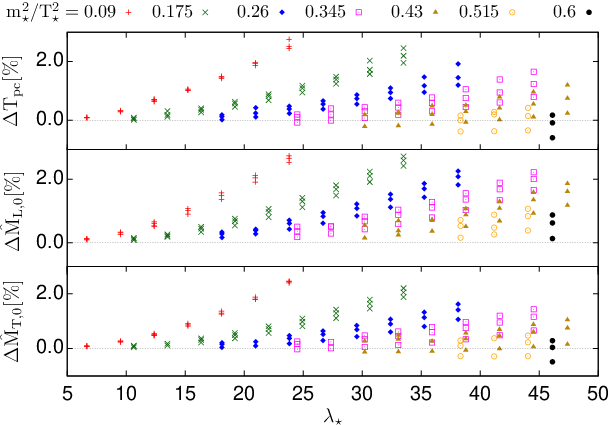
Figure 4 shows the variation of the pseudocritical temperature with the renormalization scale determined during parametrization in the physical case and in the hybrid approximation. The lines of the figure belong to different curves in the parameter space selected by different values of each of them being a line of constant physics. One sees that the dependence is less than 10%. In units of both and decrease for increasing and for large values of one can fit (up to possible logs) on and In both cases but in the chiral limit while for one has which accounts for the increase of and decrease of seen in Figure 1 and in Figure 4 for a given line of constant physics and for large We expect to diminish as we increase the order of truncation.

V.2 On the sigma mass

The parametrization reveals that there is a large region of the parameter space where a separation of scale occurs in the sense that the physical scales are much lower than the cutoff, which in turn is much smaller than the scale of the Landau pole In this case the solution of the model is practically insensitive to the cutoff used, as it was the case for in Ref. [9], where the cutoff dependence was thoroughly investigated. We have also seen that the value of the zero temperature sigma mass defined through increases with increasing . We have reached values of sigma masses which are larger than the maximal value of the sigma pole mass found within the large- approximation in Ref. [28], which in the chiral limit is MeV obtained for a coupling and a renormalization scale of MeV and MeV in the case, obtained for and MeV. The scale of the Landau pole in these cases is approximately MeV and MeV, respectively. In Ref. [29], where the renormalization scale and the value of the coupling were chosen differently, a higher value of the sigma pole mass of around 433 MeV was reported. However, in that case, the scale of the Landau pole was only 720 MeV which prevented calculations above MeV.
We investigate now what happens in our case with the scale of the Landau pole, which in view of Eq. (35) decreases with when all the other parameters are kept fixed, if a more realistic parametrization of the model is required, in which MeV to conform to recent dispersive analyses of more precise scattering data (see Ref. [27] and for a recent review Ref. [31], in particular its Figure 3). To this end, we have chosen different values of and increased the value of in the range between the and curves of the -plane, shown in Figure 1. It turns out that in the two-loop approximation it is possible to reach with the parametrization procedure described in the previous subsection values of the in the desired range. For instance, we obtain MeV and MeV for and MeV and MeV for In these cases the scale of the Landau pole remained at least seven times larger than the largest mass scale given by , that is GeV.
The interesting question is whether the scale of the Landau pole is high enough for the result not to depend too much on the value of the cutoff In order to study the sensitivity of the results on we monitored the cutoff dependence of the relative change of a given physical quantity . If this quantity is regarded as a sequence for discrete values of then in the ideal case where the convergence occurs the relative change not only tells us how sensitive is the physical quantity on the cutoff at some value but also how close it is to the convergent value. This is because if at some cutoff the value then one can say that is within % from the converged value of the physical quantity The problem is, of course, that strictly speaking the convergence would occur as but generally one cannot go above the Landau pole. Therefore, what is of practical relevance is whether the shows a plateau as a function of below the scale of the Landau pole. We investigate this in Figure 5 for several parameter sets using the quantities and at different temperatures (the relative change is shown in percentage). One can see that we are closest to a plateau if the scale of the Landau pole is high and the temperature is low. The variation of the relative change with the cutoff shows that even when the scale of the Landau pole is approximately seven times larger than for practical purposes the result can be considered compatible with a cutoff independent result, at least for temperatures not too large with respect to This result should however be interpreted with a pinch of salt since the fact that the plateau observed in Figure 5 extends up to the Landau scale is related to the fact that the physical quantities do not diverge at this scale, only the bare couplings. In higher order approximations where, due to a negatively quadratic growth of the self-energy at large frequency/momentum or to vertex-type resummations, one expects physical quantities to diverge at it is less probable that a plateau can appear if the Landau scale is too low.1616 16 Some explicit calculation using an educated example reveals that, if is large enough, a plateau develops and even extends up to the very vicinity of . However, as is decreased, the plateau fades away.
V.3 Phase transition
In the chiral limit, in both the two-loop and the hybrid approximations, the model undergoes a second order phase transition for those parameters of the plane, which are located above the line of Figure 1. This is illustrated within the two-loop approximation in Figure 6, where we show the temperature evolution of the field expectation value, curvature masses and gap masses at the lowest available momentum. The inset shows that the three numerically determined critical exponents are compatible with the values and : thus the critical behavior of the system is characterized by mean-field-type critical exponents at this level of approximation. This is expected, since they were already found to be of the mean-field type in the one-component case in Ref. [9].

One also sees in Figure 6 that fulfills the requirement of Goldstone’s theorem discussed in Sec. II.1 around Eq. (17), as it vanishes in the broken phase and becomes degenerate with in the symmetric phase. However, as a result of the truncation of the 2PI effective action, Goldstone’s theorem is violated by (approximated numerically by ) which is rather large since at small temperatures it is larger than We note however that is the smallest scale among , , and and that the size (in MeV) of the violation of Goldstone’s theorem is quite constant with the temperature. These observations give good hope that higher order corrections will reduce uniformly the violation of Goldstone’s theorem by the transverse gap mass. The restoration of Goldstone’s theorem is expected because in the absence of approximations. Our results indicate that the restoration could happen uniformly with the temperature. At large temperature both the degenerate curvature and gap masses increase, but a gap remains between them. This reflects the fact that the two-loop approximation is such that where contains all the 2PI graphs contracted with the vertices of the shifted action (see Ref. [1] for details).

In the physical case () the thermal transition is of an analytic crossover type. The temperature evolution of the order parameter is presented in Figure 7 for a set of parameters at which MeV. The solid line is obtained in the two-loop approximation, while the barely distinguishable dashed line is obtained in the hybrid approximation at the same values of the parameters. The inset shows that in the hybrid approximation is not a monotonous function of the temperature, for it shows a maximum at some value of the temperature. This reflects an inconsistency of the hybrid approximation because, as one sees in Figure 8, in the temperature range where the pressure is negative. In Figure 7, the difference between the two approximations is more visible on the longitudinal curvature mass (the transverse ones differ very little because ). The restoration of symmetry at high temperature is reflected by both the curvature and lowest momentum gap masses, as the corresponding longitudinal and transverse components approach each other. As in the chiral case, at large temperature there remains a gap between the curvature and gap masses. We note also the important difference between the values of and at . It is clearly more convenient to use the curvature masses to parametrize the model since they allow to reach higher sigma masses for the same values of the parameters.
V.4 Thermodynamics
We turn now to the study of the thermodynamic properties of the model. To this end we compute the pressure by subtracting the value of effective potential at the minimum obtained at a given temperature from the value determined at zero temperature as described below Eq. (81) of Ref. [9]. The entropy density is determined from the pressure through a numerical derivative, while the energy is calculated as Usually these quantities are divided with appropriate powers of the temperature, but we choose to normalize them to the corresponding quantity calculated for an ideal gas of massless particles. As it was the case for these three quantities when rescaled with the corresponding Stefan-Boltzmann limit agree with each other at that temperature where the interaction measure vanishes. As discussed in Ref. [9], this feature follows directly from the equations, and can be seen in Figure 8, where we compare the dependence of these quantities on the temperature in the two-loop and hybrid approximations. The curves obtained in the two cases are indistinguishable above the pseudocritical temperature. At small temperature, however, there are visible differences, and more importantly one can clearly see that the hybrid approximation is not consistent from a thermodynamic point of view, since at small temperatures it leads to negative pressure, entropy and energy densities. As already mentioned the temperature region where the pressure is negative is correlated to that where The inconsistency of the hybrid approximation is displayed also by the heat capacity which becomes negative for small temperature and by the square of the speed of sound which has a singularity at the temperature for which vanishes (see Figure 9). Note, that for the two-loop case the temperature variation of is much milder than the one shown in Figure 8 of Ref. [32] which was obtained in a Hartree approximation which included only the thermal effects and neglected the vacuum ones. This is probably related to the fact that in our case MeV is smaller than the smallest value of the corresponding mass used there.


It is visible in Figure 8 that at high temperature the pressure normalized to the Stefan-Boltzmann limit decreases with the temperature. This is the consequence of the fact that, as one can see in Figure 7, at high the masses of the excitation grow linearly with and therefore a high temperature expansion is less and less accurate with increasing
In the two-loop approximation we also tested the dependence of the pressure on the renormalization scale by choosing two points in the parameter space which belong to a line of constant physics, along which and are constant, and for which the difference in was maximal, that is around 10%. The difference in the value of corresponding to these two points was around 10% and although the difference of was around 30%, the maximal difference in the pressure was around 10% and was observed at temperatures smaller than
VI Conclusions
We studied numerically the thermal phase transition of the renormalized model, both in a genuine -derivable approximation in which the effective action is truncated at two-loop level and in a hybrid approximation in which the effective potential and the field equation derived from it are evaluated with a lower level, Hartree-Fock-type transverse (pion) and longitudinal (sigma) propagators. In the first case the self-consistent propagator equations were solved iteratively in Euclidean space using 3D cutoff regularization and the method of Ref. [9], which by a combination of adaptive numerical integration and fast Fourier transforms ensures a very accurate evaluation of the convolution-type integrals. In the hybrid approximation one obtains explicitly finite equations which are much simpler to solve.
In the chiral limit the phase transition turns out to be of second order in both approximations studied. On the one hand, this means that the higher level truncation considered in this work represents an improvement over the Hartree-Fock approximation which is known to yield a first order phase transition in the chiral limit. On the other hand, we have a clear indication that the important improvement over the Hartree-Fock level occurs in the field equation and is related to the inclusion of the setting-sun diagram. In the case of an explicit breaking of the chiral symmetry the transition is an analytic crossover.
As long as one is interested in the temperature evolution of the expectation value of the field, curvature and gap masses the hybrid approximation can be regarded as a good approximation of the two-loop -derivable approximation. In the chiral limit this is not true for the entire parameter space, as one has to restrict its application to those parameters where the longitudinal curvature mass does not change abruptly with the parameters. However, the thermodynamic study revealed its inconsistency at small temperatures for it leads to negative pressure, entropy density and energy density. In fact, this feature is also related to the nonmonotonic behavior of the field expectation value at small temperature, where it first increases with increasing temperature.
We have seen that for it is possible to achieve a realistic parametrization of the model, in which the zero temperature sigma mass, obtained as the longitudinal eigenmode of the curvature tensor, could be fixed to values around 460 MeV, while keeping the scale of the Landau pole at around 3.4 GeV. This scale is large enough for the results to be considered practically independent of the cutoff used, at least for the approximation considered here and for temperatures not too large with respect to the crossover temperature. The values of the sigma mass which can be obtained within the two-loop 2PI approximation are larger than those found in the next-to-leading order of the expansion in the 1PI formalism [28, 29], and the scale of the Landau pole proved also larger. However, in the approximations studied here, there is a significant difference between the curvature masses and the gap masses. It is expected that in approximations where the effective action is truncated at higher orders this discrepancy will diminish and then the question is raised whether this will affect the maximum value of the sigma mass achievable from the curvature mass. In this respect, it will be interesting to investigate whether the possibility of a realistic parametrization of the model persists in the 2PI formalism at higher order truncation levels and also what will be the case in the linear sigma model with three flavors at two-loop and higher truncations levels. Also, in higher order approximation, especially in those involving vertex-type resummation, as the 2PI- expansion, the presence of the Landau pole is a more severe problem, because it influences the renormalized quantities due to the divergence of the vertex function. In this case the cutoff insensitivity needs a careful reexamination and it is more probable that the scale of the Landau pole has to be kept further away from the physical scales than in the two-loop approximation discussed here.
Acknowledgements.
This work was supported by the French-Hungarian collaboration program PHC Balaton No. 27850RB (TÉT_11-2-2012). G. M. and Zs. Sz. were supported by the Hungarian Scientific Research Fund (OTKA) under Contract No. K77534 and No. K104292 and they thank A. Jakovác and A. Patkós for useful discussions.Appendix A Four-point functions
As it is discussed at length in Ref. [1] there exist three different definitions of the four-point function which do not match exactly in a given truncation. Here we shall consider these distinct definitions at in which case we can use . One possible definition is1717 17 In the approximation at hand, the kernel, and in turn the four-point function, are momentum independent, hence the absence of momenta in our notation for the kernel and the four-point function.
| (92) |
with
| (93) |
The kernel has the structure with . The four-point function admits the same decomposition and its components obey the coupled set of equations
| (94) | |||||
| (95) |
By expanding this system perturbatively, it is pretty obvious that and are not equal and thus that is not crossing symmetric. In particular, the divergent part is not crossing symmetric, which explains the need for two distinct bare couplings and . In order to solve the system of equations (94)-(95), it is convenient to consider the combinations and . It is then easily proven that
| (96) |
which shows that the combination diagonalizes the system (94)-(95). This diagonalization is in one-to-one correspondence with the one we used in the case of the Hartree gap equations in Sec. III. In fact the combinations of bare couplings and are precisely those which appeared in the diagonalized form of the Hartree-Fock gap equations. We obtain
| (97) | |||||
| (98) |
which we use in the main text to derive the expressions for and from the renormalization and consistency conditions. A second definition of the four-point function which depends on one momentum1818 18 In principle, a four-point function depends on three independent momenta. The four-point functions we consider here are taken for particular values or configurations of their external momenta and can thus depend on fewer variables. is
with
and
| (101) | |||||
| (102) |
Once again the appropriate combination of components leads to a system of decoupled equations for and which is suited in particular to extract the expressions for the bare couplings . According to Ref. [1], the third possible definition of the four-point function is given by
Using the tensor decomposition of , we check that (in other words and thus has the crossing symmetry) with
where we note that the contributions from the and components of and contribute independently to . This expression is used in the main text in order to obtain .
Appendix B Hybrid extras
In this section we give some expressions encountered in the hybrid approximation and discuss their particular aspects in some details.
B.1 Expression of
As mentioned in the main text, the four-point function is modified in the hybrid case. Following the same strategy as in the previous section, we arrive at
Once again , with
| (106) | |||||
from which we deduce Eq. (40).
B.2 Finiteness of and
Let us show that and defined in (67) and (70) are finite. One possibility is to compute the divergent part of the setting-sun sum integrals and check that and are free of divergences. As far as is concerned this was done within dimensional regularization in Appendix B of Ref. [9]. We can treat along similar lines. With the exception of the setting-sun integral all the integrals needed to obtain the finite expression of are given in Ref. [9]. Using the method of Ref. [33], one can obtain for this setting-sun integral a decomposition in terms of zero, one and two statistical factors analogous to Eq. (B5) of Ref. [9]. From that point on, the calculation of and parallels that of and performed there and uses the vacuum part of the setting-sun integral with two different masses. For the part with no statistical factors one has to expand the factors of the product to because both contain divergences. Using for the expression given in Sec. 3 of [34] one obtains
| (107) | |||||
where is the trigamma function, and the function is defined as
| (108) |
with being the Clausen function and Note that The part with one statistical factor reads
| (109) | |||||
where
| (110) | |||||
| (111) |
with Finally, the part with two statistical factors is
where
| (113) | |||||
with and all other integrals are given in Ref. [9].
We can also discuss the finiteness of and using another explicit method, which is less calculational and shows clearly the different roles played by and . Let us illustrate it in the case of . Using the results of Ref. [33] to write
| (114) |
and
| (115) | |||||
with and where denotes the analytical continuation of the bubble sum integral to real values of the frequency followed by its evaluation on shell . Plugging this back into the first line of Eq. (67), we obtain
where , and . The role of is thus to remove the subdivergences in such a way that the integrands in Eq. () are finite. In addition the last two integrals are finite due to the presence of the thermal factors. This is not the case for the zero temperature integral because the factor does not decrease fast enough in the UV. However the term involving the ratio has precisely the same form as this integral. Separating the part of and combining it with the rest we obtain
| (117) | |||||
where decreases fast enough to make the corresponding integral convergent. A similar proof can be given for
B.3 Explicitly finite field equation
We give here the explicitly finite form of the field equation. Differentiating Eq. (68) with respect to and taking into account the implicit dependence on of the gap masses one obtains
| (118) |
where, in order to give a compact expression, we have already used in the first two terms, coming from the Hartree-Fock part, the solution of the two linear equations for the derivatives of the gap masses which are obtained from Eqs. (62) and (63) as
| (119) |
with and Both and are finite because the divergence of the perturbative bubble integral does not depend on the mass. We note that for one has and therefore with the notation the field equation simplifies to
| (120) | |||||
In Eq. (118), is defined in Eq. (69) and whose explicit expression is given in Eq. (B12) of Ref. [9], is obtained from , defined in (67), upon differentiation with respect to Finally, and are obtained from given in Eq. (70) upon differentiation with respect to and respectively.
In order to determine the curve in the plane, discussed below Eq. (89), we have to take the limit and in Eq. (118). This is straightforward, except for the last term where , which at comes only from , diverges and vanishes in this limit. Working out the limit one obtains
| (121) |
As a last remark, note that there is no equivalent of the line in the case, since this requires and and by examining Eq. (120) at one sees that the two conditions cannot be satisfied simultaneously. This is because, for , is finite, but diverges as while the denominator diverges only as meaning that in this limit is the only solution of the field equation.
B.4 Solution of the gap equation at and
We show here that the solution(s) of Eq. (42) can be given at in terms of the two real branches of the Lambert function defined to be the multivalued inverse of the function , for complex. This function verifies for any complex The real branches of the Lambert function are depicted in Figure 10. The upper branch is usually called and the lower one
At one can rewrite Eq. (42) as
| (122) |
where and is defined in Eq. (83). With a few algebraic manipulations (exponentiation and multiplication by ) and using the definition of the Lambert function, one expresses the solution of Eq. (122) as
| (123) |
For (points below the line of Figure 1) the argument of is negative and one sees by looking at Figure 10 that for one has no solution if and two solutions if one smaller and one bigger than where is the accurate estimation of the Landau pole given in (IV.4) (the two solutions merge when ). The lower scale solution is given by the lower branch of the Lambert function.1919 19 We know that at one has and this can be obtained only with which diverges negatively when its argument vanishes. The use of the other branch would give a finite value, because for small The larger scale solution is given by the upper branch For one has one solution, bigger than and given by

In conclusion, to obtain the curve, defined as , we have to take the solution (123) given by the lower branch of the Lambert function and use it in Eq. (86), which can be solved only numerically. For small negative arguments can be evaluated using the asymptotic series given in Ref. [35]. We mention finally that the upper branch plays a role because we have considered the renormalized gap equation in its continuum limit. If we would consider it in the presence of a finite 3D cutoff, the solutions corresponding to the upper branch would be absent, see Ref. [15].
Appendix C Tensor decomposition
Let us first consider a real symmetric tensor such that for any rotation
| (124) |
The case is easily treated. For any we have
| (125) |
Since the fundamental representation of is irreducible, it follows from Schur’s lemma that is either or invertible. If we chose to be an eigenvalue of (there exists at least one eigenvalue since is real and symmetric), cannot be invertible and thus . For reasons that will appear below, the case requires that we distinguish from . Let us consider the case first. Since is real and symmetric, it is diagonalizable, that is it admits linearly independent eigenvectors. Let us consider an eigenvector which is not collinear to (such an eigenvector exists for ). If is a rotation that leaves invariant, we have from (124):
| (126) |
which shows that we have indeed at least linearly independent eigenvectors corresponding to the eigenvalue . If the remaining eigenvector corresponds also to , we have with that is with a function of only. If the remaining eigenvector corresponds to another eigenvalue , it has to be collinear to . If it were not, we could construct linearly independent eigenvectors, different from the previous ones and it would follow that that is , which contradicts our assumption . From this and the fact that the subspaces are orthogonal to each other, it follows that
| (127) |
with and functions of only. The case is particular because the solution to Eq. (124) is much more general than (127). In fact, because is Abelian, any tensor of the form
| (128) |
with , obeys Eq. (124). The converse can also be proven to be true. By imposing that Eq. (124) holds not only for any but also for any , one recovers the form (127).
References
- [1] J. Berges, Sz. Borsányi, U. Reinosa, J. Serreau, Annals Phys. 320, 344-398 (2005).
- [2] N. Petropoulos, J. Phys. G25, 2225 (1999).
- [3] N. Tetradis and C. Wetterich, Nucl. Phys. B 398, 659 (1993).
- [4] K. Ogure and J. Sato, Prog. Theor. Phys. 102 209 (1999).
- [5] P. B. Arnold and O. Espinosa, Phys. Rev. D 47, 3546 (1993) [Erratum-ibid. D 50, 6662 (1994)].
- [6] Y. Nemoto, K. Naito and M. Oka, Eur. Phys. J. A 9, 245 (2000).
- [7] G. Baym, Phys. Rev. 127, 1391 (1962).
- [8] J. T. Lenaghan, D. H. Rischke, J. Phys. G26, 431-450 (2000).
- [9] G. Markó, U. Reinosa and Zs. Szép, Phys. Rev. D 86 085031 (2012).
- [10] E. Seel, S. Struber, F. Giacosa and D. H. Rischke, Phys. Rev. D 86, 125010 (2012).
- [11] G. Aarts, D. Ahrensmeier, R. Baier, J. Berges and J. Serreau, Phys. Rev. D 66 045008 (2002).
- [12] U. Reinosa, Proceedings of SEWM2002, Heidelberg, Germany edited by M. G. Schmidt (River Edge, N.J., World Scientific 2003). hep-ph/0302115.
- [13] G. Fejős and Zs. Szép, Phys. Rev. D 84, 056001 (2011).
- [14] U. Reinosa and Zs. Szép, Phys. Rev. D 85 045034 (2012).
- [15] U. Reinosa and Zs. Szép, Phys. Rev. D 83 125026 (2011).
- [16] M. Bordag and V. Skalozub, J. Phys. A 34 461 (2001).
- [17] M. Bordag and V. Skalozub, Phys. Rev. D 65 085025 (2002).
- [18] A. Arrizabalaga and J. Smit, Phys. Rev. D 66 065014 (2002).
- [19] G. Amelino-Camelia, Nucl. Phys. B 476 255 (1996).
- [20] G. Amelino-Camelia, Phys. Lett. B 407 268 (1997).
- [21] G. Amelino-Camelia and S. -Y. Pi, Phys. Rev. D 47 2356 (1993).
- [22] G. Fejős, U. Reinosa, J. Serreau and Zs. Szép, work in progress.
- [23] J. -P. Blaizot, A. Ipp, A. Rebhan and U. Reinosa, Phys. Rev. D 72, 125005 (2005).
- [24] S. Borsányi and U. Reinosa, Phys. Rev. D 80, 125029 (2009).
- [25] M. Galasi et al., GSL Reference Manual (Version 1.15, 2011), http://www.gnu.org/software/gsl/manual/gsl-ref.ps.gz.
- [26] B. Fornberg, Math. of Comp. 51, 699 (1988).
- [27] J. Beringer et al. [Particle Data Group Collaboration], Phys. Rev. D 86, 010001 (2012).
- [28] A. Patkós, Zs. Szép and P. Szépfalusy, Phys. Lett. B 537, 77 (2002).
- [29] J. O. Andersen, D. Boer and H. J. Warringa, Phys. Rev. D 70, 116007 (2004).
- [30] J. Gasser and H. Leutwyler, Annals Phys. 158, 142 (1984).
- [31] J. R. Pelaez, arXiv:1301.4431 [hep-ph].
- [32] B. -C. Li and M. Huang, Phys. Rev. D 80, 034023 (2009).
- [33] J. -P. Blaizot and U. Reinosa, Nucl. Phys. A 764 393 (2006).
- [34] A. I. Davydychev and J. B. Tausk, Nucl. Phys. B 397, 123 (1993).
- [35] F. Chapeau-Blondeau and A. Monir, IEEE Trans. Signal Process. 50, 2160 (2002).