Theory of helicity-sensitive terahertz radiation detection by field effect transistors

Introduction. Field effect transistors (FETs) can be used for efficient detection of terahertz radiation [1, 2, 3, 4]. The standard model [1] assumes that the radiation is coupled to the transistor by an effective antenna which generates an ac voltage predominantly on one side of the transistor (e.g. between source and gate contacts). Since the ac gate-to-channel voltage modulates both the electric field and the electron concentration in the channel, the current density will contain a dc component, which leads to a photoresponse in the form of a dc source-drain voltage $\Delta U$ proportional to the radiation intensity. Terahertz radiation detection and imaging by FETs was demonstrated in many experimental works, see reviews in Refs. [4, 5].

For a number of applications it is essential to characterize the polarization of terahertz radiation. The strong sensitivity of FET detectors to linear polarization has been demonstrated [6, 7, 8] and was shown to be caused by the anisotropic sensitivity of the effective antennas (formed by bonding wires and contact pads). However the problem of general terahertz polarimetry, including the determination of circular or elliptical polarization is still open. The first step in this direction was made in the recent experiments of Drexler et al [9], who discovered the strong sensitivity of the FET detector to the helicity of terahertz radiation, i.e. to the sign of the phase shift between the $x$ and $y$ components of the radiation field.

The qualitative explanation of this finding is based on the assumption (which was verified experimentally) that there are two effective antennas connected to the source and the drain sides of the transistor. One of them is predominantly sensitive to the $x$-polarization and the other one – to $y$-polarization. For circularly polarized radiation, the ac voltages of these antennas are thus phase-shifted by $90^{\circ}$. To detect the helicity, the photoresponse must depend on this phase shift. This in turn is possible only because of the mixing of the ac signals produced in the channel by the two antennas.

To understand the conditions for such mixing one should take into account that (i) the condition $\omega\tau\ll 1$ is normally satisfied, where $\omega$ is the radiation frequency and $\tau$ is the momentum relaxation time and (ii) under this condition the ac current injected at the source leaks to the gate through the distributed gate-to-channel capacitance on a distance defined by the ac leakage length $l$ [3]. Thus the mixing of ac signals produced by the source and drain antennas can occur only if the gate length $L$ is comparable to the leakage length $l$. If $L\gg l$, the mixing becomes exponentially small.

This article presents a theoretical study of the helicity-sensitive detection of terahertz radiation by FETs within the two-antenna model [9] explained above. We show that to describe the required mixing of the two signals one has to abandon the usual assumption that the antennas can be considered as ac voltage sources (i. e. having zero ac impedance). Such mixing can occur only when the antennas impedances are comparable to or greater than the transistor impedance, and in particular when the antennas are current sources (infinite impedance). We calculate the FET photoresponse, including its helicity-sensitive component, as a function of the gate length $L$ and gate voltage $V_{g}$. This component has a maximum for certain values of these parameters.

The problem. We consider a FET with antennas at both the source and the drain sides, as presented in Fig. 1. The antennas are assumed to generate ac voltages $U_{a}\cos\omega t$ and $U_{b}\cos\bigl(\omega t+\theta\bigr)$ respectively, $\theta$ being the phase shift. To simplify the calculations we assume that the antennas have equal impedances at the radiation frequency $\omega$ denoted by $Z$. We also assume that a dc voltage $V_{g}$ is applied between the source and the gate, while the dc condition at the drain is open circuit. We consider the case $\omega\tau\ll 1$.

The basic equations are the continuity equation and the Ohm’s law [3]:

$$\frac{\partial\rho}{\partial t}+\frac{\partial j}{\partial x}=0,\hskip 28.45274ptj(x)=-\sigma\frac{\partial U}{\partial x},$$

(1)

where $\rho$ and $j$ are the electron charge and current densities in the channel, $\sigma=\rho\mu$ is the 2D channel conductivity, $\mu$ is the electron mobility, $U=V_{g}-V_{th}$ is the gate voltage swing, $V_{th}$ is the threshold voltage.

We assume that the spatial variation of $U$ is large compared to the gate-to-channel separation. Then the values of $\rho$ and $\sigma$ are determined only by the local value of $U$ (the gradual channel approximation). For an open channel ($U>0$), the plane capacitor formula is applicable:

$$\rho=CU.$$

(2)

Here $C$ is the gate-to-channel capacitance per unit area. This relation is not valid below threshold ($U<0$) as well as in the vicinity of the point $U=0$. To simplify the following calculations we will derive our results assuming Eq. (2) to hold and the electron mobility $\mu$ to be constant. We will then present the modifications needed to account for the general dependences $\rho(U)$ and $\sigma(U)$.

Combining Eqs. (1) and (2) we obtain the non-linear diffusion equation

$$\frac{\partial U}{\partial t}=\frac{\mu}{2}\frac{\partial^{2}U^{2}}{\partial x^{2}}.$$

(3)

We expand $U(x,t)=U_{0}+U_{1}(x,t)+U_{2}(x,t)$ up to the second order of perturbations induced by radiation, i.e. $U_{1}$ is the first order correction to $U_{0}$ and $U_{2}$ is the second order correction. In the first order Eq. (3) yields:

$$\frac{\partial U_{1}}{\partial t}=\mu U_{0}\frac{\partial^{2}U_{1}}{\partial x^{2}}.$$

(4)

The boundary conditions corresponding to Fig. 1 are:

$$\begin{array}[]{ll}U_{a}\cos\omega t-jZ=U_{1}&\mbox{at $x=0$},\\ U_{b}\cos(\omega t+\theta)+jZ=U_{1}&\mbox{at $x=L$},\end{array}$$

(5)

where $Z$ is the antenna impedance.

From now on we will use dimensionless variables, assuming that the voltages are in units of $U_{0}$, the coordinate $x$ and the gate length $L$ are in units of the leakage length $l=\sqrt{2\sigma/\omega C}=\sqrt{2\mu U_{0}/\omega}$ [3], and time $t$ is in units of $1/\omega$. In these units Eqs. (4), (5) are rewritten as:

	$\displaystyle\frac{\partial U_{1}}{\partial t}=\frac{1}{2}\frac{\partial^{2}U_{1}}{\partial x^{2}},$		(6)
	$\displaystyle\begin{array}[]{ll}U_{a}\cos t+\zeta\frac{\partial U_{1}}{\partial x}=U_{1}&\mbox{at $x=0$},\\ U_{b}\cos(t+\theta)-\zeta\frac{\partial U_{1}}{\partial x}=U_{1}&\mbox{at $x=L$},\end{array}$

where $\zeta=Z\sigma_{0}/l$ is the dimensionless antenna impedance, $\sigma_{0}$ is the channel conductivity in the absence of radiation. In fact, $\zeta$ is the ratio of $Z$ and the resistance of the rectifying part of the channel of length $l$.

To find the photoresponse voltage we need to consider the second order equation following from Eq. (3):

$$\frac{\partial U_{2}}{\partial t}=\frac{1}{2}\left(\frac{\partial^{2}U_{2}}{\partial x^{2}}+\frac{1}{2}\frac{\partial^{2}U_{1}^{2}}{\partial x^{2}}\right).$$

(10)

We average this equation over time and integrate twice over $x$ [3]. The constant that appears after the first integration is the dc current through FET which should be zero due to the dc open circuit condition on the drain side. Thus the photoresponse is given by

$$\Delta U=\langle U_{2}(L)-U_{2}(0)\rangle=\frac{1}{2}\Big[\langle U_{1}(0)^{2}\rangle-\langle U_{1}(L)^{2}\rangle\Big],$$

(11)

where the angular brackets denote time-averaging. If the impedance of antennas is negligible (i.e. $Z=0$), then $U_{1}(x=0)=U_{a}\cos\omega t$ and $U_{1}(x=L)=U_{b}\cos(\omega t+\theta)$. For this case we obtain the simple result:

$$\Delta U=\frac{1}{4}(U_{a}^{2}-U_{b}^{2}).$$

(12)

Therefore, if the antennas are ac voltage sources, their signals are not mixed, and consequently there is no sensitivity to the phase shift $\theta$.

Solution. The general solution of equation Eq. (6) is

$$U_{1}(x,t)=\frac{e^{it}}{2}\Big[Ae^{(1+i)(x-L/2)}+Be^{(1+i)(L/2-x)}\Big]+c.c.,$$

(13)

where $c.c.$ means complex conjugated. Therefore

$$\langle U_{1}(x,t)^{2}\rangle=\frac{1}{2}\Bigl|Ae^{(1+i)(x-L/2)}+Be^{(1+i)(L/2-x)}\Bigr|^{2}.$$

(14)

The boundary conditions Eq. (Theory of helicity-sensitive terahertz radiation detection by field effect transistors) give the equations for the coefficients $A$ and $B$:

	$\displaystyle\alpha A+\beta B=U_{a},$
	$\displaystyle\beta A+\alpha B=U_{b}e^{i\theta},$		(15)

with $\alpha=(1-\eta)e^{-\lambda}$ and $\beta=(1+\eta)e^{\lambda}$, $\lambda=(1+i)L/2$, $\eta=(1+i)\zeta$. Using Eq. (14) we can now present the photoresponse voltage given by Eq. (11) in the form

$$\Delta U=\frac{1}{4}\left\{\left|Ae^{-\lambda}+Be^{\lambda}\right|^{2}-\left|Ae^{\lambda}+Be^{-\lambda}\right|^{2}\right\}=\\ \mathrm{Re}\Bigl[\left(B-A\right)\left(A^{*}+B^{*}\right)\mathrm{sh}\lambda\;\mathrm{ch}\lambda^{*}\Bigr],$$

(16)

where the star denotes complex conjugation. With the help of Eq. (15) we obtain:

$$\Delta U=\mathrm{Re}\Bigl[\frac{U_{a}-U_{b}e^{i\theta}}{\beta-\alpha}\left(\frac{U_{a}+U_{b}e^{i\theta}}{\alpha+\beta}\right)^{*}\mathrm{sh}\lambda\;\mathrm{ch}\lambda^{*}\Bigr].$$

(17)

Finally, the expression for the photoresponse $\Delta U$ reads:

$$\Delta U=\frac{1}{4}F_{0}(U_{a}^{2}-U_{b}^{2})+\frac{1}{2}F_{1}U_{a}U_{b}\sin\theta,$$

(18)

where the coefficients $F_{0}$ and $F_{1}$ are determined by the dimensionless antenna impedance $\zeta$ and the dimensionless gate length $L$, entering via the parameters $\eta$ and $\lambda$:

	$\displaystyle F_{0}=\mathrm{Re}(G),\hskip 28.45274ptF_{1}=\mathrm{Im}(G),$
	$\displaystyle G=\frac{1}{(1+\eta\mathrm{\,cth}\lambda)(1+\eta\mathrm{\,th}\lambda)^{*}}.$		(19)

We note that the dependence of $\Delta U$ on $U_{a}$, $U_{b}$, and $\theta$ in Eq. (18) naturally follows from the symmetry of our problem resulting from the simplifying assumption that the impedances of source and drain antennas are equal. In this case, interchange of $U_{a}$ and $U_{b}$ together with the reversal of the phase shift $\theta$ should obviously change the sign of the photoresponse $\Delta U$.

In particular, the interference term containing $U_{a}U_{b}$, changes sign when $\theta$ is replaced by $-\theta$. We recall that source and drain antennas are assumed to predominantly respond to $x$- and $y$-polarizations respectively, meaning that the contribution of the interference term has opposite signs for right and left circular polarization. If the impedances of the antennas were different, $\sin\theta$ would be replaced by $\sin(\theta+\theta_{0})$, where $\theta_{0}$ is an additional intrinsic phase shift related to the impedance difference.

Let us consider some limiting cases.

a) Antennas are ac voltage sources, i.e. $Z=0$ and $\eta=0$. Then Eqs. (18) and (19) give $F_{0}=1$, $F_{1}=0$ and we retrieve the simple Eq. (12).

b) Antennas are ac current sources, i.e. $\zeta\gg 1$. In this case it is convenient to introduce the antennas’ ac current amplitudes $j_{a}=U_{a}/|\eta|$ and $j_{b}=U_{b}/|\eta|$. Using Eqs. (18) and (19), we obtain:

$$\Delta U=\frac{1}{4}f_{0}(j_{a}^{2}-j_{b}^{2})+\frac{1}{2}f_{1}j_{a}j_{b}\sin\theta,$$

(20)

where

$$f_{0}=\frac{\mathrm{sh}^{2}L-\sin^{2}L}{\mathrm{sh}^{2}L+\sin^{2}L},\hskip 17.07182ptf_{1}=\frac{2\mathrm{sh}L\sin L}{\mathrm{sh}^{2}L+\sin^{2}L}.$$

(21)

c) Long gate, $L\gg 1$. In this case the interference between source and drain ac signals vanishes, and we obtain the result similar to Eq. (12):

$$\Delta U=\frac{1}{4}\frac{\left(U_{a}^{2}-U_{b}^{2}\right)}{|1+\eta|^{2}},$$

which accounts for the finite antenna impedance.

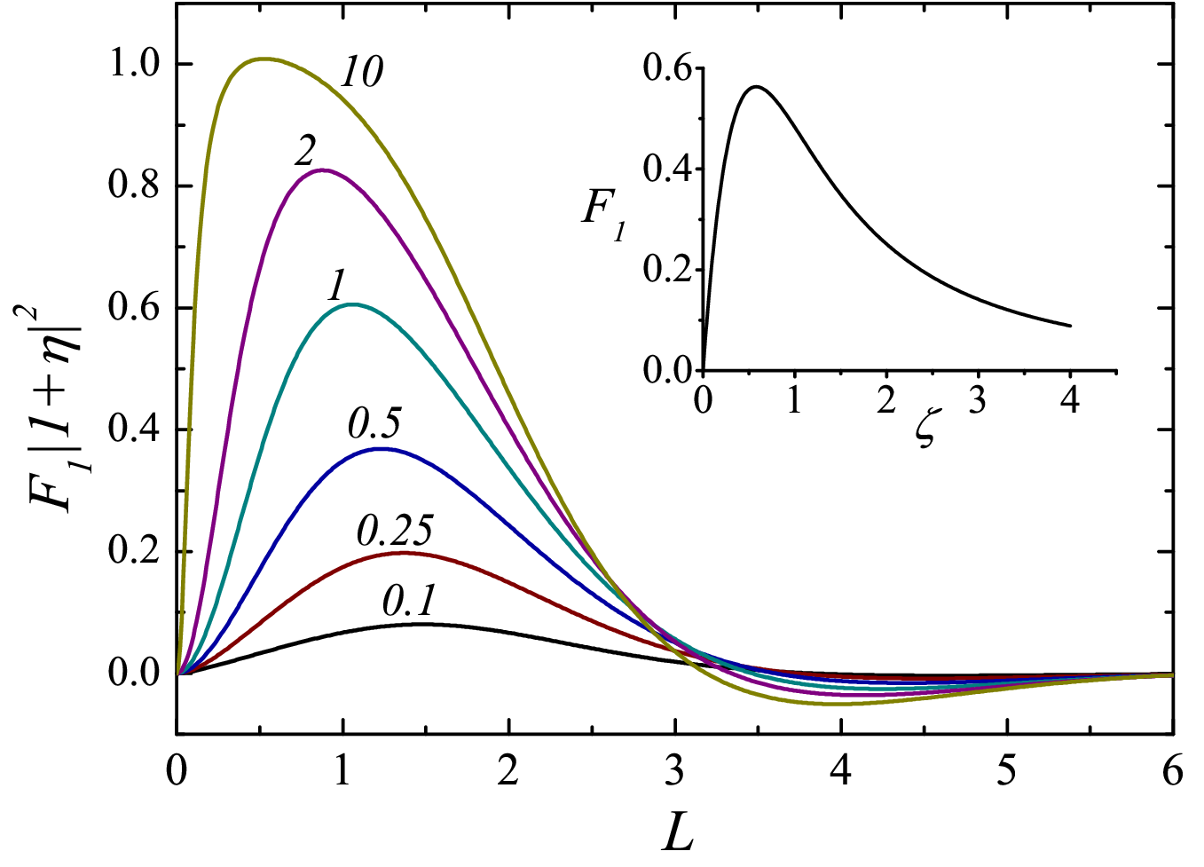
We are mostly interested in the helicity-sensitive part of the photoresponse described by the coefficient $F_{1}$ in the second term of Eq. (16). Fig. 2 presents $F_{1}$ as a function of the gate length for different values of the dimensionless antenna impedance $\zeta$. Maximum sensitivity to radiation helicity occurs when the gate length is around the leakage length $l$. As a function of $\zeta$ for a given $L$, the coefficient $F_{1}$ has a maximum around $\zeta=1$, which corresponds to ac impedance matching, see the inset in Fig. 2.

Modifications for sub-threshold regime. So far we considered detection by an open channel ($U=V_{g}-V_{th}>0$) when Eq. 2 is valid. However experimentally the maximum of the photoresponse occurs below threshold [4, 5]. Fortunately, our theory can be easily extended to arbitrary gate voltages including sub-threshold values.

Our solution of the basic Eq. 1 relied on the simple expressions $\rho=CU$ and $\sigma=\mu CU$ for the charge density and conductivity respectively, as well as on the implicit assumption that the mobility $\mu$ does not depend on $U$. This is a good approximation in the open channel regime ($U>0$). Generally, one has to consider $\rho$ and $\sigma$ as non-linear functions of $U$ not neccessarily proportional to each other. Then the derivatives $\partial\rho/\partial t$ and $\partial\sigma/\partial x$, appearing in Eq. 1, should be expessed as

$$\frac{\partial\rho}{\partial t}=\frac{\partial\rho}{\partial U}\frac{\partial U}{\partial t},\hskip 22.76228pt\frac{\partial\sigma}{\partial x}=\frac{\partial\sigma}{\partial U}\frac{\partial U}{\partial x}.$$

(22)

For the simplest situation (one ac voltage source antenna exciting a long gate FET), this consideration leads to an important generalization of the expression $\Delta U=U_{a}^{2}/4U_{0}$ [1], which reads [10, 11]:

$$\Delta U=\frac{1}{4}\Big(\frac{1}{\sigma}\frac{\partial\sigma}{\partial U}\Big)_{U=U_{0}}U_{a}^{2}.$$

(23)

This formula which replaces $1/U_{0}$ by $(\partial\ln\sigma/\partial U)_{U=U_{0}}$ is valid for arbitrary gate voltage, it also takes into account the possible dependence $\mu(U)$.

Using Eqs. 20, it can be shown that in our problem the generalisation to arbitrary dependences $\rho(U)$ and $\sigma(U)$ can be reduced to the simple change in units of length (leakage length $l$) and voltage (gate voltage swing $U_{0}$):

$$l\rightarrow\Big(\frac{\omega}{2\mu}\frac{1}{\rho}\frac{\partial\rho}{\partial U}\Big)^{-1/2}_{U=U_{0}},\hskip 11.38092ptU_{0}\rightarrow\Big(\frac{1}{\sigma}\frac{\partial\sigma}{\partial U}\Big)^{-1}_{U=U_{0}}.$$

(24)

With these modifications of units, the previous results in Eqs. (16, 17) remain valid.

Gate voltage dependence. Now we can analyze the dependence of the helicity-sensitive part of the photoresponse on the gate voltage swing $U_{0}$. This dependence is governed by the interplay of several factors: (i)change of the ac impedance of the active parts of the transitor and corresponding variation of the parameter $\zeta$, (ii)change of the ratio $L/l$ due to the variation of the leakage length $l$, and (iii)variation of the voltage unit in Eq. 22.

Assuming the mobility $\mu$ to be constant, we will use for $\rho(U)$ the semi-empirical formula [12]:

$$\rho=CU^{*}\ln[1+\exp(U/U^{*})],$$

(25)

where $U^{*}=\alpha kT/e$, $T$ is the temperature, and $\alpha$ is a phenomenological parameter on the order of 1. This formula reduces to Eq. 2 for positive $U\gg U^{*}$ and gives an exponential decrease of $\rho$ for negative $U$.

As explained above, the generalized expression for the photoresponse is given by Eq. 16 provided the voltages $U_{a}$, $U_{b}$, and $\Delta U$ are measured in voltage units in Eq. 22. However this unit is inconvenient because it itself depends on $U_{0}$. For this reason we will switch to a constant voltage unit $U^{*}$. Then Eq. 16 will have the same form, except that the coefficients $F_{0}$ and $F_{1}$, should be replaced by

$$\mathcal{F}_{0}=F_{0}U^{*}\Big(\frac{1}{\sigma}\frac{\partial\sigma}{\partial U}\Big)_{U=U_{0}},\hskip 5.69046pt\mathcal{F}_{1}=F_{1}U^{*}\Big(\frac{1}{\sigma}\frac{\partial\sigma}{\partial U}\Big)_{U=U_{0}}.$$

We have performed numerical calculations of $\mathcal{F}_{1}$ using Eq. 23. Fig. 3 shows the dependence of $\mathcal{F}_{1}$ on the dimensionless gate voltage swing $U_{0}/U^{*}$ for several values of the antenna impedance. Since the dimensionless impedance $\zeta$ changes with gate voltage, we label the curves by the values of $\zeta$ at threshold ($U_{0}=0$). Also, the gate length $L$ was taken equal to the leakage length $l$ at threshold.

One can see that the helicity-dependent contribution to the photoresponse has a maximum around or below threshold. The decrease at the left side is due to the growth of the channel resistance. As a consequence, the dimensionless antenna impedance decreases approaching the limit $\zeta=0$ with no sensitivity to helicity, see the case a) above. The decrease at the right side results from the drop of the ratio $L/l$ (see Fig. 2) caused by the increase of the leakage length $l$.

Consistent with our results, an increase of the helicity-dependent contribution to the FET photoresponse when moving towards negative gate bias was observed experimentally [9]. However, the existing experimental data is not sufficient for a detailed comparison with our results.

In summary, we have presented a theory of helicity-dependent terahertz detection by FET based on the model with two antennas connected to the source and drain sides of the transistor and sensitive to orthogonal linear polarizations. We have found the dependence of the helicity-sensitive component of the photoresponse on the antenna impedance, gate length, and gate voltage.

Acknowledgement. We thank Nina Dyakonova, Sergey Ganichev, and Maria Lifshits for interesting discussions.

References

- [1] M. Dyakonov and M. Shur, Electron Devices, IEEE Transactions on 43, 380 (1996).
- [2] M. Dyakonov and M. Shur, in Terahertz Sources and Systems, NATO Science Series, Vol. 27, edited by R. Miles, P. Harrison, and D. Lippens (Springer Netherlands, 2001) pp. 187–207.
- [3] M. Dyakonov, Comptes Rendus Physique 11, 413 (2010).
- [4] W. Knap, M. Dyakonov, D. Coquillat, F. Teppe, N. Dyakonova, J. Lusakowski, K. Karpierz, M. Sakowicz, G. Valusis, D. Seliuta, I. Kasalynas, A. Fatimy, Y. Meziani, and T. Otsuji, Journal of Infrared, Millimeter, and Terahertz Waves 30, 1319 (2009).
- [5] W. Knap and M. I. Dyakonov, in Handbook of terahertz technology for imaging, sensing and communications, Woodhead Publishing Series in Electronic and Optical Materials, edited by D. Saeedkia (Woodhead Publishing, Cambridge, 2013) p. 121.
- [6] M. Sakowicz, J. Łusakowski, K. Karpierz, M. Grynberg, W. Knap, and W. Gwarek, Journal of Applied Physics 104, 024519 (2008).
- [7] W. Knap, F. Teppe, N. Dyakonova, D. Coquillat, and J. Lusakowski, Journal of Physics: Condensed Matter 20, 384205 (2008).
- [8] S. Kim, J. D. Zimmerman, P. Focardi, A. C. Gossard, D. H. Wu, and M. S. Sherwin, Applied Physics Letters 92, 253508 (2008).
- [9] C. Drexler, N. Dyakonova, P. Olbrich, J. Karch, M. Schafberger, K. Karpierz, Y. Mityagin, M. B. Lifshits, F. Teppe, O. Klimenko, Y. M. Meziani, W. Knap, and S. D. Ganichev, Journal of Applied Physics 111, 124504 (2012).
- [10] M. B. Lifshits, in Book of Abstracts, 31st International Conference on the Physics of Semiconductors, Zurich, Switzerland, 29 July–3 August 2012, (2012) p. 242.
- [11] M. Sakowicz, M. B. Lifshits, O. A. Klimenko, F. Schuster, D. Coquillat, F. Teppe, and W. Knap, Journal of Applied Physics 110, 054512 (2011).
- [12] M. S. Shur, Introduction to Electronic Devices (Wiley, New York, 1996).