Theory of giant magnetoresistance at misfit interfaces

Interfaces between different materials are the sources of rich physics and functions. Novel phenomena emerge that are not expected from each of the constituents [1]. One example is a two dimensional metallic state appearing at the interface between two insulators LaAlO₃ and SrTiO₃ [2]. Even superconductivity appears in this two-dimensional system, which is an issue of recent intensive interests [1]. Another example is the tunneling magnetoresistance (TMR) [3]. The resistance across the interface between the two ferromagnets depends strongly on the relative direction of the magnetizations. Therefore, transport properties perpendicular to the interface offer many useful functions for applications.

An essential nature of interfaces between different systems is the misfit of the lattice constants, which often causes the distortion of the lattice structure to relax this misfit when it is not so large. In this case, the lattice constants slowly change from the interface to the bulk region, and correspondingly electrons adiabatically follow this gradual change. When the misfit is larger, on the other hand, the system can not remedy this misfit and an incommensurate situation occurs at the interface.

Incommensurate systems attract recent attention from the viewpoints of charge/spin density waves [4], localization of wavefunctions [5], and quasi-crystals [6]. In these systems, incommensurability occurs in the bulk states, which is rather exceptional or special cases. On the other hand, the incommensurability occurs very often at interfaces since there is no definite relation between the lattice constants of the two systems.

In this paper, we study theoretically the tunneling conductance across the interface between the two two-dimensional systems $A$ and $B$ with lattice constants $a$ and $b$, respectively. The ratio $a/b$ matters significantly in this tunneling process, and also its sensitivity to an external magnetic field.

Let us start with the two one-dimensional chains $A$ and $B$. The extension to two-dimensions is straightforward. We assume two chains have the same length $L$. The number of sites in chain $A$ and in chain $B$ are $N_{A}$ and $N_{B}$, which are determined from $L=aN_{A}=bN_{B}$. We assume that two chains are parallel to $x$-direction with the separation $c$, and the tunneling amplitude between the $n$th site in chain A and the $m$th site in chain B is given by

Here $d$ characterizes the spatial extent of the tunneling process. Two chains are placed in a magnetic field, which is perpendicular to the plane including two chains. The magnetic field induces AB phase (Aharanov-Bohm phase). We choose the gauge as $\bm{A}=(0,Bx)$.

We rewrite Eq. (1) by wavenumber representation as

where the wavenumbers are specified by the integers $k$ and $p$. The lattice constant $\lambda$ of the composite system of $A$ and $B$ is given by $\lambda=an_{A}=bn_{B}$, where we define as $n_{A}=\frac{N_{A}}{G_{AB}}$ and $n_{B}=\frac{N_{B}}{G_{AB}}$. $G_{AB}$ is the greatest common divisor of $N_{A}$ and $N_{B}$, and is the number of the unit cells with the lattice constant $\lambda$, i.e., $L=G_{AB}\lambda$. The translational symmetry by $\lambda\bm{e}_{x}$ leads to the conservation of wave numbers by ${\rm mod}~\frac{2\pi}{\lambda}$. The Brillouin zones are decomposed into $n_{A}$ and $n_{B}$ parts by $\frac{2\pi}{\lambda}$.

The summations in Eq. (2) can be carried out (See in the appendix) and $t_{kp}$ is obtained as

$\delta_{G_{AB}}$ is defined as

Equation (5) represents the wavenumber conservation. $\xi$ is the characteristic length of this system, which is represented as $\xi=\frac{L}{L_{AB}}=\frac{b}{n_{A}}=\frac{a}{n_{B}}$. $x_{A}$ and $x_{B}$ are solutions of the Diophantine equation $n_{B}x_{A}-n_{A}x_{B}=1.$ This equation has an integer solution because $n_{A}$ and $n_{B}$ are coprime. $(x_{A}+mn_{A},x_{B}+mn_{B})$ is also the solution, where $m$ is an arbitrary integer, but this indefiniteness is not concerned with Eq. (3) because of Eq. (5). Equation (4) represents the interference in the periodic part.

We consider the resistance at an interface between the two-dimensional systems $A$ and $B$, which are the straightforward generalization of the above chain system. The conductance $g$ per one enlarged unit cell is represented as

We take a limit $G_{AB}\rightarrow\infty$, and

with

$\bm{b}$ is the dimensionless magnetic flux penetrating the enlarged unit cell, i.e., $\bm{B}c\lambda=2\pi\bm{b}$. The resistance $R$ per the unit area is given by $R=\frac{\lambda^{2}}{g}$, which is the physical quantity of our main interest.

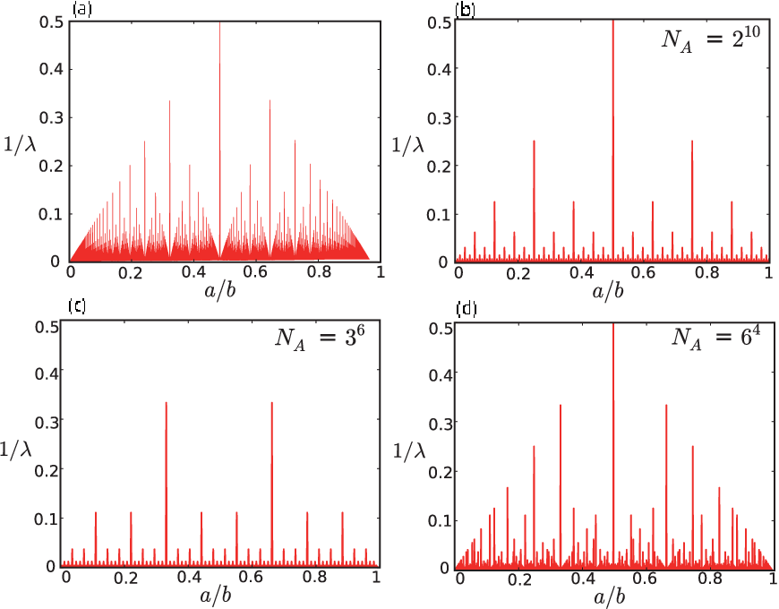
First, we study the lattice constant $\lambda$ of the enlarged unit cell. $\frac{1}{\lambda}$ change radically as the ratio $\frac{a}{b}=\frac{n_{B}}{n_{A}}=\frac{N_{B}}{N_{A}}$. Particularly, $\frac{1}{\lambda}$ indicates a fractal architecture with fixed $N_{A}$, if $N_{A}$ is a power of a prime number. We show this relation in Fig. 2 with the fixed lattice constant $a$ of chain $A$. The upper left panel indicates the global behavior of $\frac{1}{\lambda}$ v.s. $\frac{a}{b}=\frac{N_{B}}{N_{A}}$, and the rest panels show the graphs for selected $\frac{N_{B}}{N_{A}}$ with fixed $N_{A}=2^{10},3^{8},6^{4}$. When $N_{A}=2^{10},3^{8}$, it shows clear fractal structures, while it shows a complex structure when $N_{A}=6^{4}$. When $N_{A}=p^{n}$ where $p$ is a prime number, $\frac{1}{\lambda}$ is given by the following calculations. We define $S_{i}=\left\{p^{n-i},2p^{n-i},\cdots\left(p^{i}-1\right)p^{n-i}\right\}\enskip(i=1,2,\cdots n)$ and $P_{i}=S_{i}-S_{i-1}\enskip(i=1,2,\cdots n)$, where we set $S_{0}=\phi$ (empty set). The relation between $\lambda$ and $\frac{N_{B}}{N_{A}}$ is specified as

when $N_{B}\in P_{i}$. This relation and the definition of $P_{i}$ generate the fractal structure scaled by $\frac{1}{p}$. When $N_{A}$ is not a power of a prime number, this fractal structure is not there, but $\frac{1}{\lambda}$ shows a highly singular behavior as a function of $\frac{a}{b}$ as shown in panels (a) and (d) of Fig. 2.

Next, we consider the magnetic field dependence of $R$ to see the proper scaling for $\bm{B}$. In a limiting case $d\rightarrow 0$, the hopping amplitude is finite only between sites whose $x$-coordinates and $y$-coordinates are the same. In this limit, $F=1$ and it is clear that the resistivity has the period $\Delta b_{i}=1$, which is independent of $(n_{A},n_{B})$. From $\bm{B}c\lambda=2\pi\bm{b}$, the resistivity of the misfit interface is enhanced for larger $\lambda$ (or $n_{A},n_{B}$), i.e., (nearly) incommensurate case. In this case, $\xi=\frac{a}{n_{B}}$ is small, so we cannot assume $\xi\gg d$. Then there is a crossover from $d\to 0\ll\xi$ to $d\gg\xi$, and the interference in the periodic part $F$ occurs in the latter case where the period of the conductivity becomes $\Delta b_{i}=2l_{AB}$, where $l_{AB}$ is the least common multiple of $n_{A}$ and $n_{B}$. However, as will be seen for explicit examples, the variation of $R$ occurs within the scale of $\Delta b_{i}=1$ even for $d\gg\xi$.

We estimate the behavior of $R$ with $\lambda$ in the limiting cases. In a limiting case $d\rightarrow 0$, one enlarged unit cell has one pair of sites connected by the finite hopping amplitude, and hence $R$ grow as $\propto\lambda^{2}$. When $d\cong a\cong b$, which is more relevant to the realistic systems, there are many finite hopping amplitudes between sites in one enlarged unit cell, and the number of site in each chain does not becomes important. The hopping amplitude per area does not change with $\lambda$ and the scale of $R$ is nearly constant although the magnetic field dependence is sensitive to $\lambda$. In the extreme case $a\ll b$, on the other hand, the situation is similar to the case of $d=0$, and $R$ is expected to grow with $\propto\lambda^{2}$.

Now, let us study a concrete example. We assume the simplest tight binding model on a square lattice both for $A$ and $B$ as $\epsilon_{A(B)}\left(\bm{k}\right)=\cos k_{x}+\cos k_{y}$ with the chemical potential at $\mu=0$, and the magnetic field is along the $x$-axis, i.e., $b_{y}=0$. From Eq. (6) and Eq. (7), we can obtain the analytic form of the conductivity as given in the appendix. In the following calculations, we fix the lattice constant of $A$ as $a=1$ and set $\frac{t_{AB}^{2}}{2\pi^{2}}=1$.

In this model, the Fermi surfaces is straight line as indicated in Fig. 3. At the misfit interface, the Brillouin zone is reduced to $n_{A}\times n_{A}$ ($n_{B}\times n_{B}$) parts by $\frac{2\pi}{\lambda}$. The segmented pieces of the Fermi surfaces are determined by the parity of $n_{A}$ ($n_{B}$). This even-odd effect is a special properties of the linear Fermi surfaces. In Fig. 3, we indicate two examples, i.e., cases of $n_{A}=2$ and $3$.

We now consider the resistance $R$ as a function of the magnetic field $B_{x}$ and the dimensionless magnetic flux $b_{x}$. The resistance $R$ at $B_{x}=b_{x}=0$ reflect the even-odd effect of the Fermi surfaces. When both $n_{A}$ and $n_{B}$ are odd, $R=0$ for integer values of $b_{x}$. On the other hand, when either $n_{A}$ or $n_{B}$ is even, $R=0$ at $b_{x}={\rm integer}+\frac{1}{2}$. Strictly speaking, $R=0$ means the diverging $g$ and hence the perturbation theory with respect to $t_{AB}$ does not work there. This divergence has two origins, i.e., the Van Hove singularity and the fact that the forms of the Fermi surface of $\epsilon_{A}$ and $\epsilon_{B}$ are the same.

At first, we consider a limiting case $d\rightarrow 0$. The behavior of the resistance $R$ depends on the parity of $n_{A}$ and $n_{B}$, which reflects the even-odd effect of the Fermi surfaces. The maximum value of $R$ changes radically in each $n_{A}$ and $n_{B}$, which will be discussed later. $R$ has the period from $b_{x}=0$ to $b_{x}=1$, and indicates a similar behavior to $b_{x}$ for all $(n_{A},n_{B})$ except for the even-odd effect. When either $n_{A}$ or $n_{B}$ is even, the $b_{x}$ is shifted by $\frac{1}{2}$. $b_{x}$ is the dimensionless magnetic flux penetrating the enlarged unit cell, which is scaled in an appropriate manner in each case as $B_{x}c\lambda=2\pi b_{x}$. The larger $\lambda$ becomes, $R$ oscillates more rapidly as $B_{x}$. The panels (a1) and (b1) of Fig. 4 show $R$ as a function of $b_{x}$, while (a2) and (b2) shows $R$ as a function of $\frac{B_{x}ac}{2\pi}$. Panels (a1) and (a2) are for $(n_{A},n_{B})=(2,1)$, while (b1) and (b2) are for $(n_{A},n_{B})=(50,49)$. If $\lambda$ become bigger, the resistivity $R$ oscillate as $\frac{B_{x}ac}{2\pi}$ more rapidly.

Next, we consider a finite $d=a$. The behavior of the resistance $R$ is not determined only by the parity of $n_{A}$ and $n_{B}$, but it is different in each $n_{A}$ and $n_{B}$ because of the interference term $F$. The periodicity of $R$ changes from $\Delta b_{x}=1$ to $\Delta b_{x}=2l_{AB}$, but the $b_{x}$-value at which $R=0$ remains unchanged from the case of $d=0$. The panels (a1) and (b1) of Fig. 5 show $R$ as a function of $b_{x}$, while (a2) and (b2) as a function of $\frac{B_{x}ac}{2\pi}$. Panels (a1) and (a2) are for $(n_{A},n_{B})=(2,1)$, while (b1) and (b2) are for $(n_{A},n_{B})=(50,49)$. In the similar way to the case of $d=0$, the larger $\lambda$ become, the $R$ oscillates as $b_{x}$ changes of the order of 1 and hence more rapidly as a function of $\frac{B_{x}ac}{2\pi}$.

Establishing the enhanced magnetoresistance by $\lambda$, we next discuss the maximum value of the resistance $R_{\rm max}$ in the region $0\leq B_{x}ac\leq 2\pi$. $R_{\rm max}$ indicates a singular behavior as a function of $\frac{a}{b}=\frac{N_{B}}{N_{A}}$ in (a1) and (a2) of Fig. 6 for two cases $d=0$ and $d=a$, respectively. Both show the rather complex and singular behavior, but these are neatly organized as a function of $\lambda$ as shown in (b1) and (b2) of Fig. 6. When $d\to 0$ (((b1)), $R_{\rm max}$ increases as $\lambda$ as expected for all the regions of $a/b$ (asymptotically $\lambda^{2}$ in the large $\lambda$ limit). For $d=a$ (((b2)), on the other hand, $R_{\rm max}$ stays almost constant and independent of $\lambda$ for $a\cong b$, while it approaches to the behavior of $d=0$ as $a/b$ decreases.

Now we discuss about the relevance of the present results to real systems. The disorder effect at the interface gives the mean free path $\ell$. When the size $\lambda$ of the enlarged unit cell is larger than $\ell$, the singular dependence on $a/b$ is broadened. In other words, the enhancement of the magnetoresistance saturates by the factor $\sim$min$(\ell,\lambda)^{2}$. The most relevant case to the real systems is that $a\cong b$ and $d\cong a$. In this case, the scale of the resistance $R$ per unit area does not sensitively depends on the ratio $a/b$, while the magnetoresistance is determined by $\lambda$ and depends strongly on the ratio $a/b$ in a singular way. The essence of the enhanced magnetoresistance is the sensitive change in the interference pattern of the wavefunctions within the enlarged unit cell induced by the magnetic flux, it is expected that the magnetic field perpendicular to the interface also gives the similar effect to the parallel case discussed in the present paper.

In summary, we have studied the magentoresistance at the interface with misfit of lattice constants. We found that resistance R depends on the ratio a/b of the two lattice constants in a singular way, and the size $\lambda$ of the enlarged unit cell determines the magnitude of the magnetoresistnce, which can he enhanced orders of magnitudes when $a/b$ is a (nearly) irrational number.

The authors acknowledge the fruitful discussion with Y. Kawaguchi, K. Burch, M.Kawasaki and Y.Tokura. This work is supported by Grant-in-Aid for Scientific Research (Grants No. 24224009) from the Ministry of Education, Culture, Sports, Science and Technology of Japan, Strategic International Cooperative Program (Joint Research Type) from Japan Science and Technology Agency, and Funding Program for World-Leading Innovative RD on Science and Technology (FIRST Program).

References

• [1] H.Y. Hwang et al., Nat. Mat. 11(2), 103 (2012).
• [2] A. Ohtomo, and H. Y. Hwang, Nature 427(6973), 423 (2004).
• [3] J.S. Moodera et al., Phys. Rev. Lett. 74, 3273 (1995).
• [4] P. Bak, Rep. Prog. Phys. 45, 587 (1982).
• [5] J.B. Sokoloff, Phys. Rep. 126, 189 (1985).
• [6] E.L. Albuquerque, and M.G. Cottam, Phys. Rep. 376, 225 (2003).