Reduced Density Matrix after a Quantum Quench
Abstract
We consider the reduced density matrix (RDM) for a finite subsystem after a global quantum quench in the infinite transverse-field Ising chain. It has been recently shown that the infinite time limit of is described by the RDM of a generalized Gibbs ensemble. Here we present some details on how to construct this ensemble in terms of local integrals of motion, and show its equivalence to the expression in terms of mode occupation numbers widely used in the literature. We then address the question, how approaches as a function of time. To that end we introduce a distance on the space of density matrices and show that it approaches zero as a universal power-law in time. As the RDM completely determines all local observables within , this provides information on the relaxation of correlation functions of local operators. We then address the issue, of how well a truncated generalized Gibbs ensemble with a finite number of local higher conservation laws describes a given subsystem at late times. We find that taking into account only local conservation laws with a range at most comparable to the subsystem size provides a good description. However, excluding even a single one of the most local conservation laws in general completely spoils this agreement.
I Introduction
Recent advances in systems of optically trapped ultra-cold atomic gases have made it possible to observe the nonequilibrium time evolution of isolated many particle systems over long time scales [1, 2, 3, 4, 5, 6]. A key property of such cold atomic clouds is their weak coupling to the environment and resulting smallness of external dissipative processes. To a good approximation one is dealing with isolated quantum mechanical many particle systems, which are prepared in generally mixed states, and one is interested in the time dependence of observables, in particular at late times. The experimental results have stimulated theoretical efforts aimed at understanding the principles underlying the nonequilibrium dynamics of isolated many particle systems. Some of the most basic questions are whether observables generally relax to time-independent values, and if they do, whether their stationary values are described by a statistical ensemble. Other prominent issues concern the roles of dimensionality and conservations laws. Experiments on trapped atoms[2] established that three-dimensional condensates rapidly relax to a stationary state characterized by an effective temperature, whereas constraining the motion of atoms to one dimension leads to a much slower relaxation to a non-thermal distribution. It was argued that this observed difference has its origin in the presence of additional (approximate) conservation laws, related to quantum integrability, in the one dimensional case. Theoretical efforts aimed at understanding these and related questions [7, 8, 9, 10, 11, 12, 13, 14, 15, 16, 17, 18, 19, 20, 21, 22, 23, 24, 25, 26, 27, 28, 29, 30, 31, 32, 33, 34, 35, 36, 37, 38, 39, 40, 41, 42, 43, 44, 45] indicate that in translationally invariant models there are at least two basic types of behaviours at late times: subsystems either thermalize [46], i.e. are characterized by a Gibbs distribution with an effective temperature, or they are described by a generalized Gibbs ensemble (GGE) [8]. There is evidence that the latter applies to integrable models, while the former constitutes the “generic” situation.
A popular protocol for analyzing nonequilibrium evolution is a so-called quantum quench: here the system is originally prepared in the ground state of some local, short ranged Hamiltonian , where is a system parameter such as a magnetic field or an interaction strength. At time , is then suddenly “quenched” to , and the subsequent time evolution under the new Hamiltonian is studied. Under this protocol the system remains in a pure state at all times, and as a whole can clearly never be described by a Gibbs or generalized Gibbs distribution. This can be seen by considering the hermitian operators
| (1) |
where and are eigenstates of with energies and respectively. Then the expectation values
| (2) |
are oscillating in time and never become stationary. A useful and intuitive point of view is to focus on local properties of a given system in the thermodynamic limit, i.e. ask questions only about observables contained in a finite subsystem [13, 31, 32]. Here the (infinitely large) complement of can act as an effective bath, and probability may freely dissipate from to . As a result may be described by a mixed state. Arguably the most precise and convenient description of this situation is in terms of the reduced density matrix of subsystem . The latter is obtained from the density matrix of the entire system as
| (3) |
A central question is then, whether for any finite subsystem
| (4) |
where is a time-independent reduced density matrix obtained as
| (5) |
If (4) holds, then the system evolves towards a stationary state described by the distribution . In particular (4) implies that the expectation values of any local operator acting only within subsystem is given by
| (6) |
An efficient way of investigating whether a given RDM approaches a known stationary distribution at late times was introduced in Ref. [20] by considering the operator norm . If this approaches zero at late times, then the system relaxes locally to the stationary distribution . Ref. [20] was concerned with the case where describes a thermal ensemble with a given effective temperature, and considered very small subsystems. Here we are interested in a quench to a quantum integrable model. As we have alluded to before, the stationary state for such quenches is believed to be described locally by a generalized Gibbs ensemble (for the model we consider below this was established in Ref. [32]). More precisely, the density matrix of the entire system is expected to be of the form
| (7) |
where is a normalization11 1 We have in mind regularizing the system by enclosing it in a very large but finite volume., and are local conserved quantities, i.e. local operators such that
| (8) |
The Lagrange mutipliers are fixed by the requirements
| (9) |
We stress that the GGEs considered in the quench context are fundamentally different from thermal ensembles, because through the specific values of the Lagrange multipliers they retain an infinite amount of information about the initial state. Above we have stipulated that only local (in space) conservation laws are to be included in the definition of , but it is in fact a matter on ongoing debate whether locality is a necessary or even desirable requirement [47]. In this context a result obtained in Ref. [31] is rather illuminating: there it was demonstrated for a particular example, the transverse field Ising chain, that different statistical ensembles can have identical local properties. The two ensembles considered were a GGE of the form (7), and the so-called “pair ensemble” obtained by time averaging the quench density matrix . Given that is generally not unique, it is clearly desirable to identify the simplest description. To that end we introduce truncated generalized Gibbs ensembles of the form
| (10) |
and investigate how well such ensembles describe the stationary state for quenches to integrable models.
The outline of this paper is as follows. In section II we review some relevant results for the transverse field Ising chain. Local conservation laws are presented in section III and used in sections IV, V, VI to define several classes of generalized Gibbs ensembles. Properties of corresponding reduced density matrices are discussed in section VII. In section VIII we discuss general properties of distances on the space of reduced density matrices and introduce the distance used in the remainder of the paper. In sections IX, X, XI and XII we present results for the distance between quench and generalized Gibbs reduced density matrices. We summarize our results in section XIII. Various technical issues are discussed in four appendices.
II Some Facts about the Transverse-Field Ising Chain (TFIC)
Here we briefly review some relevant results on the TFIC. The latter is an important paradigm for quantum phase transitions in equilibrium [48] as well as non-equilibrium dynamics[49, 14, 29, 24, 31, 32, 36]. In the latter context experimental realizations range from cold atomic gases [50] to circuit QED [51]. The Hamiltonian of the model on a ring is
| (11) |
where . The quantum spins can be mapped to (real) Majorana fermions by means of the Jordan-Wigner transformation
| (12) |
where . In terms of the Majorana fermions (12), the Hamiltonian takes a block-diagonal form
| (13) | |||||
Here is the number operator
| (14) |
and by construction commutes with . The two blocks and correspond to periodic and antiperiodic boundary conditions on the fermions respectively. They can be diagonalized by Bogoliubov transformations
| (15) |
where the Bogoliubov angle is given by
| (16) |
The diagonal form of the Hamiltonian is
| (17) |
where the single-particle energy is given by
| (18) |
The ground states of are the fermionic vacua
| (19) |
Here the momenta are , where are even/odd integers for R and NS fermions respectively.
II.1 Quantum Quenches
Our quench protocol is as follows: we prepare the system in the ground state for an initial value of the transverse magnetic field. At time we instantaneously change the field from to . The state of the system at times is obtained by evolving with respect to the new Hamiltonian
| (20) |
An important quantity is the difference of Bogolibov angles required to diagonalize and respectively
| (21) |
As we are interested in obtaining results in the thermodynamic limit we have to distinguish between two cases.
II.1.1 Quenches from the Paramagnetic Phase
Here the initial state in a large, finite volume is simply the NS vacuum
| (22) |
The time evolved state can then be written in the form [31]
| (23) |
where is the ground state of and a normalization factor.
II.1.2 Quenches from the Ferromagnetic Phase
Here our initial state in a large, finite volume must reflect the spontaneous symmetry breaking of the spin-flip symmetry in the thermodynamic limit. The appropriate choice is [31]
| (24) |
III Local Conservation Laws in the TFIC
We consider the one dimensional transverse field Ising chain in the thermodynamic limit
| (25) |
Following Ref. [52] we can construct an infinite number of local conservation laws
| (26) |
where the Hamiltonian itself is . Let us define operators
| (27) |
and
| (28) |
In terms of these operators the local conservation laws are
| (29) |
They are local in the sense that the density of involves only spins on neighbouring sites. By virtue of their locality, the conservation laws can all be expressed in terms of Jordan-Wigner fermions (12)
| (30) |
We now realize that all conservation laws (30) are in fact quadratic in Majorana fermions! It is then a simple matter to diagonalize them simultaneously by means of a Bogoliubov transformation (15), where on the infinite chain the Bogoliubov fermion operators have anticommutation relations
| (31) |
The conservation laws take the simple form
| (32) | ||||
which furthermore shows that they are even/odd under spatial reflections. Interestingly the conservation laws do not depend on the transverse field and are therefore shared by the entire one-parameter family of Hamiltonians . This seems to be a generic feature of models with a free fermion spectrum like the TFIC, see App. C and Ref. [58].
III.1 Local conservation laws for periodic boundary conditions
Above we focussed on the bulk contribution to the local conservation laws. For a finite system on a ring there are boundary contributions, which can be determined as follows. In terms of the Bogoliubov fermions, the conservation laws for periodic boundary conditions are
| (33) | |||||
| (34) |
where the momenta are taken to be either in the R or NS sectors. By inverting the Bogoliubov transformation and Fourier transforming back to position space, one obtains a representation of the conservation laws in terms of the Majorana fermions for periodic/antiperiodic boundary conditions respectively. Finally, inverting the Jordan-Wigner transformation gives the desired expression in terms of spins.
IV Generalized Gibbs Ensemble
We now define the density matrix of a generalized Gibbs ensemble formally by the expression
| (35) |
where is a normalization that ensures . In practice we need to regularize (35) in an asymptotically large, finite volume .
The Lagrange multipliers are fixed through the requirements
| (36) |
Using translational invariance we can alternatively work with the densities of the conservation laws
| (37) |
to rewrite (36) as
| (38) |
The solution to this system of equations is
| (39) |
where and is defined in (21). In Fig. 1 we show for a quench from to .
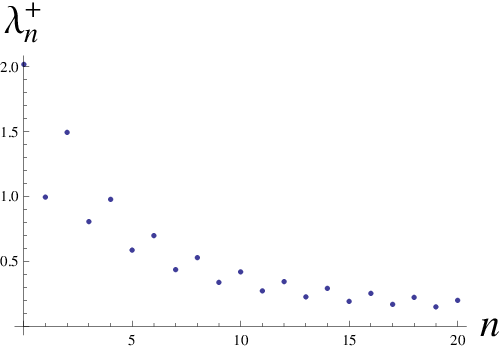
The large behaviour of Eq. (39) is determined by the regions (where the integrand has a logarithmic singularity) and one can show that
| (40) |
where the sign is for quenches within the same phase and otherwise. We see that the Lagrange multipliers decay rather slowly as a function of .
IV.1 GGE in terms of mode occupation numbers
In the literature the generalized Gibbs ensemble is often constructed from mode occupation numbers , see e.g. [8, 12, 18, 53, 54]. The latter are non-local (in space) as they involve a Fourier transform. We will now establish the relation between this and our definition (35). It follows from (32) that the density matrix can be rewritten in the form
| (41) |
where
| (42) |
This establishes the fact that the GGE density matrix can be constructed either from the local conservation laws (30), or from the mode occupation numbers . This relationship generalizes to interacting integrable models, where the appropriate GGE can be formulated either in terms of the local integrals of motion generated from the transfer matrix, or from the mode occupation numbers , where are Faddeev-Zamolodchikov operators [55, 56].
V Truncated Generalized Gibbs Ensembles
In order to assess the importance of the various conserved quantities, it is useful to define ensembles that interpolate between the Gibbs distribution and the GGE. We define particular such truncated GGEs as follows. Given that the densities of the conservation laws involve neighbouring sites, it is natural to retain only the “most local” conservation laws, i.e.
| (43) |
Here is an integer and () corresponds to the Gibbs ensemble (GGE). The Lagrange multipliers are obtained from the requirements
| (44) |
where . Eqns (44) are a consequence of and the assumption that the stationary state after the quench is described by RDMs based on (43). For transverse field quenches we have , but the other Lagrange multipliers are different from their respective values in the full GGE, i.e.
| (45) |
We note that the correlation matrix of can be computed efficiently using FFT algorithms. This is in contrast to the case of theories with non-trivial scattering matrices, for which it is extremely difficult to reconstruct the Lagrange multipliers from the conservation laws [57].
VI Defective Generalized Gibbs Ensembles
It is instructive to consider a second type of truncated GGE, where we retain an infinite, but incomplete set of integrals of motion. Such “defective” GGEs will allow us to ascertain the role of a particular local conservation law. We define the truncated defective GGE as the density matrix ()
| (46) |
in which the Lagrange multipliers are fixed by the system (36) with , , and we have used that the Lagrange multipliers must vanish as a consequence of reflection symmetry around the origin. We then define the defective GGE as the limit of truncated defective GGEs:
| (47) |
In order to solve the system of equations (36) for the defective GGE it is useful to work in the mode occupation number representation (41), which reads
| (48) |
where the Lagrange multipliers are subject to the set of equations
| (49) |
Guided by the fact that and form an orthonormal set of functions on , we look for a solution of the form
| (50) |
where is a yet to be determined constant. We note that the value of affects the expectation values of local operators. For some cases can be easily determined as follows. Given that , (50) implies that
| (51) |
Setting then gives
| (52) | ||||
Eqs (52) allow us to identify cases, in which :
- 1.
odd and quenches within the same phase;
- 2.
even and quenches across the critical point.
Importantly, implies that , i.e. the defective GGE is identical to the full GGE. This “GGE reconstruction” is a peculiarity of free-fermion models and can be traced back to the existence of conservation laws independent of the quench parameter, see also Ref. [58].
For general quenches and values of , is determined by Eq. (47). We find that it takes the value corresponding to the maximal entanglement entropy (as shown in Fig. 9), although the entanglement entropy may be non-stationary under a variation of the excluded integral of motion (see Appendix D for further details).
VII Reduced Density Matrices in the Transverse Field Ising Chain
In this section we summarize some basic features of RDMs in the TFIC. We note that most of the following discussion generalizes straightforwardly to other spin chains with free fermionic spectra such as the quantum XY model. Our starting point is a density matrix describing the entire system, which we take to be of size with periodic boundary conditions. We are interested in the limit , but it is convenient to start with a large, finite chain. The RDM of a subsystem consisting of spins at sites , can be expressed in the form
| (53) |
where and . The quantum spins are mapped to (real) Majorana fermions by the Jordan-Wigner transformation (12). The nonlocality of the transformation (12) has important consequences for RDMs. First and foremost, if the spins are not adjacent, the map from spin to fermionic degrees of freedom does not have a simple reduction to the subspace of the Hilbert space formed by sites , because of Jordan-Wigner strings stretching between sites [59, 60]. However, the RDM of a block of adjacent spins can be mapped one-to-one on a block of adjacent fermions [61, 62], provided that the first site of the block coincides with site , i.e. the origin of Jordan-Wigner strings. Then (53) can be represented in the form
| (54) |
with . An important quantity in what follows is the correlation matrix
| (55) |
In the cases of interest to us, the correlation matrix is of block-Toeplitz form
| (56) |
where
| (57) |
The TFIC Hamiltonian exhibits a symmetry
| (58) |
If the density is invariant under the transformation (58) we have , and as Wick’s theorem applies to the Jordan-Wigner fermions we can express (54) as a Gaussian [62]
| (59) |
where ensures that and is a skewsymmetric, -by- Hermitian matrix related to by
| (60) |
We now turn to the three particular cases of interest, namely those where in (53) is a thermal density matrix, a GGE density matrix, or the density matrix after a global quantum quench of the transverse field in the TFIC.
VII.1 Thermal Density Matrix
On a very large ring, the Hamiltonian has a block diagonal structure, see section II. The thermal density matrix is a function of the Hamiltonian and therefore inherits the same block structure
| (61) |
It follows from this that only even operators have non-vanishing expectation values, i.e.
| (62) |
In the thermodynamic limit the difference between expectation values of local operators with respect to the R and NS sectors tends to zero, so that we may work exclusively in e.g. the R sector. The resulting RDM of a contiguous block of spins is then Gaussian (59), (60) with
| (63) |
It can be written in the form (56) with
| (64) |
VII.2 GGE Density Matrix
It was shown in Ref. [32] (see also [24, 31]) that the RDM of the generalized Gibbs ensemble (35),(41) is Gaussian and can be expressed in the form (59), (60). The correlation matrix is given by
| (65) |
It can be written in the form (56) with
| (66) |
Here the ’s are related to the ’s by (42) and the Bogoliubov angle is given in (16).
VII.3 Truncated GGE Density Matrix
VII.4 Defective GGE Density Matrix
In Sec. VI we defined the defective GGE as the ensemble that lacks in the conservation law . Its correlation matrix is given by
| (69) |
It can be written in the form (56) with and (cf. Eq. (66))
| (70) |
where is computed numerically maximizing the entanglement entropy, which selects whenever it is allowed. We note that the Fourier transform of Eq. (70), which is required to compute the correlation matrix (57), can be easily expressed in terms of the GGE correlators; for we have
| (71) |
Since is a bounded function of (cf. Eq. (52)), at fixed the fermionic correlators approach the GGE ones at least exponentially fast in .
VII.5 Quench Density Matrix
At zero temperature the ground state phase diagram of the TFIC exhibits ferromagnetic () and paramagnetic () phases, separated by a quantum critical point. In the ferromagnetic phase the symmetry of the Hamiltonian is broken spontaneously. As we will see, this symmetry breaking has important effects on the time evolution of the density matrix.
VII.5.1 Quenches originating in the paramagnetic phase
Here at the full quench density matrix is
| (72) |
where the state is given in (23). As a result of the squeezed-state form of , Wick’s theorem applies to averages calculated with respect to , and RDMs are Gaussians of the form (59), (60), with correlation matrix
| (73) |
This is of the form (56) with
| (74) |
where is given by (16).
VII.5.2 Quenches originating in the ferromagnetic phase
Given the initial state (24), the post-quench density matrix of the full system is
| (75) |
Importantly, RDMs are no longer Gaussian in this case. We will discuss how to cope with this complication in section XI. It is known [32] that in the stationary state RDMs are Gaussian with a correlation matrix equal to the limit of (73).
VIII Distances on the Space of RDMs
In the following we focus on RDMs for finite subsystems of lattice models with a finite dimensional Hilbert space at each site. In this case the RDMs are finite dimensional matrices and a simple way to define a distance between two density matrices is by means of a matrix norm
| (76) |
Here the index labels different matrix norms. As we are dealing with finite matrices, all norms are equivalent in the sense that
| (77) |
where and are positive numbers that depend on the matrix dimension but are independent of . One consequence of (77) is that if the distance between two matrices approaches zero when some external parameter is tuned to a value , the dependence of the distance on is almost independent of the norm. On the other hand, the dependence on matrix dimension is in general very different for different norms. This is important for our purposes, because the matrix dimension is related to the size of the subsystem under consideration, and it is principally desirable to be able to compare distances between different sizes.
From a technical point of view, the distance induced by the Frobenius norm22 2 It is also known as the “Hilbert-Schmidt norm”, but we prefer to call it “Frobenius norm” to emphasize that we are considering finite subsystems.
| (78) |
is generally the easiest to calculate. On the other hand, it has the drawback that the physical interpretation of the distance is less transparent than for some other norms. For instance, given two density matrices and , a very natural question is how different expectation values of local observables are in the two ensembles. We now discuss this question for the particular case of spin-1/2 quantum spin chains. Here the most important local observables are products of Pauli matrices. These are particular cases of involutions , for which the following inequality holds
| (79) |
Here
| (80) |
is the trace norm. From Eq. (79) it is evident that the trace distance provides an upper bound for the difference between the expectation values of observables in the two states: if , then the expectation values of all (local) observables will agree in the two ensembles within accuracy . In terms of the Frobenius distance we have instead (here we use that the local Hilbert space is two-dimensional)
| (81) |
On the other hand, we have
| (82) |
where in the last step we have used that for involutions
| (83) |
Combining (82) and (81) we see that as long as , the Frobenius distance does not provide useful information about expectation values. It is shown in Appendix A that for sufficiently large this is always the case.
A second problem with using the Frobenius norm as a distance is that the norms of RDMs at late times after a quantum quench, as well as the norms of RDMs describing Gibbs or generalized Gibbs ensembles, generally are exponentially small in the subsystem size. Given the upper bound derived in Appendix A
| (84) |
this implies that in these cases of interest is exponentially small in subsystem size. This shows that the Frobenius norm itself is not a convenient measure for the distance between two density matrices. The same problem occurs for the operator norm , where is the largest eigenvalue of . This norm was used for example in Ref. [20] to analyze the relaxation properties of small subsystems after a quench into a nonintegrable model. Indeed we have
| (85) |
and the maximal eigenvalues of RDMs for large subsystems are generally exponentially small in subsystem size.
VIII.1 Definition of the Distance
In order to circumvent the problem described above, we define our ‘‘distance’’33 3 We have not proven that obeys the triangle inequality as this is not essential for our purposes. on the space of RDMs as
| (86) |
1. An upper bound: Using the upper bound derived in (171) we see that
| (87) |
2. A lower bound: A lower bound for can be established by means of the triangle inequality . Using that the Frobenius norm of a RDM is related to the second Rényi entropy by
| (88) |
we find that
| (89) |
This provides the desired lower bound
| (90) |
We note that the bound (90) is independent of subsystem size as long as the second Rényi entropies of the two ensembles differ at least by a constant (when viewed as functions of ).
VIII.2 The Distance between two Thermal Ensembles
In order to establish a benchmark for (86), it is useful to consider the distance between the RDMs of two thermal ensembles at slightly different inverse temperatures and (but the same Hamiltonian). Then
| (91) |
For a sufficiently large subsystem (and a local Hamiltonian), the first factor on the right hand side can be expressed as
| (92) | |||||
where . For a large subsystem, this is proportional to the square of its size, and hence
| (93) |
We conclude that the distance between two thermal RDMs on a subsystem of size , and is
| (94) |
As expected this is proportional to the difference in temperatures, but there is also a factor of . The latter is important if one is interested in comparing the distance between two ensembles for different subsystem sizes.
VIII.3 The Distance between two GGEs
The above discussion carries over to the case of two generailzed Gibbs ensembles (35), with slightly different values of Lagrange multipliers . The leading contribution to the distance is given by
| (95) |
A calculation similar to the thermal case shows that for large subsystem size
| (96) |
VIII.4 Information on observables contained in the distance
Let us consider the situation where the distance between two reduced density matrices and defined on an interval of length becomes small, and denote the corresponding averages of local operators on said interval by
| (97) |
By expanding the density matrices in a complete basis of Hermitian involutions we can show that
| (98) |
Defining an average
| (99) |
we can express the distance (86) as
| (100) |
Here
| (101) |
is the relative difference between the ensembles described by and , respectively. This implies that measures the mean relative difference of the expectation values of all local operators, averaged with respect to the probability distribution (99).
VIII.5 The Distance between two Gaussian Density Matrices
The distance (86) between two Gaussian RDMs and can be expressed in terms of their correlation matrices following Ref. [59]. Given the definition of the distance
| (102) |
we require tractable expressions for the quantities
| (103) |
This is achieved in two steps. First, we note that the product of two Gaussian RDMs (59) is itself Gaussian[59]
| (104) |
This can be seen by expanding the left hand side of (104) by means of the Baker-Campbell-Hausdorff formula in terms of multiple commutators, and then observing that the commutator of quadratic operators is quadratic and gives rise to a commutator between the matrices that characterize the 2-forms
| (105) |
Second, using results for the second Rényi entropy [63], one can relate the Frobenius norm of a Gaussian RDM to the correlation matrix by
| (106) |
Combining (106) and (104) one can then show [59] that
| (107) |
Here we have used that , which is a consequence of density matrices being positive semidefinite operators. Finally, substituting (107) into (102), we obtain the following result for the distance between two Gaussian RDMs
| (108) |
Given that the correlation matrices are only dimensional (with the subsystem size), (108) provides a very efficient way of computing distances for large subsystem sizes.
IX Single-site subsystem
It is instructive to consider the time evolution of the RDM describing a single-site subsystem in some detail. In this case the RDM of site can be expressed in the form
| (109) |
where is the magnetization per site at time after the quench, i.e.
| (110) |
The RDM of the generalized Gibbs ensemble describing the stationary state is
| (111) |
where
| (112) |
Finally, the RDM of the thermal ensemble described by , whose inverse temperature is fixed by the requirement
| (113) |
is given by
| (114) |
Here the transverse magnetization per site is
| (115) |
IX.1 Quenches originating in the paramagnetic phase
Here the symmetry enforces
| (116) |
The z-component of the magnetization per site is
| (117) |
For late times we may evaluate the integral by means of a stationary phase approximation, which gives
| (118) |
where
| (119) | |||||
The distance between and the generalized Gibbs RDM at late times then decays to zero like a power-law with exponent
| (120) | |||||
On the other hand, the distance between and the thermal RDM approaches a constant at late times
| (121) |
IX.2 Quenches originating in the ferromagnetic phase
Here all three components of the magnetization per site are non-zero. The component along the transverse field direction is again given by (117), while the late-time asymptotics of has been calculated in [31]
| (122) |
Here is a known amplitude and . Finally, the Heisenberg equation of motion for relates the and components
| (123) |
Importantly, exhibit exponential decay in time. In contrast, again decays like a power law with exponent and therefore will dominate the late time behaviour. Hence at sufficiently late times, the distances of to GGE and thermal RDMs are again given by (121) and (120) respectively. So for a single site subsystem the spontaneous symmetry breaking only modifies the intermediate time behaviour of the distances. As we will see, this holds true also for larger subsystems.
X Larger Subsystems for Quenches from the Paramagnetic Phase
For quenches with and in the thermodynamic limit, we determine the distance between the quench RDM and that of an appropriate thermal or generalized Gibbs ensemble by means of relation (108). The correlation matrices for all cases are of the form (56), (57) with elements given in (64), (66) and (74) respectively. For a subsystem of size this requires the calculation of determinants of matrices, which is done numerically. Results for a quench from to and subsystem sizes are shown in Figs 2 and 3

We see that the distance between quench and Gibbs RDMs tends to a -dependent constant at late times. This establishes that subsystems do not thermalize. On the other hand, as can be seen from Fig. 3, at sufficiently late times the distance between and decays to zero in a universal power-law fashion
| (124) |


The large- asymptotics of the function can be inferred as follows. On surfaces with constant, small the time scales as as is shown in Fig. 5. This in turn implies that
| (125) |

X.1 Relaxation time
We may extract a relaxation time from the behaviour of the distance, by using the connection to averaged differences in the expectation values of local operators established in subsection VIII.4. The distance can be written as
| (126) |
where
| (127) |
and the bar denotes the average (99). Using that
| (128) |
and then substituting the asymptotic behaviour (124), (125) into the right hand side, we obtain
| (129) |
Bounding the right hand side by a (small) constant, we obtain a time scale associated with the relaxation of the average relative error with respect to the distribution (99)
| (130) |
It is not simple to identify the observables that give significant contribution to the average, since it depends both on their “multiplicity” in the subsystem (produced by translational invariance and other symmetries) and on the expectation values. We note that the relaxation time is very different from the time scales identified in Ref. [32] in the time evolution of the two point functions of spin operators for quenches within the paramagnetic phase.
X.2 Distance from Truncated Generalized Gibbs Ensembles
Having established that the distance between quench and GGE reduced density matrices tends to zero as a universal power law at late times, a natural question is, how close the quench RDM is to the truncated GGEs (43), which retain only finite numbers of conservation laws.

A representative example for a quench within the paramagnetic phase is shown in Fig. 6. We see that at sufficiently late times, the distances converge to constant values. However, increasing the range (and number) of conservation laws, the values of these plateaux decrease, signalling that retaining more conservation laws gives better descriptions. In an intermediate time window, the extent of which grows with , the distance decays in a universal power-law fashion. In Fig. 7 we consider the distance
| (131) |
between the RDMs of the truncated and full generalized Gibbs ensembles as a function of the parameter . For a given subsystem size , this corresponds to plotting the values of the plateaux seen in Fig. 6 against the corresponding values of . The distance is seen to start decaying exponentially as a function of as soon as .

There are two main conclusions of the above analysis:
- 1.
Including more local conservation laws improves the description of the stationary state.
- 2.
The description of the stationary state improves rapidly, once the range of all conservation laws not included in the truncated GGE exceeds the subsystem size .
X.3 Distance from defective Generalized Gibbs Ensembles
We now turn to the role played by particular local conservation laws. We find that the distance between quench and defective GGE reduced density matrices for a given quench and subsystem size tends to a constant at late times, i.e.
| (132) |
The dependence of this asymptotic value on the subsystem size and the integer is shown in Fig. 8 for a quench within the paramagnetic phase.

We see that exhibits an exponential decay in as soon as . This is similar to the behaviour observed in the truncated GGE case. The decay length can be calculated from the large- asymptotics of Eq. (71). By series expanding Eq. (108) to second order in we obtain
| (133) |
Numerically we find that .
X.3.1 “GGE Reconstruction”
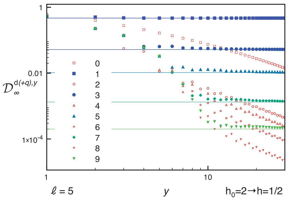
In section VI we discussed the issue that, for certain quenches and omitted conservation laws , the corresponding defective GGE is identical to the full generalized Gibbs ensemble. We now return to this point. In Fig. 9 we consider the truncated, defective GGE for a quench across the critical point from to for a subsystem of length . We plot the distance between the reduced density matrices of the appropriate GGE and the truncated, defective GGE with integrals of motion, where () has been excluded, i.e.
| (134) |
As discussed in section VI, for even we expect this distance to approach zero, when the number of conservation laws goes to infinity. This behaviour is clearly observed in Fig. 9. This implies that the corresponding conservation laws do not affect averages of local operators. As discussed before, this is a particular feature of free theories, where and generically share certain local conservation laws.
X.3.2 More local conservation laws are more important
On the other hand, for odd we find that approaches constant values when becomes large. This value agrees with the distance between the GGE and the defective GGE with maximal entanglement entropy (we stress that for the considered quench the defective GGE does not always correspond to a stationary point of the entanglement entropy under a variation of the excluded integral of motion, as shown in Fig. 20 of Appendix D).
The fact that tends to a constant at large shows that retaining an infinite number of local conservation laws while excluding one of them is insufficient for describing the stationary state. By comparing distances for different values of we observe that for a given value of , decreases as a function of . This implies the more local the conservation law, the more important it is for describing the stationary state.
XI Quenches from the ferromagnetic phase: effects of spontaneous symmetry breaking.
We now turn to quenches originating in the ferromagnetic phase, i.e. . In this case, the time evolved initial state is given by
| (135) |
where are the ground states of the Hamiltonian with periodic/antiperiodic boundary conditions. In order to analyze reduced density matrices after a quantum quench from the ferromagnetic phase we will make use of the following facts.
- a)
The fermion parity Eq. (14) is fully factorized in space.
- b)
The states and are eigenstates of with eigenvalues and respectively.
- c)
The difference between the expectation values of local operators in the states and tends to zero in the thermodynamic limit.
- d)
The RDMs , , where is a single interval and its complement, are Gaussian.
Property b) allows us to express the full density matrix in the form (cf. Eq. (53))
| (136) | |||||
where ensures that and is a complete set of Hermitian involutions with the property
| (137) |
We will refer to as even and odd operators respectively. The main difference between even and odd operators, is that the latter are not local in terms of fermions: a Jordan-Wigner string is attached to them. We are interested in the RDM of a block of contiguous spins, which is obtained by tracing out the degrees of freedom outside
| (138) |
A convenient representation for is obtained by restricting the sums in Eq. (136) to involutions that act as the identity operator outside the interval , i.e.
| (139) |
where the superscript indicates that the operators act on the Hilbert space over all sites in . As a result of property a), fermion parity has a simple restriction onto the interval
| (140) |
and can be used to subdivide operators into even and odd ones
| (141) |
This then implies that we can decompose the RDMs of (136) into even and odd parts as well
| (142) |
In the thermodynamic limit we then may employ property c) to obtain the following expressions
| (143) |
Importantly, the even part is Gaussian (59) by virtue of property d), and has the same structure as RDMs for quenches originating in the paramagnetic phase. On the other hand, the odd part has its origin in the spontaneous breaking of the symmetry. The commutation relations (141) imply that for any Gaussian density matrix , because the latter is by construction even. As a result the odd part of the RDM enters the distance from a Gaussian state only through its norm
| (144) |
We will be interested in the cases where describe Gibbs or (truncated) generalized Gibbs ensembles. The Frobenius norms , and can be efficiently evaluated by means of Eq. (108). What remains in order to determine the distance (144) is a method for calcuating the Frobenius norm . This is a somewhat involved technical problem, which is addressed in Sec. XI.1 and Appendix B. The basic idea is to utilize a cluster decomposition theorem at any finite time after the quench, see also Ref. [36].
XI.1 from cluster decomposition
The main difficulty in calculating the Frobenius norm of is that the latter is not Gaussian. The idea is therefore to obtain as a reduction of a Gaussian operator. To that end, we consider a composite system consisting of our subsystem and a single site at position , which is separated from by a block of length , see Fig. 10.

The even part of the RDM can be expanded in a complete basis of Hermitian involutions as
| (145) | |||||
where , since both and in (145) are even operators with respect to fermion parity. In the limit of large separation , we may use the cluster decomposition principle to simplify the expectation values
| (146) |
This then leads to the following relation between RDMs in the limit or large separation
| (147) |
where is the RDM of site . The piece of interest to us is
| (148) |
In the next step we move from spins to Majorana fermions by means of the Jordan-Wigner transformation (12)
| (149) |
where are odd products of Majorana fermions acting on sites within . Importantly, the fermionic expression (149) depends on the configuration of Majoranas in subsystem through the Jordan-Wigner string operator. The right hand side of (149) can be cast in the form
| (150) |
where is a normalized, Gaussian operator (59) acting on the Hilbert space over sites
| (151) |
In writing (149) we are assuming . The fact that is Gaussian is a consequence of the particular form of (which is the analog of (23) in the R sector) and being quadratic in fermions. The odd part of the single-site RDM is of the form
| (152) |
and hence
| (153) |
Here the late-time behaviour of are given by (122) and (123) respectively, and following Ref. [31] they can be easily calculated numerically for all times. Combining (153) and (150) we obtain
Since both p and are Gaussian, their moments can be written in terms of their respective correlation matrices
| (155) |
We note that the correlation matrices are related by , with the diagonal matrix that changes the sign of the last 2-by-2 block ( is the identity)
| (156) |
Using (107) we have
| (157) |
A slight complication arises because p is not positive semidefinite. To account for this we must use the more general definition of as the product of the eigenvalues of with halved degeneracy [59]. We may then recast (XI.1) in the form
| (158) |
While formally correct, (158) is not suitable for numerical computations, because at large distances becomes very close to zero. A more convenient expression derived in Appendix B is
| (159) |
Here is the correlation matrix of the interval and is given by (56), (57), (74). In order to utilize (159) we in principle have to consider infinite separations and hence infinitely large matrices.
Crucially, in practice a finite separation , where is the maximal propagation velocity, is sufficient to recover the limit up to corrections that are exponentially small in . Here is the correlation length in the initial state. A representative example is shown in Fig. 11.

In practice, using a finite with provides an efficient way for calculating and then by means of (144) distances for quenches originating in the ferromagnetic phase.
XI.2 Results for quenches from the ferromagnetic phase
For quenches with and in the thermodynamic limit, we determine the distance between the quench RDM and that of an appropriate thermal or generalized Gibbs ensemble by means of relations (144) and (159). The correlation matrices for all cases are of the form (56), (57) with elements given in (64), (66) and (74) respectively. For a subsystem of size most terms require the calculation of determinants of matrices, which is easily done numerically. The evaluation of is significantly more costly, and in practice involves determinants of at most matrices, as discussed above.

We see that the distance between quench and Gibbs RDMs tends to a -dependent constant at late times. On the other hand, as shown in Fig. 13, at sufficiently late times the distance between and decays to zero in a universal power-law fashion
| (160) |

The large- asymptotics of the function can be inferred in the same way as for quenches within the paramagnetic phase. On surfaces with constant, small , time scales as as is shown in Fig. 14, which implies that
| (161) |

We conclude that the late time behaviour of the distance between quench and generalized Gibbs RDMs is the same as for quenches within the paramagnetic phase. The mean relaxation time is therefore again given by (130). Interestingly this coincides with the result obtained in Ref. [32] for the relaxation of the order parameter two-point function after quenches within the ferromagnetic phase. The effects of the spontaneous symmetry breaking are important only at short and intermediate times. It is shown in the inset of Fig. 13 that there is a time window, in which the odd part of the RDM gives the dominant contribution to the distance, which decays exponentially.
XI.3 Magnitude of the contribution due to
The effects of the spontaneously broken symmetry in the initial state make themselves felt through the -odd part of the density matrix. The relative importance of for large can be estimated by considering the von Neumann entropy of subsystem
| (162) |
We recall that the von Neumann entropy after a global quench grows linearly in time until the Fermi time , and then saturates to a value proportional to the subsystem size [65, 64]. Using the commutation relations (142) we see that the even part can be expressed in terms of the full RDM as follows
| (163) |
Since for any set of density matrices the von Neumann entropy satisfies[66] (, )
| (164) |
the following bounds on the von Neumann entropy of subsystem hold
| (165) |
This demonstrates that at any time after the quench the symmetry breaking contribution to the von Neumann entropy will be at most . Given that for large subsystems the von Neumann entropy at late times is proportional to , we conclude that the relative contribution of the odd part of the RDM will be important only for small subsystem sizes.
XI.3.1 A conjecture for in the limit of large and
We now consider the space-time scaling limit[31]
| (166) |
We observe that in this limit our numerical results for quenches within the ferromagnetic phase are in excellent agreement with the following relation
| (167) |
Here we have highlighted the asymptotic nature of the relation and indicated by , where the most important corrections will arise. Since is proportional to the Rényi entropy (cf. Eq. (88)), we may use the known results [64] on the asymptotics of the latter
| (168) |
Combining (168) and (167) provides a conjecture for the asymptotic behaviour of . This conjecture is compared to numerical results in Fig. 15. The agreement is clearly quite good.

XII Quenches across the critical point
We now turn to quenches across the critical point. These are of particular interest [14, 31, 42]. In Fig. 16 we plot the distance between quench and GGE reduced density matrices for a quench from the ferromagnetic phase () to the paramagnetic phase (). The 15 data sets displayed correspond to subsystem sizes between and . We find that the distance again decays in a universal power law.

In Fig. 16 we consider the same quench, but focus on very small subsystem sizes . We observe that the distance displays an oscillatory behaviour on top of a power-law decay in time. This is in agreement with the analytic results discussed in section IX.2 for the case. Increasing the subsystem size leads to a rapid suppression of the amplitude of the oscillations.

In Figs 18 and 19 we consider the reverse quenches, i.e. starting at in the paramagnetic phase, and quenching to in the ferromagnetic phase. The behaviour of the distances is very similar to what we found for the quench from to : at late times the distance decays as a power law, and for small subsystem sizes we observe oscillatory behaviour on top of this decay.


XIII Summary and Conclusions
In this work we have considered the evolution of reduced density matrices after a quantum quench in the transverse field Ising chain. The main result of our work is to demonstrate that
| (169) |
where is the reduced density matrix of a subsystem consisting of adjacent spins after a quench of the transverse field, and is the reduced density matrix of an appropriately defined generalized Gibbs ensemble. The derivation of (169) is based on defining an appropriate distance on the space of reduced density matrices, and then establishing that the distance between quench and GGE reduced density matrices approaches zero at late times. For our particular choice of distance we found that at late times this distance approaches zero as a universal power law in time
| (170) |
We have presented a detailed construction of in terms of the local (in space) integrals of motion of the TFIC. The densities of these conservation laws involve only spins on consecutive sites. We proved that these local conservation laws are related in a linear fashion to the occupation numbers of the Bogoliubov fermions that diagonalize the Hamiltonian of the TFIC. This linear relation establishes the equivalence of our construction of the GGE to the one frequenctly used in the literature, which is based on mode occupation numbers.
We then have addressed the question, which of the conservation laws are most important for obtaining an accurate description of the stationary limit of the quench RDM. To that end we introduced (defective) truncated generalized Gibbs ensembes, which are missing some of the local conservation laws. We found that the more local the conservation laws (i.e. the fewer consecutive spins their densities involve), the more important they are for describing the stationary state of a given subsystem. Loosely speaking we observed that in order to obtain a good description of the stationary state RDM of a subsystem of size , we need to retain all local conservation laws, whose densities involve at most neighbouring spins, where is a constant depending on and . Leaving out “highly local” conservation laws generally provides a very poor description of the stationary state. To the best of our knowledge this is the first such demonstration of a connection between locality of conservation laws and their importance in the GGE context.
Our work raises a number of issues. First and foremost is the dependence of the results obtained on the precise definition of the distance on the space of reduced density matrices. We have argued, that the “best” distance is the one based on the trace norm, because it provides the most direct and precise information on the time evolution of local observables. Unfortunately this distance is much harder to handle analytically. It would however be very interesting to implement it in purely numerical studies using iTEBD or related algorithms.
Acknowledgements.
We thank P. Calabrese and J. Eisert for helpful discussions. This work was supported by the EPSRC under grants EP/I032487/1 and EP/J014885/1 and the National Science Foundation under grant NSF PHY11-25915 (FHLE). FHLE is grateful to the KITP in Santa Barbara for hospitality.Appendix A Inequalities involving the Frobenius norm of RDMs for spin-1/2 Quantum Spin Chains
In this appendix we provide lower and upper bounds for the Frobenius norm of the difference of two reduced density matrices in a translationally invariant system. An upper bound is obtained as follows
| (171) | |||||
Here we have used that both and are positive semidefinite and hence
| (172) | |||||
where are the eigenvalues of . To derive a lower bound we start by expressing the RDM of a block of spins in a spin- chain in the form
| (173) |
where with , and is the density matrix of the full system; is only function of the length because of translational invariance. By singling out the term with , we can express this in the form
| (174) |
where is the RDM of the block consisting of sites . We also write the RDM of the spin
| (175) |
and observe that
| (176) |
Here we have defined . Using (174) we have
| (177) | |||||
where we have used that for matrices we have in the second step, and (176) in the last. Iterating Eq. (177) times we obtain
| (178) |
This implies that for sufficiently large subsystem size , the distance will generally be larger than .
Appendix B Derivation of Eq. (159)
Our starting point is Eq. (158), i.e.
| (179) |
Our task is to evaluate
| (180) |
where and is the diagonal involution defined in (156). We recall that denotes the product of the eigenvalues of with halved degeneracy (the eigenvalues of are always double degenerate [67] for antisymmetric matrices and ). The correlation matrix defined in Eq. (155) turns out to be [59] the Schur complement of the block matrix of the matrix , i.e.
| (181) |
Here denotes the matrix, whose rows and columns are associated with spatial regions and respectively, e.g.
| (182) |
Here is the size of subsystem , while is the distance between and site , see Fig. 10.
The first step is to find determinant representations for and , where is a generic symmetric involution ( and ).
We first consider . Since is antisymmetric, its eigenvalues come in pairs
| (183) |
Both eigenvalues give rise to the same eigenvalue of , and hence
| (184) |
Here the product is over all positive eigenvalues of . Using that
| (185) |
it follows that
| (186) |
Next we consider . The matrix
| (187) |
satisfies and . Since we have
| (188) |
the eigenvalues of and coincide. Therefore
| (189) |
where in the last step we used Eq. (186). Since and , (189) can be rewritten in the form
| (190) |
Using (186) and (190), we can reexpress the quantities in (180) as follows:
| (191) | ||||
Here we have use that the expectation value of the string operator in region is related to the correlation matrix by . A remaining problem is that , which precludes a numerical evaluation of (179) on the basis of expressions (191). This complication is overcome as follows. We recall the expression of the determinant of a block matrix
| (192) |
We then substitute (181) into (191), and identify and as the determinants of the matrices
| (193) |
respectively. Rearranging some of the rows and columns we obtain
| (194) | ||||
The representations (194) are suitable for numerical calculations even in the limit of large . There is one further simplification: in the limit we have
| (195) |
To see this, we expand the determinants in (194) with respect to the last -by- block (from here on we omit the subscript in , i.e. )
| (196) |
Using properties of the correlation matrix one could show that the determinants on the second line approach zero in the limit of large distance. For the sake of simplicity we propose a different proof, which is based on the assumption that the limit
| (197) |
exists: we demonstrate that the limit cannot be infinite, so the expression in Eq. (196) does tend to zero as . To this end we consider the correlation matrix of a generic Gaussian density matrix, and show that the determinant has an upper bound independent of . Hence it cannot diverge in the limit . Our proof is based on the following facts:
- (a.)
, and hence and ;
- (b.)
cannot have more than eigenvalues with absolute values exceeding .
Property (a.) is a consequence of being the correlation matrix of a positive semidefinite Gaussian. Property (b.) can be proved as follows: Let a normalized vector with for any . Then
| (198) |
where the inequality follows from property (a.). If there were more than eigenvalues of with modulus larger than , we could find a linear combination of the corresponding normalized eigenvectors with the property for any ; this leads to a contradiction with (198) since
| (199) |
This completes the proof of property (b.).
Properties (a.) and (b.) imply that
| (200) |
which establishes that the determinants in (196) remain finite in the limit . Concomitantly the expression in Eq. (196) approaches zero as . This establishes (195). Putting everything together we see that (194) can be written as
| (201) |
which is Eq. (159).
Appendix C Conservation laws in spin models with free fermion spectra
In this appendix we present a simple construction of the bulk contribution to local conservation laws of the TFIC on the infinite line. Our method readily generalizes to other models with free fermionic spectrum such as the XY chain. Ignoring boundary conditions, we can use the Jordan-Wigner transformation to express the Hamiltonian as a quadratic form in Majorana fermions
| (205) |
Here is a skewsymmetric block-circulant matrix
| (206) |
where are 2-by-2 matrices. In Fourier space we have
| (207) |
where . One can show that a complete set of local conservation laws is obtained by taking
| (208) |
From Eq. (105) we see that if and only if . Similarly one has if and only if . Hence the problem of constructing conservation laws is equivalent to determining an appropriate set of mutually commuting matrices that commute with . Because the projectors on the eigenvectors of blocks circulant matrices are block circulant matrices, we seek in block-circulant form
| (209) |
Imposing and we obtain the conditions
| (210) |
where is the Fourier transform (207) of . In the quantum Ising model are -by- traceless matrices, so Eq. (210) has the simple solution
| (211) |
where and . Fourier transforming back to position space we have
| (212) |
We define the ‘range’ of a local conservation as the maximal number of neighbouring spins involved in its density minus one. By construction, the range is equal to the maximal such that is nonzero (cf. Eqs (205), (206)). For the TFIC one finds that for , and concomitantly the range of the Hamiltonian is . It is straightforward to identify the conservation laws with ranges : from Eq. (212) they are such that
| (213) |
They can be divided in two classes: one with , which we denote by , and one with , which we denote by . Finally, a complete set of conservation laws is given by
| (214) | ||||
These are exactly the conservation laws reported in Eq. (23).
Appendix D Peculiar aspects of defective GGEs
In this appendix we discuss some properties of the defective generalized Gibbs ensembles defined in Section VI. We start by recalling the standard variational approach for deriving statistical ensembles in quantum mechanics. One generally seeks the density matrix that maximizes the entropy under a given set of constraints on independent, additive conservation laws
| (215) |
The solution of (215) is of the form , which shows that the ensemble is a function only of the conservation laws appearing in Eq. (215).
We now consider the density matrix after a quench. All the ensembles defined in the main text are compatible with the principle of maximal entanglement entropy, and the GGE, the truncated GGE, and the truncated defective GGE can be obtained (a posteriori) by means of the variational approach (215).
Some complications arise when we consider defective GGEs, in which we exclude a single integral of motion. From Eq. (50) we find that the entanglement entropy density of the defective GGE 44 4 This is defined as the limit of the finite volume entropy density . is given by
| (216) |
where . By writing the defective GGE as in Eq. (36), one can easily show that is the Lagrange multiplier associated to the conservation law (cf. Eq. (39)): if the maximum of the entanglement entropy is not at the boundaries of the domain of , then the equation has a solution, and can be obtained from Eq. (215). In the absence of peculiar constraints, one would expect the maximum to be generally a stationary point of the entanglement entropy.

However, quenches in translationally invariant noninteracting models are very special since the initial state is a simultaneous eigenstate of an infinite number of local conservation laws. This substantially reduces the degrees of freedom, and can result in an exceptionally small domain for (which may not include a stationary point). In Fig. 20 we show this paradoxical behaviour for the same set of parameters used in Fig. 9. Besides the pathological cases of even , in which the curves collapse to the point , the effect of the reduction of degrees of freedom is reflected in the “truncated” shape of the curves for , which turn out to be strictly decreasing functions of . The limiting procedure (47) selects the value of corresponding to the maximal entanglement entropy (the circles in Fig. 20).
References
- [1] M. Greiner, O. Mandel, T. W. Hänsch, and I. Bloch, Nature 419 51 (2002).
- [2] T. Kinoshita, T. Wenger, D. S. Weiss, Nature 440, 900 (2006).
- [3] S. Hofferberth, I. Lesanovsky, B. Fischer, T. Schumm, and J. Schmiedmayer, Nature 449, 324 (2007).
- [4] S. Trotzky Y.-A. Chen, A. Flesch, I. P. McCulloch, U. Schollwöck, J. Eisert, and I. Bloch, Nature Physics 8, 325 (2012).
- [5] M. Cheneau, P. Barmettler, D. Poletti, M. Endres, P. Schauss, T. Fukuhara, C. Gross, I. Bloch, C. Kollath, and S. Kuhr, Nature 481, 484 (2012).
- [6] M. Gring, M. Kuhnert, T. Langen, T. Kitagawa, B. Rauer, M. Schreitl, I. Mazets, D. Adu Smith, E. Demler, and J. Schmiedmayer, Science 337, 1318 (2012).
- [7] A. Polkovnikov, K. Sengupta, A. Silva, and M. Vengalattore, Rev. Mod. Phys. 83, 863 (2011).
- [8] M. Rigol, V. Dunjko, V. Yurovsky, and M. Olshanii, Phys. Rev. Lett. 98, 050405 (2007); A. C. Cassidy, C. W. Clark, and M. Rigol, Phys. Rev. Lett. 106, 140405 (2011).
- [9] M. Rigol, V. Dunjko, and M. Olshanii, Nature 452, 854 (2008).
- [10] P. Calabrese and J. Cardy, J. Stat. Mech. P06008 (2007).
- [11] V. Gritsev, E. Demler, M. Lukin, and A. Polkovnikov. Phys. Rev. Lett. 99, 200404 (2007).
- [12] M.A. Cazalilla, Phys. Rev. Lett. 97, 156403 (2006); A. Iucci and M. A. Cazalilla, Phys. Rev. A 80, 063619 (2009).
- [13] T. Barthel and U. Schollwöck, Phys. Rev. Lett. 100, 100601 (2008).
- [14] D. Rossini, A. Silva, G. Mussardo, and G. Santoro, Phys. Rev. Lett. 102, 127204 (2009); D. Rossini, S. Suzuki, G. Mussardo, G. E. Santoro, and A. Silva, Phys. Rev. B 82, 144302 (2010).
- [15] A. Silva, Phys. Rev. Lett. 101, 120603 (2008).
- [16] S. R. Manmana, S. Wessel, R. M. Noack, and A. Muramatsu, Phys. Rev. B 79, 155104 (2009).
- [17] M. Moeckel and S. Kehrein. Ann. Phys. 324, 2146 (2009).
- [18] D. Fioretto and G. Mussardo, New J. Phys. 12, 055015 (2010).
- [19] G. Biroli, C. Kollath, and A.M. Läuchli, Phys. Rev. Lett. 105, 250401 (2010).
- [20] M. C. Bañuls, J. I. Cirac, and M. B. Hastings, Phys. Rev. Lett. 106, 050405 (2011).
- [21] C. Gogolin, M. P. Müller, and J. Eisert, Phys. Rev. Lett. 106, 040401 (2011).
- [22] J. Mossel and J.-S. Caux. New J. Phys. 12, 055028 (2010).
- [23] P. Barmettler, M. Punk, V. Gritsev, E. Demler, and E. Altman, New J. Phys. 12, 055017 (2010).
- [24] P. Calabrese, F.H.L. Essler, and M. Fagotti, Phys. Rev. Lett. 106, 227203 (2011).
- [25] M. Rigol and M. Fitzpatrick, Phys. Rev. A 84, 033640 (2011).
- [26] S. Sotiriadis, D. Fioretto, and G. Mussardo, J. Stat. Mech. (2012) P02017.
- [27] M. A. Cazalilla, A. Iucci, and M.-C. Chung, Phys. Rev. E 85, 011133 (2012).
- [28] A. Mitra and T. Giamarchi, Phys. Rev. Lett. 107, 150602 (2011).
- [29] F. Igloi and H. Rieger, Phys. Rev. Lett. 85, 3233 (2000); H. Rieger and F. Iglói, Phys. Rev. B. 84, 165117 (2011); F. Iglói and H. Rieger, Phys. Rev. Lett. 106, 035701 (2011).
- [30] D. Schuricht and F. H. L. Essler, J. Stat. Mech. P04017 (2012).
- [31] P. Calabrese, F.H.L. Essler, and M. Fagotti, J. Stat. Mech. P07016 (2012).
- [32] P. Calabrese, F.H.L. Essler, and M. Fagotti, J. Stat. Mech. P07022 (2012).
- [33] J. Mossel and J.-S. Caux, New J. Phys. 14, 075006 (2012).
- [34] J.-S. Caux and R. M. Konik, Phys. Rev. Lett. 109, 175301 (2012).
- [35] L. Foini, L. F. Cugliandolo, and A. Gambassi, J. Stat. Mech.: Th. Exp. P09011 (2012).
- [36] F. H. L. Essler, Stefano Evangelisti, and M. Fagotti, Phys. Rev. Lett. 109, 247206 (2012).
- [37] G. P. Brandino, A. De Luca, R. M. Konik, and G. Mussardo, Phys. Rev. B 85, 214435 (2012).
- [38] J. Marino and A. Silva, Phys. Rev. B 86, 060408 (2012).
- [39] C. Gramsch and M. Rigol, Phys. Rev. A 86, 053615 (2012).
- [40] C. Karrasch, J. Rentrop, D. Schuricht, and V. Meden, Phys. Rev. Lett. 109, 126406 (2012).
- [41] J. Rentrop, D. Schuricht, and V. Meden, New J. Phys. 14, 075001 (2012).
- [42] M. Heyl, A. Polkovnikov and S. Kehrein, arXiv:1206.2505.
- [43] E. Demler and A. M. Tzvelik, Phys. Rev. B 86, 115448 (2012).
- [44] M. Cramer, C. M. Dawson, J. Eisert, and T. J. Osborne, Phys. Rev. Lett. 100, 030602 (2008).
- [45] M. Cramer and J. Eisert, New J. Phys. 12, 055020 (2010).
- [46] J. M. Deutsch, Phys. Rev. A 43, 2046 (1991); M. Srednicki, Phys. Rev. E 50, 888 (1994); M. Srednicki, J. Phys. A29, L75 (1996); M. Srednicki, J. Phys. A32, 1163 (1999); M. Rigol and M. Srednicki, Phys. Rev. Lett. 108, 110601 (2012).
- [47] M. Olshanii, arXiv:1208.0582.
- [48] see e.g. S. Sachdev, Quantum phase transitions, Cambridge University Press.
- [49] E. Barouch, B. McCoy, and M. Dresden, Statistical Mechanics of the XY Model. I, Phys. Rev. A 2, 1075 (1970).
- [50] Y.-A. Chen, S. Nascimbène, M. Aidelsburger, M. Atala, S. Trotzky and I. Bloch, arXiv:1104.1833.
- [51] O. Viehmann, J. von Delft, F. Marquardt, Phys. Rev. Lett. 110, 030601 (2013); O. Viehmann, J. von Delft, F. Marquardt, arXiv:1301.3778.
- [52] T. Prosen, J. Phys. A31, L397 (1998); M. Grady, Phys. Rev. D25, 1103 (1982).
- [53] J. Lancaster and A. Mitra, Phys. Rev. E81, 061134 (2010).
- [54] T. Caneva, E. Canovi, D. Rossini, G. E. Santoro, and A. Silva, J. Stat. Mech. P07015 (2011).
- [55] F.H.L. Essler and R.M. Konik, in Ian Kogan Memorial Collection “From Fields to Strings: Circumnavigating Theoretical Physics”, eds M. Shifman, A. Vainshtein and J. Wheater, World Scientific Singapore 2005; cond-mat/0412421.
- [56] G. Mussardo, “Statistical Field Theory, An Introduction to Exactly Solved Models in Statistical Physics” (Oxford University Press, Oxford 2009).
- [57] G. Mussardo, private communication
- [58] M. Fagotti, arXiv:1211.6731 (2012).
- [59] M. Fagotti and P. Calabrese, J. Stat. Mech. P04016 (2010).
- [60] M. Fagotti, Europhys. Lett. 97, 17007 (2012)
- [61] G. Vidal, J. I. Latorre, E. Rico, and A. Kitaev, Phys. Rev. Lett. 90, 227902 (2003); J. I. Latorre, E. Rico, and G. Vidal, Quant. Inf. and Comp. 4, 048 (2004).
- [62] I. Peschel and V. Eisler, J. Phys. A 42, 504003 (2009).
- [63] G Vidal, J I Latorre, E Rico, and A Kitaev, Phys. Rev. Lett. 90, 227902 (2003); J I Latorre, E Rico, and G Vidal, Quant. Inf. Comp. 4, 048 (2004); B-Q Jin and V E Korepin, J. Stat. Phys. 116, 79 (2004).
- [64] M. Fagotti and P. Calabrese, Phys. Rev. A 78, 010306(R) (2008)
- [65] P. Calabrese and J. Cardy, J. Stat. Mech. (2005) P04010.
- [66] A. Wehrl, Rev. Mod. Phys. 50, 2 (1978).
- [67] Kh. D. Ikramov and H. Fassbender, J. Math. Sci. 157 697 (2009).