Top Models: Baryon and Lepton Number Violating Resonances at the LHC
Abstract
We propose the minimal and renormalizable non-supersymmetric top models where the gauge symmetry is broken down to the Standard Model (SM) gauge symmetry at the TeV scale. The first two families of the SM fermions are charged under while the third family is charged under . In the minimal top model, we show that the quark CKM mixing matrix can be generated via dimension-five operators, and the proton decay problem can be solved by fine-tuning the coefficients of the higher dimensional operators at the order of . In the renormalizable top model, we can explain the quark CKM mixing matrix by introducing vector-like particles, and we do not have proton decay problem. The models give rise to leptoquark and diquark gauge bosons which violate both lepton and baryon numbers involving the third family quarks and leptons. The current experimental limits for these particles is well below the TeV scale. We also discuss the productions and decays of these new gauge bosons, and their ensuing signals, as well as their reach at the LHC.
Keywords:
Low Energy Unification; Massive Vector Bosonspacs
11.10.Kk, 11.25.Mj, 11.25.-w, 12.60.JvI Introduction
The Standard Model (SM), based on the local gauge symmetry , is very successful in describing all the experimental results below the TeV scale. It is an excellent effective field theory, but it is widely believed not to be the final theory. Discovery of new particles is highly anticipated at the Large Hadron Collider (LHC). The most likely and reasonably well motivated candidates are supersymmetric particles, and extra boson. However, it is important to explore other alternatives or entirely new possibilities at the current and future LHC.
In the SM, we have fermions (spin 1/2) and scalars (Higgs fields)(spin 0) which do not belong to adjoint representations under the SM gauge symmetry. Can we also have TeV scale gauge bosons (spin 1) belonging to the non-adjoint representations under the SM gauge symmetry? Can we achieve the (partial) grand unified theory at the TeV scale? Can we construct a renormalizable theory realizing such a possibility which can be tested at the LHC? These are very interesting theoretical questions that we shall address in this work. Discovery of such gauge bosons around the TeV scale at the LHC will open up a new window for our understanding of the fundamental theory describing the nature.
How can we construct a consistent theory involving the massive vector bosons which do not belong to the adjoint representations under the SM gauge symmetry? If the massive vector bosons are not the gauge bosons of a symmetry group, there are some theoretical problems from the consistency of quantum field theory, for instance, the unitarity and renormalizability [1]. When the gauge symmetry is spontaneously broken via the Higgs mechanism, the interactions of the massive gauge bosons satisfy both the unitarity and the renormalizability of the theory [2, 3]. Thus, the massive vector bosons must be the gauge bosons arising from spontaneous gauge symmetry breaking.
As we know, a lot of models with extra TeV scale gauge bosons have been proposed previously in the literature. However, those massive gauge bosons either belong to the adjoint representations or are singlets under the SM gauge symmetry [4, 5, 6, 7, 8, 9, 10, 11]. For example, in the top color model [4, 5, 6], the colorons belong to the adjoint representation of the ; in the top flavor model [7, 8], the extra and bosons belong to the adjoint representation of the , while in the model [9] or top hypercharge model [10], the new boson is a singlet under the SM gauge symmetry. In the Grand Unified Theories such as and [12, 13], there are such kind of massive gauge bosons. However, their masses have to be around the unification scale GeV to satisfy the proton decay constraints.
Some years ago, two of us (TL and SN) had proposed a class of models where the gauge symmetry is [14]. The quantum numbers of the SM fermions and Higgs fields under the gauge symmetry are the same as they have under the SM gauge symmetry , while they are all singlets under . Hence is the hidden gauge symmetry. After the gauge symmetry is spontaneously broken down to the SM gauge symmetry at the TeV scale via Higgs mechanism, some of the massive gauge bosons from the breaking do not belong to the adjoint representations under the SM gauge symmetry. In particular, a concrete has been studied in detail. However, the corresponding massive gauge bosons are meta-stable and behave like the stable heavy quarks and anti-quarks at the LHC [14]. Thus, an interesting question is whether we can construct the models where the gauge bosons can decay and produce interesting signals at the LHC. By the way, the six-dimensional orbifold non-supersymmetric and supersymmetric and models with low energy gauge unification have been constructed previously [15, 16, 17]. However, there is no direct interactions between the particles and the SM fermions.
As we pointed out above, the top color model [4, 5, 6], top flavor model [7, 8], and top hypercharge model [10] have been constructed before. Because of the proton decay problem and quark CKM mixings, etc, the real challenging question is whether we can construct the top model as the unification of these models. Consequently, we can explain the charge quantization for the third family, and probe the baryon and lepton number violating interactions involving the third family at the LHC. Such a model was proposed by us recently [18], and its implications for LHC was briefly explored.
In this paper, we shall propose two such models: the minimal and the renormalizable top model where the gauge symmetry is broken down to the SM gauge symmetry via the bifundamental Higgs fields at low energy. The first two families of the SM fermions are charged under while the third family is charged under . In the minimal top model, we show that the quark CKM mixing matrix can be generated via dimension-five operators, and the proton decay problem can be solved by fine-tuning the coefficients of the higher dimensional operators at the order of . In the renormalizable top model, we can explain the quark CKM mixing matrix by introducing vector-like particles, and we do not have proton decay problem. In these models, the non-unification of the three SM couplings are remedied, because three SM couplings , , are now combinations of , ,, and need not be unified. Since the models have baryon and lepton number violating interactions, it might be useful in generating the baryon asymmetry of the Universe. In our models, since the third family quark lepton unification is at the TeV scale, we can probe the new gauge bosons at the LHC through their decays to the third family of the SM fermions.
Our paper is organized as follows. In section II, we discuss the two models and their formalism. In section III, we discuss in detail the phenomenological implications of the models. These include the productions and decays of the X and Y gauge bosons at the LHC energies of 7, 8 and 14 TeV, their decay modes, and the signals for the final states. We also discuss the LHC reach for the masses of these particle for various LHC energies and luminosities. Section IV contains our summary and conclusions.
II The Minimal and Renormalizable Top Models
We propose two non-supersymmetric top models where the gauge symmetry is . The first two families of the SM fermions are charged under while the third family is charged under . We denote the gauge fields for and as and , respectively, and the gauge couplings for , , and are , , and , respectively. The Lie algebra indices for the generators of , and are denoted by , and , respectively, and the Lie algebra indices for the generators of are denoted by . After the gauge symmetry is broken down to the SM gauge symmetry , we denote the massless gauge fields for the SM gauge symmetry as , and the massive gauge fields as and . The gauge couplings for the SM gauge symmetry , and are , and , respectively.
To break the gauge symmetry down to the SM gauge symmetry, we introduce two bifundamental Higgs fields and [14]. Let us explain our convention. We denote the first two family quark doublets, right-handed up-type quarks, right-handed down-type quarks, lepton doublets, right-handed neutrinos, right-handed charged leptons, and the corresponding Higgs field respectively as , , , , , , and , as in the supersymmetric SM convention. We denote the third family SM fermions as , , and . To give the masses to the third family of the SM fermions, we introduce a anti-fundamental Higgs field . We also need to introduce a scalar field if we require that the triplet Higgs have mass around the gauge symmetry breaking scale. However, it is not necessary, and we will explain it in the following. In addition, note that the neutrino PMNS mixings can be generated via the right-handed neutrino Majorana mass mixings. we propose two top models which can generate the mass for the possible pseudo-Nambu-Goldston boson (PNGB) during the gauge symmetry breaking and generate the quark CKM mixings. In the minimal top model, we consider the dimension-five non-renormalizable operators and fine-tune some coefficients of the higher dimensional operators at the order to suppress the proton decay. In the renormalizable top model, we introduce the additional vector-like particles. To give the PNGB mass, we introduce a scalar field in the anti-symmetric representation. And to generate the quark CKM mixings while not to introduce the proton decay problem, we introduce the vector-like fermionic particles and . Note that the gauge symmetry can be formally embedded into a global symmetry, and to do that, we introduce the vector-like particles as well. The complete particle content and the particle quantum numbers under gauge symmetry are given in Table 1.
| Particles | Quantum Numbers | Particles | Quantum Numbers |
|---|---|---|---|
To give the vacuum expectation values (VEVs) to the bifundamental Higgs fields and , we consider the following Higgs potential
| (1) | |||||
where is a normalization mass scale.
A few remarks are in order. First, with particle, the Higgs triplet will have mass around the gauge symmetry breaking scale, as given by the above term. However, it is still fine even if we do not introduce the field. Let us explain it in detail. In our models, we have two Higgs doublets and , which give the masses to the first two families and the third family of the SM fermions, respectively. Thus, will have mass around a few hundred GeV, and it has interesting decay channels via Yukawa couplings, which will be discussed in the following.
Second, without the non-renormalizable term, we have global symmetry in the above potential, and then we will have a PNGB during the gauge symmetry breaking. To break the global symmetry down to and then give mass to , we do need this non-renormalizable term. Moreover, can be around the intermediate scale, for example, 1000 TeV. If we assume that all the high-dimensional operators are suppressed by the reduced Planck scale, i.e., , we can generate the term by introducing the field. The relevant Lagrangian is
| (2) |
where the mass scales and will be assumed to be around 1000 TeV. After we integrate out , we get the needed high-dimensional operator
| (3) |
We choose the following VEVs for the fields and
where is the identity matrix, and is the matrix where all the entries are zero. We assume that and are in the TeV range so that the massive gauge bosons have TeV scale masses.
From the kinetic terms for the fields and , we obtain the mass terms for the gauge fields
| (9) | |||||
where , and we define the complex fields (, ) with quantum numbers (, , ) from the gauge fields , similar to that in the usual model [12].
From the original gauge fields and and from Eq. (9), we obtain the massless gauge bosons and the TeV scale massive gauge bosons () which are in the adjoint representations of the SM gauge symmetry
where , and
| (17) |
where . We also have the massive gauge bosons (, ) and (, ) which are not in the adjoint representations of the SM gauge symmetry. So, the gauge symmetry is broken down to the diagonal SM gauge symmetry , and the theory is unitary and renormalizable. The SM gauge couplings () and are given by
| (18) |
If the theory is perturbative, the upper and lower bounds on the gauge couplings , , and are
| (19) | |||
| (20) | |||
| (21) |
Note that the gauge coupling for is naturally large at the TeV scale because the beta function of is negative, i.e., is asymptotically free.
II.1 The Minimal Model
We consider the minimal model first, where we do not introduce any extra (“”) particles , , , , , , , and . So the Higgs triplet will be a few hundred GeV. We introduce the non-renormalizable operators to generate the quark CKM mixings. We also escape the proton decay problem by fine-tuning some coefficients of the higher-dimensional operators.
The renormalizable SM fermion Yukawa couplings are
| (22) | |||||
where , , and with the second Pauli matrix. Because the three right-handed neutrinos can mix among themselves via the Majorana masses, we can generate the observed neutrino masses and mixings. In addition, we make a wrong prediction that the bottom Yukawa coupling is equal to the tau Yukawa coupling at the low energy. We can easily avoid this problem by introducing the high-dimensional Higgs field under , which is out of the scope of this paper. In addition, the Yukawa terms between the triplet Higgs field in and the third family of the SM fermions are , , and . So, we have violating interactions as well.
To generate the quark CKM mixings, we consider the higher-dimensional operators. The dimension-five operators are
| (23) |
And the dimension-six operators are
| (24) | |||||
Interestingly, if we neglect the dimension-six operators in Eq. (24), we will generate the down-type quark mixings and charged lepton mixings via the dimension-five operators in Eq. (23). Thus, the quark CKM mixing matrix can be realized via the down-type quark mixings. The proton decay is not a problem since there is no mixing between the top quark and up quark. For example, if we assume that the Yukawa couplings and are order one and the VEVs of and are about 1 TeV, we get TeV to generate the correct CKM mixings.
However, if we introduce the above dimension-six operators in Eq. (24), proton decay can indeed arises due to the up-type quark mixings. For simplicity, we assume that and are order one, TeV, and the other Yukawa couplings , , , are very small and of the the same order. Noting that the dimension-six proton decay operators have two up quarks, one down quark and one lepton, from the current proton decay constraints, we obtain that the Yukawa couplings , , , are about . Because , our fine-tuning is one order smaller and therefore is still acceptable. We would like to point out that the tau lepton decays to electron and muon will be highly suppressed due to the very small and in the minimal model.
II.2 The Renormalizable Model
In the renormalizable model, we assume that all the non-renormalizable operators are suppressed by the reduced Planck scale. Thus, we need to introduce all the particles in Table 1. However, there are two exceptions: (1) We do not have to introduce the field since the triplet Higgs field can have mass around a few hundred GeV; (2) We do not have to introduce the vector-like particles since the neutrino masses and mixings can arise from the right-handed neutrino Majorana mass mixings. Then both the tau lepton decays to electron/muon and the proton decays to will be highly suppressed.
The relevant renormalizable operators for the SM fermions are
| (25) | |||||
where we neglect the Yukawa couplings for simplicity. We assume that the mass terms , , and are around 1000 TeV, while the mass terms , , and are relatively small. This can be realized via rotations of the fields since , and only couple to one linear combinations of , , , respectively. Because the VEVs of and are around 1 TeV, the mixing terms from , , , and are small and negligible.
For the dimension-five operators in Eq. (23), the term can be generated from the above renormalizable operators and , the term can be generated from the above renormalizable operators and , the term can be generated from the above renormalizable operators and , and the term can be generated from the above renormalizable operators and .
In addition, we can show that there are no up-type quark mixings after we integrate out the vector-like particles. Let us explain the point. The gauge symmetry can be formally embedded into a global symmetry. Under , the bifundamental fields and form representation, the vector-like particles and respectively form and representations, and the vector-like particles () and () respectively form and representations. Because all these fields are in the fundamental and/or anti-fundamental representations of and/or , we cannot create the Yukawa interactions or for the up-type quarks after we integrate out the vector-like particles. Therefore, there is no proton decay problem.
III Phenomenology and signals at LHC
In this section we discuss the production mechanism for the exotic gauge bosons in our model and focus on the and vector bosons predicted in our model. These vector bosons carry both color and electroweak quantum numbers and behave as leptoquarks as well as diquarks. As the gauge bosons have their origins in the gauge group which unifies only the third generation, as far as its coupling to fermions is concerned, it couples only to the third generation quarks and leptons. However, it interacts with the gluon as well as to all the other electroweak gauge bosons of the SM which would help in producing these particles at collider experiments. As far as their production at hadron colliders is concerned the dominant contributions would come from the strongly interacting subprocesses and therefore one can neglect the sub-dominant contributions coming from electroweak gauge boson exchanges. Note that they will however be produced only through the exchange of electroweak gauge bosons at electron positron colliders such as the International Linear Collider (ILC) [19] or the CLIC [20], envisioned and proposed for the future. We restrict ourselves to the study of these gauge boson at the currently operational LHC at CERN and therefore only focus on the couplings of the and vector bosons with the gluons which would be relevant for its production at the LHC. The general form of the interaction can be derived from the Lagrangian given by [21]
| (26) |
where and are the generators. The field strength tensors for the exotic vector fields and gluon are
| (27) | ||||
| (28) |
and the covariant derivative is defined as
| (29) |

Using the above Lagrangian we derive the Feynman rules for the interactions of the leptoquark gauge bosons with the gluon fields. These interactions then lead to the tree level Feynman diagrams as shown in Fig.(1) which contribute to the pair production of these exotic particles at the LHC.
III.1 Calculation of cross sections
Using Feynman rules for the interaction vertices of the exotic gauge bosons with gluons derived from Eq.(26) we can write down the full spin and color averaged matrix amplitude square for the quark-antiquark annihilation subprocess , (where and ) as
while for the gluon induced subprocess , it is given by
Note that the Mandelstam variables and are defined in the parton frame of reference. The pair production cross section at the parton level is then easily obtained using the above expressions. To obtain the production cross section we convolute the parton level cross sections and with the parton distribution functions (PDF).
| (30) |
where , and represent the respective PDF’s for partons (quark, antiquark and gluons) in the colliding protons, while is the factorization scale. In Fig.(2) we plot the leading-order production cross section for the process at center of mass energies of 7, 8 and 14 TeV as a function of the leptoquark mass .

We set the factorization scale equal to , and have used the CTEQ6L1 PDF [22]. As seen from the plot, we find that the pair production cross section for both the and leptoquark gauge bosons are quite big for significantly large values of their mass even at the 7 and 8 TeV runs of LHC. Thus one expects severe bounds on such particle masses from experimental data. In an earlier work [18], we had studied specific signals from the pair production of at LHC and put expected limits on its mass. This work was also followed up by the CMS experimental group which placed comparable limits on such leptoquark vector bosons [23] using collision data from the 7 TeV run of the LHC. We note that as both the and leptoquark gauge bosons have identical masses, any limits on one of them invariably leads to a similar limit on the other. Thus it is important to explore all possible signals that come from the pair productions of these particles. In this work we extend our earlier study by looking at the different signals from the pair productions of such particles at LHC with center-of-mass energies of 8 TeV and 14 TeV. We note that at the 14 TeV run of LHC the production cross section for the leptoquark gauge bosons is significantly enhanced and would therefore improve the reach for such particle searches.
III.2 Calculation of decays of the and gauge bosons
To study the possible signals for the leptoquark gauge bosons, we need to know their decay properties. Since the third family of fermions is only charged under the gauge group , these leptoquark gauge bosons which come from the gauge fields are only coupled to the third generation fermion fields. The interaction Lagrangian of the leptoquark gauge bosons and with the third generation fermions is given by [24],
| (31) |
Using the above interaction Lagrangian, we can calculate the explicit decay modes of the leptoquark gauge bosons, where decays to a top quark pair () or anti-bottom quark + positively charged tau lepton () while has three decay modes to anti-bottom quark + a tau-neutrino (), anti-top quark + positively charged tau () or top quark + bottom quark (). The partial decay width for each mode calculated using Eq.(31) is then given by
| (32) | ||||
| (33) |
where is the gauge coupling and we have only kept the top quark mass () and neglected the other fermion masses. We plot the branching fractions of the leptoquark gauge bosons decays as well as their total widths, as shown in Fig.(3). It is interesting to note that while the decays dominantly to , it also has a substantial branching fraction to a pair of same sign top quarks. For very large values of the mass of the , when the mass of the top quark can be neglected, we find that . For the leptoquark gauge boson we find that for smaller values of its mass it has the dominant decay fraction to while its decay to and are equal. But for quite large such that the top quark mass may be neglected, all decay modes have the same branching probability of 1/3.


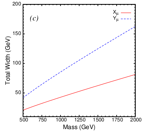
With the knowledge of the decay modes of the leptoquark gauge bosons and the branching fractions for the decays we can now analyze all the different final states that we expect from the pair production of these leptoquarks at the LHC. Note that the total decay widths () for the leptoquark gauge bosons are such that and we have therefore used the narrow width approximation (NWA) which proves to be a useful tool in simplifying the analysis without introducing large errors [25]. We have fixed the coupling to the value of the strong coupling constant () throughout the analysis.
III.3 Signals at LHC
In Ref.[18] we studied the signals for the pair production of the leptoquark gauge bosons and their subsequent decays into the dominant mode at LHC center of mass energies of 7 TeV and 8 TeV. The final state signal was with all the four particles being detected in the respective flavor tagged mode. It was observed that the signal stands out as resonances in the invariant mass distribution of the lepton paired with the jets against the continuum SM background, provided all the four final state particles carried significant transverse momenta. Using this signal a phenomenological prediction on the LHC reach was made on the mass of the which has subsequently been estimated as 760 GeV at 95 % C.L. by the CMS Collaboration [23] at LHC with 7 TeV center of mass energy. As our model predicts another decay mode (to top quark pairs) for the gauge boson, where the behaves as a diquark, carrying quantum numbers of two quarks, it is of extreme importance to be able to highlight this characteristic which distinguishes this particle from the usual leptoquark particles. Establishing the existence of both decay modes is needed to show that these interactions are both baryon and lepton number violating. It is also worth pointing out that a similarly massive in the spectrum which couples as strongly to the gluons as the will also be produced with similar rates and needs to be studied in tandem with the production of the particles at the LHC.
We now consider all decay modes of both the and and discuss final states which is then studied against the SM backgrounds. For the pair production process of gauge bosons, where we have the following different final states given as
| (34) |
The top quark would further decay, either semileptonically or hadronically to give multi-lepton and high jet multiplicity final states. For our purposes, if we assume that the top quarks could be reconstructed with some reasonable efficiency in either modes, we can just focus on the above mentioned final state signal. Similarly for the pair production of the gauge bosons, where we get the following set of final states given as
| (35) |
Note that both the and gauge boson productions at the LHC leads to a rich range of diverse final states which lead to many multi-particle signals and would lead to distinct resonances in the invariant mass distributions in some pairs corresponding to the mass of the and states. Notably we find that each particular event rate is fixed once the model parameters have been fixed, which in our case is the mass of the leptoquark gauge bosons while its coupling strength to the gluons has been fixed to be the strong coupling constant. Thus the success of the model is not dependent on an observation in only one particular final state but that observation needs to be complemented simultaneously in various other channels as listed above in Eqs.(34) and (35). Thus the study on all simultaneous channels deserves merit as it will be able to confirm or falsify the model in question.
We now consider different final states and analyze the signals against the SM background. As we expect that the new gauge bosons when produced on-shell will decay to specific final state products, this would lead to a bump in the invariant mass distribution of the decay products. Keeping this in mind, it is instructive to first consider the most likely signals where the resonances would be observable. Based on the decay channels and final states listed in Eqs.(34)–(35) one should consider the () mode for the gauge bosons while the ( and ) mode looks the more promising for the resonance searches. The other modes either involve neutrinos or more than a single top quark in the final state, which further decays either semileptonically or hadronically and therefore makes it more tasking to reconstruct the leptoquark gauge boson mass. However, we must emphasize that for measuring the electric charge of these gauge bosons one definitely requires that the resonance is observed in the invariant mass distribution of same-sign top quark pair () while the resonance is observed in the () final state or its charge conjugate mode. Notwithstanding the fact that reconstructing the state would be challenging, it would definitely lead to a very interesting observation. Final states involving jets require measuring the jet charge which looks to be more difficult and hence not a desired mode to get information on the charge of the exotic gauge bosons.
| – | |||
In Table 2 we list the relevant SM background subprocesses that we have considered for each set of final states for the signal. Note that we do not make a distinction between the and but we distinguish between a and by assuming exact charge measurement will be possible. We also distinguish between a top quark and anti-top quark assuming that they will be reconstructed with their respective charge identifications from its semileptonic decay modes. We associate an efficiency factor of with this reconstruction. For final state signals not involving neutrinos we have not considered SM subprocesses with as they will involve extra electroweak vertices which suppress the contributions and further requirements on missing transverse momenta would make these contributions too small to take into further consideration. We highlight the above mentioned invariant mass distributions in our model for a few choices of the and gauge boson masses considered at two different center of mass energies for the LHC. We focus our attention to the recently concluded 8 TeV run and the proposed upgrade in energy of 14 TeV for the LHC. As a current limit of 760 GeV exists on the leptoquark gauge boson mass from the CMS analysis [23] we choose a mass of 800 GeV to show the distributions at the 8 TeV run of LHC while a larger mass of 1 TeV is chosen to highlight the signal distributions at the 14 TeV run. We note that there are more than one set of final states where a particular resonance could be observed in the invariant mass distributions and so we consider the scenario where we look at a few definite invariant mass distributions in individual final state modes listed in Eqs.(34) and (35). We list below the pair of final state particles for which the invariant mass distribution is considered, motivated by favored modes for reconstructing the mass and the charge of the and gauge bosons.
- (C1)
Invariant mass distribution of coming from the final states . This is the most favorable mode for reconstructing the resonance.
- (C2)
Invariant mass distribution of same sign top quark pair coming from the final states . The reconstruction of the leptoquark mass in this mode, although difficult, is essential in measuring the charge of the .
- (C3)
Invariant mass distribution of coming from the final states . This is one of the favorable modes for reconstructing the resonance.
- (C4)
Invariant mass distribution of coming from the final states . This mode is essential to measure the charge of the . Note that the resonance corresponds to the charge conjugate mode of .
We shall now discuss the signal and the associated SM backgrounds for the list of resonances given by C1–C4. Note that the signal subprocesses which contribute to give a final state as listed in (C1) come from both and pair productions. However the resonant distribution only happens for the production while the contribution acts to smear out the resonance although it does contribute in enhancing the signal over the SM background. A further smearing effect would come if the signal is included. But we can reject that contribution by demanding that we don’t include events with large missing transverse momenta in the final state when reconstructing the invariant mass. As discussed in Ref.[18] the dominant background for the resonant signal in the channel comes from where when we consider the signal coming from the pair production of which then decay in the mode to give a final state. The light jet final states in the SM can be mistaged as or jets and thus form a significant source for the background due to the large cross sections at LHC, as they are dominantly produced through strong interactions. Guided by previous analysis [18], we note that a very strong requirement on the transverse momenta for the jet and the lepton is very helpful in suppressing the SM background. The SM background has been estimated using Madgraph 5 [26]. In this analysis we further restrict the number of SM background sub-processes that contribute to the final state with by demanding that the tau charge is measured. Therefore we neglect the contributions coming from jets that fake a tau. For example, when we consider the final state as and demand that the tau lepton is tagged as well as its charge measured, we include as the dominant SM processes for the background.
We have used two values for the leptoquark gauge boson () masses, GeV at LHC with center of mass energy 8 TeV and TeV at LHC with center of mass energy 14 TeV to highlight the signal cross sections and differential distributions for invariant mass. We set the factorization and renormalization scale () to the mass of the boson and also use the strong coupling constant value of evaluated at the boson mass. Note that we have evaluated the individual signals as listed in Eqs.(34) and (35) against their specific backgrounds independently. We have assumed in our analysis that the top quark and the anti-top quark are reconstructed with good efficiencies which we can parameterize as . Note that we have used the following efficiencies for and tagging, while we assume a mistag rate for light jets to be tagged as jets as 1% and jets tagged as jets to be 10%. All our results here are done at the parton level and therefore to account for the detector resolutions for energy measurement of particles, we have used a Gaussian smearing of the jet and energies with an energy resolution given by and respectively when analyzing the signal events.
In Table 3 we list the kinematic selection cuts on the events. As the primary decay modes of the heavy leptoquark gauge bosons will have very large transverse momenta we put strong cuts on them. This helps in suppressing the SM background while it does not have any significant effect on the signal events. The cuts on applies only to final states with neutrinos in the decay chain while the cut is on any pair of visible particles. The invariant mass cut is on any pair of jets in the final state.
| Variable | Cut at 8 TeV | Cut at 14 TeV |
|---|---|---|
| GeV | GeV | |
| GeV | GeV | |
| GeV | GeV |
With the above set of kinematic selection on the final state events we evaluate the signal cross sections and the corresponding SM background given in Table 2. We first consider the resonance given by (C1) and show the invariant mass distribution of in Fig. 4. We must point out here that the is paired with the jet which has the leading transverse momenta in case there exist more than one tagged jets. After including the efficiency factors and associated with tagging the and jets and mistag rates, we estimate the signal cross section in the mode as for GeV at LHC with TeV and


for TeV at LHC with TeV. In Fig.4 we plot the invariant mass distribution for the signal. The dominant SM background are given by the following subprocesses, and which after including the efficiency factors, mistag rates is added to give . This is plotted in Fig.(4) as “SM ”. The corresponding SM background at 14 TeV center of mass energy is much more suppressed () because of the strong requirement on the transverse momenta of the jets and the charged tau leptons. The signal is clearly seen to stand out as resonance and one therefore expects this particular mode to be very favorable in searching for the resonance by suppressing the SM background by demanding lepton charge identification which gets rid of the large all jet background. Another mode for the resonance which has completely negligible SM background, is for the final state . There are two different sources for the signal in this case, one which corresponds to the final states coming from the pair production while the other from the pair production. As the contribution does not lead to a resonance in the mode, it will act to smear out the resonance as compared to that seen for the final state. This is evident in Fig.(4) where the width of the resonance is seen to spread out in more invariant mass bins for the final state. Assuming a top reconstruction with an efficiency of we find that the signal cross section from for GeV at LHC with TeV is while the signal cross section from for GeV at LHC with TeV is . Note that the and tagging efficiencies have been already included. In Fig.(4) we have assumed for illustration purposes. Therefore the efficacy of the signal with the same sign top pairs in the final state is dependent on the inherent purity of the top reconstruction at experiments.
We now consider the resonance given by (C2) and show the invariant mass distribution of the same sign top pair in Fig. (5). As pointed out earlier, this mode is necessary to measure the charge of the leptoquark gauge boson mass. A resonant bump in the same sign top pair invariant mass distribution would be a clear indication of a particle decaying into two same sign top quarks and therefore give a strong indication that the particle carries 4/3 electric charge and has quantum numbers of a diquark.


The signal is again considered for two different set of final states, both of which show an invariant mass peak in the same sign top quark pair. In the final state the signal cross section comes solely from the pair production of the gauge bosons. As we have assumed a reconstruction efficiency for the top quarks as , the cross section for GeV at LHC with TeV is . The SM background for the same subprocess is at LHC with TeV. Although the strength of the signal crucially depends on the reconstruction efficiency, even a low efficiency in the long run will lead to a very important observation provided similar resonances are observed in the or final states. The other final state which shows a bump in invariant mass is and its strength was already discussed for Fig.(4). Note that again the contribution does not help the resonance, but is effective in enhancing the signal in this mode.


We now look at the final states which correspond to resonant signals for the gauge boson. We therefore consider the resonance given by (C3) and show the invariant mass distribution of the top-bottom pair in Fig.(6). Note that one of the dominant decay mode for the gauge boson gives neutrinos in the final states that leads to large missing transverse energy (MET) and is not suitable to reconstruct the mass. However, allowing one to decay in the neutrino mode still allows reconstruction of the other in the visible decay modes of and . A large MET in the final state also helps in suppressing large contributions to the SM background through all hadronic final states which proceed through strong interactions. In Fig.(6) we consider four different final state signals which lead to a resonance in the invariant mass, namely and . The signal remains the same as discussed for Fig.(4) with the only difference being that the contribution coming from the pair production now acts to smear out the resonance in invariant mass distribution coming from the . This is the cleanest mode with practically no SM background, although depending on the reconstruction of the top quarks. The signal cross section for the final state comes from the pair production and for GeV at LHC with TeV is . The SM background at LHC with TeV for the signal comes dominantly from three subprocesses with and . The stronger cuts at the 14 TeV run is responsible for the relatively smaller numbers for the SM background for the higher energy run. Note that after including the tagging efficiencies and misstag rates, the corresponding SM background for the final state comes out to be . Although the SM backgrounds are large in this case, the differential cross section is seen to fall rapidly for larger values of the invariant mass. Therefore, a strong cut on the invariant mass will be useful to suppress the background further. For the two final states involving missing transverse energy, we have combined their contribution in Fig.(6) under the signal “”. We find that the SM background for is completely negligible. Note that in the SM background for “”, Fig.(6b) shows an unusual kink in the invariant mass distribution of . This is a kinematical effect driven by the strong kinematic cuts that we put on the final states. The contribution to final state events for can be isolated into dominant contributions coming from the on-shell production of and contributions where a -jet is recoiling against a system ( scattering). The strong requirement on the GeV of the final products suppresses the contributions more while affecting the less which leads to the kink in the invariant mass distribution. A much weaker requirement of GeV (as is the case with TeV) or lower leads to complete amelioration of the kink like behavior and the SM background distribution looks very similar to that in Fig.(6a). The large contribution to the background comes from the at LHC with TeV, while the and are much suppressed due to the small CKM mixings between the first two generation quarks and the top quark. The SM background after including the efficiency factors is then given as , while the signal for GeV at the two center of mass energies is and . Note that is the one which gives a resonant signal while gives a continuum in the invariant mass distribution because the and come from different . This can be seen in Fig.(6) where the large signal contribution in the channel is spread out in the invariant mass distribution. Therefore it is instructive to put a veto on the signal with missing transverse momenta when looking at the invariant mass distribution in . Again for illustrative purposes we have chosen .
We finally consider the resonance given by (C4) which again is essential in measuring the charge of the gauge boson. To measure the charge one requires the charge measurement of the lepton as well as the reconstruction of the top quark in its semileptonic channel. We therefore show the invariant mass distribution in the reconstructed top quark and charged tau lepton pair in Fig.(7) which corresponds to a resonance for the charge conjugated field of .


The signal is obtained from three different set of final states given by and . As discussed before the contribution is found to have negligible SM background but the contribution from the production to the invariant mass distribution itself acts as a background for the resonant signal from the production. The signal comes solely from the pair production and we find that with the proper charge identification of the leptons, we can ignore contributions from SM background processes such as . The signal cross section in this mode is found to be for GeV at LHC with TeV. The SM background is quite suppressed at both center of mass energy values, given by . The signal discussed for the resonance in Fig.(6) was found to give a continuum distribution in the invariant mass. However it leads to a resonance in the invariant mass distribution as . The event rates are the same as before but one can clearly see a distinct resonance confined to a few bins in the invariant mass distribution of in Fig.(7) for the signal. The large SM background for this mode can again be suppressed with a significantly strong cut on the invariant mass. Note again that for the SM background for the invariant mass distribution at TeV, a similar kink like feature is observed in Fig.(7b). This is because the same subprocess which contributes in Fig.(6b) also features in this case with similar kinematic cuts which we have already discussed before. We must however point out that if strong requirements for the final products were put on events for TeV, we get a similar kink like behavior in the invariant mass distribution.
III.4 LHC sensitivity to the and gauge bosons
As evident from our analyses of the resonant signals for the and gauge bosons in our models, the LHC would be able to see the signals in various different channels for significantly large values of their mass. A single channel analysis in the mode relevant for search was considered for its search at the 7 TeV run of LHC [18, 23] while another experimental study relevant for the search in the channel has been done by the CMS Collaboration [27]. Here we do a more expansive sensitivity reach at the LHC for these gauge bosons that can be obtained at different integrated luminosities. For the top decaying semileptonically to where the events will be at most, or less than of the reconstructed top events. While it would be in the hadronic decay mode. Thus it gives a clear demarcation on the event rate we specify for the final states involving the top and anti-top quarks that would lead to any signal events to reconstruct the tops.
For the sensitivity analysis we define the signal to be observable if the lower limit on the signal plus background is larger than the corresponding upper limit on the background [28] with statistical fluctuations
or equivalently,
| (36) |
where is the integrated luminosity, is the signal cross section, and is the background cross section. The parameter specifies the level or probability of discovery. We take , which corresponds to a signal. For , this requirement becomes similar to
| (37) |
where is the number of events for the signal, is the number of events for the background, and equals the statistical significance.
| 0.12 (0.002) | – | ||
| 2.31 (24.34) | 0.35 (0.04) | ||
| 15.18 (9.65) | 25.06 (3.83) | ||
| 22.16 (0.75) | 22.16 (0.75) | ||
| 0.003 (0.001) | 0.001 (0.0006) |
In Table 4, we have calculated the SM background for the different final states that we have considered for the signal coming form the pair productions of the and gauge bosons. The cross sections shown in Table 4 are obtained after passing the events through the kinematic selection conditions given in Table 3. In most cases the SM backgrounds are quite small and would remain negligible even with an integrated luminosity of 100 fb-1. Note that as the top reconstruction would require sufficient events after it has decayed, we need much larger cross sections for the final states involving top quarks. To use Eq.(36), we require the background events to be sufficiently large such that the fluctuations to a Gaussian distribution could be applied. We find that the best reaches are obtained for the and final states. For the final state at LHC with TeV, the signal cross section for a sensitivity must be greater than for an integrated luminosity of respectively. This corresponds to the mass reach of GeV respectively. With the higher center of mass energy option for LHC with TeV, the signal cross section for a sensitivity must be greater than for an integrated luminosity of respectively. These lead to a mass reach of GeV respectively. For the other channels involving the top quark in the final state, we assume the reconstruction efficiency for the top quark which includes the event loss from kinematic cuts after the top decays. Adding the contributions for and we find that at the 8 TeV run of LHC, the mass reach is GeV for an integrated luminosity of respectively while at the 14 TeV run of LHC, where we use the high luminosity options of and , the sensitivity comes out to be about GeV and GeV respectively.
IV Summary and Conclusions
Although the Standard Model, based on local gauge symmetries, accidentally conserve baryon and lepton numbers, there is no fundamental reason for the baryon and lepton numbers to be exact symmetries of Nature. In fact, Grand Unification, unifying quarks and leptons, naturally violate baryon and lepton number. The remarkable stability of the proton dictate that the masses of these leptoquark and diquark gauge bosons to be at the GeV scale. However, baryon and lepton number violating interaction involving only the 3rd family of fermions is not much constrained experimentally. Inspired by the topcolor, topflavor and top hypercharge models, we have a top-GUT model where only the third family of fermions are unified in an with the symmetry breaking scale at the TeV. These models give baryon and lepton number violating gauge interactions which involve only the third family, and with interesting resonant signals at the LHC.
We have proposed two models, the minimal and renormalizable top where the gauge symmetry is broken down to the Standard Model (SM) gauge symmetry via the bifundamental Higgs fields at low energy. The first two families of the SM fermions are charged under while the third family is charged under . In the minimal top model, we showed that the quark CKM mixing matrix can be generated via dimension-five operators, and the proton decay problem can be solved by fine-tuning the coefficients of the high-dimensional operators at the order of . In the renormalizable top model, we introduced additional vector-like fermions whose renormalizable interactions with the SM particles generate these dimension 5 interactions and we can explain the quark CKM mixing matrix by introducing the vector-like particles, and also there is no proton decay problem. We have discussed the phenomenology of the models in details looking for the resonant signals for the baryon and lepton number violating leptoquark as well as diquark gauge bosons at the LHC, as well as the various final state arising from the productions and decays of these heavy gauge bosons. We have also calculated the corresponding SM backgrounds. We find that a signal can be observed for a mass leptoquark / diquark of about 770/800 GeV at the 8 TeV LHC with luminosity of / . The mass reach extends to about 1450 TeV for 14 TeV LHC with a luminosity of .
Acknowledgements.
This research was supported in part by the Natural Science Foundation of China under grant numbers 10821504, 11075194, and 11135003, and by the United States Department of Energy Grant Numbers DE-FG03-95-Er-40917, DE-FG02-04ER41306. The work of S.K.R. was partially supported by funding available from the Department of Atomic Energy, Government of India, for the Regional Centre for Accelerator-based Particle Physics, Harish-Chandra Research Institute.References
- [1] T. D. Lee and C. N. Yang, Phys. Rev. 128, 885 (1962).
- [2] G. ’t Hooft, Nucl. Phys. B 33, 173 (1971); G. ’t Hooft and M. J. G. Veltman, Nucl. Phys. B 50, 318 (1972).
- [3] B. W. Lee and J. Zinn-Justin, Phys. Rev. D 5, 3121 (1972); Phys. Rev. D 5, 3137 (1972); Phys. Rev. D 5, 3155 (1972); Phys. Rev. D 7, 1049 (1973).
- [4] C. T. Hill, Phys. Lett. B 266, 419 (1991); Phys. Lett. B 345, 483 (1995).
- [5] C. T. Hill and S. J. Parke, Phys. Rev. D 49, 4454 (1994).
- [6] D. A. Dicus, B. Dutta and S. Nandi, Phys. Rev. D 51, 6085 (1995).
- [7] D. J. Muller and S. Nandi, Phys. Lett. B 383, 345 (1996).
- [8] E. Malkawi, T. Tait and C. P. Yuan, Phys. Lett. B 385, 304 (1996).
- [9] J. Erler, P. Langacker and T. Li, Phys. Rev. D 66, 015002 (2002), and references therein.
- [10] C. -W. Chiang, J. Jiang, T. Li and Y. -R. Wang, JHEP 0712, 001 (2007) [arXiv:0710.1268 [hep-ph]].
- [11] J. C. Pati and A. Salam, Phys. Rev. D 10, 275 (1974); R. N. Mohapatra and J. C. Pati, Phys. Rev. D 11, 566 (1975); G. Senjanovic and R. N. Mohapatra, Phys. Rev. D 12, 1502 (1975).
- [12] H. Georgi and S. L. Glashow, Phys. Rev. Lett. 32, 438 (1974).
- [13] H. Georgi, Particles and Fields, 1974 (APS/DPF Williamsburg), ed. C. E. Carlson (AIP, New York, 1975) p.575; H. Fritzsch and P. Minkowski, Annals Phys. 93, 193 (1975).
- [14] T. Li and S. Nandi, Phys. Lett. B 617, 112 (2005) [hep-ph/0408160].
- [15] T. Li, Phys. Lett. B 520, 377 (2001) [hep-th/0107136].
- [16] T. Li and W. Liao, hep-th/0207126; Mod. Phys. Lett. A 17, 2393 (2002).
- [17] J. Jiang, T. Li and W. Liao, J. Phys. G G 30, 245 (2004) [hep-ph/0210436].
- [18] S. Chakdar, T. Li, S. Nandi and S. K. Rai, Phys. Lett. B 718, 121 (2012) [arXiv:1206.0409 [hep-ph]].
- [19] G. Aarons et al. [ILC Collaboration], arXiv:0709.1893 [hep-ph].
- [20] L. Linssen, A. Miyamoto, M. Stanitzki and H. Weerts, arXiv:1202.5940 [physics.ins-det].
- [21] J. Blumlein, E. Boos and A. Kryukov, Z. Phys. C 76, 137 (1997); A. Belyaev, C. Leroy, R. Mehdiyev and A. Pukhov, JHEP 0509, 005 (2005).
- [22] J. Pumplin, D. R. Stump, J. Huston, H. L. Lai, P. M. Nadolsky and W. K. Tung, JHEP 0207, 012 (2002) [hep-ph/0201195].
- [23] S. Chatrchyan et al. [CMS Collaboration], arXiv:1210.5629 [hep-ex].
- [24] P. Langacker, Phys. Rept. 72, 185 (1981).
- [25] D. Berdine, N. Kauer and D. Rainwater, Phys. Rev. Lett. 99, 111601 (2007) [hep-ph/0703058].
- [26] J. Alwall, et.al., J. High Energy Phys. 06 (2011) 128.
- [27] S. Chatrchyan et al. [CMS Collaboration], JHEP 1212, 055 (2012) [arXiv:1210.5627 [hep-ex]].
- [28] J. Sayre, D. A. Dicus, C. Kao and S. Nandi, Phys. Rev. D 84, 015011 (2011) [arXiv:1105.3219 [hep-ph]].