跳到论文正文
W Papers独立论文阅读器 arXiv:1302.6896 论文正文 计算阅读时间 · 0%
引用这篇论文根据当前论文元数据生成,正式投稿前建议核对。


License: arXiv.org perpetual non-exclusive license
arXiv:1302.6896v3 [math.NA] 21 Nov 2013

Adaptive Finite Element Approximations for Kohn-Sham Models Thanks: This work was partially supported by the Funds for Creative Research Groups of China under grant 11021101, the National Basic Research Program of China under grant 2011CB309703, the National Science Foundation of China under grants 11101416 and 91330202, the National 863 Project of China under grant 2012AA01A309, and the National Center for Mathematics and Interdisciplinary Sciences of Chinese Academy of Sciences.

Huajie Chen ††thanks: Department of Mathematics, Technische Universität München, Germany (chenh@ma.tum.de).    Xiaoying Dai ††thanks: LSEC, Institute of Computational Mathematics and Scientific/Engineering Computing, Academy of Mathematics and Systems Science, Chinese Academy of Sciences, China (daixy@lsec.cc.ac.cn).    Xingao Gong ††thanks: Department of Physics, Fudan University, Shanghai 200433, China (xggong@fudan.edu.cn).    Lianhua He ††thanks: LSEC, Institute of Computational Mathematics and Scientific/Engineering Computing, Academy of Mathematics and Systems Science, Chinese Academy of Sciences, China (helh@lsec.cc.ac.cn).    Aihui Zhou ††thanks: LSEC, Institute of Computational Mathematics and Scientific/Engineering Computing, Academy of Mathematics and Systems Science, Chinese Academy of Sciences, China (azhou@lsec.cc.ac.cn).
Abstract

The Kohn-Sham model is a powerful, widely used approach for computation of ground state electronic energies and densities in chemistry, materials science, biology, and nanoscience. In this paper, we study adaptive finite element approximations for the Kohn-Sham model. Based on the residual type a posteriori error estimators proposed in this paper, we introduce an adaptive finite element algorithm with a quite general marking strategy and prove the convergence of the adaptive finite element approximations. Using Dörfler’s marking strategy, we then get the convergence rate and quasi-optimal complexity. We also carry out several typical numerical experiments that not only support our theory, but also show the robustness and efficiency of the adaptive finite element computations in electronic structure calculations.

Keywords: Kohn-Sham density functional theory, nonlinear eigenvalue problem, adaptive finite element approximation, convergence, complexity.

AMS subject classifications: 35Q55, 65N15, 65N25, 65N30, 81Q05.

1 Introduction

The Kohn-Sham density functional model is a powerful, widely used approach for computation of ground state electronic energies and densities in chemistry, materials science, biology, and nanosciences. Consider a molecular system consisting of MM nuclei of charges {Z1,⋯,ZM}\{Z_{1},\cdots,Z_{M}\} located at the positions {𝐑1,⋯,𝐑M}\{{\bf R}_{1},\cdots,{\bf R}_{M}\} and NN electrons in the non-relativistic and spin-unpolarized setting. By density functional theorem (DFT) [35, 36], the ground state solutions of the system may be obtained by solving the lowest NN eigenpairs of the following Kohn-Sham equation

{(−12​Δ+Vext​(x)+12​∫ℝ3ρ⁡(y)|x−y|​𝑑y+Vxc​(ρ))​ϕi=μi​ϕiin​ℝ3,i=1,2,⋯,N,∫ℝ3ϕi​ϕj=δi​j,\displaystyle\left\{\begin{array}[]{rcl}\left(-\frac{1}{2}\Delta+V_{\rm ext}(x)+\frac{1}{2}\int_{\mathbb{R}^{3}}\frac{\rho(y)}{|x-y|}dy+V_{\rm xc}(\rho)\right)\phi_{i}&=&\mu_{i}\phi_{i}\quad\mbox{in}~\mathbb{R}^{3},\quad i=1,2,\cdots,N,\\[4.30554pt] \displaystyle\int_{\mathbb{R}^{3}}\phi_{i}\phi_{j}&=&\delta_{ij},\end{array}\right.

where Vext(x)=−∑k=1MZk|x−𝐑k|\displaystyle V_{\rm ext}(x)=-\sum_{k=1}^{M}\frac{Z_{k}}{|x-{\bf R}_{k}|} is the electrostatic potential generated by the nuclei, ρ⁡(x)=∑i=1N|ϕi​(x)|2\displaystyle\rho(x)=\sum_{i=1}^{N}|\phi_{i}(x)|^{2} is the electron density, and Vxc​(ρ)V_{\rm xc}(\rho) denotes the exchange-correlation potential.

Since the core electrons do not participate in the chemical binding and remain almost unchanged, a pseudopotential approximation is usually resorted to in practical computations of the Kohn-Sham equation, which is to replace the Coulomb potential of the nucleus and the effects of the core electrons by an effective ionic potential acting on the valence electrons. Therefore, under the pseudopotential framework, only valence electrons are involved. The pseudopotential consists of two terms: a local component VlocV_{\rm loc} (whose associated operator is the multiplication by the function VlocV_{\rm loc}) and a nonlocal component VnlV_{\rm nl} (an operator whose expression is given in Section 2). The resulted equation is still (1) but Vext​(x)=Vloc​(x)+Vnl​(x)V_{\rm ext}(x)=V_{\rm loc}(x)+V_{\rm nl}(x), NN now being the number of valence electrons, and {ϕi}i=1N\{\phi_{i}\}^{N}_{i=1} being the set of the pseudo-orbitals of the valence electrons.

We understand that the Kohn-Sham approach achieves so far the best balance between accuracy and efficiency among all the different formalisms of electronic structure theory, and simulations of large-scale material systems with Kohn-Sham DFT are still computationally very demanding (say, thousands of electrons or more). As a result, efficient numerical algorithms that can be scalable on parallel computing platforms are desirable to enable DFT calculations at larger scale and for more complex systems. We see that real-space techniques and methods for electronic structure calculations have been derived much attention from scientific and engineering computing communities and remarkably developed during the last two decades, among which the finite element method possesses several significant advantages [6, 26, 46, 47, 56, 57]. Although the finite element method employs more degrees of freedom than that of traditional methods like plane waves and Gaussians, it results in sparse algebraic eigenvalue problems and thus it is scalable on parallel computing platforms due to the strictly local basis functions, it is variational, and it is friendly to implement adaptive refinement approaches. Consequently, the computational accuracy and efficiency of the finite element approximations can be well controlled.

We observe that even in the pseudopotential setting, the eigenfunctions of (1) still vary rapidly around nuclei or chemical bonds [6, 18, 32]. Hence it is also natural to apply adaptive finite element (AFE) approaches to improve the approximation accuracy and reduce the computational cost. Indeed, we see that AFE computations have been quite successfully used in solving Kohn-Sham equations and electronic structure calculations. Tsuchida and Tsukada combined the finite element method with the adaptive curvilinear coordinate approach for electronic structure calculation of some molecules [58, 59]; Shen and Zhang introduced some adaptive tetrahedral finite element disretizations in their theses [51, 63] and calculated several typical molecular systems efficiently [32, 52, 64, 65]; Bylaska et.al used adaptive piecewise linear finite element method on completely unstructured simplex meshes to resolve the rapid variation electronic wave functions around atomic nuclei [10]; Dai et.al designed some parallel adaptive and localization based finite element algorithms for typical quantum chemistry and nanometer material computations containing more than one thousand atoms using tens of hundreds of processors on computer cluster [17, 18, 20, 22]; Gavini et.al constructed a finite element mesh using unstructured coarse-graining technique and computed materials systems [44, 55]; Yang successfully scaled their AFE simulations to over 6000 CPU cores on the Tianhe-1A supercomputer in his thesis [61]. The AFE simulations carried out in this paper also show the robustness and efficiency of the AFE computations in electronic structure calculations. We may refer to [27, 56] and references cited therein for other interesting discussions on adaptive finite element method (AFEM).

We see that it is significant to understand the mechanism of AFE computations, analyze the AFE approximations of Kohn-Sham equations, and give a mathematical justification of the AFE algorithm. We note that the AFE computations are based on some a posteriori error estimators and there are a little work concerning analysis of the a posteriori error estimators and convergence of AFE approximations for DFT. In [14, 15], the authors of this paper considered the nonlinear eigenvalue problems derived from the orbital-free DFT and obtained the convergence and optimal complexity of the AFE algorithm. We understand that the orbital-free DFT is viewed as a simplification of the Kohn-Sham DFT, in which only one eigenpair is involved. In this paper, we shall propose and analyze two AFE algorithms for Kohn-Sham DFT calculations and study the associated convergence and quasi-optimal complexity.

Let us now give an informal description of the main results of this paper. We propose and analyze two AFE algorithms: Algorithm 3.1 and Algorithm 4.1, which are based on the residual type a posteriori error estimators. We show the a posteriori error estimates (see Theorem 9) and prove that

  • •

    Under some reasonable assumptions, all limit points of the AFE approximations of the ground state solutions are ground state solutions (see Theorem 5).

  • •

    Under other reasonable assumptions, some eigenpairs (in particular, ground state solutions) can be well approximated by AFE approximations with some convergence rate (see Theorem 15).

In addition, we also study quasi-optimal complexity of AFE approximations (see Theorem 18).

We mention that Algorithm 3.1 and Algorithm 4.1 may be viewed as some extensions of associated existing algorithms for linear elliptic partial differential equations of second order and have been in fact used for years, for instance, in package RealSPACES (Real Space Parallel Adaptive Calculation of Electronic Structure) of the State Key Laboratory of Scientific and Engineering Computing, Chinese Academy of Sciences. As we see, the numerical analysis for AFE approximation has been also derived much attention from the mathematical community. Since Babuška and Vogelius [4] gave an analysis of an AFEM for linear symmetric elliptic problems in one dimension, there has been much investigation on the convergence and complexity of AFEMs in literature (see, e.g., [9, 12, 21, 23, 30, 53] and the references cited therein). In the context of the finite element approximations of linear eigenvalue problems, in particular, we see that there are a number of works concerning a posteriori error estimates [8, 19, 24, 34, 37, 39, 60], AFEM convergence [21, 29, 30, 31, 33] and complexity [19, 21, 29, 33].

However, there are several crucial difficulties in numerical analysis of the Kohn-Sham equation: it is a nonlinear eigenvalue problem whose eigenvalues may be degenerate, and a number of eigenpairs must be involved; the associated energy functional is nonconvex with respect to density ρ\rho, as a result, there is no uniqueness result for the ground state solutions; the energy functional is invariance under unitary transforms, which also induces redundancy of the ground state solutions. To handle these difficulties arising from the Kohn-Sham equations, we shall present some sophisticated arguments and consider the convergence under the distance between solution sets; investigate the convergence rate and optimal complexity under certain inf-sup assumption; and exploit the relationship between the finite element nonlinear eigenvalue approximations and the associated finite element boundary value approximations. Thanks to our previous works [13, 14, 15, 19, 21, 33, 66, 67] where the perturbation argument was introduced for analyzing AFEM of eigenvalue problems and the compact approach was specialized for handling the nonlinear effects, combining the crucial technical results proposed also in this paper, we are then able to analyze our adaptive finite element algorithms for Kohn-Sham equations, prove the convergence and get the complexity.

The rest of this paper is organized as follows. In Section 2, we provide some preliminaries for Kohn-Sham DFT problem setting and residual type a posteriori error estimator based AFE methods. We prove the convergence of AFE approximations in Section 3 and analyze the convergence rate and optimal complexity of an AFE algorithm in Section 4. In Section 5, we present some numerical experiments that support the theory. Finally, we give some concluding remarks.

2 Preliminaries

Physically, the Kohn-Sham model is set in ℝ3\mathbb{R}^{3}. However, due to the exponential decay of the ground state wavefunction of the Schrödinger equation (c.f., e.g., [2, 62]) and the fact that Kohn-Sham model is an approximation of Schrödinger equation, ℝ3\mathbb{R}^{3} is usually replaced by some polyhedral domain Ω⊂ℝ3\Omega\subset\mathbb{R}^{3} in practical computations for Kohn-Sham equation.

For κ∈ℝN×N\kappa\in\mathbb{R}^{N\times N}, we denote its Frobenius norm by |κ||\kappa|. For p≥1p\geq 1 and s≥0s\geq 0, we denote by Ws,p​(Ω)W^{s,p}(\Omega) the standard Sobolev spaces with the induced norm ∥⋅∥s,p,Ω\|\cdot\|_{s,p,\Omega} (see, e.g. [1, 16]). For p=2p=2, we denote by Hs​(Ω)=Ws,2​(Ω)H^{s}(\Omega)=W^{s,2}(\Omega) with the norm ∥⋅∥s,Ω=∥⋅∥s,2,Ω\|\cdot\|_{s,\Omega}=\|\cdot\|_{s,2,\Omega}, and H01​(Ω)={v∈H1​(Ω):v∣∂Ω=0}H^{1}_{0}(\Omega)=\{v\in H^{1}(\Omega):v\mid_{\partial\Omega}=0\}, where v∣∂Ω=0v\mid_{\partial\Omega}=0 is understood in the sense of trace. The space H−1​(Ω)H^{-1}(\Omega), the dual of H01​(Ω)H^{1}_{0}(\Omega), will also be used. Let ℋ=(H01​(Ω))N\mathcal{H}=(H_{0}^{1}(\Omega))^{N} be the Hilbert space with H1H_{1} inner product

(Φ,Ψ)=∑i=1N∫Ωϕi​ψifor​Φ=(ϕ1,⋯,ϕN),Ψ=(ψ1,⋯,ψN)∈ℋ.(\Phi,\Psi)=\sum_{i=1}^{N}\int_{\Omega}\phi_{i}\psi_{i}\hskip 10.00002pt{\rm for}~\Phi=(\phi_{1},\cdots,\phi_{N}),\Psi=(\psi_{1},\cdots,\psi_{N})\in\mathcal{H}.

Let ℚ\mathbb{Q} be a subspace with orthonormality constraints:

ℚ={Φ∈ℋ:ΦT​Φ=IN×N},\displaystyle\mathbb{Q}=\{\Phi\in\mathcal{H}:\Phi^{T}\Phi=I^{N\times N}\},

where ΦT​Ψ=(∫Ωϕi​ψj)i​j∈ℝN×N\displaystyle\Phi^{T}\Psi=\left(\int_{\Omega}\phi_{i}\psi_{j}\right)_{ij}\in\mathbb{R}^{N\times N}. For Φ∈ℋ\Phi\in\mathcal{H} and a subdomain ω⊂Ω\omega\subset\Omega, we shall denote by ρΦ=∑i=1N|ϕi|2\displaystyle\rho_{\Phi}=\sum_{i=1}^{N}|\phi_{i}|^{2} and (sometimes abuse the notation for simplicity) by

∥Φ∥s,ω=(∑i=1N∥ϕi∥s,ω2)1/2,s=0,1;∥Φ∥0,p,ω=(∑i=1N∥ϕi∥0,p,ωp)1/p,1≤p≤6.\displaystyle\|\Phi\|_{s,\omega}=\left(\sum_{i=1}^{N}\|\phi_{i}\|_{s,\omega}^{2}\right)^{1/2},s=0,1;\hskip 10.00002pt\|\Phi\|_{0,p,\omega}=\left(\sum_{i=1}^{N}\|\phi_{i}\|_{0,p,\omega}^{p}\right)^{1/p},1\leq p\leq 6.

In our discussions, we shall use the following sets:

𝒮N×N={M∈ℝN×N:MT=M},𝒜N×N={M∈ℝN×N:MT=−M}.\mathcal{S}^{N\times N}=\{M\in\mathbb{R}^{N\times N}:M^{T}=M\},~~\mathcal{A}^{N\times N}=\{M\in\mathbb{R}^{N\times N}:M^{T}=-M\}.

For any Φ∈ℚ\Phi\in\mathbb{Q}, we may decompose ℋ\mathcal{H} into a direct sum of three subspaces (see, e.g., [25]):

ℋ=𝒮Φ⊕𝒜Φ⊕𝒯Φ,\displaystyle\mathcal{H}=\mathcal{S}_{\Phi}\oplus\mathcal{A}_{\Phi}\oplus\mathcal{T}_{\Phi},

where 𝒮Φ=Φ​𝒮N×N\mathcal{S}_{\Phi}=\Phi\mathcal{S}^{N\times N}, 𝒜Φ=Φ​𝒜N×N\mathcal{A}_{\Phi}=\Phi\mathcal{A}^{N\times N}, and 𝒯Φ={Ψ∈ℋ:ΨT​Φ=0∈ℝN×N}.\mathcal{T}_{\Phi}=\left\{\Psi\in\mathcal{H}:\Psi^{T}\Phi=0\in\mathbb{R}^{N\times N}\right\}.

For convenience, the symbol ≲\lesssim will be used throughout this paper, and A≲BA\lesssim B means that A≤C​BA\leq CB for some constant CC that is independent of mesh parameters. We use 𝒫⁡(p,(c1,c2))\mathscr{P}(p,(c_{1},c_{2})) to denote a class of functions satisfying some growth conditions:

𝒫(p,(c1,c2))={f:∃a1,a2∈ℝ such that c1tp+a1≤f(t)≤c2tp+a2∀t≥0}\displaystyle\mathscr{P}(p,(c_{1},c_{2}))=~\big\{f:~\exists~a_{1},a_{2}\in\mathbb{R}\mbox{ such that }~c_{1}t^{p}+a_{1}\leq f(t)\leq c_{2}t^{p}+a_{2}\hskip 10.00002pt\forall t\geq 0\big\}

with c1∈ℝc_{1}\in\mathbb{R} and c2,p∈[0,∞)c_{2},p\in[0,\infty).

2.1 Problem setting

Consider the following general form of Kohn-Sham energy functional

E⁡(Φ)\displaystyle E(\Phi) =\displaystyle= ∫Ω(12​∑i=1N|∇ϕi|2+Vloc​ρΦ+∑i=1Nϕi​Vnl​ϕi+exc​(ρΦ))\displaystyle\int_{\Omega}\left(\frac{1}{2}\sum_{i=1}^{N}|\nabla\phi_{i}|^{2}+V_{\rm loc}\rho_{\Phi}+\sum_{i=1}^{N}\phi_{i}V_{\rm nl}\phi_{i}+e_{\rm xc}(\rho_{\Phi})\right) (1)
+12​D​(ρΦ,ρΦ)\displaystyle+\frac{1}{2}D(\rho_{\Phi},\rho_{\Phi})

for Φ=(ϕ1,ϕ2,⋯,ϕN)∈ℋ\Phi=(\phi_{1},\phi_{2},\cdots,\phi_{N})\in\mathcal{H}, which includes the cases of Coulomb potentials and pseudopotential approximations. For the Coulomb potential setting, Vloc=−∑k=1MZk|x−𝐑k|V_{\rm loc}=-\sum_{k=1}^{M}\frac{Z_{k}}{|x-{\bf R}_{k}|} and Vnl=0V_{\rm nl}=0. While for the pseudopotential approximations, VlocV_{\rm loc} is the local part of pseudopotential and VnlV_{\rm nl} is a nonlocal pseudopotential operator (see, e.g., [40]) given by

Vnl​ϕ=∑j=1n(ϕ,ζj)​ζjV_{\rm nl}\phi=\sum_{j=1}^{n}(\phi,\zeta_{j})\zeta_{j}

with ζj∈L2​(Ω)​(j=1,2,⋯,n)\zeta_{j}\in L^{2}(\Omega)(j=1,2,\cdots,n), n∈ℕn\in\mathbb{N}. D⁡(ρΦ,ρΦ)D(\rho_{\Phi},\rho_{\Phi}) is the electron-electron Coulomb energy defined by

D⁡(f,g)=∫Ωf⁡(g∗r−1)=∫Ω∫Ωf⁡(x)​g​(y)​1|x−y|​𝑑x​𝑑y,D(f,g)=\int_{\Omega}f(g*r^{-1})=\int_{\Omega}\int_{\Omega}f(x)g(y)\frac{1}{|x-y|}dxdy,

and exc​(t)e_{\rm xc}(t) is some real function over [0,∞)[0,\infty). In our analysis, we require VlocV_{\rm loc} belongs to L2​(Ω)L^{2}(\Omega). We point out that Vloc∈L2​(Ω)V_{\rm loc}\in L^{2}(\Omega) is a very mild condition, which is satisfied by both the Coulomb potential Vext(x)=−∑k=1MZk|x−𝐑k|V_{\rm ext}(x)=-\sum_{k=1}^{M}\frac{Z_{k}}{|x-{\bf R}_{k}|} and the local part of pseudopotential. Since exc:[0,∞)→ℝe_{\rm xc}:[0,\infty)\rightarrow\mathbb{R} does not have a simple analytical expression, we shall use some approximations and assume throughout this paper that

exc​(t)∈𝒫⁡(3,(c1,c2))​with​c1≥0orexc​(t)∈𝒫⁡(4/3,(c1,c2)),\displaystyle e_{\rm xc}(t)\in\mathscr{P}(3,(c_{1},c_{2}))~{\rm with}~c_{1}\geq 0\hskip 10.00002pt{\rm or}\hskip 10.00002pte_{\rm xc}(t)\in\mathscr{P}(4/3,(c_{1},c_{2})), (2)

which is satisfied by almost all the LDAs.

The ground state of the system is obtained by solving the minimization problem

inf{E⁡(Φ):Φ∈ℚ},\displaystyle\inf\left\{E(\Phi):\Phi\in\mathbb{Q}\right\}, (3)

and we refer to [3, 11, 13] for the discussion of existence of a minimizer. Note that the energy functional (1) is invariant with respect to any unitary transform, i.e.

E⁡(Φ)=E⁡(Φ​U)=E⁡((∑j=1Nui​j​ϕj)i=1N)∀U=(ui​j)i,j=1N∈𝒪N×N,\displaystyle E(\Phi)=E(\Phi U)=E\big((\sum_{j=1}^{N}u_{ij}\phi_{j})_{i=1}^{N}\big)\hskip 10.00002pt\forall~U=(u_{ij})_{i,j=1}^{N}\in\mathcal{O}^{N\times N}, (4)

where 𝒪N×N\mathcal{O}^{N\times N} is the set of orthogonal matrices. It follows from (4) that if Φ\Phi is a minimizer of (3), then Φ​U\Phi U is also a minimizer for any orthogonal matrix UU. For any Ψ∈ℋ\Psi\in\mathcal{H}, we define the equivalence class

[Ψ]={ΨU,∀U∈𝒪N×N}.\displaystyle[\Psi]=\{\Psi U,~\forall~U\in\mathcal{O}^{N\times N}\}.

We see that any minimizer Φ=(ϕ1,⋯,ϕN)\Phi=(\phi_{1},\cdots,\phi_{N}) of (3) satisfies the following weak form (i.e. the Euler-Lagrange equation associated with the minimization problem):

{(HΦ​ϕi,v)=(∑j=1Nλi​j​ϕj,v)∀v∈H01​(Ω),i=1,2,⋯,N,∫Ωϕi​ϕj=δi​j,\displaystyle\left\{\begin{array}[]{rcl}(H_{\Phi}\phi_{i},v)&=&\displaystyle\big(\sum_{j=1}^{N}\lambda_{ij}\phi_{j},v\big)\quad\forall~v\in H_{0}^{1}(\Omega),\quad i=1,2,\cdots,N,\\[4.30554pt] \displaystyle\int_{\Omega}\phi_{i}\phi_{j}&=&\delta_{ij},\end{array}\right.

where HΦH_{\Phi} is the Kohn-Sham Hamiltonian operator as

HΦ=−12​Δ+Vloc+Vnl+∫ΩρΦ​(y)|⋅−y|​𝑑y+exc′​(ρΦ)\displaystyle H_{\Phi}=-\frac{1}{2}\Delta+V_{\rm loc}+V_{\rm nl}+\int_{\Omega}\frac{\rho_{\Phi}(y)}{|\cdot-y|}dy+e_{\rm xc}^{\prime}(\rho_{\Phi}) (8)

and

Λ=(λi​j)i,j=1N=(∫Ωϕj​HΦ​ϕi)i,j=1N\displaystyle\Lambda=(\lambda_{ij})_{i,j=1}^{N}=\left(\int_{\Omega}\phi_{j}H_{\Phi}\phi_{i}\right)_{i,j=1}^{N} (9)

is the Lagrange multiplier. Since the uniqueness of the ground state solution is unknown even up to a unitary transform, we define the set of ground states by

Θ={(Λ,Φ)∈ℝN×N×ℚ:E(Φ)=minΨ∈ℚE(Ψ)and(Λ,Φ) solves (2.1)}.\displaystyle\Theta=\left\{(\Lambda,\Phi)\in\mathbb{R}^{N\times N}\times\mathbb{Q}:E(\Phi)=\min_{\Psi\in\mathbb{Q}}E(\Psi)~\mbox{and}~(\Lambda,\Phi)\mbox{ solves \eqref{problem-eigen-compact-L}}\right\}. (10)

Note that the electron density ρΦ\rho_{\Phi} and the operator HΦH_{\Phi} are also invariant under any unitary transform, we may diagonalize the matrix of Lagrange multipliers Λ\Lambda. More precisely, there exists a U∈𝒪N×NU\in\mathcal{O}^{N\times N}, such that the Lagrange multiplier is diagonal for Ψ=Φ​U=(ψ1,⋯,ψN)\Psi=\Phi U=(\psi_{1},\cdots,\psi_{N}), i.e.,

∫Ωψj​HΨ​ψi=μi​δi​j.\int_{\Omega}\psi_{j}H_{\Psi}\psi_{i}=\mu_{i}\delta_{ij}.

Consequently, instead of (2.1), we may consider a form with diagonal multiplier as follows:

{(HΨ​ψi,v)=(μi​ψi,v)∀v∈H01​(Ω),i=1,2,⋯,N,∫Ωψi​ψj=δi​j,\displaystyle\left\{\begin{array}[]{rcl}(H_{\Psi}\psi_{i},v)&=&(\mu_{i}\psi_{i},v)\quad\forall~v\in H_{0}^{1}(\Omega),\quad i=1,2,\cdots,N,\\[4.30554pt] \displaystyle\int_{\Omega}\psi_{i}\psi_{j}&=&\delta_{ij},\end{array}\right.

which is the standard Kohn-Sham equation.

Note that any solution of (2.1) can be obtained from a unitary transform of some solution of (2.1). That is, once we get all solution of (2.1), we then obtain all solution of (2.1). Consequently, we also call (2.1) Kohn-Sham equation.

It is well known that the ground state has one electron in each of the NN orbitals with the lowest NN eigenvalues [40]. Therefore, the ground state solutions in (10) can be obtained by solving the lowest NN eigenpairs of (2.1).

For convenience, define ℱ:ℝN×N×ℋ→ℋ∗\mathcal{F}:\mathbb{R}^{N\times N}\times\mathcal{H}\rightarrow\mathcal{H}^{*} by

⟨ℱ⁡(Λ,Φ),Γ⟩=∑i=1N(HΦ​ϕi−∑j=1Nλi​j​ϕj,γi)∀Γ=(γi)i=1N∈ℋ.\displaystyle\langle\mathcal{F}(\Lambda,\Phi),\Gamma\rangle=\sum_{i=1}^{N}\big(H_{\Phi}\phi_{i}-\sum_{j=1}^{N}\lambda_{ij}\phi_{j},\gamma_{i}\big)\hskip 10.00002pt\forall~\Gamma=(\gamma_{i})_{i=1}^{N}\in\mathcal{H}.

The Fréchet derivative of ℱ\mathcal{F} with respect to Φ\Phi at (Λ,Φ)(\Lambda,\Phi) is denoted by ℱΦ′​(Λ,Φ):ℋ→ℋ∗\mathcal{F}_{\Phi}^{\prime}(\Lambda,\Phi):\mathcal{H}\rightarrow\mathcal{H}^{\ast} as follows

⟨ℱΦ′​(Λ,Φ)​Ψ,Γ⟩=14​E′′​(Φ)​(Ψ,Γ)−∑i,j=1N(λi​j​ψj,γi)\displaystyle\langle\mathcal{F}_{\Phi}^{\prime}(\Lambda,\Phi)\Psi,\Gamma\rangle=\frac{1}{4}E^{\prime\prime}(\Phi)(\Psi,\Gamma)-\sum_{i,j=1}^{N}(\lambda_{ij}\psi_{j},\gamma_{i})
=\displaystyle= ∑i=1N(HΦ​ψi−∑j=1Nλi​j​ψj,γi)+4​∑i,j=1N(exc′′​(ρΦ)​ϕi​ψi,ϕj​γj)+∑i,j=1N4​D​(ϕi​ψi,ϕj​γj).\displaystyle\sum_{i=1}^{N}\big(H_{\Phi}\psi_{i}-\sum_{j=1}^{N}\lambda_{ij}\psi_{j},\gamma_{i}\big)+4\sum_{i,j=1}^{N}\big(e_{\rm xc}^{\prime\prime}(\rho_{\Phi})\phi_{i}\psi_{i},\phi_{j}\gamma_{j}\big)+\sum_{i,j=1}^{N}4D(\phi_{i}\psi_{i},\phi_{j}\gamma_{j}).

To study the convergence and complexity, we need the following assumptions [13]

  • A1

    |exc′​(t)|+|t​exc′′​(t)|∈𝒫⁡(p1,(c1,c2))|e_{\rm xc}^{\prime}(t)|+|te_{\rm xc}^{\prime\prime}(t)|\in\mathscr{P}(p_{1},(c_{1},c_{2})) for some p1∈[0,2]p_{1}\in[0,2].

  • A2

    There exists a constant α∈(0,1]\alpha\in(0,1] such that |exc′′​(t)|+|t​exc′′′​(t)|≲1+tα−1∀t>0|e_{\rm xc}^{\prime\prime}(t)|+|te_{\rm xc}^{\prime\prime\prime}(t)|\lesssim 1+t^{\alpha-1}\hskip 10.00002pt\forall~t>0.

  • A3

    (Λ,Φ)(\Lambda,\Phi) is a solution of (2.1) and there exists a constant β>0\beta>0 depending on (Λ,Φ)(\Lambda,\Phi) such that

    infΓ∈𝒯ΦsupΨ∈𝒯Φ⟨ℱΦ′​(Λ,Φ)​Ψ,Γ⟩‖Ψ‖1,Ω​‖Γ‖1,Ω≥β.\displaystyle\inf_{\Gamma\in\mathcal{T}_{\Phi}}\sup_{\Psi\in\mathcal{T}_{\Phi}}\frac{\langle\mathcal{F}_{\Phi}^{\prime}(\Lambda,\Phi)\Psi,\Gamma\rangle}{\|\Psi\|_{1,\Omega}\|\Gamma\|_{1,\Omega}}\geq\beta. (14)
Remark 2.1.

We see that Assumption A2 implies Assumption A1 and the commonly used XαX_{\alpha} and LDA exchange-correlation energy functionals satisfy Assumption A2.

Assumption A3 is equivalent to that ℱΦ′​(Λ,Φ)\mathcal{F}_{\Phi}^{\prime}(\Lambda,\Phi) is an isomorphism from 𝒯Φ\mathcal{T}_{\Phi} to 𝒯Φ\mathcal{T}_{\Phi}. We observe that if Assumption A3 is satisfied for Φ∈ℚ\Phi\in\mathbb{Q}, then Assumption A3 is satisfied for any Φ~∈[Φ]\tilde{\Phi}\in[\Phi] with the same constant β\beta, too. We see that a stronger condition than (14) that

⟨ℱΦ′​(Λ,Φ)​Γ,Γ⟩≥γ​‖Γ‖1,Ω2∀Γ∈𝒯Φ\displaystyle\langle\mathcal{F}^{\prime}_{\Phi}(\Lambda,\Phi)\Gamma,\Gamma\rangle\geq\gamma\|\Gamma\|^{2}_{1,\Omega}\hskip 10.00002pt\forall~\Gamma\in\mathcal{T}_{\Phi}

is used in [11, 50], which is satisfied for a linear self-adjoint operator when there is a gap between the lowest NNth eigenvalue and (N+1)(N+1)th eigenvalue [50].

2.2 Adaptive finite element approximations

Let dΩd_{{}_{\Omega}} be the diameter of Ω\Omega and {𝒯h}\{\mathcal{T}_{h}\} be a shape regular family of nested conforming meshes over Ω\Omega with size h∈(0,dΩ)h\in(0,d_{{}_{\Omega}}): there exists a constant γ∗\gamma^{\ast} such that

hτρτ≤γ∗∀τ∈𝒯h,\displaystyle\frac{h_{\tau}}{\rho_{\tau}}\leq\gamma^{\ast}\hskip 10.00002pt\forall~\tau\in\mathcal{T}_{h}, (15)

where hτh_{\tau} is the diameter of τ\tau for each τ∈𝒯h\tau\in\mathcal{T}_{h}, ρτ\rho_{\tau} is the diameter of the biggest ball contained in τ\tau, and h=max⁡{hτ:τ∈𝒯h}h=\max\{h_{\tau}:\tau\in\mathcal{T}_{h}\}. Let ℰh\mathcal{E}_{h} denote the set of interior faces (edges or sides) of 𝒯h\mathcal{T}_{h}.

Let Sh,k​(Ω)S^{h,k}(\Omega) be a subspace of continuous functions on Ω\Omega such that

Sh,k(Ω)={v∈C(Ω¯):v|τ∈Pτk∀τ∈𝒯h},\displaystyle S^{h,k}(\Omega)=\{v\in C(\bar{\Omega}):~v|_{\tau}\in P^{k}_{\tau}\hskip 10.00002pt\forall~\tau\in\mathcal{T}_{h}\},

where PτkP^{k}_{\tau} is the space of polynomials of degree no greater than kk over τ\tau. Let S0h,k​(Ω)=Sh,k​(Ω)∩H01​(Ω)S^{h,k}_{0}(\Omega)=S^{h,k}(\Omega)\cap H^{1}_{0}(\Omega). We shall denote S0h,k​(Ω)S^{h,k}_{0}(\Omega) by S0h​(Ω)S^{h}_{0}(\Omega) for simplification of notation afterwards and let Vh=(S0h​(Ω))NV_{h}=(S^{h}_{0}(\Omega))^{N}.

We consider the following finite element approximations of (3):

inf{E⁡(Φh):Φh∈Vh∩ℚ}.\displaystyle\inf\{E(\Phi_{h}):\Phi_{h}\in V_{h}\cap\mathbb{Q}\}. (16)

We see from [3, 13] that the minimizer of (16) exists under condition (2) Note that any minimizer Φh=(ϕ1,h,⋯,ϕN,h)\Phi_{h}=(\phi_{1,h},\cdots,\phi_{N,h}) of (16) solves the Euler-Lagrange equation

{(HΦh​ϕi,h,v)=(∑j=1Nλi​j,h​ϕj,h,v)∀v∈S0h​(Ω),i=1,2,⋯,N,∫Ωϕi,h​ϕj,h=δi​j\displaystyle\left\{\begin{array}[]{rcl}(H_{\Phi_{h}}\phi_{i,h},v)&=&\displaystyle\big(\sum_{j=1}^{N}\lambda_{ij,h}\phi_{j,h},v\big)\quad\forall~v\in S^{h}_{0}(\Omega),\quad i=1,2,\cdots,N,\\[4.30554pt] \displaystyle\int_{\Omega}\phi_{i,h}\phi_{j,h}&=&\delta_{ij}\end{array}\right.

with the Lagrange multiplier

Λh=(λi​j,h)i,j=1N=(∫Ωϕj,h​HΦh​ϕi,h)i,j=1N.\displaystyle\Lambda_{h}=(\lambda_{ij,h})_{i,j=1}^{N}=\left(\int_{\Omega}\phi_{j,h}H_{\Phi_{h}}\phi_{i,h}\right)_{i,j=1}^{N}.

Define the set of finite dimensional ground state solutions:

Θh={(Λh,Φh)∈ℝN×N×(ℚ∩Vh):E(Φh)=minΨ∈ℚ∩VhE(Ψ) and (Λh,Φh) solves (2.2)}.\displaystyle\Theta_{h}=\left\{(\Lambda_{h},\Phi_{h})\in\mathbb{R}^{N\times N}\times(\mathbb{Q}\cap V_{h}):E(\Phi_{h})=\min_{\Psi\in\mathbb{Q}\cap V_{h}}E(\Psi)\mbox{ and }(\Lambda_{h},\Phi_{h})\mbox{ solves }\eqref{problem-eigen-compact-dis}\right\}.

We have from [13] that the finite dimensional approximations are uniformly bounded, i.e., there exists a constant CC such that

sup(Λh,Φh)∈Θh,h∈(0,dΩ)(∥Φh∥1,Ω+|Λh|)<C.\displaystyle\sup_{(\Lambda_{h},\Phi_{h})\in\Theta_{h},h\in(0,d_{{}_{\Omega}})}(\|\Phi_{h}\|_{1,\Omega}+|\Lambda_{h}|)<C. (20)

Using a unitary transform, we can diagonalize Λh\Lambda_{h} and obtain a discrete Kohn-Sham equation

{(HΨh​ψi,h,v)=(μi,h​ψi,h,v)∀v∈S0h​(Ω),i=1,2,⋯,N,∫Ωψi,h​ψj,h=δi​j\displaystyle\left\{\begin{array}[]{rcl}(H_{\Psi_{h}}\psi_{i,h},v)&=&(\mu_{i,h}\psi_{i,h},v)\quad\forall~v\in S^{h}_{0}(\Omega),\quad i=1,2,\cdots,N,\\[4.30554pt] \displaystyle\int_{\Omega}\psi_{i,h}\psi_{j,h}&=&\delta_{ij}\end{array}\right.

with μi,h=(HΨh​ψi,h,ψi,h)\mu_{i,h}=(H_{\Psi_{h}}\psi_{i,h},\psi_{i,h}).

Similar to the continuous case, we have that any solution of (2.2) can be obtained from a unitary transform of some solution of (2.2). That is,

Θh={(Λh,Φh)∈ℝN×N×(ℚ∩Vh):Φh∈[Ψh]andΛh=ΦhTHΦhΦh,∀Ψhwith(�h,Ψh)∈Ξh},\displaystyle\Theta_{h}=\left\{(\Lambda_{h},\Phi_{h})\in\mathbb{R}^{N\times N}\times(\mathbb{Q}\cap V_{h}):\Phi_{h}\in[\Psi_{h}]~\mbox{and}~\Lambda_{h}=\Phi_{h}^{T}H_{\Phi_{h}}\Phi_{h},\forall\Psi_{h}~\mbox{with}~(\bbmu_{h},\Psi_{h})\in\Xi_{h}\right\},

where

Ξh={(�h,Ψh)∈ℝN×N×(ℚ∩Vh):E(Ψh)=minΨ∈ℚ∩VhE(Ψ) and (�h,Ψh) solves (2.2)}.\displaystyle\Xi_{h}=\left\{(\bbmu_{h},\Psi_{h})\in\mathbb{R}^{N\times N}\times(\mathbb{Q}\cap V_{h}):E(\Psi_{h})=\min_{\Psi\in\mathbb{Q}\cap V_{h}}E(\Psi)\mbox{ and }(\bbmu_{h},\Psi_{h})\mbox{ solves }(\ref{problem-eigen-dis})\right\}.

Since (2.2) is solvable, to get Θh\Theta_{h}, we always resort to solving (2.2) in practice.

An adaptive mesh-refining algorithm usually consists of the following loop [12, 21]:

Solve→Estimate→Mark→Refine.\mbox{\bf Solve}~\rightarrow~\mbox{\bf Estimate}~\rightarrow~\mbox{\bf Mark}~\rightarrow~\mbox{\bf Refine}.

Solve. This step computes the piecewise polynomial finite element approximation with respect to a given mesh. To simplify the analysis and do as the most work on numerical study of convergence of AFE approximations, we shall assume throughout this paper that we have the exact solutions of discretized problems11 1 Similar conclusion can be expected for the case where the errors of numerical integrations and nonlinear algebraic solvers are included (see Section 6). And we understand that the assumption is indeed a very important practical issue. .

Estimate. Given a partition 𝒯h\mathcal{T}_{h} and the corresponding output (Λh,Φh)(\Lambda_{h},\Phi_{h}) from the “Solve” step, “Estimate” computes the a posteriori error estimator {ηh​(Φh,τ)}τ∈𝒯h\{\eta_{h}(\Phi_{h},\tau)\}_{\tau\in\mathcal{T}_{h}}, which is defined as follows. Define the element residual ℛτ​(Φh)\mathcal{R}_{\tau}(\Phi_{h}) and the jump Je​(Φh)J_{e}(\Phi_{h}) by

ℛτ​(Φh)=(HΦh​ϕi,h−∑j=1Nλi​j,h​ϕj,h)i=1Nin​τ∈𝒯h,\displaystyle\mathcal{R}_{\tau}(\Phi_{h})=\big(H_{\Phi_{h}}\phi_{i,h}-\sum_{j=1}^{N}\lambda_{ij,h}\phi_{j,h}\big)_{i=1}^{N}\hskip 10.00002pt\mbox{in}~\tau\in\mathcal{T}_{h},
Je(Φh)=(je(ϕi,h))i=1N,je(ϕi,h)=12∇ϕi,h|τ1⋅n1→+12∇ϕi,h|τ2⋅n2→,\displaystyle J_{e}(\Phi_{h})=\Big(j_{e}(\phi_{i,h})\Big)_{i=1}^{N},~~j_{e}(\phi_{i,h})=\frac{1}{2}\nabla\phi_{i,h}|_{\tau_{1}}\cdot\overrightarrow{n_{1}}+\frac{1}{2}\nabla\phi_{i,h}|_{\tau_{2}}\cdot\overrightarrow{n_{2}},

where ee is the common face of elements τ1\tau_{1} and τ2\tau_{2} with unit outward normals n1→\overrightarrow{n_{1}} and n2→\overrightarrow{n_{2}}, respectively. Let ωh​(e)\omega_{h}(e) be the union of elements that share the face ee, and ωh​(τ)\omega_{h}(\tau) be the union of elements that share an edge with τ\tau. For τ∈𝒯h\tau\in\mathcal{T}_{h}, we define local error indicator ηh​(Φh,τ)\eta_{h}(\Phi_{h},\tau) and the oscillation osch​(Φh,τ){\rm osc}_{h}(\Phi_{h},\tau) by

ηh2​(Φh,τ)=hτ2​‖ℛτ​(Φh)‖0,τ2+∑e∈ℰh,e⊂∂τhe​‖Je​(Φh)‖0,e2,\displaystyle\eta^{2}_{h}(\Phi_{h},\tau)=h_{\tau}^{2}\|\mathcal{R}_{\tau}(\Phi_{h})\|_{0,\tau}^{2}+\sum_{e\in\mathcal{E}_{h},e\subset\partial\tau}h_{e}\|J_{e}(\Phi_{h})\|_{0,e}^{2},
osch​(Φh,τ)=hτ​‖ℛτ​(Φh)−ℛτ​(Φh)¯‖0,τ,\displaystyle{\rm osc}_{h}(\Phi_{h},\tau)=h_{\tau}\|\mathcal{R}_{\tau}(\Phi_{h})-\overline{\mathcal{R}_{\tau}(\Phi_{h})}\|_{0,\tau},

where w¯\overline{w} is the L2L^{2}-projection of w∈L2​(Ω)w\in L^{2}(\Omega) to polynomials of some degree on τ\tau or ee. Given a subset ω⊂Ω\omega\subset\Omega, we define the error estimator ηh​(Φh,ω)\eta_{h}(\Phi_{h},\omega) and the oscillation osch​(Φh,ω){\rm osc}_{h}(\Phi_{h},\omega) by

ηh2​(Φh,ω)=∑τ∈𝒯h,τ⊂ωηh2​(Φh,τ)andosch2​(Φh,ω)=∑τ∈𝒯h,τ⊂ωosch2​(Φh,τ).\displaystyle\eta^{2}_{h}(\Phi_{h},\omega)=\sum_{\tau\in\mathcal{T}_{h},\tau\subset\omega}\eta^{2}_{h}(\Phi_{h},\tau)\hskip 10.00002pt\mbox{and}\hskip 10.00002pt{\rm osc}^{2}_{h}(\Phi_{h},\omega)=\sum_{\tau\in\mathcal{T}_{h},\tau\subset\omega}{\rm osc}^{2}_{h}(\Phi_{h},\tau).

Mark. We shall replace the subscript hh (or hkh_{k}) by an iteration counter kk whenever convenient afterwards. Based on the a posteriori error indicators {ηk​(Φk,τ)}τ∈𝒯k\{\eta_{k}(\Phi_{k},\tau)\}_{\tau\in\mathcal{T}_{k}}, “Mark” gives a strategy to choose a subset of elements ℳk\mathcal{M}_{k} of 𝒯k\mathcal{T}_{k} for refinement. One of the most widely used marking strategy to enforce error reduction is the so-called Dörfler strategy.

Dörfler Strategy. Given a parameter 0<θ<10<\theta<1 :

  1. 1.

    Construct a subset ℳk\mathcal{M}_{k} of 𝒯k\mathcal{T}_{k} by selecting some elements in 𝒯k\mathcal{T}_{k} such that

    ∑τ∈ℳkηk2​(Φk,τ)≥θ​∑τ∈𝒯kηk2​(Φk,τ).\displaystyle\sum_{\tau\in\mathcal{M}_{k}}\eta^{2}_{k}({\Phi}_{k},\tau)\geq\theta\sum_{\tau\in\mathcal{T}_{k}}\eta^{2}_{k}({\Phi}_{k},\tau). (24)
  2. 2.

    Mark all the elements in ℳk\mathcal{M}_{k}.

A weaker strategy, which is called “Maximum Strategy”, only requires that the set of marked elements ℳk\mathcal{M}_{k} contains at least one element of 𝒯k\mathcal{T}_{k} holding the largest value estimator [29, 30]. Namely, there exists at least one element τkmax∈ℳk\tau^{\max}_{k}\in\mathcal{M}_{k} such that

ηk​(Φk,τkmax)=maxτ∈𝒯k⁡ηk​(Φk,τ).\displaystyle\eta_{k}(\Phi_{k},\tau^{\max}_{k})=\max_{\tau\in\mathcal{T}_{k}}\eta_{k}(\Phi_{k},\tau). (25)

It is easy to check that the most commonly used marking strategies, e.g., Dörfler’s strategy and Equidistribution strategy, fulfill this condition.

Refine. Given the partition 𝒯k\mathcal{T}_{k} and the set of marked elements ℳk\mathcal{M}_{k}, “Refine” produces a new partition 𝒯k+1\mathcal{T}_{k+1} by refining all elements in ℳk\mathcal{M}_{k} at least one time. We restrict ourself to a shape-regular bisection for the refinement. Define

ℛ𝒯k→𝒯k+1=𝒯k\(𝒯k∩𝒯k+1)\displaystyle\mathcal{R}_{\mathcal{T}_{k}\rightarrow\mathcal{T}_{k+1}}=\mathcal{T}_{k}\backslash(\mathcal{T}_{k}\cap\mathcal{T}_{k+1})

as the set of refined elements, we have ℳk⊂ℛ𝒯k→𝒯k+1\mathcal{M}_{k}\subset\mathcal{R}_{\mathcal{T}_{k}\rightarrow\mathcal{T}_{k+1}}. Note that usually more than the marked elements in ℳk\mathcal{M}_{k} are refined in order to keep the mesh conforming.

3 Convergence of adaptive finite element approximations

In this section, we propose and investigate an AFE algorithm with Maximum Strategy for Kohn-Sham equations as follows:

Algorithm 3.1.

AFE algorithm with Maximum Strategy

  1. 1.

    Pick an initial mesh 𝒯0\mathcal{T}_{0}, and let k=0k=0.

  2. 2.

    Solve (2.2) on 𝒯k\mathcal{T}_{k} to get discrete solutions (μi,k,ψi,k)​(i=1,⋯,N)(\mu_{i,k},\psi_{i,k})(i=1,\cdots,N) and then Θk\Theta_{k}.

  3. 3.

    Compute local error indictors ηk​(Ψk,τ)\eta_{k}(\Psi_{k},\tau) for all τ∈𝒯k\tau\in\mathcal{T}_{k}.

  4. 4.

    Construct ℳk⊂𝒯k\mathcal{M}_{k}\subset\mathcal{T}_{k} by Maximum Strategy.

  5. 5.

    Refine 𝒯k\mathcal{T}_{k} to get a new conforming mesh 𝒯k+1\mathcal{T}_{k+1}.

  6. 6.

    Let k=k+1k=k+1 and go to 2.

We shall prove that all the limit points of the AFE approximations generated by Algorithm 3.1 are ground state solutions of (2.1), for which we shall use the similar arguments in [14, 30, 66, 67]. Given an initial mesh 𝒯0\mathcal{T}_{0}, Algorithm 3.1 generates a sequence of meshes 𝒯1,𝒯2,⋯\mathcal{T}_{1},\mathcal{T}_{2},\cdots, and associated discrete subspaces

S0h0​(Ω)⊊S0h1​(Ω)⊊⋯⊊S0hn​(Ω)⊊S0hn+1​(Ω)⊊⋯⊊S∞​(Ω)⊆H01​(Ω),\displaystyle S_{0}^{h_{0}}(\Omega)\subsetneq S_{0}^{h_{1}}(\Omega)\subsetneq\cdots\subsetneq S_{0}^{h_{n}}(\Omega)\subsetneq S_{0}^{h_{n+1}}(\Omega)\subsetneq\cdots\subsetneq S_{\infty}(\Omega)\subseteq H_{0}^{1}(\Omega),

where S∞​(Ω)=∪k=1∞S0hk(Ω)¯H01​(Ω)\displaystyle S_{\infty}(\Omega)=\overline{\cup_{k=1}^{\infty}S_{0}^{h_{k}}(\Omega)}^{H_{0}^{1}(\Omega)}. Similar to the definition for VhV_{h}, we set V∞=(S∞​(Ω))NV_{\infty}=(S_{\infty}(\Omega))^{N}. We have that V∞V_{\infty} is a Hilbert space with the inner product inherited from ℋ\mathcal{H} and

limk→∞infΨk∈Vhk‖Ψk−Ψ∞‖1,Ω=0∀Ψ∞∈V∞.\displaystyle\lim_{k\rightarrow\infty}\inf_{\Psi_{k}\in V_{h_{k}}}\|\Psi_{k}-\Psi_{\infty}\|_{1,\Omega}=0\hskip 10.00002pt\forall~\Psi_{\infty}\in V_{\infty}. (1)

Using a direct calculation (see [13]), we derive that

infΨ~k∈Vhk∩ℚ‖Ψ~k−Ψ∞‖1,Ω≲infΨk∈Vhk‖Ψk−Ψ∞‖1,Ω∀Ψ∞∈V∞∩ℚ\inf_{\tilde{\Psi}_{k}\in V_{h_{k}}\cap\mathbb{Q}}\|\tilde{\Psi}_{k}-\Psi_{\infty}\|_{1,\Omega}\lesssim\inf_{\Psi_{k}\in V_{h_{k}}}\|\Psi_{k}-\Psi_{\infty}\|_{1,\Omega}\hskip 10.00002pt\forall~\Psi_{\infty}\in V_{\infty}\cap\mathbb{Q}

for any k∈ℕk\in\mathbb{N}, and hence

limk→∞infΨ~k∈Vhk∩ℚ‖Ψ~k−Ψ∞‖1,Ω=0∀Ψ∞∈V∞∩ℚ.\displaystyle\lim_{k\rightarrow\infty}\inf_{\tilde{\Psi}_{k}\in V_{h_{k}}\cap\mathbb{Q}}\|\tilde{\Psi}_{k}-\Psi_{\infty}\|_{1,\Omega}=0\hskip 10.00002pt\forall~\Psi_{\infty}\in V_{\infty}\cap\mathbb{Q}. (2)

From [3, 13], we know that if Assumption A2 is satisfied, then the minimizer of energy functional (1) in V∞∩ℚV_{\infty}\cap\mathbb{Q} exists.

We see that any minimizer Φ∞=(ϕ1,∞,⋯,ϕN,∞)∈V∞∩ℚ\Phi_{\infty}=(\phi_{1,\infty},\cdots,\phi_{N,\infty})\in V_{\infty}\cap\mathbb{Q} solves the following Euler-Lagrange equation

{(HΦ∞​ϕi,∞,v)=(∑j=1Nλi​j,∞​ϕj,∞,v)∀v∈S∞​(Ω),i=1,2,⋯,N,∫Ωϕi,∞​ϕj,∞=δi​j\displaystyle\left\{\begin{array}[]{rcl}(H_{\Phi_{\infty}}\phi_{i,\infty},v)&=&\displaystyle\big(\sum_{j=1}^{N}\lambda_{ij,\infty}\phi_{j,\infty},v\big)\quad\forall~v\in S_{\infty}(\Omega),\quad i=1,2,\cdots,N,\\[4.30554pt] \displaystyle\int_{\Omega}\phi_{i,\infty}\phi_{j,\infty}&=&\delta_{ij}\end{array}\right.

with the Lagrange multiplier

Λ∞=(λi​j,∞)i,j=1N=(∫Ωϕj,∞​HΦ∞​ϕi,∞)i,j=1N.\displaystyle\Lambda_{\infty}=(\lambda_{ij,\infty})_{i,j=1}^{N}=\left(\int_{\Omega}\phi_{j,\infty}H_{\Phi_{\infty}}\phi_{i,\infty}\right)_{i,j=1}^{N}. (6)

Define

Θ∞={(Λ∞,Φ∞)∈ℝN×N×(V∞∩ℚ):E(Φ∞)=minΨ∈V∞∩ℚE(Ψ)\displaystyle\Theta_{\infty}=\{(\Lambda_{\infty},\Phi_{\infty})\in\mathbb{R}^{N\times N}\times(V_{\infty}\cap\mathbb{Q}):E(\Phi_{\infty})=\min_{\Psi\in V_{\infty}\cap\mathbb{Q}}E(\Psi)
 and (Λ∞,Φ∞) solves (3)}.\displaystyle\mbox{ and }(\Lambda_{\infty},\Phi_{\infty})\mbox{ solves }\eqref{problem-eigen-infty}\}.

Using similar arguments to those in the proof of Theorem 4.1 in [14], we can prove that the AFE approximations for the Kohn-Shan equation converge to some limiting pair in Θ∞\Theta_{\infty}.

Lemma 1.

Let {Θk}k∈ℕ\{\Theta_{k}\}_{k\in\mathbb{N}} be the sequence obtained by Algorithm 3.1. We have

limk→∞Ek=minΨ∈V∞∩ℚ⁡E⁡(Ψ),\displaystyle\lim_{k\to\infty}E_{k}=\min_{\Psi\in V_{\infty}\cap\mathbb{Q}}E(\Psi),
limk→∞dℋ​(Θk,Θ∞)=0,\displaystyle\lim_{k\to\infty}d_{\mathcal{H}}(\Theta_{k},\Theta_{\infty})=0,

where Ek=E⁡(Φ)​((Λ,Φ)∈Θk)E_{k}=E(\Phi)((\Lambda,\Phi)\in\Theta_{k}) and the distance between sets X,Y⊂ℝN×N×ℋX,Y\subset\mathbb{R}^{N\times N}\times\mathcal{H} is defined by

dℋ​(X,Y)=sup(Λ,Φ)∈Xinf(�,Ψ)∈Y(|Λ−�|+‖Φ−Ψ‖1,Ω).\displaystyle d_{\mathcal{H}}(X,Y)=\sup_{(\Lambda,\Phi)\in X}\inf_{(\bbmu,\Psi)\in Y}(|\Lambda-\bbmu|+\|\Phi-\Psi\|_{1,\Omega}).
Proof.

Let (Λk,Φk)∈Θk(\Lambda_{k},\Phi_{k})\in\Theta_{k} for k=1,2,⋯k=1,2,\cdots, and {(Λkm,Φkm)}m∈ℕ\{(\Lambda_{k_{m}},\Phi_{k_{m}})\}_{m\in\mathbb{N}} be any subsequence of {(Λk,Φk)}k∈ℕ\{(\Lambda_{k},\Phi_{k})\}_{k\in\mathbb{N}} with 1≤k1<k2<⋯<km<⋯1\leq k_{1}<k_{2}<\cdots<k_{m}<\cdots.

First, following [66, 67] (see also [14]), we have from (20) and the Eberlein-Smulian Theorem that there exists a weakly convergent subsequence {Φkmj}j∈ℕ\{\Phi_{k_{m_{j}}}\}_{j\in\mathbb{N}} and Φ∞∈V∞\Phi_{\infty}\in V_{\infty} satisfying

Φkmj⇀Φ∞in​ℋ,\displaystyle\Phi_{k_{m_{j}}}\rightharpoonup\Phi_{\infty}\hskip 10.00002pt\mbox{in}~\mathcal{H}, (7)

thus it is sufficient to prove

E⁡(Φ∞)=minΨ∈V∞∩ℚ⁡E⁡(Ψ),\displaystyle E(\Phi_{\infty})=\min_{\Psi\in V_{\infty}\cap\mathbb{Q}}E(\Psi), (8)
limj→∞(‖Φkmj−Φ∞‖1,Ω+|Λkmj−Λ∞|)=0.\displaystyle\lim_{j\to\infty}\big(\|\Phi_{k_{m_{j}}}-\Phi_{\infty}\|_{1,\Omega}+|\Lambda_{k_{m_{j}}}-\Lambda_{\infty}|\big)=0. (9)

Since H01​(Ω)H_{0}^{1}(\Omega) is compactly imbedded in Lp​(Ω)L^{p}(\Omega) for p∈[2,6)p\in[2,6), we have that Φkmj→Φ∞\Phi_{k_{m_{j}}}\to\Phi_{\infty} strongly in (Lp​(Ω))N(L^{p}(\Omega))^{N} as j→∞j\rightarrow\infty. Hence, we obtain that

limj→∞∫ΩVloc​(x)​ρΦkmj=∫ΩVloc​(x)​ρΦ∞,\displaystyle\lim_{j\to\infty}\int_{\Omega}V_{\rm loc}(x)\rho_{\Phi_{k_{m_{j}}}}=\int_{\Omega}V_{\rm loc}(x)\rho_{\Phi_{\infty}},
limj→∞∫Ω∑i=1Nϕi,kmj​Vnl​ϕi,kmj=∫Ω∑i=1Nϕi,∞​Vnl​ϕi,∞,\displaystyle\lim_{j\to\infty}\int_{\Omega}\sum_{i=1}^{N}\phi_{i,k_{m_{j}}}V_{\rm nl}\phi_{i,k_{m_{j}}}=\int_{\Omega}\sum_{i=1}^{N}\phi_{i,\infty}V_{\rm nl}\phi_{i,\infty},
limj→∞∫Ωexc​(ρΦkmj)=∫Ωexc​(ρΦ∞),\displaystyle\lim_{j\to\infty}\int_{\Omega}e_{\rm xc}(\rho_{\Phi_{k_{m_{j}}}})=\int_{\Omega}e_{\rm xc}(\rho_{\Phi_{\infty}}),
limj→∞D⁡(ρΦkmj,ρΦkmj)=D⁡(ρΦ∞,ρΦ∞),\displaystyle\lim_{j\to\infty}D(\rho_{\Phi_{k_{m_{j}}}},\rho_{\Phi_{k_{m_{j}}}})=D(\rho_{\Phi_{\infty}},\rho_{\Phi_{\infty}}),

where (2) is used for the third equality. Besides, from (7) we have

lim infj→∞‖∇Φkmj‖0,Ω≥‖∇Φ∞‖0,Ω.\displaystyle\liminf_{j\to\infty}\|\nabla\Phi_{k_{m_{j}}}\|_{0,\Omega}\geq\|\nabla\Phi_{\infty}\|_{0,\Omega}.

Thus,

lim infj→∞E⁡(Φkmj)≥E⁡(Φ∞).\displaystyle\liminf_{j\to\infty}E(\Phi_{k_{m_{j}}})\geq E(\Phi_{\infty}). (10)

Let Ψ∞\Psi_{\infty} be a minimizer of the energy functional in V∞∩ℚV_{\infty}\cap\mathbb{Q}. (2) implies that there exists a sequence {Ψj}j∈ℕ\{\Psi_{j}\}_{j\in\mathbb{N}} such that Ψj∈Vkmj∩ℚ\Psi_{j}\in V_{k_{m_{j}}}\cap\mathbb{Q} and Ψj→Ψ∞\Psi_{j}\rightarrow\Psi_{\infty} in ℋ\mathcal{H}. Therefore,

E⁡(Ψ∞)=limj→∞E⁡(Ψj).\displaystyle E(\Psi_{\infty})=\lim_{j\rightarrow\infty}E(\Psi_{j}). (11)

Note that {Φkmj}\{\Phi_{k_{m_{j}}}\} converge to Φ∞\Phi_{\infty} strongly in (L2​(Ω))N(L^{2}(\Omega))^{N} leads to Φ∞∈V∞∩ℚ\Phi_{\infty}\in V_{\infty}\cap\mathbb{Q}, we have

E⁡(Φ∞)≥E⁡(Ψ∞).\displaystyle E(\Phi_{\infty})\geq E(\Psi_{\infty}). (12)

Since Φkmj\Phi_{k_{m_{j}}} is a minimizer of the energy functional in Vkmj∩ℚV_{k_{m_{j}}}\cap\mathbb{Q}, we obtain

E⁡(Ψj)≥E⁡(Φkmj),E(\Psi_{j})\geq E(\Phi_{k_{m_{j}}}),

which together with (10), (11) and (12) leads to

lim infj→∞E⁡(Φkmj)≥E⁡(Φ∞)≥E⁡(Ψ∞)=limj→∞E⁡(Ψj)≥lim infj→∞E⁡(Φkmj).\displaystyle\liminf_{j\to\infty}E(\Phi_{k_{m_{j}}})\geq E(\Phi_{\infty})\geq E(\Psi_{\infty})=\lim_{j\rightarrow\infty}E(\Psi_{j})\geq\liminf_{j\to\infty}E(\Phi_{k_{m_{j}}}).

This implies

limj→∞E⁡(Φkmj)=E⁡(Φ∞)=minΨ∈V∞∩ℚ⁡E⁡(Ψ)\lim_{j\to\infty}E(\Phi_{k_{m_{j}}})=E(\Phi_{\infty})=\min_{\Psi\in V_{\infty}\cap\mathbb{Q}}E(\Psi)

and thus (Λ∞,Φ∞)∈Θ∞(\Lambda_{\infty},\Phi_{\infty})\in\Theta_{\infty}.

Therefore, we get that each term of E⁡(Φ)E(\Phi) converges and in particular

limj→∞‖∇Φkmj‖0,Ω=‖∇Φ∞‖0,Ω.\displaystyle\lim_{j\to\infty}\|\nabla\Phi_{k_{m_{j}}}\|_{0,\Omega}=\|\nabla\Phi_{\infty}\|_{0,\Omega}. (13)

Since (H01​(Ω))N(H_{0}^{1}(\Omega))^{N} is a Hilbert space under norm ∥∇⋅∥0,Ω\|\nabla\cdot\|_{0,\Omega}, we conclude from (7) and (13) that

limj→∞‖∇(Φkmj−Φ∞)‖0,Ω=0,\displaystyle\lim_{j\to\infty}\|\nabla(\Phi_{k_{m_{j}}}-\Phi_{\infty})\|_{0,\Omega}=0,

which together with (9), (6) and (8) implies (9). This completes the proof. ∎

To show that the limit in V∞∩ℚV_{\infty}\cap\mathbb{Q} is indeed a ground state solution, we turn to the convergence of the a posteriori error estimators. Following the ideas in [14, 29, 30, 43], we split the partition 𝒯k\mathcal{T}_{k} into two sets 𝒯k+\mathcal{T}^{+}_{k} and 𝒯k0\mathcal{T}^{0}_{k}, where

𝒯k+={τ∈𝒯k:τ∈𝒯l,∀l≥k}and𝒯k0=𝒯k∖𝒯k+.\displaystyle\mathcal{T}^{+}_{k}=\{\tau\in\mathcal{T}_{k}:\tau\in\mathcal{T}_{l},~\forall~l\geq k\}\hskip 10.00002pt\textnormal{and}\hskip 10.00002pt\mathcal{T}^{0}_{k}=\mathcal{T}_{k}\setminus\mathcal{T}^{+}_{k}.

Actually, 𝒯k+\mathcal{T}^{+}_{k} is the set of elements that are not refined any more, and 𝒯k0\mathcal{T}^{0}_{k} consists of those elements that will eventually be refined. We denote by

Ωk+=∪τ∈𝒯k+ωk(τ)andΩk0=∪τ∈𝒯k0ωk(τ).\displaystyle\Omega^{+}_{k}=\cup_{\tau\in\mathcal{T}^{+}_{k}}\omega_{k}(\tau)\hskip 10.00002pt\textnormal{and}\hskip 10.00002pt\Omega^{0}_{k}=\cup_{\tau\in\mathcal{T}^{0}_{k}}\omega_{k}(\tau).

Since the mesh size function hk≡hk​(x)h_{k}\equiv h_{k}(x) associated with 𝒯k\mathcal{T}_{k} is monotonically decreasing and bounded from below by 0, we have that

h∞​(x)=limk→∞hk​(x)\displaystyle h_{\infty}(x)=\lim_{k\rightarrow\infty}h_{k}(x)

is well-defined for almost all x∈Ωx\in\Omega and hence defines a function in L∞​(Ω)L^{\infty}(\Omega). Moreover, the convergence is uniform (see [43]), more precisely, if {hk}k∈ℕ\{h_{k}\}_{k\in\mathbb{N}} is the sequence of mesh size functions generated by Algorithm 3.1, then

limk→∞‖hk−h∞‖0,∞,Ω=0\displaystyle\lim_{k\rightarrow\infty}\|h_{k}-h_{\infty}\|_{0,\infty,\Omega}=0 (14)

and

limk→∞‖hk​χΩk0‖0,∞,Ω=0,\displaystyle\lim_{k\rightarrow\infty}\|h_{k}\chi_{\Omega^{0}_{k}}\|_{0,\infty,\Omega}=0, (15)

where χΩk0\chi_{\Omega^{0}_{k}} is the characteristic function of Ωk0\Omega^{0}_{k}.

Lemma 2.

Let (Λh,Φh)∈Θh(\Lambda_{h},\Phi_{h})\in\Theta_{h}. If Assumption A1 is satisfied, then there exists a constant Cη>0C_{\eta}>0 depending only on the mesh regularity, such that ηh​(Φh,Ω)≤Cη\eta_{h}(\Phi_{h},\Omega)\leq C_{\eta} and

ηh​(Φh,τ)≲‖Φh‖0,6,ωh​(τ)+‖Φh‖1,ωh​(τ)∀τ∈𝒯h.\displaystyle\eta_{h}(\Phi_{h},\tau)\lesssim\|\Phi_{h}\|_{0,6,\omega_{h}(\tau)}+\|\Phi_{h}\|_{1,\omega_{h}(\tau)}\hskip 10.00002pt\forall~\tau\in\mathcal{T}_{h}.
Proof.

Using (20), the inverse inequality, the Hölder inequality, the trace inequality and Assumption A1, we have

hτ​‖ℛτ​(Φh)‖0,τ\displaystyle h_{\tau}\|\mathcal{R}_{\tau}(\Phi_{h})\|_{0,\tau} =\displaystyle= hτ(∑i=1N∥−∑j=1Nλi​j,hϕj,h−12Δϕi,h+Vlocϕi,h+Vnlϕi,h\displaystyle h_{\tau}\Big(\sum_{i=1}^{N}\|-\sum_{j=1}^{N}\lambda_{ij,h}\phi_{j,h}-\frac{1}{2}\Delta\phi_{i,h}+V_{\rm loc}\phi_{i,h}+V_{\rm nl}\phi_{i,h}
+exc′(ρΦh)ϕi,h+(r−1∗ρΦh)ϕi,h∥0,τ2)1/2\displaystyle+e_{\rm xc}^{\prime}(\rho_{\Phi_{h}})\phi_{i,h}+(r^{-1}*\rho_{\Phi_{h}})\phi_{i,h}\|^{2}_{0,\tau}\Big)^{1/2}
≲\displaystyle\lesssim ∑i=1Nhτ​(‖ϕi,h‖0,τ+‖Δ​ϕi,h‖0,τ+‖Vloc​ϕi,h‖0,τ+∑j=1n‖ζj‖0,τ2​‖ϕi,h‖0,τCLOSE\displaystyle\sum_{i=1}^{N}h_{\tau}\Big(\|\phi_{i,h}\|_{0,\tau}+\|\Delta\phi_{i,h}\|_{0,\tau}+\|V_{\rm loc}\phi_{i,h}\|_{0,\tau}+\sum_{j=1}^{n}\|\zeta_{j}\|^{2}_{0,\tau}\|\phi_{i,h}\|_{0,\tau}
OPEN+‖exc′​(ρΦh)​ϕi,h‖0,τ+‖(r−1∗ρΦh)​ϕi,h‖0,τ)\displaystyle+\|e_{\rm xc}^{\prime}(\rho_{\Phi_{h}})\phi_{i,h}\|_{0,\tau}+\|(r^{-1}*\rho_{\Phi_{h}})\phi_{i,h}\|_{0,\tau}\Big)
≲\displaystyle\lesssim ‖Φh‖0,6,ωh​(τ)+‖Φh‖1,ωh​(τ)\displaystyle\|\Phi_{h}\|_{0,6,\omega_{h}(\tau)}+\|\Phi_{h}\|_{1,\omega_{h}(\tau)}

and

he1/2​‖Je​(Φh)‖0,e\displaystyle h_{e}^{1/2}\|J_{e}(\Phi_{h})\|_{0,e} =\displaystyle= he1/2(∑i=1N∥12∇ϕi,h|τ1⋅n1→+12∇ϕi,h|τ2⋅n2→∥0,e2)1/2\displaystyle h_{e}^{1/2}\left(\sum_{i=1}^{N}\|\frac{1}{2}\nabla\phi_{i,h}\big|_{\tau_{1}}\cdot\overrightarrow{n_{1}}+\frac{1}{2}\nabla\phi_{i,h}\big|_{\tau_{2}}\cdot\overrightarrow{n_{2}}\|_{0,e}^{2}\right)^{1/2}
≲\displaystyle\lesssim he1/2​(∑i=1N(‖∇ϕi,h|τ1‖0,e2+‖∇ϕi,h|τ2‖0,e2))1/2\displaystyle h_{e}^{1/2}\left(\sum_{i=1}^{N}\big(\|\nabla\phi_{i,h}|_{\tau_{1}}\|_{0,e}^{2}+\|\nabla\phi_{i,h}|_{\tau_{2}}\|_{0,e}^{2}\big)\right)^{1/2}
≲\displaystyle\lesssim he1/2​(he−1​∑i=1N‖∇ϕi,h‖0,ωh​(τ)2)1/2\displaystyle h_{e}^{1/2}\left(h_{e}^{-1}\sum_{i=1}^{N}\|\nabla\phi_{i,h}\|_{0,\omega_{h}(\tau)}^{2}\right)^{1/2}
≲\displaystyle\lesssim ‖Φh‖1,ωh​(τ).\displaystyle\|\Phi_{h}\|_{1,\omega_{h}(\tau)}.

Hence we obtain

ηh​(Φh,τ)≲‖Φh‖0,6,ωh​(τ)+‖Φh‖1,ωh​(τ)∀τ∈𝒯h,\displaystyle\eta_{h}(\Phi_{h},\tau)\lesssim\|\Phi_{h}\|_{0,6,\omega_{h}(\tau)}+\|\Phi_{h}\|_{1,\omega_{h}(\tau)}\hskip 10.00002pt\forall~\tau\in\mathcal{T}_{h},

which together with the Sobolev inequality implies ηh​(Φh,Ω)≤Cη\eta_{h}(\Phi_{h},\Omega)\leq C_{\eta}, where the constant Cη>0C_{\eta}>0 depends only on the data and the mesh regularity. This completes the proof. ∎

Using similar procedure as in [14, 30], we can prove that the maximal error indicator maxτ∈ℳk⁡ηk​(Φk,τ)\max_{\tau\in\mathcal{M}_{k}}\eta_{k}(\Phi_{k},\tau) tends to zero.

Lemma 3.

Let {Φk}k∈ℕ\{\Phi_{k}\}_{k\in\mathbb{N}} be the sequence produced by Algorithm 3.1. If Assumption A1 is satisfied, then

limk→∞maxτ∈ℳk⁡ηk​(Φk,τ)=0.\displaystyle\lim_{k\rightarrow\infty}\max_{\tau\in\mathcal{M}_{k}}\eta_{k}(\Phi_{k},\tau)=0.
Proof.

We see from Lemma 1 that for any subsequence {Φkm}\{\Phi_{k_{m}}\} of {Φk}\{\Phi_{k}\}, there exist a convergent subsequence {Φkmj}\{\Phi_{k_{m_{j}}}\} and Φ∞\Phi_{\infty} satisfying (Λ∞,Φ∞)∈Θ∞(\Lambda_{\infty},\Phi_{\infty})\in\Theta_{\infty} such that

Φkmj→Φ∞in​ℋ.\displaystyle\Phi_{k_{m_{j}}}\rightarrow\Phi_{\infty}\hskip 10.00002pt\mbox{in}~~\mathcal{H}. (16)

Hence it is only necessary for us to prove that

limj→∞maxτ∈ℳkmj⁡ηkmj​(Φkmj,τ)=0.\displaystyle\lim_{j\rightarrow\infty}\max_{\tau\in\mathcal{M}_{k_{m_{j}}}}\eta_{k_{m_{j}}}(\Phi_{k_{m_{j}}},\tau)=0.

For simplicity, we denote the subsequence {Φkmj}j∈ℕ\{\Phi_{k_{m_{j}}}\}_{j\in\mathbb{N}} by {Φk}k∈ℕ\{\Phi_{k}\}_{k\in\mathbb{N}}, and {𝒯kmj}j∈ℕ\{\mathcal{T}_{k_{m_{j}}}\}_{j\in\mathbb{N}} by {𝒯k}k∈ℕ\{\mathcal{T}_{k}\}_{k\in\mathbb{N}}. We obtain from Lemma 2 that

ηk​(Φk,τk)\displaystyle\eta_{k}(\Phi_{k},\tau_{k}) ≲\displaystyle\lesssim ‖Φk‖0,6,ωk​(τk)+‖Φk‖1,ωk​(τk)\displaystyle\|\Phi_{k}\|_{0,6,\omega_{k}(\tau_{k})}+\|\Phi_{k}\|_{1,\omega_{k}(\tau_{k})} (17)
≲\displaystyle\lesssim ‖Φk−Φ∞‖1,Ω+‖Φ∞‖0,6,ωk​(τk)+‖Φk‖1,ωk​(τk),\displaystyle\|\Phi_{k}-\Phi_{\infty}\|_{1,\Omega}+\|\Phi_{\infty}\|_{0,6,\omega_{k}(\tau_{k})}+\|\Phi_{k}\|_{1,\omega_{k}(\tau_{k})},

where τk∈ℳk\tau_{k}\in\mathcal{M}_{k} be such that

ηk​(Φk,τk)=maxτ∈ℳk⁡ηk​(Φk,τ).\displaystyle\eta_{k}(\Phi_{k},\tau_{k})=\max_{\tau\in\mathcal{M}_{k}}\eta_{k}(\Phi_{k},\tau).

Note that (16) implies that the first term on the right-hand side of (17) goes to zero. Since τk∈ℳk⊂𝒯k0\tau_{k}\in\mathcal{M}_{k}\subset\mathcal{T}_{k}^{0}, we have from (15) that

|ωk​(τk)|≲hτk3≤‖hk​χΩk0‖0,∞,Ω3→0as​k→∞,\displaystyle|\omega_{k}(\tau_{k})|\lesssim h_{\tau_{k}}^{3}\leq\|h_{k}\chi_{\Omega^{0}_{k}}\|^{3}_{0,\infty,\Omega}\rightarrow 0\hskip 10.00002pt\textnormal{as}~~k\rightarrow\infty,

which implies that the other two terms on the right-hand side of (17) go to zero, too. This completes the proof. ∎

Define a global residual 𝐑h​(Φh)∈ℋ∗\mathbf{R}_{h}(\Phi_{h})\in\mathcal{H}^{*} by

⟨𝐑h​(Φh),Γ⟩=∑i=1N(HΦh​ϕi,h−∑j=1Nλi​j,h​ϕj,h,γi)∀Γ=(γi)i=1N∈ℋ.\displaystyle\langle\mathbf{R}_{h}(\Phi_{h}),\Gamma\rangle=\sum_{i=1}^{N}\big(H_{\Phi_{h}}\phi_{i,h}-\sum_{j=1}^{N}\lambda_{ij,h}\phi_{j,h},\gamma_{i}\big)\hskip 10.00002pt\forall~\Gamma=(\gamma_{i})_{i=1}^{N}\in\mathcal{H}. (18)

We see that

⟨𝐑h​(Φh),Γ⟩=∑τ∈𝒯h((ℛτ​(Φh),Γ)τ+∑e∈ℰh,e⊂∂τ(Je​(Φh),Γ)e)∀Γ∈ℋ.\displaystyle\langle\mathbf{R}_{h}(\Phi_{h}),\Gamma\rangle=\sum_{\tau\in\mathcal{T}_{h}}\left(\big(\mathcal{R}_{\tau}(\Phi_{h}),\Gamma\big)_{\tau}+\sum_{e\in\mathcal{E}_{h},e\subset\partial\tau}\big(J_{e}(\Phi_{h}),\Gamma\big)_{e}\right)\hskip 10.00002pt\forall~\Gamma\in\mathcal{H}. (19)

Thus

|⟨𝐑h​(Φh),Γ⟩|≲∑τ∈𝒯hηh​(Φh,τ)​‖Γ‖1,ωh​(τ)∀Γ∈ℋ.\displaystyle|\langle\mathbf{R}_{h}(\Phi_{h}),\Gamma\rangle|\lesssim\sum_{\tau\in\mathcal{T}_{h}}\eta_{h}(\Phi_{h},\tau)\|\Gamma\|_{1,\omega_{h}(\tau)}\hskip 10.00002pt\forall~\Gamma\in\mathcal{H}. (20)

Thanks to Lemma 2 and Lemma 3, by carrying out the similar procedure as the proof for Lemma 4.3 of [14], we can obtain a weak convergence of 𝐑k​(Φk)\mathbf{R}_{k}(\Phi_{k}) as follows.

Lemma 4.

Let {Φk}k∈ℕ\{\Phi_{k}\}_{k\in\mathbb{N}} be the sequence produced by Algorithm 3.1. If Assumption A1 is satisfied, then

limk→∞⟨𝐑k​(Φk),Γ⟩=0∀Γ∈ℋ.\displaystyle\lim_{k\rightarrow\infty}\langle\mathbf{R}_{k}(\Phi_{k}),\Gamma\rangle=0\hskip 10.00002pt\forall~\Gamma\in\mathcal{H}. (21)

Now we turn to prove the main result of this section, that is, the limit of the AFE approximations for the Kohn-Shan equation is a ground state solution.

Theorem 5.

(convergence) Let {Θk}k∈ℕ\{\Theta_{k}\}_{k\in\mathbb{N}} be the sequence generated by Algorithm 3.1. If the initial mesh 𝒯0\mathcal{T}_{0} is sufficiently fine and Assumption A1 is satisfied, then

limk→∞Ek=minΨ∈ℚ⁡E⁡(Ψ),\displaystyle\lim_{k\to\infty}E_{k}=\min_{\Psi\in\mathbb{Q}}E(\Psi), (22)
limk→∞dℋ​(Θk,Θ)=0.\displaystyle\lim_{k\to\infty}d_{\mathcal{H}}(\Theta_{k},\Theta)=0. (23)
Proof.

Let {(Λk,Φk)}k∈ℕ\{(\Lambda_{k},\Phi_{k})\}_{k\in\mathbb{N}} be the sequence generated by Algorithm 3.1. We know from Lemma 1 that for any subsequence {(Λkm,Φkm)}m∈ℕ\{(\Lambda_{k_{m}},\Phi_{k_{m}})\}_{m\in\mathbb{N}}, there exists a convergent subsequence {(Λkmj,Φkmj)}j∈ℕ\{(\Lambda_{k_{m_{j}}},\Phi_{k_{m_{j}}})\}_{j\in\mathbb{N}} and (Λ∞,Φ∞)∈Θ∞(\Lambda_{\infty},\Phi_{\infty})\in\Theta_{\infty} such that

Φkmj→Φ∞in​ℋ,\displaystyle\Phi_{k_{m_{j}}}\rightarrow\Phi_{\infty}\hskip 10.00002pt\mbox{in}~~\mathcal{H},
Λkmj→Λ∞in​ℝN×N.\displaystyle\Lambda_{k_{m_{j}}}\rightarrow\Lambda_{\infty}\hskip 10.00002pt\mbox{in}~~\mathbb{R}^{N\times N}.

Consequently, it is only necessary for us to prove (Λ∞,Φ∞)∈Θ(\Lambda_{\infty},\Phi_{\infty})\in\Theta, which implies (22) and (23) directly. For simplicity, we denote by {(Λk,Φk)}k∈ℕ\{(\Lambda_{k},\Phi_{k})\}_{k\in\mathbb{N}} the convergent subsequence {(Λkmj,Φkmj)}j∈ℕ\{(\Lambda_{k_{m_{j}}},\Phi_{k_{m_{j}}})\}_{j\in\mathbb{N}}, and by {𝒯k}k∈ℕ\{\mathcal{T}_{k}\}_{k\in\mathbb{N}} the corresponding subsequence {𝒯kmj}j∈ℕ\{\mathcal{T}_{k_{m_{j}}}\}_{j\in\mathbb{N}}.

We first show that the limiting eigenpair (Λ∞,Φ∞)(\Lambda_{\infty},\Phi_{\infty}) is also an eigenpair of (2.1). We have from (18) that for any Γ∈ℋ\Gamma\in\mathcal{H}

(HΦ∞​Φ∞−Λ∞​Φ∞,Γ)\displaystyle(H_{\Phi_{\infty}}\Phi_{\infty}-\Lambda_{\infty}\Phi_{\infty},\Gamma) =\displaystyle= (HΦ∞​Φ∞−Λ∞​Φ∞,Γ)−⟨𝐑k​(Φk),Γ⟩+⟨𝐑k​(Φk),Γ⟩\displaystyle(H_{\Phi_{\infty}}\Phi_{\infty}-\Lambda_{\infty}\Phi_{\infty},\Gamma)-\langle\mathbf{R}_{k}(\Phi_{k}),\Gamma\rangle+\langle\mathbf{R}_{k}(\Phi_{k}),\Gamma\rangle (24)
=\displaystyle= (HΦ∞​Φ∞−HΦk​Φk,Γ)−(Λ∞​Φ∞−Λk​Φk,Γ)\displaystyle(H_{\Phi_{\infty}}\Phi_{\infty}-H_{\Phi_{k}}\Phi_{k},\Gamma)-(\Lambda_{\infty}\Phi_{\infty}-\Lambda_{k}\Phi_{k},\Gamma)
+⟨𝐑k​(Φk),Γ⟩.\displaystyle+\langle\mathbf{R}_{k}(\Phi_{k}),\Gamma\rangle.

By a direct calculation using Assumption A1, we get

(HΦ∞​Φ∞−HΦk​Φk,Γ)≲‖Φ∞−Φk‖1,Ω​‖Γ‖1,Ω,\displaystyle(H_{\Phi_{\infty}}\Phi_{\infty}-H_{\Phi_{k}}\Phi_{k},\Gamma)\lesssim\|\Phi_{\infty}-\Phi_{k}\|_{1,\Omega}\|\Gamma\|_{1,\Omega},

which together with (24) leads to

(HΦ∞​Φ∞−Λ∞​Φ∞,Γ)≲(‖Φ∞−Φk‖1,Ω+|Λ∞−Λk|)​‖Γ‖1,Ω+⟨𝐑k​(Φk),Γ⟩.\displaystyle(H_{\Phi_{\infty}}\Phi_{\infty}-\Lambda_{\infty}\Phi_{\infty},\Gamma)\lesssim(\|\Phi_{\infty}-\Phi_{k}\|_{1,\Omega}+|\Lambda_{\infty}-\Lambda_{k}|)\|\Gamma\|_{1,\Omega}+\langle\mathbf{R}_{k}(\Phi_{k}),\Gamma\rangle.~~~~~~ (25)

We get from Λk→Λ∞\Lambda_{k}\rightarrow\Lambda_{\infty} and Φk→Φ∞\Phi_{k}\rightarrow\Phi_{\infty} in ℋ\mathcal{H} that the first term on the right-hand side of (25) goes to zero when kk goes to infinity. We obtain from Lemma 4 that the other term on the right-hand side of (25) goes to zero, and hence

(HΦ∞​Φ∞,Γ)=(Λ∞​Φ∞,Γ)∀Γ∈ℋ.\displaystyle(H_{\Phi_{\infty}}\Phi_{\infty},\Gamma)=(\Lambda_{\infty}\Phi_{\infty},\Gamma)\hskip 10.00002pt\forall~\Gamma\in\mathcal{H}.

Then we shall show that for a sufficiently fine initial mesh, the limiting eigenpair (Λ∞,Φ∞)(\Lambda_{\infty},\Phi_{\infty}) is a ground state solution in Θ\Theta. Similar to [14], we set

𝒲={(Λ,Φ)∈ℝN×N×ℋ:(Λ,Φ)​solves​(2.1)}.\displaystyle\mathcal{W}=\{(\Lambda,\Phi)\in\mathbb{R}^{N\times N}\times\mathcal{H}:(\Lambda,\Phi)~{\rm solves~\eqref{problem-eigen-compact-L}}\}.

Note that Θ⊊𝒲\Theta\subsetneq\mathcal{W}. Using the fact

limh→0infΨ∈Vh‖Ψ−Φ‖1,Ω=0∀Φ∈ℋ,\displaystyle\lim_{h\rightarrow 0}\inf_{\Psi\in V_{h}}\|\Psi-\Phi\|_{1,\Omega}=0\hskip 10.00002pt\forall~\Phi\in\mathcal{H},

we can choose an initial mesh 𝒯0\mathcal{T}_{0} such that

E0≡minΦh0∈Vh0∩ℚ⁡E⁡(Φh0)<min(M,Ψ)∈𝒲∖Θ⁡E⁡(Ψ),\displaystyle E_{0}\equiv\min_{\Phi_{h_{0}}\in V_{h_{0}}\cap\mathbb{Q}}E(\Phi_{h_{0}})<\min_{(M,\Psi)\in\mathcal{W}\setminus\Theta}E(\Psi),

Due to 𝒯0⊂𝒯k\mathcal{T}_{0}\subset\mathcal{T}_{k}, we have Ek≤E0E_{k}\leq E_{0} and hence (Λ∞,Φ∞)∈Θ(\Lambda_{\infty},\Phi_{\infty})\in\Theta. This completes the proof. ∎

4 Quasi-optimality of adaptive finite element methods

In this section we propose and analyze the following AFE algorithm using Dörfler’s marking strategy.

Algorithm 4.1.

AFE algorithm with Dörfler Strategy

  1. 1.

    Pick a given mesh 𝒯0\mathcal{T}_{0}, and let k=0k=0.

  2. 2.

    Solve (2.2) on 𝒯k\mathcal{T}_{k} to get discrete solutions (μi,k,ψi,k)​(i=1,⋯,N)(\mu_{i,k},\psi_{i,k})(i=1,\cdots,N), and then Θk\Theta_{k}.

  3. 3.

    Compute local error indictors ηk​(Ψk,τ)\eta_{k}(\Psi_{k},\tau) for all τ∈𝒯k\tau\in\mathcal{T}_{k}.

  4. 4.

    Construct ℳk⊂𝒯k\mathcal{M}_{k}\subset\mathcal{T}_{k} by Dörfler Strategy and parameter θ\theta.

  5. 5.

    Refine 𝒯k\mathcal{T}_{k} to get a new conforming mesh 𝒯k+1\mathcal{T}_{k+1}.

  6. 6.

    Let k=k+1k=k+1 and go to 2.

We shall study the convergence rate and quasi-optimal complexity of Algorithm 4.1, for which we shall apply the perturbation arguments (c.f., e.g., [15, 21, 33]) and certain relationship between nonlinear problem (2.1) and its associated linear boundary value problem (see (A.1)).

To establish the relationship, we define

a⁡(Φ,Γ)=∑i=1N12​(∇ϕi,∇γi)∀Φ=(ϕi)i=1N,Γ=(γi)i=1N∈ℋ.\displaystyle a(\Phi,\Gamma)=\sum_{i=1}^{N}\frac{1}{2}(\nabla\phi_{i},\nabla\gamma_{i})\hskip 10.00002pt\forall~\Phi=(\phi_{i})_{i=1}^{N},\Gamma=(\gamma_{i})_{i=1}^{N}\in\mathcal{H}.

One sees that there exists a constant ca>0c_{a}>0 such that

a⁡(Γ,Γ)≥ca​‖Γ‖1,Ω2∀Γ∈ℋ.\displaystyle a(\Gamma,\Gamma)\geq c_{a}\|\Gamma\|^{2}_{1,\Omega}\hskip 10.00002pt\forall~\Gamma\in\mathcal{H}. (1)

Let ℒ:ℋ→ℋ∗\mathcal{L}:\mathcal{H}\rightarrow\mathcal{H}^{*} be the operator defined by

⟨ℒ⁡(Φ),Γ⟩=a⁡(Φ,Γ)∀Γ∈ℋ,\langle\mathcal{L}(\Phi),\Gamma\rangle=a(\Phi,\Gamma)\hskip 10.00002pt\forall~\Gamma\in\mathcal{H},

and K:ℋ∗→ℋK:\mathcal{H}^{*}\rightarrow\mathcal{H} be the inverse operator of ℒ\mathcal{L} such that

a⁡(K​Φ,Γ)=(Φ,Γ)∀Γ∈ℋ.\displaystyle a(K\Phi,\Gamma)=(\Phi,\Gamma)\hskip 10.00002pt\forall~\Gamma\in\mathcal{H}.

Note that (1) implies that KK is well defined and there holds

‖K​Φ‖1,Ω≲‖Φ‖−1,Ω∀Φ∈ℋ∗.\displaystyle\|K\Phi\|_{1,\Omega}\lesssim\|\Phi\|_{-1,\Omega}\hskip 10.00002pt\forall~\Phi\in\mathcal{H}^{*}. (2)

Let Ph:ℋ→VhP_{h}:\mathcal{H}\rightarrow V_{h} be the H1H^{1}-projection defined by

a⁡(Φ−Ph​Φ,Γ)=0∀Φ∈ℋ,Γ∈Vh.\displaystyle a(\Phi-P_{h}\Phi,\Gamma)=0\hskip 10.00002pt\forall~\Phi\in\mathcal{H},~\Gamma\in V_{h}. (3)

For any Φ∈ℋ\Phi\in\mathcal{H}, there hold

‖Ph​Φ‖1,Ω≲‖Φ‖1,Ωandlimh→0‖Φ−Ph​Φ‖1,Ω=0.\displaystyle\|P_{h}\Phi\|_{1,\Omega}\lesssim\|\Phi\|_{1,\Omega}\hskip 10.00002pt\textnormal{and}\hskip 10.00002pt\lim_{h\rightarrow 0}\|\Phi-P_{h}\Phi\|_{1,\Omega}=0. (4)

4.1 Basic estimate

First we recall an a priori error estimate, whose proof is referred to [13]. Define

XΦ,h=𝒮N×N×(Vh∩(𝒮Φ⊕𝒯Φ)).\displaystyle X_{\Phi,h}=\mathcal{S}^{N\times N}\times(V_{h}\cap(\mathcal{S}_{\Phi}\oplus\mathcal{T}_{\Phi})).
Theorem 6.

Let (Λ,Φ)(\Lambda,\Phi) be a solution of (2.1). If Assumptions A2 and A3 are satisfied, then there exists δ>0\delta>0 such that for sufficiently small hh, (2.2) has a unique local solution (Λh,Φh)∈XΦ,h∩Bδ​((Λ,Φ))(\Lambda_{h},\Phi_{h})\in X_{\Phi,h}\cap B_{\delta}((\Lambda,\Phi)). Moreover, there hold

‖Φ−Φh‖1,Ω≲infΨ∈Vh‖Φ−Ψ‖1,Ω,\displaystyle\|\Phi-\Phi_{h}\|_{1,\Omega}\lesssim\inf_{\Psi\in V_{h}}\|\Phi-\Psi\|_{1,\Omega}, (5)
|Λh−Λ|≲‖Φh−Φ‖1,Ω2+‖Φh−Φ‖0,Ω,\displaystyle|\Lambda_{h}-\Lambda|\lesssim\|\Phi_{h}-\Phi\|^{2}_{1,\Omega}+\|\Phi_{h}-\Phi\|_{0,\Omega}, (6)
‖Φ−Φh‖0,Ω≲r⁡(h)​‖Φ−Φh‖1,Ω\displaystyle\|\Phi-\Phi_{h}\|_{0,\Omega}\lesssim r(h)\|\Phi-\Phi_{h}\|_{1,\Omega} (7)

with r⁡(h)→0r(h)\to 0 as h→0h\rightarrow 0.

Using Theorem 6, we can denote afterwards by (Λh,Φh)∈XΦ,h∩Bδ​((Λ,Φ))(\Lambda_{h},\Phi_{h})\in X_{\Phi,h}\cap B_{\delta}((\Lambda,\Phi)) the unique local discrete approximation of (Λ,Φ)∈Θ(\Lambda,\Phi)\in\Theta.

For simplicity, we denote by V=Vloc+VnlV=V_{\rm loc}+V_{\rm nl} and 𝒩⁡(ρΦ)=∫ΩρΦ​(y)|⋅−y|​𝑑y+ex​c′​(ρΦ)\displaystyle\mathcal{N}(\rho_{\Phi})=\int_{\Omega}\frac{\rho_{\Phi}(y)}{|\cdot-y|}dy+e_{xc}^{\prime}(\rho_{\Phi}).

Lemma 7.

Let (Λ,Φ)(\Lambda,\Phi) be a solution of (2.1) and h0∈(0,1)h_{0}\in(0,1) be the mesh size of the initial mesh 𝒯0\mathcal{T}_{0}. If Assumptions A2 and A3 are satisfied, then there exists κ^​(h)\hat{\kappa}(h) such that κ^​(h)→0\hat{\kappa}(h)\to 0 as h→0h\to 0 and

‖V⁡(Φh−Φ)‖−1,Ω+‖𝒩⁡(ρΦh)​Φh−𝒩⁡(ρΦ)​Φ‖−1,Ω≲κ^​(h)​‖Φ−Φh‖1,Ω.\displaystyle\|V(\Phi_{h}-\Phi)\|_{-1,\Omega}+\|\mathcal{N}(\rho_{\Phi_{h}})\Phi_{h}-\mathcal{N}(\rho_{\Phi})\Phi\|_{-1,\Omega}\lesssim\hat{\kappa}(h)\|\Phi-\Phi_{h}\|_{1,\Omega}. (8)
Proof.

For any Ψ∈ℋ\Psi\in\mathcal{H}, by using the Hölder inequality and the Young’s inequality, we have that for any ε>0\varepsilon>0, there holds

‖Ψ‖0,3,Ω\displaystyle\|\Psi\|_{0,3,\Omega} ≤\displaystyle\leq ∥Ψ∥0,Ω1/3∥Ψ∥0,4,Ω2/3=(ε−2/3∥Ψ∥0,Ω1/3)(ε2/3∥Ψ∥0,4,Ω2/3)\displaystyle\|\Psi\|_{0,\Omega}^{1/3}\|\Psi\|_{0,4,\Omega}^{2/3}=(\varepsilon^{-2/3}\|\Psi\|_{0,\Omega}^{1/3})(\varepsilon^{2/3}\|\Psi\|_{0,4,\Omega}^{2/3})
≲\displaystyle\lesssim ε−23​‖Ψ‖0,Ω+2​ε3​‖Ψ‖1,Ω,\displaystyle\frac{\varepsilon^{-2}}{3}\|\Psi\|_{0,\Omega}+\frac{2\varepsilon}{3}\|\Psi\|_{1,\Omega},

which together with (7) implies that there exists a positive constant CC independent of hh and ε\varepsilon such that

‖Φ−Φh‖0,3,Ω≤C⁡(ε−2​r​(h)+ε)​‖Φ−Φh‖1,Ω∀h∈(0,h0].\displaystyle\|\Phi-\Phi_{h}\|_{0,3,\Omega}\leq C\left(\varepsilon^{-2}r(h)+\varepsilon\right)\|\Phi-\Phi_{h}\|_{1,\Omega}\hskip 10.00002pt\forall~h\in(0,h_{0}].

Therefore, by the Hölder inequality, we get

‖Vloc​(Φ−Φh)‖−1,Ω\displaystyle\|V_{\rm loc}(\Phi-\Phi_{h})\|_{-1,\Omega} =\displaystyle= supΓ∈ℋ(Vloc​(Φh−Φ),Γ)‖Γ‖1,Ω≤‖Vloc‖0,Ω​‖Φ−Φh‖0,3,Ω\displaystyle\sup_{\Gamma\in\mathcal{H}}\frac{\big(V_{\rm loc}(\Phi_{h}-\Phi),\Gamma\big)}{\|\Gamma\|_{1,\Omega}}\leq\|V_{\rm loc}\|_{0,\Omega}\|\Phi-\Phi_{h}\|_{0,3,\Omega} (9)
≲\displaystyle\lesssim (ε−2​r​(h)+ε)​‖Φ−Φh‖1,Ω.\displaystyle\left(\varepsilon^{-2}r(h)+\varepsilon\right)\|\Phi-\Phi_{h}\|_{1,\Omega}.

For the nonlocal pseudopotential operator, we derive

(Vnl​(Φh−Φ),Γ)≲‖Φ−Φh‖0,Ω​‖Γ‖0,Ω∀Γ∈ℋ\displaystyle\big(V_{\rm nl}(\Phi_{h}-\Phi),\Gamma\big)\lesssim\|\Phi-\Phi_{h}\|_{0,\Omega}\|\Gamma\|_{0,\Omega}\hskip 10.00002pt\forall~\Gamma\in\mathcal{H}

from the fact that

(∑j=1n(ζj,ϕi,h−ϕi)​ζj,v)≲‖ϕi,h−ϕi‖0,Ω​‖v‖0,Ω∀v∈H01​(Ω),i=1,⋯,N.\displaystyle\big(\sum_{j=1}^{n}(\zeta_{j},\phi_{i,h}-\phi_{i})\zeta_{j},v\big)\lesssim\|\phi_{i,h}-\phi_{i}\|_{0,\Omega}\|v\|_{0,\Omega}\hskip 10.00002pt\forall~v\in H_{0}^{1}(\Omega),\hskip 10.00002pti=1,\cdots,N.

Therefore, we have

‖Vnl​(Φh−Φ)‖−1,Ω=supΓ∈ℋ(Vnl​(Φh−Φ),Γ)‖Γ‖1,Ω≲‖Φ−Φh‖0,Ω≲r⁡(h)​‖Φ−Φh‖1,Ω.\displaystyle\|V_{\rm nl}(\Phi_{h}-\Phi)\|_{-1,\Omega}=\sup_{\Gamma\in\mathcal{H}}\frac{\big(V_{\rm nl}(\Phi_{h}-\Phi),\Gamma\big)}{\|\Gamma\|_{1,\Omega}}\lesssim\|\Phi-\Phi_{h}\|_{0,\Omega}\lesssim r(h)\|\Phi-\Phi_{h}\|_{1,\Omega}.~~~~~~~~ (10)

For the exchange-correlation part, we have that there exists ξ=(ξ1,⋯,ξN)\xi=(\xi_{1},\cdots,\xi_{N}) with ξi=δi​ϕi,h+(1−δi)​ϕi\xi_{i}=\delta_{i}\phi_{i,h}+(1-\delta_{i})\phi_{i} and δi∈[0,1]​(i=1,⋯,N)\delta_{i}\in[0,1]~(i=1,\cdots,N), such that

(exc′​(ρΦh)​Φh−exc′​(ρΦ)​Φ,Γ)=∑i=1N∫Ω(exc′​(ρξ)+2​ξi2​exc′′​(ρξ))​(ϕi,h−ϕi)​γi.\displaystyle(e_{\rm xc}^{\prime}(\rho_{\Phi_{h}})\Phi_{h}-e_{\rm xc}^{\prime}(\rho_{\Phi})\Phi,\Gamma)=\sum_{i=1}^{N}\int_{\Omega}(e_{\rm xc}^{\prime}(\rho_{\xi})+2\xi_{i}^{2}e_{\rm xc}^{\prime\prime}(\rho_{\xi}))(\phi_{i,h}-\phi_{i})\gamma_{i}.

This together with Assumption A2 leads to

(exc′​(ρΦh)​Φh−exc′​(ρΦ)​Φ,Γ)≲∑i=1N∫Ω(ρξ+ρξα)​|ϕi,h−ϕi|⋅|γi|\displaystyle(e_{\rm xc}^{\prime}(\rho_{\Phi_{h}})\Phi_{h}-e_{\rm xc}^{\prime}(\rho_{\Phi})\Phi,\Gamma)~\lesssim~\sum_{i=1}^{N}\int_{\Omega}(\rho_{\xi}+\rho_{\xi}^{\alpha})|\phi_{i,h}-\phi_{i}|\cdot|\gamma_{i}| (11)
≲\displaystyle\lesssim ∑i=1N(‖ρξα‖0,3/α,Ω​‖ϕi,h−ϕi‖0,Ω​‖γi‖0,6/(3−2​α),Ω+‖ρξ‖0,3,Ω​‖ϕi,h−ϕi‖0,Ω​‖γi‖0,6,Ω)\displaystyle\sum_{i=1}^{N}\big(\|\rho_{\xi}^{\alpha}\|_{0,3/{\alpha},\Omega}\|\phi_{i,h}-\phi_{i}\|_{0,\Omega}\|\gamma_{i}\|_{0,6/(3-2\alpha),\Omega}+\|\rho_{\xi}\|_{0,3,\Omega}\|\phi_{i,h}-\phi_{i}\|_{0,\Omega}\|\gamma_{i}\|_{0,6,\Omega}\big)
≲\displaystyle\lesssim ‖Φh−Φ‖0,Ω​‖Γ‖1,Ω∀Γ∈ℋ,\displaystyle\|\Phi_{h}-\Phi\|_{0,\Omega}\|\Gamma\|_{1,\Omega}\hskip 10.00002pt\hskip 10.00002pt\forall~\Gamma\in\mathcal{H},

where the Hölder inequality and the fact

‖ρξ‖0,3,Ω≤‖ξ‖0,6,Ω2≤‖Φ‖0,6,Ω2+‖Φh‖0,6,Ω2≤C¯\displaystyle\|\rho_{\xi}\|_{0,3,\Omega}\leq\|\xi\|^{2}_{0,6,\Omega}\leq\|\Phi\|^{2}_{0,6,\Omega}+\|\Phi_{h}\|^{2}_{0,6,\Omega}\leq\bar{C}

are used. For the Coulomb potential, we obtain from the Young’s inequality and the Uncertainty Principle [49] that

‖r−1∗(ρΦ−ρΦh)‖0,∞,Ω≲∑i=1N‖∇(ϕi+ϕi,h)‖0,Ω​‖ϕi−ϕi,h‖0,Ω≲‖Φ−Φh‖0,Ω.\displaystyle\|r^{-1}*(\rho_{\Phi}-\rho_{\Phi_{h}})\|_{0,\infty,\Omega}\lesssim\sum_{i=1}^{N}\|\nabla(\phi_{i}+\phi_{i,h})\|_{0,\Omega}\|\phi_{i}-\phi_{i,h}\|_{0,\Omega}\lesssim\|\Phi-\Phi_{h}\|_{0,\Omega}.

Therefore, we have that for any v∈H01​(Ω)v\in H_{0}^{1}(\Omega) and 1≤i≤N1\leq i\leq N, there holds

∫Ω((r−1∗ρΦh)​ϕi,h−(r−1∗ρΦ)​ϕi)​v\displaystyle\int_{\Omega}\big((r^{-1}*\rho_{\Phi_{h}})\phi_{i,h}-(r^{-1}*\rho_{\Phi})\phi_{i}\big)v
=\displaystyle= ∫Ω(r−1∗ρΦh)​(ϕi,h−ϕi)​v+∫Ωr−1∗(ρΦh−ρΦ)​ϕi​v\displaystyle\int_{\Omega}(r^{-1}*\rho_{\Phi_{h}})(\phi_{i,h}-\phi_{i})v+\int_{\Omega}r^{-1}*(\rho_{\Phi_{h}}-\rho_{\Phi})\phi_{i}v
≲\displaystyle\lesssim ‖r−1∗ρΦh‖0,∞,Ω​‖ϕi,h−ϕi‖0,Ω​‖v‖0,Ω+‖r−1∗(ρΦh−ρΦ)‖0,∞,Ω​‖ϕi‖0,Ω​‖v‖0,Ω\displaystyle\|r^{-1}*\rho_{\Phi_{h}}\|_{0,\infty,\Omega}\|\phi_{i,h}-\phi_{i}\|_{0,\Omega}\|v\|_{0,\Omega}+\|r^{-1}*(\rho_{\Phi_{h}}-\rho_{\Phi})\|_{0,\infty,\Omega}\|\phi_{i}\|_{0,\Omega}\|v\|_{0,\Omega}
≲\displaystyle\lesssim ‖ϕi−ϕi,h‖0,Ω​‖v‖0,Ω+‖Φ−Φh‖0,Ω​‖v‖0,Ω,\displaystyle\|\phi_{i}-\phi_{i,h}\|_{0,\Omega}\|v\|_{0,\Omega}+\|\Phi-\Phi_{h}\|_{0,\Omega}\|v\|_{0,\Omega},

which implies

((r−1∗ρΦh)​Φh−(r−1∗ρΦ)​Φ,Γ)≲‖Φ−Φh‖0,Ω​‖Γ‖0,Ω∀Γ∈ℋ.\displaystyle((r^{-1}*\rho_{\Phi_{h}})\Phi_{h}-(r^{-1}*\rho_{\Phi})\Phi,\Gamma)\lesssim\|\Phi-\Phi_{h}\|_{0,\Omega}\|\Gamma\|_{0,\Omega}\hskip 10.00002pt\forall~\Gamma\in\mathcal{H}. (12)

Consequently, we obtain from (11), (12) and the definition of 𝒩\mathcal{N} that

‖𝒩⁡(ρΦh)​Φh−𝒩⁡(ρΦ)​Φ‖−1,Ω=supΓ∈ℋ(𝒩⁡(ρΦh)​Φh−𝒩⁡(ρΦ)​Φ,Γ)‖Γ‖1,Ω≲‖Φ−Φh‖0,Ω.\displaystyle\|\mathcal{N}(\rho_{\Phi_{h}})\Phi_{h}-\mathcal{N}(\rho_{\Phi})\Phi\|_{-1,\Omega}=\sup_{\Gamma\in\mathcal{H}}\frac{(\mathcal{N}(\rho_{\Phi_{h}})\Phi_{h}-\mathcal{N}(\rho_{\Phi})\Phi,\Gamma)}{\|\Gamma\|_{1,\Omega}}\lesssim\|\Phi-\Phi_{h}\|_{0,\Omega}.~~~~~~~~ (13)

Taking, ε=r​(h)1/3\varepsilon=r(h)^{1/3} and setting κ^​(h)=r​(h)1/3\hat{\kappa}(h)=r(h)^{1/3}, we have that κ^​(h)→0\hat{\kappa}(h)\to 0 as h→0h\to 0. Combining (7), (9), (10) and (13), we complete the proof of (8). ∎

We now exploit the relationship between the nonlinear eigenvalue problem and its associated linear boundary value problem, which will be employed in our analysis. We rewrite (2.1) and (2.2) as

Φ=K⁡(Φ​Λ−V​Φ−𝒩⁡(ρΦ)​Φ),\displaystyle\Phi=K(\Phi\Lambda-V\Phi-\mathcal{N}(\rho_{\Phi})\Phi),
Φh=Ph​K​(Φh​Λh−V​Φh−𝒩⁡(ρΦh)​Φh),\displaystyle\Phi_{h}=P_{h}K(\Phi_{h}\Lambda_{h}-V\Phi_{h}-\mathcal{N}(\rho_{\Phi_{h}})\Phi_{h}), (14)

respectively. Set Wh=K⁡(Φh​Λh−V​Φh−𝒩⁡(ρΦh)​Φh)W^{h}=K(\Phi_{h}\Lambda_{h}-V\Phi_{h}-\mathcal{N}(\rho_{\Phi_{h}})\Phi_{h}), we have Φh=Ph​Wh\Phi_{h}=P_{h}W^{h}.

Theorem 8.

Let (Λ,Φ)(\Lambda,\Phi) be a solution of (2.1). If Assumptions A2 and A3 are satisfied, then there exists κ⁡(h)∈(0,1)\kappa(h)\in(0,1) such that κ⁡(h)→0\kappa(h)\rightarrow 0 as h→0h\rightarrow 0 and

‖Φ−Φh‖1,Ω=‖Wh−Ph​Wh‖1,Ω+𝒪⁡(κ⁡(h))​‖Φ−Φh‖1,Ω.\displaystyle\|\Phi-\Phi_{h}\|_{1,\Omega}=\|W^{h}-P_{h}W^{h}\|_{1,\Omega}+\mathcal{O}(\kappa(h))\|\Phi-\Phi_{h}\|_{1,\Omega}. (15)
Proof.

By the definition of WhW^{h}, we have

Φ−Wh=K⁡(Φ​Λ−Φh​Λh)+K​V​(Φh−Φ)+K⁡(𝒩⁡(ρΦh)​Φh−𝒩⁡(ρΦ)​Φ).\displaystyle\Phi-W^{h}=K(\Phi\Lambda-\Phi_{h}\Lambda_{h})+KV(\Phi_{h}-\Phi)+K(\mathcal{N}(\rho_{\Phi_{h}})\Phi_{h}-\mathcal{N}(\rho_{\Phi})\Phi). (16)

For the first term on the right-hand side of (16), we obtain from (2) and (7) that

‖K⁡(Φ​Λ−Φh​Λh)‖1,Ω\displaystyle\|K(\Phi\Lambda-\Phi_{h}\Lambda_{h})\|_{1,\Omega} ≤\displaystyle\leq ‖Φ​Λ−Φh​Λh‖0,Ω≲‖(Φ−Φh)​Λ‖0,Ω+‖Φh​(Λ−Λh)‖0,Ω\displaystyle\|\Phi\Lambda-\Phi_{h}\Lambda_{h}\|_{0,\Omega}\lesssim\|(\Phi-\Phi_{h})\Lambda\|_{0,\Omega}+\|\Phi_{h}(\Lambda-\Lambda_{h})\|_{0,\Omega} (17)
≲\displaystyle\lesssim ‖Φ−Φh‖0,Ω​|Λ|+|Λ−Λh|≲r⁡(h)​‖Φ−Φh‖1,Ω.\displaystyle\|\Phi-\Phi_{h}\|_{0,\Omega}|\Lambda|+|\Lambda-\Lambda_{h}|\lesssim r(h)\|\Phi-\Phi_{h}\|_{1,\Omega}.\hskip 10.00002pt

Using Lemma 7, we can estimate the second term on the right-hand side of (16) as follows

‖K​V​(Φ−Φh)‖1,Ω≲‖V⁡(Φ−Φh)‖−1,Ω≲κ^​(h)​‖Φ−Φh‖1,Ω.\displaystyle\|KV(\Phi-\Phi_{h})\|_{1,\Omega}~\lesssim~\|V(\Phi-\Phi_{h})\|_{-1,\Omega}~\lesssim~\hat{\kappa}(h)\|\Phi-\Phi_{h}\|_{1,\Omega}. (18)

Using (2), (7) and (8), we obtain for the last term of (16) that

‖K⁡(𝒩⁡(ρΦh)​Φh−𝒩⁡(ρΦ)​Φ)‖1,Ω≲‖𝒩⁡(ρΦh)​Φh−𝒩⁡(ρΦ)​Φ‖−1,Ω≲r⁡(h)​‖Φ−Φh‖1,Ω.\displaystyle\|K(\mathcal{N}(\rho_{\Phi_{h}})\Phi_{h}-\mathcal{N}(\rho_{\Phi})\Phi)\|_{1,\Omega}\lesssim\|\mathcal{N}(\rho_{\Phi_{h}})\Phi_{h}-\mathcal{N}(\rho_{\Phi})\Phi\|_{-1,\Omega}\lesssim r(h)\|\Phi-\Phi_{h}\|_{1,\Omega}.

Set κ​(h)=r​(h)+κ^​(h)\kappa(h)=r(h)+\hat{\kappa}(h), we derive from (16), (17), and (18) that

‖Φ−Wh‖1,Ω≤C^​κ​(h)​‖Φ−Φh‖1,Ω,\displaystyle\|\Phi-W^{h}\|_{1,\Omega}\leq\hat{C}\kappa(h)\|\Phi-\Phi_{h}\|_{1,\Omega}, (19)

with C^\hat{C} being some constant. Note that (14) implies

Φ−Φh=Wh−Ph​Wh+Φ−Wh,\displaystyle\Phi-\Phi_{h}=W^{h}-P_{h}W^{h}+\Phi-W^{h},

which together with (19) leads to (15). This completes the proof. ∎

4.2 A posteriori error estimates

Define

κ~​(h0)=suph∈(0,h0]κ⁡(h)\displaystyle\tilde{\kappa}(h_{0})=\sup_{h\in(0,h_{0}]}\kappa(h) (20)

and note that κ~​(h0)≪1\tilde{\kappa}(h_{0})\ll 1 if h0≪1h_{0}\ll 1. Based on the relevant results for linear boundary value problems (see Appendix), we have the following estimates for AFE approximations.

Theorem 9.

Let (Λ,Φ)(\Lambda,\Phi) be a solution of (2.1), h0≪1h_{0}\ll 1 and h∈(0,h0]h\in(0,h_{0}]. If Assumptions A2 and A3 are satisfied, then there exist positive constants C1,C2C_{1},C_{2} and C3C_{3} depending on the coercivity constant cac_{a} (in (1)) and the shape regularity constant γ∗\gamma^{\ast} (in (15)), such that

‖Φ−Φh‖1,Ω2≤C1​ηh2​(Φh,Ω),\displaystyle\|\Phi-\Phi_{h}\|^{2}_{1,\Omega}\leq C_{1}\eta^{2}_{h}(\Phi_{h},\Omega), (21)
C2​ηh2​(Φh,Ω)≤‖Φ−Φh‖1,Ω2+C3​osch2​(Φh,Ω).\displaystyle C_{2}\eta^{2}_{h}(\Phi_{h},\Omega)\leq\|\Phi-\Phi_{h}\|_{1,\Omega}^{2}+C_{3}{\rm osc}_{h}^{2}(\Phi_{h},\Omega). (22)
Proof.

Due to ℒ​Wh=Φh​Λh−V​Φh−𝒩⁡(ρΦh)​Φh\mathcal{L}W^{h}=\Phi_{h}\Lambda_{h}-V\Phi_{h}-\mathcal{N}(\rho_{\Phi_{h}})\Phi_{h}, we obtain from (A.7) and (A.8) that

‖Wh−Ph​Wh‖1,Ω2≤C~1​η~h2​(Ph​Wh,Ω),\displaystyle\|W^{h}-P_{h}W^{h}\|^{2}_{1,\Omega}\leq\tilde{C}_{1}\tilde{\eta}^{2}_{h}(P_{h}W^{h},\Omega), (23)
C~2​η~h2​(Ph​Wh,Ω)≤‖Wh−Ph​Wh‖1,Ω2+C~3​osc~h2​(Ph​Wh,Ω),\displaystyle\tilde{C}_{2}\tilde{\eta}^{2}_{h}(P_{h}W^{h},\Omega)\leq\|W^{h}-P_{h}W^{h}\|_{1,\Omega}^{2}+\tilde{C}_{3}\widetilde{{\rm osc}}^{2}_{h}(P_{h}W^{h},\Omega), (24)

where the constants C~1\tilde{C}_{1}, C~2\tilde{C}_{2} and C~3\tilde{C}_{3} are given in Theorem A.19, η~h2​(Ph​Wh,Ω)\tilde{\eta}^{2}_{h}(P_{h}W^{h},\Omega) and osc~h2​(Ph​Wh,Ω)\widetilde{{\rm osc}}^{2}_{h}(P_{h}W^{h},\Omega) are defined by (A.5) and (A.6) with Γ\Gamma being replaced by Ph​WhP_{h}W^{h}. It is easy to see that η~h​(Ph​Wh,Ω)=ηh​(Φh,Ω)\tilde{\eta}_{h}(P_{h}W^{h},\Omega)=\eta_{h}(\Phi_{h},\Omega) and osc~h​(Ph​Wh,Ω)=osch​(Φh,Ω)\widetilde{{\rm osc}}_{h}(P_{h}W^{h},\Omega)={\rm osc}_{h}(\Phi_{h},\Omega) from their definitions and the fact that Φh=Ph​Wh\Phi_{h}=P_{h}W^{h}.

We have from (15) and (20) that

‖Φ−Φh‖1,Ω≤(1+C^​κ~​(h0))​‖Wh−Ph​Wh‖1,Ω,\displaystyle\|\Phi-\Phi_{h}\|_{1,\Omega}\leq(1+\hat{C}\tilde{\kappa}(h_{0}))\|W^{h}-P_{h}W^{h}\|_{1,\Omega},

which together with (23) leads to (21) by taking the constant

C1=C~1​(1+C^​κ~​(h0))2.\displaystyle C_{1}=\tilde{C}_{1}(1+\hat{C}\tilde{\kappa}(h_{0}))^{2}. (25)

Similarly, we get (22) from (14), (15) and (24). In particular, we may choose C2C_{2} and C3C_{3} by

C2=C~2​(1−C^​κ~​(h0))2,C3=C~3​(1−C^​κ~​(h0))2.\displaystyle C_{2}=\tilde{C}_{2}(1-\hat{C}\tilde{\kappa}(h_{0}))^{2},~~C_{3}=\tilde{C}_{3}(1-\hat{C}\tilde{\kappa}(h_{0}))^{2}. (26)

This completes the proof. ∎

We shall now present the following property that will be used in our analysis.

Lemma 10.

Let (Λh,Ψh)(\Lambda_{h},\Psi_{h}) be solution of (2.2). For any Ψh′=Ψh​U\Psi_{h}^{\prime}=\Psi_{h}U with UU being some orthogonal matrix, there hold

1N​ηh2​(Ψh′,τ)≤ηh2​(Ψh,τ)≤N​ηh2​(Ψh′,τ),∀τ∈𝒯h,\displaystyle\frac{1}{N}\eta_{h}^{2}(\Psi_{h}^{\prime},\tau)\leq\eta_{h}^{2}(\Psi_{h},\tau)\leq N\eta_{h}^{2}(\Psi_{h}^{\prime},\tau),~~~\forall\tau\in\mathcal{T}_{h}, (27)

and

1N​o​s​ch2​(Ψh′,τ)≤o​s​ch2​(Ψh,τ)≤N​o​s​ch2​(Ψh′,τ),∀τ∈𝒯h.\displaystyle\frac{1}{N}osc_{h}^{2}(\Psi_{h}^{\prime},\tau)\leq osc_{h}^{2}(\Psi_{h},\tau)\leq Nosc_{h}^{2}(\Psi_{h}^{\prime},\tau),~~~\forall\tau\in\mathcal{T}_{h}. (28)
Proof.

We write U=(αi,j)i,j=1NU=(\alpha_{i,j})_{i,j=1}^{N}. Since UU is orthogonal, we have ∑l=1Nαi,l​¡​¡​αj,l=∑l=1Nαl,i​¡​¡​αl,j​¡​¡=δi​j\sum_{l=1}^{N}\alpha_{i,l}¡¡\alpha_{j,l}=\sum_{l=1}^{N}\alpha_{l,i}¡¡\alpha_{l,j}¡¡=\delta_{ij} ¡¡for i,j=1,⋯,Ni,j=1,\cdots,N.

On the one hand, we obtain from Ψh′=Ψh​U\Psi_{h}^{\prime}=\Psi_{h}U that

ψi,h′=∑j=1Nαj,iψj,h,i=1,⋯,N.\displaystyle\psi_{i,h}^{\prime}=\sum_{j=1}^{N}\alpha_{j,i}\psi_{j,h},~~i=1,\cdots,N.

¡¡ Denote the Lagrange multiplier corresponding to Ψh′\Psi_{h}^{\prime} by Λh′\Lambda_{h}^{\prime}. Since Ψh′=Ψh​U\Psi_{h}^{\prime}=\Psi_{h}U implies HΨh′=HΨhH_{\Psi_{h}^{\prime}}=H_{\Psi_{h}}, we get

Λh′=(Ψh′)T​HΨh′​Ψh′=(Ψh​U)T​HΨh​Ψh​U=UT​ΨhT​HΨh​Ψh​U=UT​Λh​U.\displaystyle\Lambda_{h}^{\prime}=(\Psi_{h}^{\prime})^{T}H_{\Psi_{h}^{\prime}}\Psi_{h}^{\prime}=(\Psi_{h}U)^{T}H_{\Psi_{h}}\Psi_{h}U=U^{T}\Psi_{h}^{T}H_{\Psi_{h}}\Psi_{h}U=U^{T}\Lambda_{h}U.

Therefore,

Ψh′​Λh′=Ψh​U​UT​Λh​U=Ψh​Λh​U,\displaystyle\Psi_{h}^{\prime}\Lambda_{h}^{\prime}=\Psi_{h}UU^{T}\Lambda_{h}U=\Psi_{h}\Lambda_{h}U,

that is,

∑j=1Nλi​j,h′ψj,h′=∑l,j=1N¡¡αl,iλl​j,hψj,h,i=1,⋯,N.\displaystyle\sum_{j=1}^{N}\lambda_{ij,h}^{\prime}\psi_{j,h}^{\prime}=\sum_{l,j=1}^{N}¡¡\alpha_{l,i}\lambda_{lj,h}\psi_{j,h},~i=1,\cdots,N.

Consequently, for any τ∈𝒯h\tau\in\mathcal{T}_{h}

ηh2​(Ψh′,τ)\displaystyle\eta^{2}_{h}(\Psi_{h}^{\prime},\tau) =\displaystyle= hτ2​‖ℛτ​(Ψh′)‖0,τ2+∑e∈ℰh,e⊂∂τhe​‖Je​(Ψh′)‖0,e2\displaystyle h_{\tau}^{2}\|\mathcal{R}_{\tau}(\Psi_{h}^{\prime})\|_{0,\tau}^{2}+\sum_{e\in\mathcal{E}_{h},e\subset\partial\tau}h_{e}\|J_{e}(\Psi_{h}^{\prime})\|_{0,e}^{2}
=\displaystyle= ¡​¡​∑i=1N(hτ2​‖HΨh′​ψi,h′−∑j=1Nλi​j,h′​ψj,h′‖0,τ2+∑e∈ℰh,e⊂∂τhe​¡​¡​‖je​(ψi,h′)‖0,e2)\displaystyle¡¡\sum_{i=1}^{N}\Big(h_{\tau}^{2}\|H_{\Psi_{h}^{\prime}}\psi_{i,h}^{\prime}-\sum_{j=1}^{N}\lambda_{ij,h}^{\prime}\psi_{j,h}^{\prime}\|_{0,\tau}^{2}+\sum_{e\in\mathcal{E}_{h},e\subset\partial\tau}h_{e}¡¡\|j_{e}(\psi_{i,h}^{\prime})\|_{0,e}^{2}\Big)
=\displaystyle= ∑i=1N¡​¡​(hτ2​‖HΨh​∑l=1Nαl,i​ψl,h−∑l,j=1N¡​¡​αl,i​λl​j,h​ψj,h‖0,τ2​¡​¡CLOSE\displaystyle\sum_{i=1}^{N}¡¡\Big(h_{\tau}^{2}\|H_{\Psi_{h}}\sum_{l=1}^{N}\alpha_{l,i}\psi_{l,h}-\sum_{l,j=1}^{N}¡¡\alpha_{l,i}\lambda_{lj,h}\psi_{j,h}\|_{0,\tau}^{2}¡¡
+¡¡∑e∈ℰh,e⊂∂τhe¡¡∥je(∑l=1Nαl,iψl,h)∥0,e2).\displaystyle+¡¡\sum_{e\in\mathcal{E}_{h},e\subset\partial\tau}h_{e}¡¡\|j_{e}(\sum_{l=1}^{N}\alpha_{l,i}\psi_{l,h})\|_{0,e}^{2}\Big).

Thus, by triangle inequality and Hölder inequality, we may estimate as follows

ηh2​(Ψh′,τ)​¡​¡\displaystyle\eta^{2}_{h}(\Psi_{h}^{\prime},\tau)¡¡ ≤\displaystyle\leq ∑i=1N¡​¡​(hτ2​(∑l=1Nαl,i​¡​¡​‖HΨh​¡​¡​ψl,h−∑j=1N¡​¡​λl​j,h​ψj,h‖0,τ)2​¡​¡CLOSE\displaystyle\sum_{i=1}^{N}¡¡\Big(h_{\tau}^{2}\big(\sum_{l=1}^{N}\alpha_{l,i}¡¡\|H_{\Psi_{h}}¡¡\psi_{l,h}-\sum_{j=1}^{N}¡¡\lambda_{lj,h}\psi_{j,h}\|_{0,\tau}\big)^{2}¡¡
+¡¡∑e∈ℰh,e⊂∂τhe¡¡(∑l=1Nαl,i∥je(ψl,h)∥0,e)2)\displaystyle+¡¡\sum_{e\in\mathcal{E}_{h},e\subset\partial\tau}h_{e}¡¡\big(\sum_{l=1}^{N}\alpha_{l,i}\|j_{e}(\psi_{l,h})\|_{0,e}\big)^{2}\Big)
≤\displaystyle\leq ∑i=1N¡​¡​((∑l=1Nαl,i2)​(¡​¡​hτ2​∑l=1N‖HΨh​¡​¡​ψl,h−∑j=1N¡​¡​λl​j,h​ψj,h‖0,τ2​¡​¡CLOSECLOSE\displaystyle\sum_{i=1}^{N}¡¡\Big(\big(\sum_{l=1}^{N}\alpha_{l,i}^{2}\big)\big(¡¡h_{\tau}^{2}\sum_{l=1}^{N}\|H_{\Psi_{h}}¡¡\psi_{l,h}-\sum_{j=1}^{N}¡¡\lambda_{lj,h}\psi_{j,h}\|_{0,\tau}^{2}¡¡
+¡¡∑l=1N∑e∈ℰh,e⊂∂τhe∥je(ψl,h)∥0,e2))\displaystyle+¡¡\sum_{l=1}^{N}\sum_{e\in\mathcal{E}_{h},e\subset\partial\tau}h_{e}\|j_{e}(\psi_{l,h})\|_{0,e}^{2}\big)\Big)
=\displaystyle= ∑i=1N¡​¡​(∑l=1Nhτ2​‖HΨh​¡​¡​ψl,h−∑j=1N¡​¡​λl​j,h​ψj,h‖0,τ2​¡​¡+¡​¡​∑l=1N∑e∈ℰh,e⊂∂τhe​‖je​(ψl,h)‖0,e2)\displaystyle\sum_{i=1}^{N}¡¡\Big(\sum_{l=1}^{N}h_{\tau}^{2}\|H_{\Psi_{h}}¡¡\psi_{l,h}-\sum_{j=1}^{N}¡¡\lambda_{lj,h}\psi_{j,h}\|_{0,\tau}^{2}¡¡+¡¡\sum_{l=1}^{N}\sum_{e\in\mathcal{E}_{h},e\subset\partial\tau}h_{e}\|j_{e}(\psi_{l,h})\|_{0,e}^{2}\Big)
=\displaystyle= N​ηh2​(Ψh,τ),∀τ∈𝒯h,\displaystyle N\eta^{2}_{h}(\Psi_{h},\tau),~\forall\tau\in\mathcal{T}_{h},

where the fact ∑l=1Nαl,i2=1\sum_{l=1}^{N}\alpha_{l,i}^{2}=1 is used. That is,

ηh2​(Ψh′,τ)≤N​ηh2​(Ψh,τ),∀τ∈𝒯h.\displaystyle\eta_{h}^{2}(\Psi_{h}^{\prime},\tau)\leq N\eta_{h}^{2}(\Psi_{h},\tau),~\forall\tau\in\mathcal{T}_{h}. (29)

On the other hand, Ψh′=Ψh​U\Psi_{h}^{\prime}=\Psi_{h}U implies Ψh=Ψh′​UT\Psi_{h}=\Psi_{h}^{\prime}U^{T}. Hence,

ψi,h=∑j=1Nαi,jψj,h′,i=1,⋯,N.\displaystyle\psi_{i,h}=\sum_{j=1}^{N}\alpha_{i,j}\psi_{j,h}^{\prime},\hskip 10.00002pti=1,\cdots,N.

By the similar process we obtain that

ηh2​(Ψh,τ)​¡​¡\displaystyle\eta^{2}_{h}(\Psi_{h},\tau)¡¡ ≤\displaystyle\leq N​ηh2​(Ψh′,τ),∀τ∈𝒯h.\displaystyle N\eta^{2}_{h}(\Psi_{h}^{\prime},\tau),~~\forall\tau\in\mathcal{T}_{h}. (30)

Similarly, there have

o​s​ch2​(Ψh′,τ)≤N​o​s​ch2​(Ψh,τ),∀τ∈𝒯h\displaystyle osc_{h}^{2}(\Psi_{h}^{\prime},\tau)\leq Nosc_{h}^{2}(\Psi_{h},\tau),~~\forall\tau\in\mathcal{T}_{h} (31)

and

o​s​ch2​(Ψh,τ)​¡​¡≤N​o​s​ch2​(Ψh′,τ),∀τ∈𝒯h.\displaystyle osc^{2}_{h}(\Psi_{h},\tau)¡¡\leq Nosc^{2}_{h}(\Psi_{h}^{\prime},\tau),~~\forall\tau\in\mathcal{T}_{h}. (32)

We obtain (27) from (29) and (30), and get (28) from (31) and (32). This completes the proof. ∎

Thanks to Lemma 10, we can get the bounds of ‖Φ−Φh‖1,Ω\|\Phi-\Phi_{h}\|_{1,\Omega} by computable terms ηh2​(Ψh,Ω)\eta^{2}_{h}(\Psi_{h},\Omega) and osch2​(Ψh,Ω){\rm osc}_{h}^{2}(\Psi_{h},\Omega), other than the uncomputable term ηh2​(Φh,Ω)\eta^{2}_{h}(\Phi_{h},\Omega) and osch2​(Φh,Ω){\rm osc}_{h}^{2}(\Phi_{h},\Omega) as in Theorem 9, and then get the a posteriori error estimate for distance between the ground states and its approximation as follows.

Theorem 11.

(a posteriori error estimate) Suppose h0≪1h_{0}\ll 1 and h∈(0,h0]h\in(0,h_{0}]. Let (�h,Ψh)(\bbmu_{h},\Psi_{h}) be solution of (2.2), if Assumptions A2 and A3 are satisfied, then there hold

dℋ2​(Θ¯h,Θ)≲ηh2​(Ψh,Ω),\displaystyle d^{2}_{\mathcal{H}}(\overline{\Theta}_{h},\Theta)\lesssim\eta^{2}_{h}(\Psi_{h},\Omega), (33)
ηh2​(Ψh,Ω)≲dℋ2​(Θ¯h,Θ)+osch2​(Ψh,Ω),\displaystyle\eta^{2}_{h}(\Psi_{h},\Omega)\lesssim d^{2}_{\mathcal{H}}(\overline{\Theta}_{h},\Theta)+{\rm osc}_{h}^{2}(\Psi_{h},\Omega), (34)

here Θ¯h={(Λh,Φh)∈ℝN×N×(ℚ∩Vh):Φh∈[Ψh],andΛh=ΦhTHΦhΦh}⊆Θh\overline{\Theta}_{h}=\left\{(\Lambda_{h},\Phi_{h})\in\mathbb{R}^{N\times N}\times(\mathbb{Q}\cap V_{h}):\Phi_{h}\in[\Psi_{h}],~\mbox{and}~\Lambda_{h}=\Phi_{h}^{T}H_{\Phi_{h}}\Phi_{h}\right\}\subseteq\Theta_{h}.

Our analysis is based on the following crucial technical result, which can be obtain directly from Lemma 10.

Lemma 12.

Let (Λh,Φh)(\Lambda_{h},\Phi_{h}) be any solution of (2.2). If there exists constant θ∈(0,1)\theta\in(0,1) satisfying

∑τ∈ℳhηh2​(Φh,τ)≥θ​ηh2​(Φh,Ω),\displaystyle\sum_{\tau\in\mathcal{M}_{h}}\eta_{h}^{2}(\Phi_{h},\tau)\geq\theta\eta_{h}^{2}(\Phi_{h},\Omega), (35)

then for any Φh′=Φh​U\Phi_{h}^{\prime}=\Phi_{h}U with UU being some orthogonal matrix, there exists a constant θ′∈(0,1)\theta^{\prime}\in(0,1), such that

∑τ∈ℳhηh2​(Φh′,τ)≥θ′​ηh2​(Φh′,Ω).\displaystyle\sum_{\tau\in\mathcal{M}_{h}}\eta_{h}^{2}(\Phi_{h}^{\prime},\tau)\geq\theta^{\prime}\eta_{h}^{2}(\Phi_{h}^{\prime},\Omega). (36)

In further, we have θ′=θN2\theta^{\prime}=\frac{\theta}{N^{2}}.

4.3 Convergence rate

Now we turn to analyze the convergence rate of Algorithm 4.1. Similar to [15, 21], we shall first establish some relationships between two level finite element approximations. We use 𝒯H\mathcal{T}_{H} to denote a coarse mesh and 𝒯h\mathcal{T}_{h} to denote a refined mesh of 𝒯H\mathcal{T}_{H}.

Lemma 13.

Let h,H∈(0,h0]h,H\in(0,h_{0}] and (Λ,Φ)(\Lambda,\Phi) be a solution of (2.1). If Assumptions A2 and A3 are satisfied, then

‖Φ−Φh‖1,Ω\displaystyle\|\Phi-\Phi_{h}\|_{1,\Omega} =\displaystyle= ‖WH−Ph​WH‖1,Ω+𝒪⁡(κ~​(h0))​(‖Φ−ΦH‖1,Ω+‖Φ−Φh‖1,Ω),\displaystyle\|W^{H}-P_{h}W^{H}\|_{1,\Omega}+\mathcal{O}(\tilde{\kappa}(h_{0}))\left(\|\Phi-\Phi_{H}\|_{1,\Omega}+\|\Phi-\Phi_{h}\|_{1,\Omega}\right),~~~~~ (37)
osch​(Φh,Ω)\displaystyle{\rm osc}_{h}(\Phi_{h},\Omega) =\displaystyle= osc~h​(Ph​WH,Ω)+𝒪⁡(κ~​(h0))​(‖Φ−ΦH‖1,Ω+‖Φ−Φh‖1,Ω),\displaystyle\widetilde{{\rm osc}}_{h}(P_{h}W^{H},\Omega)+\mathcal{O}(\tilde{\kappa}(h_{0}))\left(\|\Phi-\Phi_{H}\|_{1,\Omega}+\|\Phi-\Phi_{h}\|_{1,\Omega}\right), (38)

and

ηh​(Φh,Ω)\displaystyle\eta_{h}(\Phi_{h},\Omega) =\displaystyle= η~h​(Ph​WH,Ω)+𝒪⁡(κ~​(h0))​(‖Φ−ΦH‖1,Ω+‖Φ−Φh‖1,Ω).\displaystyle\tilde{\eta}_{h}(P_{h}W^{H},\Omega)+\mathcal{O}(\tilde{\kappa}(h_{0}))\left(\|\Phi-\Phi_{H}\|_{1,\Omega}+\|\Phi-\Phi_{h}\|_{1,\Omega}\right). (39)
Proof.

First, we obtain (37) from (4), (19) and the identity

Φ−Φh=WH−Ph​WH+Ph​(WH−Wh)+Φ−WH.\displaystyle\Phi-\Phi_{h}=W^{H}-P_{h}W^{H}+P_{h}(W^{H}-W^{h})+\Phi-W^{H}.

For the estimate of (38), we get from Φh=Ph​WH+Ph​(Wh−WH)\Phi_{h}=P_{h}W^{H}+P_{h}(W^{h}-W^{H}) that

osc~h​(Ph​Wh,Ω)≤osc~h​(Ph​WH,Ω)+osc~h​(Ph​(Wh−WH),Ω),\displaystyle\widetilde{{\rm osc}}_{h}(P_{h}W^{h},\Omega)\leq\widetilde{{\rm osc}}_{h}(P_{h}W^{H},\Omega)+\widetilde{{\rm osc}}_{h}(P_{h}(W^{h}-W^{H}),\Omega), (40)

where osc~\widetilde{\rm osc} is given in Appendix. Using (14) and the fact osc~h​(Φh,Ω)=osch​(Φh,Ω)\widetilde{{\rm osc}}_{h}(\Phi_{h},\Omega)={\rm osc}_{h}(\Phi_{h},\Omega), we know that it is only necessary to estimate osc~h​(Ph​(Wh−WH),Ω)\widetilde{{\rm osc}}_{h}(P_{h}(W^{h}-W^{H}),\Omega).

Since ℒ​Wh=Φh​Λh−V​Φh−𝒩⁡(ρΦh)​Φh\mathcal{L}W^{h}=\Phi_{h}\Lambda_{h}-V\Phi_{h}-\mathcal{N}(\rho_{\Phi_{h}})\Phi_{h} and ℒ​WH=ΦH​ΛH−V​ΦH−𝒩⁡(ρΦH)​ΦH\mathcal{L}W^{H}=\Phi_{H}\Lambda_{H}-V\Phi_{H}-\mathcal{N}(\rho_{\Phi_{H}})\Phi_{H}, we obtain

ℒ⁡(Wh−WH)=Φh​Λh−ΦH​ΛH+V⁡(ΦH−Φh)+𝒩⁡(ρΦH)​ΦH−𝒩⁡(ρΦh)​Φh.\mathcal{L}(W^{h}-W^{H})=\Phi_{h}\Lambda_{h}-\Phi_{H}\Lambda_{H}+V(\Phi_{H}-\Phi_{h})+\mathcal{N}(\rho_{\Phi_{H}})\Phi_{H}-\mathcal{N}(\rho_{\Phi_{h}})\Phi_{h}.

Let G=Ph​(Wh−WH)G=P_{h}(W^{h}-W^{H}) and ℛ~τ​(G)\tilde{\mathcal{R}}_{\tau}(G) be defined by (A.4) with Γ\Gamma being replaced by GG. We have

ℛ~τ​(G)=Φh​Λh−ΦH​ΛH+V⁡(ΦH−Φh)+𝒩⁡(ρΦH)​ΦH−𝒩⁡(ρΦh)​Φh−ℒ​G\displaystyle\tilde{\mathcal{R}}_{\tau}(G)=\Phi_{h}\Lambda_{h}-\Phi_{H}\Lambda_{H}+V(\Phi_{H}-\Phi_{h})+\mathcal{N}(\rho_{\Phi_{H}})\Phi_{H}-\mathcal{N}(\rho_{\Phi_{h}})\Phi_{h}-\mathcal{L}G

and

osc~h2​(Ph​(Wh−WH),Ω)=∑τ∈𝒯hosc~h2​(G,τ)=∑τ∈𝒯hhτ2​‖ℛ~τ​(G)−ℛ~τ​(G)¯‖0,τ2\displaystyle\widetilde{{\rm osc}}^{2}_{h}(P_{h}(W^{h}-W^{H}),\Omega)=\sum_{\tau\in\mathcal{T}_{h}}\widetilde{{\rm osc}}^{2}_{h}(G,\tau)=\sum_{\tau\in\mathcal{T}_{h}}h^{2}_{\tau}\|\tilde{\mathcal{R}}_{\tau}(G)-\overline{\tilde{\mathcal{R}}_{\tau}(G)}\|^{2}_{0,\tau} (41)
≤\displaystyle\leq ∑τ∈𝒯hhτ2​‖ℛ~τ​(G)+ℒ​G−(ℛ~τ​(G)+ℒ​G)¯‖0,τ2+∑τ∈𝒯hhτ2​‖ℒ​G−ℒ​G¯‖0,τ2.\displaystyle\sum_{\tau\in\mathcal{T}_{h}}h^{2}_{\tau}\|\tilde{\mathcal{R}}_{\tau}(G)+\mathcal{L}G-\overline{(\tilde{\mathcal{R}}_{\tau}(G)+\mathcal{L}G)}\|^{2}_{0,\tau}+\sum_{\tau\in\mathcal{T}_{h}}h^{2}_{\tau}\|\mathcal{L}G-\overline{\mathcal{L}G}\|^{2}_{0,\tau}.\hskip 10.00002pt

Using the inverse inequality, and the fact that Φh​Λh\Phi_{h}\Lambda_{h} and ΦH​ΛH\Phi_{H}\Lambda_{H} are piecewise polynomials vectors over 𝒯h\mathcal{T}_{h} and 𝒯H\mathcal{T}_{H} respectively, (7), and (8), we may estimate as follows

(∑τ∈𝒯hhτ2​‖ℛ~τ​(G)+ℒ​G−(ℛ~τ​(G)+ℒ​G)¯‖0,τ2)1/2\displaystyle\big(\sum_{\tau\in\mathcal{T}_{h}}h^{2}_{\tau}\|\tilde{\mathcal{R}}_{\tau}(G)+\mathcal{L}G-\overline{(\tilde{\mathcal{R}}_{\tau}(G)+\mathcal{L}G)}\|^{2}_{0,\tau}\big)^{1/2} (42)
≲\displaystyle\lesssim ∑τ∈𝒯hhτ​(‖V⁡(ΦH−Φh)‖0,τ+‖𝒩⁡(ρΦH)​ΦH−𝒩⁡(ρΦh)​Φh‖0,τ)\displaystyle\sum_{\tau\in\mathcal{T}_{h}}h_{\tau}\big(\|V(\Phi_{H}-\Phi_{h})\|_{0,\tau}+\|\mathcal{N}(\rho_{\Phi_{H}})\Phi_{H}-\mathcal{N}(\rho_{\Phi_{h}})\Phi_{h}\|_{0,\tau}\big)
≲\displaystyle\lesssim κ~​(h0)​(‖Φ−Φh‖1,Ω+‖Φ−ΦH‖1,Ω).\displaystyle\tilde{\kappa}(h_{0})\left(\|\Phi-\Phi_{h}\|_{1,\Omega}+\|\Phi-\Phi_{H}\|_{1,\Omega}\right).

Combining the inverse inequality, (4) and (19), we arrive at

(∑τ∈𝒯hhτ2​‖ℒ​G−ℒ​G¯‖0,τ2)1/2≲(∑τ∈𝒯hhτ2​‖ℒ​G‖0,τ2)1/2≲‖G‖1,Ω\displaystyle\big(\sum_{\tau\in\mathcal{T}_{h}}h^{2}_{\tau}\|\mathcal{L}G-\overline{\mathcal{L}G}\|^{2}_{0,\tau}\big)^{1/2}\lesssim\big(\sum_{\tau\in\mathcal{T}_{h}}h^{2}_{\tau}\|\mathcal{L}G\|^{2}_{0,\tau}\big)^{1/2}\lesssim\|G\|_{1,\Omega} (43)
=\displaystyle= ‖Ph​(Wh−WH)‖1,Ω≲κ~​(h0)​(‖Φ−Φh‖1,Ω+‖Φ−ΦH‖1,Ω).\displaystyle\|P_{h}(W^{h}-W^{H})\|_{1,\Omega}\lesssim\tilde{\kappa}(h_{0})\left(\|\Phi-\Phi_{h}\|_{1,\Omega}+\|\Phi-\Phi_{H}\|_{1,\Omega}\right).\hskip 10.00002pt

Taking (41), (42) and (43) into account, we have

osc~h​(Ph​(Wh−WH),Ω)≲κ~​(h0)​(‖Φ−Φh‖1,Ω+‖Φ−ΦH‖1,Ω),\displaystyle\widetilde{{\rm osc}}_{h}(P_{h}(W^{h}-W^{H}),\Omega)\lesssim\tilde{\kappa}(h_{0})\left(\|\Phi-\Phi_{h}\|_{1,\Omega}+\|\Phi-\Phi_{H}\|_{1,\Omega}\right), (44)

which together with (40) leads to (38).

Finally, we shall prove (39). We obtain from (A.8), (19) and (44) that

η~h​(Ph​(Wh−WH),Ω)\displaystyle\tilde{\eta}_{h}(P_{h}(W^{h}-W^{H}),\Omega) ≲\displaystyle\lesssim ‖(Wh−WH)−Ph​(Wh−WH)‖1,Ω\displaystyle\|(W^{h}-W^{H})-P_{h}(W^{h}-W^{H})\|_{1,\Omega}
+osc~h​(Ph​(Wh−WH),Ω)\displaystyle+\widetilde{{\rm osc}}_{h}(P_{h}(W^{h}-W^{H}),\Omega)
≲\displaystyle\lesssim κ~​(h0)​(‖Φ−Φh‖1,Ω+‖Φ−ΦH‖1,Ω).\displaystyle\tilde{\kappa}(h_{0})\left(\|\Phi-\Phi_{h}\|_{1,\Omega}+\|\Phi-\Phi_{H}\|_{1,\Omega}\right).

This together with the fact

η~h​(Ph​Wh,Ω)=η~h​(Ph​WH+Ph​(Wh−WH),Ω)\displaystyle\tilde{\eta}_{h}(P_{h}W^{h},\Omega)=\tilde{\eta}_{h}(P_{h}W^{H}+P_{h}(W^{h}-W^{H}),\Omega)

leads to

η~h​(Ph​Wh,Ω)=η~h​(Ph​WH,Ω)+𝒪⁡(κ~​(h0))​(‖Φ−Φh‖1,Ω+‖Φ−ΦH‖1,Ω),\displaystyle\tilde{\eta}_{h}(P_{h}W^{h},\Omega)=\tilde{\eta}_{h}(P_{h}W^{H},\Omega)+\mathcal{O}(\tilde{\kappa}(h_{0}))\left(\|\Phi-\Phi_{h}\|_{1,\Omega}+\|\Phi-\Phi_{H}\|_{1,\Omega}\right),

which is nothing but (39). This completes the proof. ∎

For the convenience of the statement of the following results, we need some definition. For (Λ,Φ)∈Θ(\Lambda,\Phi)\in\Theta and Φh∈Vh\Phi_{h}\in V_{h}, we say the equivalence class [Φh][\Phi_{h}] approximate the equivalence class [Φ][\Phi] if

Dℋ​([Φh],[Φ])<Dℋ​([Φh],[Φ~]),∀(Λ~,Φ~)∈Θ​and​[Φ]≠[Φ~],D_{\mathcal{H}}([\Phi_{h}],[\Phi])<D_{\mathcal{H}}([\Phi_{h}],[\tilde{\Phi}]),~~~~\forall(\tilde{\Lambda},\tilde{\Phi})\in\Theta~~\mbox{and}~[\Phi]\neq[\tilde{\Phi}],

the distance between sets X,Y⊂ℋX,Y\subset\mathcal{H} is defined by

Dℋ​(X,Y)=supΦ∈XinfΨ∈Y‖Φ−Ψ‖1,Ω.\displaystyle D_{\mathcal{H}}(X,Y)=\sup_{\Phi\in X}\inf_{\Psi\in Y}\|\Phi-\Psi\|_{1,\Omega}.

Thanks to Theorem A.20, Lemma 12, and Lemma 13, by using the similar argument in [15, 19, 21], we get the following theorem.

Theorem 14.

(error reduction) Let θ∈(0,1)\theta\in(0,1) and h0≪1h_{0}\ll 1. Let {Ψk}k∈ℕ0\{\Psi_{k}\}_{k\in\mathbb{N}_{0}} be a sequence of finite element solutions corresponding to a sequence of nested finite element spaces {Vk}k∈ℕ0\{V_{k}\}_{k\in\mathbb{N}_{0}} produced by Algorithm 4.1. Assume [Ψki][\Psi_{k_{i}}] is an approximation of some [Φ][\Phi] with Φ\Phi being one solution of (2.1), denote ki+1(>ki)k_{i+1}(>{k_{i}}) the minimal index among all indexes k(>ki)k(>k_{i}) which satisfy that [Ψk][\Psi_{k}] approximates [Φ][\Phi]. If Assumption A2 is true and (Λ,Φ)(\Lambda,\Phi) satisfies Assumption A3, then

‖Φ−Φki+1‖1,Ω2+γ​ηki+12​(Φki+1,𝒯ki+1)≤ξ2​(‖Φ−Φki‖1,Ω2+γ​ηki2​(Φki,𝒯ki))\displaystyle\|\Phi-\Phi_{k_{i+1}}\|_{1,\Omega}^{2}+\gamma\eta_{k_{i+1}}^{2}(\Phi_{k_{i+1}},\mathcal{T}_{k_{i+1}})\leq\xi^{2}\left(\|\Phi-\Phi_{k_{i}}\|_{1,\Omega}^{2}+\gamma\eta_{k_{i}}^{2}(\Phi_{k_{i}},\mathcal{T}_{k_{i}})\right)~~~~~ (45)

with Φki+1∈XΦ,ki+1\Phi_{k_{i+1}}\in X_{\Phi,k_{i+1}} and Φki∈XΦ,ki\Phi_{k_{i}}\in X_{\Phi,k_{i}} satisfying the a priori error estimates (5) and (7) when hh is replaced by hki+1h_{k_{i+1}} and hkih_{k_{i}}, respectively, γ>0\gamma>0 and ξ∈(0,1)\xi\in(0,1) some constants depending only on the coercivity constant cac_{a}, the shape regularity constant γ∗\gamma^{\ast}, and the marking parameter θ\theta.

Proof.

For convenience, we use Φh\Phi_{h}, ΦH\Phi_{H} to denote Φki+1\Phi_{k_{i+1}} and Φki\Phi_{k_{i}}, respectively. Then it is sufficient to prove that for Φh\Phi_{h} and ΦH\Phi_{H}, there holds,

‖Φ−Φh‖1,Ω2+γ​ηh2​(Φh,Ω)≤ξ2​(‖Φ−ΦH‖1,Ω2+γ​ηH2​(ΦH,Ω)).\displaystyle\|\Phi-\Phi_{h}\|_{1,\Omega}^{2}+\gamma\eta^{2}_{h}(\Phi_{h},\Omega)\leq\xi^{2}\big(\|\Phi-\Phi_{H}\|_{1,\Omega}^{2}+\gamma\eta^{2}_{H}(\Phi_{H},\Omega)\big).

Note that ΦH\Phi_{H} and ΨH\Psi_{H} are solutions of (2.2) and (2.2), respectively. From the relationship of (2.2) and (2.2), we have that if [ΦH][\Phi_{H}] and [ΨH][\Psi_{H}] approximate the same [Φ][\Phi], then ΦH=ΨH​UH\Phi_{H}=\Psi_{H}U_{H} with UHU_{H} being some unitary transform. Therefore, we obtain from Lemma 12 that Dörfler Marking strategy in Algorithm 4.1 implies that there exists a constant θ′=θN2∈(0,1)\theta^{\prime}=\frac{\theta}{N^{2}}\in(0,1), such that

∑τ∈ℳHηH2​(ΦH,τ)≥θ′​ηH2​(ΦH,Ω).\displaystyle\sum_{\tau\in\mathcal{M}_{H}}\eta_{H}^{2}(\Phi_{H},\tau)\geq\theta^{\prime}\eta_{H}^{2}(\Phi_{H},\Omega).

Thus, from WH=K⁡(ΦH​ΛH−V​ΦH−𝒩⁡(ρΦH)​ΦH)W^{H}=K(\Phi_{H}\Lambda_{H}-V\Phi_{H}-\mathcal{N}(\rho_{\Phi_{H}})\Phi_{H}) and ΦH=PH​WH\Phi_{H}=P_{H}W^{H}, we have that Dörfler strategy is satisfied for WHW^{H} with θ′=θN2\theta^{\prime}=\frac{\theta}{N^{2}}. So we conclude from Theorem A.20 that there exist constants γ~>0\tilde{\gamma}>0 and ξ~∈(0,1)\tilde{\xi}\in(0,1) satisfying

‖WH−Ph​WH‖1,Ω2+γ~​η~h2​(Ph​WH,Ω)≤ξ~2​(‖WH−ΦH‖1,Ω2+γ~​ηH2​(ΦH,Ω)),\displaystyle\|W^{H}-P_{h}W^{H}\|_{1,\Omega}^{2}+\tilde{\gamma}\tilde{\eta}^{2}_{h}(P_{h}W^{H},\Omega)\leq\tilde{\xi}^{2}\big(\|W^{H}-\Phi_{H}\|_{1,\Omega}^{2}+\tilde{\gamma}\eta^{2}_{H}(\Phi_{H},\Omega)\big),~~~~ (46)

where the fact η~H​(PH​WH,Ω)=ηH​(ΦH,Ω)\tilde{\eta}_{H}(P_{H}W^{H},\Omega)=\eta_{H}(\Phi_{H},\Omega) is used.

From (19), we get that there exists constant C^1>0\hat{C}_{1}>0 such that

(1+C^1​κ~​(h0))​‖Φ−ΦH‖1,Ω2+γ~​ηH2​(ΦH,Ω)≥‖WH−PH​WH‖1,Ω2+γ~​ηH2​(ΦH,Ω).\displaystyle\Big(1+\hat{C}_{1}\tilde{\kappa}(h_{0})\Big)\|\Phi-\Phi_{H}\|_{1,\Omega}^{2}+\tilde{\gamma}\eta^{2}_{H}(\Phi_{H},\Omega)\geq\|W^{H}-P_{H}W^{H}\|_{1,\Omega}^{2}+\tilde{\gamma}\eta^{2}_{H}(\Phi_{H},\Omega).~~~~~~~ (47)

We obtain from Lemma 13 and the Young’s inequality that there exists constant C^2>0\hat{C}_{2}>0 such that

‖Φ−Φh‖1,Ω2+γ~​ηh2​(Φh,Ω)\displaystyle\|\Phi-\Phi_{h}\|_{1,\Omega}^{2}+\tilde{\gamma}\eta^{2}_{h}(\Phi_{h},\Omega) ≤\displaystyle\leq (1+δ1)​‖WH−Ph​WH‖1,Ω2+(1+δ1)​γ~​η~h2​(Ph​WH,Ω)\displaystyle(1+\delta_{1})\|W^{H}-P_{h}W^{H}\|_{1,\Omega}^{2}+(1+\delta_{1})\tilde{\gamma}\tilde{\eta}^{2}_{h}(P_{h}W^{H},\Omega)~~~~ (48)
+\displaystyle+ C^2​(1+δ1−1)​κ~2​(h0)​(‖Φ−Φh‖1,Ω2+‖Φ−ΦH‖1,Ω2).\displaystyle\hat{C}_{2}(1+\delta_{1}^{-1})\tilde{\kappa}^{2}(h_{0})\big(\|\Phi-\Phi_{h}\|_{1,\Omega}^{2}+\|\Phi-\Phi_{H}\|_{1,\Omega}^{2}\big).\hskip 10.00002pt

where δ1∈(0,1)\delta_{1}\in(0,1) satisfies (1+δ1)​ξ<1(1+\delta_{1})\xi<1.

Combining (46), (47) with (48), we have that

(1−C^2​(1+δ1−1)​κ~2​(h0))​‖Φ−Φh‖1,Ω2+γ~​ηh2​(Φh,Ω)\displaystyle\Big(1-\hat{C}_{2}(1+\delta_{1}^{-1})\tilde{\kappa}^{2}(h_{0})\Big)\|\Phi-\Phi_{h}\|_{1,\Omega}^{2}+\tilde{\gamma}\eta^{2}_{h}(\Phi_{h},\Omega)
≤\displaystyle\leq ((1+δ1)​ξ~2+(1+δ1)​ξ~2​C^1​κ~​(h0)+C^2​(1+δ1−1)​κ~2​(h0))​‖Φ−ΦH‖1,Ω2\displaystyle\Big((1+\delta_{1})\tilde{\xi}^{2}+(1+\delta_{1})\tilde{\xi}^{2}\hat{C}_{1}\tilde{\kappa}(h_{0})+\hat{C}_{2}(1+\delta_{1}^{-1})\tilde{\kappa}^{2}(h_{0})\Big)\|\Phi-\Phi_{H}\|_{1,\Omega}^{2}
OPEN+(1+δ1))​ξ~2​γ~​ηH2​(ΦH,Ω).\displaystyle+(1+\delta_{1}))\tilde{\xi}^{2}\tilde{\gamma}\eta^{2}_{H}(\Phi_{H},\Omega).\hskip 10.00002pt

Since h0≪1h_{0}\ll 1 implies k~​(h0)≪1{\tilde{k}}(h_{0})\ll 1, there holds

‖Φ−Φh‖1,Ω2+γ~1−C^3​δ1−1​κ~2​(h0)​ηh2​(Φh,Ω)\displaystyle\|\Phi-\Phi_{h}\|_{1,\Omega}^{2}+\frac{\tilde{\gamma}}{1-\hat{C}_{3}\delta_{1}^{-1}\tilde{\kappa}^{2}(h_{0})}\eta^{2}_{h}(\Phi_{h},\Omega)
≤\displaystyle\leq (1+δ1)​ξ~2+C^3​κ~​(h0)1−C^3​δ1−1​κ~2​(h0)​(‖Φ−ΦH‖1,Ω2+ξ~2​γ~(1+δ1)​ξ~2+C^3​κ~​(h0)​ηH2​(ΦH,Ω)),\displaystyle\frac{(1+\delta_{1})\tilde{\xi}^{2}+\hat{C}_{3}\tilde{\kappa}(h_{0})}{1-\hat{C}_{3}\delta_{1}^{-1}\tilde{\kappa}^{2}(h_{0})}\left(\|\Phi-\Phi_{H}\|_{1,\Omega}^{2}+\frac{\tilde{\xi}^{2}\tilde{\gamma}}{(1+\delta_{1})\tilde{\xi}^{2}+\hat{C}_{3}\tilde{\kappa}(h_{0})}\eta^{2}_{H}(\Phi_{H},\Omega)\right),

with C^3\hat{C}_{3} some constant depending on C^1\hat{C}_{1} and C^2\hat{C}_{2}. Note that h0≪1h_{0}\ll 1 implies k~​(h0)≪1{\tilde{k}}(h_{0})\ll 1, we see that the constant ξ\xi defined by

ξ=((1+δ1)​ξ~2+C^3​κ~​(h0)1−C^3​δ1−1​κ~2​(h0))1/2\displaystyle\xi=\left(\frac{(1+\delta_{1})\tilde{\xi}^{2}+\hat{C}_{3}\tilde{\kappa}(h_{0})}{1-\hat{C}_{3}\delta_{1}^{-1}\tilde{\kappa}^{2}(h_{0})}\right)^{1/2}

satisfies ξ∈(0,1)\xi\in(0,1) when h0≪1h_{0}\ll 1.

Finally, we arrive at (45) by using the fact that

ξ~2​γ~(1+δ1)​ξ~2+C^3​κ~​(h0)<γwithγ=γ~1−C^3​δ1−1​κ~2​(h0).\displaystyle\frac{\tilde{\xi}^{2}\tilde{\gamma}}{(1+\delta_{1})\tilde{\xi}^{2}+\hat{C}_{3}\tilde{\kappa}(h_{0})}<\gamma\hskip 10.00002pt{\rm with}\hskip 10.00002pt\gamma=\frac{\tilde{\gamma}}{1-\hat{C}_{3}\delta_{1}^{-1}\tilde{\kappa}^{2}(h_{0})}. (49)

This completes the proof. ∎

We have from Theorem 5 that if {Ψk}\{\Psi_{k}\} is obtained by Algorithm 4.1, then there exists a subsequence {[Ψki]}\{[\Psi_{k_{i}}]\} that converge to some equivalent class [Φ][\Phi], where Φ\Phi is a solution of (2.1). Here, a sequence {[Ψki]}\{[\Psi_{k_{i}}]\} converges to a equivalent class [Φ][\Phi] means that there exist unitary matrices Uki∈𝒪N×NU_{k_{i}}\in\mathcal{O}^{N\times N}, such that

limi→∞Ψki​Uki=Φ.\lim_{i\rightarrow\infty}\Psi_{k_{i}}U_{k_{i}}=\Phi.

Therefore, combining Theorem 14, we have the following theorem.

Theorem 15.

(convergence rate) Let θ∈(0,1)\theta\in(0,1) and h0≪1h_{0}\ll 1. Let {Ψk}k∈ℕ0\{\Psi_{k}\}_{k\in\mathbb{N}_{0}} be a sequence of finite element approximations obtained by Algorithm 4.1 and {[Ψki]}\{[\Psi_{k_{i}}]\} be the subsequence that converges to some [Φ][\Phi], where Φ\Phi is a solution of (2.1). If Assumptions A2 and A3 are satisfied, then there holds

‖Φ−Φki+1‖1,Ω2+γ​ηki+12​(Φki+1,𝒯ki+1)≤ξ2​(‖Φ−Φki‖1,Ω2+γ​ηki2​(Φki,𝒯ki)),\displaystyle\|\Phi-\Phi_{k_{i+1}}\|_{1,\Omega}^{2}+\gamma\eta_{k_{i+1}}^{2}(\Phi_{k_{i+1}},\mathcal{T}_{k_{i+1}})\leq\xi^{2}\left(\|\Phi-\Phi_{k_{i}}\|_{1,\Omega}^{2}+\gamma\eta_{k_{i}}^{2}(\Phi_{k_{i}},\mathcal{T}_{k_{i}})\right),~~~~ (50)

where Φki+1∈XΦ,ki+1\Phi_{k_{i+1}}\in X_{\Phi,k_{i+1}} and Φki∈XΦ,ki\Phi_{k_{i}}\in X_{\Phi,k_{i}} satisfy the a priori error estimates (5) and (7) with hh being replaced by hki+1h_{k_{i+1}} and hkih_{k_{i}}, respectively, γ>0\gamma>0 and ξ∈(0,1)\xi\in(0,1) are constants depending only on the coercivity constant cac_{a}, the shape regularity constant γ∗\gamma^{\ast} and the marking parameter θ\theta. Therefore, the kmk_{m}-th iteration solution of Algorithm 4.1 satisfies

‖Φ−Φkm‖1,Ω2+γ​ηkm2​(Φkm,𝒯km)≤ξ2​m​(‖Φ−Φk0‖1,Ω2+γ​ηk02​(Φk0,𝒯k0)),\displaystyle\|\Phi-\Phi_{k_{m}}\|_{1,\Omega}^{2}+\gamma\eta_{k_{m}}^{2}(\Phi_{k_{m}},\mathcal{T}_{k_{m}})\leq\xi^{2m}\left(\|\Phi-\Phi_{k_{0}}\|_{1,\Omega}^{2}+\gamma\eta_{k_{0}}^{2}(\Phi_{k_{0}},\mathcal{T}_{k_{0}})\right), (51)

and

|Λ−Λkm|≲ξ2​m.\displaystyle|\Lambda-\Lambda_{k_{m}}|\lesssim\xi^{2m}. (52)

In further, we have

dℋ​(Θkm,Θ)≲ξ2​m.\displaystyle d_{\mathcal{H}}(\Theta_{k_{m}},\Theta)\lesssim\xi^{2m}. (53)

4.4 Complexity

Finally, we study the complexity of Algorithm 4.1 in a class of functions. Following [12, 21], define

𝒜γs={Ψ∈ℋ:|Ψ|s,γ<∞},\displaystyle\mathcal{A}_{\gamma}^{s}=\{\Psi\in\mathcal{H}:|\Psi|_{s,\gamma}<\infty\},

where γ>0\gamma>0 is some constant and

|Ψ|s,γ=supε>0εinf{𝒯⊂𝒯0:infΨ𝒯∈V𝒯(‖Ψ−Ψ𝒯‖1,Ω2+(γ+1)​osc𝒯2​(Ψ𝒯,𝒯))1/2≤ε}(#𝒯−#𝒯0)s\displaystyle|\Psi|_{s,\gamma}=\sup_{\varepsilon>0}\varepsilon\inf_{\{\mathcal{T}\subset\mathcal{T}_{0}:~\inf_{\Psi_{\mathcal{T}}\in V_{\mathcal{T}}}(\|\Psi-\Psi_{\mathcal{T}}\|_{1,\Omega}^{2}+(\gamma+1){\rm osc}^{2}_{\mathcal{T}}(\Psi_{\mathcal{T}},\mathcal{T}))^{1/2}\leq\varepsilon\}}\big(\#\mathcal{T}-\#\mathcal{T}_{0}\big)^{s}

and 𝒯⊂𝒯0\mathcal{T}\subset\mathcal{T}_{0} means 𝒯\mathcal{T} is a refinement of 𝒯0\mathcal{T}_{0}. We see that, for all γ>0\gamma>0, 𝒜γs=𝒜1s\mathcal{A}_{\gamma}^{s}=\mathcal{A}_{1}^{s}. For simplicity, we use 𝒜s\mathcal{A}^{s} to stand for 𝒜1s\mathcal{A}_{1}^{s}, and use |Ψ|s|\Psi|_{s} to denote |Ψ|s,γ|\Psi|_{s,\gamma}. So 𝒜s\mathcal{A}^{s} is the class of functions that can be approximated within a given tolerance ε\varepsilon by continuous piecewise polynomial functions over a partition 𝒯k\mathcal{T}_{k} with number of degrees of freedom satisfying #𝒯k−#𝒯0≲ε−1/s|Ψ|s1/s\#\mathcal{T}_{k}-\#\mathcal{T}_{0}\lesssim\varepsilon^{-1/s}|\Psi|_{s}^{1/s}.

Lemma 16.

Suppose θ∈(0,1)\theta\in(0,1) and h0≪1h_{0}\ll 1. Let ΨH\Psi_{H} and Ψh\Psi_{h} be the solutions of (2.2) over a conforming mesh 𝒯H\mathcal{T}_{H} and its refinement 𝒯h\mathcal{T}_{h}, and [ΨH][\Psi_{H}] and [Ψh][\Psi_{h}] approximate the same solution class [Φ][\Phi], where Φ\Phi is a solution of (2.1). Suppose Assumption A2 is true. If for some Φ∈[Φ]\Phi\in[\Phi] satisfying (14), we have

‖Φ−Φh‖a,Ω2+γ∗​osch2​(Φh,Ω)≤β∗2​(‖Φ−ΦH‖a,Ω2+γ∗​oscH2​(ΦH,Ω))\displaystyle\|\Phi-\Phi_{h}\|_{a,\Omega}^{2}+\gamma_{\ast}{\rm osc}^{2}_{h}(\Phi_{h},\Omega)\leq\beta_{\ast}^{2}\big(\|\Phi-\Phi_{H}\|_{a,\Omega}^{2}+\gamma_{\ast}{\rm osc}^{2}_{H}(\Phi_{H},\Omega)\big) (54)

with Φh∈XΦ,h\Phi_{h}\in X_{\Phi,h} and ΦH∈XΦ,H\Phi_{H}\in X_{\Phi,H} satisfying the a priori error estimates (5) and (7) when hh is replaced by hh and HH, respectively, γ∗>0\gamma_{\ast}>0 and β∗∈(0,12)\beta_{\ast}\in(0,\sqrt{\frac{1}{2}}). Then, the set ℛ=ℛ𝒯H→𝒯h\mathcal{R}=\mathcal{R}_{\mathcal{T}_{H}\rightarrow\mathcal{T}_{h}} satisfies the following inequality

∑τ∈ℛηH2​(ΦH,τ)≥θ^​∑τ∈𝒯HηH2​(ΦH,τ),\displaystyle\sum_{\tau\in\mathcal{R}}\eta^{2}_{H}(\Phi_{H},\tau)\geq\hat{\theta}\sum_{\tau\in\mathcal{T}_{H}}\eta^{2}_{H}(\Phi_{H},\tau),

here θ^=C~2​(1−2​β~∗2)C~0​(C~1+(1+2​C∗2​C~1)​γ~∗)\hat{\theta}=\frac{\tilde{C}_{2}(1-2\tilde{\beta}_{\ast}^{2})}{\tilde{C}_{0}(\tilde{C}_{1}+(1+2C_{\ast}^{2}\tilde{C}_{1})\tilde{\gamma}_{\ast})} , with C~0,β∗~,C∗\tilde{C}_{0},\tilde{\beta_{\ast}},C_{\ast} and γ∗~\tilde{\gamma_{\ast}} being constants defined in the proof.

Proof.

For WH=K⁡(ΦH​ΛH−V​ΦH−𝒩⁡(ρΦH)​ΦH)W^{H}=K\Big(\Phi_{H}\Lambda_{H}-V\Phi_{H}-\mathcal{N}(\rho_{\Phi_{H}})\Phi_{H}\Big), we observe from Lemma 13 that

‖Φ−Φh‖1,Ω\displaystyle\|\Phi-\Phi_{h}\|_{1,\Omega} =\displaystyle= ‖WH−Ph​WH‖1,Ω\displaystyle\|W^{H}-P_{h}W^{H}\|_{1,\Omega}
+𝒪⁡(κ~​(h0))​(‖WH−PH​WH‖1,Ω+‖WH−Ph​WH‖1,Ω),\displaystyle+\mathcal{O}(\tilde{\kappa}(h_{0}))\left(\|W^{H}-P_{H}W^{H}\|_{1,\Omega}+\|W^{H}-P_{h}W^{H}\|_{1,\Omega}\right),
osch​(Φh,Ω)\displaystyle{\rm osc}_{h}(\Phi_{h},\Omega) =\displaystyle= osc~h​(Ph​WH,Ω)+𝒪⁡(κ~​(h0))​(‖WH−PH​WH‖1,Ω+‖WH−PH​WH‖1,Ω).\displaystyle\widetilde{{\rm osc}}_{h}(P_{h}W^{H},\Omega)+\mathcal{O}(\tilde{\kappa}(h_{0}))\left(\|W^{H}-P_{H}W^{H}\|_{1,\Omega}+\|W^{H}-P_{H}W^{H}\|_{1,\Omega}\right).

Proceeding the similar procedure as in the proof of Theorem 14, we have

‖WH−Ph​WH‖a,Ω2+γ~∗​osc~h2​(Ph​WH,Ω)\displaystyle\|W^{H}-P_{h}W^{H}\|_{a,\Omega}^{2}+\tilde{\gamma}_{\ast}\widetilde{{\rm osc}}_{h}^{2}(P_{h}W^{H},\Omega) (55)
≤\displaystyle\leq β~∗2​(‖WH−PH​WH‖a,Ω2+γ~∗​osc~H2​(PH​WH,Ω))\displaystyle\tilde{\beta}_{\ast}^{2}\big(\|W^{H}-P_{H}W^{H}\|_{a,\Omega}^{2}+\tilde{\gamma}_{\ast}\widetilde{{\rm osc}}_{H}^{2}(P_{H}W^{H},\Omega)\big)

with

β~∗=(β∗2​(1+δ1)+C^4​κ~​(h0)1−C^4​δ1−1​κ~2​(h0))1/2,γ~∗=γ∗1−C^4​δ1−1​κ~2​(h0),\displaystyle\tilde{\beta}_{\ast}=\left(\frac{\beta_{\ast}^{2}(1+\delta_{1})+\hat{C}_{4}\tilde{\kappa}(h_{0})}{1-\hat{C}_{4}\delta_{1}^{-1}\tilde{\kappa}^{2}(h_{0})}\right)^{1/2},\hskip 10.00002pt\tilde{\gamma}_{\ast}=\frac{\gamma_{\ast}}{1-\hat{C}_{4}\delta_{1}^{-1}\tilde{\kappa}^{2}(h_{0})}, (56)

where C^4\hat{C}_{4} is some positive constant and δ1∈(0,1)\delta_{1}\in(0,1) is some constant as shown in the proof of Theorem 14.

Set C~0=max⁡{1,C~3γ~∗}\tilde{C}_{0}=\max\{1,\frac{\tilde{C}_{3}}{\tilde{\gamma}_{\ast}}\}, we get from (A.8) that

(1−2​β∗~2)​C~2​η~H2​(PH​WH,Ω)≤(1−2​β∗~2)​(‖WH−PH​WH‖a,Ω2+C~3​osc~H2​(PH​WH,Ω))\displaystyle(1-2\tilde{\beta_{\ast}}^{2})\tilde{C}_{2}\tilde{\eta}^{2}_{H}(P_{H}W^{H},\Omega)\leq(1-2\tilde{\beta_{\ast}}^{2})\left(\|W^{H}-P_{H}W^{H}\|^{2}_{a,\Omega}+\tilde{C}_{3}\widetilde{{\rm osc}}_{H}^{2}(P_{H}W^{H},\Omega)\right)
≤C~0​(1−2​β∗~2)​(‖WH−PH​WH‖a,Ω2+γ~∗​osc~H2​(PH​WH,Ω)),\displaystyle\leq\tilde{C}_{0}(1-2\tilde{\beta_{\ast}}^{2})\left(\|W^{H}-P_{H}W^{H}\|^{2}_{a,\Omega}+\tilde{\gamma}_{\ast}\widetilde{{\rm osc}}_{H}^{2}(P_{H}W^{H},\Omega)\right),

which together with (55) produces

C~2C~0​(1−2​β∗~2)​∑τ∈𝒯Hη~H2​(PH​WH,τ)≤(‖WH−PH​WH‖a,Ω2+γ~∗​osc~H2​(PH​WH,Ω)CLOSE\displaystyle\frac{\tilde{C}_{2}}{\tilde{C}_{0}}(1-2\tilde{\beta_{\ast}}^{2})\sum_{\tau\in\mathcal{T}_{H}}\tilde{\eta}^{2}_{H}(P_{H}W^{H},\tau)\leq\big(\|W^{H}-P_{H}W^{H}\|^{2}_{a,\Omega}+\tilde{\gamma}_{\ast}\widetilde{{\rm osc}}_{H}^{2}(P_{H}W^{H},\Omega)
OPEN−‖WH−Ph​WH‖a,Ω2−2​γ~∗​osc~h2​(Ph​WH,Ω)).\displaystyle-\|W^{H}-P_{h}W^{H}\|^{2}_{a,\Omega}-2\tilde{\gamma}_{\ast}\widetilde{{\rm osc}}_{h}^{2}(P_{h}W^{H},\Omega)\big).~~~~~~ (57)

Thus using equality

‖WH−PH​WH‖a,Ω2−‖WH−Ph​WH‖a,Ω2=‖PH​WH−Ph​WH‖a,Ω2\displaystyle\|W^{H}-P_{H}W^{H}\|_{a,\Omega}^{2}-\|W^{H}-P_{h}W^{H}\|_{a,\Omega}^{2}=\|P_{H}W^{H}-P_{h}W^{H}\|_{a,\Omega}^{2}

and Theorem A.21, we obtain that

‖WH−PH​WH‖a,Ω2−‖WH−Ph​WH‖a,Ω2≤C~1​∑τ∈ℛη~H2​(PH​WH,τ).\displaystyle\|W^{H}-P_{H}W^{H}\|_{a,\Omega}^{2}-\|W^{H}-P_{h}W^{H}\|_{a,\Omega}^{2}\leq\tilde{C}_{1}\sum_{\tau\in\mathcal{R}}\tilde{\eta}_{H}^{2}(P_{H}W^{H},\tau). (58)

By the triangle inequality, the inverse inequality, and the Young’s inequality, we get

∑τ∈𝒯H∩𝒯hosc~H2​(PH​WH,τ)≤2​∑τ∈𝒯H∩𝒯hosc~h2​(Ph​WH,τ)+2​C∗2​‖PH​WH−Ph​WH‖a,Ω2\displaystyle\sum_{\tau\in\mathcal{T}_{H}\cap\mathcal{T}_{h}}\widetilde{{\rm osc}}_{H}^{2}(P_{H}W^{H},\tau)\leq 2\sum_{\tau\in\mathcal{T}_{H}\cap\mathcal{T}_{h}}\widetilde{{\rm osc}}_{h}^{2}(P_{h}W^{H},\tau)+2C_{\ast}^{2}\|P_{H}W^{H}-P_{h}W^{H}\|_{a,\Omega}^{2}

where C∗C_{\ast} is a positive constant depending on the shape regularity constant γ∗\gamma^{\ast}. Hence, using the fact

osc~H2​(PH​WH,τ)≤η~H2​(PH​WH,τ)∀τ∈𝒯H,\displaystyle\widetilde{{\rm osc}}_{H}^{2}(P_{H}W^{H},\tau)\leq\tilde{\eta}^{2}_{H}(P_{H}W^{H},\tau)\hskip 10.00002pt\forall\tau\in\mathcal{T}_{H},

we may estimate as follows

osc~H2​(PH​WH,Ω)−2​osc~h2​(Ph​WH,Ω)\displaystyle\widetilde{{\rm osc}}_{H}^{2}(P_{H}W^{H},\Omega)-2\widetilde{{\rm osc}}_{h}^{2}(P_{h}W^{H},\Omega) (59)
≤\displaystyle\leq ∑τ∈ℛη~H2​(PH​WH,τ)+∑τ∈𝒯H∩𝒯hosc~H2​(PH​WH,τ)−2​∑τ∈𝒯H∩𝒯hosc~h2​(Ph​WH,τ)\displaystyle\sum_{\tau\in\mathcal{R}}\tilde{\eta}^{2}_{H}(P_{H}W^{H},\tau)+\sum_{\tau\in\mathcal{T}_{H}\cap\mathcal{T}_{h}}\widetilde{{\rm osc}}_{H}^{2}(P_{H}W^{H},\tau)-2\sum_{\tau\in\mathcal{T}_{H}\cap\mathcal{T}_{h}}\widetilde{{\rm osc}}_{h}^{2}(P_{h}W^{H},\tau)
≤\displaystyle\leq ∑τ∈ℛη~H2​(PH​WH,τ)+2​C∗2​‖PH​WH−Ph​WH‖a,Ω2\displaystyle\sum_{\tau\in\mathcal{R}}\tilde{\eta}^{2}_{H}(P_{H}W^{H},\tau)+2C_{\ast}^{2}\|P_{H}W^{H}-P_{h}W^{H}\|^{2}_{a,\Omega}
≤\displaystyle\leq (1+2​C∗2​C~1)​∑τ∈ℛη~H2​(PH​WH,τ).\displaystyle(1+2C_{\ast}^{2}\tilde{C}_{1})\sum_{\tau\in\mathcal{R}}\tilde{\eta}^{2}_{H}(P_{H}W^{H},\tau).

Combining (57), (58) and (59), we then arrive at

C~2C~0​(1−2​β∗~2)​∑τ∈𝒯Hη~H2​(PH​WH,τ)≤(C~1+(1+2​C∗2​C~1)​γ~∗)​∑τ∈ℛη~H2​(PH​WH,τ),\displaystyle~~~~\frac{\tilde{C}_{2}}{\tilde{C}_{0}}(1-2\tilde{\beta_{\ast}}^{2})\sum_{\tau\in\mathcal{T}_{H}}\tilde{\eta}^{2}_{H}(P_{H}W^{H},\tau)\leq(\tilde{C}_{1}+(1+2C_{\ast}^{2}\tilde{C}_{1})\tilde{\gamma}_{\ast})\sum_{\tau\in\mathcal{R}}\tilde{\eta}^{2}_{H}(P_{H}W^{H},\tau),

that is,

∑τ∈ℛηH2​(ΦH,τ)≥θ^​∑τ∈𝒯HηH2​(ΦH,τ)\displaystyle\sum_{\tau\in\mathcal{R}}\eta^{2}_{H}(\Phi_{H},\tau)\geq\hat{\theta}\sum_{\tau\in\mathcal{T}_{H}}\eta^{2}_{H}(\Phi_{H},\tau)

with

θ^\displaystyle\hat{\theta} =\displaystyle= C~2​(1−2​β∗~2)C~0​(C~1+(1+2​C∗2​C~1)​γ~∗).\displaystyle\frac{\tilde{C}_{2}(1-2\tilde{\beta_{\ast}}^{2})}{\tilde{C}_{0}(\tilde{C}_{1}+(1+2C_{\ast}^{2}\tilde{C}_{1})\tilde{\gamma}_{\ast})}.

This completes the proof. ∎

Similar for the boundary value problem [12] and the linear eigenvalue problems [19], to analyze the complexity of Algorithm 3.1, we need more requirements than for the convergence rate.

Assumption 4.1.
  1. 1.

    The marking parameter θ\theta satisfies θ∈(0,θ∗)\theta\in(0,\theta_{\ast}), with

    OPENθ∗=1N2​C2​γC3​(C1+(1+2​C∗2​C1)​γ)).\displaystyle\theta_{\ast}=\frac{1}{N^{2}}\frac{C_{2}\gamma}{C_{3}(C_{1}+(1+2C_{\ast}^{2}C_{1})\gamma)}).
  2. 2.

    The marked ℳhk\mathcal{M}_{h_{k}} satisfy (24) with minimal cardinality.

  3. 3.

    The distribution of refinement edges on 𝒯h0\mathcal{T}_{h_{0}} satisfies condition (b) of section 4 in [54].

We mention that Dörfler Marking Strategy selects the marked set ℳk\mathcal{M}_{k} with minimal cardinality.

Lemma 17.

Let θ∈(0,1)\theta\in(0,1) and h0≪1h_{0}\ll 1, {Ψk}k∈ℕ0\{\Psi_{k}\}_{k\in\mathbb{N}_{0}} be a sequence of finite element solutions corresponding to a sequence of nested finite element spaces {Vk}k∈ℕ0\{V_{k}\}_{k\in\mathbb{N}_{0}} produced by Algorithm 4.1. Suppose Assumption A2 is true. If [Ψk][\Psi_{k}] approximates the solution class [Φ][\Phi], where Φ\Phi is a solution of (2.1), then for any Φ∈[Φ]∩𝒜s\Phi\in[\Phi]\cap\mathcal{A}^{s} satisfying (14), we have

#ℳk≲(∥Φ−Φk∥a,Ω2+γosck2(Φk,Ω))−1/2s|Φ|s1/s,\displaystyle\#\mathcal{M}_{k}\lesssim\left(\|\Phi-\Phi_{k}\|_{a,\Omega}^{2}+\gamma osc^{2}_{k}(\Phi_{k},\Omega)\right)^{-1/2s}|\Phi|_{s}^{1/s}, (60)

where Φk∈XΦ,k\Phi_{k}\in X_{\Phi,k} satisfies the a priori error estimates (5) and (7) with hh being replaced by hkih_{k_{i}}, and the hidden constant depends on the discrepancy between the marking parameter 1N2​C2​γC3​(C1+(1+2​C∗2​C1)​γ)\frac{1}{N^{2}}\frac{C_{2}\gamma}{C_{3}(C_{1}+(1+2C^{2}_{\ast}C_{1})\gamma)} and θ\theta.

Proof.

Let α,α1∈(0,1)\alpha,\alpha_{1}\in(0,1) satisfy α1∈(0,α)\alpha_{1}\in(0,\alpha) and

θ<1N2​C2​γC3​(C1+(1+2​C∗2​C1)​γ)​(1−α2).\theta<\frac{1}{N^{2}}\frac{C_{2}\gamma}{C_{3}(C_{1}+(1+2C_{\ast}^{2}C_{1})\gamma)}(1-\alpha^{2}).

We choose δ1∈(0,1)\delta_{1}\in(0,1) to satisfy (1+δ1)​ξ~2<1(1+\delta_{1})\tilde{\xi}^{2}<1 and

(1+δ1)2​α12≤α2,\displaystyle(1+\delta_{1})^{2}\alpha_{1}^{2}\leq\alpha^{2}, (61)

which implies

(1+δ1)​α12<1.\displaystyle(1+\delta_{1})\alpha_{1}^{2}<1. (62)

Define

ε=12​α1​(‖Φ−Φk‖a,Ω2+γ​o​s​ck2​(Φk,Ω))1/2\varepsilon=\frac{1}{\sqrt{2}}\alpha_{1}\big(\|\Phi-\Phi_{k}\|_{a,\Omega}^{2}+\gamma osc^{2}_{k}(\Phi_{k},\Omega)\big)^{1/2}

and let 𝒯ε\mathcal{T}_{\varepsilon} be a refinement of 𝒯0\mathcal{T}_{0} with minimal degrees of freedom satisfying

‖Φ−Φε‖a,Ω2+(γ+1)​o​s​cε2​(Φε,Ω)≤ε2.\displaystyle\|\Phi-\Phi_{\varepsilon}\|_{a,\Omega}^{2}+(\gamma+1)osc^{2}_{\varepsilon}(\Phi_{\varepsilon},\Omega)\leq\varepsilon^{2}. (63)

We get from Φ∈𝒜s\Phi\in\mathcal{A}^{s} that

#𝒯ε−#𝒯0≲ε−1/s|Φ|s1/s.\displaystyle\#\mathcal{T}_{\varepsilon}-\#\mathcal{T}_{0}\lesssim{\varepsilon}^{-1/s}|\Phi|_{s}^{1/s}.

Let 𝒯∗\mathcal{T}_{\ast} be the smallest common refinement of 𝒯k\mathcal{T}_{k} and 𝒯ε\mathcal{T}_{\varepsilon}. Since Wε=K⁡(Φε​Λε−V​Φε−𝒩⁡(ρΦε)​Φε)W^{\varepsilon}=K(\Phi_{\varepsilon}\Lambda_{\varepsilon}-V\Phi_{\varepsilon}-\mathcal{N}(\rho_{\Phi_{\varepsilon}})\Phi_{\varepsilon}), we obtain from the triangle inequality, the inverse inequality, and the Young’s inequality that

o​s​c~∗2​(P∗​Wε,Ω)≤2​o​s​c~∗2​(Pε​Wε,Ω)+2​C∗2​‖Pε​Wε−P∗​Wε‖a,Ω2,\displaystyle\widetilde{osc}^{2}_{\ast}(P_{\ast}W^{\varepsilon},\Omega)\leq 2\widetilde{osc}^{2}_{\ast}(P_{\varepsilon}W^{\varepsilon},\Omega)+2C^{2}_{\ast}\|P_{\varepsilon}W^{\varepsilon}-P_{\ast}W^{\varepsilon}\|^{2}_{a,\Omega},

where PεP_{\varepsilon} and P∗P_{\ast} are Galerkin projections on 𝒯ε\mathcal{T}_{\varepsilon} and 𝒯∗\mathcal{T}_{\ast} defined by (3). Note that

‖Wε−P∗​Wε‖a,Ω2=‖Wε−Pε​Wε‖a,Ω2−‖P∗​Wε−Pε​Wε‖a,Ω2,\displaystyle\|W^{\varepsilon}-P_{\ast}W^{\varepsilon}\|^{2}_{a,\Omega}=\|W^{\varepsilon}-P_{\varepsilon}W^{\varepsilon}\|^{2}_{a,\Omega}-\|P_{\ast}W^{\varepsilon}-P_{\varepsilon}W^{\varepsilon}\|_{a,\Omega}^{2},

we have

‖Wε−P∗​Wε‖a,Ω2+12​C∗2​o​s​c~∗2​(P∗​Wε,Ω)≤‖Wε−Pε​Wε‖a,Ω2+1C∗2​o​s​cε2​(Pε​Wε,Ω).\displaystyle\|W^{\varepsilon}-P_{\ast}W^{\varepsilon}\|_{a,\Omega}^{2}+\frac{1}{2C_{\ast}^{2}}\widetilde{osc}^{2}_{\ast}(P_{\ast}W^{\varepsilon},\Omega)~\leq~\|W^{\varepsilon}-P_{\varepsilon}W^{\varepsilon}\|_{a,\Omega}^{2}+\frac{1}{C_{\ast}^{2}}osc^{2}_{\varepsilon}(P_{\varepsilon}W^{\varepsilon},\Omega).

Since (A.9) implies γ~≤12​C∗2\tilde{\gamma}\leq\frac{1}{2C_{\ast}^{2}}, we get that

‖Wε−P∗​Wε‖a,Ω2+γ~​o​s​c~∗2​(P∗​Wε,Ω)\displaystyle\|W^{\varepsilon}-P_{\ast}W^{\varepsilon}\|_{a,\Omega}^{2}+\tilde{\gamma}\widetilde{osc}^{2}_{\ast}(P_{\ast}W^{\varepsilon},\Omega) ≤\displaystyle\leq ‖Wε−Pε​Wε‖a,Ω2+1C∗2​o​s​cε2​(Pε​Wε,Ω)\displaystyle\|W^{\varepsilon}-P_{\varepsilon}W^{\varepsilon}\|_{a,\Omega}^{2}+\frac{1}{C_{\ast}^{2}}osc^{2}_{\varepsilon}(P_{\varepsilon}W^{\varepsilon},\Omega)
≤\displaystyle\leq ‖Wε−Pε​Wε‖a,Ω2+(γ~+σ)​o​s​cε2​(Pε​Wε,Ω),\displaystyle\|W^{\varepsilon}-P_{\varepsilon}W^{\varepsilon}\|_{a,\Omega}^{2}+(\tilde{\gamma}+\sigma)osc^{2}_{\varepsilon}(P_{\varepsilon}W^{\varepsilon},\Omega),

where σ=1C∗2−γ~∈(0,1)\sigma=\frac{1}{C_{\ast}^{2}}-\tilde{\gamma}\in(0,1). We may conclude from using the similar argument as that in proof of Theorem 14 that

‖Φ−Φ∗‖a,Ω2+γ​o​s​c∗2​(Φ∗,Ω)\displaystyle\|\Phi-\Phi_{\ast}\|_{a,\Omega}^{2}+\gamma osc^{2}_{\ast}(\Phi_{\ast},\Omega) ≤\displaystyle\leq α02​(‖Φ−Φε‖a,Ω2+(γ+σ)​o​s​cε2​(Pε​Wε,Ω))\displaystyle\alpha_{0}^{2}\left(\|\Phi-\Phi_{\varepsilon}\|_{a,\Omega}^{2}+(\gamma+\sigma)osc^{2}_{\varepsilon}(P_{\varepsilon}W^{\varepsilon},\Omega)\right)~~~ (64)
≤\displaystyle\leq α02​(‖Φ−Φε‖a,Ω2+(γ+1)​o​s​cε2​(Pε​Wε,Ω)),\displaystyle\alpha_{0}^{2}\left(\|\Phi-\Phi_{\varepsilon}\|_{a,\Omega}^{2}+(\gamma+1)osc^{2}_{\varepsilon}(P_{\varepsilon}W^{\varepsilon},\Omega)\right),

where

α02=(1+δ1)+C^3​κ~​(h0)1−C^3​δ1−1​κ~2​(h0)\displaystyle\alpha_{0}^{2}=\frac{(1+\delta_{1})+\hat{C}_{3}\tilde{\kappa}(h_{0})}{1-\hat{C}_{3}\delta_{1}^{-1}\tilde{\kappa}^{2}(h_{0})}

and C^3\hat{C}_{3} is the constant appearing in the proof of Theorem 14. We derive from (63) and (64) that

‖Φ−Φ∗‖a,Ω2+γ​o​s​c∗2​(Φ∗,𝒯∗)≤αˇ2​(‖Φ−Φk‖a,Ω2+γ​o​s​ck2​(Φk,𝒯k))\displaystyle\|\Phi-\Phi_{\ast}\|_{a,\Omega}^{2}+\gamma osc^{2}_{\ast}(\Phi_{\ast},\mathcal{T}_{\ast})\leq\check{\alpha}^{2}\big(\|\Phi-\Phi_{k}\|^{2}_{a,\Omega}+\gamma osc^{2}_{k}(\Phi_{k},\mathcal{T}_{k})\big)

with αˇ=12​α0​α1\check{\alpha}=\frac{1}{\sqrt{2}}\alpha_{0}\alpha_{1}. Using (62), we obtain αˇ2∈(0,12)\check{\alpha}^{2}\in(0,\frac{1}{2}) when h0≪1h_{0}\ll 1. Set θˇ=C~2​(1−2​α^2)C~0​(C~1+(1+2​C∗2​C~1)​γ^)\check{\theta}=\frac{\tilde{C}_{2}(1-2\hat{\alpha}^{2})}{\tilde{C}_{0}(\tilde{C}_{1}+(1+2C_{\ast}^{2}\tilde{C}_{1})\hat{\gamma})}, γ^=γ1−C^4​δ1−1​κ~2​(h0)\hat{\gamma}=\frac{\gamma}{1-\hat{C}_{4}\delta_{1}^{-1}\tilde{\kappa}^{2}(h_{0})}, C~0=max⁡(1,C~3γ^)\tilde{C}_{0}=\max(1,\frac{\tilde{C}_{3}}{\hat{\gamma}}), and α^2=(1+δ1)​αˇ2+C^4​κ~​(h0)1−C^4​δ1−1​κ~2​(h0).\hat{\alpha}^{2}=\frac{(1+\delta_{1})\check{\alpha}^{2}+\hat{C}_{4}\tilde{\kappa}(h_{0})}{1-\hat{C}_{4}\delta_{1}^{-1}\tilde{\kappa}^{2}(h_{0})}. Denote ℛ=ℛ𝒯k→𝒯∗\mathcal{R}=\mathcal{R}_{\mathcal{T}_{k}\rightarrow\mathcal{T}_{\ast}} the refined elements from 𝒯k\mathcal{T}_{k} to 𝒯∗\mathcal{T}_{\ast}, we obtain from Lemma 16 that 𝒯∗\mathcal{T}_{\ast} satisfies

∑τ∈ℛηk2​(Φk,τ)≥θˇ​∑τ∈𝒯kηk2​(Φk,τ).\displaystyle\sum_{\tau\in\mathcal{R}}\eta^{2}_{k}(\Phi_{k},\tau)\geq\check{\theta}\sum_{\tau\in\mathcal{T}_{k}}\eta^{2}_{k}(\Phi_{k},\tau).

Similar to the illustration in proof of 14, from the relationship of (2.2) and (2.2), we also have that Ψk=Φk​Uk\Psi_{k}=\Phi_{k}U_{k} with UkU_{k} being some unitary matrix. Therefore, from Lemma 12, we have that there exists θˇ′=θˇN2\check{\theta}^{\prime}=\frac{\check{\theta}}{N^{2}}, such that

∑τ∈ℛηk2​(Ψk,τ)≥θˇ′​∑τ∈𝒯kηk2​(Ψk,τ).\displaystyle\sum_{\tau\in\mathcal{R}}\eta^{2}_{k}(\Psi_{k},\tau)\geq\check{\theta}^{\prime}\sum_{\tau\in\mathcal{T}_{k}}\eta^{2}_{k}(\Psi_{k},\tau). (65)

We obtain from the definition of γ\gamma (see (49)) and γ~\tilde{\gamma} (see (A.9)) that C~3γ^≥C~3​C∗2\frac{\tilde{C}_{3}}{\hat{\gamma}}\geq\tilde{C}_{3}C_{\ast}^{2}. Note that C~3\tilde{C}_{3} and C∗C_{\ast} are constants appeared in upper bound, without loss of generality, we can assume C~3≥1\tilde{C}_{3}\geq 1 and C∗≥1C_{\ast}\geq 1. Hence we have C~0=C~3γ^.{\tilde{C}}_{0}=\frac{\tilde{C}_{3}}{\hat{\gamma}}. Since h0≪1h_{0}\ll 1, we get that γ^>γ\hat{\gamma}>\gamma and α^∈(0,12​α)\hat{\alpha}\in(0,\frac{1}{\sqrt{2}}\alpha) from (61). We observe from (25), (26) and γ^>γ\hat{\gamma}>\gamma that

θˇ′\displaystyle\check{\theta}^{\prime} =\displaystyle= 1N2​C~2​(1−2​α^2)C~3γ^​(C~1+(1+2​C∗2​C~1)​γ^)≥1N2​C~2C~3​(C~1γ^+1+2​C∗2​C~1)​(1−α2)\displaystyle\frac{1}{N^{2}}\frac{\tilde{C}_{2}(1-2\hat{\alpha}^{2})}{\frac{\tilde{C}_{3}}{\hat{\gamma}}(\tilde{C}_{1}+(1+2C_{\ast}^{2}\tilde{C}_{1})\hat{\gamma})}\geq\frac{1}{N^{2}}\frac{\tilde{C}_{2}}{\tilde{C}_{3}(\frac{\tilde{C}_{1}}{\hat{\gamma}}+1+2C_{\ast}^{2}\tilde{C}_{1})}(1-\alpha^{2})
=\displaystyle= 1N2​C2(1−C~​κ~​(h0))2C3(1−C~​κ~​(h0))2​(C1γ^​((1+C~​κ~​(h0))2)+1+2​C∗2​C1(1+C~​κ~​(h0))2)​(1−α2)\displaystyle\frac{1}{N^{2}}\frac{\frac{C_{2}}{(1-\tilde{C}\tilde{\kappa}(h_{0}))^{2}}}{\frac{C_{3}}{(1-\tilde{C}\tilde{\kappa}(h_{0}))^{2}}(\frac{C_{1}}{\hat{\gamma}((1+\tilde{C}\tilde{\kappa}(h_{0}))^{2})}+1+2C_{\ast}^{2}\frac{C_{1}}{(1+\tilde{C}\tilde{\kappa}(h_{0}))^{2}})}(1-\alpha^{2})
≥\displaystyle\geq 1N2​C2C3​(C1γ+(1+2​C∗2​C1))​(1−α2)=1N2​C2​γC3​(C1+(1+2​C∗2​C1)​γ)​(1−α2)>θ\displaystyle\frac{1}{N^{2}}\frac{C_{2}}{C_{3}(\frac{C_{1}}{\gamma}+(1+2C_{\ast}^{2}C_{1}))}(1-\alpha^{2})=\frac{1}{N^{2}}\frac{C_{2}\gamma}{C_{3}(C_{1}+(1+2C_{\ast}^{2}C_{1})\gamma)}(1-\alpha^{2})>\theta

when h0≪1h_{0}\ll 1.

Therefore, from (65), we deduce

∑τ∈ℛηk2​(Ψk,τ)≥θ​∑τ∈𝒯kηk2​(Ψk,τ).\displaystyle\sum_{\tau\in\mathcal{R}}\eta^{2}_{k}(\Psi_{k},\tau)\geq\theta\sum_{\tau\in\mathcal{T}_{k}}\eta^{2}_{k}(\Psi_{k},\tau). (66)

Since ℳk\mathcal{M}_{k} satisfies (66) with minimal cardinality, we arrive at

#​ℳk\displaystyle\#\mathcal{M}_{k} ≤\displaystyle\leq #​ℛ𝒯∗→𝒯k≤#​𝒯∗−#​𝒯k≤#​𝒯ε−#​𝒯0\displaystyle\#\mathcal{R}_{\mathcal{T}_{\ast}\to\mathcal{T}_{k}}\leq\#\mathcal{T}_{\ast}-\#\mathcal{T}_{k}\leq\#\mathcal{T}_{\varepsilon}-\#\mathcal{T}_{0}
≲\displaystyle\lesssim (12α1)−1/s(∥Φ−Φk∥a,Ω2+γosck2(Φk,𝒯k))−1/2s|Φ|s1/s,\displaystyle(\frac{1}{\sqrt{2}}\alpha_{1})^{-1/s}\left(\|\Phi-\Phi_{k}\|_{a,\Omega}^{2}+\gamma osc^{2}_{k}(\Phi_{k},\mathcal{T}_{k})\right)^{-1/2s}|\Phi|_{s}^{1/s},

which is nothing but (60) with an explicit dependence on the discrepancy between θ\theta and C2​γC3​(C1+(1+2​C∗2​C1)​γ)\frac{C_{2}\gamma}{C_{3}(C_{1}+(1+2C_{\ast}^{2}C_{1})\gamma)} via α1\alpha_{1}. This completes the proof. ∎

Theorem 18.

(optimal complexity) Let θ∈(0,1)\theta\in(0,1) and h0≪1h_{0}\ll 1. Assume that Assumption A2 is satisfied and (2.1) has m solutions (up to the invariance of unitary transform), which are denoted as [Φ(l)]​(l=1,⋯,m)[\Phi^{(l)}](l=1,\cdots,m) where mm can be chosen to be ∞\infty. Let {Ψk}k∈ℕ0\{\Psi_{k}\}_{k\in\mathbb{N}_{0}} be a sequence of finite element solutions corresponding to a sequence of nested finite element spaces {Vk}k∈ℕ0\{V_{k}\}_{k\in\mathbb{N}_{0}} produced by Algorithm 4.1. Then the following quasi-optimal bound is valid

#𝒯n−#𝒯0≲∑l=1m(∥Φl−Φknll∥1,Ω2+γoscknl2(Φknll,Ω))−1/2s,\displaystyle\#\mathcal{T}_{n}-\#\mathcal{T}_{0}\lesssim\sum_{l=1}^{m}\left(\|\Phi^{l}-\Phi^{l}_{k_{n_{l}}}\|_{1,\Omega}^{2}+\gamma{\rm osc}^{2}_{k_{n_{l}}}(\Phi^{l}_{k_{n_{l}}},\Omega)\right)^{-1/2s}, (67)

where Φl∈[Φ(l)]∩𝒜s\Phi^{l}\in[\Phi^{(l)}]\cap\mathcal{A}^{s} satisfies (14), Φknll∈XΦl,knl\Phi_{k_{n_{l}}}^{l}\in X_{\Phi^{l},k_{n_{l}}} satisfies the a priori error estimates (5) and (7) with hh being replaced by hknlh_{k_{n_{l}}}, and the hidden constant depends on the exact solution Φl\Phi^{l} and the discrepancy between θ\theta and 1N2​C2​γC3​(C1+(1+2​C∗2​C1)​γ)\frac{1}{N^{2}}\frac{C_{2}\gamma}{C_{3}(C_{1}+(1+2C_{\ast}^{2}C_{1})\gamma)}. Here, nln_{l} and knlk_{n_{l}} are the total number and the maximal index of iteration which approximate [Φ(l)]​(l=1,⋯,m)[\Phi^{(l)}](l=1,\cdots,m) among the nn iteration, respectively.

Proof.

Assume that among the iterate solution spaces {[Ψi]}i=1n\{[\Psi_{i}]\}_{i=1}^{n}, there are nln_{l} approximations for [Φ(l)]​(l=1,⋯,m),[\Phi^{(l)}](l=1,\cdots,m), which are denoted by [Ψki][\Psi_{k_{i}}] (i=1,⋯,nli=1,\cdots,n_{l}). Here, ∑l=1mnl=n\sum_{l=1}^{m}n_{l}=n, and nln_{l} can be 00. Recall that (see Theorem 6.1 in [54])

#​𝒯n−#​𝒯0≲∑l=1m∑i=1nl#​ℳki,\displaystyle\#\mathcal{T}_{n}-\#\mathcal{T}_{0}\lesssim\sum_{l=1}^{m}\sum_{i=1}^{n_{l}}\#\mathcal{M}_{k_{i}},

we obtain from (60) that

#𝒯n−#𝒯0≲∑l=1m∑i=1nl(∥Φl−Φkil∥1,Ω2+γoscki2(Φkil,Ω))−1/2s(|Φl|s1/s).\displaystyle\#\mathcal{T}_{n}-\#\mathcal{T}_{0}\lesssim\sum_{l=1}^{m}\sum_{i=1}^{n_{l}}\left(\|\Phi^{l}-\Phi^{l}_{k_{i}}\|_{1,\Omega}^{2}+\gamma{\rm osc}^{2}_{k_{i}}(\Phi^{l}_{k_{i}},\Omega)\right)^{-1/2s}(|\Phi^{l}|_{s}^{1/s}).

Note that (22) implies

‖Φl−Φkil‖1,Ω2+γ​ηki2​(Φkil,Ω)≤Cˇ​(‖Φl−Φkil‖1,Ω2+γ​oscki2​(Φkil,Ω)),\displaystyle\|\Phi^{l}-\Phi^{l}_{k_{i}}\|^{2}_{1,\Omega}+\gamma\eta^{2}_{k_{i}}(\Phi^{l}_{k_{i}},\Omega)\leq\check{C}\big(\|\Phi^{l}-\Phi^{l}_{k_{i}}\|^{2}_{1,\Omega}+\gamma{\rm osc}^{2}_{k_{i}}(\Phi^{l}_{k_{i}},\Omega)\big),

where Cˇ=max⁡(1+γC2,C3C2),\check{C}=\max(1+\frac{\gamma}{C_{2}},\frac{C_{3}}{C_{2}}), we conclude

#​𝒯n−#​𝒯0\displaystyle\#\mathcal{T}_{n}-\#\mathcal{T}_{0} ≲\displaystyle\lesssim ∑l=1m∑i=1nl((∥Φl−Φkil∥1,Ω2+γηki2(Φkil,Ω)))−1/2s(|Φl|s1/s).\displaystyle\sum_{l=1}^{m}\sum_{i=1}^{n_{l}}\left(\big(\|\Phi^{l}-\Phi^{l}_{k_{i}}\|_{1,\Omega}^{2}+\gamma\eta^{2}_{k_{i}}(\Phi^{l}_{k_{i}},\Omega)\big)\right)^{-1/2s}(|\Phi^{l}|_{s}^{1/s}).

Since (50) yields

‖Φl−Φknll‖1,Ω2+γ​ηknl2​(Φknll,Ω)≤ξ2​(nl−i)​(‖Φl−Φkil‖1,Ω2+γ​ηki2​(Φkil,Ω)),\displaystyle\|\Phi^{l}-\Phi^{l}_{k_{n_{l}}}\|_{1,\Omega}^{2}+\gamma\eta^{2}_{k_{n_{l}}}(\Phi^{l}_{k_{n_{l}}},\Omega)\leq\xi^{2(n_{l}-i)}\left(\|\Phi^{l}-\Phi^{l}_{k_{i}}\|_{1,\Omega}^{2}+\gamma\eta^{2}_{k_{i}}(\Phi^{l}_{k_{i}},\Omega)\right),

we arrive at

#​𝒯n−#​𝒯0\displaystyle\#\mathcal{T}_{n}-\#\mathcal{T}_{0} ≲\displaystyle\lesssim ∑l=1m(|Φl|s1/s(∥Φl−Φknll∥1,Ω2+γηknl2(Φknll,Ω))−1/2s∑i=1nlξnl−is)\displaystyle\sum_{l=1}^{m}\Big(|\Phi^{l}|_{s}^{1/s}\big(\|\Phi^{l}-\Phi^{l}_{k_{n_{l}}}\|_{1,\Omega}^{2}+\gamma\eta^{2}_{k_{n_{l}}}(\Phi^{l}_{k_{n_{l}}},\Omega)\big)^{-1/2s}\sum_{i=1}^{n_{l}}\xi^{\frac{n_{l}-i}{s}}\Big)
≲\displaystyle\lesssim ∑l=1m(|Φl|s1/s(∥Φl−Φknll∥1,Ω2+γηknl2(Φknll,Ω))−1/2s),\displaystyle\sum_{l=1}^{m}\Big(|\Phi^{l}|_{s}^{1/s}\big(\|\Phi^{l}-\Phi^{l}_{k_{n_{l}}}\|_{1,\Omega}^{2}+\gamma\eta^{2}_{k_{n_{l}}}(\Phi^{l}_{k_{n_{l}}},\Omega)\big)^{-1/2s}\Big),

where the fact ξ<1\xi<1 is used.

Thus we obtain from osck​(Φkl,Ω)≤ηk​(Φkl,Ω){\rm osc}_{k}(\Phi^{l}_{k},\Omega)\leq\eta_{k}(\Phi^{l}_{k},\Omega) that

#𝒯n−#𝒯0≲∑l=1m(∥Φl−Φknll∥1,Ω2+γoscknl2(Φknll,Ω))−1/2s.\displaystyle\#\mathcal{T}_{n}-\#\mathcal{T}_{0}\lesssim\sum_{l=1}^{m}\left(\|\Phi^{l}-\Phi^{l}_{k_{n_{l}}}\|_{1,\Omega}^{2}+\gamma{\rm osc}^{2}_{k_{n_{l}}}(\Phi^{l}_{k_{n_{l}}},\Omega)\right)^{-1/2s}.

This completes the proof. ∎

5 Numerical examples

In this section, we shall present some numerical simulations for three typical molecular systems: C9​H8​O4C_{9}H_{8}O_{4}(Aspirin), C5​H9​O2​NC_{5}H_{9}O_{2}N(α\alpha amino acid), and C60C_{60}(fullerene), which support our theory. Due to the length limitation for the paper, we only show the results for pseudopotential approximations for illustration.

Our numerical experiments are carried out on LSSC-III in the State Key Laboratory of Scientific and Engineering Computing, Chinese Academy of Sciences, and our package RealSPACES (Real Space Parallel Adaptive Calculation of Electronic Structure) that are based on the toolbox PHG [68] of the State Key Laboratory of Scientific and Engineering Computing, Chinese Academy of Sciences.

In our computations, we use the norm-conserving pseudopotential obtained by fhi98PP software and the LDA exchange-correlation potential. We use Algorithm 4.1 and apply the standard quadratic finite element discretizations. Since the analytic solutions are not known even for the simplest systems, we only show the convergence curve of the a posteriori error estimator ηk2​(Ψk,Ω)\eta_{k}^{2}(\Psi_{k},\Omega) in our figures. The mesh and density illustrations are drawn using ParaView.

Example 1: Aspirin C9​H8​O4C_{9}H_{8}O_{4}.

The ground state energy obtained by SIESTA is −119.621​a.u.-119.621~a.u.. In our computations, we choose the computational domain to be Ω=[−20.0,20.0]3\Omega=[-20.0,20.0]^{3}.

The atomic configuration, the calculated ground state charge density and the associated computational mesh are shown in Figure 1. First, comparing the configuration figure (the left one of Figure 1) and the charge density figure (the middle one of Figure 1), we can see qualitatively that our calculations are correct, the carbon-hydrogen bonds, carbon-oxygen bonds, and the oxygen-hydrogen bonds are preserved very well. If we take a detailed look at the charge density figure, we can further see that the charge is more concentrative around the oxygen than around the carbon. We also see from the mesh figure (the right one of Figure 1) and the charge density figure that our error estimator can catch the oscillations of the charge density very well, which qualitatively confirms that our error estimator is efficient.

Refer to caption
Refer to caption
Refer to caption
Fig. 1: C9​H8​O4C_{9}H_{8}O_{4}: configuration, charge density and mesh on plane z=0z=0.

We now turn to analyze some quantitative behavior of our calculations. The convergence curve of the ground state energy is shown in the left of Figure 2. We observe that the ground state energy approximations converge to −119.918​a.u.-119.918~a.u., which is very close to the value given by SIESTA. This result validates our calculations quantitatively. We see from the right of Figure 2 that the convergence curve of the a posteriori error estimator is parallel to the line with slope −23-\frac{2}{3}, which means that it reaches the optimal convergence rate. From the analysis result for the a posteriori error estimator(Theorem 4.3) the optimal convergence of the a posteriori error estimator also indicates that the approximation of the eigenfunction space have reached the optimal convergence rate, which coincides with our theory in Section 4.

Refer to caption
(a) ground state energy
Refer to caption
(b) ηh​(Ψh,Ω)\eta_{h}(\Psi_{h},\Omega)
Fig. 2: The convergence curves of the ground state energy and ηh​(Ψh,Ω)\eta_{h}(\Psi_{h},\Omega).

Example 2: α\alpha amino acid C5​H9​O2​NC_{5}H_{9}O_{2}N.

The ground state energy obtained by SIESTA is −75.494​a.u.-75.494~a.u.. In our computations, we choose the computational domain to be Ω=[−10.0,10.0]3\Omega=[-10.0,10.0]^{3}.

The atomic configuration, the calculated ground state charge density and the associated computational mesh are shown in Figure 3. We have to point out that for C5​H9​O2​NC_{5}H_{9}O_{2}N, not more than 22 atoms stay in the same plane. Therefore, it is very difficult to find a plane where the configuration and the charge density coincide very well with each other as Example 1. Similar to Example 1, we also choose the plane z=0z=0 as our viewpoint. Anyway, we can see from the figure for charge density and the figure for the adaptive mesh that our error indicator is very efficient. These results can validate our computations.
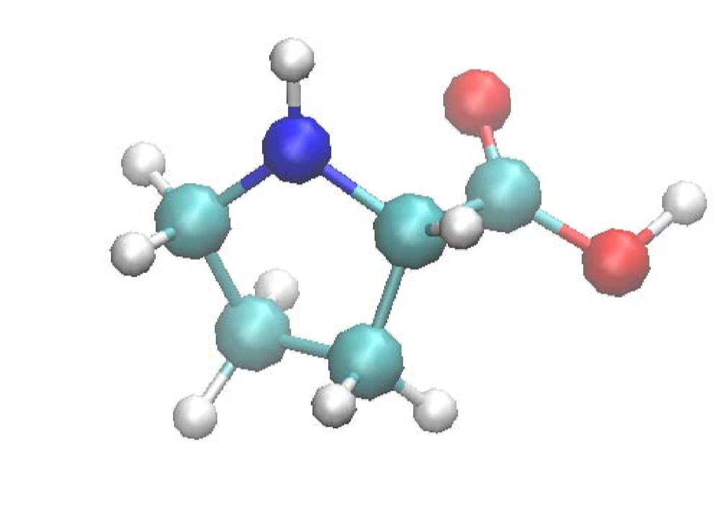
Refer to caption
Refer to caption
Refer to caption
Fig. 3: C5​H9​O2​NC_{5}H_{9}O_{2}N: configuration, charge density and mesh on plane z=0z=0.

The convergence curves of the ground state energy and the a posteriori error estimator ηk​(Ψk,Ω)\eta_{k}(\Psi_{k},\Omega) obtained by the quadratic finite elements are shown in Figure 4, from which we observe that the ground state energy approximations converge to −75.494​a.u.-75.494~a.u., and the a posteriori error estimator decays with a rate −23-\frac{2}{3}. This implies the similar conclusions as those for Example 1.

Refer to caption
(a) ground state energy
Refer to caption
(b) ηh​(Ψh,Ω)\eta_{h}(\Psi_{h},\Omega)
Fig. 4: The convergence curves of the ground state energy and ηh​(Ψh,Ω)\eta_{h}(\Psi_{h},\Omega).

Example 3: Fullerene C60C_{60}.

The ground state energy obtained by SIESTA is −341.340​a.u.-341.340~a.u.. In our computations, we choose Ω=[−30.0,16.0]×[−23.0,22.0]×[−24.0,21.0]\Omega=[-30.0,16.0]\times[-23.0,22.0]\times[-24.0,21.0] to be the computational domain.

We can see the preservation of carbon-hydrogen bonds in Figure 5, which validates our calculations. Figure 5, Figure 6 and Figure 7 show that more mesh points are placed around the atoms.

Refer to caption
Refer to caption
Fig. 5: C60C_{60}: configuration and charge density on a sphere.
Refer to caption
Refer to caption
Fig. 6: C60C_{60}: charge density and mesh on an interior cross-section.
Refer to caption
Refer to caption
Fig. 7: C60C_{60}: charge density and mesh on plane z=0z=0.

The convergence curve of the ground state energy approximations is shown in the right of Figure 8, from which we observe a convergence to −342.722​a.u.-342.722~a.u., which is very close to the reference energy. The convergence curve of the a posteriori error estimator obtained by the quadratic finite element is shown in the left of Figure 8, from which we see that it reaches the optimal convergence rate.

Refer to caption
(a) ground state energy
Refer to caption
(b) ηh​(Ψh,Ω)\eta_{h}(\Psi_{h},\Omega)
Fig. 8: The convergence curves of the ground state energy and ηh​(Ψh,Ω)\eta_{h}(\Psi_{h},\Omega).

6 Concluding remarks

In this paper, we have studied the AFE approximations of Kohn-Sham models. We have obtained the convergence and quasi-optimal complexity of the AFE approximations. We have also curried out some typical numerical simulations that not only support our theory, but also show the robustness and efficiency of the adaptive finite element method in electronic structure calculations.

In our analysis of convergence rate and complexity of AFE approximations, for convenience, we have assumed that the numerical integration was exact and the nonlinear algebraic eigenvalue problem was exactly solved. Indeed, the same conclusion can be expected when the error resulting from the inexact solving of the nonlinear algebraic eigenvalue problem and the error coming from the inexact numerical integration are taken into account.

Suppose that (Λ,Φ)∈Θ(\Lambda,\Phi)\in\Theta, the associated exact solution over mesh 𝒯h\mathcal{T}_{h} is (Λh,Φh)(\Lambda_{h},\Phi_{h}), and the inexact numerical solution is (Λ^h,Φ^h)(\hat{\Lambda}_{h},\hat{\Phi}_{h}). If the numerical errors resulting from the solution of (nonlinear) algebraic system and the numerical integration are small enough, say, satisfy

‖Φh−Φ^h‖1,Ω2+|Λh−Λ^h|≲r~​(h0)​ηh2​(Φ^h,Ω)\displaystyle\|\Phi_{h}-\hat{\Phi}_{h}\|_{1,\Omega}^{2}+|\Lambda_{h}-\hat{\Lambda}_{h}|\lesssim{\tilde{r}}(h_{0})\eta_{h}^{2}(\hat{\Phi}_{h},\Omega)

with r~​(h0)≪1{\tilde{r}}(h_{0})\ll 1 for h0≪1h_{0}\ll 1, then we have from the following triangle inequality

‖Φ−Φ^h‖1,Ω\displaystyle\|\Phi-\hat{\Phi}_{h}\|_{1,\Omega} ≤\displaystyle\leq ‖Φ−Φh‖1,Ω+‖Φh−Φ^h‖1,Ω,\displaystyle\|\Phi-\Phi_{h}\|_{1,\Omega}+\|\Phi_{h}-\hat{\Phi}_{h}\|_{1,\Omega},
|Λ−Λ^h|\displaystyle|\Lambda-\hat{\Lambda}_{h}| ≤\displaystyle\leq |Λ−Λh|+|Λh−Λ^h|,\displaystyle|\Lambda-\Lambda_{h}|+|\Lambda_{h}-\hat{\Lambda}_{h}|,

and the similar perturbation arguments that the same convergence rate and quasi-optimal complexity can be derived.

Finally, we point out that, in this paper, we have not given the convergence rate and complexity for the AFE approximations for the Lagrange multipliers Λ\Lambda. Indeed, the related optimal results for Lagrange multipliers are not so obvious, and we need do some more detailed analysis, which increase the length of this paper. We will report elsewhere.

Appendix: A boundary value problem

In this appendix, we shall provide some basic results for the AFE approximations of a model problem that was used in our previous analysis. Consider a homogeneous boundary value problem:

{ℒ​Φ=Fin​Ω,Φ=0on​∂Ω,\left\{\begin{array}[]{rcll}\mathcal{L}\Phi&=&F&\mbox{in}~~\Omega,\\ \Phi&=&0&\mbox{on}~~\partial\Omega,\end{array}\right. (A.1)

where F=(fi)i=1N∈(L2​(Ω))NF=(f_{i})_{i=1}^{N}\in(L^{2}(\Omega))^{N}. Note that (A.1) is equal to: Find Φ∈ℋ\Phi\in\mathcal{H} such that

a⁡(Φ,Γ)=(F,Γ)∀Γ∈ℋ.\displaystyle a(\Phi,\Gamma)=(F,\Gamma)\hskip 20.00003pt\forall~\Gamma\in\mathcal{H}. (A.2)

A standard finite element scheme for (A.2) is: Find Φh∈Vh\Phi_{h}\in V_{h} satisfying

a⁡(Φh,Γ)=(F,Γ)∀Γ∈Vh.\displaystyle a(\Phi_{h},\Gamma)=(F,\Gamma)\hskip 20.00003pt\forall~\Gamma\in V_{h}. (A.3)

Let 𝕋\mathbb{T} denote the class of all conforming refinements by bisections of 𝒯0\mathcal{T}_{0}. For 𝒯h∈𝕋\mathcal{T}_{h}\in\mathbb{T} and any Γ=(γi)i=1N∈Vh\Gamma=(\gamma_{i})_{i=1}^{N}\in V_{h}, we define the element residual ℛ~τ​(Γ)\tilde{\mathcal{R}}_{\tau}(\Gamma) and the jump J~e​(Γ)\tilde{J}_{e}(\Gamma) by

ℛ~τ​(Γ)\displaystyle\tilde{\mathcal{R}}_{\tau}(\Gamma) =\displaystyle= (fi+12​Δ​γi)i=1Nin​τ∈𝒯h,\displaystyle\left(f_{i}+\frac{1}{2}\Delta\gamma_{i}\right)_{i=1}^{N}\hskip 20.00003pt\mbox{in}~\tau\in\mathcal{T}_{h}, (A.4)
J~e​(Γ)\displaystyle\tilde{J}_{e}(\Gamma) =\displaystyle= (12∇γi|τ1⋅n1→+12∇γi|τ2⋅n2→)i=1None∈ℰh,\displaystyle\left(\frac{1}{2}\nabla\gamma_{i}|_{\tau_{1}}\cdot\overrightarrow{n_{1}}+\frac{1}{2}\nabla\gamma_{i}|_{\tau_{2}}\cdot\overrightarrow{n_{2}}\right)_{i=1}^{N}\hskip 10.00002pt\mbox{on}~e\in\mathcal{E}_{h},

where ee is the common face of elements τ1\tau_{1} and τ2\tau_{2} with unit outward normals n1→\overrightarrow{n_{1}} and n2→\overrightarrow{n_{2}}, respectively. For τ∈𝒯h\tau\in\mathcal{T}_{h}, we define the local error indicator η~h​(Γ,τ)\tilde{\eta}_{h}(\Gamma,\tau) by

η~h2​(Γ,τ)=hτ2​‖ℛ~τ​(Γ)‖0,τ2+∑e∈ℰh,e⊂∂τhe​‖J~e​(Γ)‖0,e2\displaystyle\tilde{\eta}^{2}_{h}(\Gamma,\tau)=h_{\tau}^{2}\|\tilde{\mathcal{R}}_{\tau}(\Gamma)\|_{0,\tau}^{2}+\sum_{e\in\mathcal{E}_{h},e\subset\partial\tau}h_{e}\|\tilde{J}_{e}(\Gamma)\|_{0,e}^{2} (A.5)

and the oscillation osc~h​(Γ,τ)\widetilde{{\rm osc}}_{h}(\Gamma,\tau) by

osc~h​(Γ,τ)=hτ​‖ℛ~τ​(Γ)−ℛ~τ​(Γ)¯‖0,τ.\displaystyle\widetilde{{\rm osc}}_{h}(\Gamma,\tau)=h_{\tau}\|\tilde{\mathcal{R}}_{\tau}(\Gamma)-\overline{\tilde{\mathcal{R}}_{\tau}(\Gamma)}\|_{0,\tau}. (A.6)

Given 𝒯′⊂𝒯h\mathcal{T}^{\prime}\subset\mathcal{T}_{h}, we define the error estimator η~h​(Γ,𝒯′)\tilde{\eta}_{h}(\Gamma,\mathcal{T}^{\prime}) and the oscillation osc~h​(Γ,𝒯′)\widetilde{{\rm osc}}_{h}(\Gamma,\mathcal{T}^{\prime}) by

η~h2​(Γ,𝒯′)=∑τ∈𝒯′η~h2​(Γ,τ)andosc~h2​(Γ,𝒯′)=∑τ∈𝒯′osc~h2​(Γ,τ),\displaystyle\tilde{\eta}^{2}_{h}(\Gamma,\mathcal{T}^{\prime})=\sum_{\tau\in\mathcal{T}^{\prime}}\tilde{\eta}^{2}_{h}(\Gamma,\tau)\hskip 10.00002pt\textnormal{and}\hskip 10.00002pt\widetilde{{\rm osc}}^{2}_{h}(\Gamma,\mathcal{T}^{\prime})=\sum_{\tau\in\mathcal{T}^{\prime}}\widetilde{{\rm osc}}^{2}_{h}(\Gamma,\tau),

respectively. We see that a similar a posteriori error estimate to that for Poisson equation can be expected for (A.1) (c.f. [41, 42, 60]).

Theorem A.19.

Let Φ∈ℋ\Phi\in\mathcal{H} be the solution of (A.2) and Φh∈Vh\Phi_{h}\in V_{h} be the solution of (A.3). Then there exist constants C~1\tilde{C}_{1}, C~2\tilde{C}_{2} and C~3>0\tilde{C}_{3}>0 depending only on cac_{a} in (1) and γ∗\gamma^{\ast} in (15) such that

‖Φ−Φh‖1,Ω2≤C~1​η~h2​(Φh,Ω),\displaystyle\|\Phi-\Phi_{h}\|^{2}_{1,\Omega}\leq\tilde{C}_{1}\tilde{\eta}^{2}_{h}(\Phi_{h},\Omega), (A.7)
C~2​η~h2​(Φh,Ω)≤‖Φ−Φh‖1,Ω2+C~3​osc~h2​(Φh,Ω).\displaystyle\tilde{C}_{2}\tilde{\eta}^{2}_{h}(\Phi_{h},\Omega)\leq\|\Phi-\Phi_{h}\|_{1,\Omega}^{2}+\tilde{C}_{3}\widetilde{{\rm osc}}^{2}_{h}(\Phi_{h},\Omega). (A.8)

An AFE algorithm for (A.2) is designed as follows (c.f. [12]):

Algorithm A.1.
  1. 1.

    Pick a given mesh 𝒯0\mathcal{T}_{0}, and let k=0k=0.

  2. 2.

    Solve (A.3) on 𝒯k\mathcal{T}_{k} to get discrete solution Φk\Phi_{k}.

  3. 3.

    Compute local error indictors η~k​(Φk,τ)\tilde{\eta}_{k}(\Phi_{k},\tau) for all τ∈𝒯k\tau\in\mathcal{T}_{k}.

  4. 4.

    Construct ℳk⊂𝒯k\mathcal{M}_{k}\subset\mathcal{T}_{k} by Dörfler Strategy and parameter θ\theta.

  5. 5.

    Refine 𝒯k\mathcal{T}_{k} to get a new conforming mesh 𝒯k+1\mathcal{T}_{k+1}.

  6. 6.

    Let k=k+1k=k+1 and go to 2.

Using the similar arguments to those for scalar linear elliptic boundary value problem (see, e.g, [12]), we have the following result for Algorithm A.1.

Theorem A.20.

If {Φk}k∈ℕ0\{\Phi_{k}\}_{k\in\mathbb{N}_{0}} is a sequence of finite element solutions produced by Algorithm A.1, then there exist constants γ~>0\tilde{\gamma}>0 and ξ~∈(0,1)\tilde{\xi}\in(0,1) depending only on the shape regularity γ∗\gamma^{\ast} and the marking parameter θ\theta, such that for any two consecutive iterations

‖Φ−Φk+1‖1,Ω2+γ~​η~k+12​(Φk+1,Ω)≤ξ~2​(‖Φ−Φk‖1,Ω2+γ~​η~k2​(Φk,Ω)).\displaystyle\|\Phi-\Phi_{k+1}\|^{2}_{1,\Omega}+\tilde{\gamma}\tilde{\eta}^{2}_{k+1}(\Phi_{k+1},\Omega)~\leq~\tilde{\xi}^{2}\big(\|\Phi-\Phi_{k}\|^{2}_{1,\Omega}+\tilde{\gamma}\tilde{\eta}^{2}_{k}(\Phi_{k},\Omega)\big).

Indeed, the constant γ~{\tilde{\gamma}} has the following form

γ~=1(1+δ−1)​C~∗2\displaystyle\tilde{\gamma}=\frac{1}{(1+\delta^{-1})\tilde{C}^{2}_{\ast}} (A.9)

with C~∗>0\tilde{C}_{\ast}>0 depending on the regularity constant γ∗\gamma^{\ast} and δ∈(0,1)\delta\in(0,1).

For the distance between two nested solutions of (A.3), we have (c.f. [12])

Theorem A.21.

Let ΦH∈VH\Phi_{H}\in V_{H} and Φh∈Vh\Phi_{h}\in V_{h} be solutions of (A.3) respectively. If 𝒯h\mathcal{T}_{h} is a refinement of 𝒯H\mathcal{T}_{H} by marked element ℳH\mathcal{M}_{H} and refined elements ℛ=ℛ𝒯H→𝒯h\mathcal{R}=\mathcal{R}_{\mathcal{T}_{H}\rightarrow\mathcal{T}_{h}}, then

‖ΦH−Φh‖1,Ω2≤C~1​∑τ∈ℛη~H2​(ΦH,τ).\displaystyle\|\Phi_{H}-\Phi_{h}\|^{2}_{1,\Omega}\leq\tilde{C}_{1}\sum_{\tau\in\mathcal{R}}\tilde{\eta}^{2}_{H}(\Phi_{H},\tau).

References

  • [1] R.A. Adams, Sobolev Spaces, Academic Press, New York, 1975.
  • [2] S. Agmon, Lectures on the Exponential Decay of Solutions of Second-Order Elliptic Operators, Princeton University Press, Princeton, 1981.
  • [3] A. Anantharaman and E. Cancès, Existence of minimizers for Kohn-Sham models in quantum chemistry, Ann. I. H. Poincaré-AN, 26 (2009), pp. 2425-2455.
  • [4] I. Babuska and M. Vogelius, Feedback and adaptive finite element solution of one-dimensional boundary value problems, Numer. Math., 44 (1984), pp. 75-102.
  • [5] E. Bänsch and K. Siebert, A Posteriori Error Estimation for Nonlinear Problems by Duality Techniques, Albert-Ludwigs-Univ., Math. Fak., 1995.
  • [6] T.L. Beck, Real-space mesh techniques in density-function theory, Rev. Mod. Phys., 72 (2000), pp. 1041-1080.
  • [7] A.D. Becke, A new inhomogeneity parameter in density-functional theory, J. Phys. Chem., 109 (1998), pp. 2092-2098.
  • [8] R. Becker and R. Rannacher, An optimal control approach to a posteriori error estimation in finite element methods, Acta Numerica, 10 (2001), pp. 1-102.
  • [9] P. Binev, W. Dahmen, and R. DeVore, Adaptive finite element methods with convergence rates, Numer. Math., 97 (2004), pp. 219-268.
  • [10] E.J. Bylaska, M. Holst, and J.H. Weare, Adaptive finite element method for solving the exact Kohn-Sham equation of density functional theory, J. Chem. Theory Comput., 5 (2009), pp 937-948.
  • [11] E. Cancès, R. Chakir, and Y. Maday, Numerical analysis of the planewave discretization of some orbital-free and Kohn-Sham models, M2AN, 46 (2012), pp. 341-388.
  • [12] J.M. Cascon, C. Kreuzer, R.H. Nochetto, and K.G. Siebert, Quasi-optimal convergence rate for an adaptive finite element method, SIAM J. Numer. Anal., 46 (2008), pp. 2524-2550.
  • [13] H. Chen, X. Gong, L. He, Z. Yang, and A. Zhou, Numerical analysis of finite dimensional approximations of Kohn-Sham equations, Adv. Comput. Math., 38 (2013), pp. 225-256.
  • [14] H. Chen, X. Gong, L. He, and A. Zhou, Adaptive finite element approximations for a class of nonlinear eigenvalue problems in quantum physics, Adv., Appl., Math., Mech., 3 (2011), pp. 493-518.
  • [15] H. Chen, L. He, and A. Zhou, Finite element approximations of nonlinear eigenvalue problems in quantum physics, Comput. Methods Appl. Mech. Engrg., 200 (2011), pp. 1846-1865.
  • [16] P.G. Ciarlet, The Finite Element Method for Elliptic Problems, North-Holland, 1978.
  • [17] X. Dai, Adaptive and Localization Based Finite Element Discretizations for the First-Principles Electronic Structure Calculations, Ph.D. Thesis, Academy of Mathematics and Systems Science, Chinese Academy of Sciences, Beijing, 2008.
  • [18] X. Dai, X. Gong, Z. Yang, D, Zhang, and A. Zhou, Finite volume discretizations for eigenvalue problems with applications to electronic structure calculations, Multiscale Model. Simul., 9 (2011), pp. 208-240.
  • [19] X. Dai, L. He, and A. Zhou, Convergence rate and quasi-optimal complexity of adaptive finite element computations for multiple eigenvalues, arXiv:1210.1846, 2012.
  • [20] X, Dai, L. Shen, and A. Zhou, A local computational scheme for higher order finite element eigenvalue approximations, Inter. J. Numer. Anal. Model., 5 (2008), pp. 570-589.
  • [21] X. Dai, J. Xu, and A. Zhou, Convergence and optimal complexity of adaptive finite element eigenvalue computations, Numer. Math., 110 (2008), pp. 313-355.
  • [22] X. Dai and A. Zhou, Three-scale finite element discretizations for quantum eigenvalue problems, SIAM J. Numer. Anal., 46 (2008), pp. 295-324.
  • [23] W. Dörfler, A convergent adaptive algorithm for Poisson’s equation, SIAM J. Numer. Anal., 33 (1996), pp. 1106-1124.
  • [24] R.G. Durán, C. Padra, and R. Rodríguez, A posteriori error estimates for the finite element approximation of eigenvalue problems, Math. Mod. Meth. Appl. Sci., 13 (2003), pp. 1219-1229.
  • [25] A. Edelman, T.A. Arias, and S.T. Smith, The geometry of algorithms with orthogonality constraints, SIAM J. Matrix Anal. appl., 20 (1998), pp. 303-353.
  • [26] J. Fang, X. Gao, and A. Zhou, A Kohn-Sham equation solver based on hexahedral finite elements, J. Comput. Phys., 231 (2012), pp. 3166-3180.
  • [27] J.L. Fattebert, R.D. Hornung, and A.M. Wissink, Finite element approach for density functional theory calculations on locally refined meshes, J. Comput. Phys., 223 (2007), pp. 759-773.
  • [28] S. Fournais, M. Hoffmann-Ostenhof, T. Hoffmann-Ostenhof, and T. ∅\emptyset. S∅\emptysetrensen, Analystic structure of many-body Coulombic wave functions, Comm. Math. Phys., 289 (2009), pp. 291-310.
  • [29] E.M. Garau and P. Morin, Convergence and quasi-optimality of adaptive FEM for Steklov eigenvalue problems, IMA J. Numer. Anal., 31 (2011), pp. 914-946.
  • [30] E.M. Garau, P. Morin, and C. Zuppa, Convergence of adaptive finite element methods for eigenvalue problems, M3AS, 19 (2009), pp. 721-747.
  • [31] S. Giani and I. G. Graham, A convergent adaptive method for elliptic eigenvalue problems, SIAM J. Numer. Anal., 47 (2009), pp. 1067-1091.
  • [32] X. Gong, L. Shen, D. Zhang, and A. Zhou, Finite element approximations for Schrödinger equations with applications to electronic structure computations, J. Comput. Math., 23 (2008), pp. 310-327.
  • [33] L. He and A. Zhou, Convergence and complexity of adaptive finite element methods for elliptic partial differential equations, Inter. J. Numer. Anal. Model., 8 (2011), pp. 615-640.
  • [34] V. Heuveline and R. Rannacher, A posteriori error control for finite element approximations of ellipic eigenvalue problems, Adv. Comput. Math., 15 (2001), pp. 107-138.
  • [35] P. Hohenberg and W. Kohn, Inhomogeneous electron gas, Phys. Rev. B, 136 (1964), pp. 864-871.
  • [36] W. Kohn and L.J. Sham, Self-consistent equations including exchange and correlation effects, Phys. Rev. A, 140 (1965), pp. 1133-1138.
  • [37] M.G. Larson, A posteriori and a priori error analysis for finite element approximations of self-adjoint elliptic eigenvalue problems, SIAM J. Numer. Anal., 38 (2000), pp. 608-625.
  • [38] C. Lee, W. Yang, and R.G. Parr, Development of the Colic-Salvetti correlation-energy formula into a functional of the electron density, Phys. Rev. B, 37 (1988), pp. 785-789.
  • [39] D. Mao, L. Shen, and A. Zhou, Adaptive finite element algorithms for eigenvalue problems based on local averaging type a posteriori error estimates, Adv. Comput. Math., 25 (2006), pp. 135-160.
  • [40] R.M. Martin, Electronic Structure: Basic Theory and Practical Method, Cambridge University Press, Cambridge, 2004.
  • [41] K. Mekchay and R.H. Nochetto, Convergence of adaptive finite element methods for general second order linear elliplic PDEs, SIAM J. Numer. Anal., 43 (2005), pp. 1803-1827.
  • [42] P. Morin, R.H. Nochetto, and K. Siebert, Convergence of adaptive finite element methods, SIAM Review, 44 (2002), pp. 631-658.
  • [43] P. Morin, K.G. Siebert, and A. Veeser, A basic convergence result for conforming adaptive finite elements, Math. Models Methods Appl. Sci., 18 (2008), pp. 707-737.
  • [44] P. Motamarri, M.R. Nowak, K. Leiter, J. Knap, and V. Gavini, Higher-order adaptive finite-element methods for Kohn-Sham density functional theory, J. Comput. Phys., 253 (2013), pp. 308-343.
  • [45] R.G. Parr and W.T. Yang, Density-Functional Theory of Atoms and Molecules, Oxford University Press, New York, Clarendon Press, Oxford, 1994.
  • [46] J.E. Pask, B.M. Klein, P.A. Sterne, and C.Y. Fong, Finite-element methods in electronic-structure theory, Comput. Phys. Commun., 135 (2001), pp. 1-34.
  • [47] J. Pask and P. Sterne, Finite element methods in ab initio electronic structure calculations, Modelling Simul. Mater. Sci. Eng., 13 (2005), pp. R71-R96.
  • [48] J.P. Perdew, K. Burke, and M. Ernzerhof, Generalized gradient approximation made simple, Phys. Rev. Lett., 77 (1996), pp. 3865-3868.
  • [49] M. Reed and B. Simon, Methods of Modern Mathematical Physics, Vol. 2, Academic Press, New York, 1975.
  • [50] R. Schneider, T. Rohwedder, A. Neelov, and J. Blauert, Direct minimization for calculating invariant subspaces in density functional computations of the electronic structure, J. Comput. Math., 27 (2009), pp. 360-387.
  • [51] L. Shen, Parallel Adaptive Finite Element Algorithms for Electronic Structure Computing based on Density Functional Theory, Ph.D. Thesis, Academy of Mathematics and Systems Science, Chinese Academy of Sciences, Beijing, 2005.
  • [52] L. Shen and A. Zhou, A defect correction scheme for finite element eigenvalues with applications to quantum chemistry, SIAM J. Sci. Comput., 28 (2006), pp. 321-338.
  • [53] R. Stevenson, Optimality of a standard adaptive finite element method, Found. Comput. Math., 7 (2007), pp. 245-269.
  • [54] R. Stevenson, The completion of locally refined simplicial partitions created by bisection, Math. Comput., 77 (2008), pp. 227-241.
  • [55] P. Suryanarayana, V. Gavini, T. Blesgen, K. Bhattacharya, and M. Ortiz, Non-periodic finite-element formulation of Kohn-Sham density functional theory, J. Mech. Phys. Solids, 58 (2010), pp. 256-280.
  • [56] T. Torsti, T. Eirola, J. Enkovaara, T. Hakala, P. Havu, V. Havu, T. Hoynalanmaa, J. Ignatius, M. Lyly, I. Makkonen, T.T. Rantala, J. Ruokolainen, K. Ruotsalainen, E. Rasanen, H. Saarikoski, and M.J. Puska,Three real-space discretization techniques in electronic structure calculations, Physica Status Solidi B, 243 (2006), pp. 1016-1053.
  • [57] E. Tsuchida and M. Tsukada, Electronic-structure calculations based on the finite-element method, Phys. Rev. B, 52 (1995), pp. 5573-5578.
  • [58] E. Tsuchida and M. Tsukada, Adaptive finite-element method for electronic-structure calculations, Phys. Rev. B, 54 (1996), pp. 7602-7605.
  • [59] E. Tsuchida and M. Tsukada, Large-scale electronic-structure calculations based on the adaptive finite-element method, J. Phys. Soc. Jpn., 67 (1998), pp. 3844-3858.
  • [60] R. Verfürth, A Review of a Posteriori Error Estimates and Adaptive Mesh-Refinement Techniques, Wiley-Teubner, New York, 1996.
  • [61] Z. Yang, Finite Volume Discretization Based First-Principles Electronic Structure Calculations, Ph.D. Thesis, Academy of Mathematics and Systems Science, Chinese Academy of Sciences, Beijing, 2011.
  • [62] H. Yserentant, Regularity and Approximability of Electronic Wave Functions, Lecture Notes in Mathematics, Springer-Verlag, Berlin, 2010.
  • [63] D. Zhang, Applications of Finite Element Methods in Electronic Structure Calculations, Ph.D. Thesis, Fudan University, 2007.
  • [64] D. Zhang, L. Shen, A. Zhou, and X. Gong, Finite element method for solving Kohn-Sham equations based on self-adaptive terahedral mesh, Phy. Lett. A, 372 (2008), pp. 5071-5076.
  • [65] D. Zhang, A. Zhou, and X. Gong, Parallel mesh refinement of higher order finite elements for electronic structure calculations, Commun. Comput. Phys., 4 (2008), pp. 1086-1105.
  • [66] A. Zhou, An analysis for finite dimensional approximations for the ground state solution of Bose-Einstein condensates, Nonlinearity, 17 (2004), pp. 541-550.
  • [67] A. Zhou, Finite dimensional approximations for the electronic ground state solution of a molecular system, Math. Meth. Appl. Sci., 30 (2007), pp. 429-447.
  • [68] PHG, http://lsec.cc.ac.cn/phg/.