Phase transition and phase coexistence in coupled rings with driven exclusion process
Abstract
We study one-dimensional exclusion processes in two coupled closed rings consisting of a common diffusive channel and two parallel active (driven) channels. Our model displays bulk-driven phase transition and phase coexistence in the form of a localised domain wall (DW) in one of the active channels in a limit where the diffusive and driven dynamics compete. By controlling a splitting parameter which tunes the in-coming currents into the active channels, the system can be brought to a delocalisation transition, when delocalised DWs are formed in both the active channels. We characterise the DW fluctuations numerically.
pacs
64.60.Ht, 05.40.-a, 05.60.-kI Introduction
Totally Asymmetric Simple Exclusion Process (TASEP) [1] serves as a paradigmatic example of open non-equilibrium systems in one dimension (). Its practical realizations include quasi- motion of molecular motors along with microtubules in intra-cellular transport [2], protein synthesis [3] or motion in geometrical confinement, e.g., nuclear pore complex of cells [4]. In contrast, Symmetric Exclusion Process (SEP) [5] is a typical example of diffusion. Well-known examples of SEP include diffusion through artificial crystalline zeolites [6]. In both passive (SEP) and active (TASEP or TASEP-like) systems, prohibition of mutual passage of particles or exclusion gives rise to nontrivial collective effects, whose details of course depend upon whether the dynamics in question is TASEP or SEP. Active systems with open boundaries generally display spatially nontrivial steady state density distributions.
In this paper, we propose a closed model that consists of two overlapping rings with a common diffusive part (SEP) and two parallel active (driven) channels (marked and hereafter). In order to ensure competition between driven and diffusive dynamics, we consider a particular limit of the model. Our principal result includes identification of a model parameter , having values between 0 and 1 (see below), as a switch, by tuning which continuously keeping everything else unchanged (i) one may de-pin pinned domain walls (DW) and (ii) as crosses a localised DW in one of the active channels disappears and appears in the other. Our model should serve as a paradigmatic example of localisation-delocalisation transition in a closed model with coupled diffusive and driven dynamics. In addition to its direct theoretical relevance, it is phenomenologically motivated by the movement of molecular motors in closed compartments [7], the dynamics of colloidal particles in optical traps [8] and the dynamics for multiple mRNAs competing for finite resources (ribosomes), where the ribosomes in turn are bounded by a certain trajectory and a diffusion rate outside the mRNA (during recycling) [9, 10]. In particular, protein synthesis involves two stages: transcription of genetic information from DNA to messenger RNA (mRNA) by RNA polymerase and translation from mRNA to proteins through ribosome translocation. In most bacteria such as E.coli, translation involves three main players: the mRNA (genetic template), the ribosome (assembly machinery), and aminoacyl transfer RNAs (aa-tRNAs), i.e., transfer RNAs “charged” with the corresponding amino acid. The process of translation consists of ribosomes moving along the mRNA without backtracking. This is modeled by TASEP. It is well-known that ribosomes that move along mRNA strand are recycled in a cell. For instance, in eukaryotic cells, after each round of protein synthesis, the ribosomes are released from the mRNA and they join the common pool of ribosomes in cytoplsm, where they execute diffusion and may rejoin the mRNA to restart protein synthesis. In our model, the SEP channel models the “common pool” of diffusive ribosomes in the cytoplasm of an eukaryotic cell, which in our model can come back to the entry point of the TASEP lanes due to the feedback from the SEP channel. However, although ribosome translocation along mRNA forms physical motivation of the present work, the analogy between our model and the actual biological process of ribosome translocation along mRNA strands is not strict due to various limitations of our model, as we discuss below. In both SEP and TASEP, each lattice site has maximum unit occupancy and a particle can only move to the nearest neighbour site (in both directions for SEP or in one direction only for TASEP), only if that site is empty. Thus the dynamics obeys the exclusion principle. For SEP with open boundaries, the density profile is always linear with the slope being determined by the boundary conditions at the two ends [5]. In contrast TASEP with open boundaries displays three distinct phases [11] characterized by their average densities (low and high) and a third phase marked by a maximal current (MC). Unlike with open boundary conditions, individual SEP and TASEP dynamics with closed boundaries (say, closed rings) exhibit only uniform density profile in the steady state due to spatial translational invariance. The rest of the paper is organised as follows: In Sec. II we discuss our model in details. Then in Sec. III we set up our mean-field theory (MFT) and discuss the steady state density profiles by using our MFT, complemented by extensive Monte-Carlo simulation (MCS) studies. In Sec. IV we go beyond MFT, and discuss domain wall fluctuations and delocalisation transition at . Finally, in Sec. V we summarize our results.
II The Model

Our proposed model is a closed system of two overlapping rings consisting of three channels of equal number of sites designated by as shown in Fig. (1). Dynamics of the two channels and are governed by TASEP and the particles in the third channel execute SEP. Thus in particles can hop to both direction with rate , whereas in and particles can only hop to its right neighbour if empty with rate unity setting the time scale. At the left junction of and particles can either enter from SEP channel with rate and respectively if those sites are vacant or can hop to the other side with rate . If both and try to inject a particle into SEP, then one of the TASEP channels ( or ) is selected randomly for injecting a particle to the target site i.e, the first site of SEP if it is empty. If be the total number of particles then, the global particle density In Fig. (1), symbols and refer to the left and right junctions in the model. In addition, for the purpose of clarity, the site number for a particular channel (i.e., , or ) are given as a superscript, e.g., at , the first sites of and are denoted as and , respectively, and the -th site of is denoted as . Similarly for the right junction . In this model, the three bulk parameters control different phase transitions. Thus we observe bulk induced phase transitions unlike the usual TASEP with open boundaries which display boundary induced phase transition. The steady state current in each of SEP, or is a function of and is spatially constant. Notice that our model is a variant and extension of that in Ref. [12]. In particular, for or 0, or is blocked and our model explicitly reduces to that of Ref. [12]. Evidently, for and the behaviour of the two channels are simply interchanged.
III Steady state density profiles
We use mean-field theory (MFT) together with extensive Monte-Carlo simulation (MCS) of our model to obtain the steady state density profiles. In the MFT, the system is considered as a collection of three channels (two TASEP and one SEP) with effective entry and exit rates [13]. Once these effective rates are determined from the condition of constancy of particle currents, one may use them in conjunction with the known results for TASEP and SEP with open boundaries to obtain the density profiles here. Since an isolated TASEP in steady state can be in three different states, the low density (LD), high density (HD) and maximal current (MC) phases, and we have two active (TASEP) channels, there are a number of possibilities for the overall density profile of the two active channels. In order to ensure that the diffusive current does not vanish in the thermodynamic limit (TL, see Ref. [12], see below also) we let diffusivity scales with system size and define a parameter which is the same for any arbitrary system size. Thus steady states of the model are to be parametrised by . Let us now set the notations: for discrete lattice, density at a particular site is defined as , where and refer to and , and for the mean density in the SEP channel . Further in MFT considering continuum limit the density is defined as , where and in TL, lies in the range In all our MFT analysis we use the continuum labelling for the lattice in one dimension. Our main results are summarized in the phase diagrams (parametrised by and ) for and , as shown in Fig. (2), for a representative value of , which are obtained by extensive Monte-Carlo simulations of our lattice-gas model and the corresponding MFT; see below for details. The Monte-Carlo simulations were realized by random sequential update. For any value of (except , when one of the active channels is closed), the phase diagrams of both and may display a combination of the usual LD, HD and MC phases and a region of co-existence of LD and HD phases, i.e., when the density profiles show localised domain walls (DW). The phase co-existence regions are non-overlapping for and , i.e., they do not appear for the same values of and for a given .

At , for which and are statistically symmetric, the density profiles and of and , respectively, are naturally identical. The crucial difference with is that the co-existence region now corresponds to delocalised DWs, i.e., the fraction of the system size visited by a fluctuating DW does not vanish in TL . Such delocalised DWs appear in both and only for . Thus as , the model undergoes a delocalisation transition. The phase diagram for are given in Fig. (3).

To begin with, we denote densities at the junction site by and for the active channels, and and in the passive SEP channel. The SEP current then takes the well-known linear form,
| (1) |
Evidently, remains finite in TL provided scales with linearly, else, for a fixed the SEP current vanishes for . This provides a posteriori justification for the scale-dependent that we have mentioned before. Noting that the current in each of and is given by (assuming no boundary layer at , i.e., are in their LD/coexistence phases) and using conservation of total current at the left and right junctions for the individual incoming/outgoing currents to/from and from/to the SEP channel we obtain
| (2) |
Next, the individual outgoing currents at the sites in and are (again assuming that the channels are in LD or coexistence phase)
| (3) |
Conservation of current then yields As expected, this holds so long as are in their LD or coexistence phase.
In contrast, if are in their HD or coexistence phases the total outgoing current from and to the SEP channel is given by
| (4) |
Conservation of total current at the right junction then yields (assuming to be in HD or coexistence phases)
| (5) |
Further, again assuming HD or coexistence phases for , and separately considering the currents from to yields [14]. This is corroborated by our MCS simulations (see below). This immediately yields that the bulk currents are equal. This is possible only when the bulk currents in are controlled by RJ, i.e., or are both in HD or a combination of coexistence and HD phases. Notice that the conditions obtained for and by using current conservations at the respective sites do not hold simultaneously, unless or are in coexistence phases, such that there are no boundary layers at with being piecewise continuous. Having defined effective entry and exit rates (valid separately for LD/coexistence or HD/coexistence phases in ) for the active channels, we can now apply the known results of TASEP here. One obtains the low (high) density phases in the periodic system equally and are characterized by a uniform density below (above) 1/2 and a boundary layer at the right (left). However for , the boundaries are matched by a piecewise constant density profile with an intervening DW. For TASEP with open boundaries, particle entry and exit events are uncorrelated, and as a result, the DW is delocalised and undergoes random walks covering the entire span of the system in the long time limit. However in the present model, as in Ref. [12], entry and exit of particles are not uncorrelated; they get correlated by the fact that the ends of the active channels are connected by the passive channel. Consequently, as revealed by our Monte Carlo simulation studies, we find localised DW in the active channels, which is similar to Ref. [12]. However, rather surprisingly for the special case of , i.e., when each of the active channels carry equal current on average, we obtain delocalised DWs in both channels. Our MFT formulated above may now be used to analyse the density profiles in the different channels of the model quantitatively.
III.1 DW in one active channel and LD in other
First, let us consider a situation when there is a DW in one of the active channels (say with ) and the other active channel () is in the LD phase with a uniform density (within MFT neglecting any boundary layer). Following the phenomenology of TASEP with open boundaries, we set as a requirement of a DW in . Possibilities of simultaneous DWs in and will be discussed later. Within MFT, may be represented by a Heaviside function that connects the two regions of constant density through a localized DW at position (say) as,
| (6) |
Since is assumed to be in the LD region, density can be written as,
| (7) |
neglecting the boundary layer at the right boundary. For the SEP channel the linear density distribution gives,
| (8) |
Further, the particle number conservation can be expressed as
| (9) |
following the conditions as above and disregarding the discontinuities at the right boundaries. Again from Eq.(2) and Eq.(3) we have,
| (10) |
where Now by solving Eq. (9) in TL () we get
| (11) |
Again Eqs. (4), (5), (10) and the relations and yield for as,
| (12) |
In TL and Since the model considered here is closed, . Again from Eq. (3) we have,
| (13) |
Hence, the position of the DW depends on the two control parameters and for a given . When the DW in is localised within the system (), it connects the LD and HD phases of through a phase of coexistence (LD-HD). The boundaries between the LD, LD-HD phases and LD-HD, HD phases of are obtained by setting and respectively. Setting from Eq.(11) we get a quadratic equation in For a particular value of the feasible values will be Now putting that in Eq. (13) we get the corresponding value. Thus we get the boundary between LD and LD-HD coexistence phase in the -plane. Similar exercise for gives the right boundary between LD-HD and HD phase. See Fig (2) for details. In Fig (2) the phases of channel and are spanned by and . The phase diagrams for and are drawn corresponding to a situation when displays a variety of phases (LD,LD-HD,HD AND MC), while remains in its LD phase. For , this part of the phase diagram remains qualitatively unchanged, with the phase marked as (i.e., in MC and in LD) should expand to a larger area. Similarly, the phases of are shown when channel remains in its HD phase. The condition for the latter is mathematically given by in the bulk. For and hence is no longer in its HD phase. Hence, we do not consider the region while presenting our phase diagram. A DW in obtained from our MCS studies are shown in Fig. (4, top) with , and . We have taken and for determining the position of the domain walls and phase diagram. We do not find any significant dependence of our results on .


III.2 DW in one active channel and HD in other
Let us now consider the case when there is a DW in , and is in HD phase for , thus having a boundary wall at the left end. As discussed above, within MFT, may be represented by Heaviside -function as
| (14) |
and is in HD phase having a uniform density of , neglecting the boundary layer. To have a DW in we must have . Now from Eqs. (4) and (5), we get
| (15) |
Hence Eq. (15) and yield . In TL , and hence, . Again by using the particle number conservation and as and we obtain,
| (16) |
From the above expression we get the boundaries between the LD, LD-HD () and LD-HD, HD phases () of . A DW in , obtained in our MCS studies, is given in Fig. (4, bottom). There is a crucial difference between the DWs in and : The LD part of the DW in has density , different from the density of (fully in LD), thus has no overlap with . In contrast, (fully in HD) overlaps with in the HD part of the DW in . This is due to and is clearly visible in Fig. (4).
III.3 Delocalised domain wall at
Let us now carefully consider the properties for , when both the active channels are symmetric and statistically identical. Thus, if then automatically . Hence, if has a DW, too will have a DW, or is in its LD-HD (co-existence) phase as well, such that its density may be represented by a Heaviside -function that connects the two regions of constant density through a localized DW at (say). Hence, and are given by the expressions (6) and (14) respectively. As both and show DWs, thus and and for from Eq.(2) we have, (say). Again, from Eq.(3) and Eq.(4) we have Therefore, in TL, and thus Now by particle number conservation we have,
| (17) |
Thus for we get a relation given by Eq.(17) between and for a particular value of and In other words and are not uniquely determined. In this case both DWs are delocalized and perform random walk along the active channels. As and are identical, the condition for DW is satisfied for both the channels simultaneously. Thus, and in Eq.(17) can give the boundaries of LD-HD phase in both channels with the LD and HD phases respectively. In Fig. (3) we have shown this mean-field result as well as that obtained from MCS which shows distinct four phases with phase boundaries for both channels are identical. However, symmetry between the two active channels dictate that the long-time
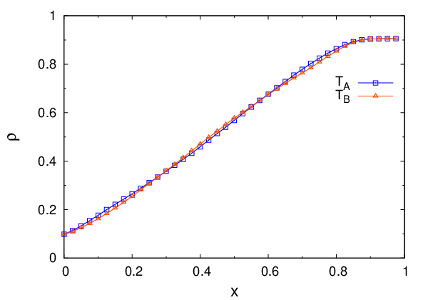
averaged positions of the DWs (equivalently, the long-time average density profiles and ) in and are identical, a fact verified by our MCS, is displayed in Fig. (5).
III.4 Both the active channels in MC phase
Lastly, we consider the possibility of the MC phases in the active channels. Let us first consider the conditions for obtaining MC phases in both the active channels. Condition for MC in isolated TASEPs are and , and this happens when all the boundary densities . Furthermore, have boundary layers at both the ends. This precludes usage of Eq. (3) to determine the boundary densities. Using together with Eq. (2) (assuming no density discontinuities between and ), we find . Since
| (18) |
Using similar considerations at RJ, and again assuming no density discontinuity between and , which means , together with , Eq. 1 and we have,
| (19) |
From particle conservation we have,
| (20) |
Eqs. (18), (19) and (20) yield boundaries of the MC phase with LD and HD phase as, and which indicates the presence of such phase for and bounded by the two above mentioned lines. Thus, the demarcating lines are independent of . They are shown in Fig.(3). We now consider the case when one of the channels (say, ) is in MC phase and the other one () in the LD phase. Therefore, we have , and From Eqn. (2) and (3) we have Again using the MC phase condition we have (arguing as before),
| (21) |
The maximal current condition gives then from particle conservation we have,
| (22) |
The two inequalities (21) together with Eq.(22) then yield boundaries of the MC phase with the LD and HD phase respectively as, and . In Fig. (2) we have shown the MC phase boundaries. Our MCS studies also reveal a small MC phase within the region obtained from MFT. Not surprisingly, for and , the MC phase regions obtained from our MFT match exactly with that of Ref. [12]. In addition, one may argue that the coexistence of in HD and in MC is not possible. For to be in HD phase or . Again , so long as are in HD or coexistence phases. But condition for MC phase in is . Thus, an MC phase in (when in HD) is not allowed.
IV Domain wall fluctuations and delocalisation transition
Until now we have considered the MFT for the model, where all fluctuations are neglected. However, the DWs fluctuate about their MF DW (mean) positions or . We have studied these fluctuations numerically and characterise them by measuring the scaling of the fluctuations with and system size


In particular as from above or below, the localised DW in or shows a delocalisation transition at which DW fluctuations diverge. The width of the distribution of DW fluctuations can be obtained by fitting the density profile in the vicinity of the domain wall by the function [15], with the parameters We find to diverge with a power law dependence on as,
| (23) |
with obtained from our MCS studies as shown in Fig. (6). In contrast, at an off-critical point, i.e., for , DW fluctuations are finite and vanish in TL as ; we have shown this in Fig. (7). For investigating the variation of domain wall width with for various values of we have taken and .
V Summary and outlook
Analytical and numerical studies of our model amply illustrate the underlying rich phase behaviour, including a delocalisation transition, unexpected in a system without boundaries. While boundary-induced phase transitions including delocalisation transitions have been observed in several open systems with exclusion processes together with spatially nontrivial steady state densities [15, 16, 17], analogous studies on bulk closed systems are less studied so far. The competition between the diffusive and driven dynamics, and the division of the SEP current into two parallel TASEP currents are crucial to the macroscopic behaviour we obtained. The latter is controlled by a parameter , which is a tuning parameter in the model. The most striking feature in our work vis-a-vis the results in Ref. [12] is the possible existence of a delocalisation transition and correspondingly the formation of DWs in both and simultaneously at a special value . In contrast to the DWs formed either in or (but not simultaneously in both) for , as found in Ref. [12] as well as in the present work, the DWs at are no longer pinned to a fixed point in the lattice with vanishing fluctuations in the thermodynamic limit. Instead they delocalise and have position fluctuations that do not vanish in the thermodynamic limit. Thus the parameter in our model appears as a tuning parameter or a switch, which can be used to control the nature of domain wall fluctuations (localised/delocalised). In addition for the value of can be tuned to make the DW appear or disappear in one of the active channels. There is no analogue of these in the study of Ref. [12]. While we have considered only two TASEP channels, many more may be added and studied systematically as above. Recalling protein synthesis by ribosomes along mRNA strands as one of the phenomenological motivation for our model, it may be noted that several mRNAs compete for same resources (ribosomes) in a cell. Thus a systematic study of multiple TASEP channels connected in parallel with a single SEP channel would be useful. The failure of the traditional MFT calls for further analysis by means of more sophisticated analytical techniques, e.g., Bethe ansatz [17] or density matrix renormalisation group [18], which are beyond the scope of the present work. From the point of view of nonequilibrium statistical mechanics, our model belongs to the class of models lacking translation invariance and without boundaries that displays a phase transition (in the form of a delocalisation transition). Our model may be extended in several new directions, e.g., again motivating by ribosome movements along mRNA, one may in our model consider particle exchanges between and , or between one of the active channels and passive channel (representing ribosome attachments or detachments), allow defects along the active channels (representing defects in the mRNA), introduce a second control parameter at the exit ends of and that controls the relative outgoing currents to SEP and unequal hopping rates in and . These will be considered elsewhere. We close this work with a note of caution: As mentioned in the beginning, despite some similarities our model cannot be directly used for quantitative descriptions of ribosome translocations along mRNA strands due to its limiations. First of all, ribosome diffusion takes place inside a cell, which, alothough geometrically confined, has a three-dimensional () structure, as opposed to our diffusive model for it. Secondly, the description of a ribosome as a single unit (i.e., a point particle here) is also questionable, for it gets released from an mRNA by falling apart into different subunits, a feature not possible to capture in our simplified description here. Nevertheless, our work provides some clues about the actual biological system, e.g., the crucial role of particle number conservation in determining the nature of the steady states. We expect that more realistic theoretical descriptions of ribosome translocation and detachment should have some of the basic features of our model in-built into it.
Acknowledgements.
AB wishes to thank the Max-Planck-Gesellschaft (Germany) and Department of Science and Technology (India) for partial financial support through the Partner Group programme (2009). AKC acknowledges the financial support from DST (India) under the SERC Fast Track Scheme for Young Scientists [Sanction no. SR/FTP/PS-090/2010(G)].References
- [1] B. Schmittmann and R. Zia, in Phase Transitions and Critical Phenomena, edited by C. Domb and J. Lebowitz (Academic Press, London, 1995); T. Chou, K. Mallick and R. K. P. Zia, Rep. Prog. Phys. 74, 116601 (2011).
- [2] J. Howard, Mechanics of Motor Proteins and the Cytoskeleton (Sinauer Associates, Sunderland, 2001).
- [3] J. T. MacDonald, J. H. Gibbs, and J. H. Pipkin, Biopolymers 6, 1 (1968); T. Chou, Biophys. J. 85, 755 (2003); Alberts B, Johnson A, Lewis J, et al, Molecular Biology of the Cell, Garland Science, New York (2002).
- [4] I. Kosztin and K. Schulten, Phys. Rev. Lett. 93 (2004).
- [5] G. Schšutz, in Phase Transitions and Critical Phenomena, edited by C. Domb and J. Lebowitz (Academic Press, London, 2000).
- [6] J. Kärger and D. Ruthven, Diffusion in zeolites and other micropourous solids (Wiley, New York, 1992).
- [7] R. Lipowsky, S. Klumpp, and T. M. Nieuwenhuizen, Phys. Rev. Lett. 87, 108101 (2001).
- [8] Q.-H. Wei, C. Bechinger, and P. Leiderer, Science 287, 625 (2000).
- [9] L. J. Cook, R. K. P. Zia and B. Scmittmann, Phys. Rev. E 80 031142 (2009).
- [10] R. K. P. Zia, J. J. Dong, and B. Schmittmann, Journal of Statistical Physics 144, 405 (2011).
- [11] J. Krug, Phys. Rev. Lett. 67, 1882 (1991).
- [12] H. Hinsch and E. Frey, Phys. Rev. Lett. 97, 095701, (2006); Jiang et al, Phys. Rev. Lett. 106, 079601 (2011); Hinsch et al Phys. Rev. Lett. 106, 079602 (2011).
- [13] See J. Brankov, N. Pesheva and N. Bunzarova, Phys. Rev. E, 69, 066128 (2004).
- [14] Obtaining the same result by using the particle-hole symmetry, that a single TASEP admits in a straightforward way, is tricky here; see, e.g., B. Embley et al, Phys. Rev. E 80, 041128 (2012) for extensive discussions on this.
- [15] T. Reichenbach, T. Franosch and E. Frey, Eur. Phys. J. E, 27, 47 (2008).
- [16] A. Parmeggiani, T. Franosch and E. Frey, Phys. Rev. Lett. 90, 086601 (2003).
- [17] G. Schülz, in Phase Transitions and Critical Phenomena, edited by C. Domb and J. Lebowitz (Academic Press, London, 2000).
- [18] U. Schollwöck, Rev. Mod. Phys. 77, 259 (2005).