Strings attached: New light on an old problem Thanks: The first author was supported in part by NSF grant DMS-1206272.
Abstract.
The wave equation is generally regarded as a linear approximation to the equation describing the amplitude of a transversely vibrating elastic string in the plane. But, as is shown in [2], the assumption of transverse vibration in fact implies that the wave equation describes the vibration precisely, with no need for approximation. We give a simplified proof of this result, and we generalize to the case of an elastic string vibrating (transversely or not) in a Riemannian surface . In the more general setting, the assumption of transverse vibration is replaced by the assumption of “perfect elasticity,” and we show that the wave map equation gives a precise description of the vibration of a perfectly elastic string in , with no need for approximation. Finally, we give examples describing the motion of various vibrating strings in , , and .
1. Introduction
One of the most familiar partial differential equations in all of mathematics is the wave equation for a vibrating string,
| (1.1) |
which describes the transverse vibration of an elastic string the in the plane. The equilibrium position of the string is assumed to be an interval along the -axis, and the function represents the vertical displacement at time of the point on the string corresponding to the point with equilibrium position .
A wide variety of methods have been used to derive equation (1.1) from physical principles; we will critically review some of the best-known derivations ([7], [6], [12]) in §2. The methods discussed here vary in the specific techniques used during the derivation process, but they all make use of simplifying assumptions and/or approximations (e.g., constant tension, small amplitude vibrations), with the result that equation (1.1) is deemed to be only a linear approximation to the “true” wave equation. Exceptions to this approach in the literature are rare; a few can be found in [1], [2], [8], [16].
In §3, we will start from scratch and carry out a derivation of the wave equation from physical principles, without any of the simplifying assumptions made in most derivations. Our derivation is along the lines of that given in [2], but it is more straightforward. Remarkably, it turns out that all the nonlinearities cancel each other out, and equation (1.1) is the correct equation for the motion of a transversely vibrating elastic string—not “just” a linear approximation. In light of the simplicity of our derivation, we find it remarkable that this fact is not better known than it appears to be, and that the presumed “nonlinear string equation” has persisted for many decades in textbooks.
In §4, we will consider generalizations of equation (1.1) to the case of an elastic string with not-necessarily-transverse vibration, both in the Euclidean plane and in an arbitrary Riemannian surface , where the notion of “transverse” vibration is not well-defined in general. In this more general setting, the assumption of transverse vibration is replaced by the assumption of “perfect elasticity” (cf. Definition 3.1). We will see that with this assumption, the motion is governed by the wave map equation
| (1.2) |
for the function , where represents the Levi-Civita connection of the Riemannian metric on . (We refer the reader to [13], [11], and [14] for information on wave maps.) Again, while the wave map is often portrayed as a “first approximation” (see, e.g., [13]) to the motion of an elastic string, we will show that in fact no simplifying assumptions are needed in order to derive the wave map equation (1.2) from the physical principles governing the motion of the string. In §5 we give some examples of solutions to (1.2) in non-flat Riemannian surfaces. Note that here the partial differential equation governing the motion of the string on a non-flat Riemannian surface is intrinsically nonlinear. This arises from the non-Euclidean nature of the ambient space in which the vibrations are taking place.
2. Many derivations, many assumptions
Consider an elastic string of constant linear density , whose equilibrium position lies along the interval in the -axis. Suppose that the string is allowed to vibrate only in the transverse direction, so that at time , the position in the -plane of the point on the string corresponding to the point with equilibrium position is given by .
2.1. The Courant-Hilbert derivation
In Courant and Hilbert’s classic text [7], the wave equation is derived from Lagrangian mechanics and the calculus of variations. Simplifying assumptions include:
- •
The magnitude of the tension in the string is assumed to be constant.
- •
The vibrations are assumed to have “small” amplitude, so that the quantity can be approximated by its first-order Taylor polynomial .
The kinetic energy of the string is given by
while the potential energy is assumed to be proportional to the increase in the string’s length compared to its length at rest; i.e.,
This leads to the Lagrangian functional
whose Euler-Lagrange equation is
Setting yields the wave equation (1.1).
2.2. The Coulson-Jeffrey derivation
Coulson and Jeffrey’s well-known text [6] takes a different approach that avoids the calculus of variations, and instead considers the forces acting on a small segment of the string, corresponding to the interval . Simplifying assumptions include:
- •
The magnitude of the tension in the string is assumed to be constant.
- •
While it is noted that the condition for to be approximately constant is that “the wave disturbance is not too large,” this assumption is not made explicit as in the Courant-Hilbert derivation until fairly late in the process.
The equation of motion for this segment of the string is given by Newton’s law of motion ; as the vibration is assumed to be transverse, only the vertical component of the motion is considered.
For each fixed , let denote the angle between the tangent vector to the string at the point and the horizontal, as shown in Figure 2.1.
The vertical component of the force exerted on the right-hand end of the string segment is given by , while the vertical component of the force exerted on the left-hand end of the string segment is given by , so that the total vertical force acting on the string segment is
The arc length of the string segment is approximately
and so the mass of the string segment is assumed to be
Note that this assumption is incorrect: the mass of this string segment at rest is equal to , not , and conservation of mass implies that the mass remains equal to regardless of how the string is stretched. (This error appears frequently—although not universally—in the literature; it is generally inadvertently remedied at a later stage in the derivation where is assumed to be small, and therefore .) Since , Newton’s equation becomes:
Dividing by and taking the limit as yields
| (2.1) | ||||
The trigonometric identities
| (2.2) |
imply that
Therefore,
| (2.3) |
and equation (2.1) is equivalent to the nonlinear equation
| (2.4) |
(If the mass of the string segment had been correctly represented as instead of , equation (2.4) would instead have become
| (2.5) |
Only at this stage in the derivation do Coulson and Jeffrey apply the assumption that is small, so that equation (2.4) may be approximated by the linearized form (1.1), with .
2.3. The undergraduate version
Yet another variant on this derivation appears in many undergraduate PDE textbooks; as an example, we present a slight variation on the derivation given in [12]. In this version, assumptions about the tension and the magnitude of are postponed until later in the process. As in the Coulson-Jeffrey derivation, this argument is based on Newton’s equation applied to the string segment corresponding to the interval , but this time Newton’s equation appears in its vector form . With the same notation as in §2.2 (and using , the vertical component of Newton’s equation becomes
| (2.6) |
while the horizontal component becomes (due to the assumption of transversality)
| (2.7) |
First consider equation (2.7). Dividing by and taking the limit as yields
Now the simplifying assumption is made that is “small,” and therefore
hence, . So is now assumed to be approximately constant, but in this case the assumption of constant tension is a consequence of the hypothesis of transverse motion and the assumption that the vibrations are “small,” rather than a separate assumption.
3. A more accurate derivation
In this section we present an alternative derivation for equation (1.1). We will follow the general strategy of the derivation of §2.3, but we will assume only that the vibration is transverse, so that motion occurs only in the vertical direction. No a priori assumptions will be made about either the function (except that it is assumed to be differentiable) or the magnitude of the vibrations. (Derivations using only these assumptions are given in [2] and [8]; ours is similar, but more straightforward.)
As in §2.3, we apply Newton’s equation to the string segment corresponding to the interval , which leads to equations (2.6) and (2.7). Dividing both of these equations by and taking the limit as yields the equations
| (3.1) | |||
| (3.2) |
First consider equation (3.2). Write this equation as
and substitute in the trigonometric identities (2.2), (2.3) to obtain
| (3.3) |
Equation (3.3) may be regarded as a separable differential differential equation for the function : rewrite equation (3.3) as
Now integrate and exponentiate to obtain:
| (3.4) |
where is an arbitrary function of .
Observe that, for each fixed , equation (3.4) says that the magnitude of the tension of the string at the point is proportional to the derivative of the arc length function
with respect to the curve parameter . Assuming that the physical parameters of the string are not changing in time, it is reasonable to assume that the “constant” of proportionality is, in fact, equal to a constant , which represents the tension of the string in its equilibrium position. The quantity
may be regarded as the “stretching factor” of the string at the point , and, following [16], we make the following definition:
Definition 3.1.
A string is called perfectly elastic provided that, when the string at tension is stretched by a factor of , the tension becomes equal to .
Thus, equation (3.4) may be interpreted as saying that the hypothesis of transverse vibrations implies that the string is perfectly elastic, merely as a consequence of Newton’s law. This observation is significant enough that we state it as:
Proposition 3.2.
The tension of an elastic string vibrating transversely in the plane must satisfy the perfect elasticity condition (3.4).
Remark 3.3.
Perfect elasticity is a special—and idealized—case of the more familiar notion of “linear elasticity.” Linear elasticity refers to a string that satisfies Hooke’s Law, which in its infinitesimal version says that, at a point where the string’s stretch factor is equal to , the tension in the string is proportional to , where is the value of for which the tension is equal to zero. Perfect elasticity is the special case where , which mathematically corresponds to a string which shrinks to a point in the absence of external forces. As a practical matter, this condition is almost certainly never precisely satisfied by real physical strings; however, a rubber band or a spring stretched to several times its natural length may satisfy it to a reasonable approximation. (Physical data supporting this assertion may be found in [8].) Consequently, the vibrating motion of real physical springs can never be truly transverse, but only approximately so.
4. Vibrating strings in Riemannian surfaces
Now consider the problem of an elastic string of constant linear density vibrating in a Riemannian surface . Even the innocuous-sounding assumption of “constant linear density” merits some examination. If a string is represented by a parametrized curve
for some interval , then the density of the string is represented by a 1-form on , defined by the condition that the mass of any segment of the string is given by
“Constant linear density” is generally taken to mean that for some constant , but in fact this condition is dependent on the parametrization of the string. A string with any smooth, nonvanishing density -form can always be given a reparametrizion with the property that for some constant . (In fact, by taking to be the function
we can arrange that ; however, it is often convenient to allow other values of , so we will allow to be any positive constant.)
Definition 4.1.
Let be a connected interval, and let be a local coordinate on . A parametrized curve in a Riemannian surface with a specified density 1-form on is said to be parametrized by constant density if for some constant .
As observed above, a string with any smooth, nonvanishing density 1-form can be parametrized by density, so the assumption of “constant linear density” must mean something more than simply having the string parametrized by constant density. In the classical case of a string vibrating transversely in the plane, the condition of constant linear density is characterized by the fact that the equilibrium position of the string has a parametrization which is simultaneously a parametrization by constant density and a parametrization by arc length. As the vibrating string expands and contracts, however, the parametrization for the position of the string at a given time generally does not remain an arc length parametrization for the curve—but it does remain a constant density parametrization.
Next, consider the notion of “transverse vibrations.” In the classical case of the string vibrating in the plane, “transverse” is taken to mean “in the vertical direction.” This notion relies crucially on the canonical local coordinates on the plane, and on the vertical vector field defined on any open neighborhood in the plane. But for a general Riemannian surface, there are no canonical local coordinates, and hence there is no obvious way to define the notion of a “transverse” vibration. (Even if we attempted to accomplish this by defining a “transverse” vector field orthogonal to a curve representing the equilibrium position of some particular string, there is still no canonical way to extend such a vector field to an open neighborhood of the given curve segment.)
Therefore, in light of Proposition 3.2 we replace the assumption of “transverse vibration” with an assumption of perfect elasticity, which does make sense even in the more general setting of a Riemannian surface. But this too requires some care: according to Definition 3.1, a string is perfectly elastic if the tension in the string is directly proportional to the stretch factor . But like the constant linear density condition, this condition is dependent on the parametrization of the string. Since Definition 3.1 was formulated under the assumption of a constant density parametrization for the string, we now make the following refinement in order to make this assumption explicit:
Definition 4.2.
A string in a Riemannian surface with a constant density parametrization is called perfectly elastic for in the range provided that, when the string at tension is stretched by a factor of , the tension becomes equal to .
In order to derive the equation of motion for the general case of a string vibrating in a Riemannian surface , we will assume that:
- •
the string is parametrized by constant density;
- •
the string is perfectly elastic;
- •
the motion of the string is governed by Newton’s Law.
Corollary 4.4 will show that these conditions suffice to guarantee that a constant density parametrization for a string in equilibrium position is also a constant speed parametrization with respect to an arc length parameter along the curve segment. This is the natural analog to the “constant linear density” assumption in the classical case; the fact that it follows from the assumption of perfect elasticity suggests that perhaps the notion of perfect elasticity is more subtle than it might appear.
We are now ready to state our main result:
Theorem 4.3.
Let be a Riemannian surface with Levi-Civita connection , and let be a smooth map, where for each fixed , the curve represents the position of a string vibrating in at time . Suppose that the string is parametrized by constant density and perfectly elastic, and that its motion is governed by Newton’s Law. Then the map satisfies the wave map equation
| (4.1) |
Corollary 4.4.
The equilibrium position of a string in a Riemannian surface satisfying the conditions of Theorem 4.3 consists of a segment of a geodesic curve in . Furthermore, the given constant density parametrization of this curve segment is also a constant-speed parametrization with respect to an arc length parameter along the curve segment.
Proof of Corollary 4.4. Any equilibrium solution is independent of ; therefore . Then (4.1) implies that the solution curve satisfies the geodesic equation
which implies that is a constant-speed geodesic segment in . ∎
For the sake of clarity, we will prove Theorem 4.3 in two steps: first we give a proof in the case that is the flat plane , where we can take advantage of the canonical identification between tangent planes at each point of . Then we will indicate how the proof may be generalized for an arbitrary Riemannian surface .
Proof of Theorem 4.3. First suppose that , and let
For fixed , consider the string segment corresponding to the interval and the (vector-valued) tension forces acting at the endpoints of the string segment. (See Figure 4.1.)
According to the assumption of perfect elasticity, the magnitude of the force vector is equal to
for some positive constant ; similarly, the magnitude of the force vector is equal to
The direction of is given by the unit tangent vector
to the curve at the point , while the direction of at the point is given by
Therefore, we have
Thus the total force acting on the string segment is
| (4.2) |
Since is assumed to be a constant density parametrization, the mass of the string segment is given by . Now Newton’s equation becomes
| (4.3) |
Dividing by and taking the limit as yields
Taking yields
which is equivalent to (4.1) for the standard flat connection on .
For a general Riemannian surface , we must make the following modifications to this proof:
- •
In Newton’s equation, the acceleration vector must be replaced by .
- •
The expression
in (4.2) no longer makes sense because the tangent vectors , are based at different points of . In order to remedy this, we must replace the vector by its parallel transport backwards along the curve from to .
Substituting these changes into equation (4.3), dividing by and taking the limit as yields the wave map equation (4.1).
∎
5. Examples
In this section we compute several examples of solutions to equation (4.1) (with ) in various Riemannian surfaces. These examples illustrate how solutions may be affected not only by the geometry of the surface , but also by the choice of a density 1-form along the string. (The choice of is implicit in the choice of parametrization for the initial data curve, as this curve is assumed to be parametrized by constant density.)
For each example we will specify a Riemannian surface and an initial curve segment in . We will give an explicit representation for the PDE system (4.1) in terms of local coordinates on , and we will numerically solve this system for the given initial data, assuming fixed endpoints and zero initial velocity.11 1 All numerical solutions were computed in Maple 16 using the “pdsolve/numeric” function with standard options.
Example 5.1.
Let be the flat plane. With local coordinates and the standard flat metric on , the wave map equation (4.1) is equivalent to the system
| (5.1) |
for the functions .
Suppose that the initial curve is the graph of for . The classical case of “constant linear density” along this curve is represented by the parametrization
This parametrization leads to the classic solution
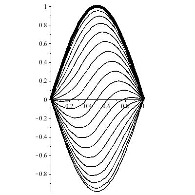
Some curves in this evolution are shown in Figure 5.1; the initial curve is drawn as a thick curve, while subsequent curves in the evolution are thinner.

Now suppose that instead of the density 1-form , we choose , so that the density of the string is an affine linear function of the initial -coordinate of the string. This corresponds to choosing , which yields the parametrization
for the initial data curve. The system (5.1) can be solved explicitly, either by Fourier series or by D’Alembert’s formula; some curves in this evolution are shown in Figure 5.2.
Note that, regardless of the initial curve, the general theory of the linear wave equation guarantees that the fixed-endpoint problem will have periodic solutions. The period, however, depends on the parametrization: if the initial curve has parametrization
then the vibration of the string will have period equal to .
Example 5.2.
Let be the unit sphere in , with local parametrization
The standard metric on is given by
and the wave map equation on is equivalent to the system
| (5.2) | ||||
This is a nonlinear system, and its solutions are not periodic in general.
By analogy with our previous example, we will consider “sinusoidal” initial curves. First suppose that the initial curve is described in local coordinates on by the equation
with parametrization
Figure 5.3 shows the evolution of the curve through three cycles in the vibration; as in the last example, the thick curve in each picture represents the initial curve for that portion of the evolution. Note that this solution is only quasi-periodic, as the shape of the wave changes with each successive cycle.


The effect of the nonlinearity becomes more significant if we increase the amplitude of the initial curve: suppose that the initial curve is described in local coordinates on by the equation
with parametrization
Figure 5.4 shows the evolution of the curve through three cycles in the vibration; note that the shape of the wave varies dramatically and even becomes non-embedded at times.


Example 5.3.
Let be the Poincaré upper half plane
with its standard metric
The wave map equation on is equivalent to the system
| (5.3) | ||||
As in the previous example, this is a nonlinear system, and its solutions are not periodic in general.
We will consider several different initial curves. First consider the horizontal line segment for , with parametrization
(Recall that this curve is not a geodesic in .) Figure 5.5 shows the evolution of the curve through three cycles in the vibration; the solution appears almost (but not quite) periodic.


Next, consider a “sinusoidal” perturbation of a vertical geodesic segment. In order that the initial curve appear approximately sinusoidal with respect to the Poincaré metric, we will take the curve
as our initial curve, so that the horizontal line segment from the point to the point has length . (Note that this is still only approximately sinusoidal, since the horizontal line segment joining these two points is not a geodesic.) Furthermore, we will parametrize this curve according to an arc length parametrization for the corresponding vertical line segment along the -axis:
Figure 5.6 shows the evolution of the curve through three cycles in the vibration; one intriguing feature of this evolution is that within each cycle, the string moves to the left much more rapidly than to the right.


As in the previous example, the effect of the nonlinearity becomes more significant if we increase the amplitude of the initial curve: suppose that the initial curve is described by the equation
with parametrization
Figure 5.7 shows the evolution of the curve through three cycles in the vibration; now the shape of the wave varies dramatically and even becomes non-embedded at times.


6. Conclusion
In this paper we have shown that the classical, frictionless, elastic string under tension undergoing transverse vibrations in the Euclidean plane is exactly modeled by the linear wave equation,
| (6.1) |
regardless of the size of the vibrations, and that this PDE is not a small amplitude approximation of a “nonlinear string equation.” More generally, if the arena of the vibration changes from the Euclidean plane to an arbitrary Riemannian surface, such the 2-sphere or the Poincare half-plane , then the motion of the string is governed by the partial differential equation for wave maps into Riemannian surfaces:
| (6.2) |
The wave map equation is intrinsically nonlinear whenever the Gauss curvature of the target space of the wave map is non-zero. Equation (6.1) is essentially the wave map equation for wave maps into the Euclidean plane. Equation (6.2) is a source of fascination for both the mathematician and physicist. If forces cease to act on the string, then the left hand side of (6.2) will vanish, and the resulting differential equation will be that of a geodesic of the Riemannian surface. Hence (6.2) generalizes the notion of geodesics and provides a very interesting class of hyperbolic partial differential equations for geometric analysis ([11], [14]). For the mathematician, there are still many basic questions that remain open. On the other hand, the same partial differential equation arises, for instance, in elementary particle physics ([9]) and general relativity ([10], [4], [3]).
One natural question to consider is which Riemannian surfaces give rise to wave maps with particularly nice properties. In [5] we have begun an exploration of wave maps for which the corresponding wave map system is Darboux integrable; we plan to delve more deeply into this topic in future work. Another area which we hope to explore in the near future is that of sub-Riemannian geometry; the context in which we have discussed wave maps here as parametrized curves evolving in time still makes sense in sub-Riemannian geometry, and questions such as global existence of solutions and integrability are of interest.
References
- [1] Stuart S. Antman, The equations for large vibrations of strings, Amer. Math. Monthly 87 (1980), no. 5, 359–370.
- [2] David Bleecker and George Csordas, Basic Partial Differential Equations, International Press, Cambridge, MA, 1996.
- [3] Yvonne Choquet-Bruhat, Global wave maps on curved space times, Mathematical and quantum aspects of relativity and cosmology (Pythagoreon, 1998), Lecture Notes in Phys., vol. 537, Springer, Berlin, 2000, pp. 1–29.
- [4] by same author, Global wave maps on black holes, Jean Leray ’99 Conference Proceedings, Math. Phys. Stud., vol. 24, Kluwer Acad. Publ., Dordrecht, 2003, pp. 469–482.
- [5] Jeanne N. Clelland and Peter J. Vassiliou, A solvable string on a lorentzian surface, arXiv:1303.0087 [mathAP (math.DG)], Mar., 2013.
- [6] C. A. Coulson and Alan Jeffrey, Waves: A mathematical account of the common types of wave motion, second ed., Longman, Inc., New York, N.Y., 1977.
- [7] R. Courant and D. Hilbert, Methods of mathematical physics. Vol. I, Interscience Publishers, Inc., New York, N.Y., 1953.
- [8] Joseph B. Keller, Large amplitude motion of a string, Amer. J. Phys. 27 (1959), 584–586.
- [9] Sergei V. Ketov, Quantum non-linear sigma-models, Texts and Monographs in Physics, Springer-Verlag, Berlin, 2000, From quantum field theory to supersymmetry, conformal field theory, black holes and strings.
- [10] Charles W. Misner, Harmonic maps as models for physical theories, Phys. Rev. D (3) 18 (1978), no. 12, 4510–4524.
- [11] Jalal Shatah and Michael Struwe, Geometric wave equations, Courant Lecture Notes in Mathematics, vol. 2, New York University Courant Institute of Mathematical Sciences, New York, 1998.
- [12] Walter Strauss, Partial differential equations: An introduction, John Wiley and Sons, Inc., 1992.
- [13] Terence Tao, Wave maps, http://www.math.ucla.edu/tao/preprints/wavemaps.pdf.
- [14] Chuu-Lian Terng and Karen Uhlenbeck, wave maps into symmetric spaces, Comm. Anal. Geom. 12 (2004), no. 1-2, 345–388.
- [15] Peter J. Vassiliou, Cauchy problem for a Darboux integrable wave map system and equations of Lie type, SIGMA Symmetry Integrability Geom. Methods Appl. 9 (2013), 024, 21 pp.
- [16] Darryl Yong, Strings, chains, and ropes, SIAM Rev. 48 (2006), no. 4, 771–781 (electronic).