UNAVOIDABLE CMB SPECTRAL FEATURES AND BLACKBODY PHOTOSPHERE OF OUR UNIVERSE
Abstract
Spectral features in the CMB energy spectrum contain a wealth of information about the physical processes in the early Universe, . The CMB spectral distortions are complementary to all other probes of cosmology. In fact, most of the information contained in the CMB spectrum is inaccessible by any other means. This review outlines the main physics behind the spectral features in the CMB throughout the history of the Universe, concentrating on the distortions which are inevitable and must be present at a level observable by the next generation of proposed CMB experiments. The spectral distortions considered here include spectral features from cosmological recombination, resonant scattering of CMB by metals during reionization which allows us to measure their abundances, -type distortions during and after reionization and -type and -type (intermediate between and ) distortions created at redshifts .
keywords
CMB,Cosmology,Origin and formation of the Universe,Background radiations,Observational cosmology,Intergalactic matterPACS
PACS numbers:98.80.-k,98.80.Bp,98.70.Vc,98.80.Es,98.62.Ra1 Spectral distortions of CMB
The remarkable measurement of the cosmic microwave background spectrum (CMB) by COBE/FIRAS [1] showed that the CMB is almost a perfect blackbody with temperature and was not able to detect any distortions from a blackbody. However, the standard model of cosmology predicts distortions in the spectrum from processes which heat, cool, scatter and create CMB photons, throughout most of the history of the Universe. Many of these processes are connected with absolutely new physics. The goal of the present paper is not to list all possible sources of distortions from physics beyond the standard model but to point out the unavoidable distortions predicted in the standard model. These distortions are small but fortunately significant progress in technology in the last two decades permits an improvement of 2–3 orders of magnitude over COBE/FIRAS [2]. New proposals like Pixie [3], CoRE [4] and LiteBIRD [5] promise to detect the majority of the unavoidable spectral distortions we discuss in this paper. Pixie will be able to make absolute measurements as well as measure anisotropies with an angular resolution of . CoRE and LiteBIRD will be able to measure only the frequency dependent anisotropies with high sensitivity and have proposed angular resolutions of and respectively. The detection of these spectral distortions would provide new information about the important properties of the Universe such as reionization and formation of the first stars and galaxies at redshifts , recombination of hydrogen and helium at redshifts and energy injection at redshifts due to the dissipation of sound waves in the primordial plasma. We will also discuss the effect of rapidly cooling baryons and electrons leading, under some additional conditions, to Bose-Einstein condensation of CMB photons.
2 Line features from the epoch of hydrogen and helium recombination
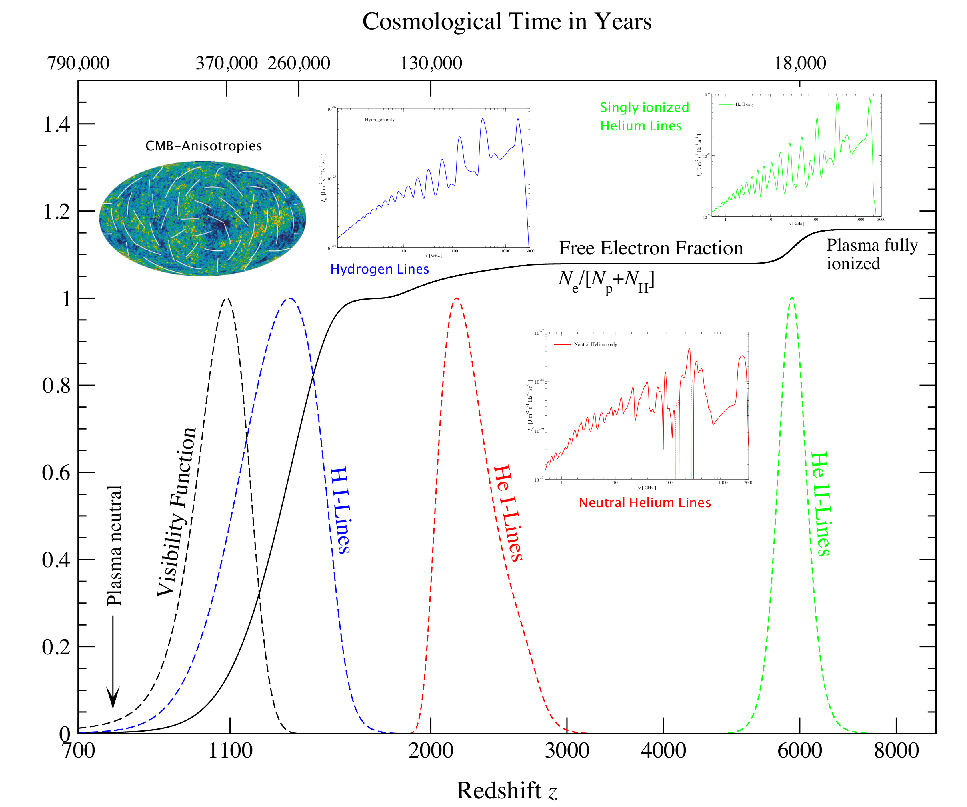


One of the most important phase transitions in the history of the Universe is recombination of electrons with protons and helium nuclei to form neutral atoms [12, 13]. The standing sound waves, excited by primordial initial perturbations, in the previously tightly coupled electron-baryon-photon plasma are frozen into the free streaming photons [6, 14] and are observed today by CMB experiments such as COBE/DMR [15], BOOMERANG [16], ACBAR [17], WMAP [18], SPT [19], ACT [20] and many others.11 1 A more complete list of CMB experiments is available on NASA LAMBDA website, http://lambda.gsfc.nasa.gov/product/expt The recombination of HeIII to HeII at redshift , HeII to HeI at and HII to HI at is accompanied by the release of recombination radiation from electrons cascading down to the ground states of recombining atoms. The recombination radiation from Ly- and 2-photon transitions was first mentioned by Kurt, Zeldovich and Sunyaev [12] and Peebles [13] while Dubrovich [21] pointed out the importance of transitions in the hydrogen atoms for the observations of the recombination spectrum. The full recombination spectrum was calculated in Refs [10, 22, 11]. Fig. 1 shows the line profiles for the recombination lines. It is interesting to note that for hydrogen most of the recombination photons are emitted significantly earlier than the last scattering surface (where the Thomson visibility function is peaked). Fig. 2 shows the hydrogen recombination spectrum and Fig. 3 demonstrates the contributions from helium to the total recombination spectrum. The x-axes shows the observed frequency today which is redshifted by a factor of from the rest frame frequencies and appear today in the radio part of the electromagnetic spectrum. Lyman, Balmer and higher series lines are easily identifiable. Approximately photons per hydrogen atom are emitted. Presence of helium adds additional spectral features in the recombination spectrum in Fig. 3; these features would provide a completely independent measure of the primordial helium abundance if the cosmological recombination lines will be detected. Proposed experiment PIXIE [3] would have the sensitivity to detect the CMB recombination spectrum at [23].
3 Frequency dependent blurring of the CMB anisotropies from resonant scattering by metals and a way to measure the abundance of metals during the epoch of reionization
Planck mission [24] will provide us with sensitive independent measurements of the cosmic microwave background (CMB) angular fluctuations in different spectral bands. Using just the existing Planck channels, we can find upper limits (and possibly a measurement) of the abundance of several important ions, such as OIII, OI, CII, NII etc, at different redshifts. The sensitivity to the presence of metals between the last scattering surface (LSS) and us comes from the resonant scattering of the primordial angular fluctuations of CMB by atoms and ions in the intergalactic space between halos and regions inside halos with density smaller than the critical density, when collisions are unimportant [25]. This resonant line scattering by atoms and ions, just like Thomson scattering from electrons, blurs the CMB anisotropies on scales smaller than horizon,
| (1) |
where is the observed temperature anisotropy in CMB today in the direction , is the anisotropy we would see if the optical depth to the last scattering surface was zero, i.e. there was no reionization. Formally, this solution arises as the boundary term in the line of sight integral solution of the first order Boltzmann equation of photons [26, 27]. The total optical depth has a frequency independent part arising from Thomson scattering[28], and a frequency dependent part arising from the scattering with metals, . was calculated for almost all the important metal species in Ref. [25]. Figure 4

from Ref [25] shows the total optical depth as well as the contributions from individual metal species for two different models of ionization and metal production. The effect of the non-zero optical depth to the LSS is to blur the anisotropies, i.e. the hot spots become colder and the cold spots become warmer. The angular power spectrum is suppressed by a factor of . The best signal-to-noise in the power spectrum is, of course, obtainable for the anisotropies around the first acoustic peak of CMB, around angular wavenumber . We can of course use all the CMB fluctuation data below the horizon size at the redshift of scattering, and up to the angular resolution limit of Planck , to improve the sensitivity. Alternatively, we can stack up all the hot and cold spots in the cleanest portions of the sky and measure the difference in their temperatures at different frequencies, . This analysis would be similar to the one done by the WMAP team to detect polarization generated at the last scattering surface [28]. They found hot spots and cold spots with rms temperature fluctuation of K. In our case, the resonant scattering of the radiation will decrease the spot brightness of hot spots at the frequency of observation, , if there is significant amount of the corresponding ion at redshift , where is the rest frame frequency of the resonant line. Similarly, resonant scattering will decrease the amplitude of the cold spots, increasing their brightness. Fig. 4 shows that resonant scattering is unable to blur the fluctuations at low frequencies, because they correspond to high redshifts () where there are negligible amount of metals, for the lines of most abundant ions. By comparing the brightness of hot and cold spots at different frequencies, we have an opportunity to measure the abundance of ions during the epoch of reionization. The analysis is limited not by sensitivity but by the calibration error. A detection of an optical depth of using the hottest and coldest spots with temperature fluctuation K would require a calibration accuracy of K. Any difference between two frequency channels above the calibration error would be due to resonant scattering and will constrain the presence of metals between us and the last scattering surface. Possible limits are shown in Fig. 5 for the most important metal species.

The limits on the metal abundance obtained in this way from the blurring effect are density averaged limits. Sensitivity of Planck in the HFI channels is respectively at using just of sky for 14 months of operation [24] and much better when using all the data and averaging over all modes. Planck thus has, in principle, opportunity to get independent upper limits to the difference in optical depth to LSS seen by different frequency channels, if the frequency channels can be calibrated relatively to each other precisely. The most promising method of calibration is by using the orbital dipole of the Planck spacecraft. The motion of the earth and Planck satellite in the solar system can be measured with exquisite precision. In fact, for the WMAP satellite, the orbital dipole is known at a precision of nK [29] and it is thus, in principle, possible to achieve a calibration precision at the level of for the hottest/coldest spots with temperature fluctuation of K, improving the numbers presented in Fig. 5 by a factor of 100! An additional precise source of calibration with well defined spectrum is also provided by the -type distortion quadrupole induced by our motion with respect to the CMB[30, 31, 32].
4 -type spectral distortions
The primordial plasma of our Universe is of very low density. Average number density of photons exceeds that of the electrons by a factor of . Under these circumstances, Compton scattering of radiation on free thermal electrons (taking into account the Doppler shift of photon energy, the recoil effect and double Compton scattering) is the most important physical process responsible for the interaction of matter and radiation in the Universe. Our Universe is optically thin to bremsstrahlung absorption and emission of CMB photons[33] almost up to the time of positron-electron annihilation which occurred at redshifts .


The interaction of CMB blackbody photons (temperature ) with the plasma (temperature ) is described by the Kompaneets equation [36]. The Kompaneets equation is the Fokker-Planck approximation of Boltzmann equation with Compton scattering,
| (2) |
where we have defined
| (3) |
is the dimensionless frequency, is the Planck’s constant, is frequency, is the Boltzmann’s constant. Also, is the Hubble parameter, is the electron number density and is the maximum redshift at which we start the calculation. The three terms in the right-hand side brackets in Eq. (2) describe the change in photon frequency due to recoil (), induced recoil and Doppler effect () respectively. The (induced) recoil and Doppler effects cancel each other if the photon spectrum is a Planck/Bose-Einstein spectrum with temperature and , making the right-hand side vanish.
The -type distortion is the solution of the Kompaneets equation in the minimal comptonization limit, . This solution, in the small distortion limit, is easily obtained by approximating the occupation number on the right hand side of Eq. (2) by Planck spectrum (), and using . The resulting differential equation is now trivial to integrate, giving ( for )[33]
| (4) |
where the amplitude of the distortion is proportional to the electron pressure (in the limit ), integrated along the line of sight,
| (5) | ||||
| (6) |
For constant temperature , is proportional to the integrated Thomson optical depth, . If the total energy injected into the CMB is , where is the energy density of the CMB, then the -type distortion is given by [33] . Eq. (5) also shows that we have a positive distortion for and a negative distortion for . -type distortion is shown in Figs. 6 and 7
4.1 -type distortions from reionization and WHIM

Present observations indicate that the Universe was reionized between redshifts of [28], when the first stars and galaxies flooded the Universe with ultraviolet radiation. The ionizing radiation also heated the gas to temperatures well above the CMB temperature, with the electron temperature in the ionizing regions . Late time structure formation shock heated the gas to even higher temperatures [38], , creating the warm-hot intergalactic medium (WHIM)[39]. The optical depth, , to the last scattering surface is well constrained by CMB observations [28] to be , assuming CDM cosmology. Thus if , we expect . However if a significant fraction of baryons end up in the WHIM at , as expected from recent simulations [39, 40], we expect the -distortions from the WHIM to dominate over those from reionization [41]. In any case, these distortions would be easily detected by PIXIE [3] and the next generation CMB experiments like CoRE [4], ACTPol [42] and SPTPol [43] should also be able to detect the fluctuations in the -type distortions from the the WHIM. The rate of -type distortion injection with redshift is shown in Fig. 8 for a simple model where reionization happens between and the density averaged temperature of free electrons is assumed to be for and at [39]. The contribution from the WHIM to the -type distortions dominates over those from reionization in this model.
4.2 -type distortion from averaging of blackbodies in our CMB sky


The temperature of the CMB in the sky is not constant but is a function of direction. The most significant anisotropy comes from our peculiar motion with respect to the CMB rest frame (i.e the frame in which the CMB dipole is zero). Our peculiar velocity, or equivalently the CMB dipole seen in our rest frame, was measured very precisely by COBE [1] and WMAP [45] experiments and has an amplitude . In addition, there are small scale anisotropies of amplitude in the microwave sky due to the presence of primordial density perturbations. If we average the CMB intensity over all angles or part of the sky, either explicitly to improve the sensitivity or because of the finite beam of the telescope, we will inevitably mix the blackbodies of different temperatures. It was shown in Ref. [46] that mixing of blackbodies gives rise, at the lowest non vanishing order, to a -type distortion and that the thermal -type distortion from comptonization is just superposition of blackbodies. This result is quite general and is also applicable if the source of electron motion is not thermal but kinetic, i.e. there is a -type distortion arising from peculiar motion of baryons. As a simple example, superposition of two blackbodies with temperatures is shown in Fig. 9 (intensity) and Fig. 10 (effective temperature). The resulting spectrum after averaging can be recognized as a blackbody with higher temperature with a -type distortion of amplitude [47, 44]. For the dipole anisotropy in our sky, we get and averaging of the rest of the smaller scale anisotropies (without dipole) contribute . The -type spectrum provides, in principle, a high precision source to calibrate CMB experiments [31].
5 -type distortions
The thermal capacity of electrons and baryons is negligible in comparison with that of photons and Compton interaction rapidly establishes a Maxwellian distribution of electrons with temperature defined by the radiation (photon) field [48, 49]. If the spectrum of photons is Bose-Einstein spectrum then the equilibrium electron temperature is exactly equal to the radiation temperature. The other way around, the timescale for the establishment of equilibrium Bose-Einstein spectrum for photons through Compton scattering is comparatively much longer compared to the age of the Universe at redshifts , see Fig. 11 and the discussion below.

Bose-Einstein spectrum with chemical potential parameter 22 2 Our definition of is equivalent to the negative of the usual statistical physics chemical potential divided by temperature, making it dimensionless and we will call it chemical potential parameter. and temperature , is the equilibrium solution of the Kompaneets equation, as can be readily verified by substituting it in Eq. (2). The reference temperature now corresponds to a blackbody spectrum with the same number density of photons as the Bose-Einstein spectrum, and the factor is there because we have defined the dimensionless frequency with reference to . For small distortions, , we can expand the Bose-Einstein spectrum around the reference blackbody giving, for the -type distortion (using[50] ),
| (7) |
The intensities of and -type distortions are plotted in Fig. 7. The parameter is related to the fractional energy injected into the CMB by[51, 50] .
The -type distortion is thus the solution of the Kompaneets equation in the saturated comptonization limit, for . The function is plotted in Fig. 11. If , comptonization is very efficient in establishing a Bose-Einstein spectrum if energy is injected at redshift , while for only a -type distortion can be created from the heating or cooling of the CMB. We should note that, on the contrary, the -parameter in Eq. (5) describes the amplitude of injected energy/-type distortion and is always much smaller than unity for the physical processes considered in this paper.
5.1 Negative and distortions from Bose-Einstein condensation of CMB


It was recognized long ago [12] that in the early Universe, when baryons and photons are tightly coupled, the photons must transfer energy to the baryons to keep them in equilibrium (until ), as baryons cool adiabatically faster () than radiation () with the expansion of the Universe. This is simply because the baryons are non-relativistic with an adiabatic index of compared to the adiabatic index of for the relativistic photon gas. This (small) cooling of the CMB gives rise to spectral distortions ( and intermediate-type) which are exactly the negative of the distortions caused by the heating of the CMB. Figure 12 shows the -type distortion resulting from the cooling of the CMB. The -type distortion resulting from the cooling of the CMB is shown in Fig. 13 along with a positive distortion resulting from an equivalent amount of heating. There is, however, one very important physical difference between the heating and the cooling of the CMB. The cooling of the CMB results in an excess in the number density of photons compared to the blackbody radiation with the same energy density, and this can be recognized as the condition for the Bose-Einstein condensation of photons to happen [50, 44]. In the case of the CMB, of course, the condensing photons, moving to lower frequencies due to the stimulated scattering and the recoil effect, are efficiently destroyed by bremsstrahlung and double Compton absorption [37, 44], and no actual photon condensate[52] is formed.
6 Beyond and : Intermediate-type distortions

The -type distortions are created at redshifts , when the comptonization is minimal. At , the Compton parameter and we get -type distortion, which is the solution of the Kompaneets equation, Eq. (2) in the saturated comptonization limit. The energy injected between the redshifts is only partially comptonized as the Compton parameter is , see Fig 11. The spectrum created from the energy injection in this redshift range is therefore in between -type distortion (minimal comptonization) and a -type distortion (saturated comptonization). Figure 14 shows the spectrum that would be obtained if the energy is injected at redshifts corresponding to different parameters. In practice, the energy is more likely to be injected continuously over a redshift range rather than instantaneously at a single redshift and we expect the observed spectrum to be a linear superposition (with appropriate weights) of the distortions for different values of . Since the intermediate-type spectrum depends on the redshift of energy injection, there is additional information here compared to the and -type distortions which only remember the total energy injected and not the exact time of energy injection. The rather simple behavior of the intermediate-type distortions with respect to the energy injection redshift opens up the possibility to measure the redshift dependence of the energy injection rate. For example, in case of Silk damping or dark matter annihilation we the energy injection rate is a power law in redshift, and with the intermediate-type distortion we can measure the parameter and thus the spectral index of the primordial power spectrum. Combining the intermediate-type distortions and the -type distortions also allows to distinguish between a power law energy injection and the exponential dependence of energy injection rate on the redshift expected from particle decay. Intermediate-type distortions are explored in detail in Ref. [35].
7 Blackbody photosphere of the Universe

The blackbody spectrum of CMB is created dynamically in the early Universe, initially because of the complete thermal equilibrium between the photons and the electrons/positrons (and other particles at even higher redshifts) through pair creation and annihilation and bremsstrahlung. Subsequent adiabatic expansion of the Universe preserves the blackbody spectrum, except small BEC effects described in section 5.1 above. Once pair production becomes inefficient at , double Compton scattering () and bremsstrahlung () become the dominant mechanism of photon absorption and emission at low frequencies while Compton scattering () efficiently redistributes the photons in energy (comptonization). The redistribution of energy among the available photons by comptonization establishes a Bose-Einstein spectrum with a chemical potential parameter at while the emission/absorption of photons by double Compton and bremsstrahlung drives the chemical potential parameter to zero at creating a Planck spectrum.
Understanding the creation of the blackbody spectrum therefore requires solving the Kompaneets equation [36], describing comptonization, with the source terms arising from bremsstrahlung and double Compton scattering [59, 60]. A quite accurate solution to this partial differential equation for comptonization with a source term responsible for the emission and absorption of photons was found analytically in Ref. [51]. Although Ref. [51] only considered bremsstrahlung as the emission/absorption mechanism, the double Compton scattering cross section is similar enough to bremsstrahlung that their method of solution could be applied immediately to the double Compton

scattering also. This was done in Ref. [62] for a low baryon density Universe such as ours, where double Compton scattering dominates over bremsstrahlung. Recently, corrections to this solution were computed in Ref. [63] and a solution with an accuracy of including both bremsstrahlung and double Compton processes was presented. The solution describes the evolution of the chemical potential parameter of the Bose-Einstein spectrum created at redshift and is given by
| (8) |
where, defines the blackbody surface, behind which is exponentially suppressed. The Bose-Einstein spectrum with the effect of this exponential suppression of chemical potential at low frequencies is shown in Fig. 16. The precise analytic solution for the blackbody visibility function derived in Ref. [63] , including the effects of bremsstrahlung and double Compton, is plotted in Fig. 15, curve ’d’. Thus any perturbations away from the Planck spectrum are suppressed exponentially at . The electron-positron annihilation at more than doubles the entropy and energy in photons, but the deviations resulting from the Planck spectrum never rise above a tiny value of [63]. This demonstrates how difficult, almost impossible, it is to create deviation from the Planck spectrum at , in the blackbody photosphere.
8 Energy release in the early Universe
8.1 Spectral distortions from Silk damping: A view of inflation spanning 17 e-folds!
Primordial adiabatic perturbations excite standing sound waves on entering the horizon in the early Universe in the tightly coupled electron-baryon-photon fluid [64, 6, 14].

On small scales, there is shear viscosity and thermal conductivity in the fluid which dissipates the energy in the sound waves, suppressing the fluctuations [67, 14, 68]. Microscopically, photon diffusion through the plasma creates a local quadrupole, which is dissipated by shear viscosity, and relative motion between the photons and the baryons creates a local dipole, which is dissipated by thermal conduction or Compton drag. This Silk damping of primordial fluctuations is already observed by the current

CMB experiments SPT[19] and ACT[20] with high precision. The power which disappears from the fluctuations appears in the average CMB spectrum or monopole as , and intermediate-type spectral distortion [69, 70, 71, 37, 44, 47, 72, 73]. In Fig. 15, The heating rate of CMB from sound wave dissipation is compared with the cooling due to the energy transfer to baryons for several different power spectra allowed by the current CMB data [28]. It is interesting to note that the cases where cooling dominates over heating for -type distortions are still allowed if there is non-zero running of the spectral index, although for most of the region of the parameter space heating dominates over cooling. These distortions can be added together linearly since they are very small. The -type and the intermediate-type spectral distortions are created by the dissipation of modes with comoving wavenumbers . Most of this range of scales is inaccessible to any other cosmological probe. When combined with the information from the CMB anisotropies and the large scale structure, this gives us a view of inflation spanning e-folds compared with e-folds () without the spectral distortions, as depicted in Fig. 17. The CMB spectral distortions are thus measuring the primordial power spectrum on extremely small scales and are very important to our understanding of the physics of the initial conditions. Possible constraints from PIXIE are shown in Fig. 18. Recently, precise calculations of these distortions were done in Ref. [47] including previously ignored effects such as second order Doppler effect and fitting formulae for and -type parameters were also provided. Distortions for several other non-standard and general initial conditions were calculated in Refs. [74, 75] and the effect of non-Gaussian initial conditions on correlations was pointed out in Refs. [76, 77].
8.2 A census of unavoidable and -type distortions in standard cosmology
A census of unavoidable and -type distortions in standard cosmology is given in Tables 1 and 2. Public codes KYPRIX[78] and CosmoTherm[37] are now available to calculate the evolution of CMB spectral distortion by numerically solving the Kompaneets equation with bremsstrahlung and double Compton terms, starting in the blackbody photosphere at . Many of the processes shown in Tables 1 and 2 were first calculated in Ref. [37]. The CosmoTherm code also includes high precision calculations of Silk damping and other important cases of energy injection. A fast and precise Mathematica code to calculate the spectral distortions for user-defined energy injection rates, taking advantage of the analytic solution described above and pre-computed numerical templates described in the next section, is also publicly available33 3 http://www.mpa-garching.mpg.de/~khatri/idistort.html.
We stress here again the importance of blackbody photosphere, see Fig. 15. The CMB spectrum does not carry any information about even strong energy injection deep inside the blackbody photosphere. Any injected energy behind the blackbody surface, , is almost completely thermalized without any observable traces in the CMB spectrum. The best example of the strength of equilibrium restoring processes (Compton and double Compton scattering, bremsstrahlung) at high redshifts is the huge energy release, , from electron positron annihilation. The resulting deviations from the complete equilibrium (blackbody, ) even in this extreme case are just !.
| Process | |
|---|---|
| electron-positron annihilation | |
| BBN tritium decay | |
| BBN decay | |
| WIMP dark matter annihilation | |
| Silk damping | |
| Adiabatic cooling of matter and | |
| Bose-Einstein condensation |
| Process | |
|---|---|
| WIMP dark matter annihilation | |
| Silk damping | |
| Adiabatic cooling of matter and | |
| Bose-Einstein condensation | |
| Reionization/WHIM | |
| Mixing of blackbodies: CMB multipoles |
8.3 Constraining new fundamental physics with spectral distortions
Most of the talk has been concentrated on the spectral distortions expected in standard cosmology. The physics beyond the standard model provides numerous new possible sources of heating for CMB. In particular, it is clear from Tables 1 and 2 that in standard cosmology we expect and intermediate-type distortions with an amplitude of . A distortion of larger magnitude, if detected, would thus undoubtedly be a signal of new physics. In addition, the most important standard source of energy injection, Silk damping, has a power law dependence on redshift, resulting in almost an equal amount of energy in -type and intermediate-type distortions [35]. Thus if one of the -type or the intermediate type distortion is stronger than the other, it would again signify new physics. Some of the possible sources of energy injection from new physics are dark matter decay and annihilation [79, 80, 81], decay of cosmic strings and other topological defects, cosmic string wakes and oscillating superconducting cosmic strings [82, 83, 84], photon-axion inter-conversion [85, 86], violation of reciprocity relation [87], dissipation of primordial magnetic fields [88], quantum wave function collapse [89], and evaporating primordial black holes [90].
9 The future looks good for CMB spectroscopy
Three proposed next generation CMB experiments PIXIE [3], COrE [4] and LiteBIRD [5] would have the sensitivity to detect most of the spectral features considered in this review. Current specifications of PIXIE, in particular, with 400 frequency channels and absolute calibration, are optimal to detect the global , and intermediate-type distortions. COrE and LiteBIRD would have the sensitivity and the angular resolution to detect metals during the epoch of reionization and angular fluctuations in the -type sky from the warm-hot intergalactic medium. In the near future, therefore, we expect many interesting results from the observations of the spectral features in the CMB.
References
- [1] D. J. Fixsen, E. S. Cheng, J. M. Gales, J. C. Mather, R. A. Shafer and E. L. Wright, ApJ 473 (1996) 576.
- [2] D. J. Fixsen and J. C. Mather, ApJ 581 (2002) 817.
- [3] A. Kogut, D. J. Fixsen, D. T. Chuss, J. Dotson, E. Dwek, M. Halpern, G. F. Hinshaw, S. M. Meyer, S. H. Moseley, M. D. Seiffert, D. N. Spergel and E. J. Wollack, JCAP 7 (2011) 25.
- [4] The COrE Collaboration, ArXiv e-prints (2011) arXiv:1102.2181 [astro-ph.CO].
- [5] M. Hazumi et al., LiteBIRD: a small satellite for the study of B-mode polarization and inflation from cosmic background radiation detection Society of Photo-Optical Instrumentation Engineers (SPIE) Conference Series 8442 (September 2012), p. 844219.
- [6] R. A. Sunyaev and Y. B. Zeldovich, ApSS 7 (1970) 3.
- [7] B. J. T. Jones and R. F. G. Wyse, A&A 149 (1985) 144.
- [8] G. Hinshaw et al., ApJS 148 (2003) 135.
- [9] R. A. Sunyaev and J. Chluba, Astronomische Nachrichten 330 (2009) 657.
- [10] J. Chluba and R. A. Sunyaev, A&A 458 (2006) L29.
- [11] J. A. Rubiño-Martín, J. Chluba and R. A. Sunyaev, A&A 485 (2008) 377.
- [12] Y. B. Zeldovich, V. G. Kurt and R. A. Sunyaev, Zh. Eksp. Teor. Fiz. 55 (1968) 278.
- [13] P. J. E. Peebles, ApJ 153 (1968) 1.
- [14] P. J. E. Peebles and J. T. Yu, ApJ 162 (1970) 815.
- [15] E. L. Wright, C. L. Bennett, K. Gorski, G. Hinshaw and G. F. Smoot, ApJL 464 (1996) L21.
- [16] W. C. Jones et al., ApJ 647 (2006) 823.
- [17] C. L. Reichardt et al., ApJ 694 (2009) 1200.
- [18] D. Larson et al., ApJS 192 (2011) 16.
- [19] R. Keisler et al., ApJ 743 (2011) 28.
- [20] R. Hlozek et al., ApJ 749 (2012) 90.
- [21] V. K. Dubrovich, Soviet Astronomy Letters 1 (1975) 196.
- [22] J. A. Rubiño-Martín, J. Chluba and R. A. Sunyaev, MNRAS 371 (2006) 1939.
- [23] A. Kogut, private communication (2011).
- [24] Planck Collaboration, Planck blue book (2005).
- [25] K. Basu, C. Hernández-Monteagudo and R. A. Sunyaev, A&A 416 (2004) 447.
- [26] U. Seljak and M. Zaldarriaga, ApJ 469 (1996) 437.
- [27] S. Dodelson, Modern cosmology (Modern cosmology / Scott Dodelson. Amsterdam (Netherlands): Academic Press. ISBN 0-12-219141-2, 2003).
- [28] E. Komatsu et al., ApJS 192 (2011) 18.
- [29] G. Hinshaw et al., ApJS 148 (2003) 63.
- [30] M. Kamionkowski and L. Knox, Phys.Rev.D 67 (2003) 063001, astro-ph/0210165.
- [31] J. Chluba and R. A. Sunyaev, A&A 424 (2004) 389.
- [32] R. A. Sunyaev and R. Khatri, JCAP 3 (March 2013) 12, arXiv:1302.6571 [astro-ph.CO].
- [33] Y. B. Zeldovich and R. A. Sunyaev, ApSS 4 (1969) 301.
- [34] R. A. Sunyaev and Y. B. Zeldovich, Comments on Astrophysics and Space Physics 4 (1972) 173.
- [35] R. Khatri and R. A. Sunyaev, JCAP 9 (2012) 16.
- [36] A. S. Kompaneets, Zh. Eksp. Teor. Fiz. 31 (1956) 876.
- [37] J. Chluba and R. A. Sunyaev, MNRAS 419 (2012) 1294.
- [38] R. A. Sunyaev and Y. B. Zeldovich, A&A 20 (August 1972) 189.
- [39] R. Cen and J. P. Ostriker, ApJ 514 (1999) 1.
- [40] R. Cen and J. P. Ostriker, ApJ 650 (2006) 560.
- [41] B. B. Nath and J. Silk, MNRAS 327 (2001) L5.
- [42] M. D. Niemack et al., ACTPol: a polarization-sensitive receiver for the Atacama Cosmology Telescope Society of Photo-Optical Instrumentation Engineers (SPIE) Conference Series 7741 (2010), p. 77411.
- [43] J. J. McMahon et al., SPTpol: an instrument for CMB polarization, in American Institute of Physics Conference Series, eds. B. Young, B. Cabrera and A. Miller, American Institute of Physics Conference Series, Vol. 1185 (2009), pp. 511–514.
- [44] R. Khatri, R. A. Sunyaev and J. Chluba, A&A 540 (2012) A124.
- [45] N. Jarosik et al., ApJS 192 (2011) 14.
- [46] Y. B. Zeldovich, A. F. Illarionov and R. A. Sunyaev, Soviet Journal of Experimental and Theoretical Physics 35 (1972) 643.
- [47] J. Chluba, R. Khatri and R. A. Sunyaev, MNRAS 425 (2012) 1129.
- [48] Y. B. Zeldovich and E. V. Levich, Soviet Journal of Experimental and Theoretical Physics Letters 11 (1970) 35.
- [49] E. V. Levich and R. A. Sunyaev, Soviet Astronomy 15 (1971) 363.
- [50] A. F. Illarionov and R. A. Sunyaev, Soviet Astronomy 18 (1975) 413.
- [51] R. A. Sunyaev and Y. B. Zeldovich, ApSS 7 (1970) 20.
- [52] J. Klaers, J. Schmitt, F. Vewinger and M. Weitz, Nature 468 (2010) 545.
- [53] S. Dodelson and M. S. Turner, Phys.Rev.D 46 (October 1992) 3372.
- [54] B. D. Fields, S. Dodelson and M. S. Turner, Phys.Rev.D 47 (May 1993) 4309, arXiv:astro-ph/9210007.
- [55] A. D. Dolgov, Physics Reports 370 (November 2002) 333, arXiv:hep-ph/0202122.
- [56] G. Mangano, G. Miele, S. Pastor, T. Pinto, O. Pisanti and P. D. Serpico, Nuclear Physics B 729 (2005) 221.
- [57] L. Kawano, Let’s Go: Early Universe. Guide to Primordial Nucleosynthesis Programming, http://www-thphys.physics.ox.ac.uk/people/SubirSarkar/bbn.html, (1988).
- [58] R. V. Wagoner, ApJ 179 (January 1973) 343.
- [59] A. P. Lightman, ApJ 244 (1981) 392.
- [60] K. S. Thorne, MNRAS 194 (1981) 439.
- [61] R. A. Sunyaev and Y. B. Zeldovich, Comments on Astrophysics and Space Physics 2 (March 1970) 66.
- [62] L. Danese and G. de Zotti, A&A 107 (1982) 39.
- [63] R. Khatri and R. A. Sunyaev, JCAP 6 (2012) 38.
- [64] E. M. Lifshitz, J. Phys. (USSR) 10 (1946) 116.
- [65] P. McDonald, U. Seljak, S. Burles, D. J. Schlegel, D. H. Weinberg, R. Cen, D. Shih, J. Schaye, D. P. Schneider, N. A. Bahcall, J. W. Briggs, J. Brinkmann, R. J. Brunner, M. Fukugita, J. E. Gunn, Ž. Ivezić, S. Kent, R. H. Lupton and D. E. Vanden Berk, ApJS 163 (2006) 80.
- [66] U. Seljak, A. Slosar and P. McDonald, JCAP 10 (2006) 14.
- [67] J. Silk, ApJ 151 (1968) 459.
- [68] N. Kaiser, MNRAS 202 (1983) 1169.
- [69] R. A. Sunyaev and Y. B. Zeldovich, Ap&SS 9 (1970) 368.
- [70] R. A. Daly, ApJ 371 (1991) 14.
- [71] W. Hu, D. Scott and J. Silk, ApJl 430 (1994) L5.
- [72] R. Khatri, R. A. Sunyaev and J. Chluba, A&A 543 (2012) A136.
- [73] E. Pajer and M. Zaldarriaga, ArXiv e-prints (2012) arXiv:1206.4479.
- [74] J. B. Dent, D. A. Easson and H. Tashiro, Phys.Rev.D 86 (2012) 023514.
- [75] J. Chluba, A. L. Erickcek and I. Ben-Dayan, ApJ 758 (2012) 76.
- [76] E. Pajer and M. Zaldarriaga, Physical Review Letters 109 (2012) 021302.
- [77] J. Ganc and E. Komatsu, Phys.Rev.D 86 (2012) 023518.
- [78] P. Procopio and C. Burigana, A&A 507 (2009) 1243.
- [79] J. L. Feng, ARA&A 48 (2010) 495.
- [80] J. L. Feng, A. Rajaraman and F. Takayama, Phys. Rev. D 68 (2003) 063504.
- [81] J. L. Feng, A. Rajaraman and F. Takayama, Phys. Rev. D 68 (2003) 085018.
- [82] A. Vilenkin and E. P. S. Shellard, Cosmic Strings and Other Topological Defects (Cambridge University Press, Cambridge, 2000).
- [83] A. Vilenkin, Nature 332 (1988) 610.
- [84] H. Tashiro, E. Sabancilar and T. Vachaspati, Phys.Rev.D 85 (2012) 103522.
- [85] A. Mirizzi, G. G. Raffelt and P. D. Serpico, Phys.Rev.D 72 (2005) 023501.
- [86] D. Cadamuro, S. Hannestad, G. Raffelt and J. Redondo, JCAP 2 (2011) 3.
- [87] G. F. R. Ellis, R. Poltis, J.-P. Uzan and A. Weltman, ArXiv e-prints (2013) arXiv:1301.1312 [astro-ph.CO].
- [88] K. Jedamzik, V. Katalinić and A. V. Olinto, Physical Review Letters 85 (2000) 700.
- [89] K. Lochan, S. Das and A. Bassi, Phys.Rev.D 86 (2012) 065016.
- [90] H. Tashiro and N. Sugiyama, Phys. Rev. D 78 (2008) 023004.