Typical and large-deviation properties of minimum-energy paths on disordered hierarchical lattices
Abstract
We perform numerical simulations to study the optimal path problem on disordered hierarchical graphs with effective dimension . Therein, edge energies are drawn from a disorder distribution that allows for positive and negative energies. This induces a behavior which is fundamentally different from the case where all energies are positive, only. Upon changing the subtleties of the distribution, the scaling of the minimum energy path length exhibits a transition from self-affine to self-similar. We analyze the precise scaling of the path length and the associated ground-state energy fluctuations in the vincinity of the disorder critical point, using a decimation procedure for huge graphs. Further, using an importance sampling procedure in the disorder we compute the negative-energy tails of the ground-state energy distribution up to standard deviations away from its mean. We find that the asymptotic behavior of the negative-energy tail is in agreement with a Tracy-Widom distribution. Further, the characteristic scaling of the tail can be related to the ground-state energy flucutations, similar as for the directed polymer in a random medium.
Keywords:
Disordered hierarchical lattice, minimum-weight path, large-deviation propertiespacs
02.60.Pn,05.10.Ln,64.60.DeI Introduction
Many problems in physics and computer science can conveniently be modeled using graphs. Thereby it is often inevitable to assign attributes to the edges that assist in specifying the problem under consideration. E.g., weighted graphs, where a weight, is associated with each edge, might be used to model disordered environments. For a given weighted graph the minimum-energy path (MWP) problem refers to the paradigmatic optimization problem of finding a simple (i.e. loopless) path, connecting two distinguished nodes of the graph, along which the sum of the edge weights is minimal. The MWP problem quite naturally lends itself to study a multitude of lattice-path models in the context of disordered systems. In this regard, it has proven to be useful in order to characterize, e.g., linear polymers in random media [1, 2, 3, 4, 5], domain wall excitations in disordered environments such as spin glasses [6, 7, 8] and the solid-on-solid model [9]. Due to this relation to physical problems, the weight will be denoted as energy in the following. If the disorder is drawn from a distribution that allows for nonegative edge energy only, as for the canonical “directed polymer in a random medium” (DPRM), the groundstate configuration of the polymer can be computed efficiently using Dijkstra’s algorithm [10, 11]. However, if the disorder distribution allows for edge-energies of either sign, as for the problem of finding a minimum energy domain wall in Ising spin glasses [7, 12, 8] (given that there is no closed path with a negative energy) or more generally for the negative-weight percolation (NWP) problem [13, 14, 15, 16, 17, 18], the solution of the MWP problem requires a nontrivial transformation to an auxiliary minimum-weight perfect matching problem [19]. Furthermore, the properties of MWPs with negative edges are fundamentally different from the case where all edge energies are non-negative [7, 12, 8].
To specify the NWP more precisely, one considers, say, a regular square lattice graph with side length and free boundaries in one direction, periodic boundaries in the remaining direction, and energies drawn from a distribution that allows for edge energies of either sign. The details of the energy distribution are controlled by a tunable disorder parameter. For a given realization of the disorder one might be interested in, say, an agent “harvesting” the negative energies (seeing as a negative cost, i.e., a resource, e.g., an energy) along a freely adjustable path between two given points. This means the walker might have to use edges with positives energies as well, i.e., spend some amount of the resource. In addition some resources might be harvested, in parallel or in competition to the walker, by other walkers which are not restricted to walk between two given endpoints. These other walkers are only present for walks where the amount of the harvested resource is larger than the amount of the resource spent. Mathematically this means we consider configurations consisting of a single path and a set of loops, i.e. closed paths, such that the total sum of the energies assigned to the edges that build up the path and the loops attains a minimum. As an additional optimization constraint the path might be forced to span the lattice along the direction with the free boundaries. This means, the walker covers a large fraction of the lattice which allows him to maximize the amount of the harvested resource. Further the path and the loops are simple and are not allowed to intersect each other. Therefore, they exhibit an “excluded volume” quite similar to usual self avoiding walks (SAWs) [20]. A pivotal observation is that the NWP model features a disorder driven, geometric phase transition, signaled by the emergence of paths that span the lattice along the direction with the periodic boundary conditions. In this regard, depending on the disorder parameter, one can identify two distinct scaling regimes: (i) a phase where the paths tend to be short in length, displaying a self-affine scaling with system size, see Fig. 1(a), and, (ii) a phase where the paths tend to be long and exhibit a self-similar scaling, see Figs. 1(b),(c). From the previous analyses for we found that right at the critical point, the paths are self-similar with a fractal dimension , see Refs. [13, 17].

Here, we study a particular MWP problem (which closely resembles the NWP problem) in a Migdal-Kadanoff-like renormalization group scheme on hierarchical lattice graphs (constructed using a “Wheatstone bridge” elementary cell, see Fig. 2) with an effective dimension [21, 22, 23], where an exact decimation procedure can be used to analyze huge graphs [24, 25]. We address the critical behavior of the MWP in this setup by monitoring observables related to the path energy and path length. The subtleties of the construction procedure that leads to hierarchical lattices with effective dimension even allows to probe the transition from the self-affine to self-similar scaling of the path length, as observed for the NWP problem on hypercubic lattice graphs [13, 15].
Similar to previous studies of minimum-energy path problems on hierarchical graphs [26, 3, 27, 28, 29, 6, 21, 30, 31] and regular lattices [1, 2, 10, 32, 33, 5], we here consider the finite-size scaling of the length and energy of the paths as well as the associated energy fluctuations. We further complement the simple sampling (SiSa) estimates of the path-energy distribution by an importance sampling (ImSa) procedure in the disorder [34, 35, 36, 37, 38], allowing to resolve the respective distributions up to 12 standard deviations away from its mean. In this regard it is found that the asymptotic behavior of the negative-energy tail is in agreement with a Tracy-Widom distribution. Further, the characteristic scaling of the tail can be related to the path energy fluctuations, similar as for the directed polymer in a random medium [27]. Note that, apart from the disorder distribution, the MWP problem considered here is similar to the optimal path problem on hierarchical lattices as studied in Ref. [21] (therein, the authors considered a uniform distribution of nonegative edge-energies, only).
Above we pointed out that the MWP problem studied here closely resembles the NWP problem. At this point we would like to point out the major similarities and differences of both models: similar to the NWP problem, in the MWP problem the sum of energies of edges that build up a path is object to minimization. As a major difference note that the path found in the context of the NWP problem is not necessarily the (absolute) minimum-energy path. The reason is that in the NWP problem, a global minimum of the energy for a single path plus a (possibly empty) set of loops (all with negative energy) is searched for, see Fig. 1. This is in contrast to the MWP problem on hierarchical lattices, where a particular decimation scheme, see sect. II, allows to obtain a truly minimum-energy path in a framework where no loops are considered. However, also note that at the critical point of the NWP model, see Fig. 1(b), the “additional” loops are small and resemble a rather dilute “gas” of loops which are unlikely to affect the statistics of the path that spans the system in between the free boundaries. Hence, in the vicinity of the critical point of the model we expect the MWP problem studied here to provide a reasonable approximation to the path in the NWP problem.
The remainder of the presented article is organized as follows. In section II, we explain the construction procedure to obtain the hierarchical lattice graphs and we outline the pool method used compute the properties of the paths for huge graphs. In section III, we list the results of our numerical simulations in terms of which we locate the self-affine to self-similar transition of the path length and where we put under scrutiny the path-energy distribution. In section IV we conclude with a summary.
II Model and Algorithm

The hierarchical lattices considered in the remainder of the presented article can be constructed using a simple deterministic rule. This rule specifies how the individual edges in a graph at a given iteration step need to be transformed in order to obtain a graph at iteration step . Let denote a hierarchical graph that consists of a set of nodes and a set of undirected edges . The number of edges is given by . The transformation in order to proceed from to reads as follows: each edge is replaced by a subgraph consisting of four nodes (therefore the set of nodes needs to be amended by two nodes and ) and five edges . The nodes and are referred to as the terminal nodes of the subgraph. After the transformation is completed the number of edges increased to , and the linear extension of the graph has doubled, i.e. . At the construction procedure is started with a single edge, meaning that and . Hence, and . From the increase of the number of edges as a function of the linear extension of the graphs according to it is possible to obtain the effective (fractal) dimension of the hierarchical lattices as . The construction procedure is illustrated in Fig. 2, where, starting with a single edge at , the two steps are shown explicitly. Finally, a path is represented by an ordered set of edges. E.g., regarding the subgraph , a possible path that connects its terminal nodes and reads .
The minimum-energy path problem we address here reads as follows. Let , denote the endnodes of the single edge at . Perform a number of iteration steps to yield a hierarchical graph and assign a random energy to each edge, drawn from a given disorder distribution. Finally, compute a minimum energy - path for the graph . The precise topology of the resulting path depends on the particular realization of the disorder and has length . Bear in mind that in order to compute one such path, a graph with edges needs to be constructed. Consequently, a number of random deviates need to be drawn from the disorder distribution. A more efficient way to sample minimum energy - paths for the case of hierarchical graphs at large values of is provided by the pool method [24, 25]. Therein one maintains a set of pools of (effective) edges, with . The number of edges in each pool is the same and is denoted by . An individual edge carries two attributes , where denotes the energy and the length of a path associated with the edge. At the edges are initialized with and the energies are drawn from a specified disorder distribution , signifying the “single edge level”. In order to proceed from pool to , the following three-step decimation procedure, sketched in Fig. 3, has to be repeated times:
- (i)
pick five edges at random from pool . Combine these to form a subgraph as explained earlier.
- (ii)
from the four distinct paths that connect the terminal nodes of , determine the minimal energy path , i.e. the path for which . Correspondingly, the length of the path reads .
- (iii)
set up a new edge having attributes and add it to pool .
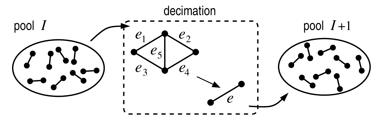
After has been initialized, all pools up to might be filled in this manner. Note that an edge effectively corresponds to a hierarchical graph , i.e. it has a “hidden” substructure that allows to represent a minimum-energy path with length . The attributes of the edge encode the characteristics of the respective path, i.e. its energy and length . A pool thus consists of instances of minimum-energy paths for hierarchical graphs at iteration step . Thereby, the computational resources needed to fill a pool stay constant as increases.

Further, each pool specifies its own distributions and of path energies and path lengths, respectively. These allow to quantify the scaling behavior of the average path length with system size as , defining the fractal dimension of the paths, the average path energy , and the fluctuation of the path energies as . Note that these energy fluctuations are measured with respect to the linear extension of the considered lattice graphs. This can be compared the ground-state energy fluctuations of the DPRM, which are commonly measured for polymers of a fixed length , giving rise to the fluctuation exponent defined as , see Ref. [3]. Hence, to compare our results with the DPRM case, one should rewrite the energy fluctuations as a function of the average path length . This leads to a corresponding estimate of via using the relation .
In the following section, we will use the algorithmic procedure outlined above in order to study the minimum-energy path problem for an increasing number of iteration steps and for a large range of values of the disorder parameter .
III Results
In the presented study, the disorder distribution is a Gaussian with mean and width . A tunable disorder parameter is defined as , so that the standard normal distribution is recovered in the limit . Typical values for the pool-size and iteration steps are and , respectively.
To facilitate intuition, note that as , typical minimum-energy paths will exhibit positive energies. Thus, an increasing path length will lead to an increasing path energy. Hence, a minimum-energy path will tend to be short in length. Considering hierarchical lattice graphs , one might consequently expect a scaling behavior , implying a scaling exponent . On the other hand, as , typical minimum-energy paths will exhibit negative energies. Therefore, an increasing path length results in a decreasing path energy, leading to expect , and therefore . In between these two extremal “trivial” cases, there exists a particular value of the disorder parameter that signifies the onset of “proliferation”, where as . Here the average path length exhibits a non-trivial scaling behavior displayed by a scaling exponent .
At first we attempt to estimate the value of by means of the secant method [39], considering different initial pools at a given value of . Next, we consider one particular initial pool to quantify the scaling behavior of the average minimum-energy path length and energy. Finally, we put under scrutiny the probability density of minimum-energy path energies.


III.1 Location of the critical point where the minimum-energy path energy vanishes
In order to approximate the critical point we considered pools of size and . So as to arrive at an estimate of at iteration step we proceeded as follows: Using the secant method we prepared a number of independent estimates of effective critical values , where at the considered value of . The distribution of these effective critical values (see inset of Fig. 4) is characterized by the average . E.g., at we yield , wherein the standard deviation among the independent estimates reads . The averages exhibit the scaling behavior , where a fit [40] to the interval yields , , and , see Fig. 4. The results did not depend much on the pool size, e.g. considering and proceeding as above we find and .
III.2 Trivial to non-trivial transition of the average minimum-energy path length

As it appears, for large values of and one should observe a vanishing average path energy. In the presented subsection we consider a single pool of size and in order to assess the scaling behavior of the minimum-energy path length and energy. For that pool we find that the average path energy changes its sign at (see inset of Fig. 5(a)). Further, at that approximate value the scaling behavior of the fluctuations related to the path energy and length change significantly (see Figs. 5(a),(b)). In this regard, the precise location of the peak position related to (see Fig. 5(b)) can be used to define an iteration-step dependent effective critical point . Seen as a function of , these effective critical points can be used to pinpoint the precise location where the proliferation transition of the path length occurs in the limit . The effective critical values exhibit a scaling of the form , where a fit to the interval yields the estimates , , and , see inset of Fig. 5(b). As pointed out above, for an increase in path length most likely results in an increasing path energy. Hence, one can expect that for the minimum-energy path problem investigated here effectively corresponds to the optimal path problem studied in Ref. [21], wherein a nonegative uniform disorder distribution was considered. From this it is immediate to expect , and for . From a direct fit to the scaling forms , and we obtained the numerical values for the scaling exponents , and (and consequently the “corrected” exponent ) as shown in Fig. 6 and listed in Tab. 1. For values of below and above the critical point, the fits were restricted to large iteration steps, i.e. . However, note that it is difficult to prepare a system right at : as increases, fluctuations will eventually cause the system to assume the asymptotic scaling behavior characteristic for or . Hence, in order to obtain the scaling exponents for the fitting procedure was restricted to intermediate iteration steps ( in case of ), only. Anyway, for the case of the energy, we actually require at , hence the value of right at the critical point is of limited relevance and a pure numerical artifact.
| 1 | 1 | 0.300(4) | 0.300(4) | |
| 1.158(1) | 0.3496(2) | 0.347(5) | 0.300(5) | |
| 1.5849631(1) | 1.58497(1) | 0.635(5) | 0.401(5) |
Another means to quantify the scaling behavior of the above observables is given by the local scaling exponents. E.g., denoting the average minimum-energy path length at a given value of and iteration step as , one can obtain the local analog to the fractal dimension as . The respective error can be obtained via error propagation as . The resulting local scaling exponents are shown in Fig. 7. The local equivalent of the energy fluctuation exponent can be computed in similar manner, see inset of Fig. 7. For a given value of and for increasing , the local exponents become independent of and tend to a limiting value that is within error bars in agreement with the numerical values of and listed in Tab. 1.

III.3 Importance sampling results for the ground-state energy distribution
As stressed above, for a disorder parameter the minimum energy path problem considered here effectively corresponds to the optimal path problem studied in Ref. [21]. This is further highlighted by the probability distribution function (pdf) of minimum-energy path energies. In this regard, Fig. 8 shows the simple-sampling estimate of the ground-state energy distribution for the minimum-energy path at for different iteration steps , obtained from pools of size . As evident from Fig. 8, data curves corresponding to different iteration steps scale according to
| (1) |
where defines a reduced energy with and describing the average and standard deviation of the distribution , respectively. This means that the scaling function does not depend on the value of . Note that the rescaled distribution of the optimal path energy for the case were edge-energies are drawn uniformly from the interval (i.e. the case considered in Ref. [21]) assumes the same scaling form and falls onto the same master curve.

Due to the close correspondence between the minimum-energy path problem studied here and DPRM problem one might expect that the scaling function has the shape of a Tracy-Widom distribution (see Refs. [41, 37]). The negative tail of the Tracy-Widom distribution exhibits the asymptotic scaling , where in case of the DPRM (having one space and one time direction) one has exactly [37]. The exponent , describing the negative tail of the pdf , is thereby related to the energy fluctuation exponent (listed in Tab. 1) by means of the expression . Furthermore, SAWs in quenched random hierarchical environments at the critical point were studied [27] using real-space renormalization techniques (quite similar to the approach presented here). Also in that case both tails of the scaling function are consistent with an exponential decay as given above. Under the assumption that the tails of the distribution reproduce under rescaling, they arrive at the estimates and for the negative and positive tail, respectively. However, their numerical results then did not allow to conclude with precise numerical estimates for the exponents .
Subsequently we address the question whether the distribution of ground-state energies in the minimum-energy path problem for , , and is consistent with a Tracy-Widom scaling form and we attempt to obtain a numerically precise estimate of the negative tail exponent for the above three cases. To this end, we consider an importance sampling procedure in the disorder [34, 35], where the sampling process is controlled by a guiding function [36]. This allows to compute the negative-energy tails of the ground-state energy distribution up to standard deviations away from its mean. Similar to Ref. [37] we consider the negative tails of the distribution for the reduced energy only. We further use a guiding function
| (2) |
in order to estimate the parameters that characterize best the simple sampling distributions at the three values . The respective estimates are listed in Tab. 2 and the guiding function for is indicated as dashed line in Fig. 8.
Let describe the true probability density function of observing a minimum-energy path with reduced energy for the model under consideration (bear in mind that it holds that , where ). In order to arrive at an ImSa estimate that approximates , we divide the generation of the iterations into two parts, consisting of and iterations, where is small, we consider or . The generation of the first iterations, is performed in the usual simple-sampling way, leading to a large () pool . The final iterations should be done in a way that also the interesting tails of the distribution are sampled. For this purpose, we generate a Markov chain of pools, which all are subsets of , but the sampling is done in a way that also the tails of the distribution of reduced energy values are sampled.
The initial pool is created by picking a (uniformly sampled) random subset of edges from . For this pool now the final levels of the hierarchy are performed within one graph: The edges comprising the sampling pool can be arranged into one particular realization of a hierarchical graph . Upon stepwise decimation this yields one particular edge with an edge energy and a corresponding reduced energy , wherein and describe the simple sampling estimate of . Note that the probability in the tails is very small, hence ImSa will not change and considerably.
The Markov chain Monte Carlo step reads as follows: From a given sampling pool we construct the next sampling pool using the following 2-step procedure:
- (1)
randomly choose a fraction of edges contained in the sampling pool and replace those edges by new edges chosen from the large pool . This then specifies a candidate for the next sampling pool, characterized by the reduced energy .
- (2)
set with probability
(3) Set otherwise.
To complete the importance sampling simulation, the evolution of the initial sampling pool is followed a number of steps. The resulting reduced energy values comprise an auxiliary distribution that describes the probability by means of which a reduced path energy is visited within the ImSa procedure. Since the importance sampling is designed such that a sampling pool having reduced energy is encountered with probability , the distribution is further given by the ratio (where describes the true pdf of observing a minimum-energy path with reduced energy for the considered model system). As long as the guiding function provides a reasonable approximation to the true distribution of path energies, the auxiliary distribution obtained using the IS procedure is rather “flat”. Thus, regarding the target distribution one might hope to improve on the negative-tail statistics provided by a simple sampling approach. As discussed in Ref. [36], successive configurations (i.e. sampling pools) encountered during an ImSa simulation are not independent. As a remedy one might consider the autocorrelation function
| (4) |
associated to the sequence of energy values obtained from the importance sampling procedure. The number of Monte Carlo steps that have to elapse until the autocorrelation function decays to gives the respective autocorrelation time . Sampling pools that are separated by Monte Carlo steps can be considered effectively uncorrelated. Finally, the truncated sequence of effectively uncorrelated energy values can be analyzed similar to the simple-sampling data.

The results discussed below were obtained for the choice , where we restricted the IS procedure to . We further performed a number of Monte Carlo steps to estimate the distribution of path energies in a target pool corresponding to . In order to assess the autocorrelation time we considered IS simulations at a disorder parameter and for and . As it appears, the autocorrelation function can be well described by a stretched exponential, i.e. , where . A best fit of that relation to the data yields the parameters and for , respectively. Such a stretched exponential might result from a continuous sum of pure exponential decays [42]. Further, a stretched exponential decay of the energy autocorrelation function was, above the respective critical temperature, also observed for the and fully frustrated Ising model [43]. To check whether there are different autocorrelation times relevant on different timescales of the ImSa simulation we performed the following analysis: we subdivided the “long” simulation run at into “shorter” runs, each of length . The runs of length are then considered as being independent and the characteristic autocorrelation time for the shorter sequences is estimated. In this regard, for it was sufficient to consider a pure power law fit-function. For values of larger than that, a stretched exponential turned out to be more adequate. As shown in the inset of Fig. 9, we found that for the effective autocorrelation time is well described by an algebraic dependence , whereas for the value of did not increase further, i.e. we observed . As pointed out above, sampling pools that are separated by more than Monte Carlo steps are effectively uncorrelated. One might now argue that, in order to use only uncorrelated values of to construct the distribution (and hence ), one should keep only every -th energy value. However, in Ref. [37] the authors concluded that if during the Monte Carlo steps the interval is crossed sufficiently often, it is not necessary to discard any energy values obtained during the IS simulation. Here, for , considering the interval and performing Monte Carlo steps at we found a number of interval crossings. In agreement with Ref. [37] we observed that it makes no difference whether the sequence of energy values collected during the IS procedure was truncated or not, the resulting pdf remained almost unchanged (apart from effects due to the different sample sizes used to construct the pdfs).


Below we present the results obtained for ImSa simulations at considering and a target distribution at (only the simulation at was carried out for a target pool at ). Once the distribution is obtained from the ImSa procedure, it can immediately be transformed to the desired pdf . A comparison of the SiSa and ImSa pdf shows that the absolute probabilities in the overlapping region do not coincide. This is due to the restriction of the relative energies to the interval during the ImSa simulation. One can easily account for this discrepancy by requiring that the SiSa and ImSa estimates coincide in the overlapping region, and by rescaling the ImSa estimate accordingly. In Figs. 10(a-c), the resulting pdfs of observing a minimum-energy path with reduced energy for are shown, respectively. Note that the pdfs are represented using histograms that consist of bins, each. In either case, the ImSa (SiSa) estimate is depicted for relative energies (). As evident from the figures, using the ImSa procedure probabilities as small as can be reached, in contrast to for a SiSa approach, cf. Fig. 8. The insets to Figs. 10(a-c) indicate the normalized deviation of a best fit of the function to the negative tail of . Once the fit is performed the deviation is obtained as , where indicates the measurement error on as obtained by bootstrap resampling [40]. The observation that (considering a fit of to the ImSa data) is of order one and changes sign in an irregular fashion indicates that there are no systematic deviations and that the fit-function represents a proper approximation to the negative tail of the observed pdf. In particular, Fig. 10(a) highlights that a fit to the SiSa pdf might be misleading if one is interested in the true scaling behavior of as . For that purpose, the above fit-function with fitting parameters obtained for the SiSa data (dashed curve in the main plot) was used to compute the normalized deviation to the ImSa data (dashed line in the inset). Referring to this one finds rather strong systematic deviations where, e.g., . The parameters that correspond to a best fit to the ImSa data are listed in Tab. 3.
As pointed out above, previous studies suggested that the exponent is related to the energy fluctuation exponent (listed in Tab. 1) by means of the expression . Here, for the minimum-energy path problem on hierarchical lattice graphs we find that this expression holds for all values of thus considered. To facilitate comparison, the values are listed in Tab. 3.
IV Conclusions
In the presented article we have investigated a particular MWP problem on MK hierarchical graphs. It is quite similar to earlier polymer [2, 26, 3, 27, 28, 29, 31] and optimal path problems [6, 21, 32, 33]. The important difference is that for a considerable fraction of negative edge energies, the total energy of a path may be reduced by taking longer paths (which leads to a different universality class). In the same fashion as the optimal path problem on hierarchical graphs, studied in Ref. [21], corresponds to the (generic) non-directed optimal path problem [10], the minimum-energy path problem studied here corresponds to the negative-energy percolation problem [13] in which there is a path forced onto the system and where the disorder is “weak” enough to render the appearance of loops irrelevant for the scaling behavior of the path.
Here, the scaling properties of the MWP obtained after the decimation of huge hierarchical graphs change with increasing edge-disorder, leading from a phase where the path displays a self-affine scaling behavior to a phase where the path displays a (statistically) self-similar scaling behavior. We characterized the respective phase transition by monitoring the length and energy of the MWPs as function of the disorder and quantified the scaling behavior of the observables (and their fluctuations) by means of proper critical exponents. While the scaling of the observables off criticality can be explained intuitively, the scaling behavior found at the critical point of the model is nontrivial and compares well to the scaling observed for the optimal path problem on the same hierarchical lattice in the limit of “strong” disorder [21]. However, note that the precise optimization criteria of both models are slightly different: while in the optimal path problem [21, 10] one aims to minimize the largest energy along a sub-path, here one strives after minimizing the sum of energies along a sub-path. Note that this was already realized for the respective models on regular lattice graphs, where quite similar scaling exponents for the average path length were found in dimensions through , see Ref. [15].
Further, we performed an importance sampling simulation for the ground-state energy distribution of the paths and confirmed that it is consistent with a Tracy-Widom scaling form, similar to the directed polymer in a random medium [37]). Using the importance sampling procedure allowed for an analysis of the ground-state energy distribution down to probabilities as small as (in contrast, a convenient simple sampling approach only allows to reach ), i.e. up to standard deviations away from the mean of the respective distribution. This leads to a precise estimate of the scaling behavior of the negative tail of the ground-state energy distribution. For all values of the disorder parameter considered here, the respective exponents could be related to the energy-fluctuation exponents via the relation .
Acknowledgements.
OM acknowledges financial support from the DFG (Deutsche Forschungsgemeinschaft) under grant HA3169/3-1. The simulations were performed at the HPC Cluster HERO, located at the University of Oldenburg (Germany) and funded by the DFG through its Major Instrumentation Programme (INST 184/108-1 FUGG) and the Ministry of Science and Culture (MWK) of the Lower Saxony State.References
- [1] K. Kremer, Z. Phys. B 45, 149 (1981).
- [2] M. Kardar and Y. C. Zhang, Phys. Rev. Lett. 58, 2087 (1987).
- [3] B. Derrida, Physica A 163, 71 (1990).
- [4] P. Grassberger, J. Phys. A 26, 1023 (1993).
- [5] R. Parshani, L. A. Braunstein, and S. Havlin, Phys. Rev. E 79, 050102 (2009).
- [6] M. Cieplak, A. Maritan, and J. R. Banavar, Phys. Rev. Lett. 72, 2320 (1994).
- [7] O. Melchert and A. K. Hartmann, Phys. Rev. B 76, 174411 (2007).
- [8] O. Melchert and A. K. Hartmann, Comp. Phys. Comm. 182, 1828 (2011).
- [9] K. Schwarz, A. Karrenbauer, G. Schehr, and H. Rieger, J. Stat. Mech. 2009, P08022 (2009).
- [10] N. Schwartz, A. L. Nazaryev, and S. Havlin, Phys. Rev. E 58, 7642 (1998).
- [11] T. H. Cormen, C. E. Leiserson, R. L. Rivest, and C. Stein, Introduction to Algorithms, 2nd edition (MIT Press, 2001).
- [12] O. Melchert and A. K. Hartmann, Phys. Rev. B 79, 184402 (2009).
- [13] O. Melchert and A. K. Hartmann, New. J. Phys. 10, 043039 (2008).
- [14] L. Apolo, O. Melchert, and A. K. Hartmann, Phys. Rev. E 79, 031103 (2009).
- [15] O. Melchert, L. Apolo, and A. K. Hartmann, Phys. Rev. E 81, 051108 (2010).
- [16] O. Melchert, A. K. Hartmann, and M. Mézard, Phys. Rev. E 84, 041106 (2011).
- [17] C. Norrenbrock, O. Melchert, and A. K. Hartmann (2012), preprint: arXiv:1205.1412.
- [18] G. Claussen, L. Apolo, O. Melchert, and A. K. Hartmann, Phys. Rev. E 86, 056708 (2012).
- [19] R. K. Ahuja, T. L. Magnanti, and J. B. Orlin, Network Flows: Theory, Algorithms, and Applications (Prentice Hall, 1993).
- [20] D. Stauffer and A. Aharony, Introduction to Percolation Theory (Taylor and Francis, London, 1994).
- [21] M. Cieplak, A. Maritan, M. R. Swift, A. Ahattacharya, A. L. Stella, and J. R. Banavar, J. Phys. A 28, 5693 (1995).
- [22] O. R. Salmon, B. T. Agostini, and F. D. Nobre, Phys. Lett. A 374, 1631 (2010).
- [23] R. Teodoro, C. G. Bezerra, A. M. Mariz, and F. A. da Costa, Preprint: arXiv:1005.3863v1 (2010).
- [24] A. J. Bray and S. Feng, Phys. Rev. B 36, 8456 (1987).
- [25] S. Boettcher, Eur. Phys. J. B 33, 439 (2003).
- [26] B. Derrida and R. B. Griffiths, Europhys. Lett. 8, 111 (1989).
- [27] P. Doussal and J. Machta, J. Stat. Phys. 64, 541–578 (1991).
- [28] P. Devillard, Phys. Rev. Lett. 70, 1124 (1993).
- [29] M. S. Cao, J. Stat. Phys. 71, 51 (1993).
- [30] Y. Shussman and A. Aharony, J. Stat. Phys. 80, 147 (1995).
- [31] C. Monthus and T. Garel, Phys. Rev. E 77, 021132 (2008).
- [32] A. Hansen and J. Kertész, Phys. Rev. Lett. 93, 040601 (2004).
- [33] S. V. Buldyrev, S. Havlin, and H. E. Stanley, Phys. Rev. E 73 (2006).
- [34] A. K. Hartmann, Phys. Rev. E 65, 056102 (2002).
- [35] A. Engel, R. Monasson, and A. K. Hartmann, J. Stat. Phys. 117, 387 (2004).
- [36] M. Körner, H. G. Katzgraber, and A. K. Hartmann, J. Stat. Mech. p. P04005 (2006).
- [37] C. Monthus and T. Garel, Phys. Rev. E 74, 051109 (2006).
- [38] S. Wolfsheimer, B. Burghardt, and A. K. Hartmann, Algorithms for Molecular Biology 2, 9 (2007).
- [39] W. H. Press, S. A. Teukolsky, W. T. Vetterling, and B. P. Flannery, Numerical Recipes in C (Cambridge University Press, Cambridge, U.K., 1992).
- [40] A. K. Hartmann, Practical Guide to Computer Simulations (World Scientific, Singapore, 2009).
- [41] T. Halpin-Healy and Y.-C. Zhang, Phys. Rep. 254, 215 (1995).
- [42] D. C. Johnston, Phys. Rev. B 74, 184430 (2006).
- [43] G. Franzese, A. Fierro, A. De Candia, and A. Coniglio, Physica A 257, 376 (1998).