跳到论文正文
W Papers独立论文阅读器 arXiv:1302.6326 论文正文 计算阅读时间 · 0%
引用这篇论文根据当前论文元数据生成,正式投稿前建议核对。


License: arXiv.org perpetual non-exclusive license
arXiv:1302.6326v1 [math.NA] 26 Feb 2013

Moment-based cosh-Hilbert Inversion and Its Applications in Single-photon Emission Computed Tomography

Shousheng Luo      Jiansheng Yang      Tie Zhou Affiliation: LMAM, School of Mathematical Sciences, Peking University, Beijing 100871, China

Abstract: The inversion of cosh-Hilbert transform (CHT) is one of the most crucial steps for single-photon emission computed tomography with uniform attenuation from truncated projection data. Although the uniqueness of the CHT inversion had been proved [1], there is no exact and analytic inverse formula so far. Several approximated inversion algorithms of the CHT had been developed [1][2]. In this paper, we proposed a new numerical moment-based inversion algorithm.

1 Introduction

Single-photon emission computed tomography(SPECT) is a non-invasive diagnostic technology in nuclear medicine. It is used to image the physiological function of various organs with the help of radiopharmaceutical, a biochemical molecular labeled by radioisotope. Radiopharmaceutical is induced into a patient, and the emitted gamma photons, attenuated by the body, are measured by a gamma camera rotating around it. The task of SPECT reconstruction is to estimate the radiopharmaceutical distribution from the measured data.
From the mathematical point of view, the two-dimensional(2D) SPECT reconstruction problem is to inverse the attenuated Radon transform(aRt) of pp [3],

g(s,ϕ)=Rμp(s,ϕ)=∫ℝp(sθ+tθ⟂)e−∫t∞μ(sθ+τθ⟂)dτdt,\displaystyle g(s,\phi)=R_{\mu}{p}(s,\phi)=\int_{\mathbb{R}}p(s\theta+t\theta^{\perp})e^{-\int_{t}^{\infty}\mu(s\theta+\tau\theta^{\perp}){d\tau}}dt, (1)

where p⁡(x)p(x) and μ⁡(x)\mu(x) denote the distribution of radiopharmaceutical and the attenuation coefficient of gamma photon at x=(x1,x2)x=(x_{1},x_{2}). Further, θ=(cos⁡ϕ,sin⁡ϕ)\theta=(\cos\phi,\sin\phi) and θ⟂=(−sin⁡ϕ,cos⁡ϕ)\theta^{\perp}=(-\sin\phi,\cos\phi) denote two perpendicular vectors. Although pp is a function with a compact support Ω\Omega in practice, the integral (1) is written over (−∞,+∞)(-\infty,+\infty) for convenience.
If μ=0\mu=0, the aRt formula (1) is the well-known Radon transform(Rt), which is the mathematical basis of computed tomography(CT). We can inverse Rt by the filtering back-projection(FBP) formula [3] from 180∘ projection data due to the relation that (R​p)​(−s,ϕ+π)=(R​p)​(s,ϕ)(R{p})(-s,\phi+\pi)=(R{p})(s,\phi), where RR denotes the Radon transform. If μ≠0\mu\neq 0, the filtering back-projection formula for aRt was firstly discovered by the author of [4] (Latter, a simpler deviation was illustrated in [5]).
In this paper, we are interested in a special case of aRt, which assumes that the attenuation map μ\mu is an uniform constant in the convex domain including the support of pp. With the assumption that μ⁡(x)=μ0\mu(x)=\mu_{0}(constant) inside Ω\Omega and μ⁡(x)=0\mu(x)=0 outside Ω\Omega, the reconstruction of pp is equivalent to solving the exponential Radon transform(eRt) of pp (See [6][3] for details)

g⁡(s,ϕ)=Rμ0​p​(s,ϕ)=∫ℝp⁡(s​θ+t​θ⟂)​eμ0​t​𝑑t\displaystyle g(s,\phi)=R_{\mu_{0}}p(s,\phi)=\int_{\mathbb{R}}p(s\theta+t\theta^{\perp})e^{\mu_{0}t}dt (2)

Since the exponential Radon transform does not have the parity property of the Radon transform, i.e. (Rμ0​p)​(−s,ϕ+π)≠(Rμ0​p)​(s,ϕ)(R_{\mu_{0}}{p})(-s,\phi+\pi)\neq(R_{\mu_{0}}{p})(s,\phi) for μ0≠0\mu_{0}\neq 0, it is a long-standing opinion that 2​π2\pi data is necessary for the reconstruction of pp. However, accurate reconstruction from non-truncated projections known only over 180∘ was shown to be possible for any value of μ0\mu_{0} [7, 8].
Because of practical constraints due to the imaging hardware, scanning geometry, or ionizing radiation exposure, the projection data are not theoretically sufficient for exact image reconstruction. One of the important case is the truncated data that the projection data g⁡(ϕ,s)g(\phi,s) are only known for a limited range of ss. For example, if Ω\Omega is the centered disc of radius RR, the projection data is truncated as long as g⁡(ϕ,s)g(\phi,s) is not known for all s∈[−R,R]s\in[-R,R].
An explicit formula was suggested in [9], in which the author reduced the reconstruction of 2D SPECT to solving a one-dimensional integral equation called cosh-weighted Hilbert transform(CHT) by the weight-differential backprojection of eRt. This method further was developed further in [1], in which the author proved a similar result of the classic Radon transform. Recently, this result was extended to developed the reconstruction of three-dimensional(3D) SPECT with uniform attenuation[10]. More importantly, this method can be used to conduct the reconstruction of region-of-interesting from truncated projection data [1, 9]. However, there is no explicit formula for CHT so far. Several numerical algorithms of the CHT have been proposed [1, 2, 9].
In this paper, we propose a moment-based method to solve the CHT numerically. In this proposed approach, the solution of CHT is represented as the result of Tricomi formula for Hilbert transform followed by a correction term, which is related to the moments of the underlying function. The numerical simulations show that the proposed method can solve the CHT efficiently for a large range of the attenuation constant μ0\mu_{0}.
The rest of this paper is organized as follow. We review the derivation of cosh-weighted Hilbert transform, and present the moment-based method in section 2. Numerical experiments are shown in section 3. Some discussions and conclusions are given in section 4. And the appendix A is devoted to some numerical techniques.

2 Cosh-weighted Hilbert Transform and the Proposed Method

This section consists of two parts. We firstly review the derivation of cosh-weighted Hilbert transform(CHT) from the exponential Radon transform[1][9]. Then, the moment-based method is given.

2.1 Review of Cosh-weighted Hilbert Transform

The basic idea is similar to differential back-projection of Radon transform (μ0=0\mu_{0}=0), but with a weight function. Let b⁡(x)b(x) be defined as

b(x)=∫0πe−μ0x⋅θ⟂(Rμ0′p)(x⋅θ,ϕ)dϕ,b({x})=\int_{0}^{\pi}{e^{-\mu_{0}x\cdot{\theta}^{\perp}}}(R_{\mu_{0}}^{\prime}{p})(x\cdot\theta,\phi)d\phi, (3)

where the derivative is respect to the first variable of Rμ0​pR_{\mu_{0}}p, i.e., (Rμ0′​p)​(s,ϕ)=∂∂s​(Rμ0​p)​(s,ϕ)(R_{\mu_{0}}^{\prime}{p})(s,\phi)={{\partial}\over{\partial{s}}}(R_{\mu_{0}}{p})(s,\phi), and x⋅θx\cdot\theta denotes the standard inner product of ℝ2\mathbb{R}^{2}. By the definition of eRt (2), interchanging the partial derivative with the integration and applying the chain rule, we can obtain

(Rμ0′​p)​(s,ϕ)=∫ℝeμ0​t′​θ⋅∇p​(s​θ+t′​θ⟂)​d​t′.(R_{\mu_{0}}^{\prime}{p})(s,\phi)=\int_{\mathbb{R}}{e^{\mu_{0}t^{\prime}}}\theta\cdot\nabla{p}(s\theta+t^{\prime}\theta^{\perp})dt^{\prime}.

Here, we assume that pp is continuously differentiable. Since x=(x⋅θ)​θ+(x⋅θ⟂)​θ⟂x=(x\cdot\theta)\theta+(x\cdot\theta^{\perp})\theta^{\perp}, we have that

(Rμ0′​p)​(x⋅θ,ϕ)\displaystyle(R_{\mu_{0}}^{\prime}{p})({x}\cdot\theta,\phi) =\displaystyle= ∫ℝeμ0​t′​θ⋅∇p​((x⋅θ)​θ+t′​θ⟂)​d​t′\displaystyle\int_{\mathbb{R}}{e^{\mu_{0}{t}^{\prime}}}\theta\cdot\nabla{p}((x\cdot\theta)\theta+t^{\prime}\theta^{\perp})dt^{\prime} (4)
=\displaystyle= ∫ℝeμ0​t′​θ⋅∇p​(x+(t′−x⋅θ⟂)​θ⟂)​d​t′\displaystyle\int_{\mathbb{R}}{e^{\mu_{0}{t}^{\prime}}}\theta\cdot\nabla{p}({x}+(t^{\prime}-{x}\cdot\theta^{\perp})\theta^{\perp})dt^{\prime}
=\displaystyle= eμ0​x⋅θ​∫ℝeμ0​t​θ⋅∇p​(x+t​θ⟂)​𝑑t\displaystyle e^{\mu_{0}{x}\cdot\theta}\int_{\mathbb{R}}{e^{\mu_{0}{t}}}\theta\cdot\nabla{p}(x+t\theta^{\perp})dt
=\displaystyle= −eμ0​x⋅θ∫ℝeμ0​tt∂∂ϕp(x+tθ⟂)dt,\displaystyle-e^{\mu_{0}{x}\cdot\theta}\int_{\mathbb{R}}{{e^{\mu_{0}{t}}}\over{t}}{{\partial}\over{\partial\phi}}p(x+t\theta^{\perp})dt,

where we use a variable replacement of t=t′−x⋅θt=t^{\prime}-{x}\cdot\theta for the third equality, and the last equality is implied by

∂∂ϕ​p​(x+t​θ⟂)\displaystyle{{\partial}\over{\partial\phi}}p(x+t\theta^{\perp}) =\displaystyle= ∇p​(x+t​θ⟂)⋅(t​∂∂ϕ​θ⟂)\displaystyle\nabla{p(x+t\theta^{\perp})}\cdot(t{{\partial}\over{\partial\phi}}\theta^{\perp})
=\displaystyle= −tθ⋅∇p(x+tθ⟂).\displaystyle-t\theta\cdot\nabla{p(x+t\theta^{\perp})}.

Inserting (4) into (3) and interchanging the order of intergation, we have that

b⁡(x)\displaystyle b({x}) =\displaystyle= −∫ℝeμ0​ttp(x+tθ⟂)|dπ0t\displaystyle-\int_{\mathbb{R}}{{e^{\mu_{0}{t}}}\over{t}}p(x+t\theta^{\perp})\left|{}_{0}^{\pi}{dt}\right. (5)
=\displaystyle= −∫ℝeμ0​tt[p(x1,x2−t)−p(x1,x2+t)]dt\displaystyle-\int_{\mathbb{R}}{{e^{\mu_{0}{t}}}\over{t}}\left[p(x_{1},x_{2}-t)-p(x_{1},x_{2}+t)\right]dt
=\displaystyle= −∫ℝeμ0​ttp(x1,x2−t)dt+∫ℝeμ0​ttp(x1,x2+t)dt\displaystyle-\int_{\mathbb{R}}{{e^{\mu_{0}{t}}}\over{t}}p(x_{1},x_{2}-t)dt+\int_{\mathbb{R}}{{e^{\mu_{0}{t}}}\over{t}}p(x_{1},x_{2}+t)dt
=\displaystyle= −2π∫ℝcosh⁡μ0​(x2−x2′)π⁡(x1−x2′)p(x1,x2′)dx2′,\displaystyle-2\pi\int_{\mathbb{R}}{{\cosh{\mu_{0}(x_{2}-x_{2}^{\prime})}}\over{\pi(x_{1}-x_{2}^{\prime})}}p(x_{1},x_{2}^{\prime})dx_{2}^{\prime}, (6)

where we use variable replacements of x2′=x2−tx_{2}^{\prime}=x_{2}-t and x2′=x2+tx_{2}^{\prime}=x_{2}+t for the first and second terms of (5), respectively. The above integrals (5) and (6) are understood in the sense of Cauchy principal value. In fact, we are only interested in the reconstruction of pp at (x1,x2)∈Ω(x_{1},x_{2})\in\Omega, a bounded and convex region outside which pp is known to be zero. Denoting by (x1,L⁡(x1))(x_{1},L(x_{1})) and (x1,U⁡(x1))(x_{1},U(x_{1})) the end points of the intersection of Ω\Omega with the line parallel to the x2x_{2}-axis through the point (x1,x2)∈Ω(x_{1},x_{2})\in\Omega, we have

b(x1,x2)=−2π∫L⁡(x1)U⁡(x1)cosh⁡μ0​(x2−x2′)π⁡(x2−x2′)p(x1,x2′)dx2′\displaystyle b(x_{1},x_{2})=-2\pi\int_{L(x_{1})}^{U(x_{1})}{{\cosh{\mu_{0}(x_{2}-x_{2}^{\prime})}}\over{\pi(x_{2}-x_{2}^{\prime})}}p(x_{1},x_{2}^{\prime})dx_{2}^{\prime} (7)

If Ω\Omega is a centered disc of radius RR, we have U⁡(x1)=−L⁡(x1)=R2−x12U(x_{1})=-L(x_{1})=\sqrt{R^{2}-x_{1}^{2}}.
Therefore, the SPECT reconstruction problem is changed into solving the so-called finite cosh-weighted Hilbert transform along each vertical line with (Rμ0​p)​(x1,0)(R_{\mu_{0}}p)(x_{1},0) and (Rμ0​p)​(−x1,π)(R_{\mu_{0}}p)(-x_{1},\pi) known.
For simplicity, we focus on the following standard form: reconstruct a function f⁡(t)f(t) with its support supp​(f)⊂(−1,1)\text{supp}{(f)}\subset(-1,1) from its finite cosh-weighted Hilbert transform

hμ1​(τ)\displaystyle h_{\mu_{1}}(\tau) =\displaystyle= ∫−11cosh⁡μ1​(τ−t)π⁡(τ−t)f(t)dt, |τ|<1\displaystyle\int_{-1}^{1}{{\cosh{\mu_{1}(\tau-t)}}\over{\pi(\tau-t)}}f(t)dt,\text{\indent\ }|\tau|<1 (8)

with cμ1=∫−11f⁡(t)​cosh⁡(μ1​t)​𝑑tc_{\mu_{1}}=\int_{-1}^{1}f(t)\cosh({\mu_{1}t})dt known. We can normalize the general form of (6) as the standard form by using the following affine transformation

μ1\displaystyle\mu_{1} =\displaystyle= d^​μ0,\displaystyle\hat{d}\mu_{0},
f⁡(τ)\displaystyle f(\tau) =\displaystyle= p⁡(x1,c^+d^​τ),\displaystyle p(x_{1},\hat{c}+\hat{d}\tau),
hμ1​(t)\displaystyle h_{\mu_{1}}(t) =\displaystyle= −12​d^​π​b​(x1,c^+d^​τ),\displaystyle-{1\over 2\hat{d}\pi}b(x_{1},\hat{c}+\hat{d}\tau),

where c^=U⁡(x1)+L⁡(x1)2\hat{c}={U(x_{1})+L(x_{1})\over 2} and d^=U⁡(x1)−L⁡(x1)2\hat{d}=\frac{U(x_{1})-L(x_{1})}{2}. Further, we have

cμ1=1d^​[e−c^​μ0​(Rμ0​p)​(x1,0)+ec^​μ0​(Rμ0​p)​(−x1,π)].\displaystyle c_{\mu_{1}}=\frac{1}{\hat{d}}\left[e^{-\hat{c}\mu_{0}}(R_{\mu_{0}}p)(x_{1},0)+e^{\hat{c}\mu_{0}}(R_{\mu_{0}}p)(-x_{1},\pi)\right].

If μ1=0\mu_{1}=0, by the Tricomi formula [11], we have

f⁡(t)​1−t2\displaystyle f(t)\sqrt{1-t^{2}} =\displaystyle= c0π−∫−111−s2π⁡(t−s)​h0​(s)​𝑑s\displaystyle{{c_{0}}\over{\pi}}-\int_{-1}^{1}{\sqrt{1-s^{2}}\over{\pi(t-s)}}h_{0}(s)ds (9)

Then, we can obtain ff for |t|<1|t|<1 by dividing 1−t2\sqrt{1-t^{2}} on both sides of (9).

2.2 Moment-based Method

In this subsection, we focus on the inverse of the finite cosh-weighted Hilbert transform (8). For the sake of reference, we introduce some notations firstly.

hm​(t)\displaystyle h_{m}(t) =\displaystyle= 1π​∫−11(t−τ)m−1​f​(τ)​𝑑τ,\displaystyle{1\over\pi}\int_{-1}^{1}(t-\tau)^{m-1}f(\tau)d\tau,
Tn​(t)\displaystyle T_{n}(t) =\displaystyle= 1π​∫−111−s2t−s​sn​𝑑s,\displaystyle{1\over\pi}\int_{-1}^{1}{\sqrt{1-s^{2}}\over{t-s}}s^{n}ds,
Tij\displaystyle T_{i}^{j} =\displaystyle= 1π​∫−11tj1−t2​Ti​(t)​𝑑t,\displaystyle{1\over\pi}\int_{-1}^{1}\frac{t^{j}}{\sqrt{1-t^{2}}}T_{i}(t)dt,

and the mm-th moment cm=∫−11f⁡(t)​tm​𝑑tc_{m}=\int_{-1}^{1}f(t)t^{m}dt of ff. Obviously, we have that Tn​(−t)=(−1)n+1​Tn​(t)T_{n}(-t)=(-1)^{n+1}T_{n}(t).
By the Taylor expansion of the function coshμ1t\cosh\mu_{1}t, we have

hμ1​(t)\displaystyle h_{\mu_{1}}(t) =\displaystyle= 1π​∫−11[1t−τ​f​(τ)+∑k=1∞μ12​k(2​k)!​(t−τ)2​k−1​f​(τ)]​𝑑τ\displaystyle{1\over\pi}\int_{-1}^{1}\left[{1\over{t-\tau}}f(\tau)+\sum\limits_{k=1}^{\infty}{\mu_{1}^{2k}\over{(2k)!}}(t-\tau)^{2k-1}f(\tau)\right]d\tau (10)
=\displaystyle= h0​(t)+∑k=1∞μ12​k(2​k)!​h2​k​(t),\displaystyle h_{0}(t)+\sum\limits_{k=1}^{\infty}{\mu_{1}^{2k}\over{(2k)!}}{h_{2k}}(t),

and

cμ1\displaystyle c_{\mu_{1}} =\displaystyle= ∫−11cosh⁡(μ1​t)​f​(t)​𝑑t\displaystyle\int_{-1}^{1}\cosh(\mu_{1}{t})f(t)dt (11)
=\displaystyle= c0+∑k=1∞μ12​k(2​k)!​c2​k.\displaystyle c_{0}+\sum\limits_{k=1}^{\infty}{\mu_{1}^{2k}\over{(2k)!}}{c_{2k}}.

Therefore, h0​(t)h_{0}(t) and c0c_{0} can be represented by h0​(t)=hμ1​(t)−∑k=1∞μ12​k(2​k)!​h2​k​(t)h_{0}(t)=h_{\mu_{1}}(t)-\sum\limits_{k=1}^{\infty}{\mu_{1}^{2k}\over{(2k)!}}{h_{2k}}(t), c0=cμ1−∑k=1∞μ12​k(2​k)!​c2​k.c_{0}=c_{\mu_{1}}-\sum\limits_{k=1}^{\infty}{\mu_{1}^{2k}\over{(2k)!}}{c_{2k}}. Applying the Tricomi formula for the finite Hilbert transform[11], we have

f⁡(t)​1−t2\displaystyle f(t){\sqrt{1-t^{2}}} (12)
=\displaystyle= 1π​(cμ1−∑k=1∞μ12​k(2​k)!​c2​k)−1π​∫−111−τ2t−τ​(hμ1​(τ)−∑k=1∞μ12​k(2​k)!​h2​k​(τ))​𝑑τ\displaystyle{1\over\pi}(c_{\mu_{1}}-\sum\limits_{k=1}^{\infty}{\mu_{1}^{2k}\over{(2k)!}}{c_{2k}})-{{1}\over{\pi}}\int_{-1}^{1}{{\sqrt{1-\tau^{2}}}\over{t-\tau}}\left(h_{\mu_{1}}(\tau)-\sum\limits_{k=1}^{\infty}{\mu_{1}^{2k}\over{(2k)!}}{h_{2k}}(\tau)\right)d\tau
=\displaystyle= fμ1​(t)−1π​∑k=1∞μ12​k(2​k)!​c2​k+1π2​∑k=1∞μ12​k(2​k)!​∫−111−τ2t−τ​∫−11(τ−s)2​k−1​f​(s)​𝑑s​𝑑τ\displaystyle f_{\mu_{1}}(t)-{{1}\over{\pi}}\sum\limits_{k=1}^{\infty}{\mu_{1}^{2k}\over{(2k)!}}{c_{2k}}+{1\over{\pi^{2}}}\sum\limits_{k=1}^{\infty}{\mu_{1}^{2k}\over{(2k)!}}\int_{-1}^{1}{{\sqrt{1-\tau^{2}}}\over{t-\tau}}\int_{-1}^{1}(\tau-s)^{2k-1}f(s)dsd\tau
=\displaystyle= fμ1​(t)−1π​∑k=1∞μ12​k(2​k)!​c2​k+1π2​∑k=1∞μ12​k(2​k)!​∫−11f⁡(s)​∫−111−τ2t−τ​(τ−s)2​k−1​𝑑τ​𝑑s,\displaystyle f_{\mu_{1}}(t)-{{1}\over{\pi}}\sum\limits_{k=1}^{\infty}{\mu_{1}^{2k}\over{(2k)!}}{c_{2k}}+{1\over{\pi^{2}}}\sum\limits_{k=1}^{\infty}{\mu_{1}^{2k}\over{(2k)!}}\int_{-1}^{1}f(s)\int_{-1}^{1}{{\sqrt{1-\tau^{2}}}\over{t-\tau}}(\tau-s)^{2k-1}d\tau ds,
=\displaystyle= fμ1​(t)−1π​∑k=1∞μ12​k(2​k)!​c2​k+1π2​∑k=1∞μ12​k(2​k)!​∑l=02​k−1A2​k−1l​∫−11f⁡(s)​(−s)l​∫−111−τ2t−τ​τ2​k−1−l​𝑑τ​𝑑s\displaystyle f_{\mu_{1}}(t)-{{1}\over{\pi}}\sum\limits_{k=1}^{\infty}{\mu_{1}^{2k}\over{(2k)!}}{c_{2k}}+{1\over{\pi^{2}}}\sum\limits_{k=1}^{\infty}{\mu_{1}^{2k}\over{(2k)!}}\sum\limits_{l=0}^{2k-1}A_{2k-1}^{l}\int_{-1}^{1}f(s)(-s)^{l}\int_{-1}^{1}{{\sqrt{1-\tau^{2}}}\over{t-\tau}}\tau^{2k-1-l}d\tau ds
=\displaystyle= fμ1​(t)−1π​∑k=1∞μ12​k(2​k)!​c2​k+1π​∑k=1∞μ12​k(2​k)!​∑l=02​k−1A2​k−1l​(−1)l​cl​T2​k−1−l​(t),\displaystyle f_{\mu_{1}}(t)-{{1}\over{\pi}}\sum\limits_{k=1}^{\infty}{\mu_{1}^{2k}\over{(2k)!}}{c_{2k}}+{1\over{\pi}}\sum\limits_{k=1}^{\infty}{\mu_{1}^{2k}\over{(2k)!}}\sum\limits_{l=0}^{2k-1}A_{2k-1}^{l}(-1)^{l}c_{l}T_{2k-1-l}(t),

where fμ1​(t)=1π​(cμ1−∫−111−τ2t−τ​hμ1​(τ)​𝑑τ)f_{\mu_{1}}(t)={1\over\pi}(c_{\mu_{1}}-\int_{-1}^{1}{{\sqrt{1-\tau^{2}}}\over{t-\tau}}h_{\mu_{1}}(\tau)d\tau) and Anm=n!m!​(n−m)!A_{n}^{m}=\frac{n!}{m!(n-m)!}. The equation (12) provides us a relationship between the moments of ff and fμ1f_{\mu_{1}}, which tells us that we can reconstruct ff accurately if the moments of ff are known.
Define dn=∫−11tn1−t2​fμ1​(t)​𝑑td_{n}=\int_{-1}^{1}{t^{n}\over\sqrt{1-t^{2}}}f_{\mu_{1}}(t)dt firstly. Multiplying t2​i1−t2\frac{t^{2i}}{\sqrt{1-t^{2}}}( i=0,1,2,⋯,∞i=0,1,2,\cdots,\infty) on both sides of (12), and integrating on the interval (−1,1)(-1,1), we have that

c2​i\displaystyle c_{2i} =\displaystyle= ∫−11f⁡(t)​t2​i​𝑑t\displaystyle\int_{-1}^{1}f(t)t^{2i}dt (13)
=\displaystyle= ∫−11fμ1​(t)​t2​i1−t2​𝑑t−(∫−11t2​i1−t2​𝑑t)​∑k=1∞μ12​k(2​k)!​c2​k+1π​∑k=1∞μ12​k(2​k)!​∑l=02​k−1A2​k−1l​(−1)l​cl​(1π​∫−11T2​k−1−l​(t)​t2​i1−t2​𝑑t)\displaystyle\int_{-1}^{1}\frac{f_{\mu_{1}}(t)t^{2i}}{\sqrt{1-t^{2}}}dt-\left(\int_{-1}^{1}\frac{t^{2i}}{\sqrt{1-t^{2}}}dt\right)\sum\limits_{k=1}^{\infty}{\mu_{1}^{2k}\over{(2k)!}}c_{2k}+{1\over{\pi}}\sum\limits_{k=1}^{\infty}{\mu_{1}^{2k}\over{(2k)!}}\sum\limits_{l=0}^{2k-1}A_{2k-1}^{l}(-1)^{l}c_{l}\left({1\over\pi}\int_{-1}^{1}{T_{2k-1-l}(t)t^{2i}\over{\sqrt{1-t^{2}}}}dt\right)
=\displaystyle= d2​i−B2​i​∑k=1∞μ12​k(2​k)!​c2​k+∑k=1∞μ12​k(2​k)!​∑l=0k−1A2​k−12​l​T2​(k−l)−12​i​c2​l,\displaystyle d_{2i}-B_{2i}\sum\limits_{k=1}^{\infty}{\mu_{1}^{2k}\over{(2k)!}}c_{2k}+\sum\limits_{k=1}^{\infty}{\mu_{1}^{2k}\over{(2k)!}}\sum\limits_{l=0}^{k-1}A_{2k-1}^{2l}T_{2(k-l)-1}^{2i}c_{2l},

where B2​i=1π​∫−11t2​i1−t2​𝑑t=1π​∫−π2π2sin2​i⁡α​𝑑α=(2​i−1)!!(2​i)!!B_{2i}={1\over\pi}\int_{-1}^{1}\frac{t^{2i}}{\sqrt{1-t^{2}}}dt={1\over\pi}\int_{-\frac{\pi}{2}}^{\frac{\pi}{2}}\sin^{2i}\alpha{d\alpha}=\frac{(2i-1)!!}{(2i)!!} for i>0i>0, and B0=1B_{0}=1. The second equality is implied by the uniform convergence of the series, and the third equality holds because T2​k​(t)T_{2k}(t) is an odd function for all kk by the definition of Tn​(t)T_{n}(t).
Similarly, multiplying t2​i−11−t2\frac{t^{2i-1}}{\sqrt{1-t^{2}}}( i=1,2,⋯,∞i=1,2,\cdots,\infty) on both sides of (12), and integrating on the interval (−1,1)(-1,1), we have that

c2​i−1\displaystyle c_{2i-1} =\displaystyle= d2​i−1−∑k=1∞μ12​k(2​k)!​∑l=1kA2​k−12​l−1​T2​(k−l)2​i−1​c2​l−1.\displaystyle d_{2i-1}-\sum\limits_{k=1}^{\infty}{\mu_{1}^{2k}\over{(2k)!}}\sum_{l=1}^{k}A_{2k-1}^{2l-1}T_{2(k-l)}^{2i-1}c_{2l-1}. (14)

Here, we use the fact that T2​k−1​(t)T_{2k-1}(t) is an even function for all kk. Reformulating the equations (13) and (14), we can derive two infinite linear systems with respect to the odd and even moments of ff, respectively.

Q​ce​v​e​n\displaystyle Qc_{even} =\displaystyle= de​v​e​n,\displaystyle d_{even}, (15)
P​co​d​d\displaystyle Pc_{odd} =\displaystyle= do​d​d,\displaystyle d_{odd}, (16)

where ce​v​e​n=(c0,c2,⋯,c2​k,⋯)c_{even}=(c_{0},c_{2},\cdots,c_{2k},\cdots), co​d​d=(c1,c3,⋯,c2​k+1,⋯)c_{odd}=(c_{1},c_{3},\cdots,c_{2k+1},\cdots), and de​v​e​nd_{even} and do​d​dd_{odd} have the same meanings. Further,

Qi​j\displaystyle Q_{ij} =\displaystyle= δi​j+μ12​j(2​j)!​(2​i−1)!!(2​i)!!−∑k=jμ12​k(2​(k+1))!​A2​k+12​j​T2​k+1−2​j2​i,\displaystyle\delta_{ij}+{\mu_{1}^{2j}\over{(2j)!}}{{(2i-1)!!}\over{(2i)!!}}-\sum\limits_{k=j}{\mu_{1}^{2k}\over{(2(k+1))!}}A_{2k+1}^{2j}T_{2k+1-2j}^{2i}, (17)
Pi​j\displaystyle P_{ij} =\displaystyle= δi​j+∑k=j∞μ12​k(2​k)!​A2​k−12​j−1​T2​(k−j)2​i−1.\displaystyle\delta_{ij}+\sum\limits_{k=j}^{\infty}{\mu_{1}^{2k}\over{(2k)!}}A_{2k-1}^{2j-1}T_{2(k-j)}^{2i-1}. (18)

Here δi​j\delta_{ij} denotes the Kronecker delta. Due to the uniqueness of CHT [1], the equation systems (15)(16) can be solved uniquely.

Remark 2.1

Although we can approximate ff by polynomials if the moments of ff are known, the simulations show that the reconstructed images are dominated by distortions because of the computed errors and the high frequency of ff.

Therefore, we can synthesize f⁡(t)​1−t2f(t)\sqrt{1-t^{2}} by formula (12), then divide 1−t2\sqrt{1-t^{2}} to get ff finally. However, in fact we are only able to get a finite number of moments of ff by truncating the equation (15) and (16). Fortunately, we only need a few low moments in computation, because of the rapid decrease of |cj||c_{j}| with the increase of jj.
If we truncate the first 2​M+12M+1 terms of (10) and (11), we can obtain a finite approximation of f⁡(t)​1−t2f(t)\sqrt{1-t^{2}}

f⁡(t)​1−t2\displaystyle f(t){\sqrt{1-t^{2}}} ≈\displaystyle\approx fμ1​(t)−1π​∑k=1Mμ12​k(2​k)!​c2​k+1π​∑k=12​Mμ12​k(2​k)!​∑l=02​k−1(−1)l​A2​k−1l​cl​T2​k−1−l​(t).\displaystyle f_{\mu_{1}}(t)-{{1}\over{\pi}}\sum\limits_{k=1}^{M}{\mu_{1}^{2k}\over{(2k)!}}{c_{2k}}+{1\over{\pi}}\sum\limits_{k=1}^{2M}{\mu_{1}^{2k}\over{(2k)!}}\sum\limits_{l=0}^{2k-1}(-1)^{l}A_{2k-1}^{l}c_{l}T_{2k-1-l}(t). (19)

Further, we have finite approximations of the operator equations (15) and (16).

P^​c^o​d​d≈d^o​d​d\displaystyle\hat{P}\hat{c}_{odd}\approx\hat{d}_{odd} (20)
Q^​c^e​v​e​n≈d^e​v​e​n\displaystyle\hat{Q}\hat{c}_{even}\approx\hat{d}_{even} (21)

where d^o​d​d=(d1,d3,⋯,d2​M−1)\hat{d}_{odd}=(d_{1},d_{3},\cdots,d_{2M-1}) for 1≤i,j≤M1\leq i,j\leq M and d^e​v​e​n=(d0,d2,⋯,d2​M)\hat{d}_{even}=(d_{0},d_{2},\cdots,d_{2M}). Further, c^e​v​e​n\hat{c}_{even} and c^o​d​d\hat{c}_{odd} have the same meaning as d^e​v​e​n\hat{d}_{even} and d^o​d​d\hat{d}_{odd}, respectively. Further,

P^i​j\displaystyle\hat{P}_{ij} =\displaystyle= δi​j+∑k=jMμ12​k(2​k)!​A2​k−12​j−1​T2​(k−j)2​i−1,\displaystyle\delta_{ij}+\sum\limits_{k=j}^{M}{\mu_{1}^{2k}\over{(2k)!}}A_{2k-1}^{2j-1}T_{2(k-j)}^{2i-1}, (22)
Q^i​j\displaystyle\hat{Q}_{ij} =\displaystyle= δi​j+μ12​j(2​j)!​(2​i−1)!!(2​i)!!−∑k=jMμ12​k(2​(k+1))!​A2​k+12​j​T2​k+1−2​j2​i.\displaystyle\delta_{ij}+{\mu_{1}^{2j}\over{(2j)!}}{{(2i-1)!!}\over{(2i)!!}}-\sum\limits_{k=j}^{M}{\mu_{1}^{2k}\over{(2(k+1))!}}A_{2k+1}^{2j}T_{2k+1-2j}^{2i}. (23)

If the integer of MM is large enough, we have that the solutions to the equations (20) and (21) are unique by the continuity of the spectral of operators, and we can obtain the first 2​M+12M+1 moments of ff by solving the finite linear equation systems (20) and (21).
Based on the discussions above, we can summarize the reconstruction algorithm of SPECT as the following steps:

  1. 1.

    performing the weight-differential backprojection (3) to compute the CHT along each vertical line intersected with the image domain, which is used to reducing the reconstruction problem into solving one-dimensional integral equations(CHT);

  2. 2.

    computing fμ1f_{\mu_{1}} by Tricomi formula, di=∫−11ti1−t2​fμ1​(t)​𝑑td_{i}=\int_{-1}^{1}\frac{t^{i}}{\sqrt{1-t^{2}}}f_{\mu_{1}}(t)dt for i=0,1,2,⋯,2​Mi=0,1,2,\cdots,2M further, and the system matrices P^\hat{P} and Q^\hat{Q}, then solving the linear systems (15) and (16) to get the moments cic_{i} of ff for i=0,2⋯,2Mi=0,2\cdots,2M;

  3. 3.

    synthesizing f⁡(t)​1−t2f(t)\sqrt{1-t^{2}} by (19), then dividing 1−t2\sqrt{1-t^{2}} to get f⁡(t)f(t) for |t|<1|t|<1.

3 Numerical Results

Refer to caption Refer to caption
(a) (b)
Figure 1: Left: activity distribution (a). Right: attenuation map domain (b).
Table 1: Definition of the ellipses forming the SPECT version of the Shepp-Logan phantom.
Centre(cm) 1st axis (cm) 2nd axis (cm) Polar angle(∘) Intensity
(0, 0) 0.69 0.92 0 0.5
(0, -0.0184) 0.6624 0.874 0 -0.2
(0.22, 0) 0.31 0.11 72 -0.2
(-0.22, 0) 0.41 0.16 108 -0.2
(0, 0.35) 0.21 0.25 0 0.1
(0, 0.1) 0.046 0.046 0 0.1
(0, -0.1) 0.046 0.046 0 0.1
(-0.08, -0.605) 0.046 0.023 0 0.1
(0, -0.605) 0.023 0.023 0 0.1
(0.06, -0.605) 0.203 0.046 0 0.1

In this section, we will validate the performance of the proposed method by numerical experiments. For this purpose, a SPECT version of the Shepp-Logan phantom(see figure 1(a), [1]) was used under various conditions. Table 1 gives a description of the ellipses that form this phantom. The attenuation map we used is equal to a constant inside the ellipse shown in figure 1(b). Although we used different values in the ellipse for different experiments to test the stability of the proposed methods, we only illustrate the reconstructed images in figures 2 and 3 for μ1=1.5\mu_{1}=1.5 and 33, which are sufficiently large for the medical applications of SPECT(see [1] for details).
In the experiments, perfect projection data at 1000 views sampled over [0,π][0,\pi] evenly with 400 rays are created via the eRt formula (2). In order to test the stability and robust of the proposed method about noise, the data were Poisson noised by the procedure used in [1]. The reconstructions were discretized in a 400×400400\times 400 grid.

The proposed method was performed for various computer-simulated data, including perfect, noisy, non-truncated and truncated data. Figure 2 displays the reconstructed images from perfect data, while figure 3 displays the reconstruction from noised data for μ1=1.5\mu_{1}=1.5 and 33. The images in top row are reconstructed from non-truncated projection data, while these in the bottom row are reconstructed from the truncated data such that any measurement corresponding to a line not passing through the rectangular box in figure 1(a) was discarded.

Refer to caption Refer to caption
Figure 2: Images reconstructed from the noise-free data by the proposed algorithm.
Refer to caption Refer to caption
Figure 3: Images reconstructed from the noisy projection data by the proposed algorithm.

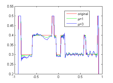
From figures 2 and 3, we can see that the presented algorithms can carry out the reconstruction of SPECT efficiently. As our expectation, the distortions in the reconstructions raise with the increase of the attenuation coefficient μ1\mu_{1}. The profiles of the reconstructions in figure 2 at x1=0x_{1}=0 are displayed in figure 4. Similar to [1], we have the same observation that the noise in the reconstructions appears strongly spatial variant, for which the reason is the weight variant in (3)(see [1] for details).
Refer to caption
Figure 4: Profiles of the images reconstructed from perfect non-truncated projection data in figure 2.

4 Conclusions and discussions

In this work, a numerical method for the CHT is presented. The numerical experiments show that the proposed method can conduct the SPECT reconstruction for practical attenuation constant approximately. On the other hand, we can observe that there are great distortions with the increasing of attenuation constant. Though numerical methods can inverse the CHT approximately, great efforts are needed to seek a analytic inversion formula and more robust numerical methods for larger attenuation constant μ1\mu_{1}.

Acknowledgements

This work is supported by the National Basic Research Program of China (2011CB809105) and NSF grants of China (61121002, 10990013). The authors are grateful for helpful discussions with Professor Haomin Zhou(School of Mathematics, Georgia Institute of Technology).

Appendix

In this appendix, we give the analytic formulae for the computation of Ti​(t)T_{i}(t) and TijT_{i}^{j}. And we will discuss the numerical method of did_{i}, which is very important for the accurate reconstruction.
Computation of Tn​(t)T_{n}(t): Firstly, we have [11]

T0​(t)\displaystyle T_{0}(t) =\displaystyle= 1π​∫−111−τ2t−τ​𝑑τ=t.\displaystyle{1\over\pi}\int_{-1}^{1}\frac{\sqrt{1-\tau^{2}}}{t-\tau}d\tau=t. (24)

By this result, we can compute Tn​(t)T_{n}(t)(n>0n>0) by recursive relationship

Tn​(s)\displaystyle T_{n}(s) =\displaystyle= 1π​∫−11tn​1−t2s−t​𝑑t\displaystyle{1\over\pi}\int_{-1}^{1}{t^{n}{\sqrt{1-t^{2}}}\over{s-t}}dt (25)
=\displaystyle= 1π​∫−11tn−1​s−(s−t)s−t​1−t2​𝑑t\displaystyle{1\over\pi}\int_{-1}^{1}t^{n-1}{{s-(s-t)}\over{s-t}}\sqrt{1-t^{2}}dt
=\displaystyle= 1π​∫−11tn−1​1s−t​1−t2​𝑑t−1π​∫−11tn−1​1−t2​𝑑t\displaystyle{1\over\pi}\int_{-1}^{1}t^{n-1}{{1}\over{s-t}}\sqrt{1-t^{2}}dt-{1\over\pi}\int_{-1}^{1}t^{n-1}\sqrt{1-t^{2}}dt
=\displaystyle= s​Tn−1​(s)−Sn−1,\displaystyle sT_{n-1}(s)-S_{n-1},

where Sn={0n​ is oddB2​n−B2​n+2n​ is even,S_{n}=\left\{\begin{array}[]{ll}0&n\textrm{ is odd}\\ B_{2n}-B_{2n+2}&n\textrm{ is even}\end{array}\right., and B2​n=1π​∫−π2π2sin2​n⁡(α)​𝑑α=(2​n−2)!!(2​n)!!B_{2n}={1\over\pi}\int_{-{\pi\over 2}}^{\pi\over 2}\sin^{2n}(\alpha)d\alpha=\frac{(2n-2)!!}{(2n)!!}.
Computation of Tij​(t)T_{i}^{j}(t): Firstly, we have that Tn​(−t)=(−1)n​T​(t)T_{n}(-t)=(-1)^{n}T(t) by the definition of Tn​(t)T_{n}(t). Therefore, we have T2​n2​k=0,T2​n+12​k+1=0T_{2n}^{2k}=0,T_{2n+1}^{2k+1}=0 for n,k≥0n,k\geq 0, and T02​k+1=(2​k+1)!!(2​k+2)!!=B2​k+2T_{0}^{2k+1}={{(2k+1)!!}\over{(2k+2)!!}}=B_{2k+2} because T0​(t)=tT_{0}(t)=t. By using the recursive formula (25) of Tn​(t)T_{n}(t), we have

T2​n2​k+1\displaystyle T_{2n}^{2k+1} =\displaystyle= 1π​∫−11s2​k+11−s2​T2​n​(s)​𝑑s\displaystyle{1\over\pi}\int_{-1}^{1}{{s^{2k+1}\over\sqrt{1-s^{2}}}T_{2n}(s)}ds (26)
=\displaystyle= 1π​∫−11s2​k+11−s2​(s​T2​n−1​(s))​𝑑s\displaystyle{1\over\pi}\int_{-1}^{1}{{s^{2k+1}\over\sqrt{1-s^{2}}}(sT_{2n-1}(s))}ds
=\displaystyle= T2​n−12​k+2,\displaystyle T_{2n-1}^{2k+2},

and

T2​n+12​k\displaystyle T_{2n+1}^{2k} =\displaystyle= 1π​∫−11s2​k1−s2​T2​n+1​(s)​𝑑s\displaystyle{1\over\pi}\int_{-1}^{1}{s^{2k}\over\sqrt{1-s^{2}}}T_{2n+1}(s)ds (27)
=\displaystyle= 1π​∫−11s2​k1−s2​(s​T2​n​(s)−S2​n)​𝑑s\displaystyle{1\over\pi}\int_{-1}^{1}{s^{2k}\over\sqrt{1-s^{2}}}(sT_{2n}(s)-S_{2n})ds
=\displaystyle= T2​n2​k+1−S2​n​B2​k.\displaystyle T_{2n}^{2k+1}-S_{2n}B_{2k}.

Computation of did_{i}: In order to get the unknown function f⁡(t)f(t) for |t|<1|t|<1 finally, we should divide 1−t2\sqrt{1-t^{2}} on both sides of (19), which implies that tiny errors near the two ends −1-1 and 1 must result in large deviations from f⁡(t)f(t). Therefore, we have to compute cic_{i} and did_{i} precisely to suppress the errors on two ends. Because the computation formula for each did_{i} can be seen as the 11−t2\frac{1}{\sqrt{1-t^{2}}} weighted integral of fμ1​(t)​tif_{\mu_{1}}(t)t^{i}, we use the Gauss-Chebyshev quadrature formula[12] in this paper.

1π​∫−11s⁡(t)1−t2​𝑑t≈πn​∑i=1ns⁡(qi),\displaystyle{1\over\pi}\int_{-1}^{1}\frac{s(t)}{\sqrt{1-t^{2}}}dt\approx{\pi\over n}\sum_{i=1}^{n}s(q_{i}), (28)

where the Gauss-Chebyshev nodes of (28) are given by qi=cos⁡2​i−12​n​πq_{i}=\cos{\frac{2i-1}{2n}\pi}.

References

  • [1] F. Noo, M. Defrise, J. D. Pack, and R. Clackdoyle, “Image reconstruction from truncated data in single-photon emission computed tomography with uniform attenuation,” Inverse Problems, vol. 23, no. 2, pp. 645–667, 2007.
  • [2] J. You, G. L. Zeng, and Q. Huang, “Finite inversion of the weighted hilbert transform - application to medical imaging,” in Proceedings of Meeting on Fully 3D Image Reconstruction in Radiology and Nuclear Medicine, Lindau, Germany.
  • [3] F. Natterer and F. Wübbeling, Mathematical Methods in Image Reconstruction. Philadelphia: Society for Industrial and Applied Mathematics, 2001.
  • [4] R. G. Novikov, “An inversion formula for the attenuated x-ray transformation,” vol. 40, pp. 145–167, 2002.
  • [5] F. Natterer, “Inversion of the attenuated radon transform,” Inverse Problems, vol. 17, pp. 113–119, 2001.
  • [6] O. Tretiak and C. Metz, “The exponential radon transform,” SIAM Journal on Applied Mathematics, vol. 39, pp. 341–54, 1980.
  • [7] F. Noo and J.-M. Wagner, “Image reconstruction in 2d spect with 180∘ acquisition,” Inverse Problems, vol. 17, pp. 1357–1371, 2001.
  • [8] “A family of π\pi-scheme exponential radon transforms and the uniqueness of their inverses,” vol. 18, pp. 825–836, 2002.
  • [9] H. Rullgård, “An explicit inversion formula for the exponential radon transform using data from 180∘,” Ark. Mat., vol. 42, pp. 353–362, 2004.
  • [10] Q. Huang, J. You, G. L. Zeng, and G. T. Gullberg, “Exact reconstruction from uniformly attenuated helical cone-beam projections in spect,” escholar, 2009.
  • [11] F. G. Tricomi, Integral Equations. New York: Interscience Springer, 1957.
  • [12] H. Engels, Numerical quadrature and cubature. New York: Academic Press, 1980.