Higgs boson production in association with a jet at next-to-next-to-leading order in perturbative QCD

Preprint: ANL-HEP-PR-13-13

Radja Boughezal Affiliation: High Energy Physics Division, Argonne National Laboratory, Argonne, IL 60439, USA Email: rboughezal@anl.gov Fabrizio Caola Affiliation: Department of Physics and Astronomy, Johns Hopkins University, Baltimore, MD 21218, USA Email: caola@pha.jhu.edu Kirill Melnikov Affiliation: Department of Physics and Astronomy, Johns Hopkins University, Baltimore, MD 21218, USA Email: melnikov@pha.jhu.edu Frank Petriello Affiliation: High Energy Physics Division, Argonne National Laboratory, Argonne, IL 60439, USA Affiliation: Department of Physics & Astronomy, Northwestern University, Evanston, IL 60208, USA Email: f-petriello@northwestern.edu and Markus Schulze Affiliation: High Energy Physics Division, Argonne National Laboratory, Argonne, IL 60439, USA Email: markus.schulze@anl.gov

Abstract

We report on a calculation of the cross-section for Higgs boson production in gluon fusion in association with a hadronic jet at next-to-next-to-leading order (NNLO) in perturbative QCD. The computational technique is discussed in detail. We show explicitly how to employ known soft and collinear limits of scattering amplitudes to construct subtraction terms for NNLO computations. Cancellation of singularities is demonstrated numerically for the collinearly-subtracted $gg\to H+j$ cross-section through NNLO and the finite $\sigma_{gg\to Hj}$ cross-section is computed through ${\cal O}(\alpha_{s}^{5})$ as a function of the center-of-mass collision energy. We present numerical results for the gluon-fusion contribution to Higgs production in association with a jet at the LHC. The NNLO QCD corrections significantly reduce the residual scale dependence of the cross-section. The computational method that we describe in this paper is applicable to the calculation of NNLO QCD corrections to any other $2\to 2$ process at a hadron collider without modification.

1 Introduction

The ATLAS and CMS experiments at the Large Hadron Collider (LHC) have discovered a new particle with a mass of approximately $125~{\rm GeV}$ [1, 2] whose properties are consistent with that of the Standard Model Higgs boson. Continuing studies at the LHC are focusing on the detailed understanding of the quantum numbers of this particle [3] and its couplings to gauge bosons and fermions (see e.g. [4] and references therein). The successful completion of this task is crucial for determining if the new particle is indeed the long-awaited Higgs boson or instead some other state.

A reliable understanding of coupling constants cannot occur without accurate theoretical predictions for the main Higgs boson production and decay processes. Arriving at such predictions requires the computation of higher-order QCD corrections, since they are known to affect Higgs production rates and decay branching fractions in a significant way. In fact, for gluon-initiated processes $gg\to H+X$ , where $X$ is a state with zero, one or two hard jets, the next-to-leading order (NLO) QCD radiative corrections are known to be so large [5, 6, 7, 8, 9, 10, 11, 12] that next-to-next-to-leading order (NNLO) QCD computations are important for reliable phenomenology.

Unfortunately, current computational technology only allows NNLO QCD computations for the case of Higgs boson production in association with zero jets [13, 14, 15, 16, 17]. Extending this result to one or more jets will lead to a refined analysis of the $pp\to H\to W^{+}W^{-}$ process, since in that case final states with different jet multiplicities are treated as different processes in order to optimize search strategies. The information about the relative significance of the Higgs boson production in association with zero, one or two jets is currently extracted from available fixed-order computations supplemented with resummations of the most important terms in the perturbative expansion [18, 19, 20, 21]. Explicit NNLO computations for multi-jet processes will be indispensable for understanding the reliability of these predictions.

The other motivation for this work is of a more theoretical nature. One can argue that the framework of perturbative QCD that has been developed since the late 1970’s has proven to be one of the most important areas of particle physics phenomenology. Indeed, it is impossible to imagine contemporary high-energy physics without hadron collider physics whose proper description is intimately related with parton shower event generators, sophisticated fits of parton distribution functions, fixed-order perturbative calculations and the like. Much of our understanding of perturbative QCD is based on how soft and collinear singularities cancel in suitable “infra-red safe” quantities, since this defines short-distance observables that can be calculated in perturbation theory. Currently, there exists an interesting gap in this understanding. On one hand, general theorems [22, 23] ensure that this cancellation occurs in suitably defined quantities to all orders in perturbation theory. On the other hand, we only know how to use those ideas for generic computations of infra-red-safe observables at leading and next-to-leading order in perturbative QCD [24, 25]. It is still not entirely clear how to construct a general calculational scheme for two- and higher-loop computations.

It is important to point out that, in spite of the fact that a generic computational scheme is not available, a fairly large number of NNLO computations for various processes have already been performed [17, 26, 27, 28, 29, 16, 30, 31, 32, 33, 34, 35, 36, 37, 38, 39], but until very recently such computations always utilized a particular aspect of a specific process. Such aspects included a small number of final-state particles, or their color neutrality, or absence of color-charged particles in the initial state, or even the fact that all matter particles in a particular process were massive. A generic algorithm that is valid irrespective of the details of the process under consideration was not worked out. This situation is somewhat peculiar, because following the successful development of generic methods for NLO computations [24, 25], it was generally felt that the development of similar methods for NNLO computations would be relatively straightforward. For this reason, about ten years ago many authors calculated infra-red and collinear limits of generic QCD amplitudes [40, 41, 42, 43, 44, 45, 46, 47] that are potentially relevant for NNLO computations, and a large number of two-loop $2\to 2$ scattering amplitudes became available [48, 49]. Unfortunately, since it proved harder than expected to develop a working scheme for NNLO computations, these infra-red and collinear limits were never used for their intended purpose.

Recently, important steps towards developing a general computational scheme valid through NNLO QCD that, at least in principle, is applicable to processes of arbitrary multiplicity, were made by Czakon [55, 56], who suggested to combine the ideas of sector decomposition [57, 58, 59] and Frixione-Kunszt-Signer (FKS) [25] phase-space partitioning. These results were used to obtain NNLO QCD corrections to the cross-sections for $q\bar{q}\to t\bar{t}$ [60, 61] and $qg\to t\bar{t}$ [62] processes. A similar computational scheme was also developed in Ref. [63] where it was applied to the calculation of NNLO QED corrections to $Z\to e^{+}e^{-}$ . We note that parallel developments in the antennae subtraction technique [64] have recently led to the calculation of the NNLO QCD corrections to the leading-color all-gluon contribution to di-jet production at the LHC [65].

While the above results mark important progress in developing a suitable framework for NNLO computations, a large number of technical aspects still needs to be understood and worked out. It is best to do this by considering a realistic example with all the ensuing complications. This is the purpose of the current paper. We consider the hadro-production of the Higgs boson in association with one hadronic jet at NNLO in QCD. To make calculations as simple as possible, we work in pure gluodynamics, i.e. QCD without light fermions. We note that an understanding of how to compute the NNLO QCD corrections to $H+j$ production is instructive because this process possesses all non-trivial aspects of a generic NNLO QCD problem. Indeed,

•

there are colored particles in the initial state;
•

there are colored particles in the final state;
•

already at leading order, the total cross-section for this process does not exist unless a jet algorithm is specified;
•

this process exhibits the most general structure of infra-red and collinear singularities, since these singularities occur due to radiation of gluons in the initial and final states;
•

singular collinear splittings $g\to gg$ involve non-trivial spin correlations;
•

the number of Feynman diagrams that we need to compute is large.¹¹ 1 For example, the process $gg\to Hggg$ is described at leading order by 230 diagrams while the $gg\to Hgg$ process at one-loop is described by 603 diagrams.

The only “non-generic” feature of the process that we consider is the high symmetry of the final state which simplifies the bookkeeping and speeds up the computation. We feel, however, that having this simplification is useful in the first step in the development of the new technology and that it does not affect the generality of the method that we describe in this paper.

The remainder of the paper is organized as follows. In the next Section we describe the setup of the calculation. In Section 3 we discuss the parametrizations of the phase-space for leading, next-to-leading and next-to-next-to-leading order computations. In Section 4 we explain how singular limits of amplitudes are used. In Section 5 we describe how ${\cal O}(\epsilon)$ parts of the relevant amplitudes can be computed using helicity methods. In Section 6 we describe the numerical implementation of our method. In Section 7 we discuss some tests and show the results of the computation. We conclude in Section 8. Some useful formulae are given in the Appendix.

2 The setup

We are interested in the computation of NNLO QCD corrections to the process $g+g\to H+g$ , where the Higgs boson can decay into arbitrary particles. To compute this and related processes, we use the QCD Lagrangian, supplemented with a dimension-five non-renormalizable operator that describes the interaction of the Higgs boson with gluons in the limit of very large top quark mass

{\cal L}=-\frac{1}{4}G_{\mu\nu}^{(a)}G^{(a),\mu,\nu}-\lambda_{Hgg}HG_{\mu\nu}^{(a)}G^{(a),\mu,\nu}.

(1)

Here, $G_{\mu\nu}^{(a)}$ is the field-strength tensor of the gluon field and $H$ is the Higgs boson field.

Matrix elements computed with the Lagrangian of Eq. (1) need to be renormalized; to do so, two renormalization constants are required. The first one relates bare and renormalized QCD coupling constants

\alpha_{s}^{(0)}\mu_{0}^{2\epsilon}S_{\epsilon}=\mu^{2\epsilon}\alpha_{s}Z_{\alpha_{s}},\;\;\ Z_{\alpha_{s}}=1-\frac{\beta_{0}}{\epsilon}\left(\frac{\alpha_{s}}{2\pi}\right)+\left(\frac{\beta_{0}^{2}}{\epsilon^{2}}-\frac{\beta_{1}}{2\epsilon}\right)\left(\frac{\alpha_{s}}{2\pi}\right)^{2}+....

(2)

Here, $\alpha_{s}$ is the strong coupling constant in the ${\overline{\rm MS}}$ scheme evaluated at the renormalization scale $\mu$ , $S_{\epsilon}=(4\pi)^{-\epsilon}e^{-\gamma\epsilon},\;\gamma=0.5772$ is the Euler constant and

\beta_{0}=\frac{11N_{c}}{6},\;\;\;\;\;\;\;\beta_{1}=\frac{17N_{c}^{2}}{6}

(3)

are one- and two-loop contributions to the QCD $\beta$ -function computed with the Lagrangian of Eq. (1). $N_{c}=3$ is the number of colors. We note that Eq. (3) is only valid in a theory without light fermions, as defined by the Lagrangian Eq. (1).

The second renormalization constant ensures that matrix elements of the $HGG$ dimension-five operator are finite. It reads

\lambda_{Hgg}^{(0)}=-\frac{\alpha_{s}}{12\pi v}C(\alpha_{s})Z_{\rm eff}(\alpha_{s}),\;\;\;\ Z_{\rm eff}=1-\frac{\beta_{0}}{\epsilon}\left(\frac{\alpha_{s}}{2\pi}\right)+\left(\frac{\beta_{0}^{2}}{\epsilon^{2}}-\frac{\beta_{1}}{\epsilon}\right)\left(\frac{\alpha_{s}}{2\pi}\right)^{2}+..

(4)

In the above formula, $C(\alpha_{s})$ is the Wilson coefficient of the $HGG$ operator in the ${\overline{\rm MS}}$ scheme [51]

C=1+\frac{11}{2}\left(\frac{\alpha_{s}}{2\pi}\right)+\left(\frac{\alpha_{s}}{2\pi}\right)^{2}\left[\frac{2777}{72}+\frac{19}{4}\ln\frac{\mu^{2}}{m_{t}^{2}}\right]+{\cal O}(\alpha_{s},N_{f}),

(5)

where $m_{t}$ is the mass of the top quark. We emphasize again that the displayed result is only valid in the approximation when no light fermions are present in the theory.

Renormalization of the strong coupling constant and of the effective Higgs-gluon coupling removes ultraviolet divergences from the matrix elements. The remaining divergences are of infra-red origin. To remove them, we must both define and compute infra-red safe observables, and absorb remaining collinear singularities by renormalizing parton distribution functions. We now discuss these two issues.

Generic infra-red safe observables are defined using jet algorithms. For the calculation described in this paper we employ the $k_{\perp}$ -algorithm. This algorithm belongs to the class of sequential jet algorithms. It requires specification of the minimal transverse momentum of the reconstructed jets $p_{\perp,j}$ and the minimal “angular” distance between two partons, $\Delta R_{\penalty\hskip 0.0pti\kern-0.16391pt\penalty\hskip 0.0ptj}=\sqrt{(y_{i}-y_{j})^{2}+(\varphi_{i}-\varphi_{j})^{2}}$ , where $y=1/2\ln(E+p_{z})/(E-p_{z})$ is the rapidity and $\varphi$ is the azimuthal angle of a parton. Once $\Delta R$ and $p_{\perp,j}$ are specified, the jet algorithm maps a set of parton momenta onto a set of jet momenta in such a way that jet momenta are stable against soft and collinear parton splittings. The Kinoshita-Lee-Naunberg theorem [22, 23] then ensures that observables constructed from jet four-momenta are determined by short-distance physics and can therefore be computed in QCD perturbation theory. However, because massless colored partons are present in the initial state of the partonic process $gg\to H+X$ , the infra-red and collinear cancellation is not complete, even in the presence of a jet algorithm. Collinear singularities associated with gluon radiation by incoming partons must be removed by additional renormalization of parton distribution functions. We describe how to perform this renormalization in what follows. For definiteness, we focus our discussion on the production cross-section of a Higgs boson and a jet in pure gluodynamics.

We denote the UV-renormalized partonic cross-section for the production of the Higgs boson and a jet in a gluon fusion by ${\bar{\sigma}}(x_{1},x_{2})$ , and the collinear-renormalized partonic cross-section by $\sigma(x_{1},x_{2})$ . Once we know $\sigma(x_{1},x_{2})$ , we can compute the hadronic cross-sections by integrating the product of $\sigma$ and gluon distribution functions over $x_{1}$ and $x_{2}$

\sigma(p+p\to H+j)=\int{\rm d}x_{1}{\rm d}x_{2}\;g(x_{1})g(x_{2})\;\sigma(x_{1},x_{2}).

(6)

The relation between $\sigma$ and ${\bar{\sigma}}$ is given by the following formula ²² 2 We show this relation for pure gluodynamics; if more species of partons are present, Eq. (7) becomes a matrix equation.

\sigma=\Gamma^{-1}\otimes{\bar{\sigma}}\otimes\Gamma^{-1},

(7)

where the convolution sign stands for

\left[f\otimes g\right](x)=\int\limits_{0}^{1}{\rm d}x{\rm d}y\delta(x-yz)f(y)g(z).

(8)

The collinear counter-terms are defined as

\Gamma=\delta(1-x)-\left(\frac{\alpha_{s}}{2\pi}\right)\Gamma_{1}+\left(\frac{\alpha_{s}}{2\pi}\right)^{2}\Gamma_{2},

(9)

with

\Gamma_{1}=\frac{P_{gg}^{(0)}}{\epsilon},\;\;\;\;\Gamma_{2}=\frac{1}{2\epsilon^{2}}\left(P_{gg}^{(0)}\otimes P_{gg}^{(0)}+\beta_{0}P^{(0)}_{gg}\right)-\frac{1}{2\epsilon}P_{gg}^{(1)}.

(10)

The relevant splitting functions and their convolutions are given in the Appendix. We write the UV-renormalized partonic cross-section through NNLO as

{\bar{\sigma}}={\bar{\sigma}}^{(0)}+\left(\frac{\Gamma(1+\epsilon)\alpha_{s}}{2\pi}\right){\bar{\sigma}}^{(1)}+\left(\frac{\Gamma(1+\epsilon)\alpha_{s}}{2\pi}\right)^{2}{\bar{\sigma}}^{(2)},

(11)

and the collinear-renormalized partonic cross-section as

\sigma=\sigma^{(0)}+\left(\frac{\alpha_{s}}{2\pi}\right){\sigma}^{(1)}+\left(\frac{\alpha_{s}}{2\pi}\right)^{2}{\sigma}^{(2)}.

(12)

We note that the collinear-renormalized cross-section is finite. We then use Eq. (7) to obtain

\begin{split}&\sigma^{(0)}={\bar{\sigma}}^{(0)},\;\;\;\;\;\;\;\;\;\;\;\sigma^{(1)}={\bar{\sigma}}^{(1)}+\frac{\Gamma_{1}\otimes{\sigma}^{(0)}}{\Gamma(1+\epsilon)}+\frac{{\sigma}^{(0)}\otimes\Gamma_{1}}{\Gamma(1+\epsilon)},\\ &\sigma^{(2)}={\bar{\sigma}}^{(2)}-\frac{\Gamma_{2}\otimes{\sigma}^{(0)}}{\Gamma(1+\epsilon)^{2}}-\frac{{\sigma}^{(0)}\otimes\Gamma_{2}}{\Gamma(1+\epsilon)^{2}}-\frac{\Gamma_{1}\otimes{\sigma}^{(0)}\otimes\Gamma_{1}}{\Gamma(1+\epsilon)^{2}}+\frac{\Gamma_{1}\otimes\sigma^{(1)}}{\Gamma(1+\epsilon)}+\frac{\sigma^{(1)}\otimes\Gamma_{1}}{\Gamma(1+\epsilon)}.\end{split}

(13)

Although finite, the $\sigma^{(i)}$ still depend on unphysical renormalization and factorization scales because of the truncation of the perturbative expansion. In the following, we will consider for simplicity the case of equal renormalization and factorization scales , $\mu_{r}=\mu_{f}=\mu$ . The residual $\mu$ dependence is easily determined by solving the renormalization group equation order-by-order in $\alpha_{s}$ . The equation reads

0=\mu^{2}\frac{{\rm d}\sigma_{p+p\to H+j}}{{\rm d}\mu^{2}}=\mu^{2}\frac{\rm d}{{\rm d}\mu^{2}}\int{\rm d}x_{1}{\rm d}x_{2}g(x_{1},\mu^{2})g(x_{2},\mu^{2})\sigma(x_{1},x_{2},\alpha_{s}(\mu^{2}),\mu^{2}).

(14)

The $\mu$ -derivative of the right hand side can be computed using the known evolution equations for the strong coupling constant and the gluon density

\begin{split}&\mu^{2}\frac{\partial\alpha_{s}}{\partial\mu^{2}}=-\alpha_{s}\left(\beta_{0}\frac{\alpha_{s}}{2\pi}+\beta_{1}\left(\frac{\alpha_{s}}{2\pi}\right)^{2}+\mathcal{O}(\alpha_{s}^{3})\right),\\ &\mu^{2}\frac{\partial g(\mu^{2})}{\partial\mu^{2}}=\frac{\alpha_{s}}{2\pi}\;g(\mu^{2})\otimes\left(P_{gg}^{(0)}+\frac{\alpha_{s}}{2\pi}P_{gg}^{(1)}+\mathcal{O}(\alpha_{s}^{2})\right).\end{split}

(15)

Solving these renormalization group equations, we get

\begin{split}\sigma^{(0)}_{\mu_{1}}&=\sigma^{(0)}_{\mu_{2}},\;\;\;\;\;\;\;\sigma^{(1)}_{\mu_{1}}=\sigma^{(1)}_{\mu_{2}}+L_{12}\left(3\beta_{0}\sigma^{(0)}_{\mu_{2}}-P_{gg}^{(0)}\otimes\sigma^{(0)}_{\mu_{2}}-\sigma^{(0)}_{\mu_{2}}\otimes P_{gg}^{(0)}\right),\\ \sigma^{(2)}_{\mu_{1}}&=\sigma^{(2)}_{\mu_{2}}+L_{12}\left(4\beta_{0}\sigma_{\mu_{2}}^{(1)}-P_{gg}^{(0)}\otimes\sigma^{(1)}_{\mu_{2}}-\sigma^{(1)}_{\mu_{2}}\otimes P_{gg}^{(0)}+3\beta_{1}\sigma_{\mu_{2}}^{(0)}-P_{gg}^{(1)}\otimes\sigma^{(0)}_{\mu_{2}}+\right.\\ &-\left.\sigma^{(0)}_{\mu_{2}}\otimes P_{gg}^{(1)}\right)+\frac{1}{2}L_{12}^{2}\left(12\beta_{0}^{2}\sigma_{\mu_{2}}^{(0)}-7\beta_{0}\left(P_{gg}^{(0)}\otimes\sigma^{(0)}_{\mu_{2}}+\sigma^{(0)}_{\mu_{2}}\otimes P_{gg}^{(0)}\right)+\right.\\ &+\left.P_{gg}^{(0)}\otimes P_{gg}^{(0)}\otimes\sigma_{\mu_{2}}^{(0)}+\sigma_{\mu_{2}}^{(0)}\otimes P_{gg}^{(0)}\otimes P_{gg}^{(0)}+2P_{gg}^{(0)}\otimes\sigma_{\mu_{2}}^{(0)}\otimes P_{gg}^{(0)}\right),\end{split}

(16)

where $\sigma_{\mu}^{(i)}\equiv\sigma^{(i)}(\alpha_{s}(\mu),\mu)$ and $L_{12}=\ln\mu_{1}^{2}/\mu_{2}^{2}$ .

It follows from Eqs. (13,16) that, in order to obtain $\sigma^{(2)}$ at a generic scale, apart from lower-order results we need to know the NNLO renormalized cross-section ${\bar{\sigma}}^{(2)}$ and convolutions of NLO and LO cross-sections with various splitting functions. Up to terms induced by the renormalization, there are three contributions to ${\bar{\sigma}}^{(2)}$ that are required:

•

the two-loop virtual corrections to $gg\to Hg$ ;
•

the one-loop virtual corrections to $gg\to H+gg$ ;
•

the double-real contribution $gg\to H+ggg$ .

We note that helicity amplitudes for all of these processes are available in the literature. The two-loop amplitudes for $gg\to Hg$ were recently computed in Ref. [50]. The one-loop corrections to $gg\to Hgg$ [52] and the tree amplitudes for $gg\to Hggg$ [53] are known. Moreover, in the two latter cases, these amplitudes are available in the form of a Fortran code in the program MCFM [66]. In principle, they can be just taken from MCFM and used with no modification in another numerical program.

Since the above discussion implies that all ingredients for the NNLO computation of $gg\to H+{\rm jet}$ are available and, in fact, have been available for some time, it is important to understand what has prevented the community from performing this and similar calculations. In fact, the main difficulties with NNLO calculations appear when we attempt to combine the different contributions, since integration over phase-space introduces additional singularities if the required number of jets is lower than the parton multiplicity. To perform the phase-space integration, we must first isolate singularities in tree- and loop amplitudes. It required a long time to establish a convenient way to do this.

The computational method that we will explain shortly is based on the idea that relevant singularities can be isolated using appropriate parametrizations of phase-space and expansions in plus-distributions [25, 59]. To illustrate this point, we consider the integral

I(\epsilon)=\int\limits_{0}^{1}{\rm d}xx^{-1-a\epsilon}F(x),

(17)

where the function $F(x)$ has a well-defined limit $\lim\limits_{x\to 0}F(x)=F(0)$ . We would like to construct the Laurent expansion of $I$ in $\epsilon$ . This can be accomplished by writing

\frac{1}{x^{1+a\epsilon}}=-\frac{1}{a\epsilon}\delta(x)+\sum_{n=0}^{\infty}\frac{(-\epsilon a)^{n}}{n!}\left[\frac{\ln^{n}(x)}{x}\right]_{+}

(18)

so that

I(\epsilon)=\int\limits_{0}^{1}{\rm d}x\left(-\frac{F(0)}{a\epsilon}+\frac{F(x)-F(0)}{x}-a\epsilon\frac{F(x)-F(0)}{x}\ln(x)+...\right).

(19)

The above equation provides the required Laurent expansion of the integral $I(\epsilon)$ . We note that each term in such an expansion can be calculated independently from other terms.

To use this approach for computing NNLO QCD corrections, we need to map the relevant phase-space to a unit hypercube in such a way that extraction of singularities is straightforward. It is intuitively clear that correct variables to use are the re-scaled energies of unresolved partons and the relative angles between two unresolved (collinear) partons. However, the problem is that different partons become unresolved in different parts of the phase-space. It is not immediately clear how to switch between different sets of coordinates and cover the full phase-space.

We note that for NLO QCD computations, this problem was solved in Ref. [25], where it was explained that the full phase-space can be partitioned into sectors in such a way that in each sector only one parton ( $i$ ) can produce a soft singularity and only one pair of partons ( $ij$ ) can produce a collinear singularity. In each sector, the proper variables are the energy of the parton $i$ and the relative angle between partons $i$ and $j$ . Once the partitioning of the phase-space is established and proper variables are chosen for each sector, we can use an expansion in plus-distributions to construct relevant subtraction terms for each sector. With the subtraction terms in place, the Laurent expansion of cross-sections in $\epsilon$ can be constructed, and each term in such an expansion can be integrated over the phase-space independently. Therefore, partitioning of the phase-space into suitable sectors and proper parametrization of the phase-space in each of these sectors are the two crucial elements needed to extend this method to NNLO. In the next Section we discuss these issues in detail.

3 Phase-space parametrizations and sector decomposition

3.1 Phase-space for leading order processes

We now discuss how to parametrize the leading-order phase-space for the process $g_{1}+g_{2}\to H+g_{3}$ . This will be needed both for the leading-order cross section and for the NLO virtual and NNLO double virtual corrections, so it must be computed in $d=4-2\epsilon$ dimensions. We note that the integration over the leading order phase-space is not singular, because of the requirement that a jet is observed. We work in the center-of-mass frame of the two incoming gluons, so that their momenta are parametrized as

p_{1}=\frac{\sqrt{s}}{2}\left(1,0,0,1\right),\;\;\;\;p_{2}=\frac{\sqrt{s}}{2}\left(1,0,0,-1\right).

(20)

The center-of-mass collision energy is denoted by $\sqrt{s}$ and the mass of the Higgs boson is denoted by $m_{H}$ . The production cross-section, averaged over spins and colors of the two colliding gluons, is written as

{\rm d}{\rm\sigma}_{gg\to H+g}=\frac{1}{512s}{\rm d}{\rm Lips}_{12\to H3}|{\cal M}_{gg\to gH}|^{2}\times F_{j},

(21)

where $F_{j}$ is the “measurement function” that restricts the integration to the region of phase-space where there is an identified jet. The amplitude ${\cal M}_{gg\to gH}$ describes production of an on-shell Higgs boson in hadronic collisions and ${\rm d}{\rm Lips}_{12\to H3}$ is the Lorentz-invariant phase-space.

The parametrization of the phase-space ${\rm d}{\rm Lips}_{12\to 3H}$ in Eq. (21) is easily obtained by integrating over the momentum of the on-shell Higgs boson and then over the center-of-mass energy of the gluon $g_{3}$ . We find

{\rm d}{\rm Lips}_{12\to 3H}=\frac{{\rm d}\Omega^{(d-2)}_{3}p_{\perp,H}^{-2\epsilon}\;{\rm d}\cos\theta_{3}}{8(2\pi)^{d-2}}\left(1-\frac{m_{H}^{2}}{s}\right),\;\;\;\;\;p_{\perp,H}=E_{\rm max}\sin\theta_{3},

(22)

where $E_{\rm max}=(s-m_{H}^{2})/(2\sqrt{s})$ . With this parametrization, the momentum of the gluon $g_{3}$ reads

p_{3}=E_{\rm max}\left(1,\vec{n}_{3}\right),

(23)

where $n_{3}=\left(\sin\theta_{3}\cos\varphi_{3},\sin\theta_{3}\sin\varphi_{3},\cos\theta_{3}\right)$ , and the Higgs boson momentum is obtained from momentum conservation: $p_{H}=p_{1}+p_{2}-p_{3}$ . Note that in Eq. (22), $p_{\perp,H}$ is the transverse momentum of the Higgs boson relative to the collision axis.

Before proceeding further, we note that the azimuthal angle $\varphi_{3}$ of the emitted gluon is a dummy variable, since neither matrix element squared nor the measurement function $F_{J}$ depend on it for our choice of $p_{1}$ and $p_{2}$ . Hence, we can rotate it away by taking the $g_{3}$ momentum to be

p_{3}=E_{\rm max}\left(1,\sin\theta_{3},0,\cos\theta_{3}\right),

(24)

and integrate over ${\rm d}\Omega^{(d-2)}_{3}$ in Eq. (22). Once this is done, we can set this solid angle to its four-dimensional expression to simplify calculations at higher orders. This is legitimate to do as long as we can identify this angle, associated with global rotations of final states in the plane transverse to the collision axis, when parametrizing higher-multiplicity phase-spaces. Nevertheless, to maintain sufficiently general leading order kinematics, we re-introduce the azimuthal angle $\varphi_{3}$ and keep it to generate momenta of the gluon and the Higgs boson. This amounts to writing ${\rm d}\Omega^{(d-2)}_{3}\to{\rm d}\varphi_{3}$ in Eq. (22) and then using Eq. (23) for the gluon $g_{3}$ momentum. In addition, since the transverse momentum of the Higgs boson is an observable quantity, the differential cross-section ${\rm d}\sigma/{\rm d}p_{\perp,H}$ should be finite for each value of $p_{\perp,H}$ to all orders in perturbation theory. Hence, we can divide the cross-section by $p_{\perp,H}^{-2\epsilon}$ without changing the final result. This amounts to removing this factor from the phase-space parametrization at both leading and higher orders in perturbation theory. Putting all these remarks together, we conclude that we can choose the leading order phase-space to be “four-dimensional,”

{\rm d}{\rm Lips}_{12\to 3H}\to\frac{{\rm d}\cos\theta_{3}{\rm d}\varphi_{3}}{32\pi^{2}}\left(1-\frac{m_{H}^{2}}{s}\right)=\left(1-\frac{m_{H}^{2}}{s}\right)\frac{{\rm d}x_{3}{\rm d}x_{4}}{8\pi},

(25)

where we introduced $\cos\theta_{3}=1-2x_{3}$ and $\varphi_{3}=2\pi x_{4}$ to parametrize the momentum of gluon $g_{3}$ as given by Eq. (23). We must remember to normalize NLO and NNLO phase-spaces to $p_{\perp,H}^{-2\epsilon}$ for consistency.

Although we will not discuss this in any detail in this paper, we note that it is straightforward to include decays of the Higgs boson. Indeed, because the Higgs boson momentum is an observable quantity, all singularities should cancel out in the differential cross-section ${\rm d}\sigma/{\rm d}\vec{p}_{H}$ . Once this differential cross-section is known and because the Higgs boson is a scalar particle, so that no spin correlations are present, we can easily turn ${\rm d}\sigma/{\rm d}\vec{p}_{H}$ into quantities such as ${\rm d}\sigma/{\rm d}\vec{p}_{\gamma_{1}}{\rm d}\vec{p}_{\gamma_{2}}$ by letting the Higgs boson decay in its rest frame and then boosting the four-momenta of the two photons into the center-of-mass frame.

3.2 Phase-space for next-to-leading order processes

In this Section, we consider the parametrization of the phase-space for the process $g_{1}+g_{2}\to H+g_{3}+g_{4}$ . This process represents a real-emission contribution to the production cross-section of the Higgs and one jet at next-to-leading order. It is also important for the NNLO computation where integration of one-loop corrections to $gg\to Hgg$ amplitudes over the $ggH$ phase-space is required.

As we already explained in the Introduction, a good parametrization of the phase-space ${\rm dLips}_{g_{1}g_{2}\to Hg_{3}g_{4}}$ should facilitate the extraction of singularities from the matrix elements of the process $g_{1}g_{2}\to Hg_{3}g_{4}$ . Of particular importance are collinear singularities. We can compare two cases: i) $g_{4}$ is emitted collinear to $g_{1}$ ; ii) $g_{4}$ is emitted collinear to $g_{3}$ . In the first case, it is easiest to extract the singularity if the $z$ -axis is chosen to coincide with the direction of the gluon $g_{1}$ and in the second case with the direction of the gluon $g_{3}$ . This immediately tells us that a suitable parametrization of the phase-space should depend on the kinematics of the process. As we mentioned in the Introduction, this is the main idea behind the FKS subtraction method [25].

Following Ref. [25], we note that the first step towards a convenient phase-space parametrization is the phase-space partitioning. The goal of such a partitioning is to create sectors where one and only one gluon or one and only one pair of gluons can become unresolved. Once we know which gluon or which pair of gluons can produce singularities, we choose the energy of the potentially soft gluon and the relative angle between the two potentially collinear gluons as the primary variables for the phase-space parametrization in the given sector. To illustrate this procedure, we begin by removing the symmetry between the two gluons in the final state by separating them into “resolved” and “unresolved” ones. To this end, we introduce the following function of transverse momenta of gluons $g_{3}$ and $g_{4}$ ,

\Delta^{(i)}_{p_{\perp}}=\frac{p_{\perp,j}}{p_{\perp,3}+p_{\perp,4}},\;\;\;j\neq i,

(26)

and write

\frac{1}{2!}{\rm d}{\rm Lips}_{12\to 34H}=\frac{1}{2!}{\rm d}{\rm Lips}_{12\to 34H}\left(\Delta_{p_{\perp}}^{(4)}+\Delta_{p_{\perp}}^{(3)}\right)\to{\rm d}{\rm Lips}_{12\to 34H}\Delta_{p_{\perp}}^{(4)}.

(27)

In the last step we used the fact that the phase space, the kinematic constraints on final-state particles and all matrix elements are symmetric with respect to permutations of gluons $g_{3}$ and $g_{4}$ . Given the structure of the damping factor $\Delta_{p_{\perp}}^{(4)}$ , it is clear that singularities of the matrix element related to gluon $g_{3}$ are unimportant, and we only need to consider cases when gluon $g_{4}$ becomes either soft or collinear to one of the three hard directions defined by the momenta $g_{1},g_{2}$ and $g_{3}$ . Note that $g_{3}$ and $g_{4}$ cannot both be soft, or collinear to the collision axis at the same time, because we require a jet in the final state. To separate the collinear-singular regions, we introduce another partition of unity

1=\Delta_{\theta}^{(41)}+\Delta_{\theta}^{(42)}+\Delta_{\theta}^{(43)}.

(28)

In Eq. (28), we use

\Delta_{\theta}^{(4i)}=\frac{\rho^{j4}\rho^{k4}}{\rho^{14}\rho^{24}+\rho^{14}\rho^{34}+\rho^{24}\rho^{34}},\;\;\;\;\;j,k\neq i,4,

(29)

where $\rho^{ij}=1-\vec{n}_{i}\cdot\vec{n}_{j}$ and $\vec{n}_{i}$ is the three-vector that parametrizes momentum direction of the particle $i$ . Again, the $\Delta_{\theta}^{(4i)}$ are labeled in such a way that the subscript indicates a pair of particles that can become collinear without forcing the angular damping factor to vanish. Inserting this partition of unity Eq. (28) into the phase-space of Eq. (27), we obtain

\frac{1}{2!}{\rm d}{\rm Lips}_{12\to 34H}\to\sum\limits_{i=1}^{3}{\rm d}{\rm Lips}_{12\to 34H}^{(4i)},\;\;\;\;{\rm d}{\rm Lips}_{12\to 34H}^{(4i)}={\rm d}{\rm Lips}_{12\to 34H}\Delta_{p_{\perp}}^{(4)}\Delta_{\theta}^{(4i)}.

(30)

The above decomposition defines pre-sectors that we will refer to as ${\rm Sc}^{(4i)}$ . A phase-space parametrization for each of these pre-sectors is chosen in such a way that the soft and collinear singularities that are relevant for that pre-sector can be extracted in the easiest possible way.

We now describe these parametrizations explicitly. In general, we will parametrize the phase-spaces by splitting them into “regular” and “singular” parts

{\rm d}{\rm Lips}_{12\to 34H}^{(4i)}=\Delta_{p_{\perp}}^{(4)}\Delta_{\theta}^{(4i)}{\rm d}{\rm Lips}_{Q(12)\to 3H}\times[{\rm d}g_{4}]^{(4i)}.

(31)

The regular NLO phase-space is the same for all pre-sectors. It includes all particles except the (potentially soft) gluon $g_{4}$ . We write it as

{\rm d}{\rm Lips}_{Q(12)\to 3H}=\frac{{\rm d}x_{4}{\rm d}x_{5}}{(8\pi)}\frac{2E_{g_{3}}}{(Q_{0}-\vec{Q}\cdot\vec{n}_{3})}\left(\frac{E_{g_{3}}^{2}\sin^{2}\theta_{3}}{p_{\perp,H}^{2}}\right)^{-\epsilon},

(32)

where we have introduced the notation $Q=p_{1}+p_{2}-p_{4}$ and $p_{3}=E_{g_{3}}(1,\vec{n}_{3})$ . Also,

\begin{split}&E_{g_{3}}=\frac{Q^{2}-m_{H}^{2}}{2(Q_{0}-\vec{Q}\cdot\vec{n}_{3})},\;\;\;{\vec{n}}_{3}=\left(\sin\theta_{3}\cos\varphi_{3},\sin\theta_{3}\sin\varphi_{3},\cos\theta_{3}\right),\\ &\cos\theta_{3}=1-2x_{4},\;\;\;\sin\theta_{3}=+\sqrt{1-\cos^{2}\theta_{3}},\;\;\;\varphi_{3}=2\pi x_{5}.\end{split}

(33)

Following the discussion of the leading order phase-space parametrization, we have dropped the $\epsilon$ -dependent part of the integral over azimuthal angle of the gluon $g_{3}$ , and have normalized the remaining $\epsilon$ -dependent part of the phase-space to the transverse momentum of the Higgs boson.

Parametrization of the singular phase-space depends on the pre-sector. To explain this, we begin by considering pre-sector ${\rm Sc}^{(41)}$ . To parametrize the singular phase-space for this pre-sector, we note that, thanks to the damping factors, the singularities occur when $g_{4}$ is collinear to $g_{1}$ or when $g_{4}$ is soft. Hence, it is convenient to choose the parametrization where the energy of the gluon $g_{4}$ and the relative angle between the three-momenta of $g_{4}$ and $g_{1}$ are basic variables. The azimuthal angle of the gluon $g_{4}$ is conveniently defined relative to the plane formed by the $g_{1}$ and $g_{3}$ three-momenta. We therefore write

p_{4}=E_{g_{4}}\left(1,\sin\theta_{4}\cos\varphi_{4},\sin\theta_{4}\sin\varphi_{4},\cos\theta_{4}\right),

(34)

where $\varphi_{4}={\tilde{\varphi}}_{4}+\varphi_{3}$ . The singular phase-space reads

[{\rm d}g_{4}]^{(41)}=\frac{E_{g_{4}}^{d-3}{\rm d}E_{g_{4}}{\rm d}\cos\theta_{4}{\rm d}\varphi_{4}(\sin^{2}\theta_{4}\sin^{2}{\tilde{\varphi}}_{4})^{-\epsilon}{\rm d}\Omega^{(d-3)}}{2(2\pi)^{d-1}}.

(35)

The $(d-3)$ -dimensional solid angle does not enter any of the scalar products and therefore can be integrated away. We write

E_{g_{4}}=E_{\rm max}x_{1},\;\;\;\cos\theta_{4}=1-2x_{2},

(36)

where $E_{\rm max}$ is introduced after Eq. (22). The singular phase-space for ${\rm Sc}^{(41)}$ becomes

[{\rm d}g_{4}]^{(41)}=E_{\rm max}^{d-2}\;\frac{2^{-2\epsilon}\Omega_{4}^{(d-2)}}{(2\pi)^{d-1}}\;\;x_{1}^{1-2\epsilon}x_{2}^{-\epsilon}(1-x_{2})^{-\epsilon}\frac{{\rm d}\varphi_{4}(\sin^{2}(\varphi_{4}-\varphi_{3}))^{-\epsilon}}{\int\limits_{0}^{2\pi}{\rm d}\varphi_{4}(\sin^{2}(\varphi_{4}))^{-\epsilon}}.

(37)

We use

\int\limits_{0}^{2\pi}{\rm d}\varphi_{4}(\sin^{2}\varphi_{4})^{-\epsilon}=2^{1-2\epsilon}B\left(\frac{1}{2}-\epsilon,\frac{1}{2}-\epsilon\right),

(38)

and write $\varphi_{4}=2\pi x_{3}$ to find

\begin{split}&[{\rm d}g_{4}]^{(41)}=\left(1-\frac{\pi^{2}}{3}\epsilon^{2}-2\zeta_{3}\epsilon^{3}+\frac{\pi^{4}}{90}\epsilon^{4}\right)\frac{\Gamma(1+\epsilon)}{(4\pi)^{d/2}}\;2^{-2\epsilon}\left(2E_{\rm max}\right)^{2-2\epsilon}\;\\ &\times x_{1}^{1-2\epsilon}x_{2}^{-\epsilon}(1-x_{2})^{-\epsilon}(\sin^{2}(\varphi_{4}-\varphi_{3}))^{-\epsilon}\prod\limits_{1}^{3}{\rm d}x_{i}.\end{split}

(39)

Combining everything, we find the expression for the phase-space of the pre-sector ${\rm Sc}^{(41)}$ to be

{\rm d}{\rm Lips}_{12\to 34H}^{(41)}={\rm Norm}\times{\rm PS}_{w}\times{\rm PS}^{-\epsilon}\frac{{\rm d}x_{1}{\rm d}x_{2}{\rm d}x_{3}{\rm d}x_{4}{\rm d}x_{5}}{x_{1}^{1+2\epsilon}x_{2}^{1+\epsilon}}\times\left[x_{1}^{2}x_{2}\right],

(40)

where ${\rm PS}=16E_{\rm max}^{2}E_{3}^{2}\sin^{2}\theta_{3}(1-x_{2})(\sin^{2}(\varphi_{4}-\varphi_{3}))/p_{\perp,h}^{2}$ and

\begin{split}&{\rm Norm}=\frac{\Gamma(1+\epsilon)}{(4\pi)^{d/2}}\left(1-\frac{\pi^{2}}{3}\epsilon^{2}-2\zeta_{3}\epsilon^{3}+\frac{\pi^{4}}{90}\epsilon^{4}\right),\;\;\;\;\\ &{\rm PS}_{w}=\frac{E_{\rm max}^{2}E_{3}}{8\pi^{2}\left(\sqrt{s}-E_{4}(1-\vec{n}_{3}\cdot\vec{n}_{4})\right)}\Delta_{\theta}^{(41)}\Delta_{p_{\perp}}^{(4)}.\end{split}

(41)

These equations allow us to generate four-momenta of all final-state particles. Indeed, a set of random numbers $x_{1},..,x_{5}$ gives us momenta of the gluon $g_{4}$ and the direction of the unit vector $\vec{n}_{3}$ that parametrizes the momentum direction of a “hard” gluon $g_{3}$ in the center-of-mass frame of colliding gluons. Using this information, we can find the energy of the gluon $g_{3}$ and determine the momentum of the Higgs boson from momentum conservation.

The phase-space of the second pre-sector ${\rm Sc}^{(42)}$ ${\rm d}{\rm Lips}_{12\to 34H}^{(42)}$ is parametrized in a similar way, except that we now need a simple parametrization of the relative angle between gluons $g_{2}$ and $g_{4}$ . Therefore, we write $\cos\theta_{4}=-1+2x_{4}$ . This is the only change that occurs at the level of momentum generation and everything else, including the phase-space parametrization, can be borrowed from Eq. (40).

The phase-space parametrization for the third pre-sector ${\rm Sc}^{(43)}$ requires some changes. The main difference with respect to the previous cases is that now the collinear direction corresponds to the “hard” final state gluon $g_{3}$ , which means that we need to choose the relative angle between $g_{3}$ and $g_{4}$ as the primary variable for phase-space parametrization. In the reference frame where the momentum of gluon $g_{3}$ is along the $z$ -axis, the direction of the gluon $g_{4}$ is chosen to be

\vec{n}_{4,3||z}=\left(\sin\theta_{4}\cos\varphi_{4},\sin\theta_{4}\sin\varphi_{4},\cos\theta_{4}\right).

(42)

The phase-space parametrization employs angles $\theta_{4}$ and $\varphi_{4}$ . The momentum of the gluon $g_{4}$ in the center-of-mass reference frame is obtained by rotating Eq. (42) in the $x-z$ plane by $\theta_{3}$ and in the $x-y$ plane by $\varphi_{3}$ . We parametrize the energy of the gluon $g_{4}$ and its relative angle with respect to $g_{3}$ using Eq. (36). We conclude that the parametrization of ${\rm Sc}^{(43)}$ phase-space coincides with Eq. (40) except that in ${\rm PS}^{-\epsilon}$ , we should substitute $(\sin^{2}(\varphi_{4}-\varphi_{3}))^{-\epsilon}\to(\sin^{2}(\varphi_{4}))^{-\epsilon}.$

The above formulae can be used to construct phase-space parametrizations for next-to-leading computations or for the calculation of the one-loop corrections to $gg\to H+gg$ process. In the latter case, one should be careful since it is customary for one-loop virtual corrections to be normalized with the factor

c_{\Gamma}=\frac{\Gamma(1+\epsilon)\Gamma(1-\epsilon)^{2}}{(4\pi)^{2-\epsilon}\Gamma(1-2\epsilon)}.

(43)

If we choose the normalization in such a way that one power of $\Gamma(1+\epsilon)/(4\pi)^{d/2}$ is factored out per loop, the expression for ${\rm Norm}$ in Eq. (41) changes. To use Eq. (40) for the computation of real-virtual corrections, we should make the following replacement there

{\rm Norm}\to{\rm Norm}_{\rm RV}\equiv c_{\Gamma}{\rm Norm}=\frac{\Gamma^{2}(1+\epsilon)}{(4\pi)^{d}}\left(1-\frac{\pi^{2}}{2}\epsilon^{2}-4\zeta_{3}\epsilon^{3}+\frac{\pi^{4}}{24}\epsilon^{4}\right).

(44)

3.3 Phase-space for next-to-next-to-leading order processes

In this Section we consider the partonic process $g_{1}+g_{2}\to H+g_{3}+g_{4}+g_{5}$ and discuss how to generate the phase-space in a way that facilitates the extraction of singularities. We begin with a discussion of the phase-space partitioning. Similar to the one-loop case, we first partition the phase-space in a way that allows us to identify the “hard” gluon by writing

\Delta_{p_{\perp}}^{(ij)}=\frac{p_{\perp,k}}{p_{\perp,3}+p_{\perp,4}+p_{\perp,5}},\;\;\;i\neq j\neq k,\;\;\;i,j,k\in[3,4,5].

(45)

Because $\Delta^{(34)}+\Delta^{(35)}+\Delta^{(45)}=1$ , we can use this partition of unity and the symmetry of the phase-space, the measurement functions and the matrix elements with respect to permutations of gluons $g_{3},g_{4}$ and $g_{5}$ , to write

\begin{split}&\frac{1}{3!}{\rm d}{\rm Lips}_{12\to H345}=\frac{1}{3!}{\rm d}{\rm Lips}_{12\to H345}\left(\Delta_{p_{\perp}}^{(34)}+\Delta_{p_{\perp}}^{(35)}+\Delta_{p_{\perp}}^{(45)}\right)=\frac{1}{2!}{\rm d}{\rm Lips}_{12\to H345}\Delta_{p_{\perp}}^{(45)}\\ &={\rm d}{\rm Lips}_{12\to H345}\Delta_{p_{\perp}}^{(45)}\theta(E_{g_{4}}-E_{g_{5}}).\end{split}

(46)

In the last step we introduced the energy ordering of the two gluons; this allows us to remove the final symmetry factor.

We must next partition the phase-space to extract collinear singularities. To do so, we closely follow the discussion of the next-to-leading order case in the previous Section. We split the phase-space into nine different sectors that we denote by the possible collinear directions of the gluons $4$ and $5$ . We have three triple-collinear sectors $4||5||i$ , with $i=1,2,3$ and six double-collinear sectors $4||i\otimes 5||j$ , where $i\neq j\in[1,2,3]$ . To write the weight for each of the nine sectors, we introduce the auxiliary quantities

\begin{split}&d_{i\in[4,5]}=\sum\limits_{j=1}^{3}\rho_{ij},\;\;\;d_{i\in[4,5]k}=\sum\limits_{j=1,j\neq k}^{3}\rho_{ij},\;\;\;d_{45ij}=\rho_{45}+\rho_{4i}+\rho_{5j}.\end{split}

(47)

Denoting the weight of a sector where gluon $4$ is allowed to become collinear to gluon $i$ and gluon $5$ to gluon $j$ by $w_{4i;5j}$ , we write ( $k\neq n\neq 4\neq 5\neq i\neq j$ )

\begin{split}w_{4i;5j}|_{i=j}&=\frac{\rho_{4k}\rho_{4n}\rho_{5k}\rho_{5n}}{d_{4}d_{5}}\Bigg[\left(\frac{1}{d_{4k}}+\frac{1}{d_{4n}}\right)\left(\frac{1}{d_{5k}}+\frac{1}{d_{5n}}\right)\\ &+\left(\frac{1}{d_{4i}}+\frac{1}{d_{4k}}\right)\left(\frac{1}{d_{5k}}+\frac{1}{d_{5n}}\right)\frac{\rho_{4i}}{d_{45ni}}+\left(\frac{1}{d_{4i}}+\frac{1}{d_{4n}}\right)\left(\frac{1}{d_{5k}}+\frac{1}{d_{5n}}\right)\frac{\rho_{4i}}{d_{45ki}}\\ &+\left(\frac{1}{d_{4k}}+\frac{1}{d_{4n}}\right)\left(\frac{1}{d_{5i}}+\frac{1}{d_{5k}}\right)\frac{\rho_{5i}}{d_{45in}}+\left(\frac{1}{d_{4k}}+\frac{1}{d_{4n}}\right)\left(\frac{1}{d_{5i}}+\frac{1}{d_{5n}}\right)\frac{\rho_{5i}}{d_{45ik}}\Bigg],\end{split}

(48)

and ( $k\neq n\neq 4\neq 5\neq i$ , $l\neq m\neq 4\neq 5\neq j$ )

w_{4i;5j}|_{i\neq j}=\frac{\rho_{4k}\rho_{4n}\rho_{5l}\rho_{5m}}{d_{4}d_{5}}\left(\frac{1}{d_{4k}}+\frac{1}{d_{4n}}\right)\left(\frac{1}{d_{5l}}+\frac{1}{d_{5m}}\right)\frac{\rho_{45}}{d_{45ij}}.

(49)

Using Eq. (46), we decompose the phase-space as

\frac{1}{3!}{\rm d}{\rm Lips}_{12\to H345}=\sum\limits_{\alpha\in S}{\rm d}{\rm Lips}_{12\to H345}^{(\alpha)},

(50)

where $S=[(41;51),(42;52),(43;53),(41;52),(42;51),(41;53),(43;51),(42;53),(43;52)]$ and

{\rm d}{\rm Lips}_{12\to H345}^{(\alpha)}={\rm d}{\rm Lips}_{12\to H345}\;\Delta_{p_{\perp}}^{(45)}\;\theta(E_{g_{4}}-E_{g_{5}})\;w_{\alpha}.

(51)

We now discuss the parametrization of the phase-spaces for individual pre-sectors. Because of the $\Delta_{p_{\perp}}^{(45)}$ factor, we consider gluon $g_{3}$ as part of the regular phase-space and gluons $g_{4},g_{5}$ as part of the singular phase-space. Regular phase-spaces are the same for all pre-sectors and are parametrized in the same way as at NLO in Eq. (32), except that the vector $Q$ in that equation becomes $Q=p_{1}+p_{2}-p_{4}-p_{5}$ .

We begin with the triple-collinear sectors. We have three such sectors ${\rm Sc}^{(4i;5i)}$ , $i\in[1,2,3]$ . In these sectors, singularities can appear if gluons $g_{4,5}$ are soft, and if they are collinear to the direction $\vec{n}_{i}$ , or to each other. The phase-space parametrization should enable us to extract all of these singularities. We will start the discussion with the triple-collinear initial sector ${\rm Sc}^{(41;51)}$ .

The first step is to find independent degrees of freedom, which is non-trivial because we have to perform computations in dimensional regularization. To illustrate this point, we use $d$ -dimensional rotational invariance to choose the momenta of five gluons as follows

\begin{split}&p_{1,2}=\frac{\sqrt{s}}{2}\left(1,0,0,\pm 1;0\right),\\ &p_{3}=E_{g_{3}}\left(1,\sin\theta_{3}\cos{\tilde{\varphi}}_{3},\sin\theta_{3}\sin{\tilde{\varphi}}_{3},\cos\theta_{3};0\right),\\ &p_{4}=E_{g_{4}}\left(1,\sin\theta_{4},0,\cos\theta_{4};0\right),\\ &p_{5}=E_{g_{5}}\left(1,\sin\theta_{5}\cos\varphi_{5},\sin\theta_{5}\sin\varphi_{5}\cos\alpha,\cos\theta_{5};\sin\theta_{5}\sin\varphi_{5}\sin\alpha\right).\end{split}

(52)

Note that these momenta are shown as five-dimensional vectors; the fifth component corresponds to one of the axes in the $(d-4)$ -dimensional space. The angle $\alpha$ parametrizes leakage into the $(d-4)$ -dimensional vector space. Note also that we have chosen to give the $(d-4)$ -dimensional component to the softer of the two gluons. The reason for this choice will be explained shortly. With this parametrization, the angular part of the phase-space becomes

\begin{split}{\rm d}\Omega_{g_{3}}^{(d-1)}{\rm d}\Omega_{g_{4}}^{(d-1)}{\rm d}\Omega_{g_{5}}^{(d-1)}&\sim{\rm d}[\cos\theta_{3}](\sin^{2}\theta_{3})^{-\epsilon}{\rm d}\tilde{\varphi}_{3}(\sin^{2}{\tilde{\varphi}}_{3})^{-\epsilon}{\rm d}\Omega_{g_{3}}^{(d-1)}\;\\ &\times{\rm d}[\cos\theta_{4}](\sin^{2}\theta_{4})^{-\epsilon}{\rm d}\Omega_{g_{4}}^{(d-2)}\;{\rm d}[\cos\theta_{5}](\sin^{2}\theta_{5})^{-\epsilon}\\ &\times{\rm d}\varphi_{5}(\sin^{2}\varphi_{5})^{-\epsilon}{\rm d}[\cos\alpha](\sin^{2}\alpha)^{-1-\epsilon}{\rm d}\Omega_{g_{4}}^{(d-4)}.\end{split}

(53)

We can generalize the momentum parametrization in Eq. (52) by rotating all momenta in the $xy$ -plane by the angle $\varphi_{4}$ . Obviously, the momenta of the incoming gluons $p_{1,2}$ do not change, while the other momenta become

\begin{split}&p_{4}=E_{4}\left(1,\sin\theta_{4}\cos\varphi_{4},\sin\theta_{4}\cos\varphi_{4},\cos\theta_{4};0\right),\\ &p_{5}=E_{5}\left(1,\sin\theta_{5}\cos_{\alpha}(\varphi_{4}+\varphi_{5}),\sin\theta_{5}\sin_{\alpha}(\varphi_{4}+\varphi_{5}),\cos\theta_{5};\sin\theta_{5}\sin\varphi_{5}\sin\alpha\right),\\ &p_{3}=E_{3}\left(1,\sin\theta_{3}\cos\varphi_{3}\sin\theta_{3}\sin\varphi_{3},\cos\theta_{3};0\right).\end{split}

(54)

In Eq. (54), we have introduced the notation

\begin{split}&\cos_{\alpha}(\varphi_{4}+\varphi_{5})=\cos\varphi_{4}\cos\varphi_{5}-\sin\varphi_{4}\sin\varphi_{5}\cos\alpha,\\ &\sin_{\alpha}(\varphi_{4}+\varphi_{5})=\sin\varphi_{4}\cos\varphi_{5}+\cos\varphi_{4}\sin\varphi_{5}\cos\alpha,\end{split}

(55)

and $\varphi_{3}={\tilde{\varphi}}_{3}+\varphi_{4}$ . Note that the phase-space is written in terms of ${\tilde{\varphi}}_{3}$ , the relative azimuthal angle of $g_{4}$ and $g_{3}$ , and that

\cos_{\alpha}^{2}(a)+\sin_{\alpha}^{2}(a)\neq 1.

(56)

Before we express the phase-space parametrization in terms of suitable variables, we make a few general comments. We note that our choice of the phase-space parametrization and assignment of extra-dimensional components is restricted by two requirements:

•

extra-dimensional components and angles should not complicate the extraction of singular limits;
•

extra-dimensional momenta components should not appear in the non-singular matrix elements and kinematic constraints.

It turns out that the parametrization of the momenta in Eq. (54) satisfies the first requirement for the triple-collinear sector ${\rm Sc}^{(41;51)}$ . This happens because the parametrization is chosen in such a way that the scalar products $p_{1}\cdot p_{4},p_{1}\cdot p_{5},p_{4}\cdot p_{5}$ that can potentially lead to singularities in this sector do not depend on the extra-dimensional angle $\alpha$ .

We now discuss how to satisfy the second requirement. We note that full parametrization of Eq. (54) is not needed for the highest multiplicity $gg\to Hggg$ hard matrix element. Indeed, a configuration where all the three final-state gluons are resolved is non-singular, hence we can use a $d=4$ phase-space parametrization to describe it. We will see explicitly below that this amounts to setting $\alpha=0$ in Eq. (54). Therefore, we only have to explain how to satisfy the second requirement in configurations where one or both of $g_{4}$ , $g_{5}$ are unresolved. To this end, we note that in all soft limits this requirement is automatically satisfied. Indeed, since $E_{g_{4}}\to 0$ implies $E_{g_{5}}\to 0$ , in any of the soft limits the gluon momentum with the $\epsilon$ -dimensional component is not present in the hard matrix element and in kinematic constraints. The $\alpha$ -dependence will therefore reside solely in the unresolved phase-space and in eikonal factors and splitting functions. It is important that this dependence on $\alpha$ is non-singular, so that the numerical integration can be performed in a straightforward way.

The collinear limits are more complicated. If $p_{5}$ is collinear to either $p_{1}$ or $p_{4}$ , then $\varphi_{5}=0$ or $\theta_{5}=0$ , which implies that the $\epsilon$ -dimensional components of momenta and the dependence on $\alpha$ disappear from the matrix elements. On the other hand, this does not mean that collinear limits are independent of $\alpha$ . Indeed, such a dependence is present in the spin-correlation part of the splitting functions. We must account for that in the computation. This can be done in a straightforward way since this dependence is non-singular. Finally, consider the kinematic situation where $p_{4}$ is collinear to $p_{1}$ and $p_{5}$ is resolved . In this case, the matrix element squared becomes

|{\cal M}|^{2}\approx\frac{1}{p_{1}\cdot p_{4}}(2C_{A}g_{s}^{2})P_{gg}^{\mu\nu}(p_{4},\kappa_{4}){\cal M}^{\mu}(p_{14},p_{2},p_{3},p_{5}){\cal M}^{*,\nu}(p_{14},p_{2},p_{3},p_{5}),

(57)

where $p_{14}=p_{1}-p_{4}$ and $\kappa_{4}$ is the spin-correlation vector that tells us how the collinear direction is approached (see Section 4 or [24] for details). Eq. (57) implies that the matrix element depends on the four-vector $p_{5}$ and, according to Eq. (54), $p_{5}$ has $\epsilon$ -dimensional components. This dependence is unfortunate, since it becomes unclear how to use four-dimensional methods, such as spinor-helicity techniques, to simplify calculations of scattering amplitudes in that situation. However, when $p_{1}||p_{4}$ we are left with only three different directions $n_{1}$ , $n_{3}$ , $n_{5}$ . We can use $d-$ dimensional rotational invariance to remove any $\epsilon$ -dimensional components from the matrix elements in Eq. (57). To do so, we first remove the $y$ -component of $p_{3}$ by rotating all momenta in the $xy$ -plane by the angle $-\varphi_{3}$ . This rotation does not change $p_{14}\sim(1,0,0,1)$ and $p_{2}\sim(1,0,0,-1)$ . We then perform another rotation in the $y\epsilon$ -plane, to remove the $\epsilon$ -dependent component of the vector $p_{5}$ . Because none of the momenta in the matrix element has both $y$ - and $\epsilon$ -dimensional components, such a rotation does not change $p_{14},p_{2}$ and $p_{3}$ , while it makes $p_{5}$ four-dimensional. We note that, although we rotated away the $\epsilon$ -dimensional components of the resolved four-vectors that are used in the hard matrix elements, these vectors still depend on the $\epsilon$ -dimensional angle $\alpha$ . In addition, because of spin correlations, we also must rotate the vector $\kappa_{4}^{\mu}=(0,\cos\varphi_{4},\sin\varphi_{4},0,0)$ that enters $P_{gg}^{\mu\nu}$ in Eq. (57). This rotated vector receives $\epsilon$ -dimensional components and becomes $\alpha$ -dependent. The purpose of the rotation therefore is to move the $\epsilon$ -dimensional components from the resolved momenta in the matrix element to the splitting function, where it is easy to account for them explicitly. Finally, we stress that the very possibility to rotate away the $\epsilon$ -dimensional components of particle momenta is connected to the rotational invariance of spin-summed scattering amplitudes squared in $d$ -dimensional space-time. This seems to suggest that the easiest framework in which to implement this techniques is conventional dimensional regularization, where the momenta of all external particles and their polarization vectors are treated as $d$ -dimensional. We will discuss this point in more detail shortly.

We now discuss the explicit parametrizations of the relevant phase-spaces. For the sector ${\rm Sc}^{(41;51)}$ , the singular phase-space reads

\begin{split}&[{\rm d}g_{4}][{\rm d}g_{5}]\theta(E_{g_{4}}-E_{g_{5}})=\frac{{\rm d}\Omega^{(d-3)}{\rm d}\Omega^{(d-4)}}{2^{4+2\epsilon}(2\pi)^{2d-2}}{\rm d}\varphi_{4}\left[\sin^{2}(\varphi_{4}-\varphi_{3})\right]^{-\epsilon}{\rm d}\cos\alpha\left[\sin^{2}\alpha\right]^{-1-\epsilon}\\ &\times\left[\xi_{1}\xi_{2}\right]^{1-2\epsilon}\left[\eta_{4}(1-\eta_{4})\right]^{-\epsilon}\left[\eta_{5}(1-\eta_{5})\right]^{-\epsilon}\left[\lambda(1-\lambda)\right]^{-1/2-\epsilon}\frac{|\eta_{4}-\eta_{5}|^{1-2\epsilon}}{D^{1-2\epsilon}}\\ &\times\left(2E_{\rm max}\right)^{4-4\epsilon}\theta(\xi_{1}-\xi_{2})\theta\left(\xi_{\rm max}-\xi_{2}\right)\;{\rm d}\xi_{1}{\rm d}\xi_{2}{\rm d}\eta_{4}{\rm d}\eta_{5}{\rm d}\lambda.\end{split}

(58)

The variables introduced in the above formula parametrize the energies and angles of the (potentially) unresolved gluons in the following way

E_{g_{4},g_{5}}=E_{\rm max}\xi_{1,2},\;\;\;\;\;\;\;\xi_{\rm max}={\rm min}\left[1,\frac{1-\xi_{1}}{1-(1-m_{h}^{2}/s)\xi_{1}\eta_{45}}\right],

(59)

and

\begin{split}&\eta_{45}=\frac{|\eta_{4}-\eta_{5}|^{2}}{D},\;\;\;\;\;\sin^{2}\varphi_{5}=4\lambda(1-\lambda)\frac{|\eta_{4}-\eta_{5}|^{2}}{D^{2}},\\ &D=\eta_{4}+\eta_{5}-2\eta_{4}\eta_{5}+2(2\lambda-1)\sqrt{\eta_{4}\eta_{5}(1-\eta_{4})(1-\eta_{5})}.\end{split}

(60)

The two variables $\eta_{4,5}$ are scalar products of the reference direction vector $\vec{n}_{1}$ and the vectors that parametrize directions of the two gluons

2\eta_{4,5}=1-\vec{n}_{4,5}\cdot\vec{n}_{1}.

(61)

The parametrization of triple-collinear phase-spaces in Eq. (58) is still too complicated to extract all singularities; further decomposition is required. This is achieved by a sequence of variable changes that we describe below, following Refs. [55, 56]. Specifically, we split the triple-collinear initial-initial sector into five sectors

{\rm dLips}^{(41;51)}=\sum\limits_{i}^{5}{\rm dLips}^{(41;51,i)}.

(62)

To project onto individual contributions, we need to perform the following changes of variables

\begin{split}&{\rm Sc}^{(41;51,1)}:\;\;\xi_{1}=x_{1},\;\xi_{2}=x_{1}x_{\rm max}x_{2},\;\eta_{4}=x_{3},\;\;\eta_{5}=\frac{x_{3}x_{4}}{2},\\ &{\rm Sc}^{(41;51,2)}:\;\;\xi_{1}=x_{1},\;\xi_{2}=x_{1}x_{\rm max}x_{2},\;\eta_{4}=x_{3},\;\;\eta_{5}=x_{3}\left(1-\frac{x_{4}}{2}\right),\\ &{\rm Sc}^{(41;51,3)}:\;\;\xi_{1}=x_{1},\;\xi_{2}=x_{1}x_{\rm max}x_{2}x_{4},\;\eta_{4}=\frac{x_{3}x_{4}}{2},\;\;\eta_{5}=x_{3},\\ &{\rm Sc}^{(41;51,4)}:\;\;\xi_{1}=x_{1},\;\xi_{2}=x_{1}x_{\rm max}x_{2},\;\eta_{4}=\frac{x_{3}x_{4}x_{2}}{2},\;\;\eta_{5}=x_{3},\\ &{\rm Sc}^{(41;51,5)}:\;\;\xi_{1}=x_{1},\;\xi_{2}=x_{1}x_{\rm max}x_{2},\;\eta_{4}=x_{3}\left(1-\frac{x_{4}}{2}\right),\;\;\eta_{5}=x_{3}.\end{split}

(63)

We also write $\lambda=\sin^{2}(\pi x_{5}/2)$ . This change of variables introduces a factor of $\pi$ in the normalization of the phase-space that is included in the expressions below. The integration region for $x_{5}$ is always between zero and one.

We also note that the $(d-4)$ -dimensional angle $\alpha$ introduces singularities in the phase-space parametrization. To take care of them, we calculate the integral over this angle,

I_{\alpha}=\int\limits_{-1}^{1}\frac{{\rm d}\cos\alpha}{[\sin^{2}\alpha]^{-1+\epsilon}}=\frac{1}{2^{1+2\epsilon}}\int\limits_{0}^{1}\frac{{\rm d}x_{9}}{x_{9}^{1+\epsilon}(1-x_{9})^{1+\epsilon}}=\frac{\Gamma(-\epsilon)^{2}}{2^{1+2\epsilon}\Gamma(-2\epsilon)},

(64)

and write

\begin{split}&\frac{{\rm d}\left[\cos\alpha\right]}{[\sin^{2}\alpha]^{1+\epsilon}}=I_{\alpha}\times\frac{\Gamma(1-2\epsilon)}{2\Gamma(1-\epsilon)^{2}}(-\epsilon)\frac{{\rm d}x_{9}}{x_{9}^{1+\epsilon}(1-x_{9})^{1+\epsilon}}\\ &\to I_{\alpha}\times\frac{\Gamma(1-2\epsilon)}{\Gamma(1-\epsilon)^{2}}(-\epsilon)\frac{{\rm d}x_{9}(1-x_{9})^{-\epsilon}}{x_{9}^{1+\epsilon}},\end{split}

(65)

where $\cos\alpha=1-2x_{9}$ and in the last step we used the symmetry of the matrix element with respect to $x_{9}\leftrightarrow 1-x_{9}$ , to simplify the integrand. We can expand Eq. (65) in plus-distributions. Such an expansion does not introduce additional poles in $\epsilon$ . We find

-\frac{\epsilon}{x_{9}^{1+\epsilon}}=\delta(x_{9})-\epsilon\left[\frac{1}{x_{9}}\right]_{+}+..

(66)

Note that the first term in the expansion corresponds to $\alpha=0$ , which reduces the parametrization of momenta of all final-state particles to their four-dimensional limits. The “extra-dimensional” momenta components and the “extra-dimensional” angles appear with an additional suppression in $\epsilon$ , but because of infra-red singularities, they start contributing to differential cross-sections already at ${\cal O}(\epsilon^{-2})$ .

For each of the five sectors ${\rm Sc}^{(41;51,i)}$ , we write the phase-space in the form

{\rm dLips}_{41;51}^{(i)}\sim{\rm Norm}\times{\rm PS}_{w,i}{\rm PS}_{i}^{-\epsilon}\times\frac{(-\epsilon)}{x_{9}^{1+\epsilon}}\prod\limits_{k=5}^{9}{\rm d}x_{k}\times\prod\limits_{j=1}^{4}\frac{{\rm d}x_{j}}{x_{j}^{1+a_{j}^{(i)}\epsilon}}\times\left[x_{1}^{b_{1}^{(i)}}x_{2}^{b_{2}^{(i)}}x_{3}^{b_{3}^{(i)}}x_{4}^{b_{4}^{(i)}}\right].

(67)

Below we present the functions ${\rm PS}_{w,i}$ , ${\rm PS}_{i}$ and the exponents $a_{j=1...4}^{(i)}$ and $b_{j=1...4}^{(i)}$ for each of the sectors. First, we note that the normalization factor is common to all sectors; it reads

{\rm Norm}=\left[\frac{\Gamma(1+\epsilon)}{(4\pi)^{d/2}}\right]^{2}\left(1-\frac{\pi^{2}}{2}\epsilon^{2}-2\zeta(3)\epsilon^{3}+\frac{3\pi^{4}}{40}\epsilon^{4}\right).

(68)

We also note that we can write

\begin{split}&{\rm PS}_{w,i}=\frac{1}{2\pi^{2}}\frac{E_{3}E_{\rm max}^{4}}{Q_{0}-\vec{Q}\cdot\vec{n}_{3}}\;{\overline{\rm PS}}_{w,i},\;\;\;{\rm PS}_{i}=\frac{1024E_{3}^{2}\sin^{2}\theta_{3}E_{\rm max}^{4}(1-x_{9})}{\mu^{4}p_{\perp,H}^{2}}\sin^{2}\left(\varphi_{43}\right)\;{\overline{\rm PS}_{i}},\end{split}

(69)

where $\varphi_{43}=\varphi_{4}-\varphi_{3}$ . The expressions for the exponents and the phase-space factors for each of the five sectors read (we suppress the sector label everywhere in the equations below)

\begin{split}{\rm\underline{Sector}~}{\rm Sc}^{(41;51,1)}:&\;\;\{a_{1}=4,a_{2}=2,a_{3}=2,a_{4}=1\},\;\;\;\;\{b_{1}=4,b_{2}=2,b_{3}=2,b_{4}=1\};\\ &{\overline{\rm PS}}_{w}=\frac{(1-\frac{x_{4}}{2})x_{\rm max}^{2}}{2N_{1}(x_{3},\frac{x_{4}}{2},\lambda)},\\ &{\overline{\rm PS}}=\frac{x_{\rm max}^{2}\left(1-\frac{x_{3}x_{4}}{2}\right)\lambda(1-\lambda)\left(1-\frac{x_{4}}{2}\right)^{2}(1-x_{3})}{2N_{1}^{2}(x_{3},\frac{x_{4}}{2},\lambda)}.\end{split}

\begin{split}{\rm\underline{Sector}~}{\rm Sc}^{(41;51,2)}&:\;\;\{a_{1}=4,a_{2}=2,a_{3}=2,a_{4}=2\},\;\;\;\;\{b_{1}=4,b_{2}=2,b_{3}=2,b_{4}=2\};\\ &{\overline{\rm PS}}_{w}=\frac{x_{\rm max}^{2}}{4N_{1}(x_{3},1-\frac{x_{4}}{2},\lambda)},\;\;\;\\ &{\overline{\rm PS}}=\frac{x_{\rm max}^{2}(1-x_{3})\left(1-\frac{x_{4}}{2}\right)\left(1-x_{3}(1-\frac{x_{4}}{2})\right)\lambda(1-\lambda)}{4N_{1}^{2}(x_{3},1-\frac{x_{4}}{2},\lambda)}.\end{split}

\begin{split}{\rm\underline{Sector}~}{\rm Sc}^{(41;51,3)}&:\;\;\{a_{1}=4,a_{2}=2,a_{3}=2,a_{4}=3\},\;\;\;\;\{b_{1}=4,b_{2}=2,b_{3}=2,b_{4}=3\};\\ &{\overline{\rm PS}}_{w}=\frac{x_{\rm max}^{2}(1-\frac{x_{4}}{2})}{2N_{1}(x_{3},\frac{x_{4}}{2},\lambda)},\\ &{\overline{\rm PS}}=\frac{x_{\rm max}^{2}(1-x_{3})\left(1-\frac{x_{3}x_{4}}{2}\right)\left(1-\frac{x_{4}}{2}\right)^{2}\lambda(1-\lambda)}{2N_{1}^{2}(x_{3},\frac{x_{4}}{2},\lambda)}.\end{split}

\begin{split}{\rm\underline{Sector}~}{\rm Sc}^{41;51,4}&:\;\;\{a_{1}=4,a_{2}=3,a_{3}=2,a_{4}=1\},\;\;\;\;\{b_{1}=4,b_{2}=3,b_{3}=2,b_{4}=1\};\\ &{\overline{\rm PS}}_{w}=\frac{x_{\rm max}^{2}(1-\frac{x_{2}x_{4}}{2})}{2N_{1}(x_{3},\frac{x_{4}x_{2}}{2},\lambda)},\\ &{\overline{\rm PS}}=\frac{x_{\rm max}^{2}(1-\frac{x_{2}x_{3}x_{4}}{2})\left(1-\frac{x_{2}x_{4}}{2}\right)^{2}\left(1-x_{3}\right)\lambda(1-\lambda)}{2N_{1}^{2}(x_{3},\frac{x_{2}x_{4}}{2},\lambda)}.\end{split}

\begin{split}{\rm\underline{Sector}~}{\rm Sc}^{(41;51,5)}&:\;\;\{a_{1}=4,a_{2}=2,a_{3}=2,a_{4}=2\},\;\;\;\;\{b_{1}=4,b_{2}=2,b_{3}=2,b_{4}=2\};\\ &{\overline{\rm PS}}_{w}=\frac{x_{\rm max}^{2}}{4N_{1}(x_{3},1-\frac{x_{4}}{2},\lambda)},\\ &{\overline{\rm PS}}=\frac{x_{\rm max}^{2}(1-x_{3})(1-\frac{x_{4}}{2})(1-x_{3}(1-\frac{x_{4}}{2}))\lambda(1-\lambda)}{4N_{1}^{2}(x_{3},1-\frac{x_{4}}{2},\lambda)}.\end{split}

(70)

The function $N_{1}$ reads

N_{1}(x_{3},x_{4},\lambda)=1+x_{4}(1-2x_{3})-2(1-2\lambda)\sqrt{x_{4}(1-x_{3})(1-x_{3}x_{4})}.

(71)

The above phase-space parametrization is such that the limits $x_{i}\to 0$ , $i=1...4$ of the matrix element squared can be easily computed; we will discuss this in more detail in the next Section. In the remainder of this Section, we will focus on the phase-space parametrization of the other pre-sectors.

We note that the phase-space parametrization for the triple-collinear pre-sector ${\rm Sc}^{42;52}$ is constructed in exact analogy to ${\rm Sc}^{41,51}$ . The only difference is that the collinear direction is now $\vec{n}_{2}=(0,0,-1)$ instead of $\vec{n}_{1}=(0,0,1)$ . This means that, in terms of the $\eta$ -variables, angles of gluons $g_{4,5}$ relative to the collision axis are given by $\cos\theta_{4,5}=-1+2\eta_{4,5}$ .

The construction of the phase-space parametrization for the triple-collinear pre-sector ${\rm Sc}^{(43;53)}$ is slightly more involved, since the collinear direction now is the direction of the gluon $g_{3}$ . It is therefore convenient to write momenta of $g_{4}$ and $g_{5}$ in the reference frame where $g_{3}$ is along the $z$ -axis. We write

\begin{split}&p_{3}^{(z)}=E_{g_{3}}\left(1,0,0,1;0\right)\\ &p_{4}^{(z)}=E_{g_{4}}\left(1,\sin\theta_{4}\cos\varphi_{4},\sin\theta_{4}\sin\varphi_{4},\cos\theta_{4};0\right),\\ &p_{5}^{(z)}=E_{g_{5}}\left(1,\sin\theta_{5}\cos_{\alpha}(\varphi_{45}),\sin\theta_{5}\sin_{\alpha}(\varphi_{45}),\cos\theta_{5};\sin\theta_{5}\sin\varphi_{5}\sin\alpha\right),\end{split}

(72)

where $\varphi_{45}=\varphi_{4}+\varphi_{5}$ . In this sector, the scalar products whose vanishing leads to singularities are $p_{3}\cdot p_{4},p_{3}\cdot p_{5}$ and $p_{4}\cdot p_{5}$ . It is easy to see from Eq. (72) that these scalar products are independent of $\alpha$ . The phase-space for ${\rm Sc}^{43;53}$ depends on two relative angles $\varphi_{4}$ and $\varphi_{5}$ , so that ${\rm Lips}_{43;53}\sim\left(\sin^{2}\varphi_{4}\sin^{2}\varphi_{5}\right)^{-\epsilon}$ . To get the momenta in the center-of-mass frame, we rotate these vectors first in the $xz$ plane by $\theta_{3}$ , and then in the $xy$ plane by $\varphi_{3}$ . The parametrization of the singular phase-space is similar to what we have discussed in connection with ${\rm Sc}^{(41;51)}$ , except that the collinear direction now is $\vec{n}_{3}$ .

We finally turn to the discussion of the double-collinear sectors. First, consider the sectors where collinear singularities arise from emission along two incoming particles, ( ${\rm Sc}^{(41;52)}$ and ${\rm Sc}^{(42;51)}$ ). In such sectors, scalar products whose vanishing may create singularities are $p_{4,5}\cdot p_{1}$ and $p_{4,5}\cdot p_{2}$ . Vanishing of the scalar product $p_{4}\cdot p_{5}$ cannot lead to singularities in this sector, see Eq. (49). With this in mind, we parametrize momenta of the three final-state gluons in the center-of-mass frame as

\begin{split}&p_{3}=E_{g_{3}}\left(1,\sin\theta_{3}\cos\varphi_{3},\sin\theta_{3}\sin\varphi_{3},\cos\theta_{3};0\right),\\ &p_{4}=E_{g_{4}}\left(1,\sin\theta_{4}\cos(\varphi_{3}+{\tilde{\varphi}}_{4}),\sin\theta_{4}\sin(\varphi_{3}+{\tilde{\varphi}}_{4}),\cos\theta_{4};0\right),\\ &p_{5}=E_{g_{5}}\left(1,\sin\theta_{5}\cos_{\alpha}(\varphi_{3}+{\tilde{\varphi}}_{5}),\sin\theta_{4}\sin_{\alpha}(\varphi_{3}+{\tilde{\varphi}}_{5}),\cos\theta_{5};\sin\theta_{5}\sin\varphi_{5}\sin\alpha\right).\end{split}

(73)

The phase-space is parametrized in terms of the relative angles ${\tilde{\varphi}}_{4}$ and ${\tilde{\varphi}}_{5}$ . We find

\begin{split}&[{\rm d}g_{4}][{\rm d}g_{5}]\theta(E_{g_{4}}-E_{g_{5}})=\frac{E_{\rm max}^{2d-4}}{4(2\pi)^{2d-2}}\Omega_{4}^{(d-3)}\Omega_{5}^{(d-3)}\theta(\xi_{1}-\xi_{2})\theta(\xi_{\rm max}-\xi_{2})\\ &\times{\rm d}\xi_{1}{\rm d}\xi_{2}\xi_{1}^{1-2\epsilon}\xi_{2}^{1-2\epsilon}{\rm d}\cos\theta_{4}{\rm d}\cos\theta_{5}(\sin^{2}\theta_{4})^{-\epsilon}(\sin^{2}\theta_{5})^{-\epsilon}\\ &\times\frac{{\rm d}\varphi_{4}(\sin^{2}\left({\tilde{\varphi}_{4}}\right))^{-\epsilon}}{\int\limits_{0}^{2\pi}{\rm d}{\tilde{\varphi}_{4}}(\sin^{2}\varphi_{4})^{-\epsilon}}\frac{{\rm d}{\tilde{\varphi}_{5}}(\sin^{2}{\tilde{\varphi}_{5}})^{-\epsilon}}{\int\limits_{0}^{2\pi}{\rm d}\varphi_{5}(\sin^{2}\varphi_{5})^{-\epsilon}}\times\frac{{\rm d}\left[\cos\alpha\right]}{[\sin^{2}\alpha]^{1+\epsilon}},\end{split}

(74)

where $E_{g_{4},g_{5}}=E_{\rm max}\xi_{1,2}$ . We now change variables $\xi_{1}=x_{1},\xi_{2}=x_{1}x_{2}x_{\rm max}$ , $\cos\theta_{4,5}=1-2x_{3,4}$ , ${\tilde{\varphi}_{4,5}}=2\pi x_{5,6}$ and $\cos\alpha=1-2x_{9}$ . We use symmetry with respect to $x_{9}\to 1-x_{9}$ to simplify the expression for the phase-space. We obtain

{\rm dLips}_{41;52}\sim{\rm Norm}\times{\rm PS}_{w}{\rm PS}^{-\epsilon}\times\frac{(-\epsilon)}{x_{9}^{1+\epsilon}}\prod\limits_{k=5}^{9}{\rm d}x_{k}\times\prod\limits_{j=1}^{4}\frac{{\rm d}x_{j}}{x_{j}^{1+a_{j}\epsilon}}\times\left[x_{1}^{b_{1}}x_{2}^{b_{2}}x_{3}^{b_{3}}x_{4}^{b_{4}}\right].

(75)

The normalization factors read³³ 3 We note that in Ref. [56] the double collinear sectors are further split by an additional partitioning of energy and angle variables. We find that such a partitioning is unnecessary.

\begin{split}&{\rm Norm}=\left[\frac{\Gamma(1+\epsilon)}{(4\pi)^{d/2}}\right]^{2}\left(1-\frac{\pi^{2}}{2}\epsilon^{2}-2\zeta(3)\epsilon^{3}+\frac{3\pi^{4}}{40}\epsilon^{4}\right),\\ &{\rm PS}_{w}=\frac{1}{2\pi^{2}}\frac{E_{3}E_{\rm max}^{4}}{Q_{0}-\vec{Q}\cdot\vec{n}_{3}}\;{\overline{\rm PS}}_{w},\\ &{\rm PS}=\frac{2^{8}E_{3}^{2}\sin^{2}\theta_{3}E_{\rm max}^{4}x_{\rm max}^{2}}{\mu^{4}p_{\perp,H}^{2}}\sin^{2}{\tilde{\varphi}}_{4}\sin^{2}{\tilde{\varphi}}_{5}(1-x_{3})(1-x_{4})(1-x_{9}),\end{split}

(76)

and the exponents read

\{a_{1}=4,a_{2}=2,a_{3}=1,a_{4}=1\},\;\;\;\;\{b_{1}=4,b_{2}=2,b_{3}=1,b_{4}=1\}.

(77)

The other type of double-collinear sectors that need to be considered is the initial-final one. We focus for definiteness on ${\rm Sc}^{(41;53)}$ . The momenta read

\begin{split}&p_{3}=E_{g_{3}}\left(1,\sin\theta_{3}\cos\varphi_{3},\sin\theta_{3}\sin\varphi_{3},\cos\theta_{3};0\right),\\ &p_{4}=E_{g_{4}}\left(1,\sin\theta_{4}\cos(\varphi_{3}+{\tilde{\varphi}_{4}}),\sin\theta_{4}\sin(\varphi_{3}+{\tilde{\varphi}_{4}}).\cos\theta_{4}\right),\\ &p_{5}^{(z)}=E_{g_{5}}\left(1,\sin\theta_{5}\cos{\tilde{\varphi}_{5}},\sin\theta_{5}\sin{\tilde{\varphi}_{5}}\cos\alpha,\cos\theta_{5};\sin\theta_{5}\sin{\tilde{\varphi}_{5}}\sin\alpha\right).\end{split}

(78)

Note that $p_{3}$ and $p_{4}$ are given in the center-of-mass frame, while $p_{5}$ is written in the reference frame where $p_{3}$ is along the $z$ -axis. To obtain $p_{5}$ in the center-of-mass frame, we rotate it by $\theta_{3}$ in the $xz$ -plane and by $\varphi_{3}$ in the $xy$ -plane. The phase-space is identical to Eq. (76). The discussion of all other double collinear sectors proceeds along the same lines.

4 Singular limits

In this Section, we describe the extraction of singular limits. We begin with the next-to-leading order computation. We note that we will not discuss the most general case from the point of view of color correlations; instead we will make use of the fact that we are studying Higgs boson production in association with a jet and so the number of colored particles never exceeds five. This feature leads to simplification of the color correlations in soft limits. We will make use of these simplifications in what follows.

4.1 Limits at next-to-leading order

Consider, for definiteness, the NLO sector ${\rm Sc}^{(43)}$ . The phase-space for this sector, ${\rm dLips}^{(43)}_{12\to 34H}$ , is given by an expression similar to Eq. (40), where $x_{2}$ parametrizes the relative angle between $g_{4}$ and $g_{3}$ . We have to integrate the matrix element squared $|{\cal M}_{gg\to Hgg}|^{2}$ over the phase-space. The integration has the form

\int\limits_{0}^{1}\frac{{\rm d}x_{1}}{x_{1}^{1+2\epsilon}}\frac{{\rm d}x_{2}}{x_{2}^{1+\epsilon}}\;...\times F(x_{1},x_{2},...),\;\;\;\;F(x_{1},x_{2},...)=\left[x_{1}^{2}x_{2}\right]|{\cal M}_{gg\to Hgg}|^{2},

(79)

where the ellipses denote the measurement function, regular parts of the phase-space, various damping factors and possible additional arguments of the function $F$ . All of these things are not important for discussing the structure of singularities which is shown explicitly in Eq. (79). The singularities correspond to $x_{1}=0$ or $x_{2}=0$ , and the function $F(x_{1},x_{2},..)$ is finite in those limits. The integral in Eq. (79) is calculated using an expansion in plus-distributions, as we explained in Section 2. It follows that in order to perform the integration in Eq. (79), we need to understand values of the function $F(x_{1},x_{2},..)$ in cases when one (or both) of the two first arguments vanishes.

Consider first the $x_{1}=0$ limit. According to the phase-space parametrization described in Section 3.2, $x_{1}=0$ implies that $g_{4}$ is soft: $E_{g_{4}}=0$ . In the soft limit, the matrix element is written as a product of a reduced matrix element and the eikonal factor

|{\cal M}_{g_{1}g_{2}\to Hg_{3}g_{4}}|^{2}\approx 2C_{A}g_{s}^{2}\left({\cal I}_{12;4}^{(0)}+{\cal I}_{13;4}^{(0)}+{\cal I}_{23;4}^{(0)}\right)|{\cal M}_{g_{1}g_{2}\to Hg_{3}}|^{2},

(80)

where

{\cal I}^{(0)}_{ij;k}=S_{ij}(p_{k})=\frac{p_{i}\cdot p_{j}}{(p_{i}\cdot p_{k})(p_{j}\cdot p_{k})},

(81)

is the eikonal factor. To calculate the soft $x_{1}\to 0$ limit, we note that the eikonal factor is quadratic in $p_{4}=E_{g_{4}}(1,\vec{n}_{4})\sim x_{1}$ and so it is easy to compute the required limit. We obtain

F(0,x_{2},...)=\frac{C_{A}g_{s}^{2}}{E_{\rm max}^{2}}\left(\frac{\rho_{12}\rho_{34}}{\rho_{14}\rho_{24}}+\frac{\rho_{13}}{\rho_{14}}+\frac{\rho_{23}}{\rho_{24}}\right)|{\cal M}_{gg\to Hg_{3}}|^{2},

(82)

where we traded $x_{2}$ for $\rho_{34}/2$ which is valid in sector ${\rm Sc}^{(43)}$ . We note that potential singularities that correspond to gluon $g_{4}$ being collinear to gluons $g_{1}$ or $g_{2}$ are apparent in Eq. (82); these singularities are removed by the angular damping factor Eq. (29) for this sector.

The second singular limit we have to consider is $x_{2}=0$ . In sector ${\rm Sc}^{(43)}$ , $x_{2}=0$ means that gluon $g_{4}$ is collinear to gluon $g_{3}$ . The corresponding limit reads

|{\cal M}_{gg\to Hgg}|^{2}\approx\frac{2C_{A}g_{s}^{2}}{p_{3}\cdot p_{4}}P^{(gg)}_{\mu\nu}(z,\epsilon){\cal M}_{gg\to Hg}^{\mu}{\cal M}_{gg\to Hg}^{*,\nu},

(83)

where $z=E_{g_{4}}/(E_{g_{3}}+E_{g_{4}})$ and

P^{(gg)}_{\mu\nu}(z,\kappa_{4},\epsilon)=-g_{\mu\nu}\left(\frac{z}{1-z}+\frac{1-z}{z}\right)+2(1-\epsilon)z(1-z)\kappa_{4,\mu}\kappa_{4,\nu}

(84)

is the gluon splitting function. The vector $\kappa_{4,\mu}$ is the normalized remnant of the momentum $p_{4}$ that parametrizes the projection of $p_{4}$ on the plane transverse to the collinear direction which in this case is fixed to be the momentum of gluon $g_{3}$ . Because of the chosen parametrization of $p_{4}^{\mu}$ at next-to-leading order, $\kappa_{4}^{\mu}$ has only four-dimensional components.

We will now show how to simplify Eq. (83). The idea is to trade the sum over the Lorentz indices $\mu$ and $\nu$ for a sum over helicity indices. This is achieved by inserting the completeness relation

\sum\epsilon_{\lambda}^{\mu}\epsilon_{\lambda}^{\mu^{\prime}}=-g_{d}^{\mu\mu^{\prime}}+\frac{p_{3}^{\mu}{\tilde{n}}^{\mu^{\prime}}+p_{3}^{\mu^{\prime}}{\tilde{n}}^{\mu}}{p_{3}\cdot{\tilde{n}}},

(85)

where $g_{d}^{\mu\nu}$ denotes the metric tensor of the $d$ -dimensional vector space and ${\tilde{n}}$ is an auxiliary vector such that $p_{3}\cdot{\tilde{n}}\neq 0$ . Next, we write

\begin{split}P^{(gg)}_{\mu\nu}(z,\epsilon){\cal M}_{gg\to Hg}^{\mu}{\cal M}_{gg\to Hg}^{*,\nu}&=-P^{(gg)}_{\mu\nu}\left(\sum\epsilon_{\lambda}^{\mu}\epsilon_{\lambda}^{\mu^{\prime}}-\frac{p_{3}^{\mu}\tilde{n}^{\mu^{\prime}}+p_{3}^{\mu^{\prime}}\tilde{n}^{\mu}}{p_{3}\cdot\tilde{n}}\right){\cal M}^{\mu^{\prime}}{\cal M}^{*,\nu}\\ &=-P^{(gg)}_{\mu\nu}\sum\epsilon_{\lambda}^{\mu}\epsilon_{\lambda}^{\mu^{\prime}}{\cal M}^{\mu^{\prime}}{\cal M}^{*,\nu},\end{split}

(86)

where the last step follows from the transversality of the physical amplitude ${\cal M}^{\mu}p_{3,\mu}=0$ and from $\kappa_{4}\cdot p_{3}=0$ . Repeating the same procedure with the index $\nu$ , we find

P^{(gg)}_{\mu\nu}(z,\epsilon){\cal M}^{\mu}{\cal M}^{*,\nu}=\sum\limits_{\lambda,\lambda^{\prime}}P^{(gg)}_{\lambda\lambda^{\prime}}(z,\epsilon){\cal M}_{\lambda}{\cal M}_{\lambda^{\prime}}^{*},

(87)

where the sum over physical helicities in $d$ -dimensional space-time is performed.

We now explain how to compute $P^{(gg)}_{\lambda\lambda^{\prime}}$ . First, we note that the polarization vectors of a gluon with four-dimensional momenta embedded in a $d$ -dimensional space-time can be chosen in the following way. We take the polarization vectors to be either four-dimensional vectors that describe states of plus and minus helicity, or $(d-4)$ dimensional vectors of the type $\epsilon^{\mu}=(0,0,0,0;0,..,1,0,..,0)$ , where projection on a single extra-dimensional direction is non-vanishing. The helicity-dependent splitting function $P^{(gg)}_{\lambda\lambda^{\prime}}(z,\epsilon)$ reads

P^{(gg)}_{\lambda\lambda^{\prime}}(z,\epsilon)=\delta_{\lambda\lambda^{\prime}}\left(\frac{z}{1-z}+\frac{1-z}{z}\right)+2(1-\epsilon)z(1-z){\left(\epsilon_{\lambda}\cdot\kappa_{4}\right)\left(\epsilon^{*}_{\lambda^{\prime}}\cdot\kappa_{4}\right)}.

(88)

For regular $\pm$ polarizations, both terms in Eq. (88) are in general non-vanishing. For extra-dimensional polarizations, $\epsilon_{\lambda}\cdot\kappa_{4}=0$ , because $\kappa_{4}$ in this case is a four-dimensional vector, and $P^{(gg)}_{\lambda\lambda^{\prime}}\sim\delta_{\lambda\lambda^{\prime}}$ for these polarizations.

We can now compute $P^{(gg)}(z,\epsilon)$ and calculate the $x_{2}=0$ limit of the function $F_{2}(x_{1},x_{2})$ . The final result reads

F_{2}(x_{1},0,...)=\frac{2C_{A}g_{s}^{2}x_{1}}{E_{3}E_{\rm max}}\sum\limits_{\lambda,\lambda^{\prime}}P_{\lambda\lambda^{\prime}}^{(gg)}(z,\epsilon){\cal M}^{\lambda}_{gg\to{\tilde{g}}_{3}H}{\cal M}^{\lambda^{\prime}}_{gg\to{\tilde{g}}_{3}H},

(89)

where ${\tilde{g}}_{3}$ means that the matrix element should be computed with the momentum of the final state gluon given by the sum of the momenta of the gluons $g_{3}$ and $g_{4}$ . We note that Eq. (89) requires the computation of scattering amplitudes for the $gg\to Hg$ process when $\lambda$ parametrizes an extra-dimensional polarization vector. We explain how to do this in Section 5.

Finally, we discuss how the vector $\kappa_{4}$ is computed. This vector parametrizes how the collinear limit is approached in the plane transverse to the collinear direction. For this reason, it depends on the considered sector. To make this explicit, we consider the sector ${\rm Sc}^{(43)}$ and write $p_{4}=xp_{3}+y{\tilde{p}}_{3}+k_{\perp}\kappa_{4}$ , where ${\tilde{p}}_{3}=(E_{3},-\vec{p}_{3})$ , $\kappa_{4}\cdot p_{3}=0$ and $\kappa_{4}\cdot{\tilde{p}}_{3}=0$ . A simple computation gives $\vec{\kappa}_{4}=(\cos\theta_{3}\cos\varphi_{3}\cos\varphi_{4}-\sin\varphi_{3}\sin\varphi_{4},\cos\theta_{3}\sin\varphi_{3}\cos\varphi_{4}+\cos\varphi_{3}\sin\varphi_{4},-\sin\theta_{3}\cos\varphi_{4})$ . The analogous vectors for the other sectors are much simpler. For example, for sectors ${\rm Sc}^{(41)}$ and ${\rm Sc}^{(42)}$ , we find $\vec{\kappa}_{4}=\left(\cos\varphi_{4},\sin\varphi_{4},0\right)$ . We note that these vectors are uniquely determined for each of the phase-space points; this allows us to construct the correct splitting function and perform the local subtraction of singularities. The quality of the subtraction terms so constructed will be studied in Section 7.

These are the only two limits that are required for a NLO computation. An expression for $F(0,0,...)$ can be easily obtained from the soft limit Eq. (82), which is non-singular for $\eta_{34}\to 0$ . Note that the collinear limit has a well-known $1/(1-z)$ singularity as gluon $g_{4}$ becomes soft; therefore, to compute $F(0,0,...)$ from the collinear limit, one has to cancel $x_{1}$ in the numerator in Eq.(89) with $1/(1-z)\sim 1/x_{1}$ in the splitting function.

4.2 Limits of double-real emission processes

In this Section, we briefly discuss the singular limits of the double-real emission processes. As already pointed out, the phase-space partitioning splits the phase-space into double-singular and triple-singular sectors. Collinear singularities of the double-collinear sectors are given by products of gluon splitting functions, because the two unresolved gluons must be collinear to different directions. On the contrary, in the triple-collinear sectors, the $1\to 3$ gluon splitting functions [54] are required to describe collinear limits. For both double-singular and triple-singular sectors, soft singularities originate from both double-soft and single-soft limits.

We begin by discussing the double-soft limit of the $g_{1}g_{2}\to Hg_{3}g_{4}g_{5}$ scattering amplitude. It occurs when the momenta of $g_{4}$ and $g_{5}$ become vanishingly small. In general, double-soft limits involve color-correlated matrix elements, but in our case this does not occur. The reason is that, once gluons $g_{4}$ and $g_{5}$ decouple, the matrix element depends on three colored particles, $g_{1},g_{2},g_{3}$ . If, following Ref. [24], we denote the color charge of a particle $i$ by the operator $\vec{T}_{i}$ , color conservation implies

\vec{T}_{g_{1}}+\vec{T}_{g_{2}}+\vec{T}_{g_{3}}=0.

(90)

In addition, the squares of the color charge operators are equal to the Casimir operators of the $SU(3)$ gauge group. For gluons, this means $\vec{T}_{g_{i}}^{2}=C_{A}$ . Using these two equations, we find

\vec{T}_{g_{1}}\cdot\vec{T}_{g_{2}}=\vec{T}_{g_{1}}\cdot\vec{T}_{g_{3}}=\vec{T}_{g_{2}}\cdot\vec{T}_{g_{3}}=-C_{A}/2,

(91)

so that all color correlations are absent. As a result, we can use a simple formula for the double soft limit ( $S_{p}=[12,13,23]$ )

\begin{split}&|{\cal M}_{g_{1}g_{2}\to Hg_{3}g_{4}g_{5}}|^{2}\approx C_{A}^{2}g_{s}^{4}\Bigg[\left(\sum\limits_{ij\in S_{p}}S_{ij}(p_{4})\right)\left(\sum\limits_{kn\in S_{p}}S_{kn}(p_{5})\right)\\ &+\sum\limits_{ij\in S_{p}}S_{ij}(p_{4},p_{5})-\sum\limits_{i=1}^{3}S_{ii}(p_{4},p_{5})\Bigg]|{\cal M}_{g_{1}g_{2}\to Hg_{3}}|^{2}.\end{split}

(92)

We note that $S_{ij}(p_{k})$ is given in Eq. (81) and $S_{ij}(p_{4},p_{5})$ can be found in Ref. [45]. Using the parametrization of the NNLO phase-space and the explicit dependence of the momenta on the singular variable $x_{1}$ that controls the double-soft limit, it is straightforward to show that all the singularities can be resolved in triple-collinear sectors. In turn, this implies that in such sectors we can compute any limit of the form $F(0,x_{2},x_{3},x_{4},...)$ from the double soft-limit, with no need to further distinguish the $x_{i=2,.,4}=0$ case from the $x_{i=2,..,4}\neq 0$ one.

Another new element at NNLO is the triple-collinear limit. Similar to double-collinear limits, the triple-collinear limits are described by the corresponding splitting functions. For example, in the case of the final-state triple-collinear splitting when the momenta of all final-state gluons become parallel, we find

|{\cal M}_{g_{1}g_{2}\to Hg_{3}g_{4}g_{5}}|^{2}\approx\frac{g_{s}^{4}}{s_{345}^{2}}P^{(g_{3}g_{4}g_{5})}_{\mu\nu}{\cal M}_{g_{1}g_{2}\to Hg_{345}}^{\mu}{\cal M}_{g_{1}g_{2}\to Hg_{345}}^{*,\nu},

(93)

where $s_{345}=(p_{3}+p_{4}+p_{5})^{2}$ , and $g_{345}$ denotes a gluon with momentum $p_{345}=p_{3}+p_{4}+p_{5}$ . The splitting function $P^{(g_{3}g_{4}g_{5})}_{\mu\nu}$ was computed in Ref. [54]; it reads

\begin{split}&P_{(g_{1}g_{2}g_{3})}^{\mu\nu}=C_{A}^{2}\Bigg[\frac{(1-\epsilon)}{4s_{12}^{2}}\Bigg[-g^{\mu\nu}t_{12,3}^{2}+16s_{123}\frac{z_{1}^{2}z_{2}^{2}}{z_{3}(1-z_{3})}\left(\frac{{\tilde{k}}_{2}}{z_{2}}-\frac{\tilde{k}_{1}}{z_{1}}\right)^{\mu}\left(\frac{{\tilde{k}}_{2}}{z_{2}}-\frac{\tilde{k}_{1}}{z_{1}}\right)^{\nu}\Bigg]\\ &-\frac{3}{4}(1-\epsilon)g^{\mu\nu}+\frac{s_{123}}{s_{12}}g^{\mu\nu}\frac{1}{z_{3}}\left[\frac{2(1-z_{3})+4z_{3}^{2}}{1-z_{3}}-\frac{1-2z_{3}(1-z_{3})}{z_{1}(1-z_{1})}\right]\\ &+\frac{s_{123}(1-\epsilon)}{s_{12}s_{13}}\Bigg[2z_{1}\left({\tilde{k}_{2}}^{\mu}{\tilde{k}_{2}}^{\nu}\frac{1-2z_{3}}{z_{3}(1-z_{3})}+{\tilde{k}_{3}}^{\mu}{\tilde{k}_{3}}^{\nu}\frac{1-2z_{2}}{z_{2}(1-z_{2})}\right)\\ &+\frac{s_{123}}{2(1-\epsilon)}g^{\mu\nu}\left(\frac{4z_{2}z_{3}+2z_{1}(1-z_{1})-1}{(1-z_{2})(1-z_{3})}-\frac{1-2z_{1}(1-z_{1})}{z_{2}z_{3}}\right)\\ &+\left({\tilde{k}}_{2}^{\mu}{\tilde{k}}_{3}^{\nu}+{\tilde{k}}_{3}^{\mu}{\tilde{k}_{2}}^{\nu}\right)\left(\frac{2z_{2}(1-z_{2})}{z_{3}(1-z_{3})}-3\right)\Bigg]\Bigg]+5~{\rm permutations}.\end{split}

(94)

In Eq. (94), $s_{ij}=(p_{i}+p_{j})^{2}$ , $s_{ijk}=(p_{i}+p_{j}+p_{k})^{2}$ , and

t_{ij,k}=2\frac{z_{i}s_{jk}-z_{j}s_{ik}}{z_{i}+z_{j}}+\frac{z_{i}-z_{j}}{z_{i}+z_{j}}s_{ij}.

The relevant vectors in this formula are computed in the following way. For final-state triple-collinear splitting, the momentum of the resolved gluon $g_{3}$ defines the collinear direction. The energy fractions $z_{i}$ are obtained from energy ratios $z_{i}=E_{g_{i}}/E_{s}$ where $E_{s}=E_{g_{3}}+E_{g_{4}}+E_{g_{5}}$ . Similar to the NLO case, for each phase-space point, we compute directions in the plane transverse to the collinear direction $p_{3}$ along which collinear limits for $g_{4},g_{5}$ are taken. We denote such directions as $\kappa_{4,5}$ , respectively. The vectors that enter the triple-collinear splitting function read ⁴⁴ 4 We give these vectors for physical labels of the three final state gluons.

\begin{split}&E_{s}^{-1}{\tilde{k}}_{g_{4}}^{\mu}=z_{4}(1-z_{4})\kappa_{4}^{\mu}-z_{4}z_{5}\kappa_{5}^{\mu},\\ &E_{s}^{-1}{\tilde{k}}_{g_{5}}^{\mu}=z_{5}(1-z_{5})\kappa_{5}^{\mu}-z_{5}z_{4}\kappa_{4}^{\mu},\\ &E_{s}^{-1}{\tilde{k}}_{g_{3}}^{\mu}=-z_{3}z_{4}\kappa_{4}^{\mu}-z_{3}z_{5}\kappa_{5}^{\mu}.\end{split}

(95)

It is easy to check that $\sum\limits_{i=3}^{5}{\tilde{k}}_{g_{i}}=0$ , thanks to the energy-conservation condition $\sum\limits_{i=3}^{5}z_{i}=1$ . Finally, we note that for the initial triple-collinear limits that correspond to gluons $g_{4}$ and $g_{5}$ being collinear to incoming gluons $g_{1}$ or $g_{2}$ , the above formulas are valid up to a replacement $E_{g_{3}}\to-E_{g_{1}}$ or $E_{g_{3}}\to-E_{g_{2}}$ .

We also require the triple-collinear splitting function in the strongly ordered configuration, $s_{ij}\ll s_{ijk}\ll 1$ . In principle, we can obtain it by directly taking the limit of Eq. (94). However, it is also easy to compute it directly. Indeed, in this case the full triple-collinear $P^{(g_{1}g_{2}g_{3})}_{\mu\nu}$ splitting function factorizes into a (spin-correlated) product of ordinary splitting functions. We find that in the strongly-ordered $s_{35}\ll s_{345}\ll 1$ limit, the full matrix element can be written as

|{\cal M}_{g_{1}g_{2}\to Hg_{3}g_{4}g_{5}}|^{2}\approx\frac{g_{s}^{4}}{s_{35}s_{345}}P^{(g_{3}g_{4}g_{5})}_{s.o,\mu\nu}{\cal M}_{g_{1}g_{2}\to Hg_{345}}^{\mu}{\cal M}_{g_{1}g_{2}\to Hg_{345}}^{*,\nu}.

(96)

The strong-ordered splitting function reads

$\displaystyle P_{s.o.,(g_{3},g_{4},g_{5})}^{\mu\nu}$	$\displaystyle=$	$\displaystyle 16C_{A}^{2}\left\{-g^{\mu\nu}\left[\left(\frac{z_{4}}{1-z_{4}}+\frac{1-z_{4}}{z_{4}}\right)\left(\frac{z_{5}}{1-z_{5}}+\frac{1-z_{5}}{z_{5}}\right)+\right.\right.$
	$\displaystyle+$	$\displaystyle\left.\left.\frac{z_{4}}{1-z_{4}}(1-\epsilon)2z_{5}(1-z_{5})(\kappa_{4}\cdot\kappa_{5})^{2}\right]+\kappa_{4}^{\mu}\kappa_{4}^{\nu}(1-\epsilon)2z_{4}(1-z_{4})\times\right.$
	$\displaystyle\times$	$\displaystyle\left(\frac{z_{5}}{1-z_{5}}+\frac{1-z_{5}}{z_{5}}+z_{5}(1-z_{5})\right)+\left.\kappa_{5}^{\mu}\kappa_{5}^{\nu}(1-\epsilon)2z_{5}(1-z_{5})\frac{1-z_{4}}{z_{4}}\right\},$

where $z_{5}=E_{g_{5}}/(E_{g_{3}}+E_{g_{5}})$ , $z_{4}$ is defined as before $z_{4}=E_{g_{4}}/E_{s}$ and $\kappa_{4,5}$ are the spin-correlation vectors $\kappa_{i}=z_{i}p_{3}+k_{\perp}\kappa_{i}+y_{i}\tilde{p}_{3}$ .

4.3 Real-virtual corrections

In this Section we consider the computation of one-loop corrections to the real-emission process $g_{1}g_{2}\to Hg_{3}g_{4}$ . We will refer to this contribution as “real-virtual”. To calculate this contribution, we must integrate the interference of the one-loop and the tree-level matrix elements for $g_{1}g_{2}\to H+g_{3}g_{4}$ over the NLO phase-space. The NLO phase-space was discussed in Section 3.2, where we showed how to partition it in such a way that soft and collinear singularities can be extracted. Following Section 3.2, we denote the resolved final-state gluon as $g_{3}$ and the potentially unresolved final state gluon as $g_{4}$ . For each sector, we denote the product of the phase-space parameters and the interference of tree- and one-loop matrix elements as

{\tilde{F}}_{\rm RV}(x_{1},x_{2},...)=x_{1}^{2}x_{2}\;2{\rm Re}\left({\cal M}_{g_{1}g_{2}\to Hg_{3}g_{4}}^{(1)}{\cal M}_{g_{1}g_{2}\to Hg_{3}g_{4}}^{(0),*}\right),

(98)

where $x_{1}$ parametrizes the energy of $g_{4}$ and $x_{2}=(1-\cos\theta)/2$ parametrizes the cosine of the angle between the direction of the gluon $g_{4}$ and the collinear direction. This direction is sector-dependent, and is given explicitly later. The ellipses in Eq. (98) stand for other parameters that are needed to fully describe the final-state kinematics.

We must integrate the function ${\tilde{F}}_{\rm RV}$ over the phase-space of the softer gluon; schematically, the integral takes the form

\int\limits_{0}^{1}\frac{{\rm d}x_{1}{\rm d}x_{2}}{x_{1}^{1+2\epsilon}x_{2}^{1+\epsilon}}{\tilde{F}}_{\rm RV}(x_{1},x_{2},..).

(99)

We note that the extraction of singular limits would have been no different from the NLO case discussed in Section 4.1, if not for the fact that the function ${\tilde{F}}_{\rm RV}$ is not well-defined for $x_{1}=0$ and $x_{2}=0$ . This happens because ${\tilde{F}}_{\rm RV}(x_{1},x_{2},..)$ contains branch cuts in the limits $x_{1}\to 0$ and $x_{2}\to 0$ . To make us of the expansion in plus-distributions, we must isolate these branch cuts before extracting the singularities. We can accomplish this by writing ${\tilde{F}}_{\rm RV}(x_{1},x_{2})$ as the sum of three terms

{\tilde{F}}_{\rm RV}(x_{1},x_{2},\dots)=F_{1}(x_{1},x_{2},\dots)+\left(x_{1}^{2}x_{2}\right)^{-\epsilon}F_{2}(x_{1},x_{2},\dots)+x_{1}^{-2\epsilon}F_{3}(x_{1},x_{2},\dots),

(100)

where the functions $F_{i}(x_{1},x_{2},\dots)$ are free from branch-cut singularities so that their values at $x_{1}=0$ or $x_{2}=0$ can be computed. To justify the decomposition of Eq. (100), we consider the limit when the energy of the gluon $g_{4}$ becomes small. In this limit, the matrix element squared for $g_{1}g_{2}\to H+g_{3}g_{4}$ factorizes as [67]

|{\cal M}_{g_{1}g_{2}\to Hg_{3}g_{4}}|^{2}\approx g_{s}^{2}\mu^{2\epsilon}2C_{A}\left({\cal I}_{12,4}+{\cal I}_{13,4}+{\cal I}_{23,4}\right)|{\cal M}_{g_{1}g_{2}\to Hg_{3}}|^{2},

(101)

where the soft factors ${\cal I}_{ij,4}$ read

{\cal I}_{ij,4}={\cal I}_{ij,4}^{(0)}+2g_{s}^{2}\mu^{2\epsilon}C_{A}c_{\Gamma}{\cal I}_{ij,4}^{(1)}+....

(102)

The function ${\cal I}_{ij,4}^{(0)}$ is given in Eq. (81). The one-loop function ${\cal I}_{ij,4}^{(1)}$ reads

{\cal I}_{ij,4}^{(1)}=-\frac{1}{\epsilon^{2}}\frac{\Gamma^{2}(1-\epsilon)\Gamma^{2}(1+\epsilon)}{\Gamma(1-2\epsilon)\Gamma(1+2\epsilon)}\left[S_{ij}(p_{4})\right]^{\epsilon}S_{ij}(p_{4}),

(103)

where the eikonal factor $S_{ij}$ can be found in Eq. (81).

We next expand Eq. (101) through first order in the strong coupling constant to obtain

\begin{split}&2{\rm Re}\left({\cal M}^{(1)}(g_{1},..,g_{4}){\cal M}^{(0),*}(g_{1},..,g_{4})\right)\Bigg|_{g_{4}\to 0}\to\\ &4g_{s}^{2}c_{\Gamma}C_{A}\Bigg(\left[{\cal I}_{12,4}^{(0)}+{\cal I}_{13,4}^{(0)}+{\cal I}_{23,4}^{(0)}\right]2{\rm Re}\left({\cal M}_{g_{1}g_{2}\to Hg_{3}}^{(1)}{\cal M}_{g_{1}g_{2}\to Hg_{3}}^{(0),*}(g_{1},..,g_{3})\right)\\ &+\left[{\cal I}_{12,4}^{(1)}+{\cal I}_{13,4}^{(1)}+{\cal I}_{23,4}^{(1)}\right]|{\cal M}_{g_{1}g_{2}\to Hg_{3}}^{(0)}|^{2}\Bigg).\end{split}

(104)

Using the explicit expression for the function $S_{ij}$ , and the parametrization of $p_{4}$ in terms of $x_{1}$ and $x_{2}$ for a given collinear direction, it is easy to verify that when the collinear direction is the direction of the hard gluon $g_{h}$ , $h\in(1,2,3)$ , terms in Eq. (104) that are proportional to ${\cal I}^{(0)}_{ij,4}$ contribute to $F_{1}$ , terms proportional to ${\cal I}_{ih,4}^{(1)}$ or ${\cal I}_{hi,4}^{(1)}$ contribute to $F_{2}$ and terms that are proportional to ${\cal I}_{ij,4}^{(1)}$ with $i\neq h,j\neq h$ , contribute to $F_{3}$ .

As the next step, we check that the parametrization in Eq. (100) is consistent with the behavior of the real-virtual matrix elements in the collinear limit. Consider for definiteness the ${\rm Sc}^{(43)}$ sector, where the singularity occurs when gluon $g_{4}$ becomes collinear to gluon $g_{3}$ . In the collinear limit, color-ordered matrix elements factorize as follows [47]

{\cal M}_{g_{1}g_{2}\to Hg_{3}g_{4}}^{(1)}=g_{s}{\rm Split}_{{\tilde{g}}_{3}\to g_{3}g_{4}}^{\rm tree}\otimes{\cal M}_{g_{1}g_{2}\to H{\tilde{g}}_{3}}^{(1)}+g_{s}^{3}{\rm Split}_{{\tilde{g}}_{3}\to g_{3}g_{4}}^{1\rm loop}\otimes M_{g_{1}g_{2}\to H{\tilde{g}}_{3}}^{(0)},

(105)

where the convolution sign refers to a sum over the helicities of the intermediate gluon ${\tilde{g}}_{3}$ . The tree splitting function for $g_{p}\to g_{a}g_{b}$ reads [47]

{\rm Split}^{\rm tree}(g_{p}\to g_{a}g_{b},z)=-\frac{\sqrt{2}}{{s_{ab}}}\left(-\epsilon_{a}\cdot\epsilon_{b}k_{b}\cdot\epsilon_{p}+k_{b}\cdot\epsilon_{a}\epsilon_{p}\cdot\epsilon_{b}-k_{a}\cdot\epsilon_{b}\epsilon_{a}\cdot\epsilon_{p}\right),

(106)

where by definition $z=E_{a}/(E_{a}+E_{b})$ is the momentum fraction carried by $g_{a}$ , $\epsilon_{a,b,p}$ are the polarization vector of three particles that participate in the splitting and all momenta are taken to be outgoing, so that $p+k_{a}+k_{b}=0$ . The one-loop splitting function is given by

\begin{split}&{\rm Split}^{1-\rm loop}(g_{p}\to g_{a}g_{b},z)=\frac{1}{2}~F_{\rm tree}(z)~{\rm Split}^{\rm tree}(g_{p}\to g_{a}g_{b},z)\\ &+\frac{1}{\sqrt{2}s_{ab}^{2}}F_{\rm new}(z)\left(k_{a}-k_{b}\right)\cdot\epsilon_{1}\left(s_{ab}\epsilon_{a}\cdot\epsilon_{b}-2k_{b}\cdot\epsilon_{a}k_{a}\cdot\epsilon_{b}\right).\end{split}

(107)

In conventional dimensional regularization, the functions $F_{\rm tree}$ and $F_{\rm new}$ read

\begin{split}&F_{\rm tree}=\frac{1}{2}\left(\frac{\mu^{2}}{-s_{ab}}\right)^{\epsilon}\left[zf_{1}(z)+(1-z)f_{1}(1-z)-2f_{2}\right],\\ &F_{\rm new}=\frac{\epsilon^{2}(1-\epsilon)}{(1-2\epsilon)(3-2\epsilon)}\left(\frac{\mu^{2}}{-s_{ab}}\right)^{\epsilon}f_{2},\end{split}

(108)

where

\begin{split}&f_{1}=\frac{2}{\epsilon^{2}}c_{\Gamma}\left(-\Gamma(1-\epsilon)\Gamma(1+\epsilon)z^{-1-\epsilon}(1-z)^{\epsilon}-\frac{1}{z}+\frac{(1-z)^{\epsilon}}{z}~_{2}F_{1}(\epsilon,\epsilon,1+\epsilon,z)\right),\\ &f_{2}=-\frac{1}{\epsilon^{2}}c_{\Gamma}.\end{split}

(109)

In calculating the splitting functions, one has to be careful with imaginary parts. Note that $s_{ab}$ in Eq.(108) can be both positive and negative so that $(-s_{ab})^{-\epsilon}$ may or may not have an imaginary part. Also, because of analytic continuation in the space-like region $z$ can be smaller or larger than one, in which case $f_{1}$ may have an imaginary part. However, these cases are mutually exclusive since $s_{ab}$ is positive for the final state splitting where $z<1$ , and negative for the initial state splitting where $z>1$ . As a result, we do not need to care about the interference of two imaginary parts, or about their consistent definition. We require the expansion of the hypergeometric function in Eq.(109) through ${\cal O}(\epsilon^{3})$ . It reads

\begin{split}~{}_{2}F_{1}(\epsilon,\epsilon,1+\epsilon,z)&=1+{\rm Li}_{2}(z)\epsilon^{2}+\epsilon^{3}\Bigg[\zeta_{3}+\frac{1}{2}\ln z\ln^{2}(1-z)+\ln(1-z){\rm Li}_{2}(1-z)\\ &-{\rm Li}_{3}(1-z)-{\rm Li}_{3}(z)\Bigg]+{\cal O}(\epsilon^{4}).\end{split}

(110)

We will need products of splitting amplitudes summed over polarization states of unresolved particles. These polarization states must be taken in $d$ -dimensions but, because of the real-virtual kinematics, the four-momenta of all gluons are four-dimensional. We write these products as

\sum_{\lambda_{a},\lambda_{b}}{\rm Split}^{\rm tree}(g_{p}^{\mu}\to g_{a}g_{b}){\rm Split}^{\rm tree}(g_{p}^{\nu}\to g_{a}g_{b})=\frac{2}{s_{ab}}P^{(gg),\mu\nu}(z,\kappa_{a},\epsilon),

(111)

with the LO splitting function defined in Eq. (84) and

\begin{split}&\sum_{\lambda_{a},\lambda_{b}}{\rm Split}^{\rm tree}(g_{p}^{\mu}\to g_{a}g_{b}){\rm Split}^{1-\rm loop}(g_{p}^{\nu}\to g_{a}g_{b})=\frac{1}{s_{ab}}P_{gg,\rm int}^{\mu\nu}(z,\kappa_{a},\epsilon),\\ &P_{gg,\rm int}^{\mu\nu}(z,\kappa_{a},\epsilon)=F_{\rm tree}(z)P^{(gg),\mu\nu}(z,\kappa_{a},\epsilon)-2F_{\rm new}(z)(1-2z(1-z)\epsilon)\kappa_{a}^{\mu}\kappa_{a}^{\nu}.\end{split}

(112)

With these definitions, we are in position to present the limiting behavior of the interference of one-loop and tree amplitudes in the collinear limit. We find

\begin{split}&2{\rm Re}\left({\cal M}^{(0),*}_{gg\to Hgg}{\cal M}_{gg\to Hgg}^{(1)}\right)=\frac{2}{s_{ab}}{\rm Re}\left({\cal M}^{(0),*}_{\mu,gg\to Hg}{\cal M}_{\nu,gg\to Hg}^{(1)}\right)2P^{(gg),\mu\nu}\\ &+\frac{2}{s_{ab}}{\rm Re}\left({\cal M}^{(0),*}_{\mu,gg\to Hg}{\cal M}_{\nu,gg\to Hg}^{(0)}\right){\rm Re}\left(P_{gg,\rm int}^{\mu\nu}\right).\end{split}

(113)

Note that in the last term we have taken the interference splitting function outside of the real part and have replaced this splitting function by its real part. We are allowed to do that because $P_{gg,\rm int}^{\mu\nu}$ is a symmetric tensor, so that we can write

\begin{split}{\cal M}^{(0),*}_{\mu,gg\to Hg}{\cal M}_{\nu,gg\to Hg}^{(0)}P_{gg,\rm int}^{\mu\nu}&=\frac{1}{2}\left({\cal M}^{(0),*}_{\mu,gg\to Hg}{\cal M}_{\nu,gg\to Hg}^{(0)}+(\mu\leftrightarrow\nu)\right)P_{gg,\rm int}^{\mu\nu}\\ &={\rm Re}\left({\cal M}^{(0),*}_{\mu,gg\to Hg}{\cal M}_{\nu,gg\to Hg}^{(0)}\right)P_{gg,\rm int}^{\mu\nu}.\end{split}

(114)

This observation is useful since we need $P_{gg,\rm int}^{\mu\nu}$ for $z$ both smaller and larger than one, and the above equation implies that the analytic continuation of $P_{gg,\rm int}^{\mu\nu}(z)$ can be done in an arbitrary way since the imaginary part drops out.

It follows from Eq. (113) that in the collinear limit the amplitude has a single branch cut $x_{2}^{-\epsilon}$ . Indeed, $P_{gg}^{\mu\nu}(z)$ is a rational polynomial of $z$ and therefore contributes to $F_{1}$ while $P_{gg,\rm int}^{\mu\nu}$ is proportional to $s_{ab}^{-\epsilon}\sim x_{2}^{-\epsilon}$ . We therefore match the $x_{2}\to 0$ limit to $F_{1}$ and $F_{2}$ and require that $F_{3}(x_{1},0)$ vanishes. Finally, we note that the splitting functions in Eq. (113) exhibit spin correlations; we can handle them in exactly the same way as described in the Section dedicated to next-to-leading order computations, where we explained that for each phase-space point we compute the vector $\kappa^{\mu}$ such that $k_{\perp}^{\mu}=\sqrt{-k_{\perp}^{2}}\kappa^{\mu}$ . We do this at the level of phase-space point generation, where we resolve all singularities related to the collinear $k_{\perp}^{2}\to 0$ limit analytically. Once the vectors $\kappa_{\mu}$ are known, we can rewrite Eq. (113) through sums over ( $d$ -dimensional) helicities in complete analogy with what was done at next-to-leading order.

5 Higher-order $\epsilon$ terms in amplitudes

The computational algorithm that we discuss in this paper is based on conventional dimensional regularization, in which the polarization states of all particles are continued to $d$ -dimensions. Therefore, it becomes an important issue in our construction to understand how scattering-amplitude contributions at higher orders in $\epsilon$ can be calculated. The goal of this Section is to discuss this issue.

We begin by pointing out that the highest-multiplicity amplitudes at any order of perturbation theory are needed to ${\cal O}(\epsilon^{0})$ , since they only contribute to the finite parts of the relevant correction. Therefore, at NNLO for Higgs plus jet production, we can use four-dimensional expressions for tree amplitudes $gg\to Hggg$ and we can truncate one-loop amplitudes $gg\to Hgg$ at ${\cal O}(\epsilon^{0})$ . However, for lower-multiplicity amplitudes, such as tree-level $gg\to Hg$ and $gg\to Hgg$ , we need to know higher-order $\epsilon$ terms. In principle, it can be expected that higher-order $\epsilon$ terms for the one-loop $gg\to Hg$ amplitudes are needed but, as it was pointed out in Ref. [68], this is not the case. Indeed, the ${\cal O}(\epsilon)$ contributions to these amplitudes cancel out between the two-loop virtual correction, the square of the one-loop amplitude and the singular limit of the real-virtual correction. We use this cancellation as a consistency check on our numerical implementation. We calculate the one-loop $gg\to Hg$ amplitude through ${\cal O}(\epsilon^{2})$ and check that the higher-order $\epsilon$ terms do not contribute to the final result due to the above-mentioned cancellations.

We note that computations of matrix elements squared for $d\neq 4$ are straightforward if they are performed by adding and squaring Feynman diagrams. All one needs to do in this case is to use the correct contractions of metric tensors obtained after summing over polarization states of external particles. Unfortunately, if a calculation is done in this way, the results rapidly become unwieldy, especially when a large number of gluons is involved. Instead, we decided to compute higher-order $\epsilon$ terms directly at the amplitude level. This is possible because for lower-multiplicity final states we can choose to parametrize momenta of all particles as four-dimensional. The “extra-dimensional” polarization vectors then have a simple property that they are orthogonal to all momenta, $\epsilon_{s}\cdot p_{i}=0$ . Therefore, the only way such polarizations can contribute to the amplitude and give non-vanishing contributions is through scalar products $\epsilon_{i,s}\cdot\epsilon_{j,s^{\prime}}=-\delta_{s,s^{\prime}}$ . This implies that the necessary condition for the amplitude to be non-vanishing is that an even number of particles has “extra-dimensional” polarizations.

To illustrate how this works in detail, we consider the tree-level $gg\to Hg$ amplitudes. We write the full amplitude as

\mathcal{A}(1^{h_{1}},2^{h_{2}},3^{h_{3}})=2i\lambda^{(0)}_{Hgg}g_{s}(F^{c_{2}})_{c_{1}c_{3}}A(1^{h_{1}},2^{h_{2}},3^{h_{3}}),

(115)

where $\lambda^{(0)}_{Hgg}$ is the Higgs effective coupling defined in Eq. (4) and $(F^{c_{2}})_{c_{1}c_{3}}=-i\sqrt{2}f^{c_{1}c_{2}c_{3}}$ is the color generator in the adjoint representation. Apart from normal helicities, we can have amplitudes where exactly one pair of gluons has identical extra-dimensional polarizations. We find one such independent color-ordered amplitude which reads

A(1^{s},2^{s},3^{+})=\frac{[13][32]}{[21]}+m_{h}^{2}\frac{\langle 12\rangle}{\langle 23\rangle\langle 31\rangle}.

(116)

Because extra-dimensional polarizations in the above amplitude should be the same and because there are $d-4=-2\epsilon$ extra-dimensional directions, the matrix element squared for $gg\to Hg$ can be written as

\begin{split}\left|M_{gg\to Hg}\right|^{2}=&\sum_{h_{i}=\pm}\left|\mathcal{A}(1^{h_{1}},2^{h_{2}},3^{h_{3}})\right|^{2}\\ &-2\epsilon\left(\sum_{h=\pm}\left|\mathcal{A}(1^{h},2^{s},3^{s})\right|^{2}+\left|\mathcal{A}(1^{s},2^{h},3^{s})\right|^{2}+\left|\mathcal{A}(1^{s},2^{s},3^{h})\right|^{2}\right)\\ =&(1-\epsilon)\sum_{h_{i}=\pm}\left|\mathcal{A}(1^{h_{1}},2^{h_{2}},3^{h_{3}})\right|^{2}-4\epsilon m_{h}^{2}.\end{split}

(117)

The final result here can be easily verified since it implies that, except for the $-4m_{h}^{2}$ term, the ${\cal O}(\epsilon)$ contribution to the squared matrix element for $gg\to Hg$ and the ${\cal O}(\epsilon^{0})$ contribution coincide up to a sign.

We note that, in addition to the matrix element squared, our construction requires more complicated objects that appear in collinear limits

|{\cal M}_{\rm spin}(n)|^{2}=\sum_{h_{2},h_{3}}A(1^{n},2^{h_{2}},3^{h_{3}})\;A^{*}(1^{n},2^{h_{2}},3^{h_{3}}),

(118)

where the amplitudes on the right-hand side are computed under the assumption that the polarization vector of the gluon $g_{1}$ is $n^{\mu}$ . To calculate $|{\cal M}_{\rm spin}(n)|^{2}$ , we write $n$ as a linear combination of suitable polarization vectors of gluon $g_{1}$ . In doing so, it is important to remember that the vector $n$ can have extra-dimensional components. We write

\begin{split}&|{\cal M}_{\rm spin}(n)|^{2}=\sum\limits_{h_{1},h_{1}^{\prime}}\rho(n,h_{1},h_{1}^{\prime})|{\cal M}_{\rm spin}(h_{1},h_{1}^{\prime})|^{2},\\ &|{\cal M}_{\rm spin}(h_{1},h_{1}^{\prime})|^{2}=\sum\limits_{h_{2},h_{3}}A(1^{h_{1}},2^{h_{2}},3^{h_{3}})\;A^{*}(1^{h_{1}^{\prime}},2^{h_{2}},3^{h_{3}}),\end{split}

(119)

where $\rho(n,h,h^{\prime})=(n\cdot\epsilon_{h})\;(n\cdot\epsilon_{h^{\prime}}^{*})$ . The helicity labels $h_{1},h_{1}^{\prime}$ can assume the following values: $(h_{1},h_{1}^{\prime})=(ij),(i,s),(s,j),(s,s)$ where $i,j=\pm$ . It is straightforward to compute $|{\cal M}_{\rm spin}(h_{1},h_{1}^{\prime})|^{2}$ for all pairs of helicity labels. The key point here is that, for non-vanishing amplitudes, there must be either zero or two $s$ -helicity labels. We are then left with the following non-zero entries

\begin{split}&\left|M_{\rm spin}(i,j)\right|^{2}=\left|M_{\rm spin}\right|^{2}_{d=4}(i,j)-2\epsilon\left[\mathcal{A}(1^{i},2^{s},3^{s})\mathcal{A}^{*}(1^{j},2^{s},3^{s})\right],\\ &\left|M_{\rm spin}(s,s)\right|^{2}=\sum_{i}\left[\mathcal{A}(1^{s},2^{i},3^{s})\mathcal{A}^{*}(1^{s},2^{i},3^{s})+\mathcal{A}(1^{s},2^{s},3^{i})\mathcal{A}^{*}(1^{s},2^{s},3^{i})\right].\end{split}

(120)

Finally, we note that following a similar approach, it is straightforward to obtain the double-correlated matrix element $|M_{\rm spin}(h_{1},h_{1}^{\prime},h_{2},h_{2}^{\prime})|^{2}$ , which is needed to describe singular limits in the double-collinear sectors.

We also need to discuss the $\epsilon$ -dependent parts of $0\to Hgggg$ amplitudes. In this case, we use the following color decomposition

\mathcal{A}(1^{h_{1}},2^{h_{2}},3^{h_{3}},4^{h_{4}})=2i\lambda^{(0)}_{Hgg}g_{s}^{2}\sum_{\sigma\in S_{2}}(F^{c_{\sigma(2)}}\cdot F^{c_{\sigma(3)}})_{c_{1}c_{4}}A(1^{h_{1}},2^{h_{2}},3^{h_{3}},4^{h_{4}}).

(121)

The situation now is slightly more involved than before because there are more options for extra-dimensional polarizations. Indeed, with four gluons the amplitude does not vanish if all of them have identical extra-dimensional polarizations but also when there are two pairs of gluons with different extra-dimensional polarizations. We will denote color-ordered amplitudes for these cases as $A(1^{s},2^{s},3^{s},4^{s})$ and $A(1^{s},2^{s},3^{s^{\prime}},4^{s^{\prime}})$ . These amplitudes can be written in a relatively compact form. For example,

\begin{split}&A(1^{s},2^{s},3^{s},4^{s})=\sum\limits_{i=0}^{4}{\cal R}^{i}F(1,2,3,4),\\ &F(1,2,3,4)=\frac{m_{h}^{2}}{s_{123}}\left(1+\frac{s_{12}}{s_{23}}+\frac{s_{23}}{s_{12}}\right)-\left(\frac{m_{h}^{2}}{2s_{12}}+\frac{m_{h}^{2}}{2s_{23}}\right)+\frac{1}{2}\left(\frac{s_{12}s_{34}}{s_{14}s_{23}}-\frac{s_{13}s_{24}}{s_{12}s_{34}}\right),\\ &A(1^{s},2^{s},3^{s^{\prime}},4^{s^{\prime}})=m_{h}^{2}\left(\frac{s_{14}+s_{12}}{s_{12}s_{124}}-\frac{s_{13}}{s_{12}s_{123}}+\frac{s_{14}+s_{34}}{s_{34}s_{134}}-\frac{s_{24}}{s_{34}s_{234}}\right)\\ &\;\;\;\;\;\;\;\;\;\;\;\;\;\;\;\;\;+\frac{s_{14}s_{23}}{s_{12}s_{34}}-\frac{s_{13}s_{24}}{s_{12}s_{34}}-1,\\ &A(1^{s},2^{s^{\prime}},3^{s},4^{s^{\prime}})=2-m_{h}^{2}\left(\frac{1}{s_{124}}+\frac{1}{s_{134}}+\frac{1}{s_{234}}+\frac{1}{s_{123}}\right),\end{split}

(122)

where ${\cal R}$ is a permutation operator defined as ${\cal R}F(a,b,c,d)=F(b,c,d,a)$ . The amplitudes remain compact even if only one pair of gluons has extra-dimensional polarization. For example, we obtain

A(1^{s},2^{+},3^{s},4^{+})=-\frac{\langle 1|p_{h}|4]\langle 3|p_{h}|4]}{s_{123}\langle 12\rangle\langle 23\rangle}+\frac{\langle 1|p_{h}|2]\langle 3|p_{h}|2]}{s_{134}\langle 14\rangle\langle 34\rangle}+\frac{m_{h}^{2}\langle 13\rangle^{2}}{\langle 12\rangle\langle 14\rangle\langle 23\rangle\langle 34\rangle},

(123)

where $p_{h}$ is the outgoing momentum of the Higgs boson. Similar results for all other helicity configurations can be derived.

We are now in position to discuss how to use these amplitudes to assemble the matrix element squared for $0\to Hgggg$ , summed over polarization vectors of all gluons. Similar to the $0\to Hggg$ case that we already discussed, amplitudes with two gluons with extra-dimensional polarizations, e.g. $A(1^{i},2^{j},3^{s},4^{s})$ , enter with a $(d-4)=-2\epsilon$ weight. The same is true for the amplitude $A(1^{s},2^{s},3^{s},4^{s})$ , as $s$ just counts the number of extra-dimensional polarizations. For amplitudes like $A(1^{s},2^{s},3^{s^{\prime}},4^{s^{\prime}})$ , we have again $d-4$ polarizations for the index $s$ and $d-5$ for $s^{\prime}$ since, by construction, $s\neq s^{\prime}$ . Combining everything, we obtain

\begin{split}&|M(H,g_{1},g_{2},g_{3},g_{4})|^{2}=|M(H,g_{1},g_{2},g_{3},g_{4})|^{2}_{d=4}-2\epsilon\bigg[|\mathcal{A}(1^{s},2^{s},3^{s},4^{s})|^{2}\\ &+\sum_{h_{i},h_{j}}\left(|\mathcal{A}(1^{s},2^{s},3^{h_{i}},4^{h_{j}})|^{2}+|\mathcal{A}(1^{s},2^{h_{i}},3^{s},4^{h_{j}})|^{2}+|\mathcal{A}(1^{s},2^{h_{i}},3^{h_{j}},4^{s})|^{2}\right.\\ &\left.\left.+|\mathcal{A}(1^{h_{i}},2^{s},3^{s},4^{h_{j}})|^{2}+|\mathcal{A}(1^{h_{i}},2^{s},3^{h_{j}},4^{s})|^{2}+|\mathcal{A}(1^{h_{i}},2^{h_{j}},3^{s},4^{s})|^{2}\right)\right]+\\ &+2\epsilon(2\epsilon+1)\left[|\mathcal{A}(1^{s},2^{s},3^{s^{\prime}},4^{s^{\prime}})|^{2}+|\mathcal{A}(1^{s},2^{s^{\prime}},3^{s},4^{s^{\prime}})|^{2}+|\mathcal{A}(1^{s},2^{s^{\prime}},3^{s^{\prime}},4^{s})|^{2}\right].\end{split}

(124)

In full analogy with the amplitudes for $0\to Hggg$ , we can calculate $|M(h_{1},h_{1}^{\prime})_{\rm spin}|^{2}$ which is required to describe spin correlations in collinear limits. A simple analysis reveals that this spin-correlated matrix element squared is non-vanishing provided that $(h_{1},h_{1}^{\prime})=(i,j)$ or $(h_{1},h_{1}^{\prime})=(s,s)$ so that no mixed terms as $(i,s)$ or $(s,s^{\prime})$ appear. The result can be written as

\begin{split}&|M(i,j)_{\rm spin}|^{2}=|M(i,j)_{\rm spin}|^{2}_{d=4}-2\epsilon\sum_{h=\pm}\left(\mathcal{A}(1^{i},2^{s},3^{3},4^{h})\mathcal{A}^{*}(1^{j},2^{s},3^{s},4^{h})\right.\\ &\left.+\mathcal{A}(1^{i},2^{s},3^{h},4^{s})\mathcal{A}^{*}(1^{j},2^{s},3^{h},4^{s})+\mathcal{A}(1^{i},2^{h},3^{s},4^{s})\mathcal{A}^{*}(1^{j},2^{h},3^{s},4^{s})\right),\\ &|M(s,s)_{\rm spin}|^{2}=\mathcal{A}(1^{s},2^{s},3^{s},4^{s})\mathcal{A}^{*}(1^{s},2^{s},3^{s},4^{s})+\sum_{i,j}\left(\mathcal{A}(1^{s},2^{i},3^{j},4^{s})\mathcal{A}^{*}(1^{s},2^{i},3^{j},4^{s})\right.\\ &\left.+\mathcal{A}(1^{s},2^{i},3^{s},4^{j})\mathcal{A}^{*}(1^{s},2^{i},3^{s},4^{j})+\mathcal{A}(1^{s},2^{s},3^{i},4^{j})\mathcal{A}^{*}(1^{s},2^{s},3^{i},4^{j})\right)\\ &-(1+2\epsilon)\left(\mathcal{A}(1^{s},2^{s},3^{s^{\prime}},4^{s^{\prime}})\mathcal{A}^{*}(1^{s},2^{s},3^{s^{\prime}},4^{s^{\prime}})+\mathcal{A}(1^{s},2^{s^{\prime}},3^{s},4^{s^{\prime}})\mathcal{A}^{*}(1^{s},2^{s^{\prime}},3^{s},4^{s^{\prime}})\right.\\ &\left.+\mathcal{A}(1^{s},2^{s^{\prime}},3^{s^{\prime}},4^{s})\mathcal{A}^{*}(1^{s},2^{s^{\prime}},3^{s^{\prime}},4^{s})\right).\end{split}

(125)

6 Numerical implementation

In this Section we discuss the implementation of the algorithm described above in a numerical program. We choose to do so in FORTRAN 90 since it offers the option of performing computations in double- and quadruple precision in a straightforward way. Such flexibility is important because in our framework singular limits are approached numerically, and we have to find a balance between the speed of the code and the numerical stability which requires switching to quadruple precision computations when close to singularities.

For numerical implementation of the required amplitudes we used, as much as possible, pieces of the FORTRAN 77 code MCFM [66]. After translating to FORTRAN 90 we checked our numerical implementation of the tree-level amplitudes for $0\to Hggg$ , $0\to Hgggg$ and $0\to Hggggg$ processes against MadGraph [69]. As we explained earlier, since we work in conventional dimensional regularization, we need to know ${\cal O}(\epsilon)$ parts of tree-level amplitudes, which are presented in the previous Section. These ${\cal O}(\epsilon)$ parts were checked against a Feynman diagram-based computation of amplitudes squared where explicit sums over gluon polarizations were performed. The relevant diagrams for $0\to H+ng$ , $n=3,4$ were obtained with QGRAF [70] and manipulated with FORM [71]. Finally, we note that since we require the one-loop corrections to $gg\to Hg$ through ${\cal O}(\epsilon^{2})$ , we recomputed the one-loop $gg\to Hg$ amplitudes and compared them against the results presented in [72]. For the $0\to Hggg$ one-loop amplitudes, we borrowed significant parts of the FORTRAN code from MCFM. The one-loop integrals that are required for this calculation are computed using QCDloops [73]. The box one-loop master integral $gg\to Hg$ is needed to higher orders in the expansion in $\epsilon$ , and can be obtained starting from an all-orders result in Ref. [38].

A central part of the described computational algorithm is the calculation of integrals of the following form

\int\limits_{0}^{1}{\rm d}x_{1}..{\rm d}x_{n}\;{\rm d}\vec{y}\;{\cal D}_{i_{1}}(x_{1})...{\cal D}_{i_{n}}(x_{n})F(x_{1},..x_{n},\vec{y}),

(126)

where $n$ counts the number of singular phase-space variables ( $n=4$ for double-real and $n=2$ for real-virtual), $\vec{y}$ collectively denotes all non-singular variables, the functions ${\cal D}(x)$ are defined as

{\cal D}_{0}(x)=\delta(x),\;\;\;\;\;{\cal D}_{i}(x)=\left[\frac{\ln^{i-1}x}{x}\right]_{+},\;\;\;

(127)

and $\sum_{j}i_{j}\leq 3$ . The function $F(x_{1},..x_{n},\vec{y})$ is obtained by multiplying the matrix element squared for a particular physics process by appropriate powers of $x_{1},..x_{n}$ , as explained in Section 3. To compute multi-dimensional integrals of the type shown in Eq. (126), we use the adaptive Monte-Carlo algorithm VEGAS [74] as implemented in the CUBA library [75]. We note that when plus distributions are expanded out in Eq. (126), we obtain integrands that are iterations of the following basic form

x_{i}^{-1}\left[F(x_{1},\dots x_{i-1},x_{i},x_{i+1}\dots)-F(x_{1},\dots x_{i-1},0,x_{i+1},\dots)\right].

(128)

To understand subtleties of the numerical implementation of Eq. (126), it is important to realize that the two terms in the numerator of Eq. (128) are computed differently in the numerical code. Indeed, the function $F(x_{1},\dots x_{i-1},x_{i},x_{i+1}\dots)$ is calculated from the matrix element squared that describes the highest-multiplicity process for a given channel (for example, it is $0\to Hggggg$ for the double-real emission processes). On the other hand, $F(x_{1},\dots x_{i-1},0,x_{i+1}\dots)$ is computed by first analytically calculating the appropriate singular limit from the full matrix element and then implementing that limit as an independent function or subroutine in the numerical code. This implies two things. First,

\lim_{x_{i}\to 0}F(..x_{i},...)=F(..,0,..),

(129)

is an important and non-trivial check of the calculation and of its implementation in the numerical program. Second, because the full matrix elements become numerically unstable for very small values of $x$ , it is not possible to calculate integrands as in Eq. (126) all the way to $x_{1,..,n}=0$ . In our numerical implementation, we follow the approach of Ref. [56] and require that the product of all generated singular variables is larger than a small parameter $\delta_{c}$ ,

x_{1}x_{2}..x_{n}\geq\delta_{c}.

(130)

Independence of the final result from the value of $\delta_{c}$ is an essential check of the correctness of the numerical implementation; we will discuss the necessary condition for that in the next Section.

To obtain results for partonic cross-sections that will be presented in the next Section, we use $\delta_{c}=10^{-10}$ . We introduce a switch in the program that forces a quadruple precision calculation of the integrand in Eq. (126) to occur provided that $x_{1}x_{2}..x_{n}\leq\delta_{s}$ , where $\delta_{s}$ is conservatively chosen to be $\delta_{s}=10^{-7}$ . We find that, compared to a pure double-precision computation, our implementation of the switch slows a calculation by about a factor of two. This, however, is not a problem since the program is quite fast because it employs helicity amplitudes to construct the relevant matrix elements. To illustrate how fast the program is, we note that to get contributions to integrated partonic cross-sections for one center-of-mass collision energy, we need about half an hour to obtain all the poles in $\epsilon$ and about four hours to obtain all the relevant finite parts provided that a calculation is done on a cluster of twenty eight-core $2.83~{\rm GHz}$ nodes.

Finally, we note that our current implementation of the numerical integration procedure allows us to calculate partonic cross-sections but not kinematic distributions. This, however, seems a relatively minor problem since at every step of the calculation we know the kinematics of the final state and we can access the weight. It appears therefore that the current implementation can be easily extended to make a true parton-level generator capable of computing different observables in a single run. In fact, the possibility to do this within the current framework was recently demonstrated for the simpler processes $t\to be^{+}\nu$ and $b\to ue\bar{\nu}$ in Refs. [76, 77]. We plan to return to the discussion of this issue in the context of Higgs boson production in the near future.

7 Checks and final results

In this Section, we describe checks on the calculation and present the results for the partonic cross-section. The first check that we describe follows from the fact that, in the numerical program, Eq. (129) is non-trivial to satisfy, because of the different ways in which the function $F(x_{1},x_{2},..)$ and its boundary values are computed. On the other hand, Eq. (129) is a necessary requirement for the existence of integrals shown in Eq. (126), so that its validity in our numerical program should be carefully investigated. To check Eq. (129), we compute

L_{i_{1},i_{2},...}(t)=1-\frac{F(x_{1},..tx_{i_{1}},..,tx_{i_{2}},..)}{F(x_{1},..,0,x_{i_{1}+1}..0,x_{i_{2}+1})},

(131)

as a function of $t\to 0$ , for random choices of $\vec{x}=[x_{1},x_{2},...]$ . If the calculations are done properly, we should find $L_{ij..}(t)\to 0$ as $t\to 0$ , independent of $\vec{x}$ . Also, because the variables $x$ define the kinematics of the process, each function $L_{i_{1},i_{2}..}(t)$ probes a particular singular limit of the full amplitude.

For the double real emission sectors, we consider fifteen different limits, for example $L_{x_{1}}$ , $L_{x_{2}}$ , $L_{x_{3}}..$ , $L_{x_{1},x_{2}}...$ , $L_{x_{1},x_{3},x_{4}},$ and check numerically how these functions approach zero. In particular, we know that all the soft limits should scale as $t$ , while collinear limits should scale as $\sqrt{t}$ . To illustrate this point we plot distributions for the functions $L_{x_{1}}(t)$ and $L_{x_{3}}(t)$ in Fig. 1, for two sample sectors. The function $L_{x_{1}}(t)$ describes the soft limit and the function $L_{x_{3}}$ describes the collinear limit. To obtain these plots, ten thousand $\vec{x}$ points were randomly generated and the two functions $L_{x_{1}}(t)$ and $L_{x_{3}}(t)$ were computed for two values of $t$ that differ either by one (soft) or two (collinear) orders of magnitude. It is evident from Fig. 1 that the widths of the resulting distributions scales with the parameter $t$ as expected. We also note that, in case of the collinear limit, the quality of the distribution is very sensitive to the correct implementation of spin correlations. In fact, by removing the spin-correlation part from collinear splitting functions, we find $L_{x_{3}}(t)\sim{\cal O}(10^{-4})$ independent of $t$ for $t\mathrel{\hbox to0.0pt{\lower 4.0pt\hbox{\hskip 1.0pt$\sim$}\hss}\raise 1.0pt\hbox{$<$}}10^{-8}$ .

Refer to caption — Figure 1: Scaling behavior for soft (left) and collinear (right) double-real emission limits, as obtained with our Fortran code in quadrupole precision. See the text for explanation.

We note that we cannot follow the same strategy to check the ${\cal O}(\epsilon)$ terms for lower-multiplicity amplitudes, since we do not have a computation of the $0\to Hggggg$ amplitude beyond ${\cal O}(\epsilon^{0})$ . We can nevertheless check the consistency of our calculation and implementation by comparing different limits against each other. In total, we consider 60 different combinations for all double-real sectors and check that each of them behaves in a way that is similar to what is shown in Fig. 1, for $\epsilon=0,1,2$ .

To check the implementation of the real-virtual corrections, we need to modify the above strategy, since $F_{RV}(\vec{x})$ is given by a linear combination of three functions with potentially logarithmically-singular coefficients, as shown in Eq. (100). To probe soft and collinear limits in the real-virtual case, we define two functions

L_{1}(\epsilon,t)=1-\frac{{\cal T}_{\epsilon}\left[F_{\rm RV}(tx_{1},x_{2},...)\right]}{{\cal T}_{\epsilon}\left[G_{1}(t,x_{1},x_{2},...)\right]},\;\;\;\;L_{2}(\epsilon,t)=1-\frac{{\cal T}_{\epsilon}\left[F_{RV}(\epsilon,x_{1},tx_{2},...)\right]}{{\cal T}_{\epsilon}\left[G_{2}(\epsilon,t,x_{1},x_{2},..)\right]},

(132)

where

\begin{split}&G_{1}(t,x_{1},x_{2},..)=F_{1}(0,x_{2},...)+F_{2}(0,x_{2},...)\left[t^{2}x_{1}^{2}x_{2}\right]^{-\epsilon}+F_{3}(0,x_{2},...)\left[t^{2}x_{1}^{2}\right]^{-\epsilon},\\ &G_{2}(t,x_{1},x_{2},..)=F_{1}(x_{1},0,...)+F_{2}(x_{1},0,...)\left[tx_{1}^{2}x_{2}\right]^{-\epsilon}.\end{split}

(133)

The operator ${\cal T}_{\epsilon}$ in Eq. (132) implies that the relevant term in the Laurent expansion in $\epsilon$ of the corresponding function should be taken. For illustrative purposes, we show distributions of $L_{x_{1}}(0,t)$ and $L_{x_{2}}(0,t)$ for one of the sectors in Fig. 2. Similar to the double real emission case, we observe the ${\cal O}(t)$ scaling in the soft limit and the ${\cal O}(\sqrt{t})$ scaling of the collinear limit.

A further check of the correctness of the calculation is provided by the cancellation of poles. Singularities of double-real, real-virtual and double-virtual contributions start at ${\cal O}(\epsilon^{-4})$ . Starting from order ${\cal O}(\epsilon^{-2})$ , collinear subtractions, renormalization and contributions related to extra-dimensional components of the unresolved momenta are required for the cancellation of poles. We note that within our framework, we compute coefficients of the Laurent expansion in $\epsilon$ and check the cancellation of poles numerically. To see how well this cancellation works, we compute the ratios

\delta_{\epsilon}=\frac{\sigma_{\rm RR}(\epsilon)+\sigma_{\rm RV}(\epsilon)+\sigma_{VV}(\epsilon)+\sigma_{\rm conv}(\epsilon)+\sigma_{\rm renorm}(\epsilon)+\sigma_{d-4}(\epsilon)}{|\sigma_{\rm RR}(\epsilon)|+|\sigma_{\rm RV}(\epsilon)|+|\sigma_{VV}(\epsilon)|+|\sigma_{\rm conv}(\epsilon)|+|\sigma_{\rm renorm}(\epsilon)|+|\sigma_{d-4}(\epsilon)|}

(134)

at various orders in $\epsilon$ . In Eq. (134), we account for double-real, double-virtual, real-virtual contributions as well as convolutions, renormalization and the contribution due to extra-dimensional components of the unresolved gluon momenta. We show $\delta(\epsilon)$ in Fig. 3 for $\epsilon=-2$ and $\epsilon=-1$ . Interestingly, it appears from Fig. 3 that we loose almost one order of magnitude in the quality of cancellation when we move from ${\cal O}(\epsilon^{-2})$ to ${\cal O}(\epsilon^{-1})$ . Nevertheless, at ${\cal O}(\epsilon^{-1})$ the cancellation is at the level of few per mille or better, which is acceptable. Finally, we note that omission of extra-dimensional components in the momentum parametrization leads to residual non-cancellation of singularities at the level of $\delta_{2}\sim 5\times 10^{-3}$ and $\delta_{1}\sim 2\times 10^{-2}$ , which is very large compared to values of $\delta$ that we observe in Fig. 3.

As a final check of the calculation, we discuss the dependence of the result on the renormalization and factorization scales. In this paper, we equate them and denote both by $\mu$ . We can compute the $\mu$ -dependence of the cross-section either by introducing $\mu^{\epsilon}$ per coupling constant in the various elements of the calculation in the standard way, or by solving the renormalization group equation that follows from the fact that convolution of the partonic cross-section with parton distribution functions is $\mu$ -independent. The results of this computation can be found in Section 2. We have checked that when the $\mu$ -dependence is computed with our numerical code, the result agrees with the analytic computation based on renormalization group invariance.

We now present our results. We compute the hadronic cross-section for the production of the Higgs boson in association with a jet at the 8 TeV LHC through NNLO in perturbative QCD. We reconstruct jets using the $k_{\perp}$ -algorithm with $\Delta R=0.5$ and $p_{\perp,j}=30~{\rm GeV}$ . The Higgs mass is taken to be $m_{H}=125$ GeV and the top-quark mass $m_{t}=172~$ GeV. We use the latest NNPDF parton distributions [78, 79] and numerical values of the strong coupling constant $\alpha_{s}$ at various orders in QCD perturbation theory as provided by the NNPDF fit. We note that in this case $\alpha_{s}(m_{Z})=[0.130,0.118,0.118]$ at leading, next-to-leading and next-to-next-to-leading order, respectively. We choose the central renormalization and factorization scales to be $\mu_{R}=\mu_{F}=m_{H}$ . In Fig. 4 we show the partonic cross section for $gg\to H+j$ multiplied by the gluon luminosity through NNLO in perturbative QCD

\beta\frac{{\rm d}\sigma_{\rm had}}{{\rm d}\sqrt{s}}=\beta\frac{{\rm d}\sigma(s,\alpha_{s},\mu_{R},\mu_{F})}{{\rm}d\sqrt{s}}\times\mathcal{L}\left(\frac{s}{s_{\rm had}},\mu_{F}\right),

(135)

where $\beta$ measures the distance from the partonic threshold,

\beta=\sqrt{1-\frac{E_{th}^{2}}{s}},~~~~~~~E_{th}=\sqrt{m_{h}^{2}+p_{\perp,j}^{2}}+p_{\perp,j}\approx 158.55~{\rm GeV}.

(136)

The partonic luminosity $\mathcal{L}$ is given by the integral of the product of two gluon distribution functions

\mathcal{L}(z,\mu_{F})=\int_{z}^{1}\frac{{\rm d}x}{x}g(x,\mu_{F})g\left(\frac{z}{x},\mu_{F}\right).

(137)

It follows from Fig. 4 that NNLO QCD corrections are significant in the region $\sqrt{s}<500$ GeV. In particular, close to partonic threshold $\sqrt{s}\sim E_{th}$ , radiative corrections are enhanced by threshold logarithms $\ln\beta$ that originate from the incomplete cancellation of virtual and real corrections. There seems to be no significant enhancement of these corrections at higher energies, where the NNLO QCD prediction for the partonic cross-section becomes almost indistinguishable from the NLO QCD one. Note that we extend the calculation of the NNLO partonic cross-section to $\sqrt{s}\sim 500~{\rm GeV}$ only. From leading and next-to-leading order computations, we know that by omitting the region $\sqrt{s}>500$ GeV, we underestimate the total cross-section by about 3%. To account for this in the NNLO hadronic cross-section calculation, we perform an extrapolation to higher energies constructed in such a way that when the same procedure is applied to LO and NLO cross-sections, it gives results that agree well with the calculation without extrapolation. The correction for the extrapolation is included in the NNLO QCD cross-sections results shown below.

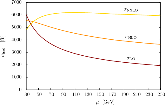
We now show the integrated hadronic cross-sections for the production of the Higgs boson in association with a jet at 8 TeV LHC in the all-gluon channel. We choose to vary the renormalization and factorization scale in the range $\mu_{R}=\mu_{F}=m_{H}/2,~m_{H},~2m_{H}$ . After convolution with the parton luminositites, we obtain⁵⁵ 5 We checked our LO and NLO results against MCFM (gluons only), and found agreement.

\begin{split}&\sigma_{\rm LO}(pp\to Hj)=2713^{+1216}_{-776}~{\rm fb},\\ &\sigma_{\rm NLO}(pp\to Hj)=4377^{+760}_{-738}~{\rm fb},\\ &\sigma_{\rm NNLO}(pp\to Hj)=6177^{-204}_{+242}~{\rm fb}.\end{split}

(138)

We note that NNLO corrections are sizable, as expected from the large NLO $K-$ factor, but the perturbative expansion shows marginal convergence. We also evaluated PDFs error using the full set of NNPDF replicas, and found it to be of order 5% at LO, and of order 1-2% at both NLO and NNLO, similarly to the inclusive Higgs case [78]. The cross-section increases by about sixty percent when we move from LO to NLO and by thirty percent when we move from NLO to NNLO. It is also clear that by accounting for the NNLO QCD corrections we reduce the dependence on the renormalization and factorization scales in a significant way. The scale variation of the result decreases from almost 50% at LO, to 20% at NLO, to less than 5% at NNLO. We also note that a perturbatively-stable result is obtained for the scale choice $\mu\approx m_{H}/2$ . In this case the ratio of the NNLO over the LO cross-section is just $1.5$ , to be compared with $2.3$ for $\mu=m_{H}$ and $3.06$ for $\mu=2m_{H}$ , and the ratio of NNLO to NLO is $1.2$ . It is interesting to point out that a similar trend was observed in the calculation of higher-order QCD corrections to the Higgs boson production cross-section in gluon fusion. It has been pointed out that because of the rapid fall of the gluon PDFs, the production cross section is dominated by the threshold region, thus making $\mu=m_{H}/2$ an excellent choice for the renormalization and factorization scales [81, 14]. The reduced scale dependence is also apparent from Fig. 5, where we plot total cross-section as a function of the renormalization and factorization scale $\mu$ in the region $p_{\perp,j}<\mu<2m_{h}$ .

Finally, we comment on the phenomenological relevance of the “gluons-only” results for cross-sections and $K$ -factors that we reported in this paper. We note that at leading and next-to-leading order, quark-gluon collisions increase the $H+j$ production cross-section by about $30$ percent, for the input parameters that we use in this paper. At the same time, the NLO $K$ -factors for the full $H+j$ cross-section are smaller by about $10-15$ percent than the “gluons-only” $K$ -factors, presumably because quark color charges are smaller than the gluon ones. Therefore, we conclude that the gluon-only results can be used for reliable phenomenological estimates of perturbative $K$ -factors but adding quark channels will be essential for achieving precise results for the $H+j$ cross-section. We plan to return to this issue in the future.

8 Conclusions

In this paper we reported a calculation of the NNLO QCD corrections to the partonic process $gg\to H+{\rm jet}$ . This is one of the first calculations where NNLO QCD corrections are computed to a $2\to 2$ process whose cross-section depends on the implementation of the jet algorithm already at leading order. We believe that $gg\to Hg$ is a sufficiently typical process to expose all non-trivial features of a generic NNLO computation for a $2\to 2$ process at a hadron collider. Indeed, we have used this process to show that the computational technique that we describe in this paper can successfully deal with:

•

a large number of contributing Feynman diagrams;
•

colored particles in the initial and in the final state;
•

collinear subtractions and parton distribution functions;
•

all soft and collinear limits;
•

known helicity matrix elements;
•

spin correlations;
•

a realistic jet algorithm.

The only “non-generic” feature that we benefited from is a much simpler bookkeeping that is required for $gg\to Hg$ compared to the general case computation.

We believe that the techniques reported in this paper that built upon earlier work described in Refs.[55, 56, 63], allow computation of the NNLO QCD corrections to an arbitrary $2\to 2$ process at hadron colliders provided that the corresponding two-loop matrix elements are available. Since this is the case for most of the processes that are desirable to know at NNLO (c.f. the “NNLO wishlist” in Ref. [80]), our results open up a way to perform the required calculations.

On the other hand, it is not entirely clear to us how to extend the computational technology reported in this paper to make it practically applicable to $2\to n$ , $n>2$ processes. In this case, the problem is related to the ${\cal O}(\epsilon)$ parts of the amplitudes and the choice of extra-dimensional components to parametrize four-momenta of unresolved gluons. The point is that in the $2\to 2$ process these details can still be dealt with by brute force, as we did in this paper, but for large $n$ this will be increasingly difficult to do. Therefore, it is an interesting theoretical question to re-formulate this technique in such a way that much of the irrelevant ${\cal O}(\epsilon)$ dependencies is avoided. We hope to return to this point in the future.

Acknowledgments

We thank T. Gehrmann for clarifying to us some results in Ref. [50]. This research is partially supported by the US NSF under grants PHY-0855365 and PHY-1214000, by the U.S. Department of Energy, Division of High Energy Physics, under contract DE-AC02-06CH11357 and the grants DE-FG02-95ER40896 and DE-FG02-08ER4153, and by start-up funds provided by Johns Hopkins University. The research of K.M. is partially supported by Karlsruhe Institute of Technology through a grant provided by its Distinguished Researcher Fellowship program. Calculations reported in this paper were performed on the Homewood High Performance Cluster of Johns Hopkins University or on computing resources provided by Argonne National Laboratory.

Appendix A Appendix

We report here the formulae for the splitting functions and their convolution needed for the renormalization of parton distribution functions at NNLO, as described in Sec. 2.

\begin{split}&P_{gg}^{(0)}(x)=2C_{A}\Bigg[\frac{11}{12}\delta(1-x)+\left[\frac{1}{1-x}\right]_{+}+x(1-x)+\frac{1-x}{x}-1\Bigg]\\ &P_{gg}^{(0)}\otimes P_{gg}^{(0)}=C_{A}^{2}\Bigg[\frac{22}{3}\left[\frac{1}{1-x}\right]_{+}+8\left[\frac{\ln(1-x)}{1-x}\right]_{+}+\left(\frac{121}{36}-\frac{2}{3}\pi^{2}\right)\delta(1-x)\\ &+\frac{4(x^{4}+3x^{2}+1-4x^{3})}{x(x-1)}\ln(x)-\frac{8(2x-1+x^{3}-x^{2})}{x}\ln(1-x)+\frac{2\left(11x^{3}-7x^{2}-4x-11\right)}{3x}\Bigg]\\ &P_{gg}^{(1)}=C_{A}^{2}\Bigg[\left(\frac{8}{3}+3\zeta_{3}\right)\delta(1-x)+\left(\frac{67}{9}-2\zeta_{2}\right)\left[\frac{1}{1-x}\right]_{+}+\frac{4(x^{2}+x+1)^{2}}{x(1+x)}{\rm Li}_{2}(-x)\\ &+\frac{4(3+2x^{2}+4x+2x^{3})}{2(1+x)}\zeta_{2}+\frac{4(x^{2}-x-1)^{2}}{2(1-x^{2})}\ln^{2}(x)-\frac{25}{18}-\frac{109}{18}x\\ &+\left(\frac{4(x^{2}+x+1)^{2}}{x(1+x)}\ln(1+x)-\frac{4(x^{2}-x+1)^{2}}{x(1-x)}\ln(1-x)-\frac{75}{9}+\frac{33}{9}x-\frac{44x^{2}}{3}\right)\ln(x)\Bigg]\end{split}

(139)

References

(1) G. Aad et al. [ATLAS Collaboration], Phys. Lett. B 716, 1 (2012) [arXiv:1207.7214 [hep-ex]].
(2) S. Chatrchyan et al. [CMS Collaboration], Phys. Lett. B 716, 30 (2012) [arXiv:1207.7235 [hep-ex]].
(3) S. Chatrchyan et al. [CMS Collaboration], arXiv:1212.6639 [hep-ex].
(4) LHC Higgs Cross Section Working Group, A. David, A. Denner, M. Duehrssen, M. Grazzini, C. Grojean, G. Passarino and M. Schumacher et al., arXiv:1209.0040 [hep-ph].
(5) S. Dawson, Nucl. Phys. B359, 283 (1991).
(6) A. Djouadi, M. Spira and P. Zerwas, Phys. Lett. B264, 440 (1991).
(7) D. de Florian, M. Grazzini and Z. Kunszt Phys. Rev. Lett. 82, 5209 (1999).
(8) V. Ravindran, J. Smith and V.L. van Neerven, Nucl. Phys. B634, 247 (2002).
(9) C. J. Glosser and C.R. Schmidt, JHEP 0212, 016 (2002).
(10) J.M. Campbell, R.K. Ellis and G. Zanderighi, JHEP 0610, 028 (2006).
(11) J. M. Campbell, R. K. Ellis and C. Williams, Phys. Rev. D 81, 074023 (2010).
(12) H. van Deurzen, N. Greiner et al., arXiv:1301.0493 [hep-ph].
(13) R. V. Harlander and W. B. Kilgore, Phys. Rev. Lett. 88, 201801 (2002) [hep-ph/0201206].
(14) C. Anastasiou and K. Melnikov, Nucl. Phys. B 646, 220 (2002) [hep-ph/0207004].
(15) V. Ravindran, J. Smith and W. L. van Neerven, Nucl. Phys. B 665, 325 (2003) [hep-ph/0302135].
(16) C. Anastasiou, K. Melnikov and F. Petriello, Nucl. Phys. B724, 197 (2005).
(17) S. Catani and M. Grazzini, Phys. Rev. Lett. 98, 222002 (2007); M. Grazzini, JHEP 0802, 043 (2008).
(18) A. Banfi, G.P. Salam and G. Zanderighi, JHEP 1206, 159 (2012).
(19) T. Becher and M. Neubert, JHEP 1207, 108 (2012) [arXiv:1205.3806 [hep-ph]].
(20) F. J. Tackmann, J. R. Walsh and S. Zuberi, arXiv:1206.4312 [hep-ph].
(21) X. Liu and F. Petriello, Phys. Rev. D 87, 014018 (2013) [arXiv:1210.1906 [hep-ph]].
(22) T. Kinoshita, J. Math. Phys. 3, 650 (1962).
(23) T. D. Lee and M. Nauenberg, Phys. Rev. 133, 1549 (1964).
(24) S. Catani and M. H. Seymour, Nucl. Phys. B 485, 291 (1997) [Erratum-ibid. B 510, 503 (1998)] [hep-ph/9605323].
(25) S. Frixione, Z. Kunszt and A. Signer, Nucl. Phys. B 467, 399 (1996) [hep-ph/9512328].
(26) K. Melnikov and F. Petriello, Phys. Rev. D74, 114017 (2006).
(27) K. Melnikov and F. Petriello, Phys. Rev. Lett. 96, 231803 (2006) [hep-ph/0603182].
(28) S. Catani, L. Cieri, G. Ferrera, D. de Florian, M. Grazzini, Phys. Rev. Lett. 103, 082001 (2009).
(29) C. Anastasiou, K. Melnikov and F. Petriello, Phys. Rev. Lett. 93, 262002 (2004).
(30) C. Anastasiou, K. Melnikov and F. Petriello, Phys. Rev. Lett. 93, 032002 (2004).
(31) A. Gehrmann-De-Ridder, T. Gehrmann, E.W.N. Glover and G. Heinrich, JHEP 0712, 094 (2007).
(32) A. Gehrmann-De-Ridder, T. Gehrmann, E.W.N. Glover and G. Heinrich, JHEP 0711, 058 (2007).
(33) S. Weinzierl, Phys. Rev. Lett. 101, 162001 (2008).
(34) C. Anastasiou, K. Melnikov, F. Petriello, JHEP 0709, 014 (2007).
(35) S. Biswas, K. Melnikov, JHEP 1002, 089 (2010).
(36) K. Melnikov, Phys. Lett. B666, 336 (2008).
(37) G. Ferrera, M. Grazzini and F. Tramontano, Phys. Rev. Lett. 107, 152003 (2011) [arXiv:1107.1164 [hep-ph]].
(38) C. Anastasiou, F. Herzog and A. Lazopoulos, JHEP 1203, 035 (2012) [arXiv:1110.2368 [hep-ph]].
(39) S. Catani, L. Cieri, D. de Florian, G. Ferrera and M. Grazzini, Phys. Rev. Lett. 108, 072001 (2012) [arXiv:1110.2375 [hep-ph]].
(40) S. Catani, D. de Florian, and M. Grazzini, Nucl. Phys. B596, 299 (2001).
(41) F. A. Berends and W.T. Giele, Nucl. Phys. B313, 595 (1989).
(42) J.M. Campbell and E.W.N. Glover, Nucl. Phys. B527, 264 (1998).
(43) S. Catani and M. Grazzini, Phys. Lett. B446, 143 (1999).
(44) Z. Bern, et al. Phys. Rev. D60, 116001 (1999).
(45) S. Catani and M. Grazzini, Nucl. Phys. B570, 287 (2000).
(46) S. Catani and M. Grazzini, Nucl. Phys. B591, 435 (2000).
(47) D. A. Kosower, P. Uwer, Nucl. Phys. B563, 477 (1999).
(48) C. Anastasiou, E.W.N. Glover, C. Oleari and M.E. Tejeda-Yeomans, Nucl. Phys. B 601, 318 (2001) [hep-ph/0010212]; 601, 347 (2001) [hep-ph/0011094]; 605, 486 (2001) [hep-ph/0101304];
E.W.N. Glover, C. Oleari and M.E. Tejeda-Yeomans, Nucl. Phys. 605, 467 (2001) [hep-ph/0102201];
C. Anastasiou, E.W.N. Glover and M.E. Tejeda-Yeomans, Nucl. Phys. B 629, 255 (2002) [hep-ph/0201274];
E.W.N. Glover and M.E. Tejeda-Yeomans, JHEP 0306, 033 (2003) [hep-ph/0304169];
E.W.N. Glover, JHEP 0404, 021 (2004) [hep-ph/0401119];
Z. Bern, A. De Freitas and L.J. Dixon, JHEP 0109, 037 (2001) [hep-ph/0109078]; JHEP 0203, 018 (2002) [hep-ph/0201161]; JHEP 0306, 028 (2003) [hep-ph/0304168];
A. De Freitas and Z. Bern, JHEP 0409, 039 (2004) [hep-ph/0409007].
(49) L.W. Garland, T. Gehrmann, E.W.N. Glover, A. Koukoutsakis and E. Remiddi, Nucl. Phys. B 627, 107 (2002) [hep-ph/0112081] and Nucl. Phys. B642, 227 (2002) [hep-ph/0206067].
(50) T. Gehrmann, M. Jaquier, E. W. N. Glover and A. Koukoutsakis, JHEP 1202, 056 (2012) [arXiv:1112.3554 [hep-ph]].
(51) K.G. Chetyrkin, B. Kniehl and M. Steinhauser, Phys. Rev. Lett. 79, 353 (1997); Nucl. Phys. B510, 61 (1998).
(52) S.D. Badger and E.W.N. Glover, P. Mastrolia and C. Williams, JHEP 1001, 036 (2010).
(53) V. Del Duca, A. Frizzo and F. Maltoni, JHEP 0405, 064 (2004); L.J. Dixon, E.W.N. Glover, V.V. Khoze JHEP 0412, 015 (2004).
(54) S. Catani and M. Grazzini, Nucl. Phys. B 570, 287 (2000).
(55) M. Czakon, Phys. Lett. B 693, 259 (2010).
(56) M. Czakon, Nucl. Phys. B849, 250 (2011).
(57) T. Binoth and G. Heinrich, Nucl. Phys. B585, 741 (2000).
(58) T. Binoth and G. Heinrich, Nucl. Phys. B 693, 138 (2004).
(59) C. Anastasiou, K. Melnikov and F. Petriello, Phys. Rev. D69, 076010 (2004).
(60) P. Baernreuther, M. Czakon and A. Mitov, Phys. Rev. Lett. 109, 132001 (2012).
(61) M. Czakon and A. Mitov, JHEP 1212, 054 (2012).
(62) M. Czakon and A. Mitov, JHEP 1301, 080 (2013) [arXiv:1210.6832 [hep-ph]].
(63) R. Boughezal, K. Melnikov and F. Petriello, Phys. Rev. D 85, 034025 (2012) [arXiv:1111.7041 [hep-ph]].
(64) A. Gehrmann-De Ridder, T. Gehrmann and E. W. N. Glover, JHEP 0509, 056 (2005) [hep-ph/0505111]; A. Daleo, T. Gehrmann and D. Maitre, JHEP 0704, 016 (2007) [hep-ph/0612257];J. Currie, E. W. N. Glover and S. Wells, arXiv:1301.4693 [hep-ph]; R. Boughezal, A. Gehrmann-De Ridder and M. Ritzmann, JHEP 1102, 098 (2011) [arXiv:1011.6631 [hep-ph]]; A. Gehrmann-De Ridder, T. Gehrmann and M. Ritzmann, JHEP 1210, 047 (2012) [arXiv:1207.5779 [hep-ph]].
(65) A. G. -D. Ridder, T. Gehrmann, E. W. N. Glover and J. Pires, arXiv:1301.7310 [hep-ph].
(66) J. M. Campbell and R.K. Ellis, Phys. Rev. D 62, 114012 (2000). The MCFM program is publicly available from http://mcfm.fnal.gov.
(67) S. Catani and M. Grazzini, Nucl. Phys. B 591, 435 (2000).
(68) S. Weinzierl, Phys. Rev. D 84, 074007 (2011).
(69) J. Alwall, M. Herquet, F. Maltoni, O. Mattelaer and T. Stelzer, JHEP 1106, 128 (2011) [arXiv:1106.0522 [hep-ph]].
(70) P. Nogueira, J. Comput. Phys. 105, 279 (1993).
(71) J. A. M. Vermaseren, math-ph/0010025.
(72) C. R. Schmidt, Phys. Lett. B413, 391 (1997) [hep-ph/9707448].
(73) R. K. Ellis and G. Zanderighi, JHEP 0802, 002 (2008) [arXiv:0712.1851 [hep-ph]].
(74) G.P. Lepage, Cornell preprint CLNS-80/447.
(75) T. Hahn, Comput.Phys.Commun. 168, 78 (2005).
(76) M. Brucherseifer, F. Caola and K. Melnikov, arXiv:1301.7133 [hep-ph].
(77) M. Brucherseifer, F. Caola and K. Melnikov, arXiv:1302.0444 [hep-ph].
(78) R. D. Ball, V. Bertone, S. Carrazza, C. S. Deans, L. Del Debbio, S. Forte, A. Guffanti and N. P. Hartland et al., Nucl. Phys. B 867, 244 (2013) [arXiv:1207.1303 [hep-ph]].
(79) R. D. Ball et al. [NNPDF Collaboration], Nucl. Phys. B 855, 153 (2012) [arXiv:1107.2652 [hep-ph]].
(80) See a talk by J. Huston at the LoopFest XI, Pittsburgh, May 2012.
(81) M. Kramer, E. Laenen and M. Spira, Nucl. Phys. B 511, 523 (1998) [hep-ph/9611272].

Higgs boson production in association with a jet at next-to-next-to-leading order in perturbative QCD

Abstract

1 Introduction

2 The setup

3 Phase-space parametrizations and sector decomposition

3.1 Phase-space for leading order processes

3.2 Phase-space for next-to-leading order processes

3.3 Phase-space for next-to-next-to-leading order processes

4 Singular limits

4.1 Limits at next-to-leading order

4.2 Limits of double-real emission processes

4.3 Real-virtual corrections

5 Higher-order ϵ\epsilon terms in amplitudes

6 Numerical implementation

7 Checks and final results

8 Conclusions

Appendix A Appendix

References

5 Higher-order $\epsilon$ terms in amplitudes