Blockwise and coordinatewise thresholding to combine tests of different natures in modern ANOVA

Analysis of variance (ANOVA) has something in common with thresholding regression in that ANOVA tests a null hypothesis that some parameters are equal to zero, and thresholding performs model selection by setting some coefficients to zero. This paper exploits this link to derive ANOVA tests based on thresholding.

While ANOVA and tests belong to the general knowledge of a statistician, thresholding is a more recent concept that we now review. A simple way to introduce thresholding and thresholding test is to consider the canonical regression model

where the noise is independent standard Gaussian. A thresholded point estimate of parameters ${\boldsymbol{\theta}}=(\theta_{1},\ldots,\theta_{N})$ is obtained by applying a function $\eta_{\lambda}$ to the data ${\bf Y}=(Y_{1},\ldots,Y_{N})$, that is,

with the property that some or all entries of the estimate are null for a large enough threshold $\lambda$. Defining $(x)_{+}=\max(x,0)$, thresholding can be performed:

• •

  coordinatewise, for instance with soft-thresholding (Donoho and Johnstone, 1994): considering each $n$ in turn, estimate $\theta_{n}$ with

  $$\eta_{\lambda}^{\rm soft}(Y_{n})=\left(1-\frac{\lambda}{|Y_{n}|}\right)_{+}Y_{n}=:\hat{\theta}_{n}.$$

  (3)

• •

  blockwise, for instance with truncated James-Stein thresholding (James and Stein, 1961): considering all entries of ${\bf Y}$ together, estimate ${\boldsymbol{\theta}}$ with

  $$\eta_{\lambda}^{\rm JS+}({\bf Y})=\left(1-\frac{\lambda}{\|{\bf Y}\|_{2}^{2}}\right)_{+}{\bf Y}=:\hat{\boldsymbol{\theta}}.$$

  (4)

The choice of the threshold $\lambda$ plays an important role in the quality of the estimation in regression (see for instance (Donoho and Johnstone, 1994), (Donoho and Johnstone, 1995), (Tibshirani, 1996), (Yuan and Lin, 2006), (Efron, 2004) and (Zou et al., 2007)) or to control the false discovery rate (Benjamini and Hochberg, 1995).

In this article we are interested in linear analysis of variance and testing null hypotheses regarding factors and continuous covariates. We derive new powerful tests based on a thresholded point estimate of the coefficients, and we choose the threshold $\lambda_{\alpha}$ for the test to have the desired level $\alpha$. Since we commented that thresholding can be performed coordinatewise or blockwise, we derive tests based on either coordinate or block thresholding. Or hybrids of both. Two tests are used extensively in ANOVA: Tukey’s multiple comparisons test and Fisher $F$-test. The first one is related to coordinate thresholding and the latter to block thresholding. One goal is to combine Tukey- and Fisher-like tests.

We illustrate the link between thresholding and testing on the canonical model (1) and derive two tests for $H_{0}:\ \theta_{1}=\ldots=\theta_{N}=0$ using a thresholded point estimate. For simplicity we assume for now unit standard deviation for the Gaussian noise. The two tests are:

• •

  based on coordinatewise thresholding (3): clearly, for a sample ${\bf y}$, $\lambda_{\bf y}=\max_{n=1,\ldots,N}|y_{n}|=\|{\bf y}\|_{\infty}$ is the smallest and finite threshold that sets all the estimated parameters to zero. Letting $F_{\Lambda_{0}}$ be the distribution of that statistics under the null hypothesis, and choosing $\lambda_{\alpha}=F_{\Lambda_{0}}^{-1}(1-\alpha)$, the test that rejects $H_{0}$ if $\lambda_{\bf y}>\lambda_{\alpha}$ or, equivalently if at least one entry of the coordinatewise thresholded point estimate $\hat{\boldsymbol{\theta}}({\lambda_{\alpha}})$ is different from zero has the desired level $\alpha$. Here $\lambda_{\alpha}=-\Phi^{-1}([1-\exp\{\log(1-\alpha)/N\}]/2)$ has a closed form expression, otherwise one can estimate it by Monte Carlo. Arias-Castro et al. (2011) call this test a max-test for an obvious reason.

• •

  based on blockwise thresholding (4): likewise, for a sample ${\bf y}$, $\lambda_{\bf y}=\|{\bf y}\|_{2}^{2}$ is the smallest and finite threshold that sets all the estimated parameters to zero. Under the null, that statistics $\Lambda_{0}\sim\chi^{2}_{N}$. Therefore choosing the threshold $\lambda_{\alpha}=F_{\chi^{2}_{N}}^{-1}(1-\alpha)$, the test that rejects $H_{0}$ if $\hat{\boldsymbol{\theta}}({\lambda_{\alpha}})$ is different from the null vector leads to another test of level $\alpha$.

Arias-Castro et al. (2011) studied the asymptotic relative power of both tests under either a dense or a sparse alternative hypothesis $H_{1}$. According to their definition, $H_{1}$ is dense or sparse whether the parameters ${\boldsymbol{\theta}}$ satisfy either $\{\|{\boldsymbol{\theta}}\|_{2}^{2}\geq B\}$ or $\{\|{\boldsymbol{\theta}}\|_{\infty}\geq A\}$ for some positive lower bounds $B$ and $A$, respectively. They proved that the max-test has more power under the sparse alternative.

Another goal of this paper is to derive thresholding-based tests for ANOVA considering either a coordinate or a block thresholding strategy, and see how they relate to and improve on existing tests. Our tests are based on thresholding estimators developed for linear models, and in particular lasso (Tibshirani, 1996), grouped lasso (Yuan and Lin, 2006) and smooth blockwise iterative thresholding (Sardy, 2012). We show how the threshold parameter $\lambda_{\alpha}$ of these estimators can be determined for the thresholding test to have the desired level $\alpha$. Lockhart et al. (2013) consider a sequential approach of testing the significance of the successive lasso coefficients.

Section 2 starts will the simple one-way ANOVA, derives a blockwise and coordinatewise tests, and investigate their relative power under a dense and a sparse alternative. To take the best of both (dense and sparse) alternative worlds, Section 3 derives a single $\alpha$-level test, called O&+ test, that is nearly as powerful as either the blockwise or the coordinatewise tests under both alternatives. Section 4 is concerned with Tukey multiple comparisons test, and proves that it amounts to a coordinate thresholding test. The latter has the advantage of having the exact desired level not only in the balanced situation (like Tukey’s), but also in the unbalanced one (where Tukey’s is conservative), albeit a Monte Carlo estimate of the threshold. Section 5 presents the general framework for iterative thresholding-based tests for ANOVA, for which some coefficients may be thresholded coordinatewise, blockwise or both, depending on the nature of the parameters (fixed effects, interactions, random effects) and on the nature of the alternative hypothesis considered (dense or sparse). Section 6 applies the new test to a real data set modeled by mixed effects. Section 7 proposes another selection of the threshold based on an extension of the universal threshold to satisfy both good estimation and model selection properties. Section 8 draws some conclusions.

To fix notation, consider one-way ANOVA with $T$ treatments and $R$ replications

where $\epsilon_{tr}\stackrel{{\scriptstyle\rm i.i.d.}}{{\sim}}{\rm N}(0,\sigma^{2})$ and the total number of observations is $N=TR$. In matrix notation, (5) is ${\bf Y}=X{\boldsymbol{\mu}}+{\boldsymbol{\epsilon}}$, where $X$ is an $N\times T$ matrix with

The matrix has orthogonal columns since $X^{\rm T}X=R\ I_{T}$. For testing

the most common approach is Fisher’s test based on the pivot

where ${\cal F}_{d_{1},d_{2}}$ is the Fisher distribution with degrees of freedom $d_{1}$ and $d_{2}$, ${\rm RSS}=\|{\bf Y}_{0}-X\hat{\boldsymbol{\mu}}^{\rm LS}\|_{2}^{2}$ with $\hat{\boldsymbol{\mu}}^{\rm LS}=(X^{\rm T}X)^{-1}X^{\rm T}{\bf Y}_{0}$, ${\rm RSS}_{H_{0}}=\|{\bf Y}_{0}-\bar{Y}_{0}{\bf 1}\|_{2}^{2}$ and ${\bf Y}_{0}\sim{\rm N}(\mu{\bf 1},\sigma^{2}I_{N})$. Next section shows that the same test can be derived based on block thresholding.

The relative power of both tests calls for a single test that would be of level $\alpha$ while being as powerful as the best between the block- and coordinate-tests. The following test approaches that goal by defining a point estimate based on joint block- and a coordinate-thresholding on the same parameters.

We now explain the notation $F^{O}$, $F^{+}$ and $F^{O\&+}$. In dimension two, the $\ell_{2}$-ball employed by Fisher block-test is a circle symbolized by ’O’, the two canonical directions employed by coordinate thresholding are the horizontal and vertical directions symbolized by ’+’, and so we call the joint test the O&+ test.

To define the O&+ test, consider the concatenated matrix $[X,X]$ and two sets of coefficients ${\boldsymbol{\theta}}_{1}$ and ${\boldsymbol{\theta}}_{2}$. Block ${\boldsymbol{\theta}}_{1}$ into one block and treat the second coordinatewise. For reason we will explain, rescale the matrix $X$ into $X_{1}=XD_{1}$ and $X_{2}=XD_{2}$, where $D_{1}$ and $D_{2}$ are diagonal. Finally consider the point estimate $\hat{\boldsymbol{\theta}}(\lambda)=(\hat{\boldsymbol{\theta}}_{1}({\lambda}),\hat{\theta}_{2,1}({\lambda}),\ldots,\hat{\theta}_{2,T}({\lambda}))$ defined as a solution to

for a given positive threshold $\lambda$ and smoothness parameter $s\geq 1$, where ${\bf y}_{A}={\bf y}-P_{A}{\bf y}$ as before. The solution to the system is unique if $s>1$ (Sardy, 2012), and has the property that $\hat{\boldsymbol{\theta}}({\lambda})={\bf 0}$ iff $\lambda\geq\max\{\|X_{1}^{\rm T}{\bf y}_{A}\|_{2},\|X_{2}^{\rm T}{\bf y}_{A}\|_{\infty}\}$ for $s\geq 1$. This is a particular case of Lemma 1 proved below, which leads to the following test.

Theorem 3 (O&+ test): Consider model (8) for which we test (7) at a prescribed level $\alpha$. Let ${\bf Y}_{0}\sim{\rm N}(\mu{\bf 1},\sigma^{2}I_{N})$ be the distribution of ${\bf Y}$ under $H_{0}$ and let $\hat{\sigma}$ be a positive estimate of $\sigma$ such that $\hat{\sigma}/\sigma$ is a pivot. Then

is a pivot with distribution $F^{\oplus}_{\Lambda_{0,(2,\infty)}}$. Defining the thresholded point estimate $\hat{\boldsymbol{\theta}}({\bf y}/\hat{\sigma}({\bf y});{\lambda_{\alpha,(2,\infty)}})$ solution to (13) for the observations ${\bf y}$ and setting the threshold $\lambda_{\alpha,(2,\infty)}$ such that $F^{\oplus}_{\Lambda_{0,(2,\infty)}}(\lambda_{\alpha,(2,\infty)})=1-\alpha$, then the test

has level $\alpha$.

Following on Section 2.3 and Table 1 we consider the power of the joint-test under both dense and sparse alternatives as a function of $\theta$ (again assuming $\mu$ and $\sigma$ are known). Figure 1 shows the power function of the block- and coordinate-tests (curve), and estimate them as well for values of $\theta$ on a grid with a Monte-Carlo simulation. We also report the empirical power of the O&+ test on the same grid, which has the remarkable property of performing under both alternatives almost as well as the best of the two individual tests.

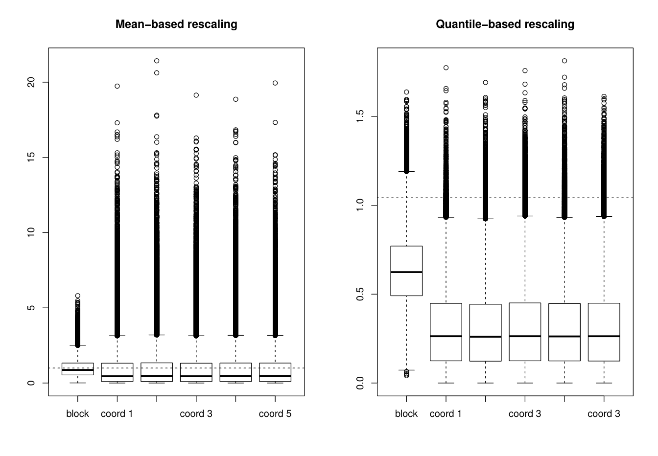
To achieve with a single test a power nearly as good as the best of the two individual tests, rescaling the design matrix $X$ by $D_{1}$ and $D_{2}$ is a crucial step. To allow the joint-test to have the same sensitivity whether the alternative is of the dense or sparse type, we perform the following quantile-based rescaling: we let the matrix corresponding to the block coefficients ${\boldsymbol{\theta}}_{1}$ be $X_{1}=XD_{1}$ where $D_{1}$ is diagonal with entries $1/\lambda_{\alpha,2}$; likewise we let $X_{2}=XD_{2}$ where $D_{2}$ is diagonal with entries $1/\lambda_{\alpha,\infty}$ for the coefficients ${\boldsymbol{\theta}}_{2}$ thresholded coordinatewise. The theoretical values of $\lambda_{\alpha,2}$ and $\lambda_{\alpha,\infty}$ are known (12) in our simple setting, but in more complex settings, we rely on a Monte-Carlo simulation to estimate them. Figure 2 illustrates the advantage of quantile-based rescaling (right), as opposed to mean-based rescaling (left) proposed by Yuan and Lin (2006) for group lasso. The left plot shows that, under the null, the boxplots are centered around their means (horizontal dotted line); because of that rescaling, the distribution of the block statistics $\|X_{1}^{\rm T}{\bf Y}_{0}\|_{2}$ (first boxplot from left) has its largest observations significantly lower than those of the coordinate statistics $|{\bf x}_{2,1}^{\rm T}{\bf Y}_{0}|,\ldots,|{\bf x}_{2,T}^{\rm T}{\bf Y}_{0}|$ (second to sixth boxplots). Consequently, with an alternative hypothesis of the dense type, the joint-test would have low power with that rescaling. Instead, the right plot of Figure 2 shows how quantile rescaling centers the distributions of the block and coordinate statistics around their $(1-\alpha)$-quantile (horizontal dotted line), hence providing the joint test with a homogeneous sensitivity under both dense and sparse alternatives.

When the null hypothesis (6) is rejected, Tukey (1953) is interested in identifying which null hypotheses

caused rejection of (6). His test is dual to intervals

based on the Studentized range distribution ${\cal T}_{T,N-T}$, where $\hat{\sigma}^{2}({\bf y})$ is the unbiased estimate of variance. Here $R_{t}>0$ is the number of replication in treatment $t$ (not necessarily all equal to $R$). The test rejects $H_{0}^{(t,t^{\prime})}$ if zero is not covered by its corresponding interval (16). The level $\alpha$ of the test satisfies that none of the $T(T-1)/2$ tests are rejected with probability $1-\alpha$ under the null hypothesis (6). While the level is exact when $R_{t}=R$ for all $t$, the test is conservative (Hayter, 1984) for unbalanced designs, that is when the number of replication $R_{t}$ differs between treatments.

Tukey’s multiple comparisons test can also be derived based on thresholding and its level can be set to $\alpha$, even when the number of replication $R_{t}$ differs between treatments. To see that, first note that the design matrix is orthogonal with $X^{\rm T}X={\rm diag}(R_{1},\ldots,R_{T})$. Then let $E=(X^{\rm T}X)^{-1}X^{\rm T}$ and $\Delta$ be the $T(T-1)/2\times T$ matrix such that ${\boldsymbol{\delta}}=\Delta{\boldsymbol{\mu}}$ are the pairwise differences. Left multiplying (2) be $\Delta E$ implies $\tilde{\bf y}=X{\boldsymbol{\delta}}+\tilde{\boldsymbol{\varepsilon}}$ with $X=I$, $\tilde{\bf y}=\Delta E{\bf y}$ and $\tilde{\boldsymbol{\varepsilon}}=\Delta E{\boldsymbol{\varepsilon}}$.

The coordinate thresholding estimate defined in (11) can now be applied to that latter model. First rescaling must be performed: the diagonal $D^{2}={\rm diag}(\sigma^{2}\Delta EE^{\rm T}\Delta^{\rm T})$ of the covariance matrix of $\tilde{\boldsymbol{\varepsilon}}$ is not constant, unless $R_{t}=R$ for all $t=1,\ldots,T$. So we standardize $X=I$ such that the marginals of $X^{\rm T}\tilde{\bf y}$ are Gaussian with identical variance under $H_{0}$, by multiplying $X$ by $D^{-1}$. Since the matrix $X=D^{-1}$ is diagonal, the coordinate thresholding estimate defined in (11) has the closed form expression

for all pairs $(t,t^{\prime})$. This thresholded point estimate leads to the following test.

Theorem 4 (Coordinate thresholding test and Tukey multiple comparisons test). Consider model (5) for which we test all null hypotheses (15) at a prescribed level $\alpha$. Let ${\bf Y}_{0}\sim{\rm N}(\mu{\bf 1},\sigma^{2}I_{N})$ be the distribution of ${\bf Y}$ in (5) and let $\hat{\sigma}^{2}$ be the standard unbiased estimate of the variance. Then $\Lambda_{0,\infty}=\|D^{-1}\Delta E{\bf Y}_{0}\|_{\infty}/\hat{\sigma}({\bf Y}_{0})$ is a pivot with distribution $F^{+}_{\Lambda_{0,\infty}}$. Defining the thresholded point estimate $\hat{\boldsymbol{\delta}}({\bf y}/\hat{\sigma}({\bf y});{\lambda_{\alpha,\infty}})$ in (17) for the observations ${\bf y}$ and setting the threshold $\lambda_{\alpha,\infty}$ such that $F^{+}_{\Lambda_{0,\infty}}(\lambda_{\alpha,\infty})=1-\alpha$, then the test

has level $\alpha$. Moreover if $R_{t}=R$ for all treatments, this test is equivalent to Tukey’s range test with the relation ${\cal T}_{T,N-T}(\alpha)=\lambda_{\alpha,\infty}\sqrt{2}$, where $N=RT$.

Proof: the proof that this test has level $\alpha$ is straightforward. For the equivalence to Tukey multiple comparisons test when $R_{t}=R$ for all treatments $t$, note that on the one hand Tukey’s test rejects when at least one interval (16) does not cover zero, or equivalently when $|\bar{y}_{t}-\bar{y}_{t^{\prime}}|-{\cal T}_{T,N-T}(\alpha)\hat{\sigma}({\bf y})/\sqrt{R}\leq 0$ for at least one pair $(t,t^{\prime})$. On the other hand, the thresholding test rejects when $|\tilde{y}_{(t,t^{\prime})}/d_{(t,t^{\prime})}/\hat{\sigma}({\bf y})|\leq\lambda_{\alpha,\infty}$, where $\tilde{y}_{(t,t^{\prime})}=(\Delta E{\bf y})_{(t,t^{\prime})}=\bar{y}_{t}-\bar{y}_{t^{\prime}}$, and all $d_{(t,t^{\prime})}^{2}=2/R$ when $R=R_{t}$. So the thresholding test rejects when $|\bar{y}_{t}-\bar{y}_{t^{\prime}}|\leq\lambda_{\alpha,\infty}\hat{\sigma}({\bf y})\sqrt{2/R}$. So the two tests are equivalent and ${\cal T}_{T,N-T}(\alpha)=\lambda_{\alpha,\infty}\sqrt{2}$. _□

We illustrate the gain in power and oracle property of the thresholding test in comparison to Tukey’s multiple comparisons test on the same Monte Carlo simulation as in Section 3, except that the number of replication in each of the $T=5$ treatments is $(1,5,9,10,10)$ instead of $R_{t}=R=10$ for all treatments. The alternative hypothesis of the form $H_{1}:\ {\boldsymbol{\theta}}=(\theta,0,0,0,0)$ is indexed by the parameter $\theta$ in the range $[0,6]$. In that setting, Tukey’s test is conservative as we observe on the left plot of Figure 3 where the percentage increase of power is plotted as a function of $\theta$. The right plot informs on the number of correct detections, with a target value of $T-1$ non-zero entries guessed correctly. We see on the graph that the thresholding test has slighlty more correct detections on average than Tukey’s conservative test.

If it is not clear to the statistician whether the alternative hypothesis is sparse or dense, then Tukey multiple comparisons test could be turned into an O&+ test as well to have more power under both alternatives.

Finally we considered pairwise contrasts, but the thresholding test could easily be implemented to test other contrasts.

We now consider general ANOVA models which can be written in the form

The matrix $A$ corresponds to the nuisance parameters ${\bf b}$. In the one-way ANOVA considered in the previous section, $A={\bf 1}$ and $b$ is the intercept coefficients, but $A$ can include a large number of parameters we do not want to test. The $N\times P$ matrix $X$ corresponds to the parameters of interest, and is the horizontal concatenation of matrices $X_{1},\ldots,X_{Q}$ corresponding to effects ${\boldsymbol{\theta}}_{1},\ldots,{\boldsymbol{\theta}}_{Q}$, each of respective size $P_{q}$ such that $\sum_{q=1}^{Q}P_{q}=P$. For instance in a one-way ANOVA plus random effects, ${\boldsymbol{\theta}}_{1}$ are the main and ${\boldsymbol{\theta}}_{2}$ random effects, as in the application of Section 6. Another example of concatenated matrices is the joint test of Section 3 with coefficients $({\boldsymbol{\theta}}_{1},\theta_{21},\ldots,\theta_{2T})$ with corresponding matrices $X=[X_{1}{\bf x}_{21}\ldots{\bf x}_{2T}]$. We assume that matrices $A$ and $X_{1},\ldots,X_{Q}$ are all full rank; $X$ needs not be full rank. Moreover we assume the space of the nuisance parameters are not too large, in the sense that all $X_{q}$ must have some components outside the range of $A$.

Our goal is to test the null hypothesis (7), that is test

at a desired level $\alpha$. To derive a threshold-based test, we must define a point estimate that thresholds and is uniquely defined. Sardy (2012) guarantees uniqueness of a thresholding estimator with a linear and invertible reparametrization of (18) into

where each $\tilde{X}_{q}$ must satisfy the orthogonality condition: $\tilde{X}_{q}^{\rm T}\tilde{X}_{q}=d_{q}^{2}I_{P_{q}}$ with $d_{q}>0$. Group lasso is also defined with this condition (Yuan and Lin, 2006), but not necessarily uniquely. Orthogonalization can be achieved with a QR or SVD decomposition, for instance. Testing (19) is equivalent to testing

For a given threshold $\lambda>0$ and a smoothness parameter $s\geq 1$, we introduce the thresholded point estimate $\hat{\boldsymbol{\gamma}}$ defined as a solution (not necessarily unique unless $s>1$) to the following nonlinear system

where ${\bf y}_{A}$ is defined in (9) and ${\cal Q}_{\rm block}$ are the indexes of blocked variables (resp., ${\cal Q}_{\rm coord}$ for variables thresholded coordinatewise), and ${\bf X}_{-(q,t)}$ is the matrix $X$ without column $t$ of block $q$ (Sardy, 2012). This point estimate has the following important property.

Lemma 1: Considering system (22) for given $s\geq 1$ and $\lambda>0$, then

if and only if

In this case, $\hat{\boldsymbol{\gamma}}(\lambda)$ is uniquely defined.

Proof: the implication is straightforward. For the converse, the choice of $\lambda$ in (24) implies ${\bf 0}$ is a solution. The proof is complete if the zero solution is unique. When $s>1$, Sardy (2012) proved uniqueness of the solution to (22). When $s=1$, (22) are the first order optimality conditions to the hybrid lasso-grouped lasso defined as solution to

where $\|{\boldsymbol{\gamma}}\|_{\cal Q}=\sum_{q\in{\cal Q}_{\rm block}}\|{\boldsymbol{\gamma}}_{q}\|_{2}+\sum_{q\in{\cal Q}_{\rm coord}}\|{\boldsymbol{\gamma}}_{q}\|_{1}$ is a hybrid-norm. This cost function $C({\boldsymbol{\gamma}})$ of the above minimization problem is convex in ${\boldsymbol{\gamma}}$, and the solution may not be unique in that case. In fact if two solutions ${\boldsymbol{\gamma}}_{1}$ and ${\boldsymbol{\gamma}}_{2}$ exist then their convex combinations ${\boldsymbol{\gamma}}_{\delta}=\delta{\boldsymbol{\gamma}}_{1}+(1-\delta){\boldsymbol{\gamma}}_{2}$ are also solutions, that is $C({\boldsymbol{\gamma}}_{1})=C({\boldsymbol{\gamma}}_{2})=C({\boldsymbol{\gamma}}_{\delta})=C^{*}$ for all $\delta\in[0,1]$. But suppose $\tilde{X}{\boldsymbol{\gamma}}_{1}\neq\tilde{X}{\boldsymbol{\gamma}}_{2}$, then the strict convexity of $\|\cdot\|_{2}^{2}$ and convexity of the ${\cal Q}$-norm imply that

This contradiction implies that any two solutions must satisfy $\tilde{X}{\boldsymbol{\gamma}}_{1}=\tilde{X}{\boldsymbol{\gamma}}_{2}$, and have the same least squares cost. So their penalty term must be equal: $\lambda\|{\boldsymbol{\gamma}}_{1}\|_{\cal Q}=\lambda\|{\boldsymbol{\gamma}}_{2}\|_{\cal Q}$. Since ${\boldsymbol{\gamma}}_{1}={\boldsymbol{0}}$ is a solution, its ${\cal Q}$-norm is zero. Then necessarily ${\boldsymbol{\gamma}}_{2}={\bf 0}$. _□

The following theorem proposes a test of level $\alpha$ and shows it is a thresholding test since it amounts to testing whether a thresholded point estimate is null or not. Its proof is based on Lemma 1.

Theorem 4 (Thresholding test for ANOVA): Consider model (18) for which we test (19) at a prescribed level $\alpha$. Assume $A$ is full column rank and let $P_{A}$ be the projection in the range of $A$. Let ${\bf Y}_{0}\sim{\rm N}(A{\bf b},\sigma^{2}I_{N})$ be the distribution of ${\bf Y}$ under $H_{0}$ and let $\hat{\sigma}^{2}$ be the standard unbiased estimate of variance. Then

is a pivot with distribution $F_{\Lambda_{0}}$. Letting $\lambda_{\alpha}=F_{\Lambda_{0}}^{-1}(1-\alpha)$, then the test

has level $\alpha$. Moreover defining the thresholded point estimate $\hat{\boldsymbol{\gamma}}({\bf y}/\hat{\sigma}({\bf y});{\lambda_{\alpha}})$ as a solution to (22) for the observation ${\bf y}$, then the test

Rescaling the block matrices $X_{q}$ after orthonormalizing them is a crucial step as we illustrated in Section 3. Quantile rescaling allows the $Q$ blocks to contribute equally to the distribution of the pivot $\Lambda_{0}$ in (25), regardless of their sizes. Quantile rescaling is defined as follows. Given a block $q$ and the orthonormalization $W_{q}$ of $X_{q}$ (with QR or SVD), quantile rescaling applies the same factor to $W_{q}$ and leads to the rescaled matrix:

• •

  $\tilde{X}_{q}=W_{q}d_{q}$, where $1/d_{q}=\lambda_{\alpha,2}^{(q)}$ is the $(1-\alpha)$-quantile of the distribution of $\|W_{q}^{\rm T}{\bf y}_{A}\|_{2}$ under the null, if the corresponding coefficients ${\boldsymbol{\theta}}$ are thresholded blockwise;

• •

  $\tilde{X}_{q}=W_{q}d_{q}$, where $1/d_{q}=\lambda_{\alpha,\infty}^{(q)}$ is the $(1-\alpha)$-quantile of the distribution of $\|W_{q}^{\rm T}{\bf y}_{A}\|_{\infty}$ under the null, if the corresponding coefficients ${\boldsymbol{\theta}}$ are thresholded coordinatewise.

References

- Arias-Castro et al. [2011] E. Arias-Castro, E. J. Candes, and Y. Plan. Global testing under sparse alternatives: Anova, multiple comparisons and the higher criticism. The Annals of Statistics, 39(5):2533–2556, 2011.
- Benjamini and Hochberg [1995] Y. Benjamini and Y. Hochberg. Controlling the false discovery rate: A practical and powerful approach to multiple testing. Journal of the Royal Statistical Society, Series B, Methodological, 57:289–300, 1995.
- Donoho and Jiashun [2004] D. Donoho and J. Jiashun. Higher criticism for detecting sparse heterogeneous mixtures. The Annals of Statistics, 32(3):962–994, 2004.
- Donoho and Johnstone [1994] D. L. Donoho and I. M. Johnstone. Ideal spatial adaptation via wavelet shrinkage. Biometrika, 81:425–455, 1994.
- Donoho and Johnstone [1995] D. L. Donoho and I. M. Johnstone. Adapting to unknown smoothness via wavelet shrinkage. Journal of the American Statistical Association, 90:1200–1224, 1995.
- Donoho et al. [1995] D. L. Donoho, I. M. Johnstone, G. Kerkyacharian, and D. Picard. Wavelet shrinkage: Asymptopia? (with discussion). Journal of the Royal Statistical Society, Series B, 57:301–369, 1995.
- Efron [2004] B. Efron. The estimation of prediction error: Covariance penalties and cross-validation. Journal of the American Statistical Association, 99(467):619–632, 2004.
- Hayter [1984] A. J. Hayter. A proof of the conjecture that the tukey-kramer multiple comparisons procedure is conservative. The Annals of Statistics, 12:61–75, 1984.
- James and Stein [1961] W. James and C. Stein. Estimation with quadratic loss. In Jerzy Neyman, editor, Proceedings of the Fourth Berkeley Symposium on Mathematical Statistics and Probability, Volume 1, pages 361–379. University of California Press, 1961.
- Lockhart et al. [2013] R. Lockhart, J. Taylor, R. J. Tibshirani, and R. Tibshirani. A significance test for the lasso. arXiv:1301.7161, 2013.
- Pinheiro and Bates [2000] J. Pinheiro and D. Bates. Mixed-Effects Models in S and S-PLUS. Springer-Verlag New York, Inc., 2000.
- Sardy [2012] S. Sardy. Smooth blockwise iterative thresholding: a smooth fixed point estimator based on the likelihood’s block gradient. Journal of the American Statistical Association, 107:800–813, 2012.
- Stern [2012] F. Stern. Lasso et estimateurs déerivés: Applications en analyse de la variance. Master’s thesis, Université de Strasbourg, 2012.
- Tibshirani [1996] R. Tibshirani. Regression shrinkage and selection via the lasso. Journal of the Royal Statistical Society, Series B: Methodological, 58:267–288, 1996.
- Tukey [1953] J. W. Tukey. The problem of multiple comparisons. Chapman and Hall, New York, 1953. The Collected Works of John W. Tukey VIII. Multiple comparisons: 1948-1983.
- Yuan and Lin [2006] M. Yuan and Y. Lin. Model selection and estimation in regression with grouped variables. Journal of the Royal Statistical Society, Series B: Statistical Methodology, 68(1):49–67, 2006.
- Zou et al. [2007] H. Zou, T. Hastie, and R. Tibshirani. On the ”degrees of freedom” of the lasso. The Annals of Statistics, 35:2173–2192, 2007.