Solving RG equations with the Lambert $W$ function

The purpose of this paper is to solve generic 2-loop renormalization group (RG) equations exactly using the Lambert $W$ function.[1] The Lambert $W$ function has been introduced previously to solve analytically the 2- and 3-loop RG equations for QCD.[2, 3, 4] (See also [5] for a review of various applications of the Lambert $W$ function to QCD.) We apply the same function to solve generic 2-loop RG equations for theories with a Gaussian fixed point such as the $O(N)$ non-linear sigma model in four dimensions. (This has been partially done in [6].)

In the following we wish to justify our purpose by reminding the reader of the generality of 2-loop RG equations. We consider two examples in four dimensions: QCD and the $\phi^{4}$ theory. Let us consider QCD first.

Let $\Lambda_{0}$ be the ultraviolet cutoff, and $g_{0}^{2}$ be the bare gauge coupling, normalized appropriately. To construct the continuum limit ($\Lambda_{0}\to\infty$) we must give a particular $\Lambda_{0}$ dependence to $g_{0}^{2}$:

where $c=\frac{6\times 153}{33}$ for QCD with no quarks. We can introduce a gauge coupling $g^{2}$, renormalized at a renormalization scale $\mu$, through the $\Lambda_{0}$ independent constant in the denominator. If we choose

then $g^{2}$ satisfies the 2-loop RG equation

exactly.

We next consider the $\phi^{4}$ theory defined by the bare action

with an ultraviolet cutoff $\Lambda_{0}$. This is a theory with the Gaussian fixed point $m_{0}^{2}=\lambda_{0}=0$. We cannot take $\Lambda_{0}$ all the way to infinity, but for $\Lambda_{0}$ large compared with the physical mass, we obtain an almost continuum limit. For a given $\lambda_{0}$, let the critical squared mass be

Then, to get an almost continuum limit, we tune the bare squared mass as

where

Here, the renormalized coupling $\lambda$ is defined so that

The $\lambda_{0}$ dependence of $z_{m}$ and $t_{0}$ is determined so that the theory with given $m^{2}$ and $\lambda$ have no $\lambda_{0}$ dependence except for non-universal contributions suppressed by inverse powers of $\Lambda_{0}$. The parameters $\lambda,m^{2}$ renormalized at the scale $\mu$ satisfy the 2-loop RG equations (1-loop for $m^{2}$) exactly:

We have thus reminded the reader that renormalization schemes exist so that 2-loop RG equations become exact. Hence, solving 2-loop RG equations amounts to solving general RG equations. This paper is organized as follows. In sect. II we solve the generic 2-loop RG equations (9) exactly in terms of the Lambert $W$ function. (This has actually been done already in sect. II.B.1 of [6].) Then, in sec. III, we give the main results of this paper by constructing two physical parameters: one corresponding to the dimensionless coupling and the other corresponding to a physical squared mass. In sect. IV we invert the construction and express the renormalized parameters in terms of the physical parameters. In sect. V, we generalize the exact effective potential in the large $N$ limit of the $O(N)$ linear sigma model [7] to construct a trial effective potential for finite $N$, fully consistent with the 2-loop RG equations.

In this paper we adopt the convention to fix the renormalization scale at $\mu=1$. Hence, a squared mass parameter acquires the canonical dimension $2$ in addition to the anomalous dimension in its RG equation.

We consider the following generic 2-loop RG equation:

and

For example, in the $O(N)$ linear sigma model in four dimensions, we find

for the self-coupling, and

for the squared mass parameter.

In the following we assume $c>0$ and $0\leq x\ll\frac{1}{c}$. Let us define a mass scale by

This satisfies

$\Lambda(x)$ is of the same order as the UV cutoff. We can invert the definition of $\Lambda(x)$ to express $x$ in terms of $\Lambda(x)$. Since

we obtain

where $W$ is the upper branch of the Lambert $W$ function defined by

for $x\geq-\frac{1}{\hbox{e}}$. (See Appendix 1.)

We now define the running parameter $\bar{x}(t;x)$ by

or equivalently by

so that it satisfies both

and the initial condition

(Eq. (20) agrees with (26) of [6] which gives the same result for $c=1$.)

Analogously, the running parameter $\overline{m^{2}}(t;x,m^{2})$ defined by

satisfies

and the initial condition

We now apply the results of the previous section to construct physical parameters. We first observe that the combination

is an RG invariant. We then note that any RG invariant of $x$ and $m^{2}$ can be obtained as a function of the above RG invariant.

Let $x_{\mathrm{ph}}(x,m^{2})$ be the RG invariant satisfying

To obtain an explicit expression for $x_{\mathrm{ph}}(x,m^{2})$, let us write it in the form

where we assume $m^{2}>0$. The condition (27) implies

We can rewrite this as

For small $x\ll 1$, we find $s\gg 1$ for $a+2c>0$, and $-s\gg 1$ for $a+2c<0$. The above equation is solved by the Lambert $W$ function as

We thus obtain the physical coupling $x_{\mathrm{ph}}(x,m^{2})$ as

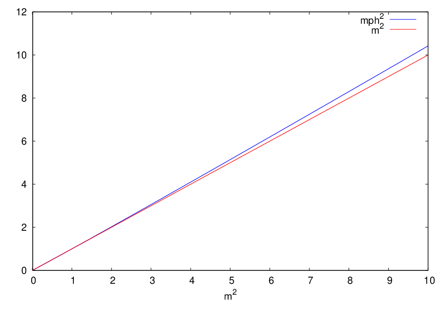
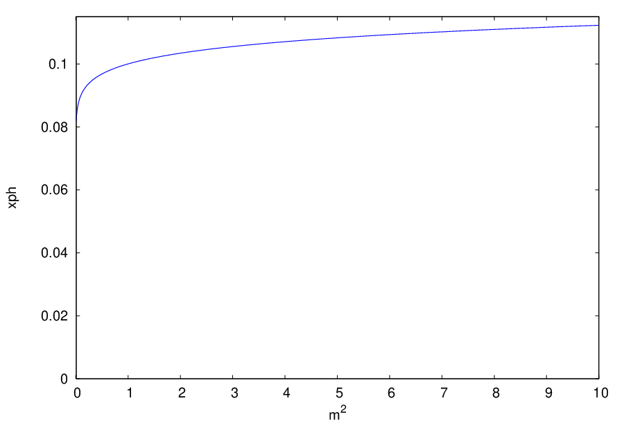
We plot the left-hand side as a function of $m^{2}$ for $x=0.1$ assuming $c=\frac{17}{27}$ and $a=-\frac{1}{3}$.

Though it is not obvious, the physical coupling $x_{\mathrm{ph}}$ admits an asymptotic expansion in powers of $x$. This is because $x_{\mathrm{ph}}$ can be defined by the differential equation

and the initial condition (27). For small $x\ll 1$, we can expand $x_{\mathrm{ph}}$ asymptotically in powers of $x$ in the form

where $p_{n}$ is a polynomial of degree $n$ satisfying $p_{n}(0)=0$. In principle, this can be shown directly from (32), but it is more easily shown from the differential equation (33).

The physical coupling can also be given in the form of a running parameter:

where $t_{\mathrm{ph}}(x,m^{2})$ satisfies

and

To find $t_{\mathrm{ph}}(x,m^{2})$, we use the defining equality $W(x\hbox{e}^{x})=x$ to obtain

Hence, we obtain

In addition to the physical coupling, we can introduce a physical squared mass by

This satisfies

and the initial condition

Using (32), we can rewrite the physical squared mass as

$W$ should be replaced by $W_{-1}$ if $a+2c<0$. The physical squared mass also admits an asymptotic expansion in $x$ just as $x_{\mathrm{ph}}$:

where $q_{n}$ is a polynomial of degree $n$ satisfying $q_{n}(0)=0$.

In the above we have introduced two physical parameters $x_{\mathrm{ph}},m^{2}_{\mathrm{ph}}$ as functions of $x,m^{2}$. We can invert their relations to express $x,m^{2}$ in terms of $x_{\mathrm{ph}},m^{2}_{\mathrm{ph}}$. We first rewrite (32) and (40) as

where we assume $m^{2}>0$, and $W$ should be replaced by $W_{-1}$ if $a+2c<0$. Substituting the second equation into the first to eliminate $m^{2}$, we obtain

This gives

which is valid irrespective of the sign of $a+2c$. Hence, we obtain

Using this result, we then obtain

In [7], the effective potential for the large $N$ limit of the $O(N)$ linear sigma model in four dimensions has been obtained as

where $v$ is the VEV of the scalar field with no anomalous dimension:

In the large $N$ limit, we obtain

so that

In the symmetric phase $m^{2}>0$, $m^{2}_{\mathrm{ph}}(x,m^{2})$ gives the physical squared mass of the scalar fields $\phi^{I}\,(I=1,\cdots,N)$. In the broken phase $m^{2}<0$, the physical squared mass vanishes at

To generalize (51) for a finite $N$, for which $c$ and $a$ are given by (12) and (13), we may try

which is a monotonically increasing function of $v^{2}$. Here $z$ and $g$ are positive functions of the RG invariant

which is well-defined irrespective of the sign of $m^{2}$. Note that the term added to $m^{2}$ satisfies the same RG equation as $m^{2}$:

There is no justification for (56) except that it is fully consistent with RG, and that it gives the correct result in the large $N$ limit where $z$ and $g$ are mere constants:

Note that in the broken phase $m^{2}<0$, the effective potential (or equivalently (56)) is defined only for

Since the right-hand side of (56) is monotonically increasing with $v^{2}$, the effective potential is minimized at $v^{2}=v^{2}_{\mathrm{min}}$.

The main advantage of the assumption (56) is its integrability. To integrate (56) with respect to $v$, we use (43) to write (56) as

where $W$ should be $W_{-1}$ for $a+2c<0$. Denoting

we can rewrite the differential equation for $V_{\mathrm{eff}}$ as

We thus obtain

Using the formulas

where

is the incomplete gamma function, we finally obtain

where

Note that $W$ should be replaced by $W_{-1}$ for $a+2c<0$.

In this paper we have constructed two physical parameters $x_{\mathrm{ph}}$ and $m^{2}_{\mathrm{ph}}$ by solving generic 2-loop RG equations analytically in terms of the Lambert $W$ function. In addition we have constructed explicitly a trial effective action, which is fully consistent with RG, by generalizing the analytic expression for the large $N$ limit of the $O(N)$ linear sigma model in four dimensions.[7] The trial effective potential is, however, at best a wild guess at the true effective potential. Its only merit may be that it gives an intriguing example of what RG improved perturbation theory can produce.

The closed-form analytic expressions for $x_{\mathrm{ph}}$ (given by (32)) and $m^{2}_{\mathrm{ph}}$ (given by (40)) sum the corresponding perturbative series. Further studies may elucidate the precise asymptotic nature of the perturbative expansions, as has been done for QCD.[2, 3]