Next-to-Leading Order Thermal Photon Production in a Weakly Coupled Quark-Gluon Plasma

Jacopo Ghiglieri Affiliation: McGill University, Department of Physics,
3600 rue University, Montreal QC H3A 2T8, Canada Email: jacopo.ghiglieri@physics.mcgill.ca Juhee Hong Affiliation: WCI Center for Fusion Theory, National Fusion Research Institute,
Daejeon 305-806, Korea Email: jhong7@nfri.re.kr Aleksi Kurkela Affiliation: McGill University, Department of Physics,
3600 rue University, Montreal QC H3A 2T8, Canada Email: aleksi.kurkela@mcgill.ca Egang Lu Affiliation: McGill University, Department of Physics,
3600 rue University, Montreal QC H3A 2T8, Canada Email: legang@physics.mcgill.ca Guy D. Moore Affiliation: McGill University, Department of Physics,
3600 rue University, Montreal QC H3A 2T8, Canada Email: guymoore@physics.mcgill.ca and Derek Teaney Affiliation: Department of Physics and Astronomy, Stony Brook University,
Stony Brook, New York 11794-3800, United States Email: derek.teaney@stonybrook.edu

Abstract

We compute the next-to-leading order ${\mathcal{O}}(g)$ correction to the thermal photon production rate in a QCD plasma. The NLO contributions can be expressed in terms of gauge invariant condensates on the light cone, which are amenable to novel sum rules and Euclidean techniques. We expect these technologies to be generalizable to other NLO calculations. For the phenomenologically interesting value of $\alpha_{\mathrm{s}}=0.3$ , the NLO correction represents a 20% increase and has a functional form similar to the LO result.

Keywords

Photons, Hard Probes, Quark-Gluon Plasma, High order calculations, Euclidean methods

1 Introduction

Photon production has long been considered a key “hard probe” for studying the formation and evolution of the quark-gluon plasma in heavy ion collisions. A chief advantage is that the coupling of the plasma to photons is weak, which means that the re-absorption rate of photons is expected to be negligible. Once formed, a photon will escape to the detector, carrying direct information about its formation process unmodified by hadronization or other late time physics.

Experimentally, there are now detailed data on real photon production at RHIC [1, 2, 3] and the LHC [4, 5, 6, 7]. Photons arising from meson decays following hadronization are subtracted from the data experimentally, and the remaining sample of direct photons arises from several (hopefully distinct) processes. There are “prompt” photons produced in the scattering of the partons from the colliding nuclei. The production rate here should be calculable using perturbative QCD [8]. There are also photons associated with the fragmentation of jets and with jet-medium interactions [9, 10], and photons produced by the interaction of excitations of the nearly thermal Quark-Gluon Plasma, which appears to be produced in the collision. The thermal and jet-medium photons are the most interesting (to us) because they represent a signal specifically of the plasma and its evolution.

On the theoretical side, the calculation of the photon production rate from the quark-gluon plasma has mostly been carried out within the context of the perturbative or weak-coupling expansion. The photon emission rate from the plasma was computed to leading order in the logarithm of the strong coupling in 1991, when Kapusta et al and Baier et al computed the rate of Compton and pair annihilation processes [11, 12]. It was later pointed out that this calculation is not complete at leading order, as bremsstrahlung processes arise at the same power of $\alpha_{\rm s}$ [13]. The complete treatment of these processes was completed in 2001, when Arnold, Moore and Yaffe performed a leading-order calculation of the photon production rate from an equilibrium plasma [14, 15]. All these calculations are for the production of photons from a thermal medium, but they are rather easily adapted to include jet-medium interaction photons as well [10].

A leading order calculation begs many questions. By itself it gives no information on its own reliability; we do not know how quickly the perturbative expansion will converge, or what will be the sign of the next correction. There is some concern that a leading order calculation will not be very reliable for the photon production rate. First of all, the coupling is rather large at the modest temperatures achieved in heavy ion collisions. Second, the convergence of other perturbative expansions in the context of finite temperature QCD is not very comforting. For instance, the pressure of the Quark-Gluon Plasma has been computed to very high order in the perturbative expansion [16, 17, 18, 19], with the result that the convergence of the series is rather poor. The pressure is a thermodynamical quantity, as in fact are almost all the quantities computed beyond leading order in the coupling. Among dynamical transport quantities, such as the photon rate and the rather closely related shear viscosity, heavy quark energy loss, and heavy quark diffusion rate, only one quantity is known beyond leading order – the heavy quark diffusion rate [20]. In this case the next-to-leading order corrections prove to be very large. But this case also may not be very representative, since it involves rather different physics than photon production or shear viscosity. Heavy quark diffusion involves particles which are nearly at rest and interact only via spacelike longitudinal gluons. But the other transport coefficients involve species moving at almost the speed of light, exchanging transverse and longitudinal gluons at finite frequencies. They also involve light quarks and their hard thermal loops in a much more direct way than the heavy quark calculation did.

We therefore think it would be extremely useful to compute the photon production rate at next-to-leading order in the coupling. As we have emphasized, this may be of phenomenological interest. And it is most definitely of theoretical interest, since it extends our understanding of the convergence properties of the perturbative expansion for dynamical quantities in the Quark-Gluon Plasma. It also allows us to develop the theoretical tools and understanding which will be needed for other quantities, such as the shear viscosity, in the context of a very cleanly defined calculation. In the remainder of this paper we will present precisely this next-to-leading order calculation of the photon production rate from an equilibrium quark-gluon plasma.

The reason that there are ${\mathcal{O}}(g)$ NLO corrections is because of the complex self-interactions of soft highly occupied gauge fields. As such, all of the NLO corrections arise from the interaction with soft gluons. Since we are concerned with hard photons with $k\geq T$ , the photons must be produced by hard quarks moving at essentially the speed of light. But such quarks only “see” the soft fields in an eikonalized way, feeling soft-sector correlations at lightlike separated points. And bosonic soft correlators at spacelike or lightlike separated points can be determined from correlators of the Euclidean theory; in fact, at leading and next-to-leading order, they are the correlators of the 3-D Euclidean theory, EQCD [21]. Better still, the hard particles are only sensitive, at NLO, to two effects from the soft physics: a shift in the dispersion relation, and transverse momentum exchange. And both of these properties are already known at NLO [22, 21].

The goal of our paper is to derive and explain these facts within the context of the calculation of the NLO photon production rate. We begin with an overview of the calculation in Section 2. We start by reviewing the leading-order calculation, which arises from two distinct kinematic regions, one running from “hard” to “soft” fermionic momenta and one involving “collinear” fermionic momenta. Next we show that the first corrections to the photon production rate arise at ${\mathcal{O}}(g)$ , not at ${\mathcal{O}}(g^{2})$ , and that these corrections arise in several kinematic regions; the collinear region, the “semi-collinear” region which lies between the hard and collinear regions, and the “soft” infrared region. We handle the collinear region in Section 3, the soft region in Section 4, and the “semi-collinear” region in Section 5. We present our results in Section 6.

Because the hard modes experience the soft modes at lightlike separations, we can use analyticity and Euclidean methods very successfully in the calculation. This was impossible in the heavy quark diffusion calculation [20], and means that the photon production calculation is actually simpler than the heavy quark diffusion calculation. This technical development makes it more likely that other transport coefficients, such as shear viscosity, can be computed beyond leading order with a reasonable amount of effort.

On the phenomenological side, we find that there are rather large corrections to the photon production rate from the different kinematic regions, but that they are of both sign and surprisingly similar magnitude. In practice the partial NLO corrections nearly cancel in the full result for the phenomenologically interesting energy range of several times the temperature. As far as we can tell this is an accident. However, the individual (canceling) contributions are also not as large, relative to the leading-order result, as in the heavy quark case. So it appears plausible that NLO corrections are in general not as severe as was feared.

2 Overview of the calculation

The photon production rate is given at leading order in $\alpha$ by

(2\pi)^{3}\frac{d\Gamma_{\gamma}}{d^{3}k}=\frac{1}{2k}\sum_{a}\epsilon^{\mu}_{a}(k)\epsilon^{\nu\,*}_{a}(k)W^{<}_{\mu\nu}(K)\,,

(1)

where $\epsilon^{\mu}_{a}(k)$ are a basis of transverse polarization vectors and $W^{<}_{\mu\nu}(K)$ is the backward Wightman correlator of the electromagnetic current

W^{<}_{\mu\nu}(K)\equiv\int d^{4}Xe^{-iK\cdot X}\left\langle J_{\mu}(0)J_{\nu}(X)\right\rangle.

(2)

Here and throughout the paper capital letters stand for four-vectors, lowercase italic letters for the modulus of the spatial three-vectors and the metric signature is $({-}{+}{+}{+})$ , so that $P^{2}=p^{2}-p^{2}_{0}$ . $K=(k,\mathbf{k})=(k,0,0,k)$ is the lightlike momentum of the photon, which we choose to be oriented along the $z$ axis. We furthermore assume $k{\ \lower-1.2pt\vbox{\hbox{\hbox to0.0pt{$>$\hss}\lower 6.0pt\vbox{\hbox{$\sim$}}}}\ }T$ , which is the validity region of the LO and NLO calculations. We will work perturbatively in the strong coupling $g$ , meaning that we treat the scale $gT$ (the soft scale) as parametrically smaller than the scale $T$ (the hard scale).

Throughout the paper we will often use light-cone coordinates, which we define as $p^{-}\equiv p^{0}-p^{z}$ and $p^{+}\equiv\frac{p^{0}+p^{z}}{2}$ . This normalization is nonstandard, but we find it convenient because $dp^{0}dp^{z}=dp^{+}dp^{-}$ , and because we will frequently encounter cases in which $p^{-}=0$ , in which case $p^{z}=p^{0}=p^{+}$ with our conventions. The transverse coordinates are written as $\mathbf{p}_{\perp}$ , with modulus $p_{\perp}$ .

We finally remark that for convenience we will mostly work in the Keldysh, or $r,a$ , basis of the real-time formalism for the computation of Eq. (2). The two elements of this basis are defined as $\phi_{r}\equiv(\phi_{1}+\phi_{2})/2$ , $\phi_{a}\equiv\phi_{1}-\phi_{2}$ , $\phi$ being a generic field and the subscripts 1 and 2 labeling the time-ordered and anti-time-ordered branches of the Schwinger-Keldysh contour respectively. The propagator is a $2\times 2$ matrix, where one entry is always zero and only one entry depends on the thermal distribution, i.e.,

D=\left(\begin{array}[]{cc}D_{rr}&D_{ra}\\ D_{ar}&D_{aa}\end{array}\right)=\left(\begin{array}[]{ccc}\left(\frac{1}{2}\pm n(p^{0})\right)(D_{R}-D_{A})&&D_{R}\\ D_{A}&&0\end{array}\right),

(3)

where $D_{R}$ and $D_{A}$ are the retarded and advanced propagators, the plus (minus) sign refers to bosons (fermions). $n(p^{0})$ is the corresponding thermal distribution, either $n_{\!\scriptscriptstyle B}(p^{0})=(\exp(p^{0}/T)-1)^{-1}$ for bosons or $n_{\!\scriptscriptstyle F}(p^{0})=(\exp(p^{0}/T)+1)^{-1}$ for fermions. We also define the spectral function as the difference of the retarded and advanced propagators, $\rho\equiv D_{R}-D_{A}$ . We will denote the gluon propagator by $G$ and the quark one $S$ .

We will adopt strict Coulomb gauge throughout. The treatment of soft momenta in propagators and vertices requires the use of Hard Thermal Loop (HTL) resummation [23]. For convenience we list the Coulomb gauge retarded HTL resummed propagators for fermions and gluons in App. A. We will discuss the power-counting rules of the HTL theory with fermions in $r,a$ basis in Section 4.

2.1 Leading-order calculation

At leading order (and also at NLO) in $g$ the photon production rate arises from diagrams where the photon attaches to a single connected quark loop with a number of gluon lines. We denote the momenta flowing in the quark lines that attach to one of the photon vertices $P$ and $K+P$ – see for example Fig. 1. Then the leading order rate arises from three kinematic regimes:

1.

One of the quarks attaching to the photon is on-shell, $(K+P)^{2}\sim g^{2}T^{2}$ , and the other one is far off-shell, $P^{2}\sim T^{2}$ . This is the hard ${2\leftrightarrow 2}$ region.
2.

The photon attaches to one hard on-shell, $(P+K)^{2}\sim g^{2}T^{2}$ , fermionic line and one soft fermionic line with $P^{2}\sim g^{2}T^{2}$ and $P\cdot u\sim gT$ , where $u$ is the rest-frame of the medium. This is the soft ${2\leftrightarrow 2}$ region, and it is the soft limit of the hard ${2\leftrightarrow 2}$ kinematic region.
3.

The photon line attaches to two fermionic lines which are hard ( $P\cdot u\sim T$ and $(K+P)\cdot u\sim T$ ), nearly collinear ( $K\cdot P\sim g^{2}T^{2}$ ), and nearly on-shell ( $P^{2}\sim g^{2}T^{2}$ and $(P+K)^{2}\sim g^{2}T^{2}$ ); this is the collinear region.

The total leading order rate is the sum of these three kinematic regions:

\frac{d\Gamma_{\gamma}}{d^{3}k}\bigg|_{\mathrm{LO}}=\frac{d\Gamma_{\gamma}}{d^{3}k}\bigg|_{\mathrm{hard}}+\frac{d\Gamma_{\gamma}}{d^{3}k}\bigg|_{\mathrm{soft}}+\frac{d\Gamma_{\gamma}}{d^{3}k}\bigg|_{\mathrm{coll}}\,.

(4)

The physics of each of these regions will be summarized in the remainder of this section.

Diagrammatically, the hard ${2\leftrightarrow 2}$ region consists of the simple two-loop diagrams obtained by adding a single gluon to the one-loop diagram for $W^{<}$ , which is kinematically forbidden for a real photon. These diagrams are shown in Fig. 1; their cuts (when all lines are hard) correspond to the ${2\leftrightarrow 2}$ processes $qg\to q\gamma$ (Compton) and $q\overline{q}\to g\gamma$ (annihilation).

Refer to caption — Figure 1: Two-loop diagrams necessary for the evaluation of the ${2\leftrightarrow 2}$ region. The wavy lines are photons, curly lines are gluons and plain lines are quarks. No assumption is made yet on the scaling (hard, soft, collinear…) of the internal lines. The momentum assignments shown here will be used throughout the paper.

In Fig. 2 we show an example diagram and its corresponding cut.¹¹ 1 In our graphical notation the double line represents particles whose momentum is hard, i.e., ${\mathcal{O}}(T)$ or larger, in at least one component. This thus includes not only hard particles, but also collinear and semi-collinear ones. Fig. 3 shows the processes contributing to the sum of the cut diagrams.

The two first (self-energy) diagrams in Fig. 1 receive parametrically equal contributions from all logarithmic momentum scales (up to $T$ ) of the intermediate virtual quark with momentum $P$ . Thus, the naive computation of the diagrams of Fig. 2 leads to a logarithmic infrared divergence. However, this IR divergence is regulated by the physics of screening and collective plasma excitations, and indeed when the momentum $P$ becomes soft, $P\sim gT$ , the self-energy insertion is not anymore a $g$ -suppressed perturbation in the dispersion relation of the intermediate quark and needs to be resummed. This is the soft region. In this kinematic region, the third diagram in Fig. 1 gives a subleading contribution and thus the diagrams that contribute to the leading order result are those shown in Fig. 4. These diagrams can be most conveniently resummed in Hard Thermal Loop -effective theory, and in particular the leading order HTL-resummed diagram is displayed in Fig. 4. The cuts of the diagram correspond to conversion processes, where a soft fermion exchange with the medium converts a hard quark with momentum $K+{\mathcal{O}}(gT)$ into a photon with momentum $K$ . The computation of the resummed diagram will be discussed in detail in Sec. 4, where a sum rule for its evaluation will be introduced.

The soft and the ${\mathrm{hard}}$ regions are smoothly connected and when $gT\ll P\ll T$ , each set of diagrams gives an equivalent and correct description. In a practical calculation one introduces a momentum cutoff for the integrals $gT\ll\mu_{\perp}^{\textrm{LO}}\ll T$ dividing the two regions. Both contributions then individually depend on $\mu_{\perp}^{\textrm{LO}}$ , but this dependence cancels exactly in the sum of the two terms yielding a logarithm of the temperature over the asymptotic mass $m_{\infty}\sim gT$ of the quark.

In [13, 24, 25] it was pointed out that there is another phase space region that contributes at LO besides the ${\mathrm{hard}}$ and soft regions: the collinear region. In this region

•

the momenta of the quark lines are hard, nearly on shell and collinear to each other, i.e., $p^{+}\sim T$ , $p_{\perp}\sim gT$ , and $p^{-}\sim g^{2}T$ such that $P^{2}\sim g^{2}T$ , and
•

the momentum $Q$ of the gluon is spacelike and soft with $q^{+}\sim q_{\perp}\sim gT$ and $q^{-}\sim g^{2}T$ , so that the kinematics of the quarks are unaffected by the gluon.

These constraints force the angles between the quarks and the photon to be small $\sim g$ , and therefore the cuts of the third diagram in Fig. 1 correspond to the bremsstrahlung and pair annihilation processes shown in Fig. 5.

In this case the intermediate virtual quark is almost on shell and thus has a long lifetime of order $\sim 1/g^{2}T$ which is parametrically of the same order as the small angle scattering rate in the plasma $1/\Gamma\sim 1/g^{2}T$ . Hence during the formation of the photon, there is an $\mathcal{O}(1)$ probability that the intermediate quark will undergo one or several additional soft scatterings with the constituents, and processes involving multiple soft scatterings are not suppressed by powers of $g$ . These multiple scatterings lead to destructive interference, that is known as the Landau-Pomeranchuk-Migdal (LPM) effect that leads to an $\mathcal{O}(1)$ suppression of the collinear rate.

In terms of the two-point function these processes correspond to diagrams with the two nearly collinear fermion lines connected with arbitrary number of soft spacelike gluons with same kinematics as $Q$ . In [14, 15] Arnold, Moore and Yaffe (AMY) showed that it is only the ladder-type diagrams shown in Fig. 6 that contribute to a leading order calculation; the factors of $g$ arising from additional vertices are canceled by near on-shell propagators and large statistical factors arising from the gluonic propagators. The near on-shellness of the quark lines makes the diagrams sensitive to the thermal mass $m_{\infty}^{2}\sim g^{2}T^{2}$ and the thermal width $\Gamma\sim g^{2}T$ of the quark lines, which need to be consistently resummed. Furthermore AMY showed how these diagrams can be resummed in terms of a Schrödinger equation type differential equation, and they obtained the complete leading-order results in [15]. In Sec. 3 we will discuss in detail this equation in the context of the treatment of its NLO corrections.

The leading order result arising from the ${\mathrm{hard}}$ , soft and collinear regions can be summarized as [15]

$\displaystyle\frac{d\Gamma_{\gamma}}{d^{3}k}\bigg\|_{{\mathrm{hard}}}$	$\displaystyle=$	$\displaystyle\frac{\mathcal{A}(k)}{(2\pi)^{3}}\left[\ln\left(\frac{T}{\mu_{\perp}^{\textrm{LO}}}\right)+C_{{\mathrm{hard}}}\left(\frac{k}{T}\right)\right]$	(5)
$\displaystyle\frac{d\Gamma_{\gamma}}{d^{3}k}\bigg\|_{{\mathrm{soft}}}$	$\displaystyle=$	$\displaystyle\frac{\mathcal{A}(k)}{(2\pi)^{3}}\left[\ln\left(\frac{\mu_{\perp}^{\textrm{LO}}}{m_{\infty}}\right)\right]$	(6)
$\displaystyle\frac{d\Gamma_{\gamma}}{d^{3}k}\bigg\|_{{\mathrm{coll}}}$	$\displaystyle=$	$\displaystyle\frac{\mathcal{A}(k)}{(2\pi)^{3}}\left[C_{\mathrm{coll}}^{\mathrm{LO}}\left(\frac{k}{T},\kappa\right)\right]$	(7)

\frac{d\Gamma_{\gamma}}{d^{3}k}\bigg|_{\mathrm{LO}}=\frac{\mathcal{A}(k)}{(2\pi)^{3}}\left[\ln\left(\frac{T}{m_{\infty}}\right)+C_{\mathrm{{\mathrm{hard}}}}\left(\frac{k}{T}\right)+C_{\mathrm{coll}}^{\mathrm{LO}}\left(\frac{k}{T},\kappa\right)\right],

(8)

where ${\mathcal{A}}(k)$ is the leading-log coefficient of the photon production rate

{\mathcal{A}}(k)=2\alpha_{\rm EM}\frac{m_{\infty}^{2}}{k}n_{\!\scriptscriptstyle F}(k)\sum_{s}d_{\scriptscriptstyle R}q_{s}^{2}\quad\left(=\frac{4\alpha_{\rm EM}n_{\!\scriptscriptstyle F}(k)g^{2}T^{2}}{3k}\,\mbox{for QCD with $uds$ quarks}\right).

(9)

Here $d_{\scriptscriptstyle R}$ is the dimension of the quark’s representation ( $d_{\scriptscriptstyle R}=N_{c}$ in the fundamental representation of $SU(N_{c})$ ), $q_{s}$ is its abelian charge, and the sum runs over the number of light fermions flavors, $N_{f}$ . The parameter $\kappa$ is the square of the ratio of $m_{\infty}^{2}=g^{2}T^{2}C_{\scriptscriptstyle R}/4$ to the Debye mass $m_{\scriptscriptstyle D}^{2}=g^{2}T^{2}(C_{\scriptscriptstyle A}+N_{f}T_{R})/3$ at leading order in $g$ . $\kappa$ encodes the dependence on the number of colors and light flavors in the plasma, i.e.

\kappa\equiv\frac{m_{\infty}^{2}}{m_{\scriptscriptstyle D}^{2}}=\frac{3C_{\scriptscriptstyle R}}{4(C_{\scriptscriptstyle A}+T_{R}N_{f})}\quad\left(=\frac{2}{6+N_{f}}\mbox{ for QCD}\right),

(10)

where $C_{\scriptscriptstyle R}$ and $C_{\scriptscriptstyle A}$ are the quadratic Casimirs of the representations of the quarks and gluons respectively, and $T_{R}$ is the index of the representation of the quarks.²² 2 $C_{\scriptscriptstyle R}=(N_{c}^{2}-1)/2N_{c}$ and $T_{R}=1/2$ for quarks in the fundamental representation, and $T_{A}=C_{\scriptscriptstyle A}=N_{c}$ for the adjoint representation of $SU(N_{c})$ . The definition of $m_{\infty}^{2}$ is discussed in Appendix B.4.

The functions $C_{\mathrm{{\mathrm{hard}}}}(k/T)$ and $C_{\mathrm{coll}}^{\mathrm{LO}}(k/T,\kappa)$ describe the momentum dependence of the ${\mathrm{hard}}$ and collinear regions and have to be obtained numerically, the former by integrating the matrix elements for the hard processes folded over the thermal distributions and the latter by solving the integral equation for collinear processes. For further convenience we list the parametrization of these functions as given in [15] for a $N_{c}=3$ QCD plasma with $N_{f}$ flavors:

	$\displaystyle C_{\mathrm{{\mathrm{hard}}}}\left(\frac{k}{T}\right)$	$\displaystyle\approx$	$\displaystyle\frac{1}{2}\ln\left(\frac{2k}{T}\right)+0.041\frac{T}{k}-0.3615+1.01e^{-1.35k/T},\quad 0.2<\frac{k}{T},$		(11)
	$\displaystyle C_{\mathrm{coll}}^{\mathrm{LO}}\left(\frac{k}{T},\kappa\right)$	$\displaystyle\approx$	$\displaystyle\frac{1}{\sqrt{\kappa}}\left[\frac{0.316\ln(12.18+T/k)}{\left(k/T\right)^{3/2}}+\frac{0.0768k/T}{\sqrt{1+k/(16.27T)}}\right],\quad 0.2<\frac{k}{T}<50.$

We conclude this overview of the leading-order calculation by noting that the momentum integration regions that contribute here are best identified by their scaling in terms of $P$ . In Fig. 7 we map these momentum regions in the $(p^{+},p_{\perp})$ plane. The scaling of $p^{-}$ can be obtained from momentum conservation.

2.2 Next-to-leading order corrections

At next to leading order, the full result is a sum of the leading order rate and its ${\mathcal{O}}(g)$ correction

\displaystyle\frac{d\Gamma_{\gamma}}{d^{3}k}\bigg|_{{\mathrm{LO}}+{\mathrm{NLO}}}

\displaystyle=

\displaystyle\frac{d\Gamma_{\gamma}}{d^{3}k}\bigg|_{{\mathrm{LO}}}+\frac{d\delta\Gamma_{\gamma}}{d^{3}k}.

(13)

As in the leading order calculation, the NLO rate arises from distinct kinematic regions and the NLO correction can be parametrized as

\displaystyle\frac{d\delta\Gamma_{\gamma}}{d^{3}k}

\displaystyle=

\displaystyle\frac{d\delta\Gamma_{\gamma}}{d^{3}k}\bigg|_{{\mathrm{soft}}}+\frac{d\delta\Gamma_{\gamma}}{d^{3}k}\bigg|_{{\mathrm{coll}}}+\frac{d\delta\Gamma_{\gamma}}{d^{3}k}\bigg|_{{\mathrm{semi-coll}}}.

(14)

The soft and collinear regions are the same kinematic regions as in the leading-order calculation, while the semi-collinear region is an additional kinematic region whose contribution starts at NLO.

In the hard region, corrections come about by adding an extra loop to the diagrams shown in Fig. 1. As long as momenta stay hard, we need not worry about these corrections, which are suppressed by a factor of $g^{2}$ relative to the leading-order result.

However, both the soft propagator and the location of the quasiparticle pole at hard momenta have ${\mathcal{O}}(g)$ corrections, and thus diagrams that are sensitive to these quantities may also receive ${\mathcal{O}}(g)$ corrections. Indeed, in the collinear case the individual rungs in the ladder resummation are soft gluons, and the collinear quarks are near the quasiparticle pole. Consequently, the parameters of the collinear integral equation that record the soft gluon scattering rate and the quasiparticle masses, ${\mathcal{C}}(q_{\perp})$ and $m_{\infty}^{2}$ , are modified at NLO. The structure of the NLO correction arising from the collinear region is then

\frac{d\delta\Gamma_{\gamma}}{d^{3}k}\bigg|_{{\mathrm{coll}}}=\frac{d\delta\Gamma_{\gamma}}{d^{3}k}\bigg|_{\delta m}+\frac{d\delta\Gamma_{\gamma}}{d^{3}k}\bigg|_{\delta C},

(15)

where the first term is due to a ${\mathcal{O}}(g)$ shift in $m_{\infty}^{2}$ , and the second term arises from a one-loop ${\mathcal{O}}(g)$ correction to the soft scattering kernel, ${\mathcal{C}}(q_{\perp})$ . In Section 3 we will discuss these corrections in detail, as well as two $\mathcal{O}\left(g\right)$ subregions where the collinear phase space starts to overlap with the soft and semi-collinear regions, requiring subtractions.

In the soft region, the addition of an extra soft gluon to the diagram in Fig. 4 results in the diagrams shown in Fig. 8, which represent an $\mathcal{O}\left(g\right)$ correction to the conversion process.

In particular, wherever a gluon ends on a soft fermion line, all momenta flowing in that quark-gluon vertex are of order $gT$ . This causes the bare and HTL vertices to be of the same order, requiring the inclusion of the HTL vertex, as shown in the first and last diagrams in Fig. 8. Furthermore, the two-quark, two-gluon HTL gives rise to a new topology, the second diagram in that figure.

The complicated analytic structure of the HTL vertices and propagators, with their branch cuts and imaginary parts, as well as the non-trivial functional dependence on the momenta, would in principle make the calculation of the diagrams in Fig. 8 technically intricate and only amenable to a multi-dimensional numerical integration. However, in Sec. 4 we develop a set of sum rules using the analytic properties of these amplitudes, which are in turn related to causality. These sum rules, as we shall show, simplify the calculation dramatically leading to an analytical result.

When evaluating these soft diagrams we must correct the LO treatments of the soft region to avoid double counting. Note that the first diagram in Fig. 8 is the soft limit of the HTL self-energy already included in the soft-LO calculation, see Fig. 4. The HTL self-energy used at LO includes an integral over the hard thermal loop momentum $Q$ which extends down to zero, with ${\mathcal{O}}(g)$ of the contribution arising from the soft region of integration where the HTL approximation is no longer valid. Thus, while the first diagram in Fig. 8 has already been included at LO, the LO treatment is incorrect at NLO. To avoid double counting and to correct this mistreatment we have to subtract this soft-loop part of the HTL calculation. We do this by subtracting a counterterm diagram shown in Figure 9.

Similarly, in the calculation of the leading order collinear rate, an ${\mathcal{O}}(g)$ part of the $p^{+}$ integration arises from the kinematic region where $p^{+}$ is soft and overlaps with the soft region. For example, the LO treatment of the collinear bremsstrahlung diagram shown Fig. 5 integrates over the momentum fraction of the final state quark, and is incorrect when this momentum fraction is ${\mathcal{O}}(g)$ . This region is correctly dealt with by the soft graphs of Fig. 8, and the mistreated LO collinear contribution must be subsequently subtracted. The structure of the soft region at NLO is then

\displaystyle\frac{d\delta\Gamma_{\gamma}}{d^{3}k}\bigg|_{{\mathrm{soft}}}

\displaystyle=

\displaystyle\frac{d\delta\Gamma_{\gamma}}{d^{3}k}\bigg|_{{\mathrm{soft}}}^{\rm{diags.}}-\frac{d\Gamma_{\gamma}}{d^{3}k}\bigg|_{\textrm{soft}}^{\textrm{subtr.}},

(16)

where the first term arises from the difference of the diagrams in Fig. 8 and Fig. 9 and the second is the soft part of the leading order collinear rate. The complete treatment of the soft region, including the diagrams of Fig. 8 and all necessary subtractions, is given in Section 4.

Finally, a third region contributes to the NLO rate, corresponding to the uncharted, wedge-shaped area in Fig. 7 between the ${\mathrm{hard}}$ and collinear regions where $Q\sim gT$ is soft and the scaling of $P$ obeys $p^{+}\sim T$ , $p^{-}\sim gT$ and $p_{\perp}\sim\sqrt{g}T$ , so that $P^{2}\sim gT^{2}\sim P\cdot K$ — this is the semi-collinear region. This region is closer to the mass shell and closer to collinearity with $K$ than the hard region (where $P^{2}\sim T^{2}\sim P\cdot K$ ), but farther from the mass shell and less collinear than the collinear region (where $P^{2}\sim g^{2}T^{2}\sim P\cdot K$ ).³³ 3 Naive power-counting arguments suggest that this region, with the exchange of a soft $Q\sim gT$ gluon, should actually be leading order. But there is a cancellation between the diagrams shown in Fig. 1. This cancellation, pointed out in footnote 5 of Ref. [14], renders this phase space region ${\mathcal{O}}(g)$ with respect to the leading contributions. The physical processes in this region are characterized by the sign of $Q^{2}$ . For timelike gluon momenta the semi-collinear contribution can be seen as a correction to the ${\mathrm{hard}}$ region from the emission/absorption of soft gluons on their massive, quasiparticle plasmon poles. In the spacelike region, on the other hand, one can interpret this contribution as a less collinear emission, the angle being now $\sqrt{g}$ instead of $g$ . This in turn implies a formation time of the order of $1/(gT)$ , much shorter than the inverse scattering rate. The LPM effect is then not relevant in this region.

The leading order treatment of the collinear region also mistreats the semi-collinear region by an ${\mathcal{O}}(g)$ amount, and the part of the leading order collinear rate arising from the semi-collinear region again needs to be subtracted. Also, the leading order hard calculation receives an ${\mathcal{O}}(g)$ mistreated contribution from the semi-collinear regions so that the structure of the semi-collinear correction becomes

\displaystyle\frac{d\delta\Gamma_{\gamma}}{d^{3}k}\bigg|_{{\mathrm{semi-coll}}}

\displaystyle=

\displaystyle\frac{d\delta\Gamma_{\gamma}}{d^{3}k}\bigg|_{{\mathrm{semi-coll}}}^{\rm{diags.}}-\frac{d\Gamma_{\gamma}}{d^{3}k}\bigg|_{{\mathrm{semi-coll}}}^{\textrm{coll. subtr.}}-\frac{d\Gamma_{\gamma}}{d^{3}k}\bigg|_{{\mathrm{semi-coll}}}^{\textrm{hard subtr.}}.

(17)

The complete treatment of the semi-collinear region is given in Section 5.

We conclude this section by mapping the NLO integration regions in the $(p^{+},p_{\perp})$ plane in Fig. 10, in analogy the LO map in Fig. 7.

3 The collinear region

The evaluation of the collinear region at leading order requires the resummation of an infinite number of soft gluon exchanges through an integral equation. Such an equation was derived by Arnold, Moore, and Yaffe [14, 15] and gives rise to a LO contribution to the photon production rate of

$\displaystyle\frac{d\Gamma_{\gamma}}{d^{3}k}\bigg\|_{{\mathrm{coll}}}$	$\displaystyle=$	$\displaystyle\frac{{\mathcal{A}}(k)}{(2\pi)^{3}}\int_{-\infty}^{\infty}dp^{+}\left[\frac{(p^{+})^{2}+(p^{+}{+}k)^{2}}{(p^{+})^{2}(p^{+}{+}k)^{2}}\right]\>\frac{n_{\!\scriptscriptstyle F}(k{+}p^{+})[1-n_{\!\scriptscriptstyle F}(p^{+})]}{n_{\!\scriptscriptstyle F}(k)}$	(18)
		$\displaystyle\times\frac{1}{g^{2}C_{\scriptscriptstyle R}T^{2}}\int\frac{d^{2}p_{\perp}}{(2\pi)^{2}}\>{\rm Re}\>2\mathbf{p}_{\perp}\cdot{\bf{f}}(\mathbf{p}_{\perp},p^{+},k)\,,$	(18)
$\displaystyle 2\mathbf{p}_{\perp}$	$\displaystyle=$	$\displaystyle i\delta E\;{\bf{f}}(\mathbf{p}_{\perp})+\int\frac{d^{2}q_{\perp}}{(2\pi)^{2}}\>{\mathcal{C}}(q_{\perp})\Big[{\bf{f}}(\mathbf{p}_{\perp})-{\bf{f}}(\mathbf{p}_{\perp}{+}{\bf{q}}_{\perp})\Big]\,,$	(19)
$\displaystyle\delta E$	$\displaystyle=$	$\displaystyle\frac{k(p_{\perp}^{2}+m_{\infty}^{2})}{2p^{+}(k{+}p^{+})}\,.$	(20)

Here $\delta E=E_{\mathbf{p}+\mathbf{k}}-E_{\mathbf{p}}-k$ is the eikonalized energy difference between having a quark of energy corresponding to a momentum of $k+p$ and having a quark of energy corresponding to momentum $p$ with a photon of energy $k$ . ${\mathcal{C}}(q_{\perp})$ is the differential soft scattering rate, which at leading order reads [14, 26]

{\mathcal{C}}(q_{\perp})=g^{2}C_{\scriptscriptstyle R}\int\frac{dq^{0}dq_{z}}{(2\pi)^{2}}2\pi\delta(q^{0}-q_{z})G^{rr}_{\mu\nu}(Q)v_{k}^{\mu}v_{k}^{\nu}=g^{2}C_{\scriptscriptstyle R}T\frac{m_{\scriptscriptstyle D}^{2}}{q_{\perp}^{2}(q_{\perp}^{2}{+}m_{\scriptscriptstyle D}^{2})}\,,

(21)

where $v_{k}^{\mu}\equiv(1,0,0,1)$ and $G_{\mu\nu}^{rr}$ is the cut HTL gluon propagator.

The physical interpretation of this expression is as follows. Photon production involves a current operator insertion in the amplitude, followed by time evolution, and then a current insertion in the conjugate amplitude. At times between the current insertions, the density matrix contains an off-diagonal term with a quark with momentum $p^{+},\mathbf{p}_{\perp}$ and a photon of momentum $k$ in the amplitude, but a quark of momentum $(p^{+}{+}k),\mathbf{p}_{\perp}$ in the conjugate amplitude. The size for this entry in the density matrix is ${\bf{f}}(\mathbf{p}_{\perp})$ and Eq. (19) is the time-integrated evolution equation for this amplitude; $\delta E$ represents the phase accumulation because the state in the amplitude and conjugate amplitude do not have the same energy, while the ${\mathcal{C}}(q_{\perp})$ term describes the effect of scattering processes on the evolution of the density matrix. The second line in Eq. (18) describes the overlap of the current operator on this density matrix element. The term in square brackets in the first line of Eq. (18) is the DGLAP splitting kernel.

The NLO corrections to this leading order calculation arise from an ${\mathcal{O}}(g)$ correction to thermal mass and to the differential soft scattering rate. These contributions, like the LO contribution, need to be solved for numerically. The most convenient way to do so is to Fourier-transform Eq. (19) to impact parameter space, where the integral equation turns into a differential equation with mixed boundary conditions. This will be discussed in subsection 3.2. First we find the behavior of Eq. (18), Eq. (19) at small $p^{+}$ and at large $p_{\perp}$ , which we need as counterterms in Eqs. (16) and (17). We can find these analytically by perturbing Eq. (19) in $\delta E$ .

3.1 Leading order subtractions: $\Gamma_{\gamma}\,\vline\,_{{\mathrm{semi-coll}}}^{{\rm coll.}\,\,{\rm subtr.}}$ and $\Gamma_{\gamma}\,\vline\,_{{\mathrm{soft}}}^{\rm{subtr.}}$

In the leading order calculation of the collinear rate in Eq. (18), the integral over $p^{+}$ extends artificially all the way down to $p^{+}\lesssim gT$ ; and the $p_{\perp}$ integral extends up to $p_{\perp}\gg gT$ , contrary to the definition of the collinear kinematic region. In these regions, the integrals start to probe the soft and semi-collinear regions, respectively. There, the assumptions made in arriving at Eq. (18) and Eq. (19) start to break down, so that a more detailed analysis is needed. To find the leading order contribution we simply extend the $p^{+}$ integral to zero and the $p_{\perp}$ integral to infinity; then when we handle the $p^{+}\sim gT$ and $p_{\perp}^{2}\sim gT^{2}$ regions more carefully, we will subtract the (incorrect) amount already included in this way in the leading-order calculation, via the subtractions of Eqs. (16) and (17). So let us evaluate Eq. (18), Eq. (19) in these regions.

In the soft and semi-collinear regions, one finds that $\delta E\sim gT$ , and therefore in these regions the first $\delta E$ term in Eq. (19) is larger than the second ${\mathcal{C}}(q_{\perp})$ term. Hence, the evaluation of Eq. (18) and Eq. (19) can be simplified by working to first order in ${\mathcal{C}}(q_{\perp})$ . Physically this is because, if the opening angle becomes large ${\mathcal{O}}(\sqrt{g})$ or if an external quark becomes soft and therefore scatters at a large angle, then the formation time becomes $\sim 1/gT$ , parametrically shorter than the mean time between scatterings $\sim 1/g^{2}T$ . Therefore the LPM effect becomes subleading and the rate is determined by the single scattering rate.

In order to solve Eq. (18) by perturbing in $\delta E^{-1}$ write ${\bf{f}}={\bf{f}}_{1}+{\bf{f}}_{2}+\ldots$ with ${\bf{f}}_{1}\propto(\delta E)^{-1}$ , ${\bf{f}}_{2}\propto(\delta E)^{-2}$ etc. and evaluate iteratively:

2\mathbf{p}_{\perp}=i\delta E\,{\bf{f}}_{1}(\mathbf{p}_{\perp})\quad\Rightarrow\quad{\bf{f}}_{1}=\frac{2\mathbf{p}_{\perp}}{i\delta E(\mathbf{p}_{\perp})},

(22)

which gives zero in Eq. (18) because it is imaginary. Substituting ${\bf{f}}_{1}$ into the collision term to determine ${\bf{f}}_{2}$ , we get

	$\displaystyle 0$	$\displaystyle=$	$\displaystyle i\delta E(\mathbf{p}_{\perp}){\bf{f}}_{2}(\mathbf{p}_{\perp})+\int\frac{d^{2}q_{\perp}}{(2\pi)^{2}}{\mathcal{C}}(q_{\perp})\left[{\bf{f}}_{1}(\mathbf{p}_{\perp})-{\bf{f}}_{1}(\mathbf{p}_{\perp}+{\bf{q}}_{\perp})\right]\,,$
	$\displaystyle{\bf{f}}_{2}(\mathbf{p}_{\perp})$	$\displaystyle=$	$\displaystyle\frac{2}{\delta E(\mathbf{p}_{\perp})}\int\frac{d^{2}q_{\perp}}{(2\pi)^{2}}{\mathcal{C}}(q_{\perp})\left(\frac{\mathbf{p}_{\perp}}{\delta E(\mathbf{p}_{\perp})}-\frac{\mathbf{p}_{\perp}+{\bf{q}}_{\perp}}{\delta E(\mathbf{p}_{\perp}+\mathbf{q}_{\perp})}\right).$		(23)

Since this term is real, it contributes to Eq. (18). The next term ${\bf{f}}_{3}$ is again imaginary, and ${\bf{f}}_{4}$ is ${\mathcal{O}}(g)$ in the regions of interest and therefore negligible. Integrating over $p_{\perp}$ as in Eq. (18) and symmetrizing the resulting expression with respect to $p_{\perp},(p_{\perp}{+}q_{\perp})$ , we find⁴⁴ 4 This symmetrization is natural, indeed necessary, from the point of view of the momentum labeling which we introduced on the diagrams shown in Fig. 1. Namely, the $1/(\delta E(\mathbf{p}_{\perp}))^{2}$ term corresponds to the first diagram there (self-energy on the lower line), the $1/(\delta E(\mathbf{p}_{\perp}{+}\mathbf{q}_{\perp}))^{2}$ term is the next diagram (self-energy on the top line), and the cross-terms are the cat eye diagram. In terms of Fig. 5, for the bremsstrahlung diagram the $1/(\delta E(\mathbf{p}_{\perp}))^{2}$ term is the diagram shown, the $1/(\delta E(\mathbf{p}_{\perp}{+}\mathbf{q}_{\perp}))^{2}$ term is the square of the diagram where the gluon attaches after the photon, and the cross-term is the interference term between these diagrams. Not performing the symmetrization corresponds to evaluating one of the diagrams with different momentum assignments on the external lines.

\int\frac{d^{2}p_{\perp}}{(2\pi)^{2}}2\,\mathbf{p}_{\perp}\cdot{\bf{f}}_{2}(\mathbf{p}_{\perp})=2\int\frac{d^{2}q_{\perp}d^{2}p_{\perp}}{(2\pi)^{4}}{\mathcal{C}}(q_{\perp})\left(\frac{\mathbf{p}_{\perp}}{\delta E(\mathbf{p}_{\perp})}-\frac{\mathbf{p}_{\perp}+{\bf{q}}_{\perp}}{\delta E(\mathbf{p}_{\perp}+\mathbf{q}_{\perp})}\right)^{2}.

(24)

We now turn to the application of this equation to the specifics of the soft and semi-collinear limits.

3.1.1 The soft fermion, collinear contribution

We now consider Eq. (18) in the region where either $p^{+}$ or $p^{+}+k^{+}$ is small. We will show that the integrand goes over to a constant, so ${\mathcal{O}}(g)$ of the contribution to $\Gamma_{\gamma}$ arises from the region where $p^{+}$ is ${\mathcal{O}}(g)$ . This $p^{+}$ -independent behavior will turn into a linearly divergent subtractive counterterm when we evaluate the soft region.

First consider Eq. (18) in the regime where $p^{+}$ is formally ${\mathcal{O}}(T)$ but soft, $p^{+}\ll T$ and $p^{+}\ll k$ . In this case we can approximate Eq. (18) as

\frac{d\Gamma_{\gamma}}{d^{3}k}\bigg|_{\textrm{soft}}^{\textrm{subtr.}}=\frac{{\mathcal{A}}(k)}{(2\pi)^{3}}\int dp^{+}\frac{1}{(p^{+})^{2}}\frac{1}{2}\;\frac{1}{g^{2}C_{\scriptscriptstyle R}T^{2}}\int\frac{d^{2}p_{\perp}}{(2\pi)^{2}}{\rm Re}\>2\mathbf{p}_{\perp}\cdot{\bf{f}}(\mathbf{p}_{\perp},p^{+})\,.

(25)

Upon plugging the soft- $p^{+}$ limit of $\delta E$ , i.e.,

\delta E=\frac{p_{\perp}^{2}+m_{\infty}^{2}}{2p^{+}}\,,

(26)

into Eq. (24) we obtain

\int\frac{d^{2}p_{\perp}}{(2\pi)^{2}}2\,\mathbf{p}_{\perp}\cdot{\bf{f}}_{2}(\mathbf{p}_{\perp})=8(p^{+})^{2}\int\frac{d^{2}q_{\perp}d^{2}p_{\perp}}{(2\pi)^{4}}{\mathcal{C}}(q_{\perp})\left(\frac{\mathbf{p}_{\perp}}{p_{\perp}^{2}{+}m_{\infty}^{2}}-\frac{\mathbf{p}_{\perp}{+}{\bf{q}}_{\perp}}{(\mathbf{p}_{\perp}{+}{\bf{q}}_{\perp})^{2}+m_{\infty}^{2}}\right)^{2}.

(27)

In terms of $p^{+}$ scaling, we see that Eq. (19) gives $(p^{+})^{2}$ times a $p^{+}$ -independent function. This cancels the $(p^{+})^{-2}$ in the integrand in Eq. (25), so indeed the integrand in Eq. (25) is independent of $p^{+}$ at small $p^{+}$ . Since $p^{+}\sim gT$ represents ${\mathcal{O}}(g)$ of the phase space of $p^{+}$ values available, this region therefore represents an ${\mathcal{O}}(g)$ fraction of the photon production rate, as claimed.

The region where $p^{+}{+}k$ is soft gives an identical contribution. Inserting $2{\bf{f}}_{2}$ into Eq. (25) we then get

	$\displaystyle\frac{d\Gamma_{\gamma}}{d^{3}k}\bigg\|_{\textrm{soft}}^{\textrm{subtr.}}$	$\displaystyle=$	$\displaystyle\frac{{\mathcal{A}}(k)}{(2\pi)^{3}}\int_{-\mu^{+}}^{+\mu^{+}}dp^{+}\>\frac{8}{T}\!\int\frac{d^{2}p_{\perp}d^{2}q_{\perp}}{(2\pi)^{4}}\frac{m_{\scriptscriptstyle D}^{2}}{q_{\perp}^{2}(q_{\perp}^{2}+m_{\scriptscriptstyle D}^{2})}$		(28)
			$\displaystyle\hskip 91.04872pt\times\left(\frac{\mathbf{p}_{\perp}}{p_{\perp}^{2}+m_{\infty}^{2}}-\frac{\mathbf{p}_{\perp}+{\bf{q}}_{\perp}}{(\mathbf{p}_{\perp}{+}{\bf{q}}_{\perp})^{2}+m_{\infty}^{2}}\right)^{2},$		(28)

where we introduced a regulator $gT\ll\mu^{+}\ll T$ for the linear divergence.

3.1.2 The semi-collinear fermion, collinear contribution

The semi-collinear region represents another ${\mathcal{O}}(g)$ contribution to the integral in Eq. (18). As in the previous case, the approximations that lead to that equation are no longer valid when $P$ becomes semi-collinear ( $p_{\perp}\to\sqrt{g}T$ , $p^{-}\sim gT$ ). This limit is then incorrectly described by Eq. (18) and, as in the previous subsection, we need to derive its limit in order to subtract it from the semi-collinear region, where this momentum scaling will be correctly treated.

We can again use Eq. (24), but now there is an additional simplification; $p_{\perp}^{2}\gg m_{\infty}^{2}$ and $|p_{\perp}|\gg|q_{\perp}|$ . Therefore we can drop $m_{\infty}^{2}$ and work to lowest order in $q_{\perp}$ , which is

	$\displaystyle\int\frac{d^{2}p_{\perp}}{(2\pi)^{2}}2\,\mathbf{p}_{\perp}\cdot{\bf{f}}_{2}(\mathbf{p}_{\perp})$	$\displaystyle=$	$\displaystyle 2\int\frac{d^{2}p_{\perp}d^{2}q_{\perp}}{(2\pi)^{4}}{\mathcal{C}}(q_{\perp})\frac{q_{\perp}^{2}}{(\delta E(p_{\perp}))^{2}}$		(29)
		$\displaystyle=$	$\displaystyle 2\int\frac{d^{2}p_{\perp}}{(2\pi)^{2}}\;\frac{4(p^{+})^{2}(p^{+}+k)^{2}}{k^{2}p_{\perp}^{4}}\int\frac{d^{2}q_{\perp}}{(2\pi)^{2}}\,q_{\perp}^{2}\,{\mathcal{C}}(q_{\perp}).$		(29)

When plugged in Eq. (18), this yields

	$\displaystyle\frac{d\delta\Gamma_{\gamma}}{d^{3}k}\bigg\|_{{\mathrm{semi-coll}}}^{\textrm{coll subtr.}}$	$\displaystyle=$	$\displaystyle 2\frac{{\mathcal{A}}(k)}{(2\pi)^{3}}\int dp^{+}\left[\frac{(p^{+})^{2}+(p^{+}+k)^{2}}{(p^{+})^{2}(p^{+}+k)^{2}}\right]\frac{n_{\!\scriptscriptstyle F}(k+p^{+})[1-n_{\!\scriptscriptstyle F}(p^{+})]}{n_{\!\scriptscriptstyle F}(k)}$		(30)
			$\displaystyle\times\frac{1}{g^{2}C_{\scriptscriptstyle R}T^{2}}\int\frac{d^{2}p_{\perp}}{(2\pi)^{2}}\,\frac{4(p^{+})^{2}(p^{+}+k)^{2}}{k^{2}p_{\perp}^{4}}\int\frac{d^{2}q_{\perp}}{(2\pi)^{2}}\,q_{\perp}^{2}\,{\mathcal{C}}(q_{\perp})\,.$		(30)

The $p_{\perp}$ integration is power $p_{\perp}$ divergent and the $q_{\perp}$ integral is log UV divergent. This is not surprising, since this expression was obtained based on $q_{\perp}\ll p_{\perp}$ .

3.2 NLO corrections to the collinear regime: $\delta\Gamma_{\gamma}\,\vline\,_{\delta m}$ and $\delta\Gamma_{\gamma}\,\vline\,_{\delta C}$

Even at leading order Eq. (19) has to be solved numerically in order to get the collinear contribution. The most convenient way to do so is by Fourier transforming $\mathbf{p}_{\perp}$ and ${\bf{q}}_{\perp}$ into impact-parameter variables, as first proposed in [27]. The advantages are, first, that the convolution over the collision kernel ${\mathcal{C}}(q_{\perp})$ becomes a product, turning an integral equation into a differential equation; second, that the source on the left-hand side becomes a boundary condition at ${\bf{b}}=0$ ; and third, that the desired final integral, Eq. (18), becomes a boundary value of the ODE solution. Specifically, defining

{\bf{f}}({\bf{b}})=\int\frac{d^{2}q_{\perp}}{(2\pi)^{2}}e^{i{\bf{b}}\cdot{\bf{q}}_{\perp}}{\bf{f}}(\mathbf{q}_{\perp})\,,

(31)

we have

{\rm Re}\>\int\frac{d^{2}p_{\perp}}{(2\pi)^{2}}2\mathbf{p}_{\perp}\cdot{\bf{f}}(\mathbf{p}_{\perp})={\rm Im}(2\nabla_{b}\cdot{\bf{f}}(b))\,,

(32)

and Eq. (19) becomes

-2i\nabla\delta^{2}({\bf{b}})=\frac{ik}{2p^{+}(k+p^{+})}\Big(m_{\infty}^{2}-\nabla_{b}^{2}\Big){\bf{f}}({\bf{b}})+{\mathcal{C}}^{\prime}(b){\bf{f}}({\bf{b}})\,,

(33)

with⁵⁵ 5 Note that ${\mathcal{C}}^{\prime}(b)$ is not the Fourier transform of ${\mathcal{C}}(q_{\perp})$ , but rather the difference between the Fourier transform at zero ${\bf{b}}$ and at finite ${\bf{b}}$ , which is better behaved (in particular, not sensitive to the divergent total cross-section). Alternately, we can redefine ${\mathcal{C}}(q_{\perp})$ to have a negative delta function at $q_{\perp}=0$ , normalized so that its integral $\int d^{2}q_{\perp}{\mathcal{C}}(q_{\perp})$ vanishes, in which case Eq. (19) does not need the first term in square brackets, and ${\mathcal{C}}^{\prime}(b)$ is minus the Fourier transform of ${\mathcal{C}}(q_{\perp})$ .

{\mathcal{C}}^{\prime}(b)\equiv\int\frac{d^{2}q_{\perp}}{(2\pi)^{2}}\Big(1-e^{i{\bf{b}}\cdot{\bf{q}}_{\perp}}\Big){\mathcal{C}}(q_{\perp})\,.

(34)

In the collinear regime the ${\mathcal{O}}(g)$ corrections enter then in two places: both the effective thermal mass squared $m_{\infty}^{2}$ and the collision kernel ${\mathcal{C}}(q_{\perp})$ get ${\mathcal{O}}(g)$ corrections which modify Eq. (33),

	$\displaystyle m^{2}_{\infty,\rm LO+NLO}$	$\displaystyle=$	$\displaystyle m_{\infty}^{2}+\delta m_{\infty}^{2},$		(35)
	$\displaystyle{\mathcal{C}}^{\prime}_{\rm LO+NLO}(b)$	$\displaystyle=$	$\displaystyle{\mathcal{C}}^{\prime}(b)+\delta{\mathcal{C}}^{\prime}(b).$		(36)

The computation of the NLO thermal mass from [22] is rederived in Appendix B.4. The NLO collision kernel is computed in [21] in momentum space; in Appendix C we perform the Fourier transformation into impact parameter space.

Eq. (33) is then solved perturbatively, by treating ${\bf{f}}({\bf{b}})$ formally as an expansion in powers of $\delta m_{\infty}^{2},\delta{\mathcal{C}}$ ; ${\bf{f}}({\bf{b}})={\bf{f}}_{0}({\bf{b}})+{\bf{f}}_{1}({\bf{b}})+\ldots$ , and expanding to first order. The zero-order expression is just Eq. (33), while at the linear order the expression reads

0=\left(\frac{ik}{2p^{+}(k+p^{+})}\Big(m_{\infty}^{2}-\nabla_{b}^{2}\Big)+{\mathcal{C}}^{\prime}(b)\right){\bf{f}}_{1}({\bf{b}})+\left(\frac{ik\,\delta m_{\infty}^{2}}{2p^{+}(k+p^{+})}+\delta{\mathcal{C}}^{\prime}(b)\right){\bf{f}}_{0}({\bf{b}})\,,

(37)

where the leading order solution ${\bf{f}}_{0}({\bf{b}})$ acts as a source term in the differential equation for ${\bf{f}}_{1}({\bf{b}})$ .

When evaluating Eq. (33) one must deal with mixed boundary conditions; the function ${\bf{f}}({\bf{b}})$ must decay to zero as ${\bf{b}}\rightarrow\infty$ (one boundary condition), and it must yield the correct normalization

\nabla_{b}^{2}{\bf{f}}_{0}({\bf{b}})=\frac{4p^{+}(k{+}p^{+})}{k}\nabla\delta^{2}({\bf{b}})

(38)

at zero. This is done by evolving the differential equation starting at large ${\bf{b}}$ , with starting data which ensure that the solution will decay away as ${\bf{b}}\rightarrow\infty$ but with an arbitrary normalization. One then solves the differential equation going in towards the origin, generally resulting in a mis-scaled solution. But this solution can be multiplied by a complex constant so that Eq. (38) is satisfied. Similarly, when solving Eq. (37) for ${\bf{f}}_{1}({\bf{b}})$ , the boundary condition that ${\bf{f}}_{1}({\bf{b}})$ should decay at large ${\bf{b}}$ is not enough to fix the solution completely; so one generically gets a solution which is a mixture of the solution to Eq. (37) with correct boundary condition $\lim_{{\bf{b}}\rightarrow 0}\nabla^{2}{\bf{f}}_{1}({\bf{b}})=0$ , plus a multiple of the homogeneous solution (that is, the solution of Eq. (37) at ${\bf{f}}_{0}=0$ ) with the wrong boundary condition at zero. But the homogeneous solution is proportional to ${\bf{f}}_{0}$ , which is known; so it can be subtracted to obtain the solution with correct boundary condition.

We solved Eq. (37) as a function of $k/T$ . The results can be parametrized as follows:

$\displaystyle\frac{d\delta\Gamma_{\gamma}}{d^{3}k}\bigg\|_{{\mathrm{coll}}}$	$\displaystyle=$	$\displaystyle\frac{d\delta\Gamma_{\gamma}}{d^{3}k}\bigg\|_{\delta m}+\frac{d\delta\Gamma_{\gamma}}{d^{3}k}\bigg\|_{\delta C},$	(39)
$\displaystyle\frac{d\delta\Gamma_{\gamma}}{d^{3}k}\bigg\|_{\delta m}$	$\displaystyle=$	$\displaystyle\frac{{\mathcal{A}}(k)}{(2\pi)^{3}}\Big[\frac{\delta m_{\infty}^{2}}{m_{\infty}^{2}}C_{\mathrm{coll}}^{\delta m}\left(\frac{k}{T},\kappa\right)\Big]\,,$	(40)
$\displaystyle\frac{d\delta\Gamma_{\gamma}}{d^{3}k}\bigg\|_{\delta C}$	$\displaystyle=$	$\displaystyle\frac{{\mathcal{A}}(k)}{(2\pi)^{3}}\Big[\frac{g^{2}C_{\scriptscriptstyle A}T}{m_{\scriptscriptstyle D}}C_{\mathrm{coll}}^{\delta{\mathcal{C}}}\left(\frac{k}{T},\kappa\right)\Big]\,.$	(41)

where

\frac{\delta m_{\infty}^{2}}{m_{\infty}^{2}}=-\frac{2m_{\scriptscriptstyle D}}{\pi T}.

(42)

The fitting functions read

$\displaystyle C^{\delta m}_{\rm coll}(x)$	$\displaystyle=$	$\displaystyle\left(\frac{2/9}{\kappa}\right)^{0.25}\Big(-0.3664/x-0.08478-0.0799\,\log(x)$	(43)
		$\displaystyle+0.0315\,x-0.0050\,x\log(x)-0.0681\,(\log(x))^{2}\Big),$	(43)
$\displaystyle C^{\delta C}_{\rm coll}(x)$	$\displaystyle=$	$\displaystyle(-0.7207-0.8236\delta\kappa+3.986\delta\kappa^{2})/x$	(44)
		$\displaystyle+(0.7056+0.0998\delta\kappa-1.186\delta\kappa^{2})$
		$\displaystyle+(-0.8309-0.2610\delta\kappa+2.247\delta\kappa^{2})\log(x)$
		$\displaystyle+(0.12305-0.0108\delta\kappa-0.2871\delta\kappa^{2})\,x$
		$\displaystyle+(-0.01777+0.00148\delta\kappa+0.0434\delta\kappa^{2})x\log(x)$
		$\displaystyle+(0.2804-0.0369\delta\kappa-0.2375\delta\kappa^{2})\log(x)^{2}$
		$\displaystyle+(-0.0702+0.00440\delta\kappa+0.1149\delta\kappa^{2})\log(x)^{3}\,,$

with $\delta\kappa\equiv\kappa-2/9$ . The fitting functions have a relative error smaller than 2% for $N_{f}=3$ QCD ( $\kappa=2/9$ ) in the momentum range $0.5<x<70$ . In the range $0.15<\kappa<0.35$ the relative error is less than 5%.

We will present most of the numerical results, for different values of the parameters such as the coupling, in the exposition of the final results in Sec. 6. Here we just show in Fig. 11 the size of the mass correction, $[\delta m_{\infty}^{2}/m_{\infty}^{2}]C_{\mathrm{coll}}^{\delta m}(k/T,\kappa)$ , and the collision kernel correction, $[g^{2}C_{\scriptscriptstyle A}T/m_{\scriptscriptstyle D}]C_{\mathrm{coll}}^{\delta{\mathcal{C}}}(k/T,\kappa)$ , relative to the the LO collinear result, $C_{\mathrm{coll}}^{\mathrm{LO}}(k/T)$ . The NLO correction $\delta C_{\mathrm{coll}}(k/T)$ is an ${\mathcal{O}}(100\%)$ correction for most of the considered range.

4 The soft region

To introduce the NLO calculation, we begin by reproducing the soft-momentum part of the leading-order calculation introducing the notation. We perform the leading order calculation using novel sum rule technology, which admits a generalization to the NLO calculation.

4.1 Leading-order evaluation and introduction to the fermionic sum rules

The most straightforward approach to the leading-order calculation is to evaluate the trace of the Wightman correlator $W^{<}(K)\equiv g^{\mu\nu}W^{<}_{\mu\nu}(K)$ in Eq. (1) directly in the $1,2$ basis. However, it turns out that the NLO calculation is much simpler to perform in the $r,a$ basis, so we will instead use the $r,a$ basis also at leading order. The object that is most conveniently calculated in the $r,a$ basis is the retarded (advanced) correlator, which is related to the backward Wightman function via the KMS relation

W^{<}(K)=2n_{\!\scriptscriptstyle B}(k)\>{\rm Im}\>iW_{R}(K)=n_{\!\scriptscriptstyle B}(k)(W_{R}(K)-W_{A}(K))\,.

(45)

At leading order, $W_{R}(K)$ and $W_{A}(K)$ each arise from two $r,a$ assignments of the one loop diagram, shown in Figure 12. Our graphical notation for the $r,a$ assignments follows the one in [28]: we draw outgoing arrows for $a$ fields at vertices and incoming ones for $r$ fields. For the $rr$ propagator, rather than drawing two arrows pointing in opposite directions, we omit to draw them; this should cause no confusion. The double lines refer to hard $(K+P)\sim T$ propagators whereas the single lines refer to soft $P\sim gT$ HTL propagators. The different $r,a$ assignments of resummed HTL propagators are easily obtained from the retarded ones listed in App. A by using Eq. (3).

The cut ( $rr$ ) soft line carries a factor of $-n_{\!\scriptscriptstyle F}(p^{0})+1/2\ll 1$ and is therefore suppressed;⁶⁶ 6 It is also odd in $p^{0}$ and will be even more suppressed when averaging over $p^{+}\rightarrow-p^{+}$ . we may therefore drop the two diagrams containing cut soft lines. Summing the other diagrams gives the difference between retarded and advanced propagators on the soft line. This difference is the spectral function $\rho\equiv S_{R}-S_{A}$ . Also the cut line can be expressed in terms of the spectral function; $S_{rr}(K+P)=(\frac{1}{2}-n_{\!\scriptscriptstyle F}(k^{0}+p^{0}))\rho(K+P)$ . We approximate this statistical function as $\frac{1}{2}-n_{\!\scriptscriptstyle F}(k^{0}+p^{0})\simeq\frac{1}{2}-n_{\!\scriptscriptstyle F}(k)$ and use the identity

n_{\!\scriptscriptstyle B}(k)\left(1-2n_{\!\scriptscriptstyle F}(k)\right)=n_{\!\scriptscriptstyle F}(k)\,.

(46)

Bringing everything together,

W^{<}(K)=\sum_{s}\frac{q^{2}_{s}e^{2}d_{\scriptscriptstyle R}n_{\!\scriptscriptstyle F}(k)}{2}\int\frac{d^{4}P}{(2\pi)^{4}}\textrm{Tr}\left[\gamma_{\mu}\rho(K+P)\gamma^{\mu}\rho(P)\right].

(47)

If we had evaluated $W^{<}$ directly without going to the $r,a$ basis we would have written this down immediately.

Now we evaluate Eq. (47) expanding in $P\sim gT\ll K\sim T$ . This expansion will enforce eikonality on the hard line, which is essential for the sum rules described below. It is convenient to write each propagator in terms of its components of positive and negative chirality-to-helicity ratio:

\rho(P)=h^{+}_{P}\rho^{+}(P)+h^{-}_{P}\rho^{-}(P)\,,\qquad h_{P}^{\pm}\equiv\frac{\gamma^{0}\mp\hat{p}\cdot\vec{\gamma}}{2}\,,

(48)

with $\hat{p}={\bf{p}}/p$ . For the hard line, we use an eikonal approximation

\rho^{+}(P{+}K)\simeq 2\pi\delta(v_{k}\cdot P)=2\pi\delta(p^{-})\,,\qquad\rho^{-}(P{+}K)=2\pi\delta(p^{0}+k+|{\bf{p}}{+}{\bf{k}}|)\simeq 0\,,

(49)

and thus the hard line is a function of $p^{-}$ only. Using this delta function simplifies the traces, which we expand in small $P$ :

\textrm{Tr}\left[\gamma_{\mu}h^{+}_{\mathbf{k}+\mathbf{p}}\gamma^{\mu}h^{\pm}_{\mathbf{p}}\right]=2\left(1\mp\frac{p^{+}}{p}\right)\mp 2\frac{p_{\perp}^{2}}{pk}\pm p^{+}\frac{3p_{\perp}^{2}}{pk^{2}}+\mathcal{O}\left(\frac{p^{3}}{k^{3}}\right).

(50)

We insert the leading-order piece of this trace into Eq. (47), finding

W^{<}(K)=2\sum_{s}q^{2}_{s}e^{2}d_{\scriptscriptstyle R}n_{\!\scriptscriptstyle F}(k)\int\frac{dp^{+}d^{2}p_{\perp}}{(2\pi)^{3}}\left[\left(1{-}\frac{p^{+}}{p}\right)\rho^{+}(p^{+}\!,p_{\perp})+\left(1{+}\frac{p^{+}}{p}\right)\rho^{-}(p^{+}\!,p_{\perp})\right]\!.

(51)

The factor of two in front takes care of the kinematic region where $K+P$ is soft and $P$ is hard, which gives the same result after a shift of integration variables.

Next consider the $p^{+}$ integration in Eq. (51). We will perform the integral using analyticity methods similar to those discussed in App. B. The key is that Eq. (51) involves $\rho(p^{-},p^{+},p_{\perp})=S_{R}(p^{-},p^{+},p_{\perp})-S_{A}(p^{-},p^{+},p_{\perp})$ . Due to causality, the retarded and advanced functions are analytic in any timelike or null momentum variable in the upper and lower half planes respectively, generalizing the familiar analyticity properties of these functions in $p^{0}$ [21]. In particular, $S_{R}(p^{-},p^{+},p_{\perp})$ is analytic in the upper half of the complex $p^{+}$ plane, while holding $p^{-}$ and $p_{\perp}$ fixed. We are therefore free to deform the $p^{+}$ integration contour: instead of integrating just above and below the real axis for $S_{R}$ and $S_{A}$ respectively, we integrate along an arc at large $p^{+}$ where $gT\ll p^{+}\ll T$ – see Figure 13. Along these arcs the integrand has a remarkably simple behavior, which can be obtained by expanding the HTL propagator listed in App. A, yielding

\left(1-\frac{p^{+}}{p}\right)S^{+}(p^{+},p)+\left(1+\frac{p^{+}}{p}\right)S^{-}(p^{+},p)\bigg|_{|p^{+}|\to+\infty}=\frac{i}{p^{+}}\frac{m_{\infty}^{2}}{p_{\perp}^{2}+m_{\infty}^{2}}+\mathcal{O}\left(\frac{1}{(p^{+})^{2}}\right).

(52)

Integrating along the arcs at positive and negative $\mathrm{Im}(p^{+})$ for the retarded and advanced contributions one then obtains

W^{<}(K)=2\sum_{s}q^{2}_{s}e^{2}d_{\scriptscriptstyle R}n_{\!\scriptscriptstyle F}(k)\int\frac{d^{2}p_{\perp}}{(2\pi)^{2}}\frac{m_{\infty}^{2}}{p_{\perp}^{2}+m_{\infty}^{2}}\,.

(53)

A numerical integration of Eq. (51) agrees perfectly with this expression. This result was also recently obtained in [29].

To summarize, the reason why it is possible to deform the $p^{+}$ integration can be understood diagrammatically from Fig. 12. When evaluating $W_{R}$ and $W_{A}$ (the first and third diagrams in Fig. 12), the soft fermionic lines are either fully retarded or fully advanced, since soft $rr$ fermionic propagators are suppressed. This is seen from the flow of arrows on soft fermionic lines, which indicates the $r,a$ assignments. Thus, since the cut hard line is eikonal and is only a function of $p^{-}$ and not $p^{+}$ , the $p^{+}$ integration is over either a fully retarded or fully advanced function and can be deformed away from the real axis.

It is worth noting that, while each of the two components $(1\mp p^{+}/p)S^{\pm}(p^{+},p)$ presents poles separately at $p^{+}=\pm ip_{\perp}$ and branch cuts in $(-i\infty,-ip_{\perp})$ , $(ip_{\perp},i\infty)$ , their sum is analytic for $\mathrm{Im}(p^{+})\neq 0$ . This must be so as our sum rule is based on causality; but the chirality-to-helicity decomposition is not Lorentz covariant, so the individual terms need not respect causality. This can be seen from the properties

S^{+}(-P)=S^{-\,*}(P)\,,\qquad S^{-}(-P)=S^{+\,*}(P)\,,

(54)

from which one can also see that the sum of the two components is covariant and does respect causality.

To constrain the integral to the soft region only, the $p^{+}$ integral should be cut off at a finite momentum scale $\mu^{+}\gg gT$ . However, if we cut off the integral at a finite $\mu^{+}\gg gT$ , the ${\mathcal{O}}((p^{+})^{-n})$ subleading corrections to Eq. (52) give rise to $(gT/\mu^{+})^{n-1}$ suppressed corrections. But these will be canceled by corrections which will arise when we perform the calculation of the region above $\mu^{+}$ , since the total result should be $\mu^{+}$ independent. Therefore we need not compute them.

The $d^{2}p_{\perp}$ integration in Eq. (53) should be cut off at some large momentum $gT\ll\mu^{\mathrm{LO}}_{\perp}\ll T$ , where it should match with the contribution from the hard region. The explicit expression reads

\frac{d\Gamma_{\gamma}}{d^{3}k}\bigg|_{\mathrm{soft}}=\frac{\mathcal{A}(k)}{2(2\pi)^{3}}\ln\left(\frac{(\mu^{\mathrm{LO}}_{\perp})^{2}}{m_{\infty}^{2}}+1\right)\approx\frac{\mathcal{A}(k)}{(2\pi)^{3}}\ln\frac{\mu^{\mathrm{LO}}_{\perp}}{m_{\infty}},

(55)

which agrees with the original calculations of the LO soft region in [11, 12].⁷⁷ 7 The calculation of [12] used a different regularization, cutting off the $d^{3}p/(2\pi)^{3}$ integral at $p=\mu$ . For any UV log-divergent function in three dimensions that for $p>\mu$ is approximated by its asymptotic behavior $1/p^{3}$ , the difference between our cylindrical regularization ( $p_{\perp}<\mu$ , $-\infty<p^{+}<\infty$ ) and their spherical one is $(1-\ln(2))/(2\pi^{2})$ . Indeed, by inspecting Eq. (17) in [12] and fixing the overall normalization one sees that their result is $\mathcal{A}(k)(\ln(\mu/m_{\infty})+\ln(2)-1)$ (their numerical term on the second line is $-0.31\approx\ln(2)-1$ ).

The manipulations made in arriving from Eq. (47) to Eq. (51) are valid up to NNLO corrections, and we do not need revisit them in the NLO computation. While the approximations we have made to statistical functions have ${\mathcal{O}}(g)$ corrections, they give rise to odd integrands in $p^{+}$ and would hence give a vanishing integral when plugged in Eq. (51) since the term in square brackets is even as given by Eq. (54). In a similar way one can show that the order- $g$ correction from the trace, i.e., the order $p_{\perp}^{2}/(pk)$ term in Eq. (50), results in an odd integration. Finally, we can consider the ${\mathcal{O}}(g)$ correction to the dispersion relation of the hard line, which changes $\delta(p^{-})$ to $\delta(p^{-}-(p_{\perp}^{2}+m_{\infty}^{2})/(2k))$ . But the difference between these delta functions again yields an odd integrand at the ${\mathcal{O}}(g)$ level. Eq. (51) is then free of ${\mathcal{O}}(g)$ corrections.

However, the soft HTL fermion propagator is resummed in the hard self-energy insertions as shown in Figure 4. Whenever the momentum flowing inside these internal loops becomes ${\mathcal{O}}(gT)$ soft, the approximations made in the computation of the HTL propagator fail. The diagrams where exactly one of the internal loops becomes soft represent a mistreated relative ${\mathcal{O}}(g)$ contribution which needs to be subtracted in the NLO calculation. We will return to this contribution in Sec. 4.3.2.

4.2 The structure of the soft NLO corrections; a quick derivation

We saw in Sec. 2.2 that the leading-order diagram of Fig. 4 receives order- $g$ corrections from four diagrams, shown in Fig. 8. These correspond to four different ways to add a soft gluon to a LO diagram. In these diagrams HTL corrections appear on all gluon propagators, all soft fermionic propagators, and on vertices in three of the four diagrams. We will compute each diagram in detail in the following subsections. But here we will present a not-quite-rigorous argument which establishes what the sum of the diagrams must yield.

Consider the sum of the four diagrams for $W_{R}$ shown in Figures 14, 15, and 16, paying particular attention to the $r,a$ arrow flow. These diagrams correspond to those of Fig. 8, but the causality (or $r,a$ ) structure is clarified by the arrows. Indeed, examining these diagrams, we see that the soft fermionic line is either fully retarded or fully advanced, as indicated by uni-directional arrow flow along soft fermionic lines. As in the leading order case, this is a consequence of the fact that soft fermionic $rr$ propagators are suppressed. The cut fermionic lines (those without arrows) are hard, and are only a function of $p^{-}$ and not $p^{+}$ as is typical of an eikonal approximation. Thus, the $p^{+}$ integration is over a fully retarded or fully advanced function, and we are again free to deform the $p^{+}$ contour as in Fig. 13. After this deformation $p^{+}$ is everywhere large (albeit complex) relative to $p^{-},p_{\perp},Q$ , and we are free to expand the integrand at large $p^{+}$ .

The leading contribution in this expansion should be $(p^{+})^{0}$ (arising, for instance, from the soft propagator width, which first arises at NLO and should give rise to precisely such a $(p^{+})^{0}$ contribution); and the next order should be $(p^{+})^{-1}$ . Higher orders are suppressed and need not be considered. The $(p^{+})^{0}$ term gives rise to a pure linear divergence $\int d^{2}p_{\perp}d^{4}Q\int dp^{+}(p^{+})^{0}F(Q,p_{\perp})$ . A linearly divergent $p^{+}$ behavior in the $p^{+}\sim gT$ region corresponds to a leading-order behavior for $p^{+}\sim T$ , so the linear divergence must appear as a $p^{+}$ -independent small- $p^{+}$ limit of a hard- $p^{+}$ , leading-order contribution. There is precisely one such contribution, namely, the small $p^{+}$ limiting behavior of the collinear region found in Eq. (28) of Subsec. 3.1.1. Therefore the ${\mathcal{O}}(g)$ , $(p^{+})^{0}$ behavior must be precisely Eq. (28), which was already included in the treatment of the collinear region and so should be subtracted to avoid double counting.

Next we consider the subleading $(p^{+})^{-1}$ behavior. In the last subsection we saw that such behavior arose already at the leading order, and that its physical interpretation was as an asymptotic thermal mass. While it is not obvious, it is at least not surprising that the subleading contribution should be precisely a shift to Eq. (53) in which $m_{\infty}^{2}$ is replaced by $m_{\infty}^{2}+\delta m_{\infty}^{2}$ , as defined in Eq. (131). If we make this replacement and then expand to linear order in $\delta m_{\infty}^{2}$ , we find

	$\displaystyle\frac{m_{\infty}^{2}+\delta m_{\infty}^{2}}{p_{\perp}^{2}+m_{\infty}^{2}+\delta m_{\infty}^{2}}$	$\displaystyle=$	$\displaystyle\frac{m_{\infty}^{2}}{p_{\perp}^{2}+m_{\infty}^{2}}+\delta m_{\infty}^{2}\left(\frac{1}{p_{\perp}^{2}+m_{\infty}^{2}}-\frac{m_{\infty}^{2}}{(p_{\perp}^{2}+m_{\infty}^{2})^{2}}\right)$		(56)
		$\displaystyle=$	$\displaystyle\frac{m_{\infty}^{2}}{p_{\perp}^{2}+m_{\infty}^{2}}+\delta m_{\infty}^{2}\;\frac{p_{\perp}^{2}}{(p_{\perp}^{2}+m_{\infty}^{2})^{2}}\,.$		(56)

The first term corresponds to the leading-order result and should be subtracted off; the second term is a true NLO correction. That is, we expect that the soft contribution at NLO should be

(2\pi)^{3}\frac{d\delta\Gamma_{\gamma}}{d^{3}k}\bigg|_{{\mathrm{soft}}}=\sum_{s}q_{s}^{2}e^{2}d_{\scriptscriptstyle R}\frac{n_{\!\scriptscriptstyle F}(k)}{k}\int\frac{d^{2}p_{\perp}}{(2\pi)^{2}}\;\delta m_{\infty}^{2}\>\frac{p_{\perp}^{2}}{(p_{\perp}^{2}+m_{\infty}^{2})^{2}}\,.

(57)

Note that, like the leading-order term, this will also give rise to a logarithmic large- $p_{\perp}$ divergence, which must be balanced by some logarithmic behavior at larger $p_{\perp}$ . In this case the corresponding logarithmic behavior will be found in the semi-collinear region.

In conclusion, we expect three contributions from the soft region; the leading-order contribution which should be subtracted off, the infrared limit of the collinear contribution which should also be subtracted, and Eq. (57). The argument supporting this result is not rigorous, so we need to proceed with the actual evaluation of each diagram, making full use of the $p^{+}$ contour deformation technique. Since $p^{+}$ can always be taken as large, we will actually not need the vertex HTL’s at all, and each diagram will become an expansion in $p^{+}$ as described above. We then sum the diagrams to get a gauge invariant total, whereupon we can perform the $\int d^{4}Q$ integral to find that we indeed get exactly the behavior described above.

We believe that the very simple form of the large $p^{+}$ expanded result can be made rigorous and understood physically in terms of eikonalized dipole propagation in the medium, and that this method can then be extended to other problems such as gluon radiation; we plan to return to this topic elsewhere.

4.3 Soft diagrams

We now turn to the diagram-by-diagram evaluation of the soft diagrams. The purpose of the next three subsections is to support with a concrete calculation the arguments of the last subsection, yielding in the end the same result presented there. We will concentrate on computing $W_{R}$ ; $W_{A}$ is trivially related, corresponding to a contour in the other half-plane.

The diagrams that contribute to the soft region at NLO are those in Fig. 8. We parametrize the different contributions of the soft NLO diagrams by

(2\pi)^{3}\frac{d\delta\Gamma_{\gamma}}{d^{3}k}\bigg|_{\rm soft}^{\rm diags.}=\frac{1}{2k}\left(W^{<}_{s}+W^{<}_{h}+W^{<}_{c}-W^{<}_{\rm{subtr.}}\right)

(58)

where $W^{<}_{s}$ includes contributions arising from the two first diagrams of Fig. 8, i.e., from diagrams where the additional soft propagator gives a self-energy correction to the soft fermion. $W^{<}_{h}$ arises from the diagram where the hard fermion receives a self-energy correction and $W^{<}_{c}$ gives the contribution of the remaining “cat eye” diagram. The last term $W^{<}_{\rm subtr.}$ arises from a mistreated kinematical region in the leading order calculation where the momentum in one of the hard loops in the resummed HTL propagator becomes soft, shown in Fig. 9.

For each diagram there are several $r,a$ assignments of the propagators and vertices that may contribute to the diagram. In practice though, most of these are suppressed by powers of $g$ and give subleading contributions. The power-counting in the pure glue theory has been worked out in [28]. Here we extend the power counting to a theory with fermions. Because $G_{R}\propto 1/p^{2}$ while $S_{R}\propto 1/p$ , the soft retarded gauge and fermionic propagators scale as $1/(gT)^{2}$ and $1/gT$ respectively. The symmetrized $rr$ gauge propagator is proportional to $n_{\!\scriptscriptstyle B}(p^{0})+1/2\simeq T/p^{0}\sim 1/g$ and is therefore enhanced by an extra factor of $1/g$ ; contrarily, the fermionic $rr$ propagator is proportional to $-n_{\!\scriptscriptstyle F}(p^{0})+1/2\simeq p^{0}/4T\sim g$ and so is suppressed by an extra factor of $g$ . Therefore in practice one always needs diagrams with the maximum number of soft $rr$ gauge boson propagators, but no soft fermionic $rr$ propagators. These rules are summarized in Table 1.

Propagator	Scaling
Soft, retarded gluon	$1/(g^{2}T^{2})$
Soft, $rr$ gluon	$1/(g^{3}T^{2})$
Soft, retarded fermion	$1/(gT)$
Soft, $rr$ fermion	$1/T$

Table 1: Power counting for the soft propagators.

All bare vertices have an odd number of $a$ indices; those with one $a$ index are the same as the zero-temperature ones, while those with three $a$ indices carry a factor of $1/4$ . The three- $a$ vertices remove Bose stimulation factors by reducing the number of available $rr$ propagators and hence lead to subleading corrections in the current context, and we will not encounter them.

Fig. 8 suggests that we would need the explicit forms of the HTL quark-gluon vertex and the two-quark, two-gluon vertex. However, while the HTL vertices are the same order as the bare vertices when all momenta are $\sim gT$ , if a momentum $p$ entering an HTL vertex becomes large $p\gg gT$ , the vertex becomes suppressed, relative to the bare vertex, by $(gT/p)^{2}$ . We will see that sum rules allow all diagrams (or combinations of them) to be evaluated in terms of their large-momentum behavior; therefore the total effect of HTL vertices will cancel exactly at NLO and we will not need their detailed form in the calculation. Therefore we defer their treatment to App. E.

4.3.1 The soft-soft self-energy diagrams: $W_{s}$

We start with $W^{<}_{s}(K)$ , the contribution to the retarded correlator from the self-energy insertion on the soft line. We observe that deviations from eikonality on the hard line are now NNLO at the largest, being suppressed by $P/K\sim g$ , thus effectively reducing the hard line to an integral over $x^{+}$ of an eikonal Wilson line in the same direction multiplied by $\not{v}_{k}$ and the appropriate statistical factor, i.e., $(n_{\!\scriptscriptstyle F}(k)-1/2)\not{v}_{k}\delta(iv_{k}\cdot D)$ .

As in the leading order case, we evaluate the retarded correlator and apply the KMS relation of Eq. (45) to obtain the backward Wightman correlator. Therefore, the left external line is of type $r$ and the right one is of type $a$ . There are several possible choices of $r,a$ assignments for the internal lines, but given the power-counting rules in Table 1, only one represents an order- $g$ correction to the leading-order result. It is the one where the gluon is $rr$ , thus receiving a $1/g$ Bose enhancement, and the hard fermion is $rr$ too. This $r,a$ assignment and its corresponding momenta are shown in Fig. 14.

Enforcing eikonality on the hard line, $S_{rr}(K+P)=-\not{v}_{k}(1/2-n_{\!\scriptscriptstyle F}(k))2\pi\delta(2v_{k}\cdot P)$ , the retarded amplitude reads⁸⁸ 8 We remark that there is an extra subtlety for fermions, since $S_{R}(-P)=-S_{A}(P)$ . To assign the right prescription to propagators one should consistently assign fermion momenta parallel to fermion flow: wherever the arrow of $r,a$ flow is parallel (antiparallel) to momentum/fermion flow this gives rise to a retarded (advanced) propagator.

	$\displaystyle\hskip-14.22636ptW^{R}_{s}(K)$	$\displaystyle=$	$\displaystyle-2e^{2}\sum_{s}q^{2}_{s}e^{2}d_{\scriptscriptstyle R}g^{2}C_{\scriptscriptstyle R}\int\frac{d^{4}P}{(2\pi)^{4}}\int\frac{d^{4}Q}{(2\pi)^{4}}\left(\frac{1}{2}-n_{\!\scriptscriptstyle F}(k)\right)2\pi\delta(v_{k}\cdot P)G^{rr}_{\mu\nu}(Q)$		(59)
			$\displaystyle\hskip 156.49014pt\times\textrm{Tr}\left[\not{v}_{k}S_{A}(P)\gamma^{\mu}S_{A}(P+Q)\gamma^{\nu}S_{A}(P)\right],$		(59)

where the factor of 2 accounts again for the possibility of having either of the two lines soft. Let us recall that in the soft approximation $G^{rr}_{\mu\nu}(Q)=T/q^{0}\rho_{\mu\nu}(Q)$ and that the retarded HTL propagators in Coulomb gauge are given in App. A.

Performing the $p^{-}$ integration in Eq. (59) over the $\delta$ -function and defining for conciseness $\mathcal{B}(k)\equiv e^{2}\sum_{s}q^{2}_{s}e^{2}d_{\scriptscriptstyle R}g^{2}C_{\scriptscriptstyle R}(1/2-n_{\!\scriptscriptstyle F}(k))$ we have

W^{R}_{s}(K)=-2\mathcal{B}(k)\int\frac{dp^{+}d^{2}p_{\perp}}{(2\pi)^{3}}\int\frac{d^{4}Q}{(2\pi)^{4}}G^{rr}_{\mu\nu}(Q)\mathrm{Tr}\bigg[\not{v}_{k}S_{A}(P)\gamma^{\mu}S_{A}(P+Q)\gamma^{\nu}S_{A}(P)\bigg]_{p^{-}=0}.

(60)

This expression is a fully advanced function of $p^{+}$ . Using the analyticity arguments introduced in the previous section, we can again deform the contour away from the real axis in the lower half-plane without encountering poles or branch cuts. Let us call ${\mathcal{C}}_{A}$ the arc going from $-\mu^{+}-i\epsilon$ to $+\mu^{+}-i\epsilon$ at $|p^{+}|=\mu^{+}\gg gT$ , $\mathrm{Im}(p^{+})<0$ . The integrand simplifies dramatically along this integration contour: the result of the trace and the propagators can be expanded for large $|p^{+}|$ . As we argued, we need only the terms up to order $1/p^{+}$ . We then have

	$\displaystyle W_{s}^{R}(K)$	$\displaystyle=$	$\displaystyle-2\mathcal{B}(k)\int\frac{d^{2}p_{\perp}}{(2\pi)^{2}}\int_{{\mathcal{C}}_{A}}\frac{dp^{+}}{2\pi}\int\frac{d^{4}Q}{(2\pi)^{4}}\Bigg[\frac{ip_{\perp}^{2}G^{++}_{rr}(Q)}{(p^{+})^{2}\delta E_{\mathbf{p}}^{2}(q^{-}-i\epsilon)}\left(1+\frac{\delta E_{\mathbf{p}+\mathbf{q}}}{(q^{-}-i\epsilon)}\right)$		(61)
			$\displaystyle\hskip 113.81102pt+\frac{ip_{\perp}^{2}G_{T}^{rr}(Q)}{2(p^{+})^{3}\delta E^{2}_{\mathbf{p}}}\left(-\frac{2q_{z}\left(1-\frac{q_{z}^{2}}{q^{2}}\right)}{(q^{-}-i\epsilon)}+1+\frac{q_{z}^{2}}{q^{2}}\right)\Bigg],$		(61)

where $G_{T}$ is defined as $G_{ij}(Q)=(\delta_{ij}-\hat{q}_{i}\hat{q}_{j})G_{T}(Q)$ (see Eq. ()), terms proportional to $\mathbf{p}_{\perp}\cdot\mathbf{q}_{\perp}$ , that average to zero in the azimuthal integration, have been omitted, and

\delta E_{\mathbf{p}}=\frac{p_{\perp}^{2}+m_{\infty}^{2}}{2p^{+}},\qquad\delta E_{\mathbf{p}+\mathbf{q}}=\frac{(\mathbf{p}_{\perp}+\mathbf{q}_{\perp})^{2}+m_{\infty}^{2}}{2p^{+}}.

(62)

We have furthermore used the fact that along ${\mathcal{C}}_{A}$ the components of $S(P+Q)$ become

S_{A}^{+}(P+Q)\to\frac{i}{q^{-}-\delta E_{\mathbf{p}+\mathbf{q}}-i\epsilon},\qquad S_{A}^{-}(P+Q)\to\frac{i}{2p^{+}},

(63)

where in obtaining Eq. (61) we have expanded the “ $+$ ” component for small $\delta E_{\mathbf{p}+\mathbf{q}}$ , since there is no other pole for $q^{-}=0$ on the opposite side of the complex plane, which would cause a pinch singularity. This will no longer be true when evaluating the cat eye diagram.

4.3.2 Soft leading order subtraction: $W_{\rm subtr.}$

Let us now turn to the subtracted counterterm of Figure 9. The entire advanced HTL self-energy, which is given by the simple one-loop self-energy graph taking one of the two bare propagators in the loop to be $rr$ and the other to be advanced, with loop momentum hard and external momentum soft, results in the well known $\Sigma_{\mathrm{HTL}}\sim gT$ . The self-energy we have inserted in Fig. 14 is however ${\mathcal{O}}(g^{2}T)$ by construction. This implies that we have already implicitly subtracted all of the ${\mathcal{O}}(gT)$ HTL self-energy and we have to only worry about ${\mathcal{O}}(g)$ regions in the calculation of the HTL self-energy, where the approximations taken for its derivation fail. The only such region is the limit where the gluon becomes soft, which clearly overlaps with the phase space of the calculation we have just performed. A certain care is then needed in subtracting only this part of the HTL self-energy. To this end we take Eq. (60) and replace $G^{rr}(Q)$ with $G^{(0)\,rr}(Q)=T/q^{0}\rho^{(0)}(Q)$ , the soft limit of the bare gluon propagator ( $\rho^{(0)}(Q)$ is the bare spectral density). For what concerns the fermion propagator, we replace $S_{A}(P+Q)$ with the bare one and, following with the HTL approximation, we keep only $\not{Q}$ at the numerator, i.e.,

W^{R}_{\rm subtr.}(K)=-2i\mathcal{B}(k)\int\frac{d^{3}p}{(2\pi)^{3}}\int\frac{d^{4}Q}{(2\pi)^{4}}\left.\frac{G^{(0)\,rr}_{\mu\nu}(Q)\mathrm{Tr}\big[\not{v}_{k}S_{A}(P)\gamma^{\mu}\not{Q}\gamma^{\nu}S_{A}(P)\big]}{P^{2}+Q^{2}+2P\cdot Q+i\epsilon(p^{0}+q^{0})}\right|_{p^{-}=0}.

(64)

The attentive reader might think that we could be neglecting other ${\mathcal{O}}(g)$ regions, since in general, for a soft particle, the one-loop self-energy is equal to the HTL self-energy plus ${\mathcal{O}}(g)$ corrections, such as those that would arise from the inclusion of $\not{P}$ at the numerator. However the sum rule approach leads us to evaluate the self-energy at $p^{+}\gg gT$ and very close to the light-cone, where the full and HTL self-energies agree (as long as loop momenta remain hard, of course) and those ${\mathcal{O}}(g)$ corrections vanish. Indeed, we have explicitly checked that the inclusion of $\not{P}$ in Eq. (64) leads to vanishing extra contributions, at least up to order $1/p^{+}$ .

We can then evaluate Eq. (64) in analogy with the previous calculation, expanding along ${\mathcal{C}}_{A}$ . We obtain

W^{R}_{\rm subtr.}(K)=-2i\mathcal{B}(k)\int\frac{d^{2}p_{\perp}}{(2\pi)^{2}}\int_{{\mathcal{C}}_{A}}\frac{dp^{+}}{2\pi}\int\frac{d^{4}Q}{(2\pi)^{4}}\frac{p_{\perp}^{2}G^{(0)\,rr}_{T}(Q)}{(p^{+})^{3}\delta E_{\mathbf{p}}^{2}},

(65)

where we have used the fact that the bare longitudinal spectral density vanishes in Coulomb gauge.

4.3.3 The hard-soft self-energy diagram: $W_{h}$

In this subsection we compute the contribution arising from the hard-soft self-energy diagram of Figure 15 which we denote $W_{h}$ . The power counting requires again that the soft line be advanced and the hard line, considered as a one-loop propagator, be $rr$ , as shown in Fig. 15, together with the chosen momentum assignments.⁹⁹ 9 The momentum assignments differ from those adopted in Fig. 1 and in the semi-collinear calculation. They amount to a shift, which will be undone in the end, when we will perform the subtraction of Eq. (28). The KMS relation gives $S_{rr}(K+P)=(1/2-n_{\!\scriptscriptstyle F}(k+p))(S_{R}(K+P)-S_{A}(K+P))$ , as in Eq. (3). The one-loop retarded and advanced propagators are obtained by inserting the retarded or advanced self-energy in the corresponding propagator. When plugged in our diagram, the advanced term gives rise to a fully advanced loop and thus vanishes, since all poles are on the same side of the $p^{-}$ complex plane. The expression for $W^{R}_{h}(K)$ reads

W^{R}_{h}(K)=-2i\mathcal{B}(k)\int\frac{d^{4}P}{(2\pi)^{4}}\int\frac{d^{4}Q}{(2\pi)^{4}}\frac{G^{++}_{rr}(Q)\textrm{Tr}\left[\not{v}_{k}S_{A}(P)\right]}{(v_{k}\cdot P-i\epsilon)^{2}(v_{k}\cdot(P+Q)-i\epsilon)},

(66)

where the Dirac and Lorentz structures of the hard line are again those of an eikonal Wilson line, i.e. $v^{\mu}v_{k}^{\nu}\not{v}$ . Furthermore, the Wilson line gives rise to the retarded eikonal propagators, which are functions of $p^{-}$ and $q^{-}$ only. We can thus exploit their independence on $p^{+}$ to deform the contour along ${\mathcal{C}}_{A}$ and expand $\textrm{Tr}\left[\not{v}_{k}S_{A}(P)\right]$ along it, yielding

	$\displaystyle W^{R}_{h}(K)$	$\displaystyle=$	$\displaystyle+4i\mathcal{B}(k)\int_{{\mathcal{C}}_{A}}\frac{dp^{+}}{2\pi}\int\frac{dp^{-}}{2\pi}\int\frac{d^{2}p_{\perp}}{(2\pi)^{2}}\int\frac{d^{4}Q}{(2\pi)^{4}}\frac{G^{++}_{rr}(Q)}{(v_{k}\cdot P-i\epsilon)^{2}(v_{k}\cdot(P+Q)-i\epsilon)}$		(67)
			$\displaystyle\hskip 165.02606pt\times\left(\frac{ip_{\perp}^{2}}{2(p^{+})^{2}(p^{-}-\delta E_{\mathbf{p}}-i\epsilon)}+\frac{i}{p^{+}}\right),$		(67)

where the $(p^{-}-\delta E_{\mathbf{p}}-i\epsilon)^{-1}$ in round brackets on the second line has not been expanded for small $\delta E_{\mathbf{p}}$ due to the presence of a pinch singularity with the double pole at $p^{-}=-i\epsilon$ . We can then perform the $p^{-}$ integration by closing the contour above, picking the residue from the pole in the first term in round brackets

W^{R}_{h}(K)=2i\mathcal{B}(k)\int_{{\mathcal{C}}_{A}}\frac{dp^{+}}{2\pi}\int\frac{d^{2}p_{\perp}}{(2\pi)^{2}}\int\frac{d^{4}Q}{(2\pi)^{4}}\frac{G^{++}_{rr}(Q)}{\delta E_{\mathbf{p}}^{2}(q^{-}+\delta E_{\mathbf{p}}+i\epsilon)}\frac{p_{\perp}^{2}}{(p^{+})^{2}}.

(68)

We now observe that the $Q$ integration is free of pinch singularities when $\delta E_{\mathbf{p}}$ goes to zero, so that we can safely expand the denominator. Furthermore the change $Q\to-Q$ (recall that $G_{rr}(Q)$ is even in $Q$ ) brings the resulting expression to be identical to some of the terms in Eq. (61), i.e.

W^{R}_{h}(K)=-2i\mathcal{B}(k)\int_{{\mathcal{C}}_{A}}\frac{dp^{+}}{2\pi}\int\frac{d^{2}p_{\perp}}{(2\pi)^{2}}\int\frac{d^{4}Q}{(2\pi)^{4}}\frac{p_{\perp}^{2}G^{++}_{rr}(Q)}{(p^{+})^{2}\delta E_{\mathbf{p}}^{2}(q^{-}-i\epsilon)}\left(1+\frac{\delta E_{\mathbf{p}}}{q^{-}-i\epsilon}\right)\,.

(69)

4.3.4 The cat eye diagram: $W_{c}$

Next we consider the cat-eye diagram of Fig. 16. We label its retarded amplitude $W_{c}^{R}(K)$ . The two assignments contributing are shown in Fig. 16. For the assignment on the right we have operated a shift, so that the momentum flowing in the hard $rr$ propagator is always $K+P$ .¹⁰¹⁰ 10 This is analogous to what was done for the hard-soft self-energy. The amplitude obtained by summing the two assignments in Fig. 16 is then

	$\displaystyle W_{c}^{R}(K)$	$\displaystyle=$	$\displaystyle 2i\mathcal{B}(k)\int\frac{d^{4}P}{(2\pi)^{4}}\int\frac{d^{4}Q}{(2\pi)^{4}}\left(\frac{1}{v_{k}\cdot(P+Q)+i\epsilon}+\frac{1}{v_{k}\cdot(P+Q)-i\epsilon}\right)2\pi\delta(v_{k}\cdot P)$		(70)
			$\displaystyle\hskip 142.26378pt\times G_{\mu\nu}^{rr}(Q)v^{\mu}\textrm{Tr}\left[\not{v}_{k}S_{A}(P+Q)\gamma^{\nu}S_{A}(P)\right],$		(70)

where we have used the fact that $\textrm{Tr}\left[\not{v}_{k}S_{A}(P+Q)\gamma^{\nu}S_{A}(P)\right]=\textrm{Tr}\left[\not{v}_{k}S_{A}(P)\gamma^{\nu}S_{A}(P+Q)\right]$ . At this point we integrate over the $\delta$ -function in $dp^{-}$ , i.e.,

	$\displaystyle W^{R}_{c}(K)$	$\displaystyle=$	$\displaystyle 2i\mathcal{B}(k)\int\frac{dp^{+}d^{2}p_{\perp}}{(2\pi)^{3}}\int\frac{d^{4}Q}{(2\pi)^{4}}\left(\frac{1}{v_{k}\cdot Q+i\epsilon}+\frac{1}{v_{k}\cdot Q-i\epsilon}\right)$		(71)
			$\displaystyle\hskip 102.43008pt\times\delta G_{\mu\nu}^{rr}(Q)v^{\mu}\textrm{Tr}\left[\not{v}_{k}S_{A}(P+Q)\gamma^{\nu}S_{A}(P)\right]\big\|_{p^{-}=0}.$		(71)

We observe again that the resulting function is fully advanced in $p^{+}$ , allowing for a deformation along ${\mathcal{C}}_{A}$ . We furthermore notice that the retarded eikonal propagator $(v_{k}\cdot Q-i\epsilon)^{-1}$ introduces a pinch singularity in the $Q$ integration, since $S^{+}_{A}(P+Q)$ turns into the form given in Eq. (63). In order to make the pinch explicit we rewrite the terms in round brackets above as

	$\displaystyle W^{R}_{c}(K)$	$\displaystyle=$	$\displaystyle 2i\mathcal{B}(k)\int\frac{dp^{+}d^{2}p_{\perp}}{(2\pi)^{3}}\int\frac{d^{4}Q}{(2\pi)^{4}}\left(\frac{2}{v_{k}\cdot Q+i\epsilon}+2i\pi\delta(v_{k}\cdot Q)\right)$		(72)
			$\displaystyle\hskip 102.43008pt\times G_{\mu\nu}^{rr}(Q)v^{\mu}\textrm{Tr}\left[\not{v}_{k}S_{A}(P+Q)\gamma^{\nu}S_{A}(P)\right]\big\|_{p^{-}=0}.$		(72)

Upon deforming the contour to ${\mathcal{C}}_{A}$ we obtain

$\displaystyle W^{R}_{c}(K)$	$\displaystyle=$	$\displaystyle 2i\mathcal{B}(k)\int\frac{d^{2}p_{\perp}}{(2\pi)^{2}}\int_{{\mathcal{C}}_{A}}\frac{dp^{+}}{2\pi}\int\frac{dq^{+}d^{2}q_{\perp}}{(2\pi)^{3}}\left\{2\left[\int\frac{dq^{-}}{2\pi}\frac{p_{\perp}^{2}G^{++}_{rr}(Q)}{(p^{+})^{2}\delta E_{p}(q^{-}-i\epsilon)^{2}}\right]\right.$	(73)
		$\displaystyle\hskip 99.58464pt+i\frac{p_{\perp}^{2}+\mathbf{p}_{\perp}\cdot\mathbf{q}_{\perp}}{(p^{+})^{2}\delta E_{\mathbf{p}}\delta E_{\mathbf{p}+\mathbf{q}}}G^{++}_{rr}(q^{+},q_{\perp})\left(1-\frac{q^{+}}{p^{+}}\right)$
		$\displaystyle\hskip 5.69046pt\left.-i\frac{q^{+}(q_{\perp}^{2}+\mathbf{p}_{\perp}\cdot\mathbf{q}_{\perp})G^{rr}_{T}(q^{+},q_{\perp})}{q^{2}\,(p^{+})^{3}\delta E_{\mathbf{p}}\delta E_{\mathbf{p}+\mathbf{q}}}\left(\mathbf{p}_{\perp}\cdot\mathbf{q}_{\perp}+p_{\perp}^{2}-\delta E_{p}p^{+}\right)\right\},$

where we have again dropped terms proportional to $\mathbf{p}_{\perp}\cdot\mathbf{q}_{\perp}$ in the trace wherever they would have vanished in the angular integration. We furthermore observe that the terms proportional to $q^{+}/p^{+}$ on the second and third lines vanish upon integration, since $G_{rr}(q^{+},q_{\perp})$ is an even function of $q^{+}$ .

4.3.5 Summary and result

We can now sum Eqs. (61), (69) and (73) and subtract the counterterm given by Eq. (65) to obtain the NLO retarded amplitude $W^{R}(K)=W^{R}_{s}+W^{R}_{h}+W^{R}_{c}-W^{R}_{\rm subtr.}$ . Most of the terms proportional to $(q^{-}-i\epsilon)^{-2}$ cancel, yielding

$\displaystyle\hskip-14.22636ptW^{R}(K)$	$\displaystyle=$	$\displaystyle-2i\mathcal{B}(k)\int\frac{d^{2}p_{\perp}}{(2\pi)^{2}}\int_{{\mathcal{C}}_{A}}\frac{dp^{+}}{2\pi}\int\frac{d^{3}q}{(2\pi)^{3}}\left\{-i\frac{p_{\perp}^{2}+\mathbf{p}_{\perp}\cdot\mathbf{q}_{\perp}}{(p^{+})^{2}\delta E_{\mathbf{p}}\delta E_{\mathbf{p}+\mathbf{q}}}G^{++}_{rr}(q^{+},q_{\perp})\vphantom{\frac{2q_{z}\left(1-\frac{q_{z}^{2}}{q^{2}}\right)}{(q^{-})}}\right.$	(74)
		$\displaystyle\hskip 99.58464pt+\int\frac{dq^{0}}{2\pi}\frac{p_{\perp}^{2}}{(p^{+})^{2}\delta E_{\mathbf{p}}^{2}}\left[\frac{G^{++}_{rr}(Q)}{(q^{-}-i\epsilon)}\left(2+\frac{q_{\perp}^{2}}{2p^{+}(q^{-}-i\epsilon)}\vphantom{\frac{2q_{z}\left(1-\frac{q_{z}^{2}}{q^{2}}\right)}{(q^{-})}}\right)\right.$
		$\displaystyle\hskip 62.59596pt\left.\left.+\frac{G_{T}^{rr}(Q)}{2p^{+}}\left(-\frac{2q_{z}\left(1-\frac{q_{z}^{2}}{q^{2}}\right)}{(q^{-}-i\epsilon)}+1+\frac{q_{z}^{2}}{q^{2}}\right)\right]-\frac{p_{\perp}^{2}G^{(0)\,rr}_{T}(Q)}{(p^{+})^{3}\delta E_{\mathbf{p}}^{2}}\right\},$

where the last term is the subtracted counterterm. Furthermore, in dealing with the contribution from Eq. (61), we have dropped the term proportional to $\mathbf{p}_{\perp}\cdot\mathbf{q}_{\perp}$ in $\delta E_{\mathbf{p}+\mathbf{q}}=\delta E_{\mathbf{p}}+(q_{\perp}^{2}+2\mathbf{p}_{\perp}\cdot\mathbf{q}_{\perp})/(2p^{+})$ . Exploiting the even nature of the gluon $rr$ propagator we can rewrite the first term in round brackets on the second line in terms of $\delta(q^{-})$ , yielding, after some rearrangements,

	$\displaystyle W^{R}(K)$	$\displaystyle=$	$\displaystyle-2i\mathcal{B}(k)\int\frac{d^{2}p_{\perp}}{(2\pi)^{2}}\int_{{\mathcal{C}}_{A}}\frac{dp^{+}}{2\pi}\int\frac{d^{3}q}{(2\pi)^{3}}\left\{\frac{iG^{++}_{rr}(q^{+},q_{\perp})}{(p^{+})^{2}}\left(\frac{p_{\perp}^{2}}{\delta E_{\mathbf{p}}^{2}}-\frac{p_{\perp}^{2}+\mathbf{p}_{\perp}\cdot\mathbf{q}_{\perp}}{\delta E_{\mathbf{p}}\delta E_{\mathbf{p}+\mathbf{q}}}\right)\vphantom{\frac{2q_{z}\left(1-\frac{q_{z}^{2}}{q^{2}}\right)}{(q^{-})}}\right.$
			$\displaystyle\hskip-45.52458pt\left.+\int\frac{dq^{0}}{2\pi}\frac{p_{\perp}^{2}}{2(p^{+})^{3}\delta E_{\mathbf{p}}^{2}}\left[\frac{q_{\perp}^{2}G^{++}_{rr}(Q)}{(q^{-}-i\epsilon)^{2}}+G_{T}^{rr}(Q)\left(1+\frac{q_{z}^{2}}{q^{2}}-\frac{2q_{z}\left(1-\frac{q_{z}^{2}}{q^{2}}\right)}{(q^{-}-i\epsilon)}\right)-2G^{(0)\,rr}_{T}(Q)\right]\!\!\right\}.$

The first line is independent of $p^{+}$ , since $\delta E_{\mathbf{p}},\,\delta E_{\mathbf{p}+\mathbf{q}}\propto 1/p^{+}$ . We already encountered the $dq_{z}$ integral in Eq. (21) (see also App. B.2):

\int\frac{dq_{z}}{2\pi}G^{++}_{rr}(q_{z},q)=\frac{Tm_{\scriptscriptstyle D}^{2}}{q_{\perp}^{2}(q_{\perp}^{2}+m_{\scriptscriptstyle D}^{2})}.

(76)

The second line is proportional to $1/p^{+}$ . We show in Eq. (113) that the $Q$ structure, without the subtraction of $G^{(0)\,rr}_{T}$ , can be identified as the two-dimensional condensate $Z_{g}$ defined in Eq. (105) when expressed in Coulomb gauge;

\int\frac{d^{4}Q}{(2\pi)^{4}}\left[\frac{q_{\perp}^{2}G^{++}_{rr}(Q)}{(q^{-}-i\epsilon)^{2}}+G_{T}^{rr}(Q)\left(1+\frac{q_{z}^{2}}{q^{2}}-\frac{2q_{z}\left(1-\frac{q_{z}^{2}}{q^{2}}\right)}{(q^{-}-i\epsilon)}\right)\right]=Z_{g}\,.

(77)

The subtraction of $G^{(0)\,rr}_{T}$ precisely removes the leading-order contribution, leaving the NLO correction to $Z_{g}$ , $\delta Z_{g}$ . [To see this, note that in Coulomb gauge the longitudinal spectral density vanishes and the transverse one is proportional to $\delta(Q^{2})$ .] In the UV, the bare and resummed propagator become identical, up to suppressed ${\mathcal{O}}(m_{\scriptscriptstyle D}^{2}/Q^{4})$ corrections, so that we can safely integrate up to infinity; therefore $\delta Z_{g}$ is finite. We evaluate it in App. B.3, finding $\delta Z_{g}=-Tm_{\scriptscriptstyle D}/(2\pi)$ , a result originally due to Caron-Huot [22].

Plugging everything into Eq. () we obtain

	$\displaystyle W^{R}(K)$	$\displaystyle=$	$\displaystyle\mathcal{B}(k)\int\frac{d^{2}p_{\perp}}{(2\pi)^{2}}\int_{{\mathcal{C}}_{A}}\frac{dp^{+}}{2\pi}\left\{\int\frac{d^{2}q_{\perp}}{(2\pi)^{2}}\frac{2}{(p^{+})^{2}}\left(\frac{p_{\perp}^{2}}{\delta E_{\mathbf{p}}^{2}}-\frac{p_{\perp}^{2}+\mathbf{p}_{\perp}\cdot\mathbf{q}_{\perp}}{\delta E_{\mathbf{p}}\delta E_{\mathbf{p}+\mathbf{q}}}\right)\frac{Tm_{\scriptscriptstyle D}^{2}}{q_{\perp}^{2}(q_{\perp}^{2}+m_{\scriptscriptstyle D}^{2})}\right.$		(78)
			$\displaystyle\left.\hskip 133.72786pt+i\frac{p_{\perp}^{2}}{(p^{+})^{3}\delta E_{\mathbf{p}}^{2}}\frac{Tm_{\scriptscriptstyle D}}{2\pi}\right\}.$		(78)

We can now perform the straightforward $dp^{+}$ integral along ${\mathcal{C}}_{A}$ , leading to

$\displaystyle W^{R}(K)$	$\displaystyle=$	$\displaystyle\mathcal{B}(k)T\int\frac{d^{2}p_{\perp}}{(2\pi)^{2}}\int\frac{d^{2}q_{\perp}}{(2\pi)^{2}}\frac{8\mu^{+}}{\pi(p_{\perp}^{2}+m_{\infty}^{2})}\frac{m_{\scriptscriptstyle D}^{2}}{q_{\perp}^{2}(q_{\perp}^{2}+m_{\scriptscriptstyle D}^{2})}$	(79)
		$\displaystyle\hskip 142.26378pt\times\left(\frac{p_{\perp}^{2}}{p_{\perp}^{2}+m_{\infty}^{2}}-\frac{p_{\perp}^{2}+\mathbf{p}_{\perp}\cdot\mathbf{q}_{\perp}}{(\mathbf{p}_{\perp}+\mathbf{q}_{\perp})^{2}+m_{\infty}^{2}}\right)$
		$\displaystyle-\mathcal{B}(k)T\int\frac{d^{2}p_{\perp}}{(2\pi)^{2}}\frac{p_{\perp}^{2}}{(p_{\perp}^{2}+m_{\infty}^{2})^{2}}\frac{m_{\scriptscriptstyle D}}{\pi},$

where we observe that $p^{+}$ -independent terms give a linear divergence. We can now plug this result in the KMS relation (45) to obtain the corresponding Wightman amplitude and from that the soft contribution to the rate, which reads

$\displaystyle(2\pi)^{3}\frac{d\delta\Gamma_{\gamma}}{d^{3}k}\bigg\|_{\mathrm{soft}}^{\rm diags.}$	$\displaystyle=$	$\displaystyle{\mathcal{A}}(k)\frac{16\mu^{+}}{T}\int\frac{d^{2}p_{\perp}d^{2}q_{\perp}}{(2\pi)^{4}}\frac{m_{\scriptscriptstyle D}^{2}}{q_{\perp}^{2}(q_{\perp}^{2}+m_{\scriptscriptstyle D}^{2})}$	(80)
		$\displaystyle\hskip 91.04872pt\times\left(\frac{\mathbf{p}_{\perp}}{p_{\perp}^{2}+m_{\infty}^{2}}-\frac{\mathbf{p}_{\perp}+{\bf{q}}_{\perp}}{(\mathbf{p}_{\perp}{+}{\bf{q}}_{\perp})^{2}+m_{\infty}^{2}}\right)^{2}$
		$\displaystyle+\frac{\sum_{s}q^{2}_{s}e^{2}d_{\scriptscriptstyle R}\,n_{\!\scriptscriptstyle F}(k)}{k}\int\frac{d^{2}p_{\perp}}{(2\pi)^{2}}\frac{p_{\perp}^{2}}{(p_{\perp}^{2}+m_{\infty}^{2})^{2}}\delta m_{\infty}^{2},$

where we have shifted the terms on the second line of Eq. (79) as in footnote 4.¹¹¹¹ 11 Had we used the momentum assignments of Fig. 1, we would have obtained the result directly in this form, see footnotes 9 and 10. We recall that the expression for the NLO correction $\delta m_{\infty}^{2}$ to the asymptotic mass is given by Eq. (131). This shows clearly how the contribution on the second line is nothing but what would have been obtained by substituting $m_{\infty}^{2}\to m_{\infty}^{2}+\delta m_{\infty}^{2}$ in the leading-order result (53) and expanding in $g$ , as we anticipated.

The first two lines in Eq. (80) are equal to Eq. (28), which is the soft- $p^{+}$ limit of the LO collinear region we have analyzed in Sec. 3.1.1. There we concluded that Eq. (28) was to be subtracted from the rate obtained here in the soft region. Doing that removes the linear divergence and yields

$\displaystyle(2\pi)^{3}\frac{d\delta\Gamma_{\gamma}}{d^{3}k}\bigg\|_{\mathrm{soft}}$	$\displaystyle\equiv$	$\displaystyle(2\pi)^{3}\frac{d\delta\Gamma_{\gamma}}{d^{3}k}\bigg\|_{\mathrm{soft}}^{\rm diags.}-(2\pi)^{3}\frac{d\Gamma_{\gamma}}{d^{3}k}\bigg\|_{\rm soft}^{\rm subtr.}$	(81)
	$\displaystyle=$	$\displaystyle\frac{\sum_{s}q^{2}_{s}e^{2}d_{\scriptscriptstyle R}\,n_{\!\scriptscriptstyle F}(k)}{k}\delta m^{2}_{\infty}\int\frac{d^{2}p_{\perp}}{(2\pi)^{2}}\frac{p_{\perp}^{2}}{(p_{\perp}^{2}+m_{\infty}^{2})^{2}}.$
	$\displaystyle=$	$\displaystyle-\frac{m_{\scriptscriptstyle D}}{\pi T}\mathcal{A}(k)\left[\ln\left(\frac{(\mu^{\mathrm{NLO}}_{\perp})^{2}}{m_{\infty}^{2}}+1\right)-\frac{(\mu^{\mathrm{NLO}}_{\perp})^{2}}{(\mu^{\mathrm{NLO}}_{\perp})^{2}+m_{\infty}^{2}}\right]$
	$\displaystyle\approx$	$\displaystyle-\frac{m_{\scriptscriptstyle D}}{\pi T}\mathcal{A}(k)\left[2\ln\left(\frac{\mu^{\mathrm{NLO}}_{\perp}}{m_{\infty}}\right)-1\right],$

where the $dp_{\perp}$ integration has been cut off at $\mu^{\mathrm{NLO}}_{\perp}$ . According to the analysis in Sec. 2.2 as summarized in Fig. 10, we expect that the UV divergence will be removed by an IR one in the semi-collinear region, which we analyze next. Hence $\mu^{\mathrm{NLO}}_{\perp}$ obeys $g^{2}T^{2}\ll(\mu^{\mathrm{NLO}}_{\perp})^{2}\ll gT^{2}$ .

The result justifies the simplified approach in Subsection 4.2. At NLO, the contribution of the soft region is precisely the soft limit of the collinear contribution, the leading-order soft contribution modified by the shift $m_{\infty}^{2}\rightarrow m_{\infty}^{2}+\delta m_{\infty}^{2}$ , and nothing else.

5 The semi-collinear region

As we have seen in previous sections, we must treat separately the region $Q\sim gT$ and $gT\ll p_{\perp}\ll p^{+}$ . Specifically we consider $p_{\perp}^{2}\sim gT^{2}$ while $p^{+}\sim T$ , which means that the angle between ${\bf{p}}$ and ${\bf{k}}$ is small but not as small as in the collinear region; hence we will refer to this as the semi-collinear region¹²¹² 12 With the momentum assignments in Fig. 1, a semi-collinear $P$ and a soft $Q$ imply that the momenta flowing through all fermionic lines ( $P+Q$ , $K+P$ , $K+P+Q$ ) are semi-collinear.. In this case, one must compute the diagrams shown in Fig. 17, and then apply systematically the expansion $k,p^{+}\gg p_{\perp}\gg q_{\perp},q^{+}$ .

Actually we have already evaluated these diagrams using the collinear expansion, since it is precisely these diagrams which give rise to the linear-in-collisions expressions we found in Subsec. 3.1.2. In particular, Eq. (30) was derived by making an expansion in $p^{+}\gg p_{\perp}$ , and it still applies, with one proviso. In evaluating the collision strength ${\mathcal{C}}(q_{\perp})$ in Eq. (21), we treated $p_{\perp}\sim q_{\perp}\sim gT$ , leading to $\delta E\sim g^{2}T$ . This let us neglect $\delta E$ when working out the kinematics of the gauge bosons. But if $p_{\perp}^{2}\sim gT^{2}$ then $\delta E\sim gT$ and this is no longer permissible. In particular, when we put $(P+K)$ and $(P+Q)$ on shell (see the cuts in Fig. 17), we find

$\displaystyle\delta((K+P)^{2})$	$\displaystyle=$	$\displaystyle\frac{1}{2\|p^{+}+k\|}\delta\left(p^{-}-\frac{p_{\perp}^{2}}{2(p^{+}+k)}\right),$	(82)
$\displaystyle\delta((P+Q)^{2})$	$\displaystyle=$	$\displaystyle\frac{1}{2\|p^{+}+q^{+}\|}\delta\left(q^{-}-\frac{2p^{+}\delta E+q_{\perp}^{2}+2\,\mathbf{p}_{\perp}\cdot\mathbf{q}_{\perp}-2q^{+}p^{-}}{2(p^{+}+q^{+})}\right)$	(83)
	$\displaystyle=$	$\displaystyle\frac{\delta(q^{-}-\delta E)}{2\|p^{+}\|}+{\mathcal{O}}(\sqrt{g})\,,\qquad\delta E=\frac{k\,p_{\perp}^{2}}{2p^{+}(p^{+}+k)},$	(83)

where the ${\mathcal{O}}(\sqrt{g})$ correction comes from $\mathbf{p}_{\perp}\cdot\mathbf{q}_{\perp}$ and always vanishes in the angular integrations. Therefore we must re-derive Eq. (21) with these somewhat different kinematics. A straightforward computation shows that the quantity

\frac{\hat{q}}{g^{2}C_{\scriptscriptstyle R}}\equiv\frac{1}{g^{2}C_{\scriptscriptstyle R}}\int\frac{d^{2}q_{\perp}}{(2\pi)^{2}}\,q_{\perp}^{2}\,{\mathcal{C}}(q_{\perp})=\int\frac{d^{4}Q}{(2\pi)^{3}}\delta(q^{-})q_{\perp}^{2}G_{rr}^{++}(Q)\,,

(84)

physically interpreted as the momentum diffusion coefficient and present in Eq. (30), should be replaced with its finite $\delta E$ generalization,

\frac{\hat{q}(\delta E)}{g^{2}C_{\scriptscriptstyle R}}\equiv\int\frac{d^{4}Q}{(2\pi)^{3}}\delta(q^{-}-\delta E)\left[q_{\perp}^{2}G^{++}_{rr}(Q)+G_{T}^{rr}(Q)\left(\left[1{+}\frac{q_{z}^{2}}{q^{2}}\right]\delta E^{2}-2q_{z}\delta E\left[1{-}\frac{q_{z}^{2}}{q^{2}}\right]\right)\right].

(85)

This expression reverts to Eq. (84) in the limit $\delta E\to 0$ . Physically it represents the result of integrating over the cut gluon line in the scattering diagrams shown in Fig. 3, treating that line as soft. In the case $\delta E=0$ kinematics force the gluon line to be in the Landau cut, but for $\delta E\neq 0$ it can also be on-shell (on the plasmon pole); therefore both processes will contribute, so Eq. (85) will smoothly go over from the collinear splitting rate to the hard scattering rate as we increase $p_{\perp}$ and hence $\delta E$ .

This $\delta E$ -dependent momentum diffusion coefficient can be evaluated using Euclidean methods, see App. B.2, with the result, see Eq. (121), that

\frac{\hat{q}(\delta E)}{g^{2}C_{\scriptscriptstyle R}}=T\int\frac{d^{2}q_{\perp}}{(2\pi)^{2}}\left[\frac{m_{\scriptscriptstyle D}^{2}q_{\perp}^{2}}{(q_{\perp}^{2}+\delta E^{2})(q_{\perp}^{2}+\delta E^{2}+m_{\scriptscriptstyle D}^{2})}+\frac{2\delta E^{2}}{q_{\perp}^{2}+\delta E^{2}}\right].

(86)

Unfortunately, performing the integral using Euclidean methods obscures what part arises from the Landau cut and what part arises from the plasmon pole.

Using Eq. (86) rather than Eq. (84) in Eq. (30), we find

	$\displaystyle(2\pi)^{3}\frac{d\Gamma_{\gamma}}{d^{3}k}\bigg\|_{\mathrm{{\mathrm{semi-coll}}}}^{\rm diags}$	$\displaystyle=$	$\displaystyle\frac{2}{T}\mathcal{A}(k)\int dp^{+}\frac{n_{\!\scriptscriptstyle F}(k+p^{+})(1-n_{\!\scriptscriptstyle F}(p^{+}))}{n_{\!\scriptscriptstyle F}(k)}\frac{(k+p^{+})^{2}+(p^{+})^{2}}{(p^{+})^{2}(p^{+}+k)^{2}}$		(87)
			$\displaystyle\hskip-56.9055pt\times\int\frac{d^{2}p_{\perp}}{(2\pi)^{2}}\frac{1}{\delta E^{2}}\int\frac{d^{2}q_{\perp}}{(2\pi)^{2}}\left[\frac{m_{\scriptscriptstyle D}^{2}q_{\perp}^{2}}{(q_{\perp}^{2}+\delta E^{2})(q_{\perp}^{2}+\delta E^{2}+m_{\scriptscriptstyle D}^{2})}+\frac{2\delta E^{2}}{q_{\perp}^{2}+\delta E^{2}}\right].$		(87)

The $d^{2}q_{\perp}$ integration here is UV divergent, but the divergences will be removed when we subtract the two ${\mathcal{O}}(g)$ regions of the leading order calculation that overlap with the semi-collinear phase space and which have already been included in those calculations. One such region was discussed in Sec. 3.1.2; when we evaluated the collinear splitting rate, we integrated over this phase space region but made the approximation that $\delta E\rightarrow 0$ . Therefore we should subtract $\hat{q}(\delta E=0)$ from $\hat{q}(\delta E)$ used above. The other contribution we must subtract is the semi-collinear part of the phase space of the hard ${2\leftrightarrow 2}$ contribution. The contribution we already included when we performed the hard ${2\leftrightarrow 2}$ calculation corresponds to treating the gluon as free and on-shell. Therefore, we should also subtract from $\hat{q}(\delta E)$ , its value obtained by using the free gluon propagator, $G^{rr}(Q)\rightarrow G^{(0)\,rr}(Q)=T/q^{0}\rho^{(0)}(Q)$ , in Eq. (85). We will call this quantity $\hat{q}(\delta E)|_{\rm bare}$ . Explicitly, we find

	$\displaystyle\hskip-8.61108pt\frac{\hat{q}(\delta E)}{g^{2}C_{\scriptscriptstyle R}}\Bigg\|_{\rm bare}$	$\displaystyle\!=$	$\displaystyle\int\frac{d^{4}Q}{(2\pi)^{3}}\delta(q^{-}{-}\delta E)2G_{T}^{(0)rr}(Q)\delta E^{2}$		(88)
		$\displaystyle=$	$\displaystyle T\int\frac{d^{3}q}{(2\pi)^{3}}2G_{T}^{(0)E}(0,q_{z},q_{\perp})\delta E^{2}\,2\pi\delta(q_{z}{+}\delta E)=T\int\frac{d^{2}q_{\perp}}{(2\pi)^{2}}\frac{2\delta E^{2}}{q_{\perp}^{2}+\delta E^{2}},$		(88)

where, as in our treatment of Eq. (77), we have used the fact that in Coulomb gauge the longitudinal spectral density vanishes and the transverse one is proportional to $\delta(Q^{2})$ to simplify the integrand. We have used again the Euclidean techniques of App. B.1 for the evaluation of the integral, although it can simply be evaluated in real time from the simple form of $\rho^{(0)}_{T}(Q)=\mathrm{sgn}(q^{0})\,2\pi\,\delta(Q^{2})$ .

Upon subtracting the two semi-collinear limits, i.e.,

\frac{d\delta\Gamma_{\gamma}}{d^{3}k}\bigg|_{{\mathrm{semi-coll}}}=\frac{d\delta\Gamma_{\gamma}}{d^{3}k}\bigg|_{{\mathrm{semi-coll}}}^{\rm{diags.}}-\frac{d\Gamma_{\gamma}}{d^{3}k}\bigg|_{{\mathrm{semi-coll}}}^{\textrm{coll. subtr.}}-\frac{d\Gamma_{\gamma}}{d^{3}k}\bigg|_{{\mathrm{semi-coll}}}^{\textrm{hard subtr.}}

(89)

we have

	$\displaystyle\frac{d\delta\Gamma_{\gamma}}{d^{3}k}\bigg\|_{{\mathrm{semi-coll}}}$	$\displaystyle=$	$\displaystyle\frac{2}{T}\frac{\mathcal{A}(k)}{(2\pi)^{3}}\int dp^{+}\frac{n_{\!\scriptscriptstyle F}(k+p^{+})(1-n_{\!\scriptscriptstyle F}(p^{+}))}{n_{\!\scriptscriptstyle F}(k)}\frac{(k+p^{+})^{2}+(p^{+})^{2}}{(p^{+})^{2}(p^{+}+k)^{2}}$
			$\displaystyle\times\int\frac{d^{2}p_{\perp}}{(2\pi)^{2}}\frac{1}{\delta E^{2}}\int\frac{d^{2}q_{\perp}}{(2\pi)^{2}}\left[\frac{m_{\scriptscriptstyle D}^{2}q_{\perp}^{2}}{(q_{\perp}^{2}+\delta E^{2})(q_{\perp}^{2}+\delta E^{2}+m_{\scriptscriptstyle D}^{2})}-\frac{m_{\scriptscriptstyle D}^{2}}{q_{\perp}^{2}+m_{\scriptscriptstyle D}^{2}}\right],$

which is convergent in $q_{\perp}$ . The region where $q_{\perp}\gg gT$ represents a very small contribution to the integral, allowing us to extend the integration over the whole range.

In order to evaluate the remaining integrals it is convenient to operate a kinematical distinction. Given our momentum assignments and the fact that $p^{+}\approx p^{0}+q^{0}$ , $p^{+}+k\approx p^{0}+k$ , we can clearly see that the region where $p^{+}(p^{+}+k)$ is positive corresponds, in terms of elementary processes, to having a semi-collinear quark or antiquark both in the initial and final state, i.e., to a Compton-like (for timelike $Q$ ) or bremsstrahlung-like (for spacelike $Q$ ) process. Conversely, a negative $p^{+}(p^{+}+k)$ is associated with the pair annihilation region, with a $q\overline{q}$ pair in the initial state.

The integrand in Eq. () is symmetric under $p^{+}\rightarrow-k-p^{+}$ , so the brem/Compton region is given by $2\int_{0}^{\infty}dp^{+}$ and the annihilation region by $2\int_{-k/2}^{0}dp^{+}$ ;

\frac{d\delta\Gamma_{\gamma}}{d^{3}k}\bigg|_{{\mathrm{semi-coll}}}=\frac{d\delta\Gamma_{\gamma}}{d^{3}k}\bigg|_{{\mathrm{semi-coll}}}^{\rm brem./Compt.}+\frac{d\delta\Gamma_{\gamma}}{d^{3}k}\bigg|_{{\mathrm{semi-coll}}}^{\rm pair}.

(91)

We have evaluated these contributions numerically using the same cutoff $\mu_{\perp}^{\mathrm{NLO}}$ for the IR divergent $p_{\perp}$ -integral as in the soft region (see Eq. (81)); the details are in Appendix. D. Summing up the contribution from brem/compton and pair processes, i.e., Eqs. (148) and (158), we have the full contribution from the semi-collinear region. It reads

(2\pi)^{3}\frac{d\Gamma_{\gamma}}{d^{3}k}\bigg|_{\mathrm{{\mathrm{semi-coll}}}}=-\frac{m_{\scriptscriptstyle D}}{2\pi T}\mathcal{A}(k)\left[4\ln\left(\frac{\sqrt{2Tm_{\scriptscriptstyle D}}}{\mu_{\perp}^{\mathrm{NLO}}}\right)+C_{\mathrm{brem/compton}}\left(\frac{k}{T}\right)+C_{\mathrm{pair}}\left(\frac{k}{T}\right)\right],

(92)

where the functions $C_{\mathrm{brem/compton}}$ and $C_{\mathrm{pair}}$ are fitted by Eq. (143) and Eq. (154), respectively. Upon comparing this expression with the final result in the soft region, namely Eq. (81), we notice how the dependence on $\mu_{\perp}^{\mathrm{NLO}}$ drops out of their sum.

6 Results

We can now collect all contributions and write the final result for the NLO calculation. Let us parametrize it as the sum of the leading-order result and its ${\mathcal{O}}(g)$ correction

(2\pi)^{3}\frac{d\Gamma_{\gamma}}{d^{3}k}\bigg|_{\mathrm{LO+NLO}}=(2\pi)^{3}\frac{d\Gamma_{\gamma}}{d^{3}k}\bigg|_{\mathrm{LO}}+(2\pi)^{3}\frac{d\delta\Gamma_{\gamma}}{d^{3}k},

(93)

where the LO result is given by Eq. (8) and the ${\mathcal{O}}(g)$ correction can be obtained by summing the collinear contribution, Eq. (39), the soft one, Eq. (81), and the semi-collinear one, Eq. (92), yielding

	$\displaystyle(2\pi)^{3}\frac{d\delta\Gamma_{\gamma}}{d^{3}k}$	$\displaystyle=$	$\displaystyle\mathcal{A}(k)\left[\frac{\delta m_{\infty}^{2}}{m_{\infty}^{2}}\ln\left(\frac{\sqrt{2Tm_{\scriptscriptstyle D}}}{m_{\infty}}\right)+\frac{\delta m_{\infty}^{2}}{m_{\infty}^{2}}C_{\mathrm{soft+sc}}\left(\frac{k}{T}\right)\right.$		(94)
			$\displaystyle\left.\hskip 34.14322pt+\frac{\delta m_{\infty}^{2}}{m_{\infty}^{2}}C_{\mathrm{coll}}^{\delta m}\left(\frac{k}{T},\kappa\right)+\frac{g^{2}C_{\scriptscriptstyle A}T}{m_{\scriptscriptstyle D}}C_{\mathrm{coll}}^{\delta{\mathcal{C}}}\left(\frac{k}{T},\kappa\right)\right].$		(94)

The dependence on the regulator $\mu_{\perp}^{\mathrm{NLO}}$ cancels in the sum of the semi-collinear and soft regions, as anticipated. The function $C_{\mathrm{soft+sc}}(k/T)$ is obtained by summing the non-logarithmic terms in the semi-collinear and soft contribution. It reads

C_{\mathrm{soft+sc}}\left(\frac{k}{T}\right)=\frac{1}{4}\left[C_{\mathrm{brem/compton}}\left(\frac{k}{T}\right)+C_{\mathrm{pair}}\left(\frac{k}{T}\right)\right]-\frac{1}{2}.

(95)

Finally, we recall that $\mathcal{A}(k)$ and $\kappa$ are given in Eqs. (9) and (10) and $\delta m_{\infty}^{2}/m_{\infty}^{2}=-2m_{\scriptscriptstyle D}/(\pi T)$ , as given by Eq. (42). The correction $C_{\mathrm{c}oll}^{\delta{\mathcal{C}}}$ is intrinsically nonabelian, but $\delta m_{\infty}^{2}/m_{\infty}^{2}$ is nonvanishing in an Abelian theory.

We now plot our results. Let us define

$\displaystyle C_{\mathrm{LO}}\left(\frac{k}{T}\right)$	$\displaystyle\equiv$	$\displaystyle\ln\left(\frac{T}{m_{\infty}}\right)+C_{\mathrm{2\leftrightarrow 2}}\left(\frac{k}{T}\right)+C_{\mathrm{coll}}^{\mathrm{LO}}\left(\frac{k}{T},\kappa\right),$	(96)
$\displaystyle\delta C_{\mathrm{soft+sc}}\left(\frac{k}{T}\right)$	$\displaystyle\equiv$	$\displaystyle\frac{\delta m_{\infty}^{2}}{m_{\infty}^{2}}\left[\ln\left(\frac{\sqrt{2Tm_{\scriptscriptstyle D}}}{m_{\infty}}\right)+C_{\mathrm{soft+sc}}\left(\frac{k}{T}\right)\right],$	(97)
$\displaystyle\delta C\left(\frac{k}{T}\right)$	$\displaystyle\equiv$	$\displaystyle\delta C_{\mathrm{coll}}\left(\frac{k}{T}\right)+\delta C_{\mathrm{soft+sc}}\left(\frac{k}{T}\right),$	(98)
$\displaystyle C_{\mathrm{LO+NLO}}\left(\frac{k}{T}\right)$	$\displaystyle\equiv$	$\displaystyle C_{\mathrm{LO}}\left(\frac{k}{T}\right)+\delta C\left(\frac{k}{T}\right).$	(99)

Given those definitions, it then follows that

(2\pi)^{3}\frac{d\Gamma_{\gamma}}{d^{3}k}\bigg|_{\mathrm{LO}}=\mathcal{A}(k)\,C_{\mathrm{LO}}\left(\frac{k}{T}\right),\qquad(2\pi)^{3}\frac{d\Gamma_{\gamma}}{d^{3}k}\bigg|_{\mathrm{LO+NLO}}=\mathcal{A}(k)\,C_{\mathrm{LO+NLO}}\left(\frac{k}{T}\right).

(100)

In Fig. 18, we start by plotting the function $C_{\mathrm{LO+NLO}}(k/T)$ for $\alpha_{s}=0.3$ and $N_{c}=N_{f}=3$ .

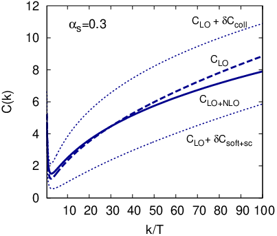
In the phenomenologically interesting momentum range, $k/T\sim 10$ , the collinear and semi-collinear+soft corrections largely cancel, leading to a small positive correction of order $\sim 15\%$ (Fig. 18(a)). At large momentum, $k/T{\ \lower-1.2pt\vbox{\hbox{\hbox to0.0pt{$>$\hss}\lower 6.0pt\vbox{\hbox{$\sim$}}}}\ }20$ , the LO and LO+NLO curves cross and the NLO correction turns negative (Fig. 18(b)). We believe that the large cancellations we observe are rather accidental, and one should thus consider the curves $C_{\mathrm{LO}}(k/T)+\delta C_{\mathrm{coll}}(k/T)$ and $C_{\mathrm{LO}}(k/T)+\delta C_{\mathrm{soft+sc}}(k/T)$ as upper and lower limits respectively of an “uncertainty estimate” of the NLO calculation.

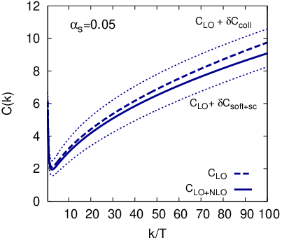
In Fig. 19 we plot $C_{\mathrm{LO+NLO}}(k/T)$ and $C_{\mathrm{LO}}(k/T)$ for $\alpha_{\mathrm{s}}=0.05$ , and $N_{c}=3$ , $N_{f}=3$ . For the smaller coupling constant the NLO correction is always negative and rather flat, and the magnitude of the two largely canceling contributions is also significantly smaller than in the previous case.

In Figs. 20 and 21 we plot the differential photon emission rates $d\Gamma_{\gamma}/dk$ relative to the leading order rate, (LO+ NLO)/LO, for two different values of the coupling constant. The reasonable, but somewhat ad hoc, “uncertainty estimate” described above can be inferred from the difference between the upper and lower dashed curves, which include either the collinear or the soft+semi-collinear correction, but not both.

For the largest coupling, $\alpha_{\mathrm{s}}=0.3$ , NLO corrections are modest and positive, although the “uncertainty band” is rather large – of order 50% (see Fig. 20). At intermediate coupling, $\alpha_{\mathrm{s}}=0.15$ , the cancellation between the collinear and semi-collinear+soft contributions is quite dramatic, causing the LO+NLO result to be within a few percent of the LO rate (not shown). Nevertheless, the uncertainty band remains rather large – of order $40\%$ . Finally, at the smallest coupling $\alpha_{\mathrm{s}}=0.05$ , the (LO+NLO)/LO ratio is somewhat larger than at intermediate coupling, but with a considerably smaller uncertainty band (Fig. 21).

7 Conclusions

We have computed the photon production rate to NLO of an equilibrated, weakly-coupled quark-gluon plasma. The contributions to the LO rate can be divided into distinct kinematical regimes — the hard, soft and collinear regions. The contributions arising from the hard and the soft regions have logarithmic sensitivity to the details of how the kinematical regions are divided. However, this dependence cancels in the sum. At NLO the soft and collinear regions receive ${\mathcal{O}}(g)$ corrections, and a new “semi-collinear” region starts to contribute here. We have dealt with the collinear region in Sec. 3, with the soft region in 4, and with the semi-collinear region in 5.

The collinear regime is affected by the LPM interference of multiple scatterings through the integral equation (18). As we showed, computations are most easily performed in impact parameter space and the resulting ${\mathcal{O}}(g)$ perturbation to the LO result is given in Eqs. (39). Furthermore two ${\mathcal{O}}(g)$ regions of the leading-order result, the soft region and the semi-collinear region, are identified and the asymptotic behaviors are derived in Eqs. (28) and (30). The treatment of these ${\mathcal{O}}(g)$ regions via the integral equation is incomplete, so we must recompute the contributions in these regions more carefully, subtracting off what has already been included in the collinear part of the calculation to avoid double counting.

In the soft region, we relied on the fact that causality dictates analyticity properties for the $n$ -point functions. Since the soft fields are lightlike separated as a result of the effective eikonalization of the hard fields, these analyticity properties lead to a tremendous simplification of the calculation: the soft bosonic correlators become the correlators of the 3D Euclidean theory, as pointed out in [21], whereas for fermions one can deform the integration contour of the non-vanishing light-cone momentum away from the real axis towards infinity, yielding a tractable expansion in inverse powers of that momentum. With these technical developments the soft contribution to the NLO rate is entirely analytic and given by Eq. (81), once the aforementioned subtraction of the collinear limit is performed. The result is incredibly simple: the NLO correction arising from the soft sector is the leading-order soft contribution modified by the shift $m_{\infty}^{2}\rightarrow m_{\infty}^{2}+\delta m_{\infty}^{2}$ , and nothing else. The contribution arising from the soft sector depends logarithmically on the UV regularization of the $p_{\perp}$ -integral; this dependence cancels against a corresponding IR divergence in the semi-collinear region.

In the semi-collinear region, the contribution from the soft gauge fields factorizes into a light-like separated, two-point correlator given by Eq. (85). This correlator is related to a momentum dependent transverse momentum diffusion coefficient experienced by a particle whose momentum obeys the semi-collinear scaling. We use again Euclidean techniques to evaluate it, obtaining a compact analytic result. Performing the remaining integrations (the last of which only numerically) and upon subtracting the appropriate ${\mathcal{O}}(g)$ regions of the leading-order result to avoid double countings, the contribution from the semi-collinear region is given by Eq. (92), which, as expected, shows an IR log divergence which combines with the soft contribution to make the final result finite and cutoff-independent.

In Sec. (6) we combine all contributions together in the full NLO rate and plot it for different values of the coupling. The striking feature is that the NLO correction is composed of two largely canceling contributions. The positive one arises from the collinear region and the negative one from the soft and semi-collinear regions. For $\alpha_{\mathrm{s}}=0.3$ , 3 colors and 3 light flavors, in the phenomenologically interesting momentum range, $k<15T$ , each contribution is a $50-75\%$ correction, but their sum is just a $10-20\%$ positive correction (see Fig. 18(a)). At higher momenta, the NLO correction turns negative, and the NLO+LO curve crosses the LO result (see Fig. 18(b)). For smaller values of the coupling, $\alpha_{\mathrm{s}}=0.05$ , the NLO correction is negative for all momenta (see Fig. 19).

For these reasons we believe this cancellation to be largely accidental, and thus consider the two separate contributions as the upper and lower bound of an uncertainty estimate for the NLO calculation. In Figs. 20 and 21 we plot the (LO+NLO)/LO ratio of photo-emission rates together with the uncertainty band for the two values of the coupling.

From the phenomenological point of view, the ${\mathcal{O}}(20\%)$ correction itself in the relevant region for $\alpha_{\mathrm{s}}=0.3$ does not alter qualitatively the current analyses [30]. On the other hand our ${\mathcal{O}}(100\%)$ uncertainty band gives a first estimate on the reliability of the perturbative calculation. Going to NNLO one would also encounter UV vacuum divergences and the associated running coupling, whose scale setting introduces another possibly large error band.

From the theoretical point of view, we believe that the main result of the present work lies in the developments related to the description of soft fields coupled to eikonalized hard fields. This progress opens new possibilities towards the calculation of other transport coefficients, such as the shear viscosity, at next-to-leading order. Furthermore, we believe the simple form of the NLO soft region can be understood more transparently in terms of an effective description of dipole propagation. Such a picture could also allow a factorization of the non-perturbative magnetic sector. We plan to return to these issues elsewhere.

A clear extension of this work would be the NLO treatment of gluon radiation, following the generalization from photon to gluon radiation at leading order in [31]. Other possible extensions include the calculation of the NLO rate in $\mathcal{N}=4$ SYM. The leading-order calculation at weak coupling was done in [32], together with the strong-coupling result. This could shed more light on the transition between the two regimes.

Analogously one could apply the methodologies we have developed to similar calculations for the thermal production of light-like particles, which could be of relevance for cosmology and whose rates are known only to leading order. Examples are ultrarelativistic right-handed neutrinos (see [29] for the LO rate), axions [33], saxions [34], axinos [35] and gravitinos [36].

Acknowledgments

We would like to thank Simon Caron-Huot, Yannis Burnier, and Peter Petreczky for useful conversations. We also thank the Institute for Nuclear Theory in Seattle, where some of this work was conducted. This work was supported in part by the Institute for Particle Physics (Canada) and the Natural Science and Engineering Research Council (NSERC) of Canada. DT is supported in part by an OJI grant from the US Department of Energy and the Sloan Foundation.

Appendix A Hard Thermal Loop propagators

In this section we detail our conventions for the HTL propagators. Fermion propagators are most easily written in terms of components with positive and negative chirality-to-helicity ratio. The retarded fermion propagator reads

S_{R}(P)=h^{+}_{\mathbf{p}}S^{+}_{R}(P)+h^{-}_{\mathbf{p}}S^{-}_{R}(p)\,,

(101)

where

S^{\pm}_{R}(P)=\frac{i}{p^{0}\mp(p+\Sigma^{\pm}(p^{0}/p))}=\left.\frac{i}{\displaystyle p^{0}\mp\left[p+\frac{m_{\infty}^{2}}{2p}\left(1-\frac{p^{0}\mp p}{2p}\ln\left(\frac{p^{0}+p}{p^{0}-p}\right)\right)\right]}\right|_{p^{0}=p^{0}+i\epsilon},

(102)

where the upper (lower) sign refers to the positive (negative) chirality-to-helicity component. The projectors are $h^{\pm}_{\mathbf{p}}\equiv(\gamma^{0}\mp\vec{\gamma}\cdot\hat{p})/2$ and $m_{\infty}^{2}=g^{2}C_{\scriptscriptstyle R}T^{2}/4$ is the fermionic asymptotic mass squared.

Gluons are described in the strict Coulomb gauge by

	$\displaystyle G^{00}_{R}(Q)$	$\displaystyle=$	$\displaystyle\frac{i}{\displaystyle q^{2}+m_{\scriptscriptstyle D}^{2}\left(1-\frac{q^{0}}{2q}\ln\frac{q^{0}+q+i\epsilon}{q^{0}-q+i\epsilon}\right)},$		(103)
	$\displaystyle G^{ij}_{R}(Q)$	$\displaystyle=$	$\displaystyle(\delta^{ij}-\hat{q}^{i}\hat{q}^{j})G^{T}_{R}(Q)=\left.\frac{i(\delta^{ij}-\hat{q}^{i}\hat{q}^{j})}{\displaystyle q_{0}^{2}-q^{2}-\frac{m_{\scriptscriptstyle D}^{2}}{2}\left(\frac{q_{0}^{2}}{q^{2}}-\left(\frac{q_{0}^{2}}{q^{2}}-1\right)\frac{q^{0}}{2q}\ln\frac{q^{0}{+}q}{q^{0}{-}q}\right)}\right\|_{q^{0}=q^{0}+i\epsilon}.$

The other components of the propagators in the $r,a$ basis can be obtained through Eq. (3).

Appendix B Gauge invariant condensates

During the calculation, we encounter several condensates that can be written as integrals of correlators separated by a spacelike or lightlike separation:

$\displaystyle Z_{g}$	$\displaystyle\equiv$	$\displaystyle\frac{1}{d_{\scriptscriptstyle A}}\left\langle v_{\mu}F^{\mu\rho}\frac{-1}{(v\cdot D)^{2}}v_{\nu}F^{\nu}_{\,\rho}\right\rangle$	(105)
	$\displaystyle=$	$\displaystyle\frac{-1}{d_{A}}\int_{0}^{\infty}dx^{+}\,x^{+}\langle\vphantom{\frac{1}{2}}v_{k\,\mu}F_{a}^{\mu\nu}(x^{+},0,0_{\perp})U^{ab}_{\scriptscriptstyle A}(x^{+},0,0_{\perp};0,0,0_{\perp})v_{k\,\rho}{F_{b}^{\rho}}_{\nu}(0)\rangle,$	(106)
$\displaystyle Z_{f}$	$\displaystyle\equiv$	$\displaystyle\frac{1}{2d_{\scriptscriptstyle R}}\left\langle\overline{\psi}\frac{\not{v}}{v\cdot D}\psi\right\rangle$	(107)
	$\displaystyle=$	$\displaystyle\frac{-i}{2d_{\scriptscriptstyle R}}\int_{0}^{\infty}dx^{+}\langle\overline{\psi}(x^{+},0,0_{\perp})\,\not{v}_{k}\,U_{\scriptscriptstyle R}(x^{+},0,0_{\perp};0,0,0_{\perp})\psi(0)\rangle$	(107)
$\displaystyle\frac{\hat{q}(\delta E)}{g^{2}C_{\scriptscriptstyle R}}$	$\displaystyle=$	$\displaystyle\int_{-\infty}^{\infty}dx^{+}\,e^{ix^{+}\delta E}\,\frac{1}{d_{\scriptscriptstyle A}}\langle v^{\mu}_{k}{F_{\mu}}^{\nu}(x^{+},0,0_{\perp})U_{\scriptscriptstyle A}(x^{+},0,0_{\perp};0,0,0_{\perp})v^{\rho}_{k}F_{\rho\nu}(0)\rangle,$	(108)
$\displaystyle{\mathcal{C}}(x_{\perp})$	$\displaystyle=$	$\displaystyle\lim_{x^{+}\rightarrow\infty}-(x^{+})^{-1}\log(W(x^{+},x_{\perp})),$	(109)
$\displaystyle\hskip-12.91663ptW(x^{+},x_{\perp})$	$\displaystyle\equiv$	$\displaystyle{\rm Tr}\>\Big\langle\,U_{\scriptscriptstyle R}(0,0,x_{\perp};x^{+},0,x_{\perp})\,U_{\scriptscriptstyle R}(0,0,0;0,0,x_{\perp})$	(110)
		$\displaystyle\qquad\,U_{\scriptscriptstyle R}(x^{+},0,0;0,0,0)\,U_{\scriptscriptstyle R}(x^{+},0,x_{\perp};x^{+},0,0)\Big\rangle\,.$	(110)

Here coordinates are written as triples $(x^{+},x^{-},x_{\perp})$ with $x^{-}=(t-z)$ and $x^{+}=(t+z)/2$ , so that $t=z=x^{+}$ when $x^{-}=0$ and $X\cdot P=x_{\perp}\cdot p_{\perp}-x^{-}p^{+}-x^{+}p^{-}$ . $U(x_{1};x_{2})$ is the Wilson line connecting the point $x_{1}$ to the point $x_{2}$ , in either the adjoint representation ( $U_{\scriptscriptstyle A}$ ) or the representation of the fermions ( $U_{\scriptscriptstyle R}$ ), and $W$ is the Wilson loop with a transverse segment of extent $x_{\perp}$ and a lightlike segment of extent $x^{+}$ in the $(t,z)$ directions [37]. For $Z_{g}$ and $Z_{f}$ we have employed rotational invariance and chosen the light-like vector $v$ to be $v_{k}$ without loss of generality.

The condensates $Z_{g}$ and $Z_{f}$ are related to the bosonic and fermionic hard thermal loops [38]. They describe how fluctuations in the gauge fields ( $Z_{g}$ ) and the fermionic fields ( $Z_{f}$ ) can influence the propagation of a fermion moving through the plasma at nearly the speed of light. Therefore they determine the dispersion correction of hard $p^{+}\gg gT$ excitations; they are valid both at leading and at next-to-leading order [22]. And ${\mathcal{C}}(x_{\perp})$ and $\frac{\hat{q}(\delta E)}{g^{2}C_{\scriptscriptstyle R}}$ are related to the scattering processes in the medium; ${\mathcal{C}}(x_{\perp})$ arises when treating collinear splitting and is discussed in Sec. 3, while $\frac{\hat{q}(\delta E)}{g^{2}C_{\scriptscriptstyle R}}$ arises when treating the semi-collinear regime, in Eq. (85). They are related;

\lim_{x_{\perp}\rightarrow 0}\partial^{2}_{x_{\perp}}{\mathcal{C}}(x_{\perp})=\lim_{\delta E\rightarrow 0}\hat{q}(\delta E)\,.

(111)

In this appendix we show how these condensates are most conveniently computed by using Euclidean methods developed in [21]. But first let us set up their calculation via real-time techniques, so we can see how expressions, encountered in the main text, do indeed correspond to these condensates. Except for ${\mathcal{C}}(x_{\perp})$ , we only encounter the condensates at lowest order, where the Wilson line is set to unity and the field strengths take their abelian form. Working to this order, consider first $Z_{g}$ . Recall that

	$\displaystyle\langle F_{\mu\nu}(X)F_{\alpha\beta}(0)\rangle$	$\displaystyle=$	$\displaystyle\int\frac{d^{4}Q}{(2\pi)^{4}}\>e^{iQ\cdot X}\Big(Q_{\mu}Q_{\alpha}G^{>}_{\nu\beta}(Q)-Q_{\nu}Q_{\alpha}G^{>}_{\mu\beta}(Q)$		(112)
			$\displaystyle\hskip 77.49976pt-Q_{\mu}Q_{\beta}G^{>}_{\nu\alpha}(Q)+Q_{\nu}Q_{\beta}G^{>}_{\mu\alpha}(Q)\Big)\,.$		(112)

Applying this to Eq. (106) and performing the $x^{-}$ integral, one finds (ignoring the difference between $G^{>}$ and $G_{rr}$ , which is higher order in the soft region)

Z_{g}=\int\frac{d^{2}q_{\perp}\,dq^{+}dq^{-}}{(2\pi)^{4}}\left[\frac{q_{\perp}^{2}G^{++}_{rr}(Q)}{(q^{-}-i\epsilon)^{2}}-2\frac{q_{z}G_{T}^{rr}(Q)}{(q^{-}-i\epsilon)}\left(1{-}\frac{q_{z}^{2}}{q^{2}}\right)+G_{T}^{rr}(Q)\left(1+\frac{q_{z}^{2}}{q^{2}}\right)\right]\,.

(113)

This is the same as the expression encountered in the “soft part” of the calculation, Eq. (77), except that there the leading-order behavior is to be subtracted.

The calculation of $\hat{q}(\delta E)$ is analogous, except that the $x^{+}$ integral produces a delta function fixing $q^{-}$ :

\frac{\hat{q}(\delta E)}{g^{2}C_{\scriptscriptstyle R}}=\int\frac{d^{4}Q}{(2\pi)^{3}}\delta(q^{-}-\delta E)\left[q_{\perp}^{2}G^{++}_{rr}(Q)+G_{T}^{rr}(Q)\left(\left[1{+}\frac{q_{z}^{2}}{q^{2}}\right]\delta E^{2}-2q_{z}\delta E\left[1{-}\frac{q_{z}^{2}}{q^{2}}\right]\right)\right].

(114)

This is identical to Eq. (85).

It would be possible to compute these Minkowski-domain expressions explicitly using the sum rule approach; but we find it simpler and more instructive to compute them via Euclidean techniques.

B.1 Relation to Euclidean functions: Simple derivation

Caron-Huot has shown that $n$ -point correlation functions, where all fields lie on a spacelike hypersurface, can be carried out by Euclidean techniques [21]. The null correlators we need can also be computed provided that they are free of collinear singularities, which they are. The proof presented in Ref. [21] is rather complex and technical. Here we will present a much simpler derivation, also due to Caron-Huot¹³¹³ 13 S. Caron-Huot, oral presentation at the Institute for Nuclear Theory (Seattle), 29 March 2012, which works for two point functions. In practice this is all we need, except for the NLO evaluation of ${\mathcal{C}}(x_{\perp})$ .

Consider the ordering-averaged correlator of some operator (such as the field strength), $G_{rr}(x^{0},{\bf{x}})$ with $|x^{z}|>|x^{0}|$ . (Since the separation is spacelike, operators commute, and therefore $G_{rr}$ equals $G^{<}$ , $G_{\scriptscriptstyle F}$ , or $G^{>}$ .) Write it in terms of its Fourier representation

G_{rr}(x^{0},{\bf{x}})=\int d\omega\int dp_{z}d^{2}p_{\perp}e^{i(x^{z}p^{z}+\mathbf{x}_{\perp}\cdot\mathbf{p}_{\perp}-\omega x^{0})}\>G_{rr}(\omega,p_{z},p_{\perp}),

(115)

and use

G_{rr}(\omega,p)=\left(n_{\!\scriptscriptstyle B}(\omega)+\frac{1}{2}\right)\left(G_{R}(\omega,p)-G_{A}(\omega,p)\right)=\left(n_{\!\scriptscriptstyle B}(\omega)+\frac{1}{2}\right)\rho(\omega,p),

(116)

and define $\tilde{p}^{z}=p^{z}-(t/x^{z})\omega$ :

G_{rr}(x^{0},{\bf{x}})=\int d\omega\int d\tilde{p}_{z}d^{2}p_{\perp}e^{i(x^{z}\tilde{p}^{z}+\mathbf{x}_{\perp}\cdot\mathbf{p}_{\perp})}\left(n_{\!\scriptscriptstyle B}(\omega)+\frac{1}{2}\right)\>\rho(\omega,\tilde{p}+\omega(x^{0}/x^{z}),p_{\perp})\,.

(117)

Now we perform the $\omega$ integration by contour methods. The retarded function in $\rho(\omega,p)$ is related to the Euclidean function via $G_{R}(\omega,p)=-iG_{E}(i\omega,p)$ , that is, by analytic continuation. This continuation is guaranteed not to encounter singularities in the Green function so long as the imaginary part of the 4-momentum remains timelike – since then, in some frame, the continuation is purely of the frequency. Since $|x^{0}/x^{z}|<1$ , the continuation of $G_{R}(\omega,\tilde{p}-\omega(x^{0}/x^{z}),p_{\perp})$ in $\omega$ will not encounter any singularity in the upper complex $\omega$ plane. The advanced function similarly will be free of singularities in the lower plane. Therefore the only singularities encountered in continuing the frequency integration are those in the statistical function $(n_{\!\scriptscriptstyle B}(\omega)+1/2)$ , which has poles at $\omega=2\pi inT$ with $n=(\ldots-1,0,1,\ldots)$ and residue equal to $T$ . Closing the contour around these poles, and renaming $\tilde{p}^{z}$ to $p^{z}$ , we find¹⁴¹⁴ 14 The pole at $n=0$ is an artifact of the separation of $\rho$ , which vanishes for $\omega=0$ , into $G_{R}$ and $G_{A}$ . The individual poles there can then be dealt with in a principal value prescription, for instance.

G_{rr}(x^{0},x^{z},x_{\perp})=T\sum_{n}\int\frac{d^{3}p}{(2\pi)^{3}}e^{i(x^{z}p^{z}+\mathbf{x}_{\perp}\cdot\mathbf{p}_{\perp})}G_{E}(\omega_{n},p_{z}+i\omega_{n}(x^{0}/x^{z}),p_{\perp})\,,\quad\omega_{n}=2\pi nT\,.

(118)

In any case where we need to compute the soft $gT$ contribution to such a correlator, one may drop the nonzero Matsubara frequency contributions; that is, we keep only the $n=0$ term in the sum. For this term, $G_{E}(\omega_{n},p_{z}+i\omega_{n}(x^{0}/x^{z}),p_{\perp})=G_{E}(0,p_{z},p_{\perp})$ is the Euclidean correlation function of the 3-dimensional dimensionally reduced (Electric QCD or EQCD) theory. [EQCD is the 3D theory consisting of the spatial gauge fields $A_{i}$ and an adjoint scalar descended from the temporal component of the gauge field, $\Phi=iA_{0}$ . The scalar is massive, $m^{2}_{\Phi}=m_{\scriptscriptstyle D}^{2}$ ; see for instance [39].]

B.2 Application to Scattering

First we apply this method to determine ${\mathcal{C}}(q_{\perp})$ and $\hat{q}(\delta E)$ at leading order. There,

{\mathcal{C}}_{\rm LO}(q_{\perp})=g^{2}C_{\scriptscriptstyle R}\int dx^{+}\int d^{2}x_{\perp}e^{-i\mathbf{q}_{\perp}\cdot\mathbf{x}_{\perp}}G^{++}_{rr}(x^{+},0,x_{\perp})\,,

(119)

where this position space expression makes clear that we are dealing with a spacelike separation and hence Eq. (118) is applicable, yielding

	$\displaystyle{\mathcal{C}}_{\rm LO}(q_{\perp})$	$\displaystyle=$	$\displaystyle g^{2}C_{\scriptscriptstyle R}T\sum_{n}\int\frac{d^{3}p}{(2\pi)^{3}}G^{++}_{E}(p_{n}^{0},p_{n}^{z},p_{\perp})(2\pi)^{3}\delta(p_{z})\delta^{2}(\mathbf{p}_{\perp}-\mathbf{q}_{\perp})$		(120)
		$\displaystyle=$	$\displaystyle g^{2}C_{\scriptscriptstyle R}T\left(\frac{1}{q_{\perp}^{2}}-\frac{1}{q_{\perp}^{2}+m_{\scriptscriptstyle D}^{2}}\right)+\mbox{hard ($n\neq 0$) contributions}\,.$		(120)

The $1/q_{\perp}^{2}$ and $1/(q_{\perp}^{2}+m_{\scriptscriptstyle D}^{2})$ terms are the contributions from the $A_{z}A_{z}$ correlator and the $A_{0}A_{0}$ correlator respectively. The nonzero Matsubara frequency contributions are suppressed, for $q_{\perp}\sim gT$ , by a power of $g^{2}$ and may be neglected. This result was first found by Aurenche Gelis and Zaraket [26], by a rather more complicated sum rule procedure, which involved canceling $1/(q_{\perp}^{2}+m_{\scriptscriptstyle D}^{2}/3)$ poles. The current procedure, originally due to Caron-Huot [21], avoids this complication.

With this Euclidean framework the NLO (1-loop) corrections also become tractable as a computation within dimensionally-reduced EQCD [21]. We will return to this result in the next appendix.

Next consider $\hat{q}(\delta E)$ , Eq. (108). We work to lowest order, replacing the Wilson line with the identity and keeping only the two-point correlator of the $A$ -fields in the field strengths. We may again apply Eq. (118) and to find the infrared contribution we may keep only the $n=0$ term. This corresponds to the replacements $G_{rr}\to G_{E}$ , $\int dq^{0}/(2\pi)\to T$ and $q^{0}\to 2\pi inT\to 0$ , $q^{+}\to q_{z}$ . Writing the gauge field correlator in terms of its momentum space representation, we then obtain

$\displaystyle\frac{\hat{q}(\delta E)}{g^{2}C_{\scriptscriptstyle R}}$	$\displaystyle=$	$\displaystyle T\int\frac{d^{3}q}{(2\pi)^{3}}\left[q_{\perp}^{2}G^{++}_{E}(0,q_{z},q_{\perp})+G_{T}^{E}(0,q_{z},q_{\perp})\left(\left[1{+}\frac{q_{z}^{2}}{q^{2}}\right]\delta E^{2}-2q_{z}\delta E\left[1{-}\frac{q_{z}^{2}}{q^{2}}\right]\right)\right]$	(121)
		$\displaystyle\hskip 62.59596pt\times 2\pi\delta(q_{z}+\delta E)$
	$\displaystyle=$	$\displaystyle T\int\frac{d^{2}q_{\perp}}{(2\pi)^{2}}\left[\frac{m_{\scriptscriptstyle D}^{2}q_{\perp}^{2}}{(q_{\perp}^{2}+\delta E^{2})(q_{\perp}^{2}+\delta E^{2}+m_{\scriptscriptstyle D}^{2})}+\frac{2\delta E^{2}}{q_{\perp}^{2}+\delta E^{2}}\right].$

B.3 Application to $\delta Z_{g}$

Let us now apply the Euclidean formalism to compute $Z_{g}$ at NLO. Our starting point will be the position space expression of Eq. (106). Since the positions involved are lightlike separated, we may apply Eq. (118).

The leading order contribution to $Z_{g}$ arises from hard $p^{+}\sim T$ excitations; it therefore arises from a range of $n$ values and is not easily established by Euclidean methods. However the leading order value is easy to determine by conventional methods, and equals

Z_{g}^{\rm LO}=2\int\frac{d^{3}p}{(2\pi)^{3}p}n_{\!\scriptscriptstyle B}(p)=\frac{T^{2}}{6}.

(122)

For $n\neq 0$ the correlation functions receive ${\mathcal{O}}(g^{2})$ loop corrections, so any corrections from $n\neq 0$ are ${\mathcal{O}}(g^{2})$ and therefore beyond our current precision goal. To find the ${\mathcal{O}}(g)$ NLO corrections, we need to compute the contribution from $n=0$ modes and subtract the leading-order, unresummed-theory value. A straightforward evaluation of Eq. (106), replacing $x^{+}$ with $x_{z}$ and using 3-dimensional Euclidean correlation functions, gives

\delta Z_{g}=T\!\int\!\frac{d^{3}q}{(2\pi)^{3}}\!\left[\frac{q_{\perp}^{2}G_{E}^{++}(0,q_{z},q_{\perp})}{(q_{z}+i\epsilon)^{2}}+G_{T}^{E}(0,q_{z},q_{\perp})\left(3-\frac{q_{z}^{2}}{q^{2}}\right)-\mbox{ same, free propagators}\right],

(123)

where the $i\epsilon$ prescription in $1/(q_{z}+i\epsilon)^{2}$ arises from the boundary conditions on the $z$ integration, $\int_{0}^{\infty}zdz$ . Now the bare and interacting $A_{i}$ correlators are the same at leading order, but the temporal mode $A_{0}$ develops a (Debye) mass; $\langle A_{0}A_{0}(q)=\frac{-1}{q^{2}+m_{\scriptscriptstyle D}^{2}}$ whereas the bare value is $-1/q^{2}$ . (The minus sign is because there is an $i$ difference between the Minkowski and Euclidean $A^{0}$ field, so $A^{+}=A^{z}+iA^{0}$ .) Therefore only the $G_{E}^{00}$ part of the first term is not canceled by the relevant free version. Its subtracted contribution is then

\delta Z_{g}=T\int\frac{d^{3}q}{(2\pi)^{3}}\frac{q_{\perp}^{2}}{(q_{z}+i\epsilon)^{2}}\left(\frac{-1}{q^{2}+m_{\scriptscriptstyle D}^{2}}+\frac{1}{q^{2}}\right)=-\frac{Tm_{\scriptscriptstyle D}}{2\pi}.

(124)

The correction is ${\mathcal{O}}(g)$ relative to Eq. (122) and negative, representing a reduction in the thermal mass due to the screening of infrared gauge modes.

No such ${\mathcal{O}}(g)$ correction arises for $Z_{f}$ because the correlator directly involves fermionic fields which do not have zero modes. To ${\mathcal{O}}(g)$ accuracy,

Z_{f}=2\int\frac{d^{3}p}{(2\pi)^{3}p}n_{\!\scriptscriptstyle F}(p)=\frac{T^{2}}{12}\,.

(125)

B.4 Thermal mass at NLO

We now apply these results for $Z_{g}$ and $Z_{f}$ to the fermionic effective mass. The thermal dispersion relation for a particle approaches $p_{0}^{2}=p^{2}+m_{\infty}^{2}$ for $p^{0}\approx p\gg gT$ , where $m_{\infty}^{2}$ is the asymptotic mass. The asymptotic mass is given by the real part of the fermion self-energy. In more detail we have [40]

m_{\infty}^{2}=2p\,\mathrm{Re}\,\Sigma_{R}^{+}(p^{0}=p)\,,\qquad\Sigma_{R}^{+}(P)\equiv\frac{1}{2}\textrm{Tr}\left[h^{+}_{p}\Sigma_{R}(P)\right].

(126)

To the order of interest, one diagram contributes to the retarded self-energy, see Fig. 22. There are two $r,a$ assignments; either the fermion is retarded and the gluon is $rr$ , or the gluon is retarded and the fermion is $rr$ . The retarded line, which in the NLO calculation always carries a large momentum, enforces the eikonality; the operator correlation in $Z_{g}$ ( $Z_{f}$ ) corresponds to the cut gauge boson (fermion) line. One easily finds that [22]

m_{\infty}^{2}=g^{2}C_{\scriptscriptstyle R}(Z_{g}+Z_{f})\,.

(127)

We just found that, at NLO, the condensates read [22]

	$\displaystyle Z_{g}$	$\displaystyle=$	$\displaystyle Z_{g}^{\rm{LO}}+\delta Z_{g},\quad Z_{g}^{\rm{LO}}=\frac{T^{2}}{6},\quad\delta Z_{g}=-\frac{Tm_{\scriptscriptstyle D}}{2\pi}\,,$		(128)
	$\displaystyle Z_{f}$	$\displaystyle=$	$\displaystyle Z_{f}^{LO}+\delta Z_{f},\quad Z_{f}^{LO}=\frac{T^{2}}{12},\quad\delta Z_{f}=0\,,$		(129)

which, together with the well known result for the leading order Debye mass

m_{\scriptscriptstyle D}^{2}=\frac{g^{2}}{3}(C_{\scriptscriptstyle A}+T_{R}N_{f})T^{2}\,,

(130)

yields the fermionic $m_{\infty}^{2}$ at NLO in QCD,¹⁵¹⁵ 15 In [40] the asymptotic mass was computed numerically at NLO in the large- $N_{f}$ non-abelian theory. The authors found a strong momentum dependence of their NLO result, in sharp contrast with Eq. (131), which however reproduces their average shift. It is our understanding that, in the context of a strict $g$ expansion, the result of Caron-Huot [22] is correct for fermion momenta much larger than $gT$ .

m^{2}_{\infty,\rm NLO}=m_{\infty}^{2}+\delta m_{\infty}^{2}=g^{2}C_{\scriptscriptstyle R}\left(\frac{T^{2}}{4}-\frac{gT^{2}}{2\pi}\sqrt{\frac{2N_{c}+N_{f}}{6}}\right).

(131)

Appendix C NLO collision kernel

In the previous appendix we presented the definition of the differential collision rate ${\mathcal{C}}(x_{\perp})$ and found its leading order expression in transverse momentum space, ${\mathcal{C}}(q_{\perp})$ . Its NLO expression in $q_{\perp}$ space has also been found [22]; writing ${\mathcal{C}}_{\textrm{NLO}}={\mathcal{C}}+\delta{\mathcal{C}}$ , explicitly

$\displaystyle\delta{\mathcal{C}}(q_{\perp})$	$\displaystyle\!=\!$	$\displaystyle(g^{4}T^{2}C_{\scriptscriptstyle R}C_{\scriptscriptstyle A})\left[-\frac{m_{\scriptscriptstyle D}{+}2\frac{q_{\perp}^{2}-m_{\scriptscriptstyle D}^{2}}{q_{\perp}}\arctan\frac{q_{\perp}}{m_{\scriptscriptstyle D}}}{4\pi(q_{\perp}^{2}{+}m_{\scriptscriptstyle D}^{2})^{2}}+\frac{m_{\scriptscriptstyle D}-\frac{q_{\perp}^{2}{+}4m_{\scriptscriptstyle D}^{2}}{2q_{\perp}}\arctan\frac{q_{\perp}}{2m_{\scriptscriptstyle D}}}{8\pi q_{\perp}^{4}}\right.$	(132)
		$\displaystyle\hskip 85.35826pt-\frac{\arctan\frac{q_{\perp}}{m_{\scriptscriptstyle D}}}{2\pi q_{\perp}(q_{\perp}^{2}{+}m_{\scriptscriptstyle D}^{2})}+\frac{\arctan\frac{q_{\perp}}{2m_{\scriptscriptstyle D}}}{2\pi q_{\perp}^{3}}+\frac{7}{32q_{\perp}^{3}}$
		$\displaystyle\hskip 85.35826pt\left.+\frac{m_{\scriptscriptstyle D}}{4\pi(q_{\perp}^{2}{+}m_{\scriptscriptstyle D}^{2})}\left(\frac{3}{q_{\perp}^{2}{+}4m_{\scriptscriptstyle D}^{2}}-\frac{2}{q_{\perp}^{2}{+}m_{\scriptscriptstyle D}^{2}}-\frac{1}{q_{\perp}^{2}}\right)\!\right].$

In order to use the collision kernel in Eq. (33), we need to Fourier transform this expression to find ${\mathcal{C}}^{\prime}(b)$ , preferably analytically but at minimum via accurate numerical integration.

The integral at leading order can be performed by taking partial fractions and considering $e^{i{\bf{b}}\cdot{\bf{q}}_{\perp}}/(q_{\perp}^{2}+m_{\scriptscriptstyle D}^{2})$ :

			$\displaystyle\int_{-\infty}^{\infty}\frac{dq_{1}}{2\pi}e^{ibq_{1}}\int_{-\infty}^{\infty}\frac{dq_{2}}{2\pi}\frac{1}{q_{2}^{2}+q_{1}^{2}+m_{\scriptscriptstyle D}^{2}}=\int_{-\infty}^{\infty}\frac{dq_{1}}{2\pi}e^{ibq_{1}}\frac{1}{2\sqrt{q_{1}^{2}+m_{\scriptscriptstyle D}^{2}}}$		(133)
		$\displaystyle=$	$\displaystyle\frac{1}{2\pi}\int_{m_{\scriptscriptstyle D}}^{\infty}\frac{dx}{\sqrt{x^{2}-m_{\scriptscriptstyle D}^{2}}}e^{-bx}=\frac{K_{0}(bm_{\scriptscriptstyle D})}{2\pi}\,,$		(133)

where, after performing the trivial $q_{2}$ integration, we changed contours to pick up the discontinuity along the cut of the $\sqrt{q^{2}+m_{\scriptscriptstyle D}^{2}}$ function; $x\equiv{\rm Im}\,q$ . Ultimately we need the same expression with $m_{\scriptscriptstyle D}\rightarrow 0$ , and with $b\rightarrow 0$ for each (finite and zero $m_{\scriptscriptstyle D}$ ) case;

$\displaystyle{\mathcal{C}}^{\prime}(b)$	$\displaystyle\equiv$	$\displaystyle\int\frac{d^{2}q_{\perp}}{(2\pi)^{2}}\Big(1-e^{i{\bf{b}}\cdot{\bf{q}}_{\perp}}\Big){\mathcal{C}}(q_{\perp}){\mathcal{C}}_{\rm LO}^{\prime}(b)$
	$\displaystyle=$	$\displaystyle g^{2}TC_{\scriptscriptstyle R}\lim_{\epsilon\rightarrow 0}\frac{1}{2\pi}\left(K_{0}(\epsilon b\epsilon m_{\scriptscriptstyle D})-K_{0}(b\epsilon m_{\scriptscriptstyle D})-K_{0}(\epsilon bm_{\scriptscriptstyle D})+K_{0}(bm_{\scriptscriptstyle D})\right)\,,$
$\displaystyle\frac{{\mathcal{C}}_{\rm LO}^{\prime}(b)}{g^{2}TC_{\scriptscriptstyle R}}$	$\displaystyle=$	$\displaystyle\frac{1}{2\pi}\left(K_{0}(bm_{\scriptscriptstyle D})+\gamma_{\rm E}+\ln(bm_{\scriptscriptstyle D}/2)\right)\,.$	(134)

We follow the same strategy for the terms in the NLO correction (132). We first perform the $q_{2}$ integration (the direction orthogonal to ${\bf{b}}$ ). This can generally be done by deforming the contour to pick up all poles and cuts. In every case the resulting integral can be done analytically. Then we perform the $q_{1}$ integration. In some cases this can be done analytically, in other cases the $b=0$ case is analytic but the finite $b$ case involves an integral along a cut. Finally there are cases where the difference, $1-e^{-bx}$ must be integrated along a cut. Some of these integrals remain numerical, but all converge exponentially and are small for large $b$ .

Without going into detail, the result (writing the terms in the same order as they appear in Eq. (132)) is

	$\displaystyle\frac{m_{\scriptscriptstyle D}\,\delta{\mathcal{C}}^{\prime}(b)}{g^{4}T^{2}C_{\scriptscriptstyle R}C_{\scriptscriptstyle A}}$	(135)
$\displaystyle=$	$\displaystyle-\frac{1}{8\pi^{2}}\left[\frac{bm_{\scriptscriptstyle D}K_{1}(bm_{\scriptscriptstyle D})-1+4-4e^{-bm_{\scriptscriptstyle D}}}{2}+\int_{1}^{\infty}dz\left(e^{-bm_{\scriptscriptstyle D}}-e^{-bm_{\scriptscriptstyle D}z}\right)\frac{\ln\frac{z^{2}}{z^{2}-1}}{(z^{2}-1)^{3/2}}\right]$
	$\displaystyle{}-\frac{1}{96\pi^{2}}\int_{0}^{\infty}\frac{dz}{z}(1-e^{-bm_{\scriptscriptstyle D}z})\left(1-\frac{(z^{2}-4)^{3/2}\theta(z-2)}{z^{3}}\right)$
	$\displaystyle-\frac{1}{32}+\frac{1}{8\pi^{2}}\int_{1}^{\infty}\!\!dz\frac{e^{-bm_{\scriptscriptstyle D}z}\ln\frac{z^{2}}{z^{2}-1}}{\sqrt{z^{2}-1}}{}+\frac{1}{8\pi^{2}}\int_{0}^{\infty}\frac{dz}{z}\left(1-e^{-bm_{\scriptscriptstyle D}z}\right)\left(1-\frac{\theta(z{-}2)\sqrt{z^{2}{-}4}}{z}\right)$
	$\displaystyle{}+\frac{7bm_{\scriptscriptstyle D}}{64\pi}+\frac{1}{8\pi^{2}}\Big[K_{0}(2bm_{\scriptscriptstyle D})-2K_{0}(bm_{\scriptscriptstyle D})+\ln\frac{4}{m_{\scriptscriptstyle D}b}-\gamma_{\rm E}+bm_{\scriptscriptstyle D}K_{1}(bm_{\scriptscriptstyle D})-1\Big]\,.$

We have been unable to perform these integrals analytically. However, they are quite straightforward numerically, and they also have a simple behavior in the large $bm_{\scriptscriptstyle D}$ limit:

\frac{m_{\scriptscriptstyle D}\,\delta{\mathcal{C}}^{\prime}(b)}{g^{4}T^{2}C_{\scriptscriptstyle R}C_{\scriptscriptstyle A}}\xrightarrow[bm_{\scriptscriptstyle D}\gg 1]{}\frac{7bm_{\scriptscriptstyle D}}{64\pi}+\frac{-9\pi^{2}-58+72\ln(2)-3(\ln(bm_{\scriptscriptstyle D})+\gamma_{\rm E})}{288\pi^{2}}+{\mathcal{O}}(\exp(-bm_{\scriptscriptstyle D})).

(136)

This has the interpretation as the total scattering rate, IR regulated at a scale $q\sim 1/b$ . While the leading order total scattering rate has a logarithmic divergence, the NLO has a linear divergence. Note that the corrections to this linear + constant + log behavior are exponentially suppressed.

The small $bm_{\scriptscriptstyle D}$ behavior is

\displaystyle\frac{m_{\scriptscriptstyle D}\,\delta{\mathcal{C}}^{\prime}(b)}{g^{4}T^{2}C_{\scriptscriptstyle R}C_{\scriptscriptstyle A}}\xrightarrow[bm_{\scriptscriptstyle D}\gg 1]{}\frac{-bm_{\scriptscriptstyle D}}{32\pi}+\frac{\hat{q}_{\rm nlo}b^{2}m_{\scriptscriptstyle D}^{2}}{4}+{\cal O}(b^{3})\,,\quad\hat{q}_{\rm nlo}\!\!=\!\!

\displaystyle\frac{3\pi^{2}+10-4\ln(2)}{32\pi^{2}}\,.

(137)

Here $\hat{q}_{\rm nlo}$ is the NLO correction to the momentum broadening rate. To see this, expand Eq. (34) in small $b$ and angle average, $\exp(i{\bf{b}}\cdot{\bf{q}}_{\perp})\sim 1-({\bf{b}}\cdot{\bf{q}}_{\perp})^{2}/2\sim 1-b^{2}q^{2}/4$ . The integral $\int d^{2}q\;q^{2}{\mathcal{C}}(q)$ is what we usually mean by $\hat{q}$ ; hence $\hat{q}_{\rm nlo}$ is the numerical coefficient on the NLO contribution to $\hat{q}$ . We have thus verified that the expansion performed on the expression in Eq. (135) reproduces the expected linear-in- $b$ and $\hat{q}$ behavior found by Caron-Huot [21].

Note that the small $b$ behavior is actually negative. Our understanding is that this is actually correct. Basically, small $b$ corresponds to large momentum transfers, a limit where our treatment of exchange momenta as $gT\ll T$ breaks down. In [21], Caron-Huot showed how an opposite term arises in the soft limit of the hard contribution to $\hat{q}$ , leading to a cancellation. Had we used dimensional regularization to perform the integration of $b^{2}q^{2}{\mathcal{C}}_{\mathrm{NLO}}(q)/4$ , the linear term would simply have vanished.

Appendix D Evaluation of the semi-collinear integrations

In this Appendix we evaluate numerically the integrals appearing in Eq. (). In order to match properly with the UV divergence in the soft region, which was regulated by a cutoff $\mu_{\perp}^{\mathrm{NLO}}$ ( $gT\ll\mu_{\perp}^{\mathrm{NLO}}\ll\sqrt{g}T$ ) in the transverse momentum $p_{\perp}$ , we regulate the IR region with the same transverse cutoff. As we mentioned, we split the calculation into a bremsstrahlung/Compton contribution ( $p^{+}>0$ ) and an annihilation contribution ( $-k/2<p^{+}<0$ ), where we used the symmetry under $p^{+}\to-p^{+}-k$ . We start with the former.

D.1 The bremsstrahlung/Compton contribution: $\Gamma_{{\mathrm{semi-coll}}}^{\rm brem/Compt.}$

As we shall show, it is technically convenient to first introduce an intermediate regulator $\mu^{+}$ for the $dp^{+}$ integration, with $gT\ll\mu^{+}\ll T$ , hence $\mu^{+}\gg\mu_{\perp}^{\mathrm{NLO}}$ . In practice we divide the phase space in two regions, i.e.

1.

First we take $p^{+}>\mu^{+}$ , $p_{\perp}>\mu_{\perp}^{\mathrm{NLO}}$ .
2.

We then consider the slice $0<p^{+}<\mu^{+}$ , $p_{\perp}>\mu_{\perp}^{\mathrm{NLO}}$ , where only the IR asymptotic behavior in $p^{+}$ needs to be considered.

The dependence on $\mu^{+}$ cancels in the sum of the two regions.

The $p_{\perp}$ and $q_{\perp}$ integrations on the second line of Eq. () yield

	$\displaystyle\frac{1}{2\pi}\int_{\mu_{\perp}^{\mathrm{NLO}}}^{\infty}\frac{dp_{\perp}\,p_{\perp}}{\delta E^{2}}\int\frac{d^{2}q_{\perp}}{(2\pi)^{2}}\left[\frac{m_{\scriptscriptstyle D}^{2}q_{\perp}^{2}}{(q_{\perp}^{2}+\delta E^{2})(q_{\perp}^{2}+\delta E^{2}+m_{\scriptscriptstyle D}^{2})}-\frac{m_{\scriptscriptstyle D}^{2}}{q_{\perp}^{2}+m_{\scriptscriptstyle D}^{2}}\right]$
	$\displaystyle=-\frac{m_{\scriptscriptstyle D}}{4\pi k}\|p^{+}(k+p^{+})\|+\mathcal{O}\left((\mu_{\perp}^{\mathrm{NLO}})^{2}\right),$		(138)

where we have used the fact that $p^{+}\gg\mu_{\perp}^{\mathrm{NLO}}$ . The first term on the second line is the result one would obtain with vanishing cutoff. As we mentioned in the previous section, matching regions for momenta of the order of the cutoffs are equally described by the regions on either side of it and the dependence on the cutoff has to vanish at all orders. Power-law terms can then be neglected and we can just plug the first term in Eq. (), yielding

(2\pi)^{3}\frac{d\Gamma_{\gamma}}{d^{3}k}\bigg|_{\mathrm{brem/compton}}^{(1)}=-\frac{m_{\scriptscriptstyle D}}{\pi T}\mathcal{A}(k)\int_{\mu^{+}}^{\infty}dp^{+}\frac{n_{\!\scriptscriptstyle F}(k+p^{+})(1-n_{\!\scriptscriptstyle F}(p^{+}))}{n_{\!\scriptscriptstyle F}(k)}\frac{(k+p^{+})^{2}+(p^{+})^{2}}{k\,p^{+}\,(p^{+}+k)}.

(139)

This expression is IR log divergent. The logarithm can be extracted by adding and subtracting $\theta(T-p^{+})/(2p^{+})$ under the integral sign, so that

-\frac{m_{\scriptscriptstyle D}}{\pi T}\mathcal{A}(k)\int_{\mu^{+}}^{T}dp^{+}\frac{1}{2p^{+}}=-\frac{m_{\scriptscriptstyle D}}{2\pi T}\mathcal{A}(k)\ln\frac{T}{\mu^{+}},

(140)

and

(2\pi)^{3}\frac{d\Gamma_{\gamma}}{d^{3}k}\bigg|_{\mathrm{brem/compton}}^{(1)}=-\frac{m_{\scriptscriptstyle D}}{2\pi T}\mathcal{A}(k)\left[\ln\left(\frac{T}{\mu^{+}}\right)+C_{\mathrm{brem/compton}}\left(\frac{k}{T}\right)\right].

(141)

$C_{\mathrm{brem/compton}}(k/T)$ is defined as

	$\displaystyle C_{\mathrm{brem/compton}}\left(\frac{k}{T}\right)$	$\displaystyle=$	$\displaystyle 2\int_{0}^{\infty}dp^{+}\left[\frac{n_{\!\scriptscriptstyle F}(k+p^{+})(1-n_{\!\scriptscriptstyle F}(p^{+}))}{n_{\!\scriptscriptstyle F}(k)}\frac{(k+p^{+})^{2}+(p^{+})^{2}}{k\,p^{+}\,(p^{+}+k)}\right.$		(142)
			$\displaystyle\hskip 193.47882pt\left.-\frac{\theta(T-p^{+})}{2p^{+}}\right],$		(142)

where we stretch the integral to $0$ since it is now finite, the difference being given by negligible positive powers of $\mu^{+}/T$ . For further convenience, we parametrize $C_{\mathrm{brem/compton}}(k/T)$ with an accuracy of $2\%$ or better as

C_{\mathrm{brem/compton}}(x)=\frac{4-\ln(4)-\frac{\pi^{2}}{6}}{x}\sum_{n=1}^{4}d_{n}e^{-nx}+\left(-0.12563+\frac{\ln(4)}{x}+\frac{\pi^{2}}{6}\frac{1}{x^{2}+x}\right),

(143)

with

[d_{1}\ldots d_{4}]=[2.29467534576455,-3.0183977101591,1.2374580732449,0.486264291149683].

(144)

Let us now turn to region 2. By imposing the cutoffs and expanding for $p^{+}\ll k$ we have

	$\displaystyle(2\pi)^{3}\frac{d\Gamma_{\gamma}}{d^{3}k}\bigg\|_{\mathrm{brem/compton}}^{(2)}$	$\displaystyle=$	$\displaystyle\frac{4}{T}\mathcal{A}(k)\int_{0}^{\mu^{+}}dp^{+}\int_{\mu^{\mathrm{NLO}}_{\perp}}^{\infty}\frac{dp_{\perp}}{(2\pi)}\frac{p_{\perp}}{2(p^{+})^{2}\delta E^{2}}$
			$\displaystyle\times\int\frac{d^{2}q_{\perp}}{(2\pi)^{2}}\left[\frac{m_{\scriptscriptstyle D}^{2}q_{\perp}^{2}}{(q_{\perp}^{2}+\delta E^{2})(q_{\perp}^{2}+\delta E^{2}+m_{\scriptscriptstyle D}^{2})}-\frac{m_{\scriptscriptstyle D}^{2}}{q_{\perp}^{2}+m_{\scriptscriptstyle D}^{2}}\right],$

where now $\delta E\approx p_{\perp}^{2}/(2p^{+})$ . By changing integration variable from $dp^{+}$ to $d\delta E$ we have

	$\displaystyle(2\pi)^{3}\frac{d\Gamma_{\gamma}}{d^{3}k}\bigg\|_{\mathrm{brem/compton}}^{(2)}$	$\displaystyle=$	$\displaystyle\frac{4}{T}\mathcal{A}(k)\int_{\mu^{\mathrm{NLO}}_{\perp}}^{\infty}\frac{dp_{\perp}}{(2\pi)}\int_{p_{\perp}^{2}/(2\mu^{+})}^{\infty}d\delta E\frac{1}{p_{\perp}\delta E^{2}}$
			$\displaystyle\times\int\frac{d^{2}q_{\perp}}{(2\pi)^{2}}\left[\frac{m_{\scriptscriptstyle D}^{2}q_{\perp}^{2}}{(q_{\perp}^{2}+\delta E^{2})(q_{\perp}^{2}+\delta E^{2}+m_{\scriptscriptstyle D}^{2})}-\frac{m_{\scriptscriptstyle D}^{2}}{q_{\perp}^{2}+m_{\scriptscriptstyle D}^{2}}\right],$

which is easier to integrate. Upon expanding the result in $\mu^{+}\gg\mu_{\perp}^{\mathrm{NLO}}$ we have

(2\pi)^{3}\frac{d\Gamma_{\gamma}}{d^{3}k}\bigg|_{\mathrm{brem/compton}}^{(2)}=-\frac{m_{\scriptscriptstyle D}}{2\pi T}\mathcal{A}(k)\ln\frac{2m_{\scriptscriptstyle D}\mu^{+}}{(\mu_{\perp}^{\mathrm{NLO}})^{2}}+\mathcal{O}\left(\frac{(\mu_{\perp}^{\mathrm{NLO}})^{2}\mathcal{A}(k)}{\mu^{+}T}\right).

(147)

Let us remark that the ${\mathcal{O}}((\mu_{\perp}^{\mathrm{NLO}})^{2}\mathcal{A}(k))/(\mu^{+}T))$ term obtained here cancels exactly with the one that would be obtained by keeping the suppressed ${\mathcal{O}}((\mu_{\perp}^{\mathrm{NLO}})^{2})$ term in Eq. (138), confirming the correctness of our two-region matching procedure and the aforementioned cancellation of power-law terms in the cutoffs.

Hence, the contribution from the brem/Compton region is

(2\pi)^{3}\frac{d\delta\Gamma_{\gamma}}{d^{3}k}\bigg|_{{\mathrm{semi-coll}}}^{\rm brem./Compt.}=-\frac{m_{\scriptscriptstyle D}}{2\pi T}\mathcal{A}(k)\left[\ln\left(\frac{2Tm_{\scriptscriptstyle D}}{(\mu_{\perp}^{\mathrm{NLO}})^{2}}\right)+C_{\mathrm{brem/compton}}\left(\frac{k}{T}\right)\right].

(148)

D.2 The pair annihilation contribution: $\Gamma_{{\mathrm{semi-coll}}}^{\rm pair}$

We employ the same two-region strategy for this process too. In principle we would have IR divergences in $p^{+}$ at both endpoints $0$ and $-k$ . However, using the symmetry at $-k/2$ we discussed before, we can restrict the integration to $(-k/2,0)$ and worry about a single IR divergence. In practice, in region 1, plugging Eq. (139) in Eq. () and keeping only the $\mu_{\perp}^{\mathrm{NLO}}$ -independent term, we have

(2\pi)^{3}\frac{d\Gamma_{\gamma}}{d^{3}k}\bigg|_{\mathrm{pair}}^{(1)}=\frac{m_{\scriptscriptstyle D}}{2\pi T}\mathcal{A}(k)\int_{-k+\mu^{+}}^{-\mu^{+}}dp^{+}\frac{n_{\!\scriptscriptstyle F}(k+p^{+})(1-n_{\!\scriptscriptstyle F}(p^{+}))}{n_{\!\scriptscriptstyle F}(k)}\frac{(k+p^{+})^{2}+(p^{+})^{2}}{k\,p^{+}\,(p^{+}+k)}.

(149)

Upon changing the sign of the integration variable and restricting the integration to $(0,k/2)$ we have

(2\pi)^{3}\frac{d\Gamma_{\gamma}}{d^{3}k}\bigg|_{\mathrm{pair}}^{(1)}=-\frac{m_{\scriptscriptstyle D}}{\pi T}\mathcal{A}(k)\int^{k/2}_{\mu^{+}}dp^{+}\frac{n_{\!\scriptscriptstyle F}(k-p^{+})\,n_{\!\scriptscriptstyle F}(p^{+})}{n_{\!\scriptscriptstyle F}(k)}\frac{(k-p^{+})^{2}+(p^{+})^{2}}{k\,p^{+}\,(k-p^{+})}.

(150)

The IR logarithm can be extracted by adding and subtracting $1/(2p^{+})$ under the integral sign, i.e.,

-\frac{m_{\scriptscriptstyle D}}{\pi T}\mathcal{A}(k)\int_{\mu^{+}}^{k/2}dp^{+}\frac{1}{2p^{+}}=-\frac{m_{\scriptscriptstyle D}}{2\pi T}\mathcal{A}(k)\ln\frac{k}{2\mu^{+}}.

(151)

With a slight rearrangement we can write the result from region 1 as

(2\pi)^{3}\frac{d\Gamma_{\gamma}}{d^{3}k}\bigg|_{\mathrm{pair}}^{(1)}=-\frac{m_{\scriptscriptstyle D}}{2\pi T}\mathcal{A}(k)\left[\ln\left(\frac{T}{\mu^{+}}\right)+C_{\mathrm{pair}}\left(\frac{k}{T}\right)\right],

(152)

with

C_{\mathrm{pair}}\left(\frac{k}{T}\right)=\ln\frac{k}{2T}+2\int_{0}^{k/2}dp^{+}\left[\frac{n_{\!\scriptscriptstyle F}(k-p^{+})\,n_{\!\scriptscriptstyle F}(p^{+})}{n_{\!\scriptscriptstyle F}(k)}\frac{(k-p^{+})^{2}+(p^{+})^{2}}{k\,p^{+}\,(k-p^{+})}-\frac{1}{2p^{+}}\right],

(153)

We can fit $C_{\mathrm{pair}}$ with a very good accuracy as

C_{\rm pair}(k/T)=-\gamma_{E}+{\rm Ei}(-k/2T)+I_{\rm pair}(k/T),

(154)

with the function

I_{\mathrm{pair}}(x)\simeq 2\ln(g(x))+b_{1}+\frac{b_{2}}{g(x)}+\frac{b_{3}}{g(x)^{2}}+\left(\sum_{n=0}^{3}a_{n}x^{n}\right)e^{-x},

(155)

where $g(x)=e^{-x/2}+x$ and

b_{1}=-1.29715\,,\quad b_{2}=1.38486\,,\quad b_{3}=-1.58046\,,

(156)

and

a_{0}=1.2014\,,\quad a_{1}=-0.303456\,,\quad a_{2}=0.00446236\,,\quad a_{3}=-0.0451118\,.

(157)

Region 2, upon exploiting again the symmetry with respect to $k/2$ , turns out to be identical to its brem/compton counterpart, yielding again a log that removes the $\mu^{+}$ dependence. The final contribution from the pair processes is thus

(2\pi)^{3}\frac{d\Gamma_{\gamma}}{d^{3}k}\bigg|_{{\mathrm{semi-coll}}}^{\rm pair}=-\frac{m_{\scriptscriptstyle D}}{2\pi T}\mathcal{A}(k)\left[\ln\left(\frac{2Tm_{\scriptscriptstyle D}}{(\mu_{\perp}^{\mathrm{NLO}})^{2}}\right)+C_{\mathrm{pair}}\left(\frac{k}{T}\right)\right].

(158)

Appendix E The contribution from HTL vertices in the soft region

In this section we analyze the contribution from the HTL vertices within the framework of light-cone fermionic sum rules we have introduced before. The analysis performed in Section 4.2 relied heavily on analyticity arguments; relations such as the KMS relation were employed to rewrite propagators or amplitudes in terms of fully retarded and fully advanced functions. This is particularly advantageous in the current analysis of the contribution of the HTL vertices, since, as we shall show, only the fully retarded/advanced vertices are needed, i.e. only those with one external $a$ line, which correspond to the analytic continuation of the Euclidean Hard Thermal Loops.

As we mentioned, a full treatment of the HTL effective theory within the context of the $r,a$ basis was carried out in [28] in the gauge sector only. There it was observed that hard loops with two external $a$ lines are enhanced by a Bose factor of $T/p^{0}\sim 1/g$ , $P$ being the external momentum, with respect to the ones with one external $a$ line, which are instead the fully retarded functions obtained by analytic continuation of the Euclidean amplitudes. However, when attaching propagators to these loops, the enhanced ones can only be connected by $ra$ propagators, which scale like $1/(g^{2}T^{2})$ (see Table 1), whereas a $rr$ propagator can be attached to the standard, fully retarded ones. The $rr$ propagator has a relative $T/p^{0}\sim 1/g$ enhancement, thereby making the connected amplitudes of the same size.

An opposite behavior is observed when the analysis of [28] is generalized to include fermions, as we have done. Consider for simplicity the HTL self-energy: the $ra$ and $ar$ amplitudes, which are the fully retarded and fully advanced amplitudes, corresponding to analytic continuation of Euclidean loops, scale like $gT$ . The $aa$ amplitude scales instead like $g^{2}T$ , the suppression being due to Pauli-blocking; this can easily be seen by noting that the $aa$ amplitude is linked by the KMS relation to the difference of the $ra$ and $ar$ self-energies times $(1/2-n_{\!\scriptscriptstyle F}(p^{0}))\sim p^{0}/(4T)\sim g$ .

Going to the effective quark-gluon vertex, one obtains that the $raa$ amplitudes are all Pauli-blocked by a factor of $g$ with respect to the fully retarded $rra$ , irrespective of which particle is assigned the $r$ label, whereas the $aaa$ vertex scales like the $rra$ , in agreement with the results of [41]. This would then give a more complicated set of power-counting rules than in the pure gauge theory. For the problem at hand, however, a limited number of hard loops is required: the requirements that the gluon be $rr$ , in order to gain a $1/g$ enhancement, and that the soft quarks be $ra$ or $ar$ , in order not to be Pauli-blocked, imply that the only needed HTL vertices are of the simple $rra$ and $rrra$ type. For what concerns the cat eye diagram one just needs to replace the bare vertex on the soft quark line in Fig. 16 with the HTL vertex having the same $r,a$ assignments. Regarding the soft-soft self-energy and tadpole diagrams, the three possibilities are depicted in Fig. 23.

They are:

1.

A single vertex connecting the gluon to the soft line is replaced with its fully retarded (or fully advanced) HTL counterpart, whereas the other vertex is kept in its bare form. One of the two possibilities is shown on the left in Fig. 23.
2.

Both vertices are replaced by HTL vertices, as in the middle diagram of Fig. 23.
3.

Only the two-quark,two-gluon $rrra$ HTL vertex is relevant for the tadpole, as shown on the right in Fig. 23

A detailed inspection shows that no other assignment can contribute at the same order in $g$ .

At the practical level, the quark-gluon effective vertex is obtained with this simple replacement

\gamma^{\nu}\to\gamma^{\nu}+\frac{m_{\infty}^{2}}{2}\int\frac{d\Omega_{l}}{4\pi}\frac{\not{v}_{l}v_{l}^{\nu}}{(v_{l}\cdot P+i\epsilon)(v_{l}\cdot(P+Q)+i\epsilon)},

(159)

in Eqs. (59) and (70). $v_{l}=(1,\mathbf{v}_{l})$ is a lightlike four-vector, corresponding to the hard momentum in the loop (hence the label $l$ ), whose direction we integrate on.
The contribution of the tadpole to the retarded, soft self-energy reads instead

	$\displaystyle\Sigma_{R\,\mathrm{tad}}(P)$	$\displaystyle=$	$\displaystyle\frac{g^{2}C_{\scriptscriptstyle R}m_{\infty}^{2}}{4}\int\frac{d^{4}Q}{(2\pi)^{4}}\int\frac{d\Omega_{l}}{4\pi}\left[G_{\mu\nu}(Q)\right]_{rr}v_{l}^{\mu}v_{l}^{\nu}\,\frac{\not{v}_{l}}{(v_{l}\cdot P+i\epsilon)^{2}}\left(\frac{1}{v_{l}\cdot(P-Q)+i\epsilon}\right.$		(160)
			$\displaystyle\left.\hskip 221.93158pt+\frac{1}{v_{l}\cdot(P+Q)+i\epsilon}\right).$		(160)

This expression contains a symmetry factor of $1/2$ .

As we already remarked, the analytic structure in $p^{+}$ of the cat eye and self-energy insertion diagrams, which was crucial for the derivation of the sum rule, remains unchanged with the addition of the HTL vertices, so that we can still deform the integration contours at $|p^{+}|\gg gT$ . In order to prove that the HTL vertices are irrelevant in the sum rule context, we then need to show that the amplitudes that include them go to zero on the arcs faster than $1/p^{+}$ . Although the HTL vertices introduce two more powers of $p^{+}$ at the denominator, the fact that $P$ is a spacelike vector and that $P+Q$ might also be spacelike causes possible enhancements in the $d\Omega_{l}$ angular integration. We thus proceed by performing the traces obtained by inserting the HTL vertices in the amplitudes $W_{c}$ and $W_{s}$ through the rules we have just introduced. One then obtains a basis of angular integrals of the kind

\int\frac{d\Omega_{l}}{4\pi}\frac{f(v_{l})}{(v_{l}\cdot P+i\epsilon)(v_{l}\cdot(P+Q)+i\epsilon)},

(161)

where $f(v_{l})$ is a set of functions obtained by contracting $v^{\nu}_{l}$ with all other 4-vectors available, i.e.,

v_{l}\cdot U=1,\quad v_{l}\cdot P,\quad v_{l}\cdot(P+Q),\quad v_{l}\cdot v_{k},\quad v_{l}\cdot v_{l^{\prime}},

(162)

and products thereof. $U=(1,0,0,0)$ is the four-velocity of the plasma in its rest frame and $v_{l^{\prime}}$ is the hard loop velocity of the second HTL vertex, which arises in the evaluation of the middle diagram in Fig. 23. The contribution of the tadpole can also be related to this basis by differentiation with respect to $p^{0}$ and $q^{0}$ .
The angular integrations are known in the literature and can be read from [42, 43]. Upon inserting the results back in the amplitudes $W_{s}$ and $W_{c}$ and expanding for large $p^{+}$ one obtains that all contributions containing one or two HTL vertices behave on the arcs as $1/(p^{+})^{2}$ or smaller, and therefore do not contribute.

References

(1) PHENIX Collaboration, A. Adare et. al., Enhanced production of direct photons in Au+Au collisions at $\sqrt{s_{NN}}=200$ GeV and implications for the initial temperature, Phys.Rev.Lett. 104 (2010) 132301, [arXiv:0804.4168].
(2) PHENIX Collaboration, A. Adare et. al., Observation of direct-photon collective flow in $\sqrt{s_{NN}}=200$ GeV Au+Au collisions, arXiv:1105.4126.
(3) PHENIX Collaboration, S. Afanasiev et. al., Measurement of Direct Photons in Au+Au Collisions at $\sqrt{s_{NN}}=200$ GeV, arXiv:1205.5759.
(4) CMS Collaboration, Y.-J. Lee, Measurement of isolated photon production in pp and PbPb collisions at $\sqrt{s_{NN}}=2.76$ TeV with CMS, arXiv:1208.6156.
(5) CMS Collaboration, B. de la Cruz, W, Z and photon production in CMS, arXiv:1208.4927.
(6) ATLAS Collaboration, A. Milov, Measurement of the $W$ , $Z$ and photon production in lead-lead collisions at $\sqrt{s_{NN}}=2.76$ TeV with the ATLAS detector, arXiv:1209.0088.
(7) ATLAS Collaboration, P. Steinberg, Measurement of high $p_{T}$ isolated prompt photons in lead-lead collisions at $\sqrt{s_{NN}}=2.76$ TeV with the ATLAS detector at the LHC, arXiv:1209.4910.
(8) L. Gordon and W. Vogelsang, Polarized and unpolarized prompt photon production beyond the leading order, Phys.Rev. D48 (1993) 3136–3159.
(9) R. J. Fries, B. Müller, and D. K. Srivastava, High-energy photons from passage of jets through quark gluon plasma, Phys.Rev.Lett. 90 (2003) 132301, [nucl-th/0208001].
(10) B. Zakharov, Induced photon emission from quark jets in ultrarelativistic heavy-ion collisions, JETP Lett. 80 (2004) 1–6, [hep-ph/0405101].
(11) J. I. Kapusta, P. Lichard, and D. Seibert, High-energy photons from quark - gluon plasma versus hot hadronic gas, Phys.Rev. D44 (1991) 2774–2788.
(12) R. Baier, H. Nakkagawa, A. Niegawa, and K. Redlich, Production rate of hard thermal photons and screening of quark mass singularity, Z.Phys. C53 (1992) 433–438.
(13) P. Aurenche, F. Gelis, R. Kobes, and H. Zaraket, Bremsstrahlung and photon production in thermal QCD, Phys.Rev. D58 (1998) 085003, [hep-ph/9804224].
(14) P. B. Arnold, G. D. Moore, and L. G. Yaffe, Photon emission from ultrarelativistic plasmas, JHEP 0111 (2001) 057, [hep-ph/0109064].
(15) P. B. Arnold, G. D. Moore, and L. G. Yaffe, Photon emission from quark gluon plasma: Complete leading order results, JHEP 0112 (2001) 009, [hep-ph/0111107].
(16) P. B. Arnold and C.-x. Zhai, The Three loop free energy for high temperature QED and QCD with fermions, Phys.Rev. D51 (1995) 1906–1918, [hep-ph/9410360].
(17) P. B. Arnold and C.-X. Zhai, The Three loop free energy for pure gauge QCD, Phys.Rev. D50 (1994) 7603–7623, [hep-ph/9408276].
(18) E. Braaten and A. Nieto, Free energy of QCD at high temperature, Phys.Rev. D53 (1996) 3421–3437, [hep-ph/9510408].
(19) K. Kajantie, M. Laine, K. Rummukainen, and Y. Schröder, The Pressure of hot QCD up to g6 ln(1/g), Phys.Rev. D67 (2003) 105008, [hep-ph/0211321].
(20) S. Caron-Huot and G. D. Moore, Heavy quark diffusion in QCD and N=4 SYM at next-to-leading order, JHEP 0802 (2008) 081, [arXiv:0801.2173].
(21) S. Caron-Huot, O(g) plasma effects in jet quenching, Phys.Rev. D79 (2009) 065039, [arXiv:0811.1603].
(22) S. Caron-Huot, On supersymmetry at finite temperature, Phys.Rev. D79 (2009) 125002, [arXiv:0808.0155].
(23) E. Braaten and R. D. Pisarski, Soft Amplitudes in Hot Gauge Theories: A General Analysis, Nucl.Phys. B337 (1990) 569.
(24) P. Aurenche, F. Gelis, and H. Zaraket, KLN theorem, magnetic mass, and thermal photon production, Phys.Rev. D61 (2000) 116001, [hep-ph/9911367].
(25) P. Aurenche, F. Gelis, and H. Zaraket, Landau-Pomeranchuk-Migdal effect in thermal field theory, Phys.Rev. D62 (2000) 096012, [hep-ph/0003326].
(26) P. Aurenche, F. Gelis, and H. Zaraket, A Simple sum rule for the thermal gluon spectral function and applications, JHEP 0205 (2002) 043, [hep-ph/0204146].
(27) P. Aurenche, F. Gelis, G. Moore, and H. Zaraket, Landau-Pomeranchuk-Migdal resummation for dilepton production, JHEP 0212 (2002) 006, [hep-ph/0211036].
(28) S. Caron-Huot, Hard thermal loops in the real-time formalism, JHEP 0904 (2009) 004, [arXiv:0710.5726].
(29) D. Besak and D. Bödeker, Thermal production of ultrarelativistic right-handed neutrinos: Complete leading-order results, JCAP 1203 (2012) 029, [arXiv:1202.1288].
(30) C. Gale, Electromagnetic radiation in heavy ion collisions: Progress and puzzles, arXiv:1208.2289.
(31) P. B. Arnold, G. D. Moore, and L. G. Yaffe, Photon and gluon emission in relativistic plasmas, JHEP 0206 (2002) 030, [hep-ph/0204343].
(32) S. Caron-Huot, P. Kovtun, G. D. Moore, A. Starinets, and L. G. Yaffe, Photon and dilepton production in supersymmetric Yang-Mills plasma, JHEP 0612 (2006) 015, [hep-th/0607237].
(33) P. Graf and F. D. Steffen, Thermal axion production in the primordial quark-gluon plasma, Phys.Rev. D83 (2011) 075011, [arXiv:1008.4528].
(34) P. Graf and F. D. Steffen, Axions and saxions from the primordial supersymmetric plasma and extra radiation signatures, arXiv:1208.2951.
(35) A. Brandenburg and F. D. Steffen, Axino dark matter from thermal production, JCAP 0408 (2004) 008, [hep-ph/0405158].
(36) M. Bolz, A. Brandenburg, and W. Buchmuller, Thermal production of gravitinos, Nucl.Phys. B606 (2001) 518–544, [hep-ph/0012052].
(37) M. Benzke, N. Brambilla, M. A. Escobedo, and A. Vairo, Gauge invariant definition of the jet quenching parameter, arXiv:1208.4253.
(38) E. Braaten and R. D. Pisarski, Simple effective Lagrangian for hard thermal loops, Phys. Rev. D45 (1992) 1827–1830.
(39) E. Braaten and A. Nieto, On the convergence of perturbative QCD at high temperature, Phys.Rev.Lett. 76 (1996) 1417–1420, [hep-ph/9508406].
(40) J.-P. Blaizot, A. Ipp, A. Rebhan, and U. Reinosa, Asymptotic thermal quark masses and the entropy of QCD in the large-N(f) limit, Phys.Rev. D72 (2005) 125005, [hep-ph/0509052].
(41) Y. Fueki, H. Nakkagawa, H. Yokota, and K. Yoshida, N point vertex functions, Ward-Takahashi identities and Dyson-Schwinger equations in thermal QCD / QED in the real time hard thermal loop approximation, Prog.Theor.Phys. 107 (2002) 759–784, [hep-ph/0111275].
(42) J. Frenkel and J. Taylor, High Temperature Limit of Thermal QCD, Nucl.Phys. B334 (1990) 199.
(43) A. Ayala and A. Bashir, Longitudinal and transverse fermion boson vertex in QED at finite temperature in the HTL approximation, Phys.Rev. D64 (2001) 025015, [hep-ph/0103030].