Analytical expressions for primary Bjerknes force on inertial cavitation bubbles.
Abstract
The primary Bjerknes force is responsible for the quick translational motion of radially oscillating bubbles in a sound field. The problem is classical in the case of small-amplitude oscillations, for which an analytical expression of the force can be easily obtained, and predicts attraction of sub-resonant bubbles by pressure antinodes. But for high-amplitude sound fields, the bubbles undergo large amplitude nonlinear oscillations, so that no analytical expression of the force is available in this case. The bubble dynamics is approximated on physical grounds, following the method of Hilgenfeldt et al. [J. Fluid Mech., 365, 171 (1998)], but carefully accounting for surface tension. The analytical expression of the maximum radius of the bubble is recovered, the time of maximum expansion is noticeably refined, and an estimation of the collapse-time is found. An analytical expression for the time-varying bubble volume is deduced, and the Bjerknes force is obtained in closed form. The result is valid for any shape of the sound field, including purely standing or purely traveling waves, and is ready to use in a theoretical model of bubble clouds evolution. Besides, the well-known sign inversion of the Bjerknes force for large standing waves is recovered and the inversion threshold in the parameter space is obtained analytically. The results are in good agreement with numerical simulation and allow a quantitative assessment of the physical parameters effect. It is found that either reducing surface tension, or increasing the static pressure, should produce a widening of the bubble-free region near high-amplitude pressure antinodes.
pacs
47.55.dd, 43.35.EiI Introduction
When excited by a sinusoidal sound field, gas bubbles undergo radial oscillations. Most of the practical applications of this phenomenon, known as acoustic cavitation, use high-amplitude sound fields, of typical amplitude greater than the static pressure, so that the liquid is under tension for some part of the cycle. In such conditions, whatever the frequency, two distinct dynamic bubble behaviors can be clearly divided by the so-called Blake threshold [2, 3, 4, 1]: in the tension phase, very small bubbles are retained to grow by surface tension. Conversely, larger ones suffer an explosive expansion followed by a violent collapse, responsible for chemical [5], mechanical effects [6, 7] and sonoluminescence [8, 9, 10]. The latter oscillation regime is known as “inertial cavitation”.
Bubbles in liquids experience various hydrodynamic forces. The buoyancy force is the most familiar one, and is the pressure force that an sphere of liquid replacing the bubble would experience. This remains true in a accelerating liquid [11], and the generalized buoyancy force experienced by the bubble is where is the pressure that would exist at the center of the bubble if it were absent, and the bubble volume. For a bubble oscillating radially in a sound field, both and are oscillatory quantities so that the time-average of the product over one cycle is not zero. The bubbles experiences therefore a net force known as “primary Bjerknes force” [12, 13]:
| (1) |
The Bjerknes force can be easily calculated from the knowledge of both the shape of the sound field and the bubble dynamics. A classical result is that for low-amplitude standing waves, sub-resonant bubbles are attracted by pressure antinodes, while bubbles larger than resonant size are repelled [14, 15, 16]. For the case of strong driving pressures, sub-resonant inertial bubbles can also be attracted by pressure antinodes, which constitutes the basic principle of SBSL levitation cells [8, 17]. However it has been shown by numerical calculations that above a given threshold, the primary Bjerknes force on sub-resonant inertial bubbles undergoes a sign change [18]. This behavior is due to the resonance-like response curve (termed as “giant resonance” by Lauterborn and co-workers [19]) of the bubble just above the Blake threshold, which is a physical consequence of the effect of surface tension. Experiments indeed demonstrate that above a certain driving level, no bubbles are visible in the neighborhood of large pressure antinodes [20].
Quantitative agreement between theory and experiment has been found in the case of linear or quasi-linear oscillations [15]. Particle simulations [20, 21] were also found in excellent agreement with recent experiments involving inertial bubbles [22]. While the Bjerknes force can be calculated analytically for linear bubble oscillations, only numerical results can yet be found for inertial bubbles [18, 23]. An analytical expression for the latter would first be helpful in particle or continuum models, describing the self-organization of bubbles, in order to get more efficient calculations. Furthermore, analytical results allow a direct assessment of the sensitivity of the force to the physical parameters, and the establishment of scaling laws. These two objectives motivated this study.
Owing to the strong nonlinearity of the bubble dynamics equations, inertial cavitation has long been thought intractable analytically, up to the seminal papers of Löfstedt et al. [24] and Hilgenfeldt et al. [1], who demonstrated that several terms of the Rayleigh-Plesset equation (RP) could be neglected during the explosive expansion of the bubble. This theoretical breakthrough allowed to obtain scaling laws for the maximum radius of the bubble and the time of maximum expansion. In this paper, we closely follow the approach of Hilgenfeldt et al. [1] and refine their analytical solutions in order to account more precisely for the effect of surface tension. The approximate dynamics found are then used to obtain an analytical expression of the bubble volume. The latter are then conveniently recast in order to obtain the Bjerknes force (1) in closed form, in any acoustic field, including the two extreme cases of traveling and standing waves. Finally, in the latter case, we seek an approximate expression of the Bjerknes force inversion threshold, evidencing the role of surface tension.
II Primary Bjerknes force
II.1 Acoustic field
We assume that the acoustic field in the liquid is mono-harmonic at angular frequency , and defined in any point by
| (2) |
This expression may represent a traveling wave, a standing wave, or any combination of both. We also define the pressure gradient in general form as
| (3) |
where the fields and can be expressed as functions of and once the acoustic field is known. The following two extreme cases deserve special consideration:
- •
for a standing wave, , so that and ,
- •
for a traveling wave, and so that and .
II.2 Bubble model
The radial oscillations of a gas bubble in a liquid under the action of the sound field can be described by the Rayleigh-Plesset (RP) equation [25, 26, 1, 27]:
| (4) |
where is the hydrostatic pressure, is the gas pressure, , and are the density, viscosity and sound speed of the liquid, respectively, and is the surface tension. The ambient radius of the bubble is the radius that would have the gas the in absence of the sound field.
Time is non-dimensionalized by the angular frequency , and in order to obtain a formulation consistent with Ref. 1, we set
| (5) |
so that
| (6) | |||||
| (7) |
Using as the time-variable, and non-dimensionalizing pressure with , equation (4) can be written as:
| (8) |
where primed variables denotes ,
| (9) |
is the resonance radius, and
| (10) |
is the dimensionless Laplace tension.
Several models can be used for the bubble internal pressure , [28, 29, 30, 31, 32, 10]. As will be seen below, we are mainly interested here in the expansion phase of the bubble, during which the density of the gas in the bubble remains weak, so that the precise choice of the thermal bubble interior’s model is unimportant. However, in order to assess the validity of the approximate expressions developed hereafter, simulations will be performed by using the Keller equation [33, 34]. The bubble interior is modeled by using a thermal diffusion layer following Ref. 32, neglecting water evaporation and condensation through the bubble wall. In the remaining part of the paper, we will consider air bubbles in water ( N.m-1, Pa, kg.m-3, 1498 m.s-1, Pa.s).
II.3 The Bjerknes force
The primary Bjerknes force acting on a bubble is defined as
| (11) |
where is the instantaneous bubble volume. The average is taken over one acoustic period, so that, using Eq. (3):
| (12) |
Using the dimensionless time defined by (7) and the periodicity of , the latter expression becomes
| (13) |
The generic problem is therefore to obtain an approximate analytical expression for the integral
| (14) |
valid for any bubble dynamics, and for any value of . The problem can be easily solved for small-amplitude linear oscillations [16]. Here, we focus on the case of inertial oscillations, that is for any combination of parameters above the Blake threshold. The special cases of standing waves and traveling waves can be simply recovered by setting, respectively, and .
III Approximate expressions
III.1 Bubble radius
The method used to obtain analytical formula for the bubble radius are mainly inspired from the approach of Hilgenfeldt et al. [1]. For self-consistency, we will recall in this section the main lines of the method, and, where convenient, specify the refinements obtained by our approach.
Figure 1 displays the dimensionless bubble radius (1a), bubble volume (1b), and driving pressure (1c) in a typical case of inertial cavitation of ( = 20 kHz, 3 m, and 1.4). With the choice of the dimensionless time-variable Eq. (5), represents the time of maximum tension of the liquid. We set
| (15) |
and we denote by the time of maximum expansion of the bubble, and by the time of its maximum compression (see Fig. 1).

It is shown in Ref. 1 that, during the expansion phase and most of the collapse phase, the dominant terms in the right-hand-side of Rayleigh equation are the driving term and also the surface tension term for ambient radii just above the Blake threshold. Following Ref. 1, we neglect the dependence of the surface tension term in , and replace by , where will be determined later. The approximate Rayleigh equation becomes
| (16) |
We set, for further use
| (17) |
Besides, noting that
| (18) |
the right-hand side of Rayleigh equation can be written in two different forms:
Numerical simulations show that on the interval , while holds on the interval [1]. Additionally, we found that the latter property still holds in fact during almost all the collapse, except in its ultimate phase, where the gas and acoustic terms become significant again. This could be expected since the main part of the collapse is inertially driven and that becomes significant only when the liquid has acquired enough kinetic energy. We therefore obtain the following equations for the bubble radius, over the interval :
| (19) | |||||
| (20) |
These equations are the same as the ones of Hilgenfeldt et al. [1], except that the validity of the second is extended up to . The first equation can be solved with the initial condition ,where and [1]. The second equation is solved by requiring continuity of and at . Integrating both equations twice, we obtain:
| (21) |
and
| (22) |
The point of maximum expansion is obtained by setting , so that is given in implicit form by
| (23) |
and reads
| (24) |
where
| (25) | |||||
| (26) | |||||
| (27) |
In order to obtain , the implicit equation (23) should be solved. To avoid this, Hilgenfeldt and co-workers [1] developed this equation near at first order, neglecting on the one hand , and also , which is appropriate for driving the bubble at low frequencies. They obtain
| (28) |
which can be further simplified as , if is small enough. Plugging the latter into Eqs. (24)-(27), they obtain an expression of which depends on only through the term in (24). The expression of is then determined by using the fact, confirmed numerically, that the maximum of the response curve is obtained for an ambient radius very close to the Blake threshold
| (29) |
This scheme yields a good approximation for , which was the main objective of Hilgenfeldt and co-workers [1], but the approximation (28) of yields a rather large error (see dotted line in Fig. 2 and 11 1 Curiously, it can be checked that although is a simplification of (28), it still yields better results in the whole range considered in Fig. 2. This is why we did not represent (28) on the latter.). Since the value of the integral (14) is found to be very sensitive to the precise location of , we seek a better approximation.
We therefore revert to the original equations (23)-(27). The main difficulty lies in the presence of the term in (23), which makes rigorously a function of both and . Thus depends not only on through but also through in the expressions of , and . The condition (29) therefore becomes more complex, and should be solved simultaneously with (23). We initially followed this complex process, but finally found that a better approximation of could be obtained by using a simple trick. First, as was done in Ref. 35, we neglect the term in (23) and develop the latter near , but up to second order :
| (30) | |||||
For low frequency driving, , and depends only slightly on . We then plug (30) in Eqs (24)-(27) and express the condition (29), neglecting , to obtain
| (31) |
We now expand again (23) near , but keeping the term, in which we set , to obtain
| (32) | |||||
where
| (33) |
Setting in , that is, neglecting the effect of surface tension, the result of Ref. 35, Eq. (30), is recovered.
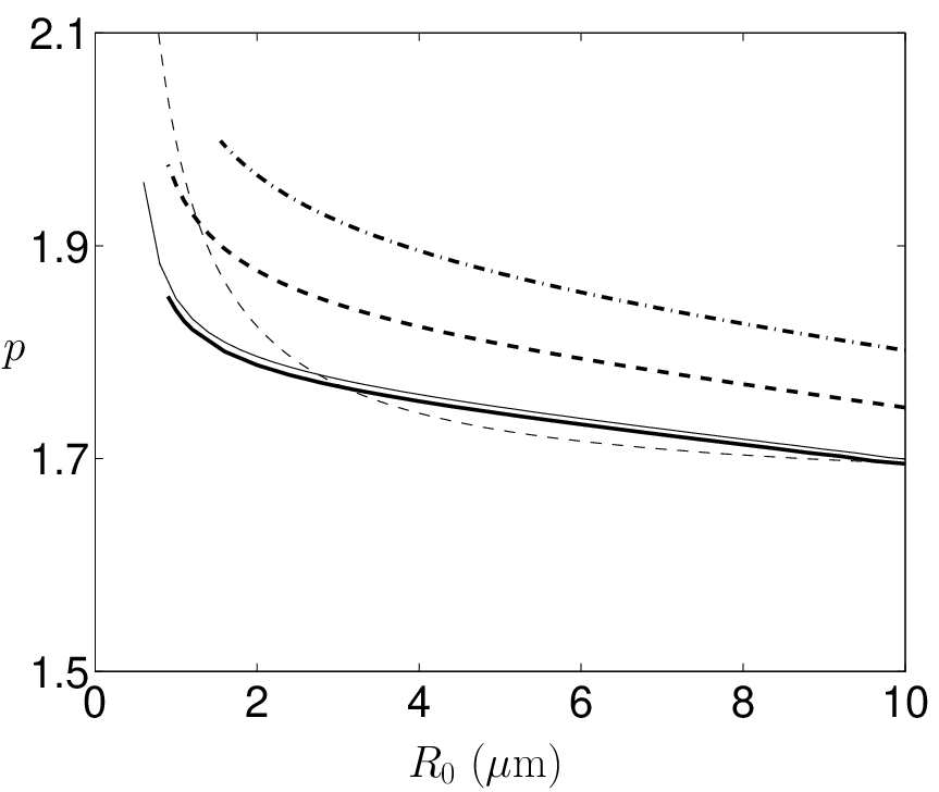
Figure 2 represents the variations of for a bubble of ambient radius 1 m (fig. 2.a) and 3 m (fig. 2.b) in water. The thick solid lines are the exact value obtained numerically, and the thin solid lines represent . The agreement is seen to be excellent, although a noticeable difference can be seen for 1 m, which originates from the over-simplification done when accounting for surface tension by the simple term in Eq. (16). Also shown is the approximation (dash-dotted line), which does not take surface tension into account. This clearly introduces an noticeable error on , reasonably corrected by Eq. (32). Finally, the approximation proposed in Ref. [1] is displayed (dotted line).

Finally, the approximation of can then easily be obtained by plugging an approximation of into Eq. (24). This was done in Ref. 35 using , and an excellent agreement was found. The gain brought by using instead of in (24) remains unimportant, and for brevity, we do not present the comparison between the analytical and numerical expressions of here.
III.2 Bubble volume
Approximations of the bubble volume could readily be obtained from the approximations (21), (22) of the bubble radius. However, such expressions do not yield analytical expressions of the integral (14) in closed form, and further approximations are therefore required. First, we consider frequencies low enough to have , so that the term can be safely neglected in equations (21)-(22).
III.2.1 Approximate expression on
Numerical simulations demonstrate that is almost linear between 0 and (Fig. 1.a), which suggests that Eq. (21) is almost a perfect square in this interval. We then develop the term in (21) near up to second order, and write the result as
| (34) |
For to be linear in , the constant term in the bracket must be negligible, so that can be simplified as
| (35) |
The expression of the bubble volume on therefore reads
III.2.2 Approximate expression on
Using equations (23) and (24), it can be easily checked that, setting , the expression (22) of can be recast as:
| (38) |
where
| (39) | |||||
The bubble volume on becomes therefore
| (40) |
which unfortunately does not yield an explicit integration of (14). Further progress can be done by noting that, from Eq. (24), and are of the same order of magnitude, and that from (39), near . Equation (40) can therefore be approximated by
| (41) |
Thus, to the same order of approximation, can be replaced by any equivalent expression up to order 4 in , and the choice must be directed by the ability of to be integrable in closed form. We therefore choose to set and in Eq. (39) to finally obtain:
| (42) | |||||
which can now yield an explicit expression for integral (14).
It can further be noted that neglecting the term in the square bracket, and setting , is found to be zero for
| (43) |
which constitutes a simple approximation of the collapse-time. The comparison between this expression and the exact instant of minimum radius is visible in Fig. 2 (dashed lines). Here again, an excellent agreement is found, but deteriorates toward small bubble radii.
IV Bjerknes force
IV.1 Analytical expression
With the expressions of the bubble volume (36) and (42) at hand, the integral (14) can be calculated in analytical form, keeping the contribution of the integrand only in the intervals and , since can be neglected in the other regions (see Fig. 1.b). The integral is thus the sum of the two contributions:
| (44) |
where
Using the approximate expressions (36) and (42) of the bubble volume, integration yields
| (45) | |||||
with
The contribution reads
| (46) | |||||
where
and
The value of from (44)-(46) is displayed in figure 3 (thick lines) for m (Fig. 3a), 3 m (Fig. 3b), and 6 m (Fig. 3c), in the case of a standing wave (), for drivings ranging from the Blake threshold to . In order to get a clear picture, is drawn in logarithmic scale, the solid part of the curves representing a positive sign and the dashed part a negative sign. The thin lines are the results obtained by solving (4) and calculating (14) numerically, for kHz. It is seen that an excellent agreement is obtained, except for m (Fig 3a). Particularly, the point of inversion of the Bjerknes force is shifted toward large drivings. This feature originates from the errors induced on the values of , (see Fig. 2) and for small ambient radii, by replacing the surface tension in the RP equation by in (16). It should be noticed that even the small errors visible on the curves of Fig. 2.a yields large differences on the estimation of . This could be expected since the phase between and crucially influences the value of integral .

IV.2 Bjerknes force inversion threshold in standing waves
We consider the case of a standing wave , and look for an approximate locus in the parameter space where the Bjerknes force changes sign. Summing equations (45) and (46), it is seen that integral (14) is zero for
| (47) |
where
and the coefficients depend on
- •
, which is just ,
- •
, which from (37) depends on and ,
- •
, which from (43) depends on , , and ,
- •
, which from (32), only depends on and , for .
Furthermore, looking at Eq. (24), for , can be written as
| (48) |
and from Eqs. (25)-(27) and (30)-(33), still under the assumption , the terms , in the above equation depend on only through . We conclude that, provided that , equation (47) becomes frequency independent, and can in fact be written in implicit form as
| (49) |
This equation can easily be solved for , in order to find the approximate, frequency-independent threshold for inversion of the Bjerknes force. The solution is presented in the inset of Fig. (4). Below the curve, , so that the Bjerknes force attracts the bubble toward pressure antinodes, while it becomes repulsive above.
From , the inversion threshold can also be plotted in the plane in the case of water at ambient pressure ( N.m-1, Pa). The result is displayed in Fig. 4 (thick solid line) and compared to the exact inversion thresholds calculated from numerical simulation for three driving frequencies 20 kHz (dash-dotted line), 40 kHz (dashed line), and 80 kHz (thin solid line). The labels on the two latter curves represent the value of . It is seen that the above procedure yields a good estimation of the inversion threshold, up to , above which it starts to diverge from the exact value. The reasons for this disagreement comes from the neglected term in all expressions, and also from the fact that for increasing frequency, the bubble rebounds become more important, so that the bubble dynamics for also contributes to expression (14). Besides, a cascade of period-doubling bifurcations and chaos [36, 37, 19] appear in some cases (and are responsible for the noisy oscillations on the 80 kHz curve), so that the correct averaging of the Bjerknes force in such cases should be carried out over more than a single acoustic period. We did not pursue further this issue, since analytical predictions for these bifurcations are out of the scope of the present paper.

Marginally, it can be seen that the inversion threshold in the plane is almost linear, so that the following linear fit (represented by a dashed line in the inset of Fig. 4) can be proposed for practical applications:
| (50) |
These results suggest that the inversion threshold is independent of frequency, and of the properties of the gas and liquid other than surface tension, as long as . This astonishing result originates from the fact that the Bjerknes force mainly depends on the expansion phase of the bubble, which, within the approximations leading to Eq. (16), is merely governed by the driving pressure amplitude and surface tension. The reasonably good agreement found in Figs. 2-4 partially supports this analysis.
In order to further investigate this issue, we first recalculated the three inversion thresholds of Fig. 4 ( 20, 40, 80 kHz), replacing the thermal model of Ref. 32 by an isothermal behavior for the bubble interior. Figure 5 displays the results obtained (thick solid lines) and recalls the thresholds calculated in Fig. 4 (thin solid lines). It can be seen that the thresholds slightly diverge for increasing , but remain almost indistinguishable for We also repeated the calculations with the thermal model of Ref. 32, but for argon bubbles (not shown), and found a negligible deviation from the air curves. We therefore conclude that the detailed bubble interior has a very weak influence on the expansion phase, at least for low enough values of , so that Eq. (50) indeed constitutes a gas-independent law, within its range of validity.

Another issue is the sensitivity of the results to the liquid viscosity. The latter has been neglected in the analytical approach, when approximating the RP equation (8) by Eq. (16). The good agreement found in Fig. 4 between analytical and numerical results, calculated for water at ambient temperature ( Pa.s), suggests that for such low values, viscosity indeed plays a minor role during the bubble expansion. One should however check whether it is still the case for larger viscosities. We therefore repeated the calculation of the inversion threshold for viscosities 10 and 20 times larger than the one of water (Fig. 6, thick dashed line and thick dash-dotted line). It is clearly seen that the threshold increases noticeably with viscosity. Conversely, we also checked that the result was unaffected by decreasing the viscosity below the water’s one, by computing the threshold for (thick solid line). This indicates that viscous friction plays a non-negligible role in the bubble expansion for viscosities above some critical value. As already mentioned in Ref. 1, increasing viscosity decreases , and we also checked that it decreases too, so that, strictly speaking, the Bjerknes force and its inversion threshold are viscosity-dependent. Following our results, this influence is negligible for viscosities near or lower than the water’s one, but for slightly larger values, the viscous term should be kept in the RP equation.
V Discussion
Important conclusions can be drawn from these results. Figure 4 shows that the inversion thresholds for all frequencies (thin lines) asymptotically merge with the Blake threshold (thick dashed line) for small bubble radii, and in reasonable agreement with the analytical approximation (thick solid line). Thus, as the driving pressure reaches, say 1.8 bar, the range of ambient radii of inertial bubbles attracted toward the antinode is suddenly reduced, with an upper limit lower than 2 m. This explains why a well-defined bubble-free region can be observed around the pressure antinode for high amplitude standing waves [21]. The range of attracted bubbles is however not void, which suggests that the zone around the antinode could still be filled with inertial bubbles, of ambient radii very close to the Blake threshold, but too small to be visible. As noticed in Ref. [18], in a high amplitude standing wave, the Bjerknes force acts as a sorter of inertial bubbles, leaving the smallest ones approaching or even reaching the pressure antinodes. The advantage of the present analysis is that it yields, through Eq. (49), or its simpler form (50), an explicit classification of the bubble sizes as a function of the local acoustic pressure, parametrized by the ratio .
As the increasingly small bubbles approach the pressure antinode, they may coalesce or quickly grow by rectified diffusion [35]. Increasing their size, they may again enter the repulsion zone in the plane and move back again. This picture is still complicated by the potential appearance of surface instabilities. Thus, the apparently void region observed around large pressure antinodes may be in fact the locus of the complex evolution of very small bubbles, of sizes close to the Blake threshold.
Finally, it is seen from the inset of Fig. 4 that decreasing lowers the driving at which the pressure antinode becomes repulsive. The dimensionless parameter can be varied experimentally by modifying the surface tension (for example adding ionic salts or surfactants), or by changing the static pressure . The present results suggest that, for identical bubble ambient radii, the Bjerknes force would become repulsive for lower drivings, when either decreasing or increasing . This should have an observable effect on the size of the bubble-free region around the pressure antinode. However, it should be noted that surface tension also plays a crucial role for bubbles surface instabilities [38, 39, 10], and also for rectified diffusion [35], through the same dimensionless parameter . Thus, changing may also directly influence these two processes, with probable consequences on the bubble cloud behavior. The present result just demonstrates that surface tension can influence the shape of the bubble cloud through its direct effect on the bubble dynamics, and on the primary Bjerknes force.
Figure 6 also indicates that the size of the bubble-free region around the pressure antinode would decrease noticeably when increasing viscosity slightly above the one of water. As mentioned in Ref. 1, this may be easily achieved experimentally by adding glycerin in water. Here again, such a macroscopic effect is mediated by the sensitivity of the bubble dynamics to the physical properties. To account analytically for this dependence on viscosity, the viscous term should be kept in the Rayleigh equation, which renders the approximation scheme more involved. A generalization of our analytical results to this case may be addressed in a future study.
Finally, it is highly probable that the same effect of surface tension could be observed on the secondary Bjerknes force, as suggested by numerical simulations [40]. The extension of the present analytical method to the latter effect is difficult, first because the expression of the secondary Bjerknes force also involves the bubbles velocities, which are much more sensitive to approximations than the bubble radius itself, and secondly because the dynamics equation of the two bubbles must be coupled by a radiation term.
References
- [1] S. Hilgenfeldt, M. P. Brenner, S. Grossman, and D. Lohse, J. Fluid Mech. 365, 171 (1998).
- [2] F. G. Blake, Harvard Univ. Acoust. Res. Lab. Tech. Mem. (1949a).
- [3] E. A. Neppiras, Phys. Rep. 61, 159 (1980).
- [4] I. Akhatov, N. Gumerov, C. D. Ohl, U. Parlitz, and W. Lauterborn, Phys. Rev. Lett. 78, 227 (1997a).
- [5] K. S. Suslick, W. B. McNamara, and Y. Didenko, in Sonochemistry and Sonoluminescence, edited by L. A. Crum, T. J. Mason, J. L. Reisse, and K. S. Suslick (Kluwer Academic, Dordrecht, 1999), pp. 191–204, proceedings of the NATO Advanced Study Institute on Sonoluminescence and Sonoluminescence, Leavenworth, Washington, USA, 18-29 August 1997.
- [6] W. Lauterborn, T. Kurz, R. Mettin, and C. D. Ohl, Adv. Chem. Physics 110, 295 (1999).
- [7] D. Krefting, R. Mettin, and W. Lauterborn, Ultrasonics Sonochemistry 11, 119 (2004).
- [8] D. F. Gaitan, L. A. Crum, C. C. Church, and R. A. Roy, J. Acoust. Soc. Am. 91, 3166 (1992).
- [9] S. J. Putterman and K. R. Weninger, Ann. Rev. of Fluid Mech. 32, 445 (2000).
- [10] M. P. Brenner, S. Hilgenfeldt, and D. Lohse, Rev. Mod. Phys. 74, 425 (2002).
- [11] J. Magnaudet, in ASME Fluids Engineering Division Summer Meeting (1997).
- [12] V. F. K. Bjerknes, Fields of Force (Columbia University Press, New York, 1906).
- [13] F. G. Blake, J. Acoust. Soc. Am. 21, 551 (1949b).
- [14] D. E. Goldman and G. R. Ringo, J. Acoust. Soc. Am. 21, 270 (1949).
- [15] L. A. Crum and A. I. Eller, J. Acoust. Soc. Am. 48, 181 (1970).
- [16] T. G. Leighton, A. J. Walton, and M. J. W. Pickworth, Eur. J. Phys. 11, 47 (1990).
- [17] B. P. Barber, R. A. Hiller, R. Löfstedt, S. J. Putterman, and K. R. Weninger, Phys. Rep. 281, 65 (1997).
- [18] I. Akhatov, R. Mettin, C. D. Ohl, U. Parlitz, and W. Lauterborn, Phys. Rev. E 55, 3747 (1997b).
- [19] W. Lauterborn and R. Mettin, in Sonochemistry and Sonoluminescence, edited by L. A. Crum, T. J. Mason, J. L. Reisse, and K. S. Suslick (Kluwer Academic, Dordrecht, 1999), pp. 63–72, proceedings of the NATO Advanced Study Institute on Sonoluminescence and Sonoluminescence, Leavenworth, Washington, USA, 18-29 August 1997.
- [20] R. Mettin, S. Luther, C. D. Ohl, and W. Lauterborn, Ultrason. Sonochem. 6, 25 (1999).
- [21] U. Parlitz, R. Mettin, S. Luther, I. Akhatov, M. Voss, and W. Lauterborn, Phil. Trans. R. Soc. Lond. A 357, 313 (1999).
- [22] P. Koch, D. Krefting, R. Mettin, and W. Lauterborn, in Proceedings of the IEEE International Ultrasonics Symposium, Honolulu, USA (Honolulu, USA, 2003), pp. 1475–1478.
- [23] R. Mettin, in Oscillations, Waves and Interactions, edited by T. Kurz, U. Parlitz, and U. Kaatze (Universitätsverlag Göttingen, 2007), pp. 171–198.
- [24] R. Löfstedt, B. P. Barber, and S. J. Putterman, Phys. Fluids A5, 2911 (1993).
- [25] L. Rayleigh, Phyl. Mag. 34, 94 (1917).
- [26] E. A. Neppiras and B. E. Noltingk, Proc. Phys. Soc B63, 1032 (1951).
- [27] H. Lin, B. D. Storey, and A. J. Szeri, J. Fluid Mech. 452, 145 (2002).
- [28] A. Prosperetti, J. Fluid. Mech. 222, 587 (1991).
- [29] A. Prosperetti and Y. Hao, Phil. Trans. R. Soc. Lond. A 357, 203 (1999).
- [30] A. Prosperetti, in Sonochemistry and Sonoluminescence, edited by L. A. Crum, T. J. Mason, J. L. Reisse, and K. S. Suslick (Kluwer Academic, Dordrecht, 1999), pp. 39–62, proceedings of the NATO Advanced Study Institute on Sonoluminescence and Sonoluminescence, Leavenworth, Washington, USA, 18-29 August 1997.
- [31] B. D. Storey and A. Szeri, Proc. R. Soc. London, Ser. A 457, 1685 (2001).
- [32] R. Toegel, B. Gompf, R. Pecha, and D. Lohse, Phys. Rev. Lett. 85, 3165 (2000).
- [33] J. B. Keller and I. I. Kolodner, J. Appl. Phys. 27, 1152 (1956).
- [34] A. Prosperetti and A. Lezzi, J. Fluid Mech. 168, 457 (1986).
- [35] O. Louisnard and F. Gomez, Phys. Rev. E 67, 036610-1 (2003).
- [36] W. Lauterborn and E. Cramer, Phys. Rev. Lett. 47, 1445 (1981).
- [37] U. Parlitz, V. English, C. Scheffczyk, and W. Lauterborn, J. Acoust. Soc. Am. 88, 1061 (1990).
- [38] M. S. Plesset, J. Appl. Phys. 25, 96 (1954).
- [39] Y. Hao and A. Prosperetti, Phys. Fluids 11, 1309 (1999).
- [40] R. Mettin, I. Akhatov, U. Parlitz, C. D. Ohl, and W. Lauterborn, Phys. Rev. E 56, 2924 (1997).