跳到论文正文
W Papers独立论文阅读器 arXiv:1302.5828 论文正文 计算阅读时间 · 0%
引用这篇论文根据当前论文元数据生成,正式投稿前建议核对。


License: arXiv.org perpetual non-exclusive license
arXiv:1302.5828v3 [math.AP] 17 Dec 2013

A Hamilton-Jacobi equation for the continuum limit of non-dominated sortingThanks: The research described in this paper was partially supported by ARO grant W911NF-09-1-0310 and NSF grants CCF-1217880 and DMS-0914567.

Jeff Calder ††thanks: Department of Mathematics, University of Michigan. ({jcalder,esedoglu}@umich.edu)    Selim Esedoḡlu††footnotemark:    Alfred O. Hero ††thanks: Department of Electrical Engineering and Computer Science, University of Michigan. (hero@eecs.umich.edu)
Abstract

We show that non-dominated sorting of a sequence X1,…,XnX_{1},\dots,X_{n} of i.i.d. random variables in ℝd\mathbb{R}^{d} has a continuum limit that corresponds to solving a Hamilton-Jacobi equation involving the probability density function ff of XiX_{i}. Non-dominated sorting is a fundamental problem in multi-objective optimization, and is equivalent to finding the canonical antichain partition and to problems involving the longest chain among Euclidean points. As an application of this result, we show that non-dominated sorting is asymptotically stable under bounded random perturbations in X1,…,XnX_{1},\dots,X_{n}. We give a numerical scheme for computing the viscosity solution of this Hamilton-Jacobi equation and present some numerical simulations for various density functions.

1 Introduction

Let X1,…,XnX_{1},\dots,X_{n} be i.i.d. random variables on ℝd\mathbb{R}^{d} with density function f∈L1​(ℝd)f\in L^{1}(\mathbb{R}^{d}). The points form a partially ordered set 𝒳n={X1,…,Xn}{\mathcal{X}}_{n}=\{X_{1},\dots,X_{n}\} under the partial order

x≦y⇔xi≤yi​ for ​i=1,…,d.x\leqq y\iff x_{i}\leq y_{i}\ \text{ for }\ i=1,\dots,d. (1.1)

Let ℓ⁡(n)\ell(n) denote the length of a longest chain11 1 A chain is a totally ordered subset of 𝒳n{\mathcal{X}}_{n}. in 𝒳n{\mathcal{X}}_{n}, and for x∈ℝdx\in\mathbb{R}^{d} let un​(x)u_{n}(x) denote the length of a longest chain in 𝒳n{\mathcal{X}}_{n} consisting of points less than xx. We are interested in the asymptotic properties of unu_{n} as n→∞n\to\infty.

When ff is a smooth density on [0,1]d[0,1]^{d}, hence ℓ⁡(n)=un​(1,…,1)\ell(n)=u_{n}(1,\dots,1), the problem of studying the asymptotics of ℓ⁡(n)\ell(n) has a long history. It begins with Ulam’s famous problem [44] of finding the length of a longest increasing subsequence of a random permutation. Hammersley [24] made some of the first breakthroughs in understanding Ulam’s problem. He observed that the distribution of the length of a longest increasing subsequence among nn numbers chosen uniformly at random is the same as the distribution of ℓ⁡(n)\ell(n) for uniformly distributed points on [0,1]2[0,1]^{2}. Using subadditive ergodic theory, Hammersley showed that n−12​ℓ​(n)n^{-\frac{1}{2}}\ell(n) converges almost surely to a constant cc as n→∞n\to\infty, and he conjectured that c=2c=2. In subsequent papers, Vershik and Kerov [45] and Logan and Shepp [31] showed that c≤2c\leq 2 and c≥2c\geq 2, respectively. Hammersley’s results were generalized by Bollobás and Winkler [6] to uniformly distributed points on [0,1]d[0,1]^{d}; they showed that there exist positive constants cdc_{d} such that n−1d​ℓ​(n)→cdn^{-\frac{1}{d}}\ell(n)\to c_{d} almost surely as n→∞n\to\infty, and cd\nnearrowec_{d}\nnearrow e as d→∞d\to\infty. The only known values of cdc_{d} are c1=1c_{1}=1 and c2=2c_{2}=2. Deuschel and Zeitouni [15] generalized Hammersley’s results in another direction. For X1,…,XnX_{1},\dots,X_{n} i.i.d. on [0,1]2[0,1]^{2} with C1C^{1} density function f:[0,1]2→ℝf:[0,1]^{2}\to\mathbb{R}, bounded away from zero, they showed that n−12​ℓ​(n)→2​J¯n^{-\frac{1}{2}}\ell(n)\to 2{\overline{J}} in probability, where J¯{\overline{J}} is the supremum of the energy

J⁡(φ)=∫01φ′​(x)​f​(x,φ⁡(x))​𝑑x,J(\varphi)=\int_{0}^{1}\sqrt{\varphi^{\prime}(x)f(x,\varphi(x))}\,dx,

over all φ:[0,1]→[0,1]\varphi:[0,1]\to[0,1] nondecreasing and right continuous.

There is another motivation for studying the asymptotics of unu_{n} that arises in multi-objective optimization problems. Such problems are of immense importance in many fields of science and engineering, including control theory and path planning [34, 30, 33], gene selection and ranking [41, 27, 26, 28, 17, 18, 19], data clustering [25], database systems [29, 37] and image processing and computer vision [35, 10]. In a discrete multi-objective optimization problem, one has several objective functions gi:S→[0,∞)g_{i}:S\to[0,\infty), where i=1,…,di=1,\dots,d and S={x1,…,xn}S=\{x^{1},\dots,x^{n}\} is a finite set, and is tasked with finding an element x∈Sx\in S that minimizes all of the functions simultaneously. This is generally an impossible task, and instead, a family of solutions are obtained based on the notion of Pareto-optimality. A feasible solution x∈Sx\in S is called Pareto-optimal if for every y∈Sy\in S, we have gi​(y)>gi​(x)g_{i}(y)>g_{i}(x) for some ii, or gi​(y)=gi​(x)g_{i}(y)=g_{i}(x) for all ii; in other words, no other feasible solution is better in every objective. The collection of Pareto-optimal elements is denoted ℱ1{\mathcal{F}}_{1} and called the first Pareto front. It is the most natural notion of solution for a discrete multi-objective optimization problem. If we set Xi=(g1​(xi),…,gd​(xi))∈ℝdX_{i}=(g_{1}(x^{i}),\dots,g_{d}(x^{i}))\in\mathbb{R}^{d} for i=1,…,ni=1,\dots,n, then assuming all XiX_{i} are distinct, it is not hard to see that

xi∈ℱ1⇔un​(Xi)=1.x^{i}\in{\mathcal{F}}_{1}\iff u_{n}(X_{i})=1.

The second Pareto front, ℱ2{\mathcal{F}}_{2}, consists of the Pareto-optimal elements of S∖ℱ1S\setminus{\mathcal{F}}_{1}, and in general

ℱk=Pareto​optimal​elements​of​S∖⋃j<kℱj.{\mathcal{F}}_{k}={\rm Pareto\ optimal\ elements\ of\ }S\setminus\bigcup_{j<k}{\mathcal{F}}_{j}.

The Pareto front that a particular feasible solution lies on is useful for ranking feasible solutions. As before, when the XiX_{i} are all distinct we have

xi∈ℱk⇔un​(Xi)=k.x^{i}\in{\mathcal{F}}_{k}\iff u_{n}(X_{i})=k.

This observation is essential. It says that studying the asymptotic shapes of the Pareto fronts ℱ1,ℱ2,…{\mathcal{F}}_{1},{\mathcal{F}}_{2},\dots is equivalent to studying the longest chain function unu_{n}. Figure 1(a) shows the Pareto fronts for n=50n=50 points uniformly distributed on [0,1]2[0,1]^{2}, and Figure 1(b) shows the Pareto fronts for n=106n=10^{6} points. The points XiX_{i} that are on the same Pareto front are connected by a continuous staircase curve that represents the jump set of unu_{n}.

(a) n=50n=50 points
(b) n=106n=10^{6} points
Figure 1: Examples of Pareto fronts for X1,…​XnX_{1},\dots X_{n} chosen from the uniform distribution on [0,1]2[0,1]^{2}. In (b), 2929 equally spaced fronts are depicted.

In the multi-objective optimization literature, the process of computing the Pareto fronts for a collection of points is called non-dominated sorting [13]. In the combinatorics literature, the partition S=ℱ1∪ℱ2∪⋯S={\mathcal{F}}_{1}\cup{\mathcal{F}}_{2}\cup\cdots is called the canonical antichain partition [16]. Although we have described non-dominated sorting in the context of a discrete optimization problem, it is a fundamental tool in continuous optimization as well. Many state of the art algorithms for continuous optimization involve a large number of discrete subproblems, each of which requires non-dominated sorting. The most common examples are the so-called genetic and evolutionary algorithms for continuous multi-objective optimization [13, 20, 21, 12, 42]. The applications of non-dominated sorting are not restricted to optimization; indeed, there are further striking applications in combinatorics [16, 32], molecular biology [38, 1], graph theory [32], Young Tableaux [46, 16] and even in physical layout problems in the design of integrated circuits [1].

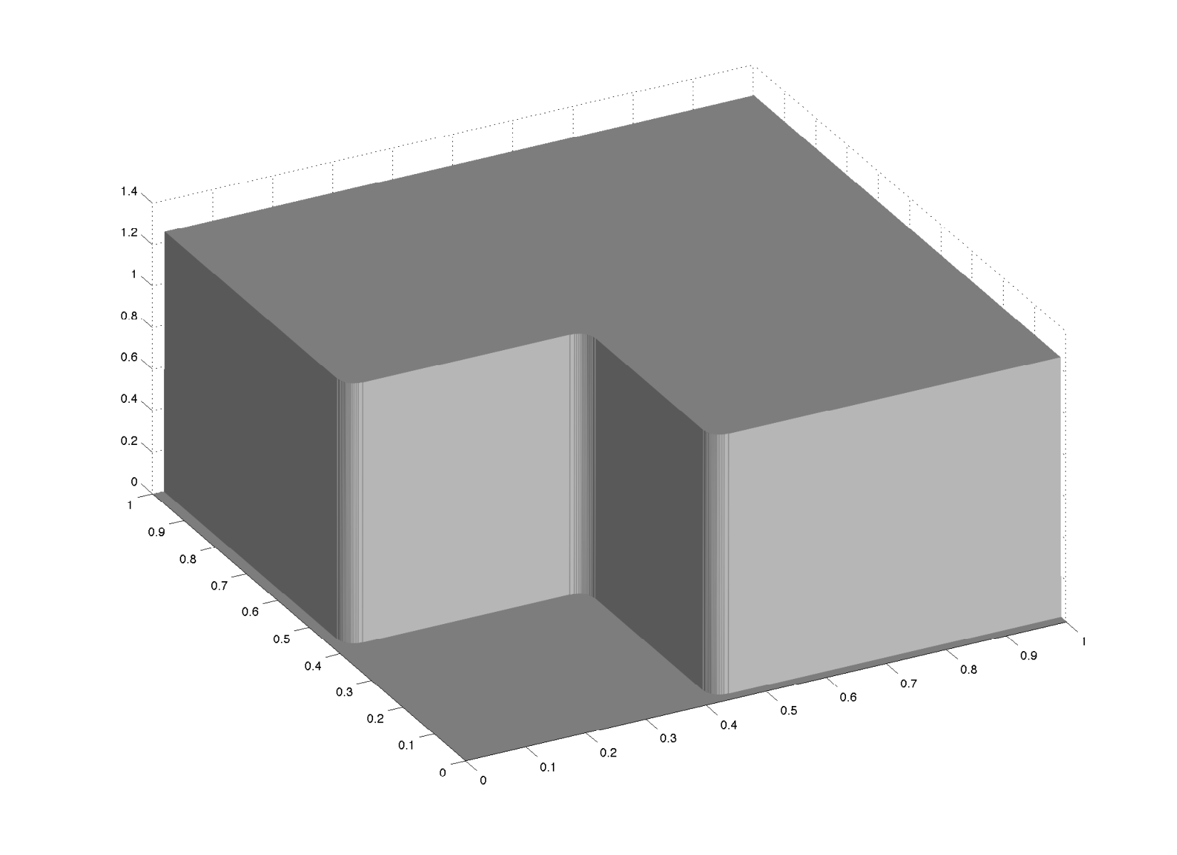
The goal of this paper is to study the asymptotics of unu_{n}, and hence the asymptotics of non-dominated sorting. Our main result, Theorem 1, states that n−1d​unn^{-\frac{1}{d}}u_{n} converges almost surely to a continuous function UU, which is the viscosity solution of a Hamilton-Jacobi equation. Our proof is based on linking the asymptotics of unu_{n} to a variational problem, which is a generalization of the variational problem discovered by Deuschel and Zeitouni [15] to higher dimensions. The Hamilton-Jacobi equation satisfied by UU is the Hamilton-Jacobi-Bellman equation [3] for the corresponding variational problem. We describe our main result in Section 1.1, and postpone the proofs to Sections 2 and 3. In Section 4, we give a numerical scheme for computing UU, and show simulation results comparing the level sets of UU to Pareto fronts for various density functions.

1.1 Main result

For x,y∈ℝdx,y\in\mathbb{R}^{d}, we write x≤yx\leq y if x≦yx\leqq y and x≠yx\neq y. When xi<yix_{i}<y_{i} for i=1,…,di=1,\dots,d, we write x<yx<y, and we set ℝ+d={x∈ℝd:x>0}\mathbb{R}^{d}_{+}=\{x\in\mathbb{R}^{d}\,:\,x>0\}. We will always assume d≥2d\geq 2. For s,t∈ℝs,t\in\mathbb{R}, s≤ts\leq t and s<ts<t will retain their usual definitions. Let Ω⊂ℝd\Omega\subset\mathbb{R}^{d} and let f:ℝd→[0,∞)f:\mathbb{R}^{d}\to[0,\infty). We place the following assumptions on ff and Ω\Omega.

  • (H1)

    There exists a continuous nondecreasing function m:[0,∞)→[0,∞)m:[0,\infty)\to[0,\infty) satisfying m⁡(0)=0m(0)=0 such that

    |f⁡(x)−f⁡(y)|≤m⁡(|x−y|),|f(x)-f(y)|\leq m(|x-y|),

    for x,y∈Ωx,y\in\Omega, and f⁡(x)=0f(x)=0 for x∉Ωx\not\in\Omega,

  • (H2)

    Ω⊂ℝ+d\Omega\subset\mathbb{R}^{d}_{+} is open and bounded with Lipschitz boundary.

Set

𝒜={γ∈C1​([0,1],ℝd):γ′​(t)≥0​ for all ​t∈[0,1]}.{\mathcal{A}}=\left\{\gamma\in C^{1}([0,1];\mathbb{R}^{d})\,:\,{\gamma\>}^{\prime}(t)\geq 0\ \text{ for all }\ t\in[0,1]\right\}. (1.2)

Recall that γ′​(t)≥0{\gamma\>}^{\prime}(t)\geq 0 means that γi′​(t)≥0\gamma_{i}\hskip-0.7113pt^{\prime}(t)\geq 0 for i=1,…,di=1,\dots,d and γ′​(t)≠0{\gamma\>}^{\prime}(t)\neq 0. Define J:𝒜→[0,∞)J:{\mathcal{A}}\to[0,\infty) by

J(γ)=∫01f(γ(t))1d(γ1′(t)⋯γd′(t))1ddt,J(\gamma)=\int_{0}^{1}f(\gamma(t))^{\frac{1}{d}}(\gamma_{1}\hskip-2.13394pt^{\prime}(t)\cdots\gamma_{d}\hskip-2.13394pt^{\prime}(t))^{\frac{1}{d}}\,dt, (1.3)

and U:ℝd→ℝU:\mathbb{R}^{d}\to\mathbb{R} by

U(x)=supγ∈𝒜:γ⁡(1)≦xJ(γ).U(x)=\sup_{\gamma\in{\mathcal{A}}\,:\,\gamma(1)\leqq x}J(\gamma). (1.4)

We make the following definition.

Definition 1.

Given a domain 𝒪⊂ℝd{\mathcal{O}}\subset\mathbb{R}^{d}, we say that a function u:𝒪→ℝu:{\mathcal{O}}\to\mathbb{R} is Pareto-monotone if x≦y⟹u⁡(x)≤u⁡(y)x\leqq y\implies u(x)\leq u(y) for all x,y∈𝒪x,y\in{\mathcal{O}}.

In Section 2, we show that UU is a Pareto-monotone viscosity solution of the Hamilton-Jacobi partial differential equation (PDE)

{Ux1⋯Uxd=1ddf on ℝ+dU=0 on ∂ℝ+d.\begin{cases}U_{x_{1}}\cdots U_{x_{d}}=\frac{1}{d^{d}}f&\ \ \text{ on }\ \ \mathbb{R}^{d}_{+}\\ U=0&\ \ \text{ on }\ \ \partial\mathbb{R}^{d}_{+}.\end{cases} (1.5)

The PDE (1.5) should be interpreted as the Hamilton-Jacobi-Bellman equation for the value function UU. We note that ff need only be Borel-measurable, bounded and have compact support in ℝ+d\mathbb{R}^{d}_{+} for UU to be a viscosity solution of (1.5). The stronger assumptions (H1) and (H2) are needed to prove that UU is the unique Pareto-monotone viscosity solution of (1.5) (see Theorem 5) under an appropriate boundary condition at infinity. Our main result is

Theorem 1.

Let ff satisfy (H1), let Ω\Omega satisfy (H2), and let X1,…,XnX_{1},\dots,X_{n} be i.i.d. with density ff. Then there exists a positive constant cdc_{d} such that

n−1d​un⟶cd​U in ​L∞​(ℝd)​ almost surely.n^{-\frac{1}{d}}u_{n}\longrightarrow c_{d}U\ \ \text{ in }\ L^{\infty}(\mathbb{R}^{d})\ \text{ almost surely.}

The constants cdc_{d} are the same as those given by Bollobás and Winkler [6]. In particular, c1=1c_{1}=1, c2=2c_{2}=2 and cd\nnearrowec_{d}\nnearrow e as d→∞d\to\infty. When ff is a product density, i.e., f(x)=f1(x1)⋯fd(xd)f(x)=f_{1}(x_{1})\cdots f_{d}(x_{d}), the value function UU is given by

U(x)=(∫0≦y≦xf(y)dy)1d=(∫0xif1(t)dt)1d⋯(∫0xdfd(t)dt)1d.U(x)=\left(\int_{0\leqq y\leqq x}f(y)\,dy\right)^{\frac{1}{d}}=\left(\int_{0}^{x_{i}}f_{1}(t)\,dt\right)^{\frac{1}{d}}\cdots\left(\int_{0}^{x_{d}}f_{d}(t)\,dt\right)^{\frac{1}{d}}. (1.6)

For the case f=1f=1 and d=2d=2, Aldous and Diaconis [2, p. 204] provided a non-rigorous derivation of (1.5) by viewing the problem as an interacting particle process. They used this to motivate their proof that c=2c=2 in Ulam’s problem, but make no rigorous statements about the relationship between (1.5) and the longest chain problem. A similar, though tangentially related, PDE also appears in growth models in multiple dimensions that are defined through the height of a random partial order [39, p. 209].

Theorem 1 provides a new tool with which to study the asymptotics of non-dominated sorting and the longest chain problem. As an example of the applicability of this result, we show in Theorem 10 that non-dominated sorting is asymptotically stable under bounded random perturbations. Evidently, Theorem 1 reduces the problem of non-dominated sorting to solving a Hamilton-Jacobi equation. From an algorithmic perspective, this may be useful in designing fast approximate algorithms for non-dominated sorting, or finding lengths of longest chains. We study some of these applications in a subsequent paper [7].

1.2 Motivation

As motivation, let us give an informal derivation of the Hamilton-Jacobi PDE (1.5). Suppose f:ℝd→ℝf:\mathbb{R}^{d}\to\mathbb{R} is continuous and n−1d​un→U∈C1​(ℝd)n^{-\frac{1}{d}}u_{n}\to U\in C^{1}(\mathbb{R}^{d}) uniformly. Fix nn large enough so that n−1d​un≈Un^{-\frac{1}{d}}u_{n}\approx U. Then the kthk^{\rm th} Pareto front should be well approximated by the level set {y:U⁡(y)=n−1d​k}\{y\,:\,U(y)=n^{-\frac{1}{d}}k\}. It is not hard to see that UU should be Pareto-monotone (recall Definition 1), and hence it is reasonable to assume that Uxi>0U_{x_{i}}>0 for all ii. Fix x,v∈ℝdx,v\in\mathbb{R}^{d} with ⟨D​U​(x),v⟩>0\langle DU(x),v\rangle>0, where D​U​(x)DU(x) denotes the gradient of UU at xx, and consider the quantity n1d​(U⁡(x+v)−U⁡(x))n^{\frac{1}{d}}(U(x+v)-U(x)). This is approximately the number of Pareto fronts passing between xx and x+vx+v. When counting these fronts, we may restrict ourselves to the region

A={y:U⁡(y)≥U⁡(x)​ and ​y≦x+v}.A=\{y\,:\,U(y)\geq U(x)\ \text{ and }\ y\leqq x+v\}.

This is because any samples in {y:U⁡(y)<U⁡(x)}\{y\,:\,U(y)<U(x)\} will be on a previous Pareto front and only samples that are less than x+vx+v can influence the Pareto rank of x+vx+v. See Figure 2 for a depiction of this region and some quantities from the derivation.

Figure 2: Some quantities from the informal derivation of the Hamilton-Jacobi PDE (1.5).

Since Uxi​(x)>0U_{x_{i}}(x)>0 for all ii, and UU is C1C^{1}, AA is well approximated by a simplex for small |v||v|, and furthermore, the samples within AA are approximately uniformly distributed. Let mm denote the number of samples falling in AA. By scaling the simplex into a standard simplex, without disrupting the Pareto ordering within AA, it is reasonable to conjecture that the number of Pareto fronts within AA (or the length of a longest chain in AA) is approximately c​m1dcm^{\frac{1}{d}} for some constant cc, independent of xx. For simplicity we take c=1c=1.

By the law of large numbers, we have m≈n​∫Af⁡(y)​𝑑ym\approx n\int_{A}f(y)\,dy. Hence when |v|>0|v|>0 is small we have

n1d​(U⁡(x+v)−U⁡(x))≈(n​∫Af⁡(y)​𝑑y)1d≈n1d​|A|1d​f​(x)1d,n^{\frac{1}{d}}(U(x+v)-U(x))\approx\left(n\int_{A}f(y)\,dy\right)^{\frac{1}{d}}\approx n^{\frac{1}{d}}|A|^{\frac{1}{d}}f(x)^{\frac{1}{d}}, (1.7)

where |A||A| denotes the Lebesgue measure of AA. Let ℓ1,…,ℓd\ell_{1},\dots,\ell_{d} denote the side lengths of the simplex AA. Then |A|≈cℓ1⋯ℓd|A|\approx c\,\ell_{1}\cdots\ell_{d} for a constant cc which we again take to be 11. Since x+v−ℓi​eix+v-\ell_{i}e_{i} lies approximately on the tangent plane to the level set {y:U⁡(y)=U⁡(x)}\{y\,:\,U(y)=U(x)\}, we see that

⟨D​U​(x),v−ℓi​ei⟩≈0.\langle DU(x),v-\ell_{i}e_{i}\rangle\approx 0.

Rearranging the above we see that ℓi≈Uxi​(x)−1​⟨D​U​(x),v⟩\ell_{i}\approx U_{x_{i}}(x)^{-1}\langle DU(x),v\rangle, and hence

|A|≈Ux1(x)−1⋯Uxd(x)−1⟨DU(x),v⟩d.|A|\approx U_{x_{1}}(x)^{-1}\cdots U_{x_{d}}(x)^{-1}\langle DU(x),v\rangle^{d}. (1.8)

For small |v||v|, we can combine (1.8) and (1.7) to obtain

⟨DU(x),v⟩≈U(x+v)−U(x)≈f(x)1dUx1(x)−1d⋯Uxd(x)−1d⟨DU(x),v⟩.\langle DU(x),v\rangle\approx U(x+v)-U(x)\approx f(x)^{\frac{1}{d}}U_{x_{1}}(x)^{-\frac{1}{d}}\cdots U_{x_{d}}(x)^{-\frac{1}{d}}\langle DU(x),v\rangle.

Simplifying, we see that UU should satisfy

Ux1⋯Uxd=f on ℝd,U_{x_{1}}\cdots U_{x_{d}}=f\ \ \text{ on }\ \ \mathbb{R}^{d}, (1.9)

up to scaling by a constant.

Although this derivation is informal, it is straightforward and conveys the essence of the result. It is difficult, however, to construct a rigorous proof based on these heuristics. There are two main reasons for this. First, it supposes that n−1d​unn^{-\frac{1}{d}}u_{n} converges to a limit UU, which is not obvious. Second, it is essential that U∈C1U\in C^{1}, as we require AA to be an approximate simplex. Solutions of (1.9) are in general not smooth, and can have points of non-differentiability due to crossing characteristics. This is true even in the case that ff is smooth, and is related to the geometry of Ω\Omega.

2 Analysis of variational problem

Before studying the variational problem (1.4), we recall some aspects of the theory of optimal control [3] that are relevant to our problem. We will describe the infinite horizon optimal control problem, but the discussion below applies with minor modifications to other variants of optimal control, such as finite horizon or undiscounted problems with exit times. The state of the control problem, y⁡(t)y(t), is assumed to obey the dynamics

{y′​(t)=g⁡(y⁡(t),α⁡(t)),t>0y⁡(0)=x,\begin{cases}y^{\prime}(t)=g(y(t),\alpha(t)),&t>0\\ y(0)=x,\end{cases} (2.1)

where α:[0,∞)→A\alpha:[0,\infty)\to A is the control, AA is a topological space, and g:ℝd×A→ℝdg:\mathbb{R}^{d}\times A\to\mathbb{R}^{d}. Given an initial condition x∈ℝdx\in\mathbb{R}^{d}, the solution of (2.1) is denoted yx​(⋅)y_{x}(\cdot). Let

𝒜:={measurablefunctions[0,∞)→A}.{\mathcal{A}}:=\{{\rm measurable\ functions\ }[0,\infty)\to A\}.

The goal in optimal control is to select the control α∈𝒜\alpha\in{\mathcal{A}} to minimize the cost functional

J⁡(x,α):=∫0∞c⁡(yx​(t),α⁡(t))​e−λ​t​𝑑t,J(x,\alpha):=\int_{0}^{\infty}c(y_{x}(t),\alpha(t))e^{-\lambda t}\,dt, (2.2)

where λ>0\lambda>0 and c:ℝd×A→ℝc:\mathbb{R}^{d}\times A\to\mathbb{R}. The value function for this problem is

v⁡(x):=infα∈𝒜J⁡(x,α).v(x):=\inf_{\alpha\in{\mathcal{A}}}J(x,\alpha). (2.3)

Under sufficient regularity assumptions on cc and gg (discussed below), the value function is a Hölder- (or Lipschitz) continuous viscosity solution of the Hamilton-Jacobi-Bellman equation

λ​v+H⁡(x,D​v)=0 on ℝd,\lambda v+H(x,Dv)=0\ \ \text{ on }\ \ \mathbb{R}^{d}, (2.4)

where

H⁡(x,p)=supa∈A{−⟨g⁡(x,a),p⟩−c⁡(x,a)}.H(x,p)=\sup_{a\in A}\{-\langle g(x,a),p\rangle-c(x,a)\}. (2.5)

Although the variational problem (1.4) can be cast in this framework, the assumptions on the running cost c⁡(⋅,⋅)c(\cdot,\cdot) in the existing literature are too restrictive. For our variational problem, we have λ=0\lambda=0, g⁡(x,a)=ag(x,a)=a, A=ℝ+dA=\mathbb{R}^{d}_{+},

c(x,a)=−f(x)1d(a1⋯ad)1d,c(x,a)=-f(x)^{\frac{1}{d}}(a_{1}\cdots a_{d})^{\frac{1}{d}}, (2.6)

and U⁡(x)=−v⁡(x)U(x)=-v(x). In the proofs of Theorems 8 and 9, we require the standard optimal control theory to hold for ff piecewise constant on arbitrarily small grids. In the standard reference on optimal control [3], it is assumed that x↦c⁡(x,a)x\mapsto c(x,a) is uniformly continuous. This assumption is then used to prove regularity of the value function vv. There is relatively little research devoted to relaxing the regularity condition on cc. There are some results for the optimal control problem associated with the Eikonal equation [36, 8, 14], which allow cc to have discontinuities. These results assume that A=ℝdA=\mathbb{R}^{d} and make essential use of either Lipschitzness of vv, or uniform continuity and/or coercivity of p↦H⁡(x,p)p\mapsto H(x,p), none of which hold for the variational problem (1.4). Soravia [40] and Garavello and Soravia [22] considered a running cost of the form c⁡(x,a)=c1​(x,a)+c2​(x)c(x,a)=c_{1}(x,a)+c_{2}(x), where c1c_{1} is continuous and c2c_{2} is Borel-measurable, and showed that the standard optimal control results hold with minor modifications. This is incompatible with (2.6) when ff is not continuous. A similar program is carried out for differential games here [23]. Barles et al. [4] study optimal control on multi-domains, where the discontinuity in cc is assumed to lie in a half-space.

Under the assumption that ff is compactly supported, bounded and Borel-measurable, the standard results on optimal control hold for the variational problem (1.4) with minor modifications to the proofs. In particular, in Lemma 1 we show that UU is Hölder-continuous with exponent 1d\frac{1}{d}, and in Theorem 2 we show that UU is a viscosity solution of (1.5). The uniqueness of viscosity solutions of (1.5) under the assumption that ff satisfies (H1) is a more delicate problem. This is addressed in Section 2.3.

In our main result, Theorem 1, we assume that ff satisfies (H1), which is stronger than Borel-measurability. We assume Borel-measurability in much of this section so that our results apply to piecewise constant densities, which are used to approximate ff in the proofs of Theorems 8 and 9. To be more precise, we set

ℬ={f:ℝd→ℝ:f is bounded, Borel-measurable, and supp(f)⊂[0,1]d}.{\mathcal{B}}=\{f:\mathbb{R}^{d}\to\mathbb{R}\,:\,f\text{ is bounded, Borel-measurable, and }{\rm supp}(f)\subset[0,1]^{d}\}. (2.7)

We note that the assumption supp⁡(f)⊂[0,1]d{\rm supp}(f)\subset[0,1]^{d} is not restrictive, as we can make a simple scaling argument to obtain the case where ff has compact support in ℝd\mathbb{R}^{d}. We also note that Borel-measurability of ff is necessary, as opposed to Lebesgue-measurability, to guarantee that the composition t↦f⁡(γ⁡(t))t\mapsto f(\gamma(t)) is Lebesgue measurable.

We now introduce some new notation. We will write γ≦x\gamma\leqq x whenever γ⁡(t)≦x\gamma(t)\leqq x for all t∈[0,1]t\in[0,1]. We write γ1≦γ2\gamma_{1}\leqq\gamma_{2} whenever γ1​(1)≦γ2​(0)\gamma_{1}(1)\leqq\gamma_{2}(0). The same definitions apply to ≤,<,≧,≧\leq,<,\geqq,\geqq and >> with obvious modifications. For y∈ℝdy\in\mathbb{R}^{d} and r>0r>0 we set Br​(y)={x∈ℝd:|x−y|<r}B_{r}(y)=\{x\in\mathbb{R}^{d}\,:\,|x-y|<r\}. For x,y∈ℝdx,y\in\mathbb{R}^{d} we set

w(x,y)={sup{J⁡(γ):γ∈𝒜​ and ​x≦γ≦y}if​x≦y0otherwise.w(x,y)=\begin{cases}\sup\{J(\gamma)\,:\,\gamma\in{\mathcal{A}}\ \text{ and }\ x\leqq\gamma\leqq y\}&{\rm if}\ x\leqq y\\ 0&{\rm otherwise}.\end{cases} (2.8)

2.1 Basic properties of UU

We establish here some basic properties of UU. Namely, in Lemma 1 we establish Hölder-continuity of UU, and in Lemma 2, we establish a dynamic programming principle for UU.

Lemma 1.

Let f∈ℬf\in{\mathcal{B}}. Then UU is Hölder-continuous with exponent 1d\frac{1}{d} and Hölder seminorm [U]1d≤‖f‖L∞​(ℝd)1d[U]_{\frac{1}{d}}\leq\|f\|^{\frac{1}{d}}_{L^{\infty}(\mathbb{R}^{d})}.

Proof.

Let x,z∈ℝdx,z\in\mathbb{R}^{d} and let ε>0\varepsilon>0. Choose γ∈𝒜\gamma\in{\mathcal{A}} with γ≦x\gamma\leqq x and J⁡(γ)≥U⁡(x)−εJ(\gamma)\geq U(x)-\varepsilon. Since f⁡(x)=0f(x)=0 for x∉[0,1]dx\not\in[0,1]^{d}, we may assume that γ⁡(t)∈[0,1]d\gamma(t)\in[0,1]^{d} for all t∈[0,1]t\in[0,1]. Set

s=sup{t∈[0,1]:γ⁡(t)≦z}.s=\sup\{t\in[0,1]\,:\,\gamma(t)\leqq z\}.

If for all t∈[0,1]t\in[0,1] we have γ⁡(t)≦̸z\gamma(t)\not\leqq z, then set s=0s=0. We claim that

U(z)≥U(x)−∫s1f(γ(t))1d(γ1′(t)⋯γd′(t))1ddt−ε.U(z)\geq U(x)-\int_{s}^{1}f(\gamma(t))^{\frac{1}{d}}(\gamma_{1}\hskip-2.13394pt^{\prime}(t)\cdots\gamma_{d}\hskip-2.13394pt^{\prime}(t))^{\frac{1}{d}}\,dt-\varepsilon. (2.9)

To see this: In the case that s>0s>0, we have γ⁡(s)≦z\gamma(s)\leqq z and hence

U⁡(z)\displaystyle U(z) ≥∫0sf(γ(t))1d(γ1′(t)⋯γd′(t))1ddt\displaystyle{}\geq{}\int_{0}^{s}f(\gamma(t))^{\frac{1}{d}}(\gamma_{1}\hskip-2.13394pt^{\prime}(t)\cdots\gamma_{d}\hskip-2.13394pt^{\prime}(t))^{\frac{1}{d}}\,dt
=J(γ)−∫s1f(γ(t))1d(γ1′(t)⋯γd′(t))1ddt\displaystyle{}={}J(\gamma)-\int_{s}^{1}f(\gamma(t))^{\frac{1}{d}}(\gamma_{1}\hskip-2.13394pt^{\prime}(t)\cdots\gamma_{d}\hskip-2.13394pt^{\prime}(t))^{\frac{1}{d}}\,dt
≥U(x)−∫s1f(γ(t))1d(γ1′(t)⋯γd′(t))1ddt−ε.\displaystyle{}\geq{}U(x)-\int_{s}^{1}f(\gamma(t))^{\frac{1}{d}}(\gamma_{1}\hskip-2.13394pt^{\prime}(t)\cdots\gamma_{d}\hskip-2.13394pt^{\prime}(t))^{\frac{1}{d}}\,dt-\varepsilon.

In the case that s=0s=0, we have

U⁡(z)≥0\displaystyle U(z)\geq 0 =J(γ)−∫01f(γ(t))1d(γ1′(t)⋯γd′(t))1ddt\displaystyle{}={}J(\gamma)-\int_{0}^{1}f(\gamma(t))^{\frac{1}{d}}(\gamma_{1}\hskip-2.13394pt^{\prime}(t)\cdots\gamma_{d}\hskip-2.13394pt^{\prime}(t))^{\frac{1}{d}}\,dt
≥U(x)−∫01f(γ(t))1d(γ1′(t)⋯γd′(t))1ddt−ε.\displaystyle{}\geq{}U(x)-\int_{0}^{1}f(\gamma(t))^{\frac{1}{d}}(\gamma_{1}\hskip-2.13394pt^{\prime}(t)\cdots\gamma_{d}\hskip-2.13394pt^{\prime}(t))^{\frac{1}{d}}\,dt-\varepsilon.

Hence (2.9) is established. Suppose s<1s<1. Then there must exist ii such that γi​(s)≥zi\gamma_{i}(s)\geq z_{i}. It follows that

∫s1γi′​(t)​𝑑t=γi​(1)−γi​(s)≤xi−zi=|xi−zi|.\int_{s}^{1}\gamma_{i}\hskip-0.7113pt^{\prime}(t)\,dt=\gamma_{i}(1)-\gamma_{i}(s)\leq x_{i}-z_{i}=|x_{i}-z_{i}|.

Applying the generalized Hölder inequality we see that

∫s1f(γ(t))1d(γ1′(t)⋯γd′(t))1ddt\displaystyle\int_{s}^{1}f(\gamma(t))^{\frac{1}{d}}(\gamma_{1}\hskip-2.13394pt^{\prime}(t)\cdots\gamma_{d}\hskip-2.13394pt^{\prime}(t))^{\frac{1}{d}}\,dt ≤∥f∥L∞​(ℝd)1d(∫s1γ1′(t)dt)1d⋯(∫s1γd′(t)dt)1d\displaystyle{}\leq{}\|f\|^{\frac{1}{d}}_{L^{\infty}(\mathbb{R}^{d})}\left(\int_{s}^{1}\gamma_{1}\hskip-2.13394pt^{\prime}(t)\,dt\right)^{\frac{1}{d}}\cdots\left(\int_{s}^{1}\gamma_{d}\hskip-2.13394pt^{\prime}(t)\,dt\right)^{\frac{1}{d}}
≤‖f‖L∞​(ℝd)1d​|xi−zi|1d​∏j≠i(γj​(1)−γj​(s))1d\displaystyle{}\leq{}\|f\|^{\frac{1}{d}}_{L^{\infty}(\mathbb{R}^{d})}|x_{i}-z_{i}|^{\frac{1}{d}}\prod_{j\neq i}(\gamma_{j}(1)-\gamma_{j}(s))^{\frac{1}{d}}
≤‖f‖L∞​(ℝd)1d​|xi−zi|1d.\displaystyle{}\leq{}\|f\|^{\frac{1}{d}}_{L^{\infty}(\mathbb{R}^{d})}|x_{i}-z_{i}|^{\frac{1}{d}}.

Inserting this into 2.9 we obtain

U⁡(x)−U⁡(z)≤‖f‖L∞​(ℝd)1d​|xi−zi|1d+ε≤‖f‖L∞​(ℝd)1d​|x−z|1d+εU(x)-U(z)\leq\|f\|^{\frac{1}{d}}_{L^{\infty}(\mathbb{R}^{d})}|x_{i}-z_{i}|^{\frac{1}{d}}+\varepsilon\leq\|f\|^{\frac{1}{d}}_{L^{\infty}(\mathbb{R}^{d})}|x-z|^{\frac{1}{d}}+\varepsilon (2.10)

If s=1s=1 then inspecting (2.9), we see that U⁡(x)−U⁡(z)≤εU(x)-U(z)\leq\varepsilon, which implies (2.10). Sending ε→0\varepsilon\to 0 we find that U⁡(x)−U⁡(z)≤‖f‖L∞​(ℝd)1d​|x−z|1dU(x)-U(z)\leq\|f\|^{\frac{1}{d}}_{L^{\infty}(\mathbb{R}^{d})}|x-z|^{\frac{1}{d}}. We can reverse the roles of xx and zz in the preceding argument to obtain the opposite inequality. ∎

Remark 1.

By a similar argument, we can show that w:ℝd×ℝd→ℝw:\mathbb{R}^{d}\times\mathbb{R}^{d}\to\mathbb{R} is Hölder-continuous with exponent 1/d1/d and [w]1d≤‖f‖L∞​(ℝd)1d[w]_{\frac{1}{d}}\leq\|f\|^{\frac{1}{d}}_{L^{\infty}(\mathbb{R}^{d})}.

Lemma 2 (Dynamic Programming Principle).

Let f∈ℬf\in{\mathcal{B}}. Then for any r>0r>0 and y∈ℝdy\in\mathbb{R}^{d} we have

U(y)=maxx∈∂Br​(y):x≤y{U(x)+w(x,y)}.U(y)=\max_{x\in\partial B_{r}(y)\,:\,x\leq y}\{U(x)+w(x,y)\}. (2.11)
Proof.

Let us denote the right hand side of (2.11) by v⁡(y)v(y). We first show that U⁡(y)≤v⁡(y)U(y)\leq v(y). Let ε>0\varepsilon>0 and let γ∈𝒜\gamma\in{\mathcal{A}} such that γ≦y\gamma\leqq y and J⁡(γ)≥U⁡(y)−εJ(\gamma)\geq U(y)-\varepsilon. Suppose that |γ⁡(1)−y|≥r|\gamma(1)-y|\geq r. Then there exists x∈∂Br​(y)x\in\partial B_{r}(y) such that γ⁡(1)≦x≦y\gamma(1)\leqq x\leqq y and hence

U⁡(y)≤J⁡(γ)+ε≤U⁡(x)+ε≤v⁡(y)+ε.U(y)\leq J(\gamma)+\varepsilon\leq U(x)+\varepsilon\leq v(y)+\varepsilon.

If |γ⁡(0)−y|≤r|\gamma(0)-y|\leq r then there exists x∈∂Br​(y)x\in\partial B_{r}(y) such that x≤γ≤yx\leq\gamma\leq y and hence

v⁡(y)≥w⁡(x,y)≥J⁡(γ)≥U⁡(y)−ε.v(y)\geq w(x,y)\geq J(\gamma)\geq U(y)-\varepsilon.

Finally, suppose that |γ⁡(1)−y|<r|\gamma(1)-y|<r and |γ⁡(0)−y|>r|\gamma(0)-y|>r. Then there exists 0<s<10<s<1 such that |γ⁡(s)−y|=r|\gamma(s)-y|=r. Set x=γ⁡(s)x=\gamma(s) and define γ1,γ2∈𝒜\gamma^{1},\gamma^{2}\in{\mathcal{A}} by

γ1​(t)=γ⁡(s​t)​ and ​γ2​(t)=γ⁡(s+t⁡(1−s))​ for ​t∈[0,1].\gamma^{1}(t)=\gamma(st)\ \text{ and }\ \gamma^{2}(t)=\gamma(s+t(1-s))\ \text{ for }\ t\in[0,1].

Note that γ1≦x\gamma^{1}\leqq x and x≦γ2≦yx\leqq\gamma^{2}\leqq y. Since JJ is invariant under a change of parametrization of γ\gamma, we see that

U⁡(y)≤J⁡(γ)+ε=J⁡(γ1)+J⁡(γ2)+ε≤U⁡(x)+w⁡(x,y)+ε≤v⁡(y)+ε.U(y)\leq J(\gamma)+\varepsilon=J(\gamma^{1})+J(\gamma^{2})+\varepsilon\leq U(x)+w(x,y)+\varepsilon\leq v(y)+\varepsilon.

Sending ε→0\varepsilon\to 0 we obtain U⁡(y)≤v⁡(y)U(y)\leq v(y).

We now show that U⁡(y)≥v⁡(y)U(y)\geq v(y). By Lemma 1 and Remark 1, there exists x∈∂Br​(y)x\in\partial B_{r}(y) with x≤yx\leq y such that

v⁡(y)=U⁡(x)+w⁡(x,y).v(y)=U(x)+w(x,y).

Let ε>0\varepsilon>0 and let γ1,γ2∈𝒜\gamma^{1},\gamma^{2}\in{\mathcal{A}} with γ1≦x\gamma^{1}\leqq x and x≦γ2≦yx\leqq\gamma^{2}\leqq y such that

J⁡(γ1)≥U⁡(x)−ε2​ and ​J​(γ2)≥w⁡(x,y)−ε2.J(\gamma^{1})\geq U(x)-\frac{\varepsilon}{2}\ \text{ and }\ J(\gamma^{2})\geq w(x,y)-\frac{\varepsilon}{2}.

Since γ1≦γ2≦y\gamma^{1}\leqq\gamma^{2}\leqq y, we can concatenate γ1\gamma^{1} and γ2\gamma^{2} to find that U⁡(y)≥J⁡(γ1)+J⁡(γ2)U(y)\geq J(\gamma^{1})+J(\gamma^{2}). Thus we have

U⁡(y)≥U⁡(x)+w⁡(x,y)−ε=v⁡(y)−ε.U(y)\geq U(x)+w(x,y)-\varepsilon=v(y)-\varepsilon.

Sending ε→0\varepsilon\to 0 yields U⁡(y)≥v⁡(y)U(y)\geq v(y). ∎

2.2 Hamilton-Jacobi-Bellman equation for UU

We digress momentarily to recall the definition of viscosity solution of

H⁡(D​u)=f on 𝒪,H(Du)=f\ \ \text{ on }\ \ {\mathcal{O}}, (2.12)

where 𝒪⊂ℝd{\mathcal{O}}\subset\mathbb{R}^{d} is open, H:ℝd→ℝH:\mathbb{R}^{d}\to\mathbb{R} is continuous, f:𝒪→ℝf:{\mathcal{O}}\to\mathbb{R} is bounded, and u:𝒪→ℝu:{\mathcal{O}}\to\mathbb{R} is the unknown function. For more information on viscosity solutions of Hamilton-Jacobi equations, we refer the reader to [3]. The superdifferential of uu at x∈𝒪x\in{\mathcal{O}}, denoted D+​u​(x)D^{+}u(x), is the set of all p∈ℝdp\in\mathbb{R}^{d} satisfying

u⁡(y)≤u⁡(x)+⟨p,y−x⟩+o⁡(|x−y|)​ as ​𝒪∋y→x.u(y)\leq u(x)+\langle p,y-x\rangle+o(|x-y|)\ \text{ as }\ {\mathcal{O}}\ni y\to x. (2.13)

Similarly, the subdifferential of uu at x∈𝒪x\in{\mathcal{O}}, denoted D−​u​(x)D^{-}u(x), is the set of all p∈ℝdp\in\mathbb{R}^{d} satisfying

u⁡(y)≥u⁡(x)+⟨p,y−x⟩+o⁡(|x−y|)​ as ​𝒪∋y→x.u(y)\geq u(x)+\langle p,y-x\rangle+o(|x-y|)\ \text{ as }\ {\mathcal{O}}\ni y\to x. (2.14)

Equivalently, we may set

D+​u​(x)={D​φ​(x):φ∈C1​(𝒪)​ and ​u−φ​has​a​local​max​at​x},D^{+}u(x)=\{D\varphi(x)\,:\,\varphi\in C^{1}({\mathcal{O}})\ \text{ and }\ u-\varphi\ {\rm has\ a\ local\ max\ at\ }x\},

and

D−​u​(x)={D​φ​(x):φ∈C1​(𝒪)​ and ​u−φ​has​a​local​min​at​x}.D^{-}u(x)=\{D\varphi(x)\,:\,\varphi\in C^{1}({\mathcal{O}})\ \text{ and }\ u-\varphi\ {\rm has\ a\ local\ min\ at\ }x\}.
Definition 2.

A viscosity subsolution of (2.12) is a continuous function u:𝒪→ℝu:{\mathcal{O}}\to\mathbb{R} satisfying

H⁡(p)≤f∗​(x)​ for all ​x∈𝒪​ and ​p∈D+​u​(x).H(p)\leq f^{*}(x)\ \text{ for all }\ x\in{\mathcal{O}}\ \text{ and }\ p\in D^{+}u(x). (2.15)

Similarly, a viscosity supersolution of (2.12) is a continuous function u:𝒪→ℝu:{\mathcal{O}}\to\mathbb{R} satisfying

H⁡(p)≥f∗​(x)​ for all ​x∈𝒪​ and ​p∈D−​u​(x).H(p)\geq f_{*}(x)\ \text{ for all }\ x\in{\mathcal{O}}\ \text{ and }\ p\in D^{-}u(x). (2.16)

The functions f∗f_{*} and f∗f^{*} are the lower and upper semicontinuous envelopes of ff, respectively, defined by

f∗​(x)=lim supr\ssearrow0{f⁡(y):y∈𝒪​ and ​|x−y|≤r},f^{*}(x)=\limsup_{r\ssearrow 0}\ \{f(y)\,:\,y\in{\mathcal{O}}\ \text{ and }\ |x-y|\leq r\},

and f∗=−(−f)∗f_{*}=-(-f)^{*}. If uu is a viscosity subsolution and supersolution of (2.12), then we say that uu is a viscosity solution of (2.12).

After a basic proposition, we establish in Theorem 2 that UU is a Pareto-monotone viscosity solution of (1.5).

Proposition 1.

Let 𝒪⊂ℝd{\mathcal{O}}\subset\mathbb{R}^{d} be open and let v:𝒪→ℝv:{\mathcal{O}}\to\mathbb{R} be continuous and Pareto-monotone. Then

D+​v​(x)∪D−​v​(x)⊂ℝ+d¯​ for all ​x∈𝒪.D^{+}v(x)\cup D^{-}v(x)\subset{\overline{\mathbb{R}^{d}_{+}}}\ \text{ for all }\ x\in{\mathcal{O}}.
Proof.

Let x∈𝒪x\in{\mathcal{O}} and p∈D+​v​(x)p\in D^{+}v(x). For any index ii and small enough t>0t>0, we have x≦x+t​ei∈𝒪x\leqq x+te_{i}\in{\mathcal{O}}. Since vv is Pareto-monotone, we have

v⁡(x)≤v⁡(x+t​ei)≤v⁡(x)+pi​t+o⁡(t)​ as ​t\ssearrow0.v(x)\leq v(x+te_{i})\leq v(x)+p_{i}t+o(t)\ \text{ as }\ t\ssearrow 0.

Hence pi≥o⁡(t)/tp_{i}\geq o(t)/t as t\ssearrow0t\ssearrow 0 which implies that pi≥0p_{i}\geq 0. The proof for D−​v​(x)D^{-}v(x) is similar. ∎

Theorem 2.

Let f∈ℬf\in{\mathcal{B}}. Then the value function UU defined by (1.4) is a Pareto-monotone viscosity solution of the Hamilton-Jacobi equation

Ux1⋯Uxd=1ddf on ℝd.U_{x_{1}}\cdots U_{x_{d}}=\frac{1}{d^{d}}f\ \ \text{ on }\ \ \mathbb{R}^{d}. (2.17)

Furthermore, UU satisfies

  • (i)

    Whenever supp⁡(f)⊂{x∈ℝd: 0≦x≦z}{\rm supp}(f)\subset\{x\in\mathbb{R}^{d}\,:\,0\leqq x\leqq z\}, we have

    U(x1,…,xd)=U(min(x1,z1),⋯min(xd,zd))forallx∈ℝ+d,U(x_{1},\dots,x_{d})=U(\min(x_{1},z_{1}),\cdots\min(x_{d},z_{d}))\ {\rm for\ all}\ x\in\mathbb{R}^{d}_{+},
  • (ii)

    U⁡(x)=0U(x)=0 for every x∈ℝd∖ℝ+dx\in\mathbb{R}^{d}\setminus\mathbb{R}^{d}_{+}.

Proof.

It follows from the definition of UU (1.4) that UU is Pareto-monotone, and (ii) follows from the fact that supp⁡(f)⊂[0,1]d{\rm supp}(f)\subset[0,1]^{d}.

For (i), let z∈ℝdz\in\mathbb{R}^{d} such that supp⁡(f)⊂{x∈ℝd: 0≦x≦z}{\rm supp}(f)\subset\{x\in\mathbb{R}^{d}\,:\,0\leqq x\leqq z\} and let x∈ℝ+dx\in\mathbb{R}^{d}_{+} such that xi>zix_{i}>z_{i} for some ii. Set x^=(min⁡(x1,z1),…,min⁡(xd,zd))\hat{x}=(\min(x_{1},z_{1}),\dots,\min(x_{d},z_{d})). Since UU is Pareto-monotone we have U⁡(x^)≤U⁡(x)U(\hat{x})\leq U(x). Let ε>0\varepsilon>0 and γ∈𝒜\gamma\in{\mathcal{A}} such that γ≦x\gamma\leqq x and U⁡(x)≤J⁡(γ)+εU(x)\leq J(\gamma)+\varepsilon. Let

s=sup{t:γ⁡(t)≦x^}.s=\sup\{t\,:\,\gamma(t)\leqq\hat{x}\}.

If for all t∈[0,1]t\in[0,1] we have γ⁡(t)≦̸x^\gamma(t)\not\leqq\hat{x}, then set s=0s=0. If s=1s=1, then γ≦x^\gamma\leqq\hat{x} and hence U⁡(x)≤J⁡(γ)+ε≤U⁡(x^)+εU(x)\leq J(\gamma)+\varepsilon\leq U(\hat{x})+\varepsilon. If s=0s=0 then for every t∈[0,1]t\in[0,1], γ⁡(t)∉supp⁡(f)\gamma(t)\not\in{\rm supp}(f), and hence J⁡(γ)=0J(\gamma)=0. It follows that

U⁡(x)≤J⁡(γ)+ε=ε≤U⁡(x^)+ε.U(x)\leq J(\gamma)+\varepsilon=\varepsilon\leq U(\hat{x})+\varepsilon.

If 0<s<10<s<1, then for any t>st>s, γi​(t)>zi\gamma_{i}(t)>z_{i} for some ii, and hence f⁡(γ⁡(t))=0f(\gamma(t))=0. Set γ1​(t)=γ⁡(s​t)\gamma^{1}(t)=\gamma(st) for t∈[0,1]t\in[0,1]. Then γ1≦x^\gamma^{1}\leqq\hat{x} and J⁡(γ)=J⁡(γ1)J(\gamma)=J(\gamma^{1}), hence U⁡(x)≤J⁡(γ)+ε=J⁡(γ1)+ε≤U⁡(x^)+εU(x)\leq J(\gamma)+\varepsilon=J(\gamma^{1})+\varepsilon\leq U(\hat{x})+\varepsilon. Sending ε→0\varepsilon\to 0 we see that U⁡(x)≤U⁡(x^)U(x)\leq U(\hat{x}) and hence U⁡(x)=U⁡(x^)U(x)=U(\hat{x}).

We now show that UU is a viscosity supersolution of (2.17). Let y∈ℝdy\in\mathbb{R}^{d}, let a∈ℝ+da\in\mathbb{R}^{d}_{+}, and set γ⁡(t)=y−a⁡(1−t)\gamma(t)=y-a(1-t). By Lemma 2 we have

U⁡(y)\displaystyle U(y) ≥U(y−a(1−t))+∫t1f(y−a(1−s))1d(a1⋯ad)1dds\displaystyle{}\geq{}U(y-a(1-t))+\int_{t}^{1}f(y-a(1-s))^{\frac{1}{d}}(a_{1}\cdots a_{d})^{\frac{1}{d}}\,ds
≥U(y−a(1−t))+(1−t)f∗(y)(a1⋯ad)1d+o(1−t) as t\nnearrow1.\displaystyle{}\geq{}U(y-a(1-t))+(1-t)f_{*}(y)(a_{1}\cdots a_{d})^{\frac{1}{d}}+o(1-t)\ \text{ as }\ t\nnearrow 1. (2.18)

Let p∈D−​U​(y)p\in D^{-}U(y). Since y−a⁡(1−t)→yy-a(1-t)\to y as t\nnearrow1t\nnearrow 1, we have

⟨p,(1−t)​a⟩\displaystyle\langle p,(1-t)a\rangle ≥(2.14)U⁡(y)−U⁡(y−a⁡(1−t))+o⁡(1−t)\displaystyle{}\stackrel{{\scriptstyle\eqref{eq:subjet}}}{{\geq}}U(y)-U(y-a(1-t))+o(1-t)
≥(2.18)(1−t)f∗(y)(a1⋯ad)1d+o(1−t) as t\nnearrow1.\displaystyle{}\stackrel{{\scriptstyle\eqref{eq:hjb-c}}}{{\geq}}(1-t)f_{*}(y)(a_{1}\cdots a_{d})^{\frac{1}{d}}+o(1-t)\ \text{ as }\ t\nnearrow 1.

Sending t\nnearrow1t\nnearrow 1 we obtain

⟨p,a⟩≥f∗(y)1d(a1⋯ad)1d.\langle p,a\rangle\geq f_{*}(y)^{\frac{1}{d}}(a_{1}\cdots a_{d})^{\frac{1}{d}}.

Since a>0a>0 was arbitrary, we obtain

supa>0{−⟨p,a⟩+f∗(y)1d(a1⋯ad)1d}≤0.\sup_{a>0}\left\{-\langle p,a\rangle+f_{*}(y)^{\frac{1}{d}}(a_{1}\cdots a_{d})^{\frac{1}{d}}\right\}\leq 0. (2.19)

Since UU is Pareto-monotone, Proposition 1 yields p≥0p\geq 0. Hence if f∗​(y)=0f_{*}(y)=0 then UU is trivially a viscosity supersolution of (2.17) at yy. We may therefore suppose that f∗​(y)>0f_{*}(y)>0. Fix ii and set aj=1a_{j}=1 for j≠ij\neq i. By (2.19) we have

supai>0{−∑j≠ipj+ai1df∗(y)1d−aipi}≤0.\sup_{a_{i}>0}\left\{-\sum_{j\neq i}p_{j}+a_{i}^{\frac{1}{d}}f_{*}(y)^{\frac{1}{d}}-a_{i}p_{i}\right\}\leq 0.

Since aia_{i} can be arbitrarily large, we must have pi>0p_{i}>0 for the above to hold. Substituting ai=pi−1a_{i}=p_{i}^{-1} into (2.19) and simplifying we obtain

p1⋯pd≥1ddf∗(y).p_{1}\cdots p_{d}\geq\frac{1}{d^{d}}f_{*}(y).

Thus UU is a viscosity supersolution of (2.17).

We now show that UU is a viscosity subsolution of (2.17). Let y∈ℝdy\in\mathbb{R}^{d}, let ε>0\varepsilon>0, and let p∈D+​U​(y)p\in D^{+}U(y). By Lemmas 1 and 2 and Remark 1, for every r>0r>0 there exists x∈∂Br​(y)x\in\partial B_{r}(y) with x≤yx\leq y such that U⁡(y)=U⁡(x)+w⁡(x,y)U(y)=U(x)+w(x,y). Hence there exists γ∈𝒜\gamma\in{\mathcal{A}} with x≦γ≦yx\leqq\gamma\leqq y such that

U(y)≤∫01f(γ(t))1d(γ1′(t)⋯γd′(t))1ddt+U(x)+εr.U(y)\leq\int_{0}^{1}f(\gamma(t))^{\frac{1}{d}}(\gamma_{1}\hskip-2.13394pt^{\prime}(t)\cdots\gamma_{d}\hskip-2.13394pt^{\prime}(t))^{\frac{1}{d}}\,dt+U(x)+\varepsilon r.

By Hölder’s inequality

U⁡(y)−U⁡(x)\displaystyle U(y)-U(x) ≤∫01f(γ(t))1d(γ1′(t)⋯γd′(t))1ddt+εr\displaystyle{}\leq{}\int_{0}^{1}f(\gamma(t))^{\frac{1}{d}}(\gamma_{1}\hskip-2.13394pt^{\prime}(t)\cdots\gamma_{d}\hskip-2.13394pt^{\prime}(t))^{\frac{1}{d}}\,dt+\varepsilon r
≤(f∗(y)1d+o(1))(∫01γ1′(t)dt)1d⋯(∫01γd′(t)dt)1d+εr\displaystyle{}\leq{}(f^{*}(y)^{\frac{1}{d}}+o(1))\left(\int_{0}^{1}\gamma_{1}\hskip-2.13394pt^{\prime}(t)\,dt\right)^{\frac{1}{d}}\cdots\left(\int_{0}^{1}\gamma_{d}\hskip-2.13394pt^{\prime}(t)\,dt\right)^{\frac{1}{d}}+\varepsilon r
≤f∗(y)1d|x1−y1|1d⋯|xd−yd|1d+o(r)+εr,\displaystyle{}\leq{}f^{*}(y)^{\frac{1}{d}}|x_{1}-y_{1}|^{\frac{1}{d}}\cdots|x_{d}-y_{d}|^{\frac{1}{d}}+o(r)+\varepsilon r,

as r\ssearrow0r\ssearrow 0. Since x→yx\to y as r\ssearrow0r\ssearrow 0, we have

⟨p,y−x⟩≤(2.13)U(y)−U(x)+o(r)≤f∗(y)1d|x1−y1|1d⋯|xd−yd|1d+o(r)+εr,\langle p,y-x\rangle\stackrel{{\scriptstyle\eqref{eq:superjet}}}{{\leq}}U(y)-U(x)+o(r)\leq f^{*}(y)^{\frac{1}{d}}|x_{1}-y_{1}|^{\frac{1}{d}}\cdots|x_{d}-y_{d}|^{\frac{1}{d}}+o(r)+\varepsilon r,

as r\ssearrow0r\ssearrow 0. Choose r>0r>0 small enough so that o⁡(r)/r≤εo(r)/r\leq\varepsilon, and set a=(y−x)/ra=(y-x)/r. Then we have

−⟨p,a⟩+f∗(y)1d(a1⋯ad)1d≥−2ε.-\langle p,a\rangle+f^{*}(y)^{\frac{1}{d}}(a_{1}\cdots a_{d})^{\frac{1}{d}}\geq-2\varepsilon.

Since ε>0\varepsilon>0 was arbitrary, we see that

supa≥0:|a|=1{−⟨p,a⟩+f∗(y)1d(a1⋯ad)1d}≥0.\sup_{a\geq 0\,:\,|a|=1}\left\{-\langle p,a\rangle+f^{*}(y)^{\frac{1}{d}}(a_{1}\cdots a_{d})^{\frac{1}{d}}\right\}\geq 0.

Since UU is Pareto-monotone, we have p≥0p\geq 0. If pi=0p_{i}=0 for some ii, then p1⋯pd≤f∗(y)/ddp_{1}\cdots p_{d}\leq f^{*}(y)/d^{d}. Thus we may assume that pi>0p_{i}>0 for all ii. Then the supremum above is attained at some a>0a>0 with |a|=1|a|=1. By scaling aa so that a1⋯ad=1a_{1}\cdots a_{d}=1, we see that

supa>0:a1⋯ad=1{−⟨p,a⟩+f∗(y)1d}≥0.\sup_{a>0\,:\,a_{1}\cdots a_{d}=1}\left\{-\langle p,a\rangle+f^{*}(y)^{\frac{1}{d}}\right\}\geq 0. (2.20)

Since pi>0p_{i}>0 for all ii, we have that

lim sup|a|→∞,a>0−⟨p,a⟩+f∗(y)1d=−∞.\limsup_{|a|\to\infty,\ a>0}-\langle p,a\rangle+f^{*}(y)^{\frac{1}{d}}=-\infty.

It follows that the supremum in (2.20) is attained at some a∗>0a^{*}>0. Introducing a Lagrange multiplier λ>0\lambda>0, the necessary conditions for a∗a^{*} to be a maximizer of the above constrained optimization problem are

pi=λai∗foralli∈{1,…,d} and a1∗⋯ad∗=1.p_{i}=\frac{\lambda}{a^{*}_{i}}{\rm\ \ for\ all\ }i\in\{1,\dots,d\}\ \text{ and }\ a^{*}_{1}\cdots a^{*}_{d}=1.

It follows that λ=(p1⋯pd)1d\lambda=(p_{1}\cdots p_{d})^{\frac{1}{d}} and ai∗=pi−1(p1⋯pd)1da^{*}_{i}=p_{i}^{-1}(p_{1}\cdots p_{d})^{\frac{1}{d}}. Substituting this into (2.20) we have

p1⋯pd≤1ddf∗(y),p_{1}\cdots p_{d}\leq\frac{1}{d^{d}}f^{*}(y),

which completes the proof. ∎

Remark 2.

We remark that UU satisfies an important truncation property. Namely, if we fix z∈ℝdz\in\mathbb{R}^{d} and define U~,f^:ℝd→ℝ\widetilde{U},\widehat{f}:\mathbb{R}^{d}\to\mathbb{R} by

U~​(x1,…,xd)=U⁡(min⁡(x1,z1),…,min⁡(xd,zd))\widetilde{U}(x_{1},\dots,x_{d})=U(\min(x_{1},z_{1}),\dots,\min(x_{d},z_{d}))
f^​(x)={f∗​(x)if ​x≦z0otherwise,\widehat{f}(x)=\begin{cases}f^{*}(x)&\text{if }x\leqq z\\ 0&{\rm otherwise,}\end{cases}

then we have

U~x1⋯U~xd=f^ on ℝd\widetilde{U}_{x_{1}}\cdots\widetilde{U}_{x_{d}}=\widehat{f}\ \ \text{ on }\ \ \mathbb{R}^{d}

in the viscosity sense. Indeed, this follows directly from Theorem 2 by noting that supp⁡(f^)⊂{x∈ℝd: 0≦x≦z}{\rm supp}(\widehat{f})\subset\{x\in\mathbb{R}^{d}\,:\,0\leqq x\leqq z\} and

U~(x)=supγ∈𝒜:γ≦x∫01f^(γ(t))1d(γ1′(t)⋯γd′(t))1ddt.\widetilde{U}(x)=\sup_{\gamma\in{\mathcal{A}}\,:\,\gamma\leqq x}\int_{0}^{1}\widehat{f}(\gamma(t))^{\frac{1}{d}}(\gamma_{1}\hskip-2.13394pt^{\prime}(t)\cdots\gamma_{d}\hskip-2.13394pt^{\prime}(t))^{\frac{1}{d}}\,dt.

2.3 Comparison principle

We aim here to establish that UU is the unique viscosity solution of (1.5) under hypotheses (H1) and (H2) on ff and Ω\Omega, which in general allow ff to be discontinuous. The standard results on uniqueness of viscosity solutions [3, 11] assume uniformly continuous dependence on spatial variables. There has been some recent work relaxing this condition, as it is important in many applications. Tourin [43] considered Hamilton-Jacobi equations of the form H⁡(x,D​u)=0H(x,Du)=0, where x↦H⁡(x,p)x\mapsto H(x,p) is allowed to have a discontinuity along a smooth surface, and proved a comparison principle under the assumption that p↦H⁡(x,p)p\mapsto H(x,p) is convex and uniformly continuous. Neither assumption holds for (1.5), although the non-convexity can be easily remedied. Deckelnick and Elliot [14] prove a comparison principle for Lipschitz viscosity solutions of Eikonal-type equations of the form H⁡(D​u)=fH(Du)=f, where ff satisfies a regularity condition similar to (H1), but slightly more general. As exhibited by the solution U(x)=(x1⋯xd)1dU(x)=(x_{1}\cdots x_{d})^{\frac{1}{d}} of (1.5) for f=1f=1, solutions of (1.5) are not in general Lipschitz continuous. Camilli and Siconolfi [9] proposed a new notion of viscosity solution for Hamilton-Jacobi equations in which HH has measurable dependence on the spatial variable xx. They obtain general uniqueness results under the assumption that p↦H⁡(x,p)p\mapsto H(x,p) is quasiconvex and coercive. Their results do not apply to (1.5) due to the coercivity assumption.

The main result in this section, Theorem 5, establishes uniqueness for (1.5) under hypotheses (H1) and (H2), and a boundary condition at infinity. Let us give a sketch of the proof now. Let uu be a Pareto-monotone viscosity solution of (1.5). We first prove a standard comparison principle, in Theorem 3, for uniformly continuous ff. We can then define the regularized value functions UεU_{\varepsilon} and UεU^{\varepsilon} by replacing ff by its inf and sup convolutions fεf_{\varepsilon} and fεf^{\varepsilon}, respectively, in (1.4). Since fεf^{\varepsilon} and fεf_{\varepsilon} are Lipschitz continuous, the comparison principle from Theorem 3 yields Uε≤u≤UεU_{\varepsilon}\leq u\leq U^{\varepsilon}. The proof is completed by showing that Uε,Uε→UU_{\varepsilon},U^{\varepsilon}\to U as ε→0\varepsilon\to 0, where UU is the value function defined by (1.4). We establish a more general result in Lemma 3, the proof of which relies on the second comparison principle, Theorem 4. This comparison principle holds for ff and Ω\Omega satisfying (H1) and (H2) under the additional assumption that the subsolution is truncatable, as per Definition 3. As pointed out in Remark 2, the value function UU is truncatable, so Theorem 4 is applicable in the proof of Lemma 3.

Theorem 3.

Suppose f:ℝ+d→ℝf:\mathbb{R}^{d}_{+}\to\mathbb{R} is uniformly continuous with supp⁡(f)⊂[0,1]d{\rm supp}(f)\subset[0,1]^{d}. Let uu and vv be viscosity sub- and supersolutions, respectively, of

ux1⋯uxd=f on ℝd+,u_{x_{1}}\cdots u_{x_{d}}=f\ \ \text{ on }\ \ \mathbb{R}^{d}_{+}, (2.21)

and suppose that

u⁡(x)=u⁡(min⁡(x1,1),…,min⁡(xd,1))​ for ​x∈ℝ+d,u(x)=u(\min(x_{1},1),\dots,\min(x_{d},1))\ \text{ for }\ x\in\mathbb{R}^{d}_{+}, (2.22)

and vv is Pareto-monotone. If u≤vu\leq v on ∂ℝ+d\partial\mathbb{R}^{d}_{+} then u≤vu\leq v on ℝ+d\mathbb{R}^{d}_{+}.

The proof of Theorem 3 utilizes the method of doubling the variables, which is standard in the theory of viscosity solutions [3], with appropriate modifications for the boundary condition (2.22).

Proof.

For θ>0\theta>0, set vθ​(x)=v⁡(x)+θ1d​⟨x,𝟏d⟩v_{\theta}(x)=v(x)+\theta^{\frac{1}{d}}\langle x,\mathbf{1}_{d}\rangle, where 𝟏d=(1,…,1)∈ℝd\mathbf{1}_{d}=(1,\dots,1)\in\mathbb{R}^{d}. Fix x∈ℝ+dx\in\mathbb{R}^{d}_{+} and p∈D−​vθ​(x)p\in D^{-}v_{\theta}(x). It is easy to see that p−θ1d​𝟏d∈D−​v​(x)p-\theta^{\frac{1}{d}}\mathbf{1}_{d}\in D^{-}v(x). Hence we have

(p1−θ1d)⋯(pd−θ1d)−f(x)≥0.(p_{1}-\theta^{\frac{1}{d}})\cdots(p_{d}-\theta^{\frac{1}{d}})-f(x)\geq 0.

Since vv is Pareto-monotone, we have pi−θ1d≥0p_{i}-\theta^{\frac{1}{d}}\geq 0 for all ii, and therefore

p1⋯pd=(p1−θ1d+θ1d)⋯(pd−θ1d+θ1d)\displaystyle p_{1}\cdots p_{d}=(p_{1}-\theta^{\frac{1}{d}}+\theta^{\frac{1}{d}})\cdots(p_{d}-\theta^{\frac{1}{d}}+\theta^{\frac{1}{d}}) ≥(p1−θ1d)⋯(pd−θ1d)+θ\displaystyle\geq(p_{1}-\theta^{\frac{1}{d}})\cdots(p_{d}-\theta^{\frac{1}{d}})+\theta
≥f⁡(x)+θ.\displaystyle\geq f(x)+\theta.

Hence vθv_{\theta} is a viscosity supersolution of

vθ,x1⋯vθ,xd=f+θ on ℝd+,v_{\theta,x_{1}}\cdots v_{\theta,x_{d}}=f+\theta\ \ \text{ on }\ \ \mathbb{R}^{d}_{+},

and u≤vθu\leq v_{\theta} on ∂ℝ+d\partial\mathbb{R}^{d}_{+}.

Suppose that δ:=supℝ+d(u−vθ)>0\delta:=\sup_{\mathbb{R}^{d}_{+}}(u-v_{\theta})>0. For x,y∈ℝ+dx,y\in\mathbb{R}^{d}_{+} and α>0\alpha>0, set

Φα​(x,y)=u⁡(x)−vθ​(y)−α​|x−y|2,\Phi_{\alpha}(x,y)=u(x)-v_{\theta}(y)-\alpha|x-y|^{2},

and Mα=supℝ+d×ℝ+dΦαM_{\alpha}=\sup_{\mathbb{R}^{d}_{+}\times\mathbb{R}^{d}_{+}}\Phi_{\alpha}. Setting x=yx=y in Φα​(x,y)\Phi_{\alpha}(x,y) we see that Mα≥δ>0M_{\alpha}\geq\delta>0 for all α\alpha. Let

x^=(min⁡(x1,1),…,min⁡(xd,1))​ and ​y^=(min⁡(y1,1),⋯,min⁡(yd,1)).\hat{x}=(\min(x_{1},1),\dots,\min(x_{d},1))\ \text{ and }\ \hat{y}=(\min(y_{1},1),\cdots,\min(y_{d},1)).

Note that |x^−y^|≤|x−y||\hat{x}-\hat{y}|\leq|x-y|, u⁡(x^)=u⁡(x)u(\hat{x})=u(x) (by (2.22)) and vθ​(y^)≤vθ​(y)v_{\theta}(\hat{y})\leq v_{\theta}(y) for all x,y∈ℝ+dx,y\in\mathbb{R}^{d}_{+}. It follows that Φα​(x^,y^)≥Φα​(x,y)\Phi_{\alpha}(\hat{x},\hat{y})\geq\Phi_{\alpha}(x,y), and hence Φα\Phi_{\alpha} attains a maximum at some (xα,yα)∈[0,1]d×[0,1]d(x_{\alpha},y_{\alpha})\in[0,1]^{d}\times[0,1]^{d}. Since Mα≥δM_{\alpha}\geq\delta, we have

u⁡(xα)−vθ​(yα)≥δ+α​|xα−yα|2.u(x_{\alpha})-v_{\theta}(y_{\alpha})\geq\delta+\alpha|x_{\alpha}-y_{\alpha}|^{2}. (2.23)

It follows that

|xα−yα|≤1α​(‖u‖L∞​((0,1)d)−vθ​(0))12.|x_{\alpha}-y_{\alpha}|\leq\frac{1}{\sqrt{\alpha}}\left(\|u\|_{L^{\infty}((0,1)^{d})}-v_{\theta}(0)\right)^{\frac{1}{2}}. (2.24)

Since u≤vθu\leq v_{\theta} on ∂ℝ+d\partial\mathbb{R}^{d}_{+} and (x,y)↦u⁡(x)−vθ​(y)(x,y)\mapsto u(x)-v_{\theta}(y) is continuous, it follows from (2.23) and (2.24) that (xα,yα)∈(0,1]d×(0,1]d(x_{\alpha},y_{\alpha})\in(0,1]^{d}\times(0,1]^{d} for α\alpha large enough. For such α\alpha we have p:=2​α​(xα−yα)∈D+​u​(xα)∩D−​vθ​(yα)p:=2\alpha(x_{\alpha}-y_{\alpha})\in D^{+}u(x_{\alpha})\cap D^{-}v_{\theta}(y_{\alpha}), and hence

p1⋯pd≤f(xα) and p1⋯pd≥f(yα)+θ.p_{1}\cdots p_{d}\leq f(x_{\alpha})\ \text{ and }\ p_{1}\cdots p_{d}\geq f(y_{\alpha})+\theta.

Subtracting the above equations yields f⁡(xα)−f⁡(yα)≥θ>0f(x_{\alpha})-f(y_{\alpha})\geq\theta>0, which contradicts the uniform continuity of ff and (2.24) as α→∞\alpha\to\infty. Therefore u≤vθu\leq v_{\theta} on ℝ+d\mathbb{R}^{d}_{+}. Sending θ→0\theta\to 0 completes the proof. ∎

We can prove a comparison principle for discontinuous ff by assuming that the subsolution satisfies the truncation property described in Remark 2. For this, we make the following definition.

Definition 3.

Let uu be a viscosity subsolution of

ux1⋯uxd=f on ℝd+.u_{x_{1}}\cdots u_{x_{d}}=f\ \ \text{ on }\ \ \mathbb{R}^{d}_{+}. (2.25)

We say that uu is truncatable if for every z∈ℝ+dz\in\mathbb{R}^{d}_{+}, u~\widetilde{u} is a viscosity subsolution of

u~x1⋯u~xd=f^ on ℝd+,\widetilde{u}_{x_{1}}\cdots\widetilde{u}_{x_{d}}=\widehat{f}\ \ \text{ on }\ \ \mathbb{R}^{d}_{+},

where u~\widetilde{u} and f^\widehat{f} are defined in Remark 2.

We note that that truncatability is well-defined, i.e., it depends only on f∗f^{*}. By Remark 2, the value function UU is truncatable. It is easy to see that every C1C^{1} Pareto-monotone subsolution of (2.25) is truncatable. It turns out, thanks to Theorem 5, that every Pareto-monotone viscosity solution of (2.25) satisfying (2.22) is truncatable.

We place the following assumptions on f:ℝ+d→[0,∞)f:\mathbb{R}^{d}_{+}\to[0,\infty) and Ω\Omega.

  • (H1)

    There exists a continuous nondecreasing function m:[0,∞)→[0,∞)m:[0,\infty)\to[0,\infty) satisfying m⁡(0)=0m(0)=0 such that

    |f⁡(x)−f⁡(y)|≤m⁡(|x−y|),|f(x)-f(y)|\leq m(|x-y|),

    for x,y∈Ωx,y\in\Omega, and f⁡(x)=0f(x)=0 for x∉Ωx\not\in\Omega.

  • (H2)

    Ω⊂ℝ+d\Omega\subset\mathbb{R}^{d}_{+} is open and bounded with Lipschitz boundary.

In particular, since Ω\Omega is open (H1) implies that f=f∗f=f_{*} on ℝ+d\mathbb{R}^{d}_{+}. The assumptions on Ω\Omega imply that the following cone condition is satisfied.

  • (H2∗)

    For every x∈∂Ωx\in\partial\Omega, there exists a cone 𝒦x{\mathcal{K}}_{x} with nonempty interior and a neighborhood VxV_{x} of xx such that

    y∈Vx∖Ω⟹(y+𝒦x)∩Ω¯∩Vx⊂{y}.y\in V_{x}\setminus\Omega\implies(y+{\mathcal{K}}_{x})\cap{\overline{\Omega}}\cap V_{x}\subset\{y\}.

To see this: For any x∈∂Ωx\in\partial\Omega there exists, by Lipchitzness of ∂Ω\partial\Omega, a real number r>0r>0 and a Lipschitz continuous function Ψ:ℝd−1→ℝ\Psi:\mathbb{R}^{d-1}\to\mathbb{R} such that, upon relabelling and reorienting the coordinate axes if necessary, we have

Ω∩Br​(x)={y∈Br​(x):yd<Ψ⁡(y1,…,yd−1)}.\Omega\cap B_{r}(x)=\{y\in B_{r}(x)\,:\,y_{d}<\Psi(y_{1},\dots,y_{d-1})\}.

One can check that the cone

𝒦x={y∈ℝd:yd≥2​Lip​(Ψ)​y12+⋯yd−12}{\mathcal{K}}_{x}=\left\{y\in\mathbb{R}^{d}\,:\,y_{d}\geq 2{\rm Lip}(\Psi)\sqrt{y_{1}^{2}+\cdots y_{d-1}^{2}}\right\}

satisfies (H2∗). As it is more useful in the comparison principle proof, we will assume that (H2∗) holds instead of Lipschitzness of the boundary. We note that the cone condition (H2∗) is similar to the one used by Deckelnick and Elliot [14, p. 331].

Theorem 4.

Suppose that Ω\Omega satisfies (H2∗) and ff satisfies (H1). Let uu and vv be viscosity sub- and supersolutions, respectively, of

ux1⋯uxd=f on ℝd+,u_{x_{1}}\cdots u_{x_{d}}=f\ \ \text{ on }\ \ \mathbb{R}^{d}_{+}, (2.26)

and assume that uu is truncatable and vv is Pareto-monotone. Then u≤vu\leq v on ∂ℝ+d\partial\mathbb{R}^{d}_{+} implies that u≤vu\leq v on ℝ+d\mathbb{R}^{d}_{+}.

As in the proof of Theorem 3, the proof below is based on the standard technique of doubling the variables [11]. The proof is similar to [14, Theorem 2.3] in the way that (H2∗) is used, however, we cannot assume Lipschitzness of vv. The truncatability condition on uu in a sense replaces the Lipschitz condition on vv in [14, Theorem 2.3].

Proof.

For θ>0\theta>0, set vθ​(x)=v⁡(x)+θ1d​⟨x,𝟏d⟩+θv_{\theta}(x)=v(x)+\theta^{\frac{1}{d}}\langle x,\mathbf{1}_{d}\rangle+\theta. Then u<vθu<v_{\theta} on ∂ℝ+d\partial\mathbb{R}^{d}_{+}. As in the proof of Theorem 3, vθv_{\theta} is a viscosity supersolution of

vθ,x1⋯vθ,xd=f+θ on ℝd+.v_{\theta,x_{1}}\cdots v_{\theta,x_{d}}=f+\theta\ \ \text{ on }\ \ \mathbb{R}^{d}_{+}. (2.27)

Now suppose that supℝ+d(u−vθ)>0\sup_{\mathbb{R}^{d}_{+}}(u-v_{\theta})>0 and let

R=sup{r>0:u≤vθ on ℝ+d∩Br(0)}.R=\sup\left\{r>0\,:\,u\leq v_{\theta}\ \ \text{ on }\ \ \mathbb{R}^{d}_{+}\cap B_{r}(0)\right\}.

Since u<vθu<v_{\theta} on ∂ℝ+d\partial\mathbb{R}_{+}^{d} and u−vθu-v_{\theta} is continuous, we see that 0<R<∞0<R<\infty. By the definition of RR, there exists z0∈∂BR​(0)∩ℝ+dz_{0}\in\partial B_{R}(0)\cap\mathbb{R}^{d}_{+} such that u⁡(z0)=vθ​(z0)u(z_{0})=v_{\theta}(z_{0}) and every neighborhood of z0z_{0} contains a point yy such that u​(y)>vθ​(y)u(y)>v_{\theta}(y). For r>0r>0 set

H={x∈ℝd:z0−r​𝟏d<x<z0+r2​𝟏d}.H=\{x\in\mathbb{R}^{d}\,:\,z_{0}-r\mathbf{1}_{d}<x<z_{0}+r^{2}\mathbf{1}_{d}\}.

and note that supH(u−vθ)>0\sup_{H}(u-v_{\theta})>0 for any r>0r>0.

Notice that we may assume (H2∗) holds at any x∈ℝ+dx\in\mathbb{R}^{d}_{+}. Indeed, if x∉∂Ωx\not\in\partial\Omega then we may set Vx=Bσ​(x)V_{x}=B_{\sigma}(x) and choose σ>0\sigma>0 small enough so that ∂Ω∩Vx=∅\partial\Omega\cap V_{x}=\varnothing. Then any cone 𝒦x{\mathcal{K}}_{x} will suffice as either Vx∖Ω=∅V_{x}\setminus\Omega=\varnothing or Vx∩Ω¯=∅V_{x}\cap{\overline{\Omega}}=\varnothing. Let η∈Sd−1\eta\in S^{d-1} be in the interior of 𝒦z0{\mathcal{K}}_{z_{0}}. For x∈ℝ+dx\in\mathbb{R}^{d}_{+} set

u~​(x1,…,xd)=u⁡(min⁡(x1,z0,1+r2),…,min⁡(xd,z0,d+r2)).\widetilde{u}(x_{1},\dots,x_{d})=u(\min(x_{1},z_{0,1}+r^{2}),\dots,\min(x_{d},z_{0,d}+r^{2})).

For α>0\alpha>0 and (x,y)∈ℝ+d×ℝ+d(x,y)\in\mathbb{R}^{d}_{+}\times\mathbb{R}^{d}_{+}, set

Φα​(x,y)=u~​(x)−vθ​(y)−α​|x−y−1α​η|2,\Phi_{\alpha}(x,y)=\widetilde{u}(x)-v_{\theta}(y)-\alpha\left|x-y-\frac{1}{\sqrt{\alpha}}\eta\right|^{2}, (2.28)

and Mα=supℝ+d×ℝ+dΦαM_{\alpha}=\sup_{\mathbb{R}^{d}_{+}\times\mathbb{R}^{d}_{+}}\Phi_{\alpha}. By continuity of u~\widetilde{u} and vθv_{\theta} we have

ε:=lim infα→∞Mα≥supℝ+d(u~−vθ)>0.\varepsilon:=\liminf_{\alpha\to\infty}\ M_{\alpha}\geq\sup_{\mathbb{R}_{+}^{d}}(\widetilde{u}-v_{\theta})>0. (2.29)

Set

D={x∈ℝ+d:xi≤z0,i−r​for​some​i}.D=\{x\in\mathbb{R}^{d}_{+}\,:\,x_{i}\leq z_{0,i}-r\ {\rm for\ some}\ i\}.

Let x∈Dx\in D such that x≦z0+r2​𝟏dx\leqq z_{0}+r^{2}\mathbf{1}_{d}. Then there exists ii such that xi≤z0,i−rx_{i}\leq z_{0,i}-r and we have

|x|2≤(z0,i−r)2+∑j≠i(z0,j+r2)2=|z|2−2​z0,i​r+O⁡(r2).|x|^{2}\leq(z_{0,i}-r)^{2}+\sum_{j\neq i}(z_{0,j}+r^{2})^{2}=|z|^{2}-2z_{0,i}r+O(r^{2}).

Since |z|=R|z|=R and z0,i>0z_{0,i}>0, we can choose r>0r>0 small enough so that x∈BR​(0)x\in B_{R}(0). Fixing such an r>0r>0 we have

u~≤vθonD∩{x∈ℝ+d:x≦z0+r2​𝟏d}.\widetilde{u}\leq v_{\theta}{\rm\ \ on\ \ }D\cap\{x\in\mathbb{R}^{d}_{+}\,:\,x\leqq z_{0}+r^{2}\mathbf{1}_{d}\}. (2.30)

Since u~\widetilde{u} and vθv_{\theta} are uniformly continuous on compact sets, it follows from (2.30) that there exists δ>0\delta>0 such that

D∋x≦z0+r2​𝟏d​ and ​|x−y|≤δ⟹u~​(x)−vθ​(y)≤ε2,D\ni x\leqq z_{0}+r^{2}\mathbf{1}_{d}\ \text{ and }\ |x-y|\leq\delta\implies\widetilde{u}(x)-v_{\theta}(y)\leq\frac{\varepsilon}{2},

for every x,y∈ℝ+dx,y\in\mathbb{R}^{d}_{+}. Now let x∈Dx\in D and y∈ℝ+dy\in\mathbb{R}^{d}_{+} with |x−y|≤δ|x-y|\leq\delta, and set

x^\displaystyle\hat{x} =(min⁡(x1,z0,1+r2),…,min⁡(xd,z0,d+r2))\displaystyle=(\min(x_{1},z_{0,1}+r^{2}),\dots,\min(x_{d},z_{0,d}+r^{2}))
y^\displaystyle\hat{y} =(min⁡(y1,z0,1+r2),…,min⁡(yd,z0,d+r2)).\displaystyle=(\min(y_{1},z_{0,1}+r^{2}),\dots,\min(y_{d},z_{0,d}+r^{2})).

Then x^∈D\hat{x}\in D, x^≦z0+r2​𝟏d\hat{x}\leqq z_{0}+r^{2}\mathbf{1}_{d}, |x^−y^|≤|x−y|≤δ|\hat{x}-\hat{y}|\leq|x-y|\leq\delta, u~​(x)=u~​(x^)\widetilde{u}(x)=\widetilde{u}(\hat{x}) and vθ​(y)≥vθ​(y^)v_{\theta}(y)\geq v_{\theta}(\hat{y}). We conclude that

u~​(x)−vθ​(y)≤u~​(x^)−vθ​(y^)≤ε2.\widetilde{u}(x)-v_{\theta}(y)\leq\widetilde{u}(\hat{x})-v_{\theta}(\hat{y})\leq\frac{\varepsilon}{2}.

Hence we have shown that for any x,y∈ℝ+dx,y\in\mathbb{R}^{d}_{+}

x∈D​ and ​|x−y|≤δ⟹u~​(x)−vθ​(y)≤ε2.x\in D\ \text{ and }\ |x-y|\leq\delta\implies\widetilde{u}(x)-v_{\theta}(y)\leq\frac{\varepsilon}{2}. (2.31)

Fix α>0\alpha>0 large enough so that Mα>ε/2M_{\alpha}>\varepsilon/2 and let (x,y)∈ℝ+d×ℝ+d(x,y)\in\mathbb{R}^{d}_{+}\times\mathbb{R}^{d}_{+} such that Φα​(x,y)>ε/2\Phi_{\alpha}(x,y)>\varepsilon/2. Then we have

u~​(x)−v⁡(y)−α​|x−y−1α​η|2>ε2.\widetilde{u}(x)-v(y)-\alpha\left|x-y-\frac{1}{\sqrt{\alpha}}\eta\right|^{2}>\frac{\varepsilon}{2}.

In particular, we have u~​(x)−vθ​(y)>ε2\widetilde{u}(x)-v_{\theta}(y)>\frac{\varepsilon}{2}, and

|x−y|≤1α​(|‖u~‖L∞​(ℝ+d)−vθ​(0)|12+1).|x-y|\leq\frac{1}{\sqrt{\alpha}}\left(\left|\|\widetilde{u}\|_{L^{\infty}(\mathbb{R}^{d}_{+})}-v_{\theta}(0)\right|^{\frac{1}{2}}+1\right).

Taking α\alpha large enough so that |x−y|≤δ|x-y|\leq\delta, we see from (2.31) that x≧z0−r​𝟏dx\geqq z_{0}-r\mathbf{1}_{d}. Now set

x^=(min⁡(x1,z0,1+r2),…,min⁡(xd,z0,d+r2)),\hat{x}=(\min(x_{1},z_{0,1}+r^{2}),\dots,\min(x_{d},z_{0,d}+r^{2})),

and y^=y+x^−x\hat{y}=y+\hat{x}-x. Then we have x^∈H¯\hat{x}\in{\overline{H}}, x^−y^=x−y\hat{x}-\hat{y}=x-y, u~​(x^)=u~​(x)\widetilde{u}(\hat{x})=\widetilde{u}(x), and vθ​(y^)≤vθ​(y)v_{\theta}(\hat{y})\leq v_{\theta}(y). It follows that Φα​(x^,y^)≥Φα​(x,y)\Phi_{\alpha}(\hat{x},\hat{y})\geq\Phi_{\alpha}(x,y). Hence for α>0\alpha>0 large enough, Φα\Phi_{\alpha} attains a global maximum at (xα,yα)∈ℝ+d×ℝ+d(x_{\alpha},y_{\alpha})\in\mathbb{R}^{d}_{+}\times\mathbb{R}^{d}_{+} satisfying xα∈H¯x_{\alpha}\in{\overline{H}} and |xα−yα|≤C/α|x_{\alpha}-y_{\alpha}|\leq C/\sqrt{\alpha}.

Sending α→∞\alpha\to\infty and extracting a subsequence, if necessary, we may assume that

xα→x0​ and ​yα→x0​ as ​α→∞,x_{\alpha}\to x_{0}\ \text{ and }\ y_{\alpha}\to x_{0}\ \text{ as }\ \alpha\to\infty,

for some x0∈H¯x_{0}\in{\overline{H}}. Since

u~​(x0)−vθ​(x0−1α​η)≤Mα≤u~​(xα)−vθ​(yα),\widetilde{u}(x_{0})-v_{\theta}\left(x_{0}-\frac{1}{\sqrt{\alpha}}\eta\right)\leq M_{\alpha}\leq\widetilde{u}(x_{\alpha})-v_{\theta}(y_{\alpha}),

we see, by the continuity of u~\widetilde{u} and vθv_{\theta}, that

limα→∞Mα=u~​(x0)−vθ​(x0).\lim_{\alpha\to\infty}M_{\alpha}=\widetilde{u}(x_{0})-v_{\theta}(x_{0}).

It follows that

α​|xα−yα−1α​η|2→0​ as ​α→∞.\alpha\left|x_{\alpha}-y_{\alpha}-\frac{1}{\sqrt{\alpha}}\eta\right|^{2}\to 0\ \text{ as }\ \alpha\to\infty. (2.32)

Let

p=2​α​(xα−yα−1α​η).p=2\alpha\left(x_{\alpha}-y_{\alpha}-\frac{1}{\sqrt{\alpha}}\eta\right).

Since (xα,yα)∈ℝ+d×ℝ+d(x_{\alpha},y_{\alpha})\in\mathbb{R}^{d}_{+}\times\mathbb{R}^{d}_{+} is a local max of Φα\Phi_{\alpha}, we have p∈D+​u~​(xα)∩D−​vθ​(yα)p\in D^{+}\widetilde{u}(x_{\alpha})\cap D^{-}v_{\theta}(y_{\alpha}). Since u~\widetilde{u} is a truncatable, we have

p1⋯pd≤(f^)∗(xα)≤f∗(xα),p_{1}\cdots p_{d}\leq(\widehat{f}\;)^{*}(x_{\alpha})\leq f^{*}(x_{\alpha}),

where f^​(x)=f∗​(x)\widehat{f}(x)=f^{*}(x) for x≦z0+r2​𝟏dx\leqq z_{0}+r^{2}\mathbf{1}_{d} and f^​(x)=0\widehat{f}(x)=0 otherwise. By (2.27) we have

p1⋯pd≥f∗(yα)+θ.p_{1}\cdots p_{d}\geq f_{*}(y_{\alpha})+\theta.

Combining these we see that

f∗​(xα)−f∗​(yα)≥θ.f^{*}(x_{\alpha})-f_{*}(y_{\alpha})\geq\theta. (2.33)

If x0∉∂Ωx_{0}\not\in\partial\Omega, then for α\alpha large enough we have either xα,yα∈Ωx_{\alpha},y_{\alpha}\in\Omega or xα,yα∈ℝ+d∖Ω¯x_{\alpha},y_{\alpha}\in\mathbb{R}^{d}_{+}\setminus{\overline{\Omega}}. Hence by (H1) we have

f∗​(xα)−f∗​(yα)≤m⁡(|xα−yα|).f^{*}(x_{\alpha})-f_{*}(y_{\alpha})\leq m(|x_{\alpha}-y_{\alpha}|). (2.34)

Suppose now that x0∈∂Ωx_{0}\in\partial\Omega. We have two cases; either (1) yα∈Ωy_{\alpha}\in\Omega or (2) yα∈ℝ+d∖Ωy_{\alpha}\in\mathbb{R}^{d}_{+}\setminus\Omega.

Case 1. In this case we have f∗​(yα)=f⁡(yα)f_{*}(y_{\alpha})=f(y_{\alpha}). If xα∈Ω¯x_{\alpha}\in{\overline{\Omega}} then f∗​(xα)=f⁡(xα)f^{*}(x_{\alpha})=f(x_{\alpha}) and hence (2.34) holds. If xα∈ℝ+d∖Ω¯x_{\alpha}\in\mathbb{R}^{d}_{+}\setminus{\overline{\Omega}} then f∗​(xα)=0f^{*}(x_{\alpha})=0 and (2.34) holds trivially.

Case 2. Set wα=xα−yα−1α​ηw_{\alpha}=x_{\alpha}-y_{\alpha}-\frac{1}{\sqrt{\alpha}}\eta and note that

xα=yα+1α​(η+α​wα).x_{\alpha}=y_{\alpha}+\frac{1}{\sqrt{\alpha}}(\eta+\sqrt{\alpha}w_{\alpha}).

By (2.32) we have α​wα→0\sqrt{\alpha}w_{\alpha}\to 0 as α→∞\alpha\to\infty. Since η\eta is in the interior of 𝒦z0{\mathcal{K}}_{z_{0}}, we see that η+α​wα∈𝒦z0\eta+\sqrt{\alpha}w_{\alpha}\in{\mathcal{K}}_{z_{0}} for α\alpha large enough, and hence xα∈yα+𝒦z0x_{\alpha}\in y_{\alpha}+{\mathcal{K}}_{z_{0}}. We can take r>0r>0 smaller, if necessary, so that H¯∈Vz0{\overline{H}}\in V_{z_{0}}. Since xα∈H¯x_{\alpha}\in{\overline{H}}, we can choose α\alpha large enough so that yα∈Vz0y_{\alpha}\in V_{z_{0}}. Since xα≠yαx_{\alpha}\neq y_{\alpha} for α\alpha large enough, we have by (H2∗) that xα∈ℝ+d∖Ω¯x_{\alpha}\in\mathbb{R}^{d}_{+}\setminus{\overline{\Omega}} and hence f∗​(xα)=0f^{*}(x_{\alpha})=0 and (2.34) holds. Sending α→0\alpha\to 0 in (2.34) contradicts (2.33), hence u≤vθu\leq v_{\theta} on ℝ+d\mathbb{R}^{d}_{+}. Sending θ→0\theta\to 0 we find that u≤vu\leq v on ℝ+d\mathbb{R}^{d}_{+}. ∎

In order to prove a general uniqueness result, Theorem 5, we require a perturbation result for the value function UU with respect to sup and inf convolutions of the density ff. Since a similar result, for a different type of perturbation, is required in the proof of our main result, Theorem 1, we state a more general result in Lemma 3. We first recall some notation standard in the theory of viscosity solutions. For a sequence of bounded functions fn:ℝ+d→ℝf_{n}:\mathbb{R}^{d}_{+}\to\mathbb{R}, the upper and lower limits are defined by

lim⁡sup∗n→∞fn(x):=limj→∞sup{fn(y):n≥j,y∈ℝd, and |x−y|≤1j},\underset{n\to\infty}{\operatorname{lim}\operatorname{sup}^{*}}\;f_{n}(x):=\lim_{j\to\infty}\sup\left\{f_{n}(y)\,:\,n\geq j,\ y\in\mathbb{R}^{d},\ \text{ and }\ |x-y|\leq\frac{1}{j}\right\},

and

lim⁡inf∗n→∞fn(x):=limj→∞inf{fn(y):n≥j,y∈ℝd, and |x−y|≤1j}.\underset{n\to\infty}{\operatorname{lim}\operatorname{inf}_{*}}\;f_{n}(x):=\lim_{j\to\infty}\inf\left\{f_{n}(y)\,:\,n\geq j,\ y\in\mathbb{R}^{d},\ \text{ and }\ |x-y|\leq\frac{1}{j}\right\}.
Lemma 3.

Let {fn}n=1∞⊂ℬ\{f_{n}\}_{n=1}^{\infty}\subset{\mathcal{B}} and suppose that Ω\Omega satisfies (H2∗), ff satisfies (H1), and

f∗≤lim⁡inf∗n→∞​fn​ and ​lim⁡sup∗n→∞​fn≤f∗.f_{*}\leq\underset{n\to\infty}{\operatorname{lim}\operatorname{inf}_{*}}\;f_{n}\ \text{ and }\ \underset{n\to\infty}{\operatorname{lim}\operatorname{sup}^{*}}\;f_{n}\leq f^{*}. (2.35)

For each nn, set

vn(x)=supγ∈𝒜:γ≦x∫01fn(γ(t))1d(γ1′(t)⋯γd′(t))1ddt.v_{n}(x)=\sup_{\gamma\in{\mathcal{A}}\,:\,\gamma\leqq x}\int_{0}^{1}f_{n}(\gamma(t))^{\frac{1}{d}}(\gamma_{1}\hskip-2.13394pt^{\prime}(t)\cdots\gamma_{d}\hskip-2.13394pt^{\prime}(t))^{\frac{1}{d}}\,dt.

Then vn→Uv_{n}\to U uniformly where UU is the value function given by (1.4).

Proof.

We claim that {fn}n=1∞\{f_{n}\}_{n=1}^{\infty} is a uniformly bounded sequence. To see this, suppose to the contrary that there exists a sequence xnx_{n} in [0,1]d[0,1]^{d} such that fn​(xn)→∞f_{n}(x_{n})\to\infty as n→∞n\to\infty. By passing to a subsequence, if necessary, we may assume that xn→x0∈[0,1]2x_{n}\to x_{0}\in[0,1]^{2} as n→∞n\to\infty. By the definition of the upper limit and (2.35), we have

f∗​(x0)≥lim⁡sup∗n→∞​fn​(x0)=∞,f^{*}(x_{0})\geq\underset{n\to\infty}{\operatorname{lim}\operatorname{sup}^{*}}\;f_{n}(x_{0})=\infty,

which contradicts the assumption that ff satisfies (H1) and establishes the claim.

Since {fn}n=1∞\{f_{n}\}_{n=1}^{\infty} is uniformly bounded, there exists (by Lemma 1) a constant CC such that [vn]1d≤C[v_{n}]_{\frac{1}{d}}\leq C for all nn. The sequence vnv_{n} is therefore bounded and equicontinuous, and by the Arzela-Ascoli theorem there exists a subsequence vnkv_{n_{k}} and a Hölder-continuous function v:ℝd→ℝv:\mathbb{R}^{d}\to\mathbb{R} such that vnk→vv_{n_{k}}\to v uniformly on compact sets in ℝd\mathbb{R}^{d} as k→∞k\to\infty. By Theorem 2 (i), (ii), we conclude that the convergence is actually uniform on ℝd\mathbb{R}^{d}. By Theorem 2, each vnv_{n} is a Pareto-montone truncatable viscosity solution of

vn,x1⋯vn,xd=1ddfn on ℝd+.v_{n,x_{1}}\cdots v_{n,x_{d}}=\frac{1}{d^{d}}f_{n}\ \ \text{ on }\ \ \mathbb{R}^{d}_{+}.

By standard results on viscosity solutions (see [11, Remark 6.3]) and (2.35), we have that vv is a Pareto-monotone viscosity solution of

vx1⋯vxd=1ddf on ℝd+.v_{x_{1}}\cdots v_{x_{d}}=\frac{1}{d^{d}}f\ \ \text{ on }\ \ \mathbb{R}^{d}_{+}.

By the assumption that supp⁡(fn)⊂[0,1]d{\rm supp}(f_{n})\subset[0,1]^{d}, we have that vn​(x)=0v_{n}(x)=0 for all x∉ℝ+dx\not\in\mathbb{R}^{d}_{+}, hence v⁡(x)=0v(x)=0 for all x∉ℝ+dx\not\in\mathbb{R}^{d}_{+}.

We claim that vv is truncatable. To see this, fix z∈ℝ+dz\in\mathbb{R}^{d}_{+} and define v~\widetilde{v}, v~n\widetilde{v}_{n}, f^\widehat{f} and f^n\widehat{f}_{n} as in Remark 2. Since vnv_{n} is truncatable, v~n\widetilde{v}_{n} is a viscosity solution of

v~n,x1⋯v~n,xd=1ddf^n on ℝd+.\widetilde{v}_{n,x_{1}}\cdots\widetilde{v}_{n,x_{d}}=\frac{1}{d^{d}}\widehat{f}_{n}\ \ \text{ on }\ \ \mathbb{R}^{d}_{+}.

By the definition of f^n\widehat{f}_{n}, we have f^n≤fn∗\widehat{f}_{n}\leq f^{*}_{n}, with f^n​(x)=fn∗​(x)\widehat{f}_{n}(x)=f^{*}_{n}(x) for x≦zx\leqq z. It follows that

lim⁡sup∗n→∞​f^n​(x)≤lim⁡sup∗n→∞​fn∗​(x)≤f∗​(x)=f^​(x)=(f^)∗​(x)​ for ​x≦z.\underset{n\to\infty}{\operatorname{lim}\operatorname{sup}^{*}}\;\widehat{f}_{n}(x)\leq\underset{n\to\infty}{\operatorname{lim}\operatorname{sup}^{*}}\;f_{n}^{*}(x)\leq f^{*}(x)=\widehat{f}(x)=(\widehat{f}\;)^{*}(x)\ \text{ for }\ x\leqq z.

For x≦̸zx\not\leqq z, there exists a neighborhood VV of xx on which f^n\widehat{f}_{n} is identically zero for all nn. It follows that

lim⁡sup∗n→∞​f^n​(x)=0=(f^)∗​(x),\underset{n\to\infty}{\operatorname{lim}\operatorname{sup}^{*}}\;\widehat{f}_{n}(x)=0=(\widehat{f}\;)^{*}(x),

and therefore lim⁡sup∗n→∞​f^n≤(f^)∗\underset{n\to\infty}{\operatorname{lim}\operatorname{sup}^{*}}\;\widehat{f}_{n}\leq(\widehat{f}\;)^{*}. Since v~nk→v~\widetilde{v}_{n_{k}}\to\widetilde{v} uniformly, we can again apply standard results on viscosity solutions [11] to find that v~\widetilde{v} is a viscosity subsolution of

v~x1⋯v~xd=1ddf^ on ℝd+,\widetilde{v}_{x_{1}}\cdots\widetilde{v}_{x_{d}}=\frac{1}{d^{d}}\widehat{f}\ \ \text{ on }\ \ \mathbb{R}^{d}_{+},

which proves the claim.

By Theorem 4 we have v=Uv=U on ℝ+d\mathbb{R}^{d}_{+}. Since U⁡(x)=v⁡(x)=0U(x)=v(x)=0 for x∉ℝ+dx\not\in\mathbb{R}^{d}_{+} we have v=Uv=U on ℝd\mathbb{R}^{d}. The above argument can be used to show that every subsequence of vnv_{n} contains a uniformly convergent subsequence converging to UU. It follows that vn→Uv_{n}\to U uniformly in ℝd\mathbb{R}^{d} as n→∞n\to\infty. ∎

We now establish uniqueness of viscosity solutions of (1.5).

Theorem 5.

Suppose that Ω\Omega satisfies (H2∗) and ff satisfies (H1). Then there exists a unique Pareto-monotone viscosity solution uu of

{ux1⋯uxd=f on ​ℝ+du=0 on ​∂ℝ+d,\begin{cases}u_{x_{1}}\cdots u_{x_{d}}=f&\text{ on }\mathbb{R}^{d}_{+}\\ u=0&\text{ on }\partial\mathbb{R}^{d}_{+},\end{cases} (2.36)

satisfying the additional boundary condition

u⁡(x)=u⁡(min⁡(x1,1),…,min⁡(xd,1)) for x∈ℝ+d.u(x)=u(\min(x_{1},1),\dots,\min(x_{d},1))\ \ \text{ for }\ \ x\in\mathbb{R}^{d}_{+}. (2.37)
Proof.

By Theorem 2 there exists a Hölder-continuous Pareto-monotone viscosity solution uu of (2.36). To prove uniqueness, we will show that u=d⋅Uu=d\cdot U, where UU is the value function defined by (1.4). Let ε>0\varepsilon>0 and consider the inf and sup convolutions of ff, defined for x∈ℝ+dx\in\mathbb{R}^{d}_{+} by

fε​(x)=infy∈ℝ+d{f⁡(y)+1ε​|x−y|} and fε​(x)=supy∈ℝ+d{f⁡(y)−1ε​|x−y|}.f_{\varepsilon}(x)=\inf_{y\in\mathbb{R}^{d}_{+}}\left\{f(y)+\frac{1}{\varepsilon}|x-y|\right\}\ \ \text{ and }\ \ f^{\varepsilon}(x)=\sup_{y\in\mathbb{R}^{d}_{+}}\left\{f(y)-\frac{1}{\varepsilon}|x-y|\right\}.

Recall that fεf_{\varepsilon} and fεf^{\varepsilon} are Lipschitz continuous with constant 1/ε1/\varepsilon and fε≤f≤fεf_{\varepsilon}\leq f\leq f^{\varepsilon}. Without loss of generality, we may assume that Ω¯⊂(0,1)d{\overline{\Omega}}\subset(0,1)^{d}, and hence for ε>0\varepsilon>0 small enough, we have supp⁡(fε),supp⁡(fε)⊂[0,1]d{\rm supp}(f_{\varepsilon}),{\rm supp}(f^{\varepsilon})\subset[0,1]^{d}. For x∈ℝ+d¯x\in{\overline{\mathbb{R}^{d}_{+}}}, set

Uε(x)=supγ∈𝒜:γ≦x∫01fε(γ(t))1d(γ1′(t)⋯γd′(t))1ddt,U^{\varepsilon}(x)=\sup_{\gamma\in{\mathcal{A}}\,:\,\gamma\leqq x}\int_{0}^{1}f^{\varepsilon}(\gamma(t))^{\frac{1}{d}}(\gamma_{1}^{\prime}(t)\cdots\gamma_{d}^{\prime}(t))^{\frac{1}{d}}\,dt,

and

Uε(x)=supγ∈𝒜:γ≦x∫01fε(γ(t))1d(γ1′(t)⋯γd′(t))1ddt.U_{\varepsilon}(x)=\sup_{\gamma\in{\mathcal{A}}\,:\,\gamma\leqq x}\int_{0}^{1}f_{\varepsilon}(\gamma(t))^{\frac{1}{d}}(\gamma_{1}^{\prime}(t)\cdots\gamma_{d}^{\prime}(t))^{\frac{1}{d}}\,dt.

By Theorem 2, d⋅Uεd\cdot U^{\varepsilon} is a viscosity solution of

vx1⋯vxd=fε on ℝd+,v_{x_{1}}\cdots v_{x_{d}}=f^{\varepsilon}\ \ \text{ on }\ \ \mathbb{R}^{d}_{+}, (2.38)

and satisfies the boundary condition (2.37). Since f≤fεf\leq f^{\varepsilon} and uu is a viscosity solution of (2.36), we see that uu is a viscosity subsolution of (2.38). Since u=U=0u=U=0 on ∂ℝ+d\partial\mathbb{R}^{d}_{+} and uu satisfies (2.37), we can apply Theorem 3 to find that u≤d⋅Uεu\leq d\cdot U^{\varepsilon}. By a similar argument, we have that u≥d⋅Uεu\geq d\cdot U_{\varepsilon}. Since fε,fε∈ℬf_{\varepsilon},f^{\varepsilon}\in{\mathcal{B}} and (2.35) is satisfied for the sequences {fε}ε>0\{f^{\varepsilon}\}_{\varepsilon>0} and {fε}ε>0\{f_{\varepsilon}\}_{\varepsilon>0}, we have by Lemma 3 that Uε,Uε→UU_{\varepsilon},U^{\varepsilon}\to U uniformly in ℝd\mathbb{R}^{d} as ε→0\varepsilon\to 0, and hence u=d⋅Uu=d\cdot U. ∎

3 Large sample asymptotics of unu_{n}

The proof of Theorem 1 is split into several steps. In Section 3.1, we prove a basic convergence result for piecewise constant density functions, which is a generalization of the results of Deuschel and Zeitouni [15]. In Section 3.2, we extend the convergence result to densities that are continuous on Ω\Omega and vanish on ℝd∖Ω\mathbb{R}^{d}\setminus\Omega by considering a sequence of piecewise constant approximations to ff, applying the results from Section 3.1, and passing to the limit. This requires a perturbation result for the energy JJ, which we obtained from the comparison principle for the associated Hamilton-Jacobi PDE (1.5) in Lemma 3.

3.1 Piecewise constant densities

We aim to prove a basic convergence result for piecewise constant densities here. The proof is split into a lower bound, Theorem 6, and an upper bound, Theorem 7. We should note that the techniques used here are similar to those used by Deuschel and Zeitouni [15], who showed the same convergence result for C1C^{1} densities on the unit hypercube in dimension d=2d=2.

Let us introduce some notation. For a finite set S⊂ℝdS\subset\mathbb{R}^{d}, let ℓ⁡(S)\ell(S) denote the length of a longest increasing chain in SS. The set function ℓ\ell has an important invariance. If Ψ:ℝd→ℝd\Psi:\mathbb{R}^{d}\to\mathbb{R}^{d} is a mapping that preserves the partial order ≦\leqq, i.e., x≦y⇔Ψ⁡(x)≤Ψ⁡(y)x\leqq y\iff\Psi(x)\leq\Psi(y), then

ℓ⁡(S)=ℓ⁡(Ψ⁡(S))​for​any​S⊂ℝd.\ell(S)=\ell(\Psi(S)){\rm\ for\ any\ }S\subset\mathbb{R}^{d}. (3.1)

For A⊂ℝdA\subset\mathbb{R}^{d} we denote by χA:ℝd→ℝ\chi_{A}:\mathbb{R}^{d}\to\mathbb{R} the characteristic function of the set AA, which takes the value 11 on AA and 00 on ℝd∖A\mathbb{R}^{d}\setminus A. When AA is Lebesgue measurable, we denote by |A||A| the Lebesgue measure of AA. We set 𝟎d=(0,…,0)∈ℝd\mathbf{0}_{d}=(0,\dots,0)\in\mathbb{R}^{d} and 𝟏d=(1,…,1)∈ℝd\mathbf{1}_{d}=(1,\dots,1)\in\mathbb{R}^{d}. Given an integer LL, we partition [0,1)d[0,1)^{d} into LdL^{d} hypercubes of side length 1/L1/L. More precisely, for a multiindex α∈ℕL\alpha\in\mathbb{N}^{L} with ‖α‖∞≤L\|\alpha\|_{\infty}\leq L, where ‖α‖∞=max⁡(α1,…,αL)\|\alpha\|_{\infty}=\max(\alpha_{1},\dots,\alpha_{L}), we set

QL,α={x∈[0,1)d:α−𝟏d≦Lx<α}.Q_{L,\alpha}=\{x\in[0,1)^{d}\,:\,\alpha-\mathbf{1}_{d}\leqq Lx<\alpha\}. (3.2)

We say that f:[0,1)d→[0,∞)f:[0,1)^{d}\to[0,\infty) is LL-piecewise constant if ff is constant on QL,αQ_{L,\alpha} for all α\alpha. If ff is LL-piecewise constant then ff is k​LkL-piecewise constant for all k∈ℕk\in\mathbb{N}. For convenience, we also set

J¯=supγ∈𝒜J(γ)=supγ∈𝒜∫01f(γ(t))1d(γ1′(t)⋯γd′(t))1ddt.{\overline{J}}=\sup_{\gamma\in{\mathcal{A}}}J(\gamma)=\sup_{\gamma\in{\mathcal{A}}}\int_{0}^{1}f(\gamma(t))^{\frac{1}{d}}(\gamma_{1}\hskip-2.13394pt^{\prime}(t)\cdots\gamma_{d}\hskip-2.13394pt^{\prime}(t))^{\frac{1}{d}}\,dt.

We now establish an asymptotic lower bound on ℓ⁡({X1,…,Xn})\ell(\{X_{1},\dots,X_{n}\}).

Theorem 6.

Let f:[0,1)d→[0,∞)f:[0,1)^{d}\to[0,\infty) be LL-piecewise constant, and let X1,…,XnX_{1},\dots,X_{n} be i.i.d. with density ff. Then

lim infn→∞n−1d​ℓ​({X1,…,Xn})≥cd​J¯a.s.\liminf_{n\to\infty}\ n^{-\frac{1}{d}}\ell\left(\{X_{1},\dots,X_{n}\}\right)\geq c_{d}{\overline{J}}{\rm\ \ \ a.s.}
Figure 3: An illustration of some quantities from the proof of Theorem 6.
Proof.

Let ε>0\varepsilon>0 and select γ∈𝒜\gamma\in{\mathcal{A}} with J⁡(γ)≥J¯−εcdJ(\gamma)\geq{\overline{J}}-\frac{\varepsilon}{c_{d}}. Without loss of generality, we may assume that γ′​(t)>0{\gamma\>}^{\prime}(t)>0 for all t∈[0,1]t\in[0,1]. Let s1,…,sks_{1},\dots,s_{k} denote the k≤d​Lk\leq dL times at which γ\gamma intersects the set

⋃α∂QL,α∩(0,1)d.\bigcup_{\alpha}\partial Q_{L,\alpha}\cap(0,1)^{d}.

Set s0=0s_{0}=0 and sk+1=1s_{k+1}=1. For j=0,…,kj=0,\dots,k set Ij=[sj,sj+1)I_{j}=[s_{j},s_{j+1}) and

Rj={x∈[0,1)d:γ(sj)≦x<γ(sj+1)}.R_{j}=\{x\in[0,1)^{d}\,:\,\gamma(s_{j})\leqq x<\gamma(s_{j+1})\}. (3.3)

For every jj we have Rj⊂QL,αR_{j}\subset Q_{L,\alpha} for some α\alpha. Recalling the definition of JJ (1.3) we have

J(γ)=∑j=0k∫Ijf(γ(t))1d(γ1′(t)⋯γd′(t))1ddt=∑j=0kf(γ(sj))1d∫Ij(γ1′(t)⋯γd′(t))1ddt,J(\gamma)=\sum_{j=0}^{k}\int_{I_{j}}f(\gamma(t))^{\frac{1}{d}}(\gamma_{1}\hskip-2.13394pt^{\prime}(t)\cdots\gamma_{d}\hskip-2.13394pt^{\prime}(t))^{\frac{1}{d}}\,dt=\sum_{j=0}^{k}f(\gamma(s_{j}))^{\frac{1}{d}}\int_{I_{j}}(\gamma_{1}\hskip-2.13394pt^{\prime}(t)\cdots\gamma_{d}\hskip-2.13394pt^{\prime}(t))^{\frac{1}{d}}\,dt, (3.4)

where the second equality follows from the fact that ff is constant on Rj⊂QL,αR_{j}\subset Q_{L,\alpha}. Applying the generalized Hölder inequality to (3.4) we have

J⁡(γ)≤∑j=0kf​(γ⁡(sj))1d​∏i=1d(∫Ijγi′​(t)​𝑑t)1d=∑j=0kf​(γ⁡(sj))1d​|Rj|1d.J(\gamma)\leq\sum_{j=0}^{k}f(\gamma(s_{j}))^{\frac{1}{d}}\prod_{i=1}^{d}\left(\int_{I_{j}}\gamma_{i}\hskip-0.7113pt^{\prime}(t)\,dt\right)^{\frac{1}{d}}=\sum_{j=0}^{k}f(\gamma(s_{j}))^{\frac{1}{d}}|R_{j}|^{\frac{1}{d}}.

Setting pj=∫Rjf⁡(x)​𝑑x=f⁡(γ⁡(sj))​|Rj|p_{j}=\int_{R_{j}}f(x)\,dx=f(\gamma(s_{j}))|R_{j}| we have

J¯≤J⁡(γ)+εcd≤∑j=0kpj1d+εcd.{\overline{J}}\leq J(\gamma)+\frac{\varepsilon}{c_{d}}\leq\sum_{j=0}^{k}p_{j}^{\frac{1}{d}}+\frac{\varepsilon}{c_{d}}. (3.5)

Fix j∈{0,…,k}j\in\{0,\dots,k\}. Let njn_{j} denote the number of points from X1,…,XnX_{1},\dots,X_{n} falling in RjR_{j} and set

ℓj​(n)=ℓ⁡({X1,…,Xn}∩Rj).\ell_{j}(n)=\ell\left(\{X_{1},\dots,X_{n}\}\cap R_{j}\right). (3.6)

Then njn_{j} is Binomially distributed with parameters nn and pjp_{j}. If ff is identically zero on RjR_{j} then ℓj​(n)=0\ell_{j}(n)=0 with probability one for all nn, and pj=0p_{j}=0, hence

n−1d​ℓj​(n)=cd​pj1da.s.n^{-\frac{1}{d}}\ell_{j}(n)=c_{d}p_{j}^{\frac{1}{d}}{\rm\ \ \ a.s.} (3.7)

If ff is not identically zero on RjR_{j}, then since γ′​(t)>0{\gamma\>}^{\prime}(t)>0 for all tt, we have |Rj|>0|R_{j}|>0 and hence pj>0p_{j}>0. The conditional law ρj:=pj−1⋅f⋅χRj\rho_{j}:=p_{j}^{-1}\cdot f\cdot\chi_{R_{j}} is then uniform on RjR_{j}. Let i1,…,inji_{1},\dots,i_{n_{j}} be the indices of the njn_{j} random variables out of X1,…,XnX_{1},\dots,X_{n} that belong to RjR_{j}. Let Ψ:Rj→[0,1)d\Psi:R_{j}\to[0,1)^{d} be the injective affine transformation mapping RjR_{j} onto [0,1)d[0,1)^{d}. Then Ψ⁡(Xi1),…,Ψ⁡(Xinj)\Psi(X_{i_{1}}),\dots,\Psi(X_{i_{n_{j}}}) are independent and uniformly distributed on [0,1)d[0,1)^{d}. By [6, Remark 1], we have

nj−1d​ℓ​({Ψ⁡(Xi1),…,Ψ⁡(Xinj)})→cda.s.n_{j}^{-\frac{1}{d}}\ell\left(\{\Psi(X_{i_{1}}),\dots,\Psi(X_{i_{n_{j}}})\}\right)\to c_{d}{\rm\ \ \ a.s.}

Since Ψ\Psi preserves the partial order ≦\leqq, we have by (3.1) that

ℓj​(n)=ℓ⁡({Xi1,…,Xinj})=ℓ⁡({Ψ⁡(Xi1),…,Ψ⁡(Xinj)}).\ell_{j}(n)=\ell\left(\{X_{i_{1}},\dots,X_{i_{n_{j}}}\}\right)=\ell\left(\{\Psi(X_{i_{1}}),\dots,\Psi(X_{i_{n_{j}}})\}\right).

Since n−1​nj→pjn^{-1}n_{j}\to p_{j} almost surely we have

n−1d​ℓj​(n)=nj−1d​(n−1​nj)1d​ℓj​(n)→cd​pj1da.s.n^{-\frac{1}{d}}\ell_{j}(n)=n_{j}^{-\frac{1}{d}}(n^{-1}n_{j})^{\frac{1}{d}}\ell_{j}(n)\to c_{d}p_{j}^{\frac{1}{d}}{\rm\ \ \ a.s.} (3.8)

Combining this (3.5), (3.7) and (3.8), we see that

n−1d​∑j=0kℓj​(n)→cd​∑j=0kpj1d≥cd​J¯−εa.s.n^{-\frac{1}{d}}\sum_{j=0}^{k}\ell_{j}(n)\to c_{d}\sum_{j=0}^{k}p_{j}^{\frac{1}{d}}\geq c_{d}{\overline{J}}-\varepsilon{\rm\ \ \ a.s.} (3.9)

Since γ\gamma is a monotone curve (i.e., γ′​(t)≥0{\gamma\>}^{\prime}(t)\geq 0), we can connect longest chains from each rectangle RjR_{j} together to form a chain in [0,1)d[0,1)^{d}. It follows that

ℓ⁡({X1,…,Xn})≥∑j=0kℓj​(n).\ell\left(\{X_{1},\dots,X_{n}\}\right)\geq\sum_{j=0}^{k}\ell_{j}(n). (3.10)

Combining this with (3.9) we have

lim infn→∞n−1d​ℓ​({X1,…,Xn})≥cd​J¯−εa.s.,\liminf_{n\to\infty}\ n^{-\frac{1}{d}}\ell\left(\{X_{1},\dots,X_{n}\}\right)\geq c_{d}{\overline{J}}-\varepsilon{\rm\ \ \ a.s.},

which completes the proof. ∎

For the proof of the upper bound, we need to introduce some new notation. Let k1k_{1} be an integer and set Δ​x=1/k1\Delta x=1/k_{1}. Let k2k_{2} be another integer and set Δ​y=Δ​x/k2\Delta y=\Delta x/k_{2}. For given k1,k2k_{1},k_{2}, we say that a sequence of multiindices 𝐛=(bj)j=1k1⊂ℕd−1\mathbf{b}=(b_{j})_{j=1}^{k_{1}}\subset\mathbb{N}^{d-1} is admissible if b1≦⋯≦bk1b_{1}\leqq\cdots\leqq b_{k_{1}} and ‖bj‖∞≤k1​k2\|b_{j}\|_{\infty}\leq k_{1}k_{2} for all jj. We denote the set of admissible multiindices by Φ⁡(k1,k2)\Phi(k_{1},k_{2}). For 𝐛∈Φ⁡(k1,k2)\mathbf{b}\in\Phi(k_{1},k_{2}), define z𝐛,0,z𝐛,1,…,z𝐛,k1z_{\mathbf{b},0},z_{\mathbf{b},1},\dots,z_{\mathbf{b},k_{1}} in [0,1]d[0,1]^{d} by z𝐛,0=𝟎dz_{\mathbf{b},0}=\mathbf{0}_{d} and z𝐛,j=(bj​Δ​y,j​Δ​x)z_{\mathbf{b},j}=(b_{j}\Delta y,j\Delta x) for j≥1j\geq 1. Since 𝐛\mathbf{b} is admissible, z𝐛,0,…,z𝐛,k1z_{\mathbf{b},0},\dots,z_{\mathbf{b},k_{1}} defines a chain in [0,1]d[0,1]^{d}. Define γ𝐛:[0,1]→[0,1]d\gamma_{\mathbf{b}}:[0,1]\to[0,1]^{d} to be the polygonal curve connecting the points z𝐛,0,…,z𝐛,k1z_{\mathbf{b},0},\dots,z_{\mathbf{b},k_{1}}, i.e.,

γ𝐛​(t)=z𝐛,j−1+1Δ​x​(z𝐛,j−z𝐛,j−1)​(t−(j−1)​Δ​x)\gamma_{\mathbf{b}}(t)=z_{\mathbf{b},j-1}+\frac{1}{\Delta x}(z_{\mathbf{b},j}-z_{\mathbf{b},j-1})(t-(j-1)\Delta x)

for t∈[(j−1)​Δ​x,j​Δ​x]t\in[(j-1)\Delta x,j\Delta x]. For 𝐛∈Φ⁡(k1,k2)\mathbf{b}\in\Phi(k_{1},k_{2}) and 1≤j≤k11\leq j\leq k_{1}, set

R𝐛,j={x∈[0,1)d:z𝐛,j−1−(𝟏d−1,0)Δy≦x<z𝐛,j}.R_{\mathbf{b},j}=\left\{x\in[0,1)^{d}\,:\,z_{\mathbf{b},j-1}-(\mathbf{1}_{d-1},0)\Delta y\leqq x<z_{\mathbf{b},j}\right\}.

For each rectangle R𝐛,jR_{\mathbf{b},j}, we set p𝐛,j=∫R𝐛,jf⁡(x)​𝑑xp_{\mathbf{b},j}=\int_{R_{\mathbf{b},j}}f(x)\,dx. We say that a chain x1≦x2≦⋯≦xmx_{1}\leqq x_{2}\leqq\cdots\leqq x_{m} in [0,1)d[0,1)^{d} is 𝐛\mathbf{b}-increasing if

{x1,…,xm}⊂⋃j=1k1R𝐛,j.\{x_{1},\dots,x_{m}\}\subset\bigcup_{j=1}^{k_{1}}R_{\mathbf{b},j}.

It is not hard to see that for any k1,k2k_{1},k_{2}, every chain in [0,1)d[0,1)^{d} is 𝐛\mathbf{b}-increasing for some 𝐛∈Φ⁡(k1,k2)\mathbf{b}\in\Phi(k_{1},k_{2}). See Figure 4 for an illustration of the above definitions.

Figure 4: An illustration of the quantities R𝐛,jR_{\mathbf{b},j}, z𝐛,jz_{\mathbf{b},j}, QL,αQ_{L,\alpha} and γ𝐛\gamma_{\mathbf{b}} in two dimensions with 𝐛=(b1,b2,b3,b4)=(7,7,10,11)\mathbf{b}=(b_{1},b_{2},b_{3},b_{4})=(7,7,10,11). In this case, the unit square is partitioned into four squares, QL,(1,1)Q_{L,(1,1)}, QL,(1,2)Q_{L,(1,2)}, QL,(2,1)Q_{L,(2,1)} and QL,(2,2)Q_{L,(2,2)}, which are separated by dotted lines in the figure.

We first need a preliminary lemma which bounds the length of a longest chain within the narrow strip

Tj:=[0,1]d−1×[(j−1)​Δ​x,j​Δ​x),T_{j}:=[0,1]^{d-1}\times[(j-1)\Delta x,j\Delta x), (3.11)

for any j∈{1,…,k1}j\in\{1,\dots,k_{1}\}. We note that the following lemma is a generalization of [15, Lemma 7]. The proof is based on the same idea of using a mixing process to embed X1,…,XnX_{1},\dots,X_{n} into another set of i.i.d. random variables that are uniform when restricted to the strip TjT_{j}.

Lemma 4.

Let f:[0,1)d→[0,∞)f:[0,1)^{d}\to[0,\infty) be LL-piecewise constant, and let X1,…,XnX_{1},\dots,X_{n} be i.i.d. with density ff. Fix an integer j∈{1,…,k1}j\in\{1,\dots,k_{1}\} and let 0<Δ​x≤‖f‖L∞​((0,1)d)−10<\Delta x\leq\|f\|^{-1}_{L^{\infty}((0,1)^{d})}. Then

lim supn→∞n−1d​ℓ​({X1,…,Xn}∩Tj)≤cd​(2​Δ​x​‖f‖L∞​((0,1)d))1da.s.\limsup_{n\to\infty}\ n^{-\frac{1}{d}}\ell\left(\{X_{1},\dots,X_{n}\}\cap T_{j}\right)\leq c_{d}\left(2\Delta x\|f\|_{L^{\infty}((0,1)^{d})}\right)^{\frac{1}{d}}{\rm\ \ \ a.s.} (3.12)
Proof.

Set M=‖f‖L∞​((0,1)d)M=\|f\|_{L^{\infty}((0,1)^{d})} and let g=f+(M−f)⋅χTjg=f+(M-f)\cdot\chi_{T_{j}}. Let Y1,…,YnY_{1},\dots,Y_{n} be i.i.d. according to the conditional density β−1​(M−f)⋅χTj\beta^{-1}(M-f)\cdot\chi_{T_{j}} where β=∫TjM−f⁡(x)​𝑑x\beta=\int_{T_{j}}M-f(x)\,dx. Let m1,…,mnm_{1},\dots,m_{n} be Bernoulli zero-one random variables with parameter (1+β)−1(1+\beta)^{-1} and set

ik=m1+⋯+mk.i_{k}=m_{1}+\cdots+m_{k}. (3.13)

Define Z1,…,ZnZ_{1},\dots,Z_{n} through the mixture process

Zk=mk​Xik+(1−mk)​Yk.Z_{k}=m_{k}X_{i_{k}}+(1-m_{k})Y_{k}.

Then Z1,…,ZnZ_{1},\dots,Z_{n} are i.i.d. with density (1+β)−1​g(1+\beta)^{-1}g. Let WW denote the cardinality of the set {Z1,…,Zn}∩Tj\{Z_{1},\dots,Z_{n}\}\cap T_{j}. Then WW is binomially distributed with parameters nn and p:=(1+β)−1​Δ​x​Mp:=(1+\beta)^{-1}\Delta xM. Since gg is constant on TjT_{j}, we can use a similar argument to that in Theorem 6 to show that

n−1d​ℓ​({Z1,…,Zn}∩Tj)→cd​p1da.s.n^{-\frac{1}{d}}\ell\left(\{Z_{1},\dots,Z_{n}\}\cap T_{j}\right)\to c_{d}p^{\frac{1}{d}}{\rm\ \ \ a.s.} (3.14)

Let m=inm=i_{n} and note that

ℓ⁡({X1,…,Xm})=ℓ⁡({Zk:mk=1}∩Tj)≤ℓ⁡({Z1,…,Zn}∩Tj),\ell\left(\{X_{1},\dots,X_{m}\}\right)=\ell\left(\{Z_{k}\,:\,m_{k}=1\}\cap T_{j}\right)\leq\ell\left(\{Z_{1},\dots,Z_{n}\}\cap T_{j}\right),

and that p≤Δ​x​Mp\leq\Delta xM. Combining this with (3.14) we have

lim supn→∞n−1d​ℓ​({X1,…,Xm})≤cd​(Δ​x​M)1da.s.\limsup_{n\to\infty}\ n^{-\frac{1}{d}}\ell\left(\{X_{1},\dots,X_{m}\}\right)\leq c_{d}(\Delta xM)^{\frac{1}{d}}{\rm\ \ \ a.s.} (3.15)

Since mm is Binomially distributed with parameters nn and (1+β)−1(1+\beta)^{-1}, we have n​m−1→1+βnm^{-1}\to 1+\beta almost surely and hence

lim supn→∞m−1d​ℓ​({X1,…,Xm})\displaystyle\limsup_{n\to\infty}\ m^{-\frac{1}{d}}\ell\left(\{X_{1},\dots,X_{m}\}\right) =lim supn→∞(n​m−1)1d​n−1d​ℓ​({X1,…,Xm})\displaystyle{}={}\limsup_{n\to\infty}\ (nm^{-1})^{\frac{1}{d}}n^{-\frac{1}{d}}\ell\left(\{X_{1},\dots,X_{m}\}\right)
≤(1+β)1dcd(ΔxM)1da.s.\displaystyle{}\leq{}(1+\beta)^{\frac{1}{d}}c_{d}(\Delta xM)^{\frac{1}{d}}{\rm\ \ \ a.s.}

Since β≤Δ​x​M≤1\beta\leq\Delta xM\leq 1 we have

lim supn→∞m−1d​ℓ​({X1,…,Xm})≤cd​(2​Δ​x​M)1da.s.\limsup_{n\to\infty}\ m^{-\frac{1}{d}}\ell\left(\{X_{1},\dots,X_{m}\}\right)\leq c_{d}(2\Delta xM)^{\frac{1}{d}}{\rm\ \ \ a.s.}

The desired result (3.12) follows from noting that n↦m⁡(n)n\mapsto m(n) is monotone nondecreasing along every sample path and m→∞m\to\infty as n→∞n\to\infty with probability one. ∎

The following short technical lemma is essential in the proof of Theorem 7

Lemma 5.

Let f:[0,1)d→[0,∞)f:[0,1)^{d}\to[0,\infty) be LL-piecewise constant. For every ε>0\varepsilon>0 and k1≥Lk_{1}\geq L we have

∑j∈ℋ𝐛p𝐛,j1d≤J¯+ε.\sum_{j\in{\mathcal{H}}_{\mathbf{b}}}p_{\mathbf{b},j}^{\frac{1}{d}}\leq{\overline{J}}+\varepsilon. (3.16)

for all 𝐛∈Φ⁡(k1,k2)\mathbf{b}\in\Phi(k_{1},k_{2}), the admissible multiindices, and k2≥C​‖f‖L∞​((0,1)d)​k1d−1/εdk_{2}\geq C\|f\|_{L^{\infty}((0,1)^{d})}k_{1}^{d-1}/\varepsilon^{d}, where

ℋ𝐛={j:R𝐛,j⊂QL,α​for​some​α}.{\mathcal{H}}_{\mathbf{b}}=\{j\,:\,R_{\mathbf{b},j}\subset Q_{L,\alpha}\ {\rm for\ some\ }\alpha\}. (3.17)
Proof.

Let k1,k2,ε>0k_{1},k_{2},\varepsilon>0, and 𝐛∈Φ⁡(k1,k2)\mathbf{b}\in\Phi(k_{1},k_{2}). Set Ij=[(j−1)​Δ​x,j​Δ​x)I_{j}=[(j-1)\Delta x,j\Delta x) and fix j∈{1,…,k1}j\in\{1,\dots,k_{1}\} and t∈Ijt\in I_{j}. Note that

|R𝐛,j|={Δ​yd−1​Δ​x​∏i=1d−1(bj,i−bj−1,i+1)if​j≥2Δ​yd−1​Δ​x​∏i=1d−1(bj,i−bj−1,i)if​j=1,|R_{\mathbf{b},j}|=\begin{cases}\Delta y^{d-1}\Delta x\prod_{i=1}^{d-1}(b_{j,i}-b_{j-1,i}+1)&{\rm if\ }j\geq 2\\ \Delta y^{d-1}\Delta x\prod_{i=1}^{d-1}(b_{j,i}-b_{j-1,i})&{\rm if\ }j=1,\end{cases}

and

Δxdγ𝐛,1′(t)⋯γ𝐛,d′(t)=Δyd−1Δx∏i=1d−1(bj,i−bj−1,i),\Delta x^{d}\gamma_{\mathbf{b},1}\hskip-8.53581pt^{\prime}\hskip 5.69054pt(t)\cdots\gamma_{\mathbf{b},d}\hskip-8.53581pt^{\prime}\hskip 5.69054pt(t)=\Delta y^{d-1}\Delta x\prod_{i=1}^{d-1}(b_{j,i}-b_{j-1,i}),

where we set 𝐛0=0\mathbf{b}_{0}=0 for convenience. A short computation shows that

|Δx(γ𝐛,1′(t)⋯γ𝐛,d′(t))1d−|R𝐛,j|1d|≤CΔx1dΔy1d,|\Delta x(\gamma_{\mathbf{b},1}\hskip-8.53581pt^{\prime}\hskip 5.69054pt(t)\cdots\gamma_{\mathbf{b},d}\hskip-8.53581pt^{\prime}\hskip 5.69054pt(t))^{\frac{1}{d}}-|R_{\mathbf{b},j}|^{\frac{1}{d}}|\leq C\Delta x^{\frac{1}{d}}\Delta y^{\frac{1}{d}}, (3.18)

where C=(d−1)1dC=(d-1)^{\frac{1}{d}}. Since ff is LL-piecewise constant we have

f⁡(γ𝐛​(t))=f⁡(z𝐛,j−1)=p𝐛,j|R𝐛,j|,f(\gamma_{\mathbf{b}}(t))=f(z_{\mathbf{b},j-1})=\frac{p_{\mathbf{b},j}}{|R_{\mathbf{b},j}|}, (3.19)

for all j∈ℋ𝐛j\in{\mathcal{H}}_{\mathbf{b}} and t∈Ijt\in I_{j}. Noting that Δ​x=|Ij|\Delta x=|I_{j}| and recalling the definition of JJ (1.3) we have

J¯≥J⁡(γ𝐛)\displaystyle{\overline{J}}\geq J(\gamma_{\mathbf{b}}) ≥(3.18)∑j∈ℋ𝐛1|Ij|​∫Ijf​(γ𝐛​(t))1d​(|R𝐛,j|1d−C​Δ​x1d​Δ​y1d)​𝑑t\displaystyle\stackrel{{\scriptstyle\eqref{eq:rect-approx}}}{{\geq}}\sum_{j\in{\mathcal{H}}_{\mathbf{b}}}\frac{1}{|I_{j}|}\int_{I_{j}}f(\gamma_{\mathbf{b}}(t))^{\frac{1}{d}}(|R_{\mathbf{b},j}|^{\frac{1}{d}}-C\Delta x^{\frac{1}{d}}\Delta y^{\frac{1}{d}})\,dt
=∑j∈ℋ𝐛|R𝐛,j|1d|Ij|​∫Ijf​(γ𝐛​(t))1d​𝑑t−C​∑j∈H𝐛1|Ij|​∫Ijf​(γ𝐛​(t))1d​Δ​x1d​Δ​y1d​𝑑t\displaystyle\hskip 2.84526pt{}={}\sum_{j\in{\mathcal{H}}_{\mathbf{b}}}\frac{|R_{\mathbf{b},j}|^{\frac{1}{d}}}{|I_{j}|}\int_{I_{j}}f(\gamma_{\mathbf{b}}(t))^{\frac{1}{d}}\,dt-C\sum_{j\in H_{\mathbf{b}}}\frac{1}{|I_{j}|}\int_{I_{j}}f(\gamma_{\mathbf{b}}(t))^{\frac{1}{d}}\Delta x^{\frac{1}{d}}\Delta y^{\frac{1}{d}}\,dt
≥(3.19)∑j∈ℋ𝐛p𝐛,j1d−‖f‖L∞​((0,1)d)1d​k1d−1d​k2−1d.\displaystyle\stackrel{{\scriptstyle\eqref{eq:const}}}{{\geq}}\sum_{j\in{\mathcal{H}}_{\mathbf{b}}}p_{\mathbf{b},j}^{\frac{1}{d}}-\|f\|_{L^{\infty}((0,1)^{d})}^{\frac{1}{d}}k_{1}^{\frac{d-1}{d}}k_{2}^{-\frac{1}{d}}. (3.20)

Taking k2≥(C/ε)d​‖f‖L∞​((0,1)d)​k1d−1k_{2}\geq(C/\varepsilon)^{d}\|f\|_{L^{\infty}((0,1)^{d})}k_{1}^{d-1} completes the proof. ∎

We now establish an asymptotic upper bound on ℓ⁡({X1,…,Xn})\ell\left(\{X_{1},\dots,X_{n}\}\right).

Theorem 7.

Let f:[0,1)d→[0,∞)f:[0,1)^{d}\to[0,\infty) be LL-piecewise constant, and let X1,…,XnX_{1},\dots,X_{n} be i.i.d. with density ff. Then

lim supn→∞n−1d​ℓ​({X1,…,Xn})≤cd​J¯a.s.\limsup_{n\to\infty}\ n^{-\frac{1}{d}}\ell\left(\{X_{1},\dots,X_{n}\}\right)\leq c_{d}{\overline{J}}{\rm\ \ \ a.s.}
Proof.

Let k2>0,k1≥L,ε>0k_{2}>0,k_{1}\geq L,\varepsilon>0, and 𝐛∈Φ⁡(k1,k2)\mathbf{b}\in\Phi(k_{1},k_{2}). We suppose that k1≥Lk_{1}\geq L is a multiple of LL so that ff is k1k_{1}-piecewise constant. Let ℓ𝐛​(n)\ell_{\mathbf{b}}(n) denote the length of a longest 𝐛\mathbf{b}-increasing chain. Let njn_{j} denote the number of X1,…,XnX_{1},\dots,X_{n} that belong R𝐛,jR_{\mathbf{b},j} and set

ℓ𝐛,j​(n)=ℓ⁡({X1,…,Xn}∩R𝐛,j).\ell_{\mathbf{b},j}(n)=\ell\left(\{X_{1},\dots,X_{n}\}\cap R_{\mathbf{b},j}\right). (3.21)

Due to the monotonicity of z𝐛,0,…,z𝐛,k1z_{\mathbf{b},0},\dots,z_{\mathbf{b},k_{1}}, at most (d−1)​L(d-1)L of R𝐛,1,…,R𝐛,k1R_{\mathbf{b},1},\dots,R_{\mathbf{b},k_{1}} can have a non-empty intersection with more than one hypercube QL,αQ_{L,\alpha}. It follows that |ℋ𝐛c|≤(d−1)​L|{\mathcal{H}}^{c}_{\mathbf{b}}|\leq(d-1)L, where ℋ𝐛c={1,…,k1}∖ℋ𝐛{\mathcal{H}}^{c}_{\mathbf{b}}=\{1,\dots,k_{1}\}\setminus{\mathcal{H}}_{\mathbf{b}}.

Since each 𝐛\mathbf{b}-increasing chain is the union of chains in R𝐛,1,…,R𝐛,k1R_{\mathbf{b},1},\dots,R_{\mathbf{b},k_{1}}, we have

ℓ𝐛​(n)≤∑j=1k1ℓ𝐛,j​(n)=∑j∈ℋ𝐛cℓ𝐛,j​(n)+∑j∈ℋ𝐛ℓ𝐛,j​(n).\ell_{\mathbf{b}}(n)\leq\sum_{j=1}^{k_{1}}\ell_{\mathbf{b},j}(n)=\sum_{j\in{\mathcal{H}}^{c}_{\mathbf{b}}}\ell_{\mathbf{b},j}(n)+\sum_{j\in{\mathcal{H}}_{\mathbf{b}}}\ell_{\mathbf{b},j}(n). (3.22)

We will deal with each of the above sums separately. For the first term, set M=‖f‖L∞​((0,1)d)M=\|f\|_{L^{\infty}((0,1)^{d})} and let k1k_{1} be large enough so that Δ​x≤1/M\Delta x\leq 1/M. Since R𝐛,j⊂TjR_{\mathbf{b},j}\subset T_{j} for each jj, we have by Lemma 4 that

lim supn→∞n−1d​∑j∈ℋ𝐛cℓ𝐛,j​(n)≤cd​|ℋ𝐛c|​(2​Δ​x​M)1d≤cd​(d−1)​L​(2​M)1d​k1−1da.s.\limsup_{n\to\infty}\ n^{-\frac{1}{d}}\sum_{j\in{\mathcal{H}}^{c}_{\mathbf{b}}}\ell_{\mathbf{b},j}(n)\leq c_{d}|{\mathcal{H}}^{c}_{\mathbf{b}}|(2\Delta xM)^{\frac{1}{d}}\leq c_{d}(d-1)L(2M)^{\frac{1}{d}}k_{1}^{-\frac{1}{d}}{\rm\ \ \ a.s.}

Choose k1k_{1} large enough so that

lim supn→∞n−1d​∑j∈ℋ𝐛cℓ𝐛,j​(n)≤ε2a.s.\limsup_{n\to\infty}\ n^{-\frac{1}{d}}\sum_{j\in{\mathcal{H}}^{c}_{\mathbf{b}}}\ell_{\mathbf{b},j}(n)\leq\frac{\varepsilon}{2}{\rm\ \ \ a.s.} (3.23)

We now bound the second sum in (3.22). By Lemma 5, choose k2=k⁡(M,k1,ε)k_{2}=k(M,k_{1},\varepsilon) so that

∑j∈ℋ𝐛p𝐛,j1d≤J¯+ε2​cd,\sum_{j\in{\mathcal{H}}_{\mathbf{b}}}p_{\mathbf{b},j}^{\frac{1}{d}}\leq{\overline{J}}+\frac{\varepsilon}{2c_{d}}, (3.24)

for all 𝐛∈Φ⁡(k1,k2)\mathbf{b}\in\Phi(k_{1},k_{2}). For any j∈ℋ𝐛j\in{\mathcal{H}}_{\mathbf{b}}, the conditional density ρj\rho_{j} on R𝐛,jR_{\mathbf{b},j} is uniform. By a similar argument as in the proof of Theorem 6, we have that

n−1d​ℓ𝐛,j​(n)→cd​p𝐛,j1da.s.n^{-\frac{1}{d}}\ell_{\mathbf{b},j}(n)\to c_{d}p_{\mathbf{b},j}^{\frac{1}{d}}{\rm\ \ \ a.s.}

Combining this with (3.22), (3.23), and (3.24) we have

lim supn→∞n−1d​ℓ𝐛​(n)≤cd​J¯+εa.s.\limsup_{n\to\infty}\ n^{-\frac{1}{d}}\ell_{\mathbf{b}}(n)\leq c_{d}{\overline{J}}+\varepsilon{\rm\ \ \ a.s.} (3.25)

Since every chain in X1,…,XnX_{1},\dots,X_{n} is 𝐛\mathbf{b}-increasing for some 𝐛∈Φ⁡(k1,k2)\mathbf{b}\in\Phi(k_{1},k_{2}), we have

ℓ⁡({X1,…,Xn})≤max𝐛∈Φ⁡(k1,k2)⁡ℓ𝐛​(n),\ell\left(\{X_{1},\dots,X_{n}\}\right)\leq\max_{\mathbf{b}\in\Phi(k_{1},k_{2})}\ell_{\mathbf{b}}(n),

for every nn. It follows that

lim supn→∞ℓ⁡({X1,…,Xn})≤cd​J¯+εa.s.,\limsup_{n\to\infty}\ \ell\left(\{X_{1},\dots,X_{n}\}\right)\leq c_{d}{\overline{J}}+\varepsilon{\rm\ \ \ a.s.},

which completes the proof. ∎

3.2 Continuous densities on Ω\Omega

We now generalize the convergence results on piecewise constant densities, Theorems 6 and 7, to continuous densities on Ω\Omega. Our main result, Theorem 1, is proved at the end of the section. The idea of our approach is to divide [0,1)d[0,1)^{d} into a large number of hypercubes, and to flatten ff on each sub-cube. We can then apply the results from Section 3.1 and take the limit as the size of the sub-cubes tends to zero. In order to pass to the limit, we apply the perturbation result given in Lemma 3.

Let X1,…,XnX_{1},\dots,X_{n} be i.i.d. with density ff. We recall that un​(x)u_{n}(x) denotes the length of a longest chain among X1,…,XnX_{1},\dots,X_{n} consisting of points less than or equal to xx under the partial order ≦\leqq. In other words

un​(x)=ℓ⁡({Xi:Xi≦x}).u_{n}(x)=\ell\left(\{X_{i}\,:\,X_{i}\leqq x\}\right).

We also recall the definition of the value function UU, defined in (1.4) by

U(x)=supγ∈𝒜:γ≦x∫01f(γ(t))1d(γ1′(t)⋯γd′(t))1ddt.U(x)=\sup_{\gamma\in{\mathcal{A}}\,:\,\gamma\leqq x}\int_{0}^{1}f(\gamma(t))^{\frac{1}{d}}(\gamma_{1}\hskip-2.13394pt^{\prime}(t)\cdots\gamma_{d}\hskip-2.13394pt^{\prime}(t))^{\frac{1}{d}}\,dt.

We now establish pointwise asymptotic upper and lower bounds on unu_{n}.

Theorem 8.

Let f:ℝd→ℝf:\mathbb{R}^{d}\to\mathbb{R} satisfy (H1) and let Ω⊂ℝ+d\Omega\subset\mathbb{R}^{d}_{+} satisfy (H2). Then for every z∈ℝdz\in\mathbb{R}^{d} we have

lim supn→∞n−1d​un​(z)≤cd​U​(z)a.s.\limsup_{n\to\infty}\ n^{-\frac{1}{d}}u_{n}(z)\leq c_{d}U(z){\rm\ \ \ a.s.} (3.26)
Proof.

Set D={x∈ℝd: 0≦x<z}D=\{x\in\mathbb{R}^{d}\,:\,0\leqq x<z\} and p=∫Df⁡(x)​𝑑xp=\int_{D}f(x)\,dx. Suppose that p=0p=0. It follows from (H1) that ff is lower semicontinuous, and hence f⁡(x)=0f(x)=0 for x≦zx\leqq z. Thus un​(z)=0=U⁡(z)u_{n}(z)=0=U(z) almost surely.

Suppose that p>0p>0 and let ε>0\varepsilon>0. Let k∈ℕk\in\mathbb{N} and partition DD into kdk^{d} hypercubes Qk,αQ_{k,\alpha} for multiindices α\alpha with ‖α‖∞≤k\|\alpha\|_{\infty}\leq k. Define fk:ℝd→[0,∞)f_{k}:\mathbb{R}^{d}\to[0,\infty) by

fk​(x)=∑α(supQk,αf)​χQk,α​(x)+f⁡(x)​χℝd∖D​(x),f_{k}(x)=\sum_{\alpha}\Big(\sup_{Q_{k,\alpha}}f\Big)\chi_{Q_{k,\alpha}}(x)+f(x)\chi_{\mathbb{R}^{d}\setminus D}(x), (3.27)

and set pk=∫Dfk​(x)​𝑑xp_{k}=\int_{D}f_{k}(x)\,dx. For every integer kk, fkf_{k} is kk-piecewise constant on DD and f≤fkf\leq f_{k}. Define vk:ℝd→ℝv_{k}:\mathbb{R}^{d}\to\mathbb{R} by

vk(x)=supγ∈𝒜:γ≦x∫01fk(γ(t))1d(γ1′(t)⋯γd′(t))1ddt.v_{k}(x)=\sup_{\gamma\in{\mathcal{A}}\,:\,\gamma\leqq x}\int_{0}^{1}f_{k}(\gamma(t))^{\frac{1}{d}}(\gamma_{1}\hskip-2.13394pt^{\prime}(t)\cdots\gamma_{d}\hskip-2.13394pt^{\prime}(t))^{\frac{1}{d}}\,dt. (3.28)

Note that the sequence fkf_{k} is uniformly bounded, Borel-measurable, and has compact support in [0,1]d[0,1]^{d}. Furthermore, it follows from (3.27) that (2.35) holds for the sequence fkf_{k}. Hence by Lemma 3 we have that vk→Uv_{k}\to U uniformly as k→∞k\to\infty. Now fix kk large enough so that

|vk​(z)−U⁡(z)|≤εcd.|v_{k}(z)-U(z)|\leq\frac{\varepsilon}{c_{d}}. (3.29)

Set

λ=(∫ℝdfk​(x)​𝑑x)−1,\lambda=\left(\int_{\mathbb{R}^{d}}f_{k}(x)\,dx\right)^{-1}, (3.30)

and define g=λ​fkg=\lambda f_{k}. Then λ​f≤g\lambda f\leq g and we can write gg as a convex combination of two distributions as follows:

g=λ​f+(g−λ​f).g=\lambda f+(g-\lambda f).

Let Y1,…,YnY_{1},\dots,Y_{n} be i.i.d. with density (1−λ)−1​(g−λ​f)(1-\lambda)^{-1}(g-\lambda f), let m1,…,mnm_{1},\dots,m_{n} be Bernoulli random variables with parameter λ\lambda, and set

ij=m1+⋯+mj.i_{j}=m_{1}+\cdots+m_{j}.

Define

Zj=mj​Xij+(1−mj)​Yj.Z_{j}=m_{j}X_{i_{j}}+(1-m_{j})Y_{j}.

Then a simple computation shows that Z1,…,ZnZ_{1},\dots,Z_{n} are i.i.d. with density gg. Let WW denote the cardinality of {Z1,…,Zn}∩D\{Z_{1},\dots,Z_{n}\}\cap D. Since gg is kk-piecewise constant on DD, we can apply Theorems 6 and 7 to obtain

limn→∞W−1dℓ({Z1,…,Zn}∩D})=cdpk−1dvk(z)a.s.\lim_{n\to\infty}W^{-\frac{1}{d}}\ell\left(\{Z_{1},\dots,Z_{n}\}\cap D\}\right)=c_{d}p_{k}^{-\frac{1}{d}}v_{k}(z){\rm\ \ \ a.s.} (3.31)

Note that WW is Binomially distributed with parameters nn and λ​pk\lambda p_{k}, hence n−1​W→λ​pkn^{-1}W\to\lambda p_{k} almost surely. Applying this to (3.31) we have

limn→∞n−1d​ℓ​({Z1,…,Zn}∩D)\displaystyle\lim_{n\to\infty}n^{-\frac{1}{d}}\ell\left(\{Z_{1},\dots,Z_{n}\}\cap D\right) =limn→∞(n−1​W)1d​W−1d​ℓ​({Z1,…,Zn}∩D)\displaystyle{}={}\lim_{n\to\infty}\ (n^{-1}W)^{\frac{1}{d}}W^{-\frac{1}{d}}\ell\left(\{Z_{1},\dots,Z_{n}\}\cap D\right)
=cdλ1dvk(z)a.s.\displaystyle{}={}c_{d}\lambda^{\frac{1}{d}}v_{k}(z){\rm\ \ \ a.s.} (3.32)

Set m=inm=i_{n}. Note that mm is Binomially distributed with parameters nn and λ\lambda, and

um​(z)=ℓ⁡({X1,…,Xm}∩D)≤ℓ⁡({Z1,…,Zn}∩D).u_{m}(z)=\ell\left(\{X_{1},\dots,X_{m}\}\cap D\right)\leq\ell\left(\{Z_{1},\dots,Z_{n}\}\cap D\right). (3.33)

Combining (3.33) with (3.32) and the fact that n−1​m→λn^{-1}m\to\lambda as n→∞n\to\infty we have

lim supn→∞m−1d​um​(z)\displaystyle\limsup_{n\to\infty}\ m^{-\frac{1}{d}}u_{m}(z) ≤(3.33)limn→∞(m−1​n)1d​n−1d​ℓ​({Z1,…,Zn}∩D)\displaystyle{}\stackrel{{\scriptstyle\eqref{eq:um}}}{{\leq}}{}\lim_{n\to\infty}\ (m^{-1}n)^{\frac{1}{d}}n^{-\frac{1}{d}}\ell\left(\{Z_{1},\dots,Z_{n}\}\cap D\right)
=(3.32)cdvk(z)a.s.\displaystyle{}\stackrel{{\scriptstyle\eqref{eq:second-limit}}}{{=}}c_{d}v_{k}(z){\rm\ \ \ a.s.} (3.34)

Recalling (3.29) we have

lim supn→∞m−1d​um​(z)≤cd​U​(z)+εa.s.\limsup_{n\to\infty}\ m^{-\frac{1}{d}}u_{m}(z)\leq c_{d}U(z)+\varepsilon{\rm\ \ \ a.s.}

As in the proof of Lemma 4, the proof is completed by noting that n↦m⁡(n)n\mapsto m(n) is monotone nondecreasing along every sample path and m→∞m\to\infty as n→∞n\to\infty with probability one. ∎

Theorem 9.

Let f:ℝd→ℝf:\mathbb{R}^{d}\to\mathbb{R} satisfy (H1) and let Ω⊂ℝ+d\Omega\subset\mathbb{R}^{d}_{+} satisfy (H2). Then for every z∈ℝdz\in\mathbb{R}^{d} we have

lim infn→∞n−1d​un​(z)≥cd​U​(z)a.s.\liminf_{n\to\infty}\ n^{-\frac{1}{d}}u_{n}(z)\geq c_{d}U(z){\rm\ \ \ a.s.} (3.35)
Proof.

Let ε>0\varepsilon>0. As in the proof of Theorem 8, we set D:={x∈ℝd: 0≦x<z}D:=\{x\in\mathbb{R}^{d}\,:\,0\leqq x<z\} and we may suppose that p:=∫Df⁡(x)​𝑑x>0p:=\int_{D}f(x)\,dx>0. As before, let k∈ℕk\in\mathbb{N} and partition DD into kdk^{d} hypercubes Qk,αQ_{k,\alpha} for multiindices α\alpha with ‖α‖∞≤k\|\alpha\|_{\infty}\leq k. Define fk:ℝd→[0,∞)f_{k}:\mathbb{R}^{d}\to[0,\infty) by

fk​(x)=∑α(infQk,αf)​χQk,α​(x)+f⁡(x)​χℝd∖D​(x),f_{k}(x)=\sum_{\alpha}\Big(\inf_{Q_{k,\alpha}}f\Big)\chi_{Q_{k,\alpha}}(x)+f(x)\chi_{\mathbb{R}^{d}\setminus D}(x), (3.36)

and set pk=∫Dfk​(x)​𝑑xp_{k}=\int_{D}f_{k}(x)\,dx. Define

q⁡(x)={fk​(x)f⁡(x),if ​f​(x)>00,otherwise.q(x)=\displaystyle\begin{cases}\frac{f_{k}(x)}{f(x)},&\text{if }f(x)>0\\ 0,&\text{otherwise.}\end{cases} (3.37)

For any α\alpha such that Qk,α⊂ΩQ_{k,\alpha}\subset\Omega, we have by (H1) and (3.36) that

fk​(x)≥f⁡(x)−m⁡(dk)​ for ​x∈Qk,α.f_{k}(x)\geq f(x)-m\left(\frac{\sqrt{d}}{k}\right)\text{ for }x\in Q_{k,\alpha}.

It follows that ‖q‖L∞​(ℝd)\nnearrow1\|q\|_{L^{\infty}(\mathbb{R}^{d})}\nnearrow 1 as k→∞k\to\infty. As in the proof of Theorem 8, we have that vk→Uv_{k}\to U uniformly as k→∞k\to\infty, where vkv_{k} is defined by (3.28). We can therefore fix kk large enough so that

cd​‖q‖L∞​(ℝd)−1d​vk​(z)≥cd​U​(z)−ε.c_{d}\|q\|^{-\frac{1}{d}}_{L^{\infty}(\mathbb{R}^{d})}v_{k}(z)\geq c_{d}U(z)-\varepsilon. (3.38)

For i=1,…,ni=1,\dots,n, let mim_{i} be a Bernoulli zero-one random variable with parameter ‖q‖L∞​(ℝd)−1​q​(Xi)\|q\|^{-1}_{L^{\infty}(\mathbb{R}^{d})}q(X_{i}). Let m=m1+⋯+mnm=m_{1}+\cdots+m_{n} and let i1,…,imi_{1},\dots,i_{m} denote the indices for which mi=1m_{i}=1. We claim that Xi1,…,XimX_{i_{1}},\dots,X_{i_{m}} are i.i.d. with density g:=λ​fkg:=\lambda f_{k} where λ\lambda is defined in (3.30). To see this, first note since f⁡(x)=0f(x)=0 implies fk​(x)=0f_{k}(x)=0, we have q⁡(x)​f​(x)=fk​(x)q(x)f(x)=f_{k}(x) for all x∈ℝdx\in\mathbb{R}^{d}. Thus

P⁡(mi=1)=∫ℝdP⁡(mi=1|Xi=x)​f​(x)​𝑑x=∫ℝdq⁡(x)‖q‖​f​(x)​𝑑x=1λ​‖q‖,P(m_{i}=1)=\int_{\mathbb{R}^{d}}P(m_{i}=1\,|\,X_{i}=x)f(x)\,dx=\int_{\mathbb{R}^{d}}\frac{q(x)}{\|q\|}f(x)\,dx=\frac{1}{\lambda\|q\|}, (3.39)

where ‖q‖=‖q‖L∞​(ℝd)\|q\|=\|q\|_{L^{\infty}(\mathbb{R}^{d})}. Let j≥1j\geq 1 and let A⊂ℝdA\subset\mathbb{R}^{d} be measurable. We have

P⁡(Xij∈A)\displaystyle P(X_{i_{j}}\in A) =P⁡(Xi∈A|mi=1)\displaystyle{}={}P(X_{i}\in A\,|\,m_{i}=1)
=P⁡(Xi∈A​ and ​mi=1)P⁡(mi=1)\displaystyle{}={}\frac{P(X_{i}\in A\ \text{ and }\ m_{i}=1)}{P(m_{i}=1)}
=(3.39)λ​‖q‖​∫AP⁡(mi=1|Xi=x)​f​(x)​𝑑x\displaystyle{}\hskip-2.13394pt\stackrel{{\scriptstyle\eqref{eq:Pm1}}}{{=}}{}\lambda\|q\|\int_{A}P(m_{i}=1\,|\,X_{i}=x)f(x)\,dx
=λ​‖q‖​∫Aq⁡(x)‖q‖​f​(x)​𝑑x\displaystyle{}={}\lambda\|q\|\int_{A}\frac{q(x)}{\|q\|}f(x)\,dx
=∫Aλ​fk​(x)​𝑑x.\displaystyle{}={}\int_{A}\lambda f_{k}(x)\,dx.

By the construction of Xi1,…,XimX_{i_{1}},\dots,X_{i_{m}}, they are independent random variables, hence the claim is established.

Let WW denote the cardinality of {Xi1,…,Xim}∩D\{X_{i_{1}},\dots,X_{i_{m}}\}\cap D. By Theorems 6 and 7, we have

limn→∞W−1d​ℓ​({Xi1,…,Xim}∩D)=cd​pk−1d​vk​(z)a.s.\lim_{n\to\infty}W^{-\frac{1}{d}}\ell\left(\{X_{i_{1}},\dots,X_{i_{m}}\}\cap D\right)=c_{d}p_{k}^{-\frac{1}{d}}v_{k}(z){\rm\ \ \ a.s.} (3.40)

Define

wi={1,if ​mi=1​ and ​Xi∈D0,otherwise.w_{i}=\begin{cases}1,&\text{if }m_{i}=1\ \text{ and }\ X_{i}\in D\\ 0,&\text{otherwise.}\end{cases}

Then W=w1+⋯wnW=w_{1}+\cdots w_{n}. Each wiw_{i} is a Bernoulli zero-one random variable with parameter

P⁡(wi=1)=P⁡(mi=1​ and ​Xi∈D)=∫DP⁡(mi=1|Xi=x)​f​(x)​𝑑x=pk‖q‖.P(w_{i}=1)=P(m_{i}=1\ \text{ and }\ X_{i}\in D)=\int_{D}P(m_{i}=1\,|\,X_{i}=x)f(x)\,dx=\frac{p_{k}}{\|q\|}.

It follows that WW is Binomially distributed with parameters nn and ‖q‖−1​pk\|q\|^{-1}p_{k}, and hence n−1​W→‖q‖−1​pkn^{-1}W\to\|q\|^{-1}p_{k} almost surely. Combining this with (3.40) yields

limn→∞n−1d​ℓ​({Xi1,…,Xim}∩D)\displaystyle\lim_{n\to\infty}n^{-\frac{1}{d}}\ell\left(\{X_{i_{1}},\dots,X_{i_{m}}\}\cap D\right) =limn→∞(n−1​W)1d​W−1d​ℓ​({Xi1,…,Xim}∩D)\displaystyle{}={}\lim_{n\to\infty}\ (n^{-1}W)^{\frac{1}{d}}W^{-\frac{1}{d}}\ell\left(\{X_{i_{1}},\dots,X_{i_{m}}\}\cap D\right)
=cd∥q∥−1dvk(z)a.s.\displaystyle{}={}c_{d}\|q\|^{-\frac{1}{d}}v_{k}(z){\rm\ \ \ a.s.} (3.41)

Noting that

un​(z)=ℓ⁡({X1,…,Xn}∩D)≥ℓ⁡({Xi1,…,Xim}∩D),u_{n}(z)=\ell\left(\{X_{1},\dots,X_{n}\}\cap D\right)\geq\ell\left(\{X_{i_{1}},\dots,X_{i_{m}}\}\cap D\right),

we have

lim infn→∞n−1d​un​(z)\displaystyle\liminf_{n\to\infty}\ n^{-\frac{1}{d}}u_{n}(z) ≥limn→∞n−1d​ℓ​({Xi1,…,Xim}∩D)\displaystyle{}\geq{}\lim_{n\to\infty}n^{-\frac{1}{d}}\ell\left(\{X_{i_{1}},\dots,X_{i_{m}}\}\cap D\right)
=(3.41)cd∥q∥−1dvk(z)a.s.\displaystyle\hskip-2.84526pt\stackrel{{\scriptstyle\eqref{eq:lim2}}}{{=}}c_{d}\|q\|^{-\frac{1}{d}}v_{k}(z){\rm\ \ \ a.s.} (3.42)

Recalling (3.38) we have

lim infn→∞n−1d​un​(z)≥cd​U​(z)−εa.s.,\liminf_{n\to\infty}\ n^{-\frac{1}{d}}u_{n}(z)\geq c_{d}U(z)-\varepsilon{\rm\ \ \ a.s.},

which completes the proof. ∎

We now have the proof of Theorem 1.

Proof.

Let ε>0\varepsilon>0. Let k∈ℕk\in\mathbb{N} and for a multiindex α∈ℤd\alpha\in\mathbb{Z}^{d}, set xα=α/kx_{\alpha}=\alpha/k. Since UU is uniformly continuous (by Lemma 1) we can choose kk large enough so that

|U⁡(xα+𝟏d)−U⁡(xα)|≤εcd|U(x_{\alpha+\mathbf{1}_{d}})-U(x_{\alpha})|\leq\frac{\varepsilon}{c_{d}} (3.43)

for all α∈ℤd\alpha\in\mathbb{Z}^{d}. Let II be the set of multiindices α\alpha for which xα∈[0,1]dx_{\alpha}\in[0,1]^{d}. Note that the cardinality of II is (k+1)d(k+1)^{d}. Since II is finite with cardinality independent of nn, Theorems 8 and 9 yield

limn→∞supα∈I|n−1d​un​(xα)−cd​U​(xα)|=0a.s.\lim_{n\to\infty}\sup_{\alpha\in I}|n^{-\frac{1}{d}}u_{n}(x_{\alpha})-c_{d}U(x_{\alpha})|=0{\rm\ \ \ a.s.} (3.44)

Let z∈(0,1]dz\in(0,1]^{d}. Then there exists α∈I\alpha\in I such that xα<z≦xα+𝟏dx_{\alpha}<z\leqq x_{\alpha+\mathbf{1}_{d}}. By the Pareto-monotonicity of unu_{n} and (3.43) we have

n−1d​un​(z)−cd​U​(z)≤n−1d​un​(xα+𝟏d)−cd​U​(z)≤(3.43)n−1d​un​(xα+𝟏d)−cd​U​(xα+𝟏d)+ε.n^{-\frac{1}{d}}u_{n}(z)-c_{d}U(z)\leq n^{-\frac{1}{d}}u_{n}(x_{\alpha+\mathbf{1}_{d}})-c_{d}U(z)\stackrel{{\scriptstyle\eqref{eq:smoothness_u}}}{{\leq}}n^{-\frac{1}{d}}u_{n}(x_{\alpha+\mathbf{1}_{d}})-c_{d}U(x_{\alpha+\mathbf{1}_{d}})+\varepsilon.

By a similar argument, we have

n−1d​un​(z)−cd​U​(z)≥n−1d​un​(xα)−cd​U​(xα)−ε,n^{-\frac{1}{d}}u_{n}(z)-c_{d}U(z)\geq n^{-\frac{1}{d}}u_{n}(x_{\alpha})-c_{d}U(x_{\alpha})-\varepsilon,

and hence

‖n−1d​un−cd​U‖L∞​((0,1)d)≤supα∈I|n−1d​un​(xα)−cd​U​(xα)|+ε.\|n^{-\frac{1}{d}}u_{n}-c_{d}U\|_{L^{\infty}((0,1)^{d})}\leq\sup_{\alpha\in I}|n^{-\frac{1}{d}}u_{n}(x_{\alpha})-c_{d}U(x_{\alpha})|+\varepsilon. (3.45)

Combining (3.44) and (3.45) we have

lim supn→∞‖n−1d​un−cd​U‖L∞​((0,1)d)≤εa.s.,\limsup_{n\to\infty}\|n^{-\frac{1}{d}}u_{n}-c_{d}U\|_{L^{\infty}((0,1)^{d})}\leq\varepsilon{\rm\ \ \ a.s.},

and hence limn→∞‖n−1d​un−cd​U‖L∞​((0,1)d)=0\lim_{n\to\infty}\|n^{-\frac{1}{d}}u_{n}-c_{d}U\|_{L^{\infty}((0,1)^{d})}=0 almost surely. The desired result now follows immediately from the boundary conditions on UU proved in Theorem 2 (i), (ii) and the fact that there are almost surely no samples in ℝd∖(0,1)d\mathbb{R}^{d}\setminus(0,1)^{d}. ∎

As a straightforward application of Theorem 1, we can show that non-dominated sorting is stable under bounded random perturbations in the samples X1,…,XnX_{1},\dots,X_{n}. For δ>0\delta>0, we set

Zi=Xi+Yi​δ​ for ​i=1,…,n,Z_{i}=X_{i}+Y_{i}\delta\ \text{ for }\ i=1,\dots,n,

where Y1,…,YnY_{1},\dots,Y_{n} are i.i.d. with a continuous compactly supported density function g:ℝd→ℝg:\mathbb{R}^{d}\to\mathbb{R}. For x∈ℝdx\in\mathbb{R}^{d}, set

unδ​(x)=ℓ⁡({Zi:Zi≦x}).u^{\delta}_{n}(x)=\ell\left(\{Z_{i}\,:\,Z_{i}\leqq x\}\right).
Theorem 10 (Stability of non-dominated sorting).

Let f:ℝd→ℝf:\mathbb{R}^{d}\to\mathbb{R} satisfy (H1) and let Ω⊂ℝ+d\Omega\subset\mathbb{R}^{d}_{+} satisfy (H2). There exist constants CδC_{\delta}, depending only on δ\delta, ff, and gg, such that

lim supn→∞n−1d​‖unδ−un‖L∞​(ℝd)≤Cδa.s.\limsup_{n\to\infty}\ n^{-\frac{1}{d}}\|u_{n}^{\delta}-u_{n}\|_{L^{\infty}(\mathbb{R}^{d})}\leq C_{\delta}{\rm\ \ \ a.s.}

and Cδ→0C_{\delta}\to 0 as δ→0\delta\to 0.

Proof.

Set gδ​(x)=1δd​g​(xδ)g_{\delta}(x)=\frac{1}{\delta^{d}}g\left(\frac{x}{\delta}\right). Then Z1,…,ZnZ_{1},\dots,Z_{n} are i.i.d. with density fδ:=gδ∗ff_{\delta}:=g_{\delta}*f. Set

Uδ(x)=supγ∈𝒜:γ≦x∫01fδ(γ(t))1d(γ1′(t)⋯γd′(t))1ddt.U^{\delta}(x)=\sup_{\gamma\in{\mathcal{A}}\,:\,\gamma\leqq x}\int_{0}^{1}f_{\delta}(\gamma(t))^{\frac{1}{d}}(\gamma_{1}\hskip-2.13394pt^{\prime}(t)\cdots\gamma_{d}\hskip-2.13394pt^{\prime}(t))^{\frac{1}{d}}\,dt.

Without loss of generality, we may suppose that Ω¯⊂(0,1)d{\overline{\Omega}}\subset(0,1)^{d}. Since supp⁡(f)⊂Ω¯{\rm supp}(f)\subset{\overline{\Omega}} and gg has compact support, we can take δ>0\delta>0 small enough so that supp⁡(fδ)⊂[0,1]d{\rm supp}(f_{\delta})\subset[0,1]^{d}. It is not hard to see that (2.35) holds for the sequence fδf_{\delta}. Since each fδf_{\delta} is continuous and bounded with compact support in [0,1]d[0,1]^{d}, it follows from Lemma 3 that Uδ→UU^{\delta}\to U uniformly on ℝd\mathbb{R}^{d}. Note that

n−1d​‖unδ−un‖L∞​(ℝd)≤‖n−1d​unδ−cd​Uδ‖L∞​(ℝd)\displaystyle n^{-\frac{1}{d}}\|u_{n}^{\delta}-u_{n}\|_{L^{\infty}(\mathbb{R}^{d})}\leq\|n^{-\frac{1}{d}}u_{n}^{\delta}-c_{d}U^{\delta}\|_{L^{\infty}(\mathbb{R}^{d})} +‖n−1d​un−cd​U‖L∞​(ℝd)\displaystyle+\|n^{-\frac{1}{d}}u_{n}-c_{d}U\|_{L^{\infty}(\mathbb{R}^{d})}
+cd​‖Uδ−U‖L∞​(ℝd),\displaystyle+c_{d}\|U^{\delta}-U\|_{L^{\infty}(\mathbb{R}^{d})},

for every nn. Since fδf_{\delta} is continuous on (0,1)d(0,1)^{d} and fδ​(x)=0f_{\delta}(x)=0 for x∉(0,1)dx\not\in(0,1)^{d}, (H1) is satisfied for fδf_{\delta} by taking Ω′=(0,1)d\Omega^{\prime}=(0,1)^{d}. We can therefore apply Theorem 1 to obtain

‖n−1d​unδ−cd​Uδ‖L∞​(ℝd)+‖n−1d​un−cd​U‖L∞​(ℝd)→0a.s.\|n^{-\frac{1}{d}}u_{n}^{\delta}-c_{d}U^{\delta}\|_{L^{\infty}(\mathbb{R}^{d})}+\|n^{-\frac{1}{d}}u_{n}-c_{d}U\|_{L^{\infty}(\mathbb{R}^{d})}\to 0{\rm\ \ \ a.s.}

The proof is completed by setting Cδ=cd​‖Uδ−U‖L∞​(ℝd)C_{\delta}=c_{d}\|U^{\delta}-U\|_{L^{\infty}(\mathbb{R}^{d})}. ∎

4 Numerical demonstrations

Theorem 1 guarantees that the level sets of cd​Uc_{d}U will provide good approximations to the Pareto fronts for large nn. In this section, we present a numerical scheme for computing UU and show examples comparing the level sets of cd​Uc_{d}U to the Pareto fronts for various density functions. To compute UU, we need to compute the Pareto-monotone viscosity solution of

Ux1⋯Uxd=1ddfonℝd+,U_{x_{1}}\cdots U_{x_{d}}=\frac{1}{d^{d}}f\ \ \text{on}\ \ \mathbb{R}^{d}_{+}, (4.1)

that satisfies U=0U=0 on ∂ℝ+d\partial\mathbb{R}^{d}_{+}. Let UαU_{\alpha} and fαf_{\alpha} denote the values of UU and ff on a grid with spacing Δ​x\Delta x, where α\alpha is a multi-index. For a given grid point α\alpha, the domain of dependence for (4.1) is {β:β≦α}\{\beta\,:\,\beta\leqq\alpha\}. Hence an upwind scheme will use backward difference quotients. Now consider substituting backward difference quotients into (4.1). We have

∏i=1d(Uα−Uα−ei)=Δ​xddd​fα.\prod_{i=1}^{d}(U_{\alpha}-U_{\alpha-e_{i}})=\frac{\Delta x^{d}}{d^{d}}f_{\alpha}. (4.2)

We intend to solve the above equation for UαU_{\alpha} in terms of Uα−eiU_{\alpha-e_{i}}. Since we intend to compute the Pareto-monotone solution of (4.1), we should look for a solution with Uα≥Uα−eiU_{\alpha}\geq U_{\alpha-e_{i}} for all ii. Consider the mapping

p↦∏i=1d(p−ai)−a0,p\mapsto\prod_{i=1}^{d}(p-a_{i})-a_{0},

where ai≥0a_{i}\geq 0 for all ii. Note that this mapping is strictly increasing for p>max⁡(a1,…,ad)p>\max(a_{1},\dots,a_{d}) and ∏i=1d(p−ai)=0\prod_{i=1}^{d}(p-a_{i})=0 for p=max⁡(a1,…,ad)p=\max(a_{1},\dots,a_{d}). Hence, for any non-negative a0,…,ada_{0},\dots,a_{d}, there exists a unique p≥max⁡(a1,…,ad)p\geq\max(a_{1},\dots,a_{d}) satisfying

∏i=1d(p−ai)=a0.\prod_{i=1}^{d}(p-a_{i})=a_{0}.

We denote this solution pp by P⁡(a0,…,ad)P(a_{0},\dots,a_{d}) and define our numerical scheme by

Uα=P⁡(Δ​xd​fα/dd,Uα−e1,…,Uα−ed)U_{\alpha}=P(\Delta x^{d}f_{\alpha}/d^{d},U_{\alpha-e_{1}},\dots,U_{\alpha-e_{d}}) (4.3)

with the boundary condition Uα=0U_{\alpha}=0 for α\alpha with min⁡(α1,…,αd)=0\min(\alpha_{1},\dots,\alpha_{d})=0. The numerical solution can be computed by any sweeping pattern respecting the partial order ≦\leqq. This requires visiting each grid point exactly once, and hence has linear complexity. The value of P⁡(a0,…,ad)P(a_{0},\dots,a_{d}) can be computed numerically by either a binary search and/or Newton’s method restricted to the interval [max⁡(a1,…,ad),max⁡(a1,…,ad)+a01/d][\max(a_{1},\dots,a_{d}),\max(a_{1},\dots,a_{d})+a_{0}^{1/d}]. In the case of d=2d=2, we have a closed form expression for PP

P⁡(a0,a1,a2)=12​(a1+a2)+12​(a1−a2)2+4​a0.P(a_{0},a_{1},a_{2})=\frac{1}{2}(a_{1}+a_{2})+\frac{1}{2}\sqrt{(a_{1}-a_{2})^{2}+4a_{0}}.

Note that we have chosen the positive square root to obtain the Pareto-monotone solution. We prove in a subsequent paper [7], that the numerical solutions, defined as above, converge to the unique Pareto-monotone viscosity solution of (4.1) as Δ​x→0\Delta x\to 0.

Refer to caption
Figure 5: Comparison of the Pareto fronts and the level sets of UU, where Ux​Uy=fU_{x}U_{y}=f and ff is the uniform density on the gray region in the top left. The plots correspond to the Pareto fronts computed with n=104n=10^{4}, n=105n=10^{5} and n=106n=10^{6} independent samples from ff. In each case, we show 15 equally spaced Pareto fronts and the corresponding level sets of UU.

For d=2d=2, we have c2=2c_{2}=2, hence the level sets of UU will approximate the Pareto fronts, where Ux​Uy=fU_{x}U_{y}=f. We now show examples of Pareto fronts alongside the level sets of UU for X1,…,XnX_{1},\dots,X_{n} sampled according to different density functions. In Figure 5, we consider a uniform density on a portion of the unit square and show the Pareto fronts for n=104n=10^{4}, n=105n=10^{5} and n=106n=10^{6} independent samples alongside the corresponding level sets of UU. Observing the Figure, we see that the Pareto fronts are well approximated by the level sets of UU for large nn. We also notice that the level sets of UU appear to yield a consistent underestimate of the Pareto fronts. Bollobás and Brightwell [5] showed that the normalized expectation of the longest increasing subsequence among nn points chosen independently from the uniform distribution on [0,1]d[0,1]^{d} is always bounded above by cdc_{d}, which is the limit of these normalized expectations as n→∞n\to\infty. In light of this result, our observation is not surprising and merely confirms the results in [5]. We also observe that although the boundary of Ω\Omega is smooth, the solution UU develops shocks, or kinks, which are visible in the level sets of UU.

Figure 6: Comparison of the Pareto fronts and the level sets of UU, where Ux​Uy=fU_{x}U_{y}=f and ff is the density depicted by the plot in the top left. The plots correspond to the Pareto fronts computed with n=104n=10^{4}, n=105n=10^{5} and n=106n=10^{6} independent samples from ff. In each case, we show 15 equally spaced Pareto fronts and the corresponding level sets of UU.

In Figure 6, we show the same comparison for a multi-modal density function on [0,1]2[0,1]^{2}. The density function is depicted by the plot in Figure 6 and we have the same expected underestimation present here as well.

Acknowledgments

We thank John Duchi for pointing out an error in the proof of Theorem 1 in an earlier version of the manuscript

References

  • [1] G. Adhar. Parallel algorithms for chains and anti-chains of points on a plane. In International Conference on Parallel and Distributed Systems (ICPADS), volume 2, pages 1–7, Dec. 2007.
  • [2] D. Aldous and P. Diaconis. Hammersley’s interacting particle process and longest increasing subsequences. Probability Theory and Related Fields, 103(2):199–213, 1995.
  • [3] M. Bardi and I. Dolcetta. Optimal control and viscosity solutions of Hamilton-Jacobi-Bellman equations. Springer, 1997.
  • [4] G. Barles, A. Briani, and E. Chasseigne. A Bellman approach for two-domains optimal control problems in Rn. arXiv preprint:1112.3727, 2011.
  • [5] B. Bollobás and G. Brightwell. The height of a random partial order: concentration of measure. The Annals of Applied Probability, 2(4):1009–1018, 1992.
  • [6] B. Bollobás and P. Winkler. The longest chain among random points in Euclidean space. Proceedings of the American Mathematical Society, 103(2):347–353, June 1988.
  • [7] J. Calder, S. Esedoḡlu, and A. O. Hero. A PDE-based approach to non-dominated sorting. arXiv preprint:1310.2498, 2013.
  • [8] F. Camilli and E. Prados. Shape-from-shading with discontinuous image brightness. Applied Numerical Mathematics, 56(9):1225–1237, 2006.
  • [9] F. Camilli and A. Siconolfi. Hamilton-Jacobi equations with measurable dependence on the state variable. Advances in Differential Equations, 8(6):733–768, 2003.
  • [10] T. Chan and L. Vese. Active contours without edges. IEEE Transactions on Image Processing, 10(2):266–277, Feb. 2001.
  • [11] M. Crandall, H. Ishii, and P. Lions. User’s guide to viscosity solutions of second order partial differential equations. Bulletin of the American Mathematical Society, 27(1):1–67, July 1992.
  • [12] K. Deb. Multi-objective optimization using evolutionary algorithms. Wiley, Chichester, UK, 2001.
  • [13] K. Deb, A. Pratap, S. Agarwal, and T. Meyarivan. A fast and elitist multiobjective genetic algorithm: NSGA-II. IEEE Transactions on Evolutionary Computation, 6(2):182–197, 2002.
  • [14] K. Deckelnick and C. M. Elliott. Uniqueness and error analysis for Hamilton-Jacobi equations with discontinuities. Interfaces and Free Boundaries, 6(3):329–349, 2004.
  • [15] J.-D. Deuschel and O. Zeitouni. Limiting curves for i.i.d. records. The Annals of Probability, 23(2):852–878, 1995.
  • [16] S. Felsner and L. Wernisch. Maximum k-chains in planar point sets: Combinatorial structure and algorithms. SIAM Journal on Computing, 28(1):192–209, 1999.
  • [17] G. Fleury, A. Hero, S. Yoshida, T. Carter, C. Barlow, and A. Swaroop. Pareto analysis for gene filtering in microarray experiments. In European Signal Processing Conference (EUSIPCO), 2002.
  • [18] G. Fleury, A. Hero, S. Zareparsi, and A. Swaroop. Gene discovery using Pareto depth sampling distributions. Journal of the Franklin Institute, 341(1–2):55–75, 2004.
  • [19] G. Fleury, A. Hero, S. Zareparsi, and A. Swaroop. Pareto depth sampling distributions for gene ranking. In IEEE International Symposium on Biomedical Imaging: Nano to Macro , volume 1, pages 65–68, Apr. 2004.
  • [20] C. Fonseca and P. Fleming. Genetic algorithms for multiobjective optimization : formulation, discussion and generalization. Proceedings of the Fifth International Conference on Genetic Algorithms, 1:416–423, July 1993.
  • [21] C. Fonseca and P. Fleming. An overview of evolutionary algorithms in multiobjective optimization. Evolutionary Computation, 3(1):1–16, 1995.
  • [22] M. Garavello and P. Soravia. Optimality principles and uniqueness for bellman equations of unbounded control problems with discontinuous running cost. Nonlinear Differential Equations and Applications (NoDEA), 11(3):271–298, 2004.
  • [23] M. Garavello and P. Soravia. Representation formulas for solutions of the HJI equations with discontinuous coefficients and existence of value in differential games. Journal of Optimization Theory and Applications, 130(2):209–229, 2006.
  • [24] J. Hammersley. A few seedlings of research. In Proceedings of the Sixth Berkeley Symposium on Mathematical Statistics and Probability, volume 1, pages 345–394, 1972.
  • [25] J. Handl and J. Knowles. Exploiting the trade-off – The benefits of multiple objectives in data clustering. In Evolutionary Multi-Criterion Optimization, pages 547–560. Springer, 2005.
  • [26] A. Hero. Gene selection and ranking with microarray data. In IEEE International Symposium on Signal Processing and its Applications, volume 1, pages 457–464, July 2003.
  • [27] A. Hero and G. Fleury. Posterior Pareto front analysis for gene filtering. In Proceedings of the Workshop on Genomic Signal Processing and Statistics (GENSIPS), 2002.
  • [28] A. Hero and G. Fleury. Pareto-optimal methods for gene ranking. VLSI Signal Processing, 38(3):259–275, 2004.
  • [29] D. Kossmann, F. Ramsak, S. Rost, et al. Shooting stars in the sky: an online algorithm for skyline queries. In Proceedings of the 28th International Conference on Very Large Data Bases, pages 275–286, 2002.
  • [30] A. Kumar and A. Vladimirsky. An efficient method for multiobjective optimal control and optimal control subject to integral constraints. Journal of Computational Mathematics, 28(4):517–551, 2010.
  • [31] B. F. Logan and L. A. Shepp. A variational problem for random Young tableaux. Advances in Mathematics, 26(2):206–222, 1977.
  • [32] R. Lou and M. Sarrafzadeh. An optimal algorithm for the maximum three-chain problem. SIAM Journal on Computing, 22(5):976–993, 1993.
  • [33] N. Madavan. Multiobjective optimization using a Pareto differential evolution approach. In Proceedings of the Congress on Evolutionary Computation (CEC), 2002.
  • [34] I. Mitchell and S. Sastry. Continuous path planning with multiple constraints. In IEEE Conference on Decision and Control, volume 5, pages 5502–5507, Dec. 2003.
  • [35] D. Mumford and J. Shah. Optimal approximations by piecewise smooth functions and associated variational problems. Communications on Pure and Applied Mathematics, 42(5):577–685, 1989.
  • [36] R. Newcomb and J. Su. Eikonal equations with discontinuities. Differential and Integral Equations-Athens, 8:1947–1947, 1995.
  • [37] D. Papadias, Y. Tao, G. Fu, and B. Seeger. Progressive skyline computation in database systems. ACM Transactions on Database Systems (TODS), 30(1):41–82, 2005.
  • [38] P. Pevzner. Computational Molecular Biology. The MIT Press, 2000.
  • [39] T. Seppäläinen. A growth model in multiple dimensions and the height of a random partial order. In Asymptotics: particles, processes and inverse problems, volume 55 of IMS Lecture Notes Monograph Series, pages 204–233. Institute for Mathematical Statistics, Beachwood, OH, 2007.
  • [40] P. Soravia. Boundary value problems for Hamilton-Jacobi equations with discontinuous Lagrangian. Indiana University Mathematics Journal, 51(2):451–477, 2002.
  • [41] T. Speed. Statistical analysis of gene expression microarray data, volume 11. Chapman & Hall/CRC, 2003.
  • [42] N. Srinivas and K. Deb. Muiltiobjective optimization using nondominated sorting in genetic algorithms. Evolutionary Computation, 2(3):221–248, 1994.
  • [43] A. Tourin. A comparison theorem for a piecewise Lipschitz continuous Hamiltonian and application to shape-from-shading problems. Numerische Mathematik, 62(1):75–85, 1992.
  • [44] S. Ulam. Monte carlo calculations in problems of mathematical physics. Modern Mathematics for the Engineers, pages 261–281, 1961.
  • [45] A. Vershik and S. Kerov. Asymptotics of the Plancherel measure of the symmetric group and the limiting form of Young tables. Soviet Doklady Mathematics, 18(527-531):38, 1977.
  • [46] G. Viennot. Chain and antichain families, grids and Young tableaux. In Orders: description and roles, volume 99 of North-Holland Mathematics Studies, pages 409–463. 1984.