Allometry and Dissipation of Ecological Flow Networks
Abstract
An ecological flow network is a weighted directed graph in which nodes are species, edges are “who eats whom” relationships and weights are rates of energy or nutrients transfer between species. Allometric scaling is a ubiquitous feature for flow systems like river basins, vascular networks and food webs. By “ecological network analysis” method, we can reveal the hidden allometry directly on the original flow networks without cutting edges. On the other hand, dissipation law, which is another significant scaling relationship between the energy dissipation (respiration) and the throughflow of any species is also discovered on the collected flow networks. Interestingly, the exponents of allometric law () and the dissipation law () have a strong connection for both empirical and simulated flow networks. The dissipation law exponent rather than the topology of the network is the most important ingredient to the allometric exponent . By reinterpreting as the inequality of species impacts (direct and indirect influences) to the whole network along all energy flow pathways but not the energy transportation efficiency, we found that as increases, the relative energy loss of large nodes (with high throughflow) increases, decreases, and the inequality of the whole flow network as well as the relative importance of large species decreases. Therefore, flow structure and thermodynamic constraint are connected.
Keywords:
Allometric Scaling Law, Dissipation Law, Food Web, Energy Flow1 Introduction
Ecosystem is a thermodynamic system driven by energy flows which origin from the sunlight and will be consumed by living organisms and dissipated to the environment(Odum, 1988; Odum, 1983; Straškraba et al., 1999). In this system, hundreds of species interact each other and connected together by prey-predator interactions to form an entangled complex network which is always called food web(Pimm, 2002; Cohen et al., 1990; Pascual and Dunne, 2005). In the past decades, some remarkable common patterns had been found in binary food webs(Williams et al., 2002; Sugihara et al., 1989; Bersier and Sugihara, 1997; Krause et al., 2003) and also been reproduced by models(Williams and Martinez, 2000; Cattin et al., 2004; Allesina et al., 2008) successfully. Food web, as the backbone of ecosystem, can transport energy flow from the environment to every species as its unique function to differentiate from other networks. In this view, food web possesses some special features, such as low trophic levels(Williams and Martinez, 2000), energy bottlenecks and dominator tree(Allesina and Bodini, 2004).
Allometric scaling is a remarkable universal law found in various flow networks(Kleiber, 1932; West et al., 1997; West et al., 1999; Banavar et al., 1999). The network embedded in -dimensional space possesses a scaling relation , where is the metabolism or input flows from the source to the network, is the total “mass” or the summation of all individual flow rates in the network and is the allometric exponent. River basins, mammalian blood vessels or plant vascular systems are the flow networks in and dimensional spaces respectively(Rodriguez-Iturbe and Rinaldo, 1997; Banavar et al., 1999). Dreyer (2001) further tested this assumption in one dimensional space by a water slot with evenly distributed sinks. Garlaschelli et al. (2003) generalize the scaling relationship to the spanning trees of food webs. By cutting “weak” links of the original food web, they calculated and for all species on networks and found a power law relationship with exponent around for almost all the food webs they collected(Garlaschelli et al., 2003; Camacho and Arenas, 2005; Frank and Murrell, 2005).
However, the mentioned food web studies always neglected the energy flow information as the weight of links which is already available in the empirical data(Brown and Gillooly, 2003). Studies of ecological flow networks concerning both “who eats whom” binary relationship and “in what rate” problem(Ulanowicz, 2004) in ecology have a long history (Finn, 1976; Szyrmer and Ulanowicz, 1987; Higashi, 1986; Baird and Ulanowicz, 1989; Higashi et al., 1993; Patten, 1981; Patten, 1982). By incorporating input-output analysis and Markov chain method(Higashi, 1986), ecologists have developed a systematic approach called “ecological network analysis” in ecological flow networks(Ulanowicz, 2004). They designed a set of systematic indicators to describe the flow structures and global state of whole ecosystem(Fath and Patten, 1999; Fath et al., 2001; Fath and Patten, 1998; Hannon, 1973; Levine, 1980; Hannon, 1986; Patten, 1985; Ulanowicz, 1986; Ulanowicz, 1997).
Allometric scaling as an important pattern for all flow systems should be applied to ecological flow networks. However, due to the limitation of the existing approach developed by Garlaschelli so far, the extension of allometric scaling laws to any flow network is still lack due to three major reasons: 1. The original method can be only applied to trees so that many edges must be cut (however, Allesina and Bodini (2005) extended this method to directed acyclic graphs); 2. Information on flows and weights are never considered in previous works; 3. The ecological meaning of allometric exponent should be re-considered for general flow networks(Zhang and Guo, 2010).
This paper applies the energy flow analysis method to calculate the key indicators of and for all species on flow networks (Section 2). The allometric scaling laws for 19 empirical ecological flow networks are shown in Section 3.2. Furthermore, we found that another exponent of the scaling relationship called the dissipation law (Section 3.3) in this paper is the major ingredient to influence the allometric exponent. We have tested this hypothesis by a large number of numerical experiments both on empirical and simulated flow networks (Section 3.4). Finally, we re-interpret the exponent in Section 4 as the indicator of inequality of species impacts, i.e., the concentration degree of the species impacts to the whole network on large species.
2 Methods
2.1 Review of Garlaschelli’s Method
To clarify the contribution of our method and its connection with the existing method, we review Garlaschelli’s method for a hypothetic food web at first.

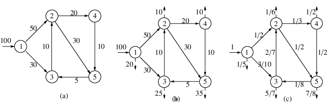
(a) is a hypothetical network (The letter in each node is its index). The black node is the root, the numbers besides edges stand for flows, the dashed lines represent dissipations; (b) shows the , values being denoted inside and beside node respectively by our method; (c) is a spanning tree of (a), the numbers inside and beside vertex are and values calculated by Garlaschelli’s method; (c) is the implicated flow network of (c), the numbers beside edges are flux
Figure 1(a),(c) shows how Garlaschelli’s approach can be applied to a hypothetical flow network (a) to calculate and for each node. At first, a spanning tree (Figure 1 (c)) is constructed from the original network (Figure 1 (a)) by cutting edges. That way, each sub-tree rooted from any can be viewed as a sub-system of the spanning tree. is the total number of nodes involved in this sub-tree and is the summation of s for each node in this sub-tree. Finally, the universal allometric scaling relationship of s and s, with an exponent around , was found for all food webs according to Garlaschelli et al. (2003).
Garlaschelli’s method was inspired by Banavar et al. (1999)’s model to explain the Kleiber’s law. The spanning tree is simply Banavar’s optimal transportation network. Thus, energy flows into the whole system from the root along links of the network to all nodes. Suppose that each node would consume 1 unit of energy in each time step. A flux with 1 unit representing the energy consumption by each node should then be added to the original spanning tree Figure 1(c). In Figure 1(d), the energy dissipation by each node is added as a dotted line(Banavar et al., 1999). As a result, of each node is the throughflow of this node. is the total throughflows of the sub-tree rooted from . Essentially, calculation of allometric scalings using Garlaschelli’s approach is based on this weighted flow network model(Zhang and Guo, 2010).
2.2 Ecological Network Method
We will extend Garlaschelli’s method directly on the original weighted network without cutting edges (e.g. Figure 1). But the key question is how to calculate and for general flow network?
According to the flow network interpretation of Garlaschelli’s method in Figure 1 (d), is the energy flux intake by node which is equals to the total out flows from due to the flow balance condition. Thus, this concept can be extended to any flow network by defining as the throughflow of node . However, defining is not as simple as because we don’t have the sub-system concepts if the considered network is not a tree.
To understand what does mean in Garlaschelli’s method based on the flow network picture (Figure 1 (d)), we suppose to do the following hypothetic experiment. Assume a large number of particles are flowing along the network (Figure 1 (d)), and all particles whenever passing by any node, say b, will be attached a label, say “b”. This trace marker will not be erased forever unless the particle flows out of the network. Then, we found in Figure 1 (c) is just the total number of labeled particles by “b” still being trapped in the whole network. This trace marker experiments can be also applied to other nodes independently and separately by attaching different labels so that all s can be calculated by counting the number of particles who used to pass node .
Actually, this understanding can be extended to any flow network no matter if it is a tree or not(Zhang and Guo, 2010). Although counting the number of labeled particles in the real network is difficult, we can do this calculation directly by Markov chain technique thanks to the ecological network analysis method developed by Patten et al. As long as the flow network is in the steady state so that all flows distributed on edges are stable, a fixed value can be calculated according to the flow structure.
Suppose the flux matrix of the original network is , in which each entry stands for the flux from to . Two special nodes and ( is the total number of species) representing source and sink are contained in this matrix as the first(last) in columns(rows). We define of as,
| (1) |
That is the throughflow of species in ecological network analysis(Ulanowicz, 1997).
To calculate , we should convert the original flux matrix into a Markov chain in which each element is defined as for all . Notice that the Markov chain is normalized (i.e. ) only if the original flux matrix is balanced, i.e.,
| (2) |
This requirement is always satisfied by most empirical ecological networks. The webs not satisfying this condition will be balanced by the method mentioned in Appendix A. Thus, can be calculated as,
| (3) |
where, is the element in matrix , which is called fundamental matrix(Fath and Patten, 1999; Ulanowicz, 2004) and defined as,
| (4) |
where, is the identity matrix. According to the ecological network analysis method, is just the total number of particles that used to pass node (see Appendix B).
Then, we can calculate values for all nodes in the flow network to test the following allometric scaling law,
| (5) |
Where, is the allometric exponent that will be mainly discussed in the following sections.
3 Results
3.1 Description of Data Set
The 19 ecological flow networks in different habitats are studied(Table 1). The networks are obtained from the online database11 1 http://vlado.fmf.uni-lj.si/pub/networks/data/bio/foodweb/foodweb.htm. Most of these networks in this database are from the published papers(Almunia et al., 1999; Baird and Ulanowicz, 1989; Baird et al., 1998; Hagy, 2002; Ulanowicz, 1986; Monaco and Ulanowicz, 1997; Christian and Luzkovich, 1999). In Table 1, we list the name, the number of nodes () and the number of edges () of these networks. In which, the nodes are living species and also non-living compartments (e.g., DOC, POC), the weighted links are energy flows whose values vary in a large range because the units and time scales of the measurements are very different. The source node and sink node are the “input” node and the combination of “respiration” and “output” nodes in the original data respectively. The dissipative flux of each node is just the flow from to which can be read from the data directly. Most ecological flow networks are balanced already (condition Equation 2), few imbalanced networks are balanced by the approach mentioned in Appendix A.
and are the total numbers of nodes and edges respectively, all networks are sorted in decreasing order of Food web Abbre. Florida Bay, Dry Season Baydry 126 2102 1.010 0.995 0.915 0.949 Florida Bay, Wet Season Baywet 126 2071 1.020 0.994 0.917 0.953 Mangrove Estuary, Dry Season Mangdry 95 1462 1.010 0.997 0.978 0.983 Everglades Graminoids, Wet Season Gramdry 67 863 1.030 0.999 0.973 0.997 Everglades Graminoids, Wet Season Gramwet 67 863 1.020 0.999 0.977 0.998 Cypress,Dry Season CypDry 69 639 0.998 0.996 0.957 0.949 Cypress,Dry Season CypDry 70 554 0.998 0.996 0.967 0.949 Cypress,Wet Season CypWet 69 630 0.997 0.997 0.965 0.988 Mondego Estuary -Zostrea site Mondego 44 401 1.010 0.999 0.979 0.997 St. Marks River (Florida) StMarks 52 349 1.020 0.980 0.985 0.950 Lake Michigan Michigan 37 210 1.010 0.999 0.995 0.999 Narragansett Bay Narragan 33 194 1.010 0.991 0.813 0.942 Upper Chesapeake Bay in Summer ChesUp 35 203 1.050 0.997 0.952 0.991 Middle Chesapeake Bay in Summer ChesMiddle 35 195 1.040 0.996 0.851 0.761 Chesapeake Bay Mesohaline Net Chesapeake 37 160 0.994 0.997 0.985 0.985 Lower Chesapeake Bay in Summer ChesLower 35 163 1.050 0.997 0.926 0.971 Crystal River Creek (Control) CrystalC 22 107 1.040 0.997 0.959 0.995 Crystal River Creek (Delta Temp) CrystalD 22 83 1.040 0.998 0.963 0.996 Charca de Maspalomas Maspalomas 22 82 0.956 0.966 1.150 0.737 Rhode River Watershed - Water Budget Rhode 18 54 0.828 0.866 1.200 0.963
3.2 Allometric Scaling Law
We found all the ecological flow networks possess the allometric scaling pattern significantly as an example shown in Figure 2. Their allometric exponents s with the values of are listed in Table 1. We see that the values of are larger than for all food webs except CrystalC, CrystalD and Rhode whose scales are very small (). All of exponents fall into the interval , most of them are larger than a little.

There are only few points in the inset of the lower figure because many nodes in the null model are not balanced and their dissipations are set to zeros
To test if the allometric scaling pattern is significant compared to random flow networks, we built a null model in which the numbers of nodes and edges are kept, all links are re-connected randomly and all flows on edges are also randomly assigned on the interval evenly, where is the maximum flux of the original network. From the inset of first row in Figure 2, we see the null model network doesn’t show the allometric scaling law. We also try to compare the empirical flow networks with other null models. Some of them are obtained by keeping the topology unchanged but randomly assigning the weights, some of them are obtained by just shuffling the weights among edges, all the details of these null models are presented in the Appendix C.
Among these null models, we found the ones keeping weights information have similar allometric scaling exponent as the the empirical food webs. As a result, we know that it is the flow distribution but not the topological structure of the network that is the key ingredient to the allometric scaling exponents. However, to study all possible flow distributions which can affect the final allometric law is impossible because there are hundreds of flows which can be adjusted for an empirical food web. What is the most important aspect? We found the dissipative flux is the key to the allometric exponent.
3.3 Dissipation Law
In ecology, dissipation of a species has different forms such as respiration, excretion, egestion, natural and predatory mortality and so forth(Straškraba et al., 1999). In our data, the dissipative flow is mainly respiration. We can understand the dissipation of a species in an ecological flow network as the flows out of the network, i.e., . It is comprehensible that this output flow increases with the total throughflow of the focus species. But it is not obvious that for most collected ecological flow networks the growth of dissipation along different species is slower than the growth of throughflow. A sub-linear relationship between dissipation and throughflow of each species is hold per se,
| (6) |
where, the exponent in Equation 6 is called dissipation law exponent which can be estimated from the data. Its values for different networks are also listed in Table 1. We see all the values are smaller than 1 except Maspalomas and Rhode networks. The lower plot in Figure 2 shows the dissipation scaling law for Mondego flow network as an example.
3.4 Relationship Between and

The blue dashed line is the curve for the original flow networks, and the solid red one is for the adjusted networks based on the same network structure and the dissipation law according to flow adjusted algorithm (see main text)
Because both and are indicators for the whole flow network, to see how these two numbers correlate each other, we can simply plot different s against s across all the collected empirical flow networks(see the blue dotted curve in Figure 3). Although a general trend that decreases with can be observed, it is not significant due to three major reasons. First. The number of sample points is too small to show clear relationship. Second, most of data points are concentrated in the circled area since all s and s are of similar values for all networks. Finally, the original exponents are noisy so that the values fluctuate in the circled area.
To understand how depends on for a given flow network structure as well as to avoid the problems mentioned in the previous paragraph, we invent a specific technique called “Flow Adjusting Algorithm (FAA)”. This algorithm enables us to perturb the given flow network structure as little as possible and simultaneously observe how changes by tuning . Concretely, for a given original flow network , we keep the network topology, the relative importance of each influx unchanged (That is, ), meanwhile adjust the flow distributions on each edge to obtain a new flow network such that:
(1) The given dissipation law, i.e., , is hold for every node in , where is a given exponent which can be tuned. We will study how impacts the allometric scaling law;
(2) The flux balance condition, i.e., must be kept for each node ;
In this way, we can perturb the flow structure of the original network to obtain the expected dissipation law, and to observe how exponent affects exponent . The details of the “flow adjusting algorithm” will be introduced in Appendix D. Figure 4 shows the dependence of and on the perturbed networks by MAA based on the original Mondego flow network, randomized Mondego flow network (based on Mondego’s topology but assign flows randomly) and simulated networks by Niche model(Williams and Martinez, 2000). We observe the allometric scaling exponent decreases with the dissipation law exponent in a similar manner no matter the original network structures are. However, the concrete shapes of the curves between and change with the network structures. For networks generated by Niche model, decreases with in a slower speed when the connectances are higher (blue triangles versus purple triangles and yellow diamonds versus green diamonds). As a result, the dissipation law exponent but not the structure is the major feature to affect the allometric exponent. But we cannot conclude the topological structure has no influence on the allometric exponents, we will discuss this problem further in Appendix E.

The black and red curves are the original and randomized flow networks of Mondego respectively. The randomized flow network keeps the topological structure of Mondego network but assign flux randomly. Other dashed curves are for networks generated by Niche model with different number of nodes (100 or 50) and connectances (0.4 or 0.1), as well as the random assigned flows(Williams and Martinez, 2000). MAA is applied on all these flow networks to obtain the relationships between and . All the exponents are the average results of 50 random experiments. The red star shows the original position of dissipation law exponent (0.980) and allometric exponent (1.012) of Mondego network. While the red circle corresponds to the combination of the original dissipation law exponent (0.980) and the adjusted allometric exponent (1.011) by FAA on Mondego network.
In Figure 4, the red circle in the middle of the black curve stands for the combination of the dissipation law exponent of the original Mondego network and the allometric exponent of the adjusted flux matrix by the flow adjusting algorithm. While, the red star corresponds to the original exponents of Mondego network both for and . We see these two points almost overlap together which means the original Mondego food web satisfies two conditions:
(1) dissipation law is significant for the original ;
(2) the balance Equation 2 is obeyed exactly.
However, for other empirical networks, the perturbed result of allometric exponent is not identical to the original one exactly on the given original dissipation law exponent because either the flux balance condition is violated or the dissipation scaling law is not significant (see Appendix F).
By adjusting the flows on all empirical flow networks with the fixed original dissipation law exponent , we can eliminate noise in raw data because we conform the network to be flow balanced and satisfy the given dissipation law. The red solid curve in Figure 3 shows the clear dependence of and of all the empirical flow networks. We see the decreasing trend of the blue dashed line standing for the original exponents is not as obvious as the red one representing the adjusted results. Therefore, the two conditions listed before cannot be satisfied by the some original ecological networks perfectly.
4 Discussion
4.1 Transportation Efficiency or Inequality of Species Impact?
Previous studies explained the allometric scaling exponent as the transportation efficiency of the network and is bound in between 1 (a star network, the most efficient tree) and 2 (a chain, the most inefficient tree).
However, in our study, the allometric scaling exponent is not bound in the interval , therefore, we should give a new explanation for the exponent . The key problem is to understand the indicator .
In Banavar’s model and Garlaschelli’s method, they understand as a cost of energy transportation for the sub-tree rooted from . In this way, the energy flows on the redundant links (loops or cross-leveled links) except the ones in the spanning tree are wasted. Nevertheless this interpretation can hardly generalize to flow networks because (1) the wasted energy in the weighted networks can be measured as dissipation of each node but not the weight of edges; (2) all energy links should be considered because they all contribute to the whole flow distribution.
According to the particle coloring experiment mentioned in Section 2, we can understand as the total impact of to the whole network along all flow pathways(Vitali et al., 2011) because it is the total number of particles who used to pass at least one time. Thus, as increases, more other nodes will be affected by the particles used to pass , the direct and indirect influences of will increases. This understanding toward can be extended to any flow network.
As the species climbs up along the energy throughflow gradient , its total impact also increases with a relative speed according to the allometric scaling law . Therefore, the important nodes (with larger ) may have much greater power (total impact ) in the networks with larger exponent than those networks with smaller exponents. For example, we have two networks with 4 nodes. They have the same throughflow distributions, e.g., , but different exponents and , therefore different distributions . The most important node (with largest ) in the second network may have much greater impact () to the whole network than the first one (). Hence, the inequality of the species impact of the second network is larger than the first one. In short, the allometric exponent measures the inequality of species impact.
This new interpretation is compatible with the previous one. For Garlaschlli’s spanning trees, the most inequable tree with a given root is a chain but the most equable one is a star.
4.2 Dissipation and Inequality
According to the new interpretation of allometric exponent and the discovery of the relationship between dissipation and allometry, we can obtain a whole picture: the networks may become more equable by dissipating more energy on larger nodes since the impacts of high flux nodes are weakened. In the networks with , the dissipation flow per throughflow of each node increases, the energy invested to the whole network decreases with the size of node, the network is more decentralized. On the other hand, if is smaller than 1, the dissipating flux scales to the throughflow with a smaller relative speed. So the large nodes may input more energy on the whole network to obtain much more powerful impact on other nodes, the networks are more centralized.
However, an interesting unexplained fact is the allometric exponents of empirical ecological networks are all close to 1. They are neither inequable nor equable. We guess this exponent should be an optimal result by some unknown factors. This will be left for future studies.
In summary, this paper generalize the universal allometric law to the ecological flow networks and discover that the major factor to the allometric exponent is , the dissipation law exponent. By reinterpreting allometric exponent as the inequality of species impacts, we build a connection between network structure and the thermodynamic constraint. This connection is very important deserving more attention.
References
- Allesina et al. (2008)
Allesina, S., Alonso, D., Pascual, M., 2008. A general model for food web
structure. Science 320 (5876), 658–661.
URL http://www.sciencemag.org/cgi/content/abstract/320/5876%/658 - Allesina and Bodini (2004)
Allesina, S., Bodini, A., 2004. Who dominates whom in the ecosystem? energy
flow bottlenecks and cascading extinctions. Journal of Theoretical Biology
230 (3), 351–358.
URL http://www.sciencedirect.com/science/article/pii/S00225%19304002620 - Allesina and Bodini (2005) Allesina, S., Bodini, A., 2005. Food web networks: Scaling relation revisited. Ecol. Complex. 2, 323–338.
- Almunia et al. (1999)
Almunia, J., Basterretxea, G., Aristegui, J., Ulanowicz, R., 1999.
Benthic-pelagic switching in a coastal subtropical lagoon. Estuarine, Coastal
and Shelf Science 49 (3), 363–384.
URL http://www.sciencedirect.com/science/article/pii/S02727%71499905036 - Baird et al. (1998)
Baird, D., Luczkovich, J., Christian, R., 1998. Assessment of spatial and
temporal variability in ecosystem attributes of the st marks national
wildlife refuge, apalachee bay, florida. Estuarine, Coastal and Shelf Science
47 (3), 329–349.
URL http://www.sciencedirect.com/science/article/pii/S02727%71498903602 - Baird and Ulanowicz (1989) Baird, D., Ulanowicz, R. E., 1989. The seasonal dynamics of chesapeake bay ecosystem. Ecol. Monogr. 59, 329–364.
- Banavar et al. (1999) Banavar, J., Maritan, A., Rinaldo, A., 1999. Size and form in efficient transportation networks. Nature 399, 130–132.
- Bersier and Sugihara (1997)
Bersier, L.-F., Sugihara, G., 1997. Scaling regions for food web properties.
Proceedings of the National Academy of Sciences of the United States of
America 94 (4), 1247–1251.
URL http://www.pnas.org/content/94/4/1247.abstract - Brown and Gillooly (2003) Brown, J., Gillooly, J., 2003. Ecological food webs: High-quality data facilitate theoretical unification. Proc. Natl. Acad. Sci. U. S. A. 100 (4), 1467–1468.
- Camacho and Arenas (2005)
Camacho, J., Arenas, A., Jun. 2005. Food-web topology: Universal scaling in
food-web structure? Nature 435 (7044), E3–E4.
URL http://www.nature.com/nature/journal/v435/n7044/abs/nat%ure03839.html - Cattin et al. (2004) Cattin, M., Bersier, L., Richter, C., Baltensperger, R., Gabriel, J., 2004. Phylogenetic constraints and adaptation explain food-web structure. Nature 427, 835–839.
- Christian and Luzkovich (1999) Christian, R. R., Luzkovich, J. J., 1999. Organizing and understanding a winter’s seagrass foodweb network through effective trophic levels. Ecological modelling 117 (1), 99–124.
- Cohen et al. (1990) Cohen, J., Briand, F., Newman, C., 1990. Community Food Webs: Data and Theory (Biomathematics Vol. 20). Springer, Berlin.
- Dreyer (2001) Dreyer, O., 2001. Allometric scaling and central source systems. Phys. Rev. Lett. 87, 038101.
- Fath et al. (2001) Fath, B., Patten, B., Choi, J. S., 2001. Complementarity of ecological goal functions. J. Theor. Biol. 208, 493–506.
- Fath and Patten (1998) Fath, B. D., Patten, B., 1998. Network synergism: emergence of positive relations in ecological systems. Ecol. Model. 107, 127–143.
- Fath and Patten (1999) Fath, B. D., Patten, B. C., 1999. Review of the foundations of network environ analysis. Ecosystems 2, 167–179.
- Finn (1976) Finn, J. T., 1976. Measures of ecosystem structure and function derived from analysis of flows. J. Theor. Biol. 56, 363–380.
- Frank and Murrell (2005) Frank, F., Murrell, D., 2005. A simple explanation for universal scaling relations in food webs. Ecology 86 (12), 3258–3263.
- Garlaschelli et al. (2003) Garlaschelli, D., Caldarelli, G., Pietronero, L., 2003. Universal scaling relations in food webs. Nature 423, 165–168.
- Hagy (2002) Hagy, J., 2002. Eutrophication, hypoxia and trophic transfer efficiency in chesapeake bay. Ph.D. thesis, University of Maryland at College Park, College Park, Maryland.
- Hannon (1973) Hannon, B., 1973. The structure of ecosystems. J. Theor. Biol. 41, 535–546.
- Hannon (1986) Hannon, B., 1986. Ecosystem control theory. J. Theor. Biol. 121, 417–437.
- Higashi (1986) Higashi, M., 1986. Extended input-output flow analysis of ecosystems. Ecol. Model. 32, 137–147.
- Higashi et al. (1993) Higashi, M., Patten, B. C., Burns, T. P., 1993. Network trophic dynamics: the modes of energy utilization in ecosystems. Ecol. Model. 66, 1–42.
- Kleiber (1932) Kleiber, M., 1932. Body size and metabolism. Hilgardia 6, 315–353.
- Krause et al. (2003) Krause, A. E., Frank, K. A., Mason, D. M., Ulanowicz, R. E., Taylor, W. W., 2003. Compartments revealed in food-web structure. Nature 426, 282–285.
- Levine (1980) Levine, S., 1980. Several measures of trophic structure applicable to complex food webs. Journal of Theoretical Biology 83 (2), 195–207.
- Monaco and Ulanowicz (1997) Monaco, M. E., Ulanowicz, R. E., 1997. Comparative ecosystem trophic structure of three U.S. mid-atlantic estuaries. Marine Ecology Progress Series 161, 239–254.
- Odum (1983) Odum, H., 1983. System Ecology. John Wiley & Sons Inc.
- Odum (1988) Odum, H. T., 1988. Self-organization, transformity, and information. Science 242, 1132–1139.
- Pascual and Dunne (2005) Pascual, M., Dunne, J. A., Dec. 2005. Ecological Networks:Linking Structure to Dynamics in Food Webs: Linking Structure to Dynamics in Food Webs. Oxford University Press.
- Patten (1981) Patten, B. C., 1981. Environs: the superniches of ecosystems. American Zoologist 21, 845–852.
- Patten (1982) Patten, B. C., 1982. Environs: relativistic elementary particles or ecology. American Natualist 119, 179–219.
- Patten (1985) Patten, B. C., 1985. Energy cycling in the ecosystem. Ecol. Model. 28, 1–71.
- Pimm (2002) Pimm, S., 2002. Food webs. University Of Chicago Press.
- Rodriguez-Iturbe and Rinaldo (1997) Rodriguez-Iturbe, I., Rinaldo, A., 1997. Fractal River Basins. Chance and Self-Organization. Cambridge University Press,, Cambridge.
- Straškraba et al. (1999) Straškraba, M., Jørgensen, S. E., Patten, B. C., 1999. Ecosystems emerging: 2. dissipation. Ecological Modelling 117 (1), 3–39.
- Sugihara et al. (1989) Sugihara, G., Schoenly, K., Trombla, A., Jul. 1989. Scale invariance in food web properties. Science (New York, N.Y.) 245 (4913), 48–52, PMID: 2740915.
- Szyrmer and Ulanowicz (1987) Szyrmer, J., Ulanowicz, R. E., 1987. Total flows in ecosystems. Ecol. Model. 35, 123–136.
- Ulanowicz (1986) Ulanowicz, R. E., 1986. Growth and Development, Ecosystems Phemomenology. Springer-Verlag, New York.
- Ulanowicz (1997) Ulanowicz, R. E., 1997. Ecology, the Ascendent Perspective. Columbia University Press, New York.
- Ulanowicz (2004) Ulanowicz, R. E., 2004. Quantitative methods for ecological network analysis. Comput. Biol. Chem. 28, 321–339.
- Vitali et al. (2011) Vitali, S., Glattfelder, J. B., Battiston, S., 2011. The network of global corporate control. PLoS ONE 6, e25995.
- West et al. (1999) West, G., Brown, J., Enquist, B., 1999. The fourth dimension of life: Fractal geometry and allometric scaling of organisms. Science 284, 1677–1679.
- West et al. (1997) West, G., Brown, J. H., Enquist, B. J., 1997. A general model for the origin of allometric scaling laws in biology. Science 276, 122–126.
- Williams et al. (2002) Williams, R. J., Berlow, E. L., Dunne, J. A., Barabasi, A., Martinez, N. D., 2002. Two degrees of separation in complex food webs. Proc. Natl. Acad. Sci. U. S. A. 99 (20), 12913–12916.
- Williams and Martinez (2000) Williams, R. J., Martinez, N., 2000. Simple rules yield complex food webs. Nature 404, 180–183.
- Zhang and Guo (2010)
Zhang, J., Guo, L., 2010. Scaling behaviors of weighted food webs as energy
transportation networks. Journal of Theoretical Biology 264 (3), 760–770.
URL http://arxiv.org/abs/1003.4573
Appendix
Appendix A Balancing A Flow Network
For most of empirical ecological flow networks, the flux matrix is balanced which means holds for each . However, some empirical networks and most artificial networks (e.g. random network) are imbalanced. Therefore, we should balance the given network artificially so that the ecological network analysis methods can be applied.
Suppose for node . We can add an edge with the flux , to connect node to or . If , the direction of this artificial edge is from to . If , the direction is from to . We can do this process for all nodes except and to balance the whole network.
Appendix B Explanation on Calculation by an Example Network
In this Section, we will explain why the number of particles labeled by node can be calculated as Equation 3 through an example network (see Figure 5).
(a). The original flow network which is imbalanced; (b). The balanced network; (c). The corresponding Markov chain
Notice that the original network is imbalanced, we should balance it at first by the approach mentioned in the last section. Then, the balanced network can be converted to a Markov chain simply through being normalized by the output flow of each node as shown in Figure 5 (c). We know any element in Markov matrix stands for the transfer probability of a particle from to given that the particle locates already and the whole network is in the steady state. And any element in matrix is the probability of a particle locating on at first and transfer to along all possible pathes after steps. All these information is aggregated in the fundamental matrix because,
| (7) |
We should be careful to give an intuitive explanation on because its element does not stand for probability anymore although the element in each term is the transitional probability. We can write down the fundamental matrix for our example network (by ignoring the elements for source and sink ),
| (8) |
Notice that the elements on the diagonal are larger than 1, so they cannot be interpreted as probability simply.
Next, we will calculate the first passage flow to any node . Here, is defined as the number of particles passing in the first time. If all the particles passed are labeled, then is the number of particles passing and unlabeled by it at each time. This quantity can be calculated as,
| (9) |
For example, the first passage flow of node 4() can be calculated as,
| (10) |
Actually, each term of Equation 9 is the first passage flow from node to , that is the number of particles that have visited (in whatever time) and finally arrive at in the first time along all possible flow pathways. By dividing by the term to derive first passage flow one avoids duplicate counting the particles who have visited (Higashi et al., 1993).
Because at each time, there are totally unlabeled particles will pass and be unlabeled by “b”, thereafter, new “b” particles will be injected to the system and will flow to other nodes along pathways. Then, at given time step, there are totally labeled particles just injected , and labeled particles injected one time step ago, and labeled particles injected two time steps ago,…, labeled particles injected time steps ago, and so forth.
Hence, the total number of labeled particles that flowing in the whole network at each time, being defined as , is just the summation of the labeled particles being attached 1 time step ago, 2 time steps ago,…, and so on. Therefore, we can calculate as:
| (11) | ||||
For example, of node 2 in the example network is calculated as:
| (12) |
Appendix C Null Models
To test if the allometric scaling law is a significant pattern in empirical ecological network, we designed four kinds of null models based on empirical networks.
Null Model 1 (NM1): We only keep the total number of nodes and edges as the original empirical flow network, and build random connections, assign random weights for each edge. The weights are evenly distributed on the interval , where is the maximum flux in the original network. In this way, the topology and flow distribution are destroyed.
Null Model 2 (NM2): The connections are kept, the weights are randomly assigned for each edge. In this model, weights are also randomly sampled from the interval . In this way, only the flow distribution is destroyed.
Null Model 3 (NM3): Keep the connections, shuffle the weights on edges. That is, we keep the topology and weights distribution but permute these weights on edges. In this way, the flow distribution is not changed but the correlations between flows are destroyed.
Null Model 4 (NM4): Keep the weights, the number of edges, but randomly assign the weighted connections between any pair of nodes. In this way, the flow distribution is kept, but their correlations and the network topology are destroyed.
For each original ecological flow network, we built four null models. The flux matrix of the null models is imbalanced normally, then we should balance it by the approach mentioned in Section A, after that we calculate their and for each node and derive the allometric scaling law pattern.

Figure 6 shows the allometric scaling relationships for s and s for null models of Mondego network. From this figure, we know NM3 and NM4 have more similar pattern as the original networks than NM1 and NM2, which means the flow distribution is more important than topology for allometric scaling. Although NM3 and NM4 have significant scaling pattern, their exponents s are smaller than the one of the original Mondego network. Therefore, NM3 and NM4 cannot reproduce the main characters of the original network.
Furthermore, we generate 50 networks for each null model on each empirical flow network collected. The average values of s are compared to the original ones in Figure 7. From this figure, we can see that the exponents of NM3 and NM4 are more close to the original networks with less fluctuations. That means the weights information is more important than the structures and the weight correlation play a minor role on allometric exponents. Although NM3 and NM4 have similar exponents as the original networks, all their values are smaller than the ones of the original networks.

All the empirical flow networks are sorted in the order of Table 1 along the horizontal axis(the left most network has largest number of nodes). The data points and error bars in all null models stand for the average numbers and standard deviations of exponents of 50 experiments.

The dissipation laws are calculated for the artificial balanced networks to compare with the allometric laws in Figure 6
Further studies on the dissipation laws of these null models can explain the patterns shown in Figure 7. From Figure 8, we observe that most networks do not have obvious dissipation scaling law. However, we can observe the obvious straight lines formed on the ceiling of data clouds for NM3 and NM4, although lots of scatter points are below them. Actually, the artificial balancing method can account for this phenomenon. Because in NM3 and NM4, all the weights of links are not changed but the connections are destroyed so that the energy influx cannot balance with out flows for lots of nodes, the balanced flows (dissipations) are almost proportional to the original flow. Therefore, before we fit the data clouds by using a line on NM3 and NM4, we actually left the data under the lines as outliers. In this way, we can estimate the right s for NM3 and NM4 which are close to 1. By comparing Figure 8 and Figure 6, we know that the relationship between and is also suitable for these null models.
Appendix D Flow Adjusting Algorithm
In the main text Section 3.4, we apply the so called “Flow Adjusting Algorithm” to perturb the original flow network. In this section, we will introduce the detailed steps of this method.
The main purpose is to conform the adjusted flow network to satisfy two conditions (1) dissipation law with given exponent, and (2) flow balance requirement without changing the topology and relative weight of each flow. Or we can express it as a mathematical problem: to find a solution of the following equations system.
| (13) |
Where and are given constants, s and s are variables.Therefore we have totally equations but variables. For normal flow networks, , so we should have infinite solutions to the Equation 13. However, solving these equations are hard because they are non-linear.
The flow adjusting algorithm is an approximate algorithm to solve these equations. At first, we have a nodes set , a set of stop criterions. Initially, we set time step , , the flux matrix as the original flow network , where the superscripts on and are the current time step. The algorithm will repeat the following steps:
(1). For any node in , the algorithm needs the current out flows from , . Solve the equation for :
| (14) |
i.e., the new total influx to .
(2). Assign to all incoming edges to proportionately, set
| (15) |
and
| (16) |
(3). Add all input nodes s of into set and delete from ;
(4). Set , repeat the previous steps until the stop criterions, which include the total running time being smaller than a given number, the dissipation law exponent and for the new flux matrix being close to the wanted values, are satisfied.
This algorithm works once the network is connected (which means there is at least one path from to every node ). For most of networks, the algorithm can converge to a network pertaining the significant dissipation law on the given exponent. However, it may oscillate on some topologies, especially for random networks. Further approvement of this algorithm will leave for the future works.
Appendix E and Relationships for Modeled Networks
To better understand how correlates with , we will study several special modeled networks in this section.
E.1 Minimum Spanning Tree
We now consider a special case: minimum spanning tree introduced by Frank and Murrell (2005). By controlling two parameters and , we can generate variant trees with different basal species ratio(controlled by ) and maximum trophic level (controlled by ).
The tree’s construction process is as follows. Let’s consider an ecological community with different species, in which a hypothetic food web (tree structure) will be built. At first, we select species as the basal species at the first trophic level. And at each time, a new species is added to the minimum spaning tree. will select a node as its unique prey according to the probability:
| (17) |
where, is ’s trophic level + 1 (i.e., the depth of in the tree), is the set of species which are already in the spanning tree, and is a parameter to control the attachment preference of the new node on depth. If is large, the new node may attache to the position being close to the root.
After a tree is constructed, we will assign random values in the original flux matrix and then apply the “Flow Adjusting Method” on it. In this way, we can investigate the influence of both tree’s structure ( and ) and dissipation exponent on the allometric scaling exponent .

For each combination of parameters, we generate 10 minimum spanning trees to get the average value of . The species number in all simulations
From Figure 9, we found at first both the dissipation law and network structure can affect the allometric scaling. However, depends more on than and because will change with intensively. When is given, we can observe the similar trend of depends on and as the results introduced by Frank and Murrell (2005).
Interestingly, when is set to be 0, each node’s dissipation is a constant, this corresponds to Garalaschelli’s approach’s assumption (see Figure 1(d)). And the exponent derived by our algorithm is exactly same as the result derived by Garlaschelli’s approach on the same tree. And the dependence of on and is same as (Frank and Murrell, 2005). So, our method can recover Garlaschelli’s method on spanning trees.
E.2 Random Network
We also test the “Flow Adjusting Algorithm” on random networks. The results are shown in Figure 10.

All s are averaging for 10 random networks
We only show the results of random networks with 50 nodes but different number of edges because the FAA is hardly to converge on the random networks with large number of edges. When the algorithm cannot get a final result after a given number of time steps (200), we have to regenerate a new random network with the same number of nodes and edges. It is interesting to observe that when the number of edges is large, the responding curve of on is very different from the ones in Figure 3. s are always very small, where almost gets a peak when approaches . Therefore, we know the topological structure does affect the allometric exponent.
Furthermore, we generate random networks based on a minimum spanning tree by adding additional edges randomly. When , the network is an MST, while when , it is a complete graph. Therefore, we can observe how the corresponding curve of on changes when the network structure changes from a tree to a random network by tuning .

All s are average results of 10 networks, the backbone trees are of the parameters .
From Figure 11, the dependance of on when is different from the random networks with the same connectance but similar to the ones of empirical ecological networks. That is because the former random network is generated based on a minimum spanning tree which can be viewed as its backbone. Therefore, the spanning tree backbone is a key ingredient to the allometric exponent. Additionally, in Figure 11, all the random networks based on spanning tree with different have a peak on when .
According to these experiments, we know both network structure and dissipation law exponent can influence allometric exponents. But the exponent is more important than the structure. And the shape of backbone spanning trees can change the shape of the relationship between and .
Appendix F Flow Adjustment for Empirical Ecological Flow Networks
“Flow Adjusting Algorithm” is applied to collected empirical ecological flow networks as shown in Figure 3 on Mondego as an example. In this section, we will show the results for other networks and discuss the technique details.

Each plot shows results of “Flow Adjusting Algorithm” on two empirical networks (black and blue curves), the red diamond and disk stand for the , combinations for the original exponents and the adjusted results by “Flow Adjusting Algorithm” on the original for the first ecological network; and the green star and square are for the second ecological network.
The basic idea of “Flow Adjusting Algorithm” is to tune various flows on the network until the dissipation law exponent is close to the wanted value. When we apply this method on the empirical ecological networks, we adjust the flows until either (1) the adjusted dissipation law exponent satisfies , where is the wanted exponent and (2) the of the dissipation power law on the adjusted flows should satisfy , where is the Rsquare of the dissipation law for the original flow network; or (3) The running time steps are larger than 500. Because the algorithm may diverge, whence the first requirement may not be satisfied, we have to stop the algorithm within a finite time steps and retrieve one of the best network as the output.
In Figure 12, we show results for applying FAA on all collected ecological networks. The red diamond and green stars are the and combinations for the original networks, and the red disk and green squares stand for the ones for FAA results on the original as the designed exponent. If the original flow network satisfies the dissipation law and flow balance condition perfectly, then the adjusted value should be similar with the value of the original network (which indicates that the red disks(green squares) should overlap with the red diamonds(green stars)). However, we observe that the markers for some networks do not overlap which means the corresponding original networks do not satisfy that two conditions perfectly.

Let’s see Baydry network as an example. Although the original flow network possess a very good dissipation law as shown in the left-top plot in Figure 13, this network is not balanced. Because balance is a basic requirement of the algorithm for allometric scaling law mentioned in Section 3.2, we have to balance Baydry network at first by the method in Section A. However, the balanced flow network always has different dissipation law (compare the left-top plot to the right-top one in Figure 13). Therefore, the original and the one adjusted by FAA are different (The first plot red disk and diamond in Figure 12).
Another example network which is balanced but not be of good dissipation law is Rhode as shown in the left-bottom and right-bottom plots of Figure 13. We observe that the dissipation scaling law is not significant () for Rhode network. Therefore, the original and adjusted exponents do not overlap (The first plot green star and square in Figure 12). Furthermore, FAA cannot obtain a convergent result on Rhode network, that is the reason why the green star and square have different horizontal coordinates.
Because the negative relationship between and is significant only if the flow network satisfies (1) a significant dissipation law and (2) the flows are balanced, we adjust the flows of the empirical networks to conform the dissipation law with the original dissipation law. In this way, we believe the noise contained in original data can be eliminated, so that more exact allometric exponents can be computed. The red solid curve in Figure 3 shows the original exponents and adjusted exponents.