Matrix product states and variational methods applied to critical quantum field theory
Abstract
We study the second-order quantum phase-transition of massive real scalar field theory with a quartic interaction in (1+1) dimensions on an infinite spatial lattice using matrix product states (MPS). We introduce and apply a naive variational conjugate gradient method, based on the time-dependent variational principle (TDVP) for imaginary time, to obtain approximate ground states, using a related ansatz for excitations to calculate the particle and soliton masses and to obtain the spectral density. We also estimate the central charge using finite-entanglement scaling. Our value for the critical parameter agrees well with recent Monte Carlo results, improving on an earlier study which used the related DMRG method, verifying that these techniques are well-suited to studying critical field systems. We also obtain critical exponents that agree, as expected, with those of the transverse Ising model. Additionally, we treat the special case of uniform product states (mean field theory) separately, showing that they may be used to investigate non-critical quantum field theories under certain conditions.
pacs
11.10.Hi, 11.10.Ef, 11.10.Kk, 11.15.HaIntroduction
Quantum field theories (QFT) [1] are extremely good at describing and predicting the behavior of fundamental particles, as demonstrated by the prediction of the Higgs boson over forty years ago and its recent apparent discovery [2]. Very often, however, obtaining predictions from QFT is difficult due, in no small part, to the huge Hilbert spaces they are set in. In many cases, such as quantum electrodynamics (QED), perturbation theory has been used very successfully, yet some important phenomena are not accessible to these methods, notably confinement in quantum chromodynamics (QCD) [3]. Lattice regularizations of QFT’s have been very useful in such cases, often in combination with Monte Carlo numerical techniques. Here, however, the sign problem [4] presents a challenge - not to mention that such simulations often require very large computational resources to produce useful results (see [5], where hadron masses are determined with the help of clusters and a supercomputer).
Meanwhile, the numerical study of lattice systems in one spatial dimension has benefited greatly from the density matrix normalization group (DMRG) method, which has been recognized as a variational method producing approximate ground states that are matrix product states (MPS) [6, 7]. There is a direct link between the dimension of the MPS parameter-space and the amount of entanglement that a state can contain, allowing efficient representation of a great many relevant states [8, 9, 10], in particular ground states and low-lying excited states of gapped systems [11, 12, 13], which all lie in the low-entanglement “corner” of Hilbert space. Recently, other variational techniques have been applied to MPS such as the time-dependent variational principle (TDVP) [14], which permits efficient simulation of dynamics, and a related excitation ansatz for the determination of dispersion relations [15] for translation-invariant systems in the thermodynamic limit.
Given the great successes of MPS and variational methods in studying lattice systems, it is natural to ask whether they can be usefully applied to lattice quantum fields in dimensions, and whether continuum results can be extracted efficiently. A useful test case is -theory which, despite its simplicity, exhibits interesting behavior such as spontaneous symmetry-breaking. It contains a second-order quantum phase-transition in dimensions [16] and is expected to belong to the same universality class as the transverse Ising model [17] so that critical exponents should be the same for both. In fact, DMRG has already shown promise when applied to -theory [18, 19], reproducing the expected critical behavior and obtaining values of the critical parameter close to those of Monte Carlo studies [20, 21, 22].
We use variational methods with MPS to obtain the ground-state field expectation value and low-lying excitation energies of -theory. The scaling of these quantities in parameter-space allows us to locate the critical point and to determine the critical exponents. We begin by introducing QFT and real scalar field theory in section I, showing how it can be put on a spatial lattice and discussing its critical behavior. In section II, we define the uMPS variational class and the corresponding TDVP algorithm and excitation ansatz before detailing our variational conjugate-gradient method for finding ground states. Section III is the main part of this work, in which we apply these techniques to -theory and obtain our estimate for the continuum critical parameter, which we compare with previous results from the literature, as well as values for critical exponents and the central charge. We also separately assess the usefulness of mean-field theory (a special case of MPS) for studying QFT, which is an attractive tool because of the low computational complexity required to estimate physical quantities.
We have kept the software developed for this work intentionally general such that it may be of use to others. It is available under a permissive open-source license [23].
I Quantum field theory
We introduce the basic principles of quantum field theory using the Hamiltonian formulation with real scalar fields as an example, defining interacting -theory both in the continuum and on a spatial lattice. We then discuss its spontaneous symmetry-breaking, which corresponds to a second-order quantum phase-transition in dimensions. The beginning of this section is based partly on lectures on quantum field theory given by Marco Zagermann at Leibniz Universität Hannover in 2010/11 and also on [1].
I.1 Real scalar field without interactions
Quantum fields in Minkowski space-time are quantum systems set in an uncountably infinite-dimensional Hilbert space which can usually be divided naturally into subsystems corresponding to points in momentum space. They can often be constructed from a corresponding classical field defined by a Lorentz-invariant action. The classical field is then quantized in such a way as to produce a consistent Hilbert space and Hamiltonian where Lorentz-invariance and causality are maintained.
As an example, take a classical real scalar field with action
| (1) |
where , and scalar products are defined via the Minkowski metric with the “mostly-minus” signature . We use to denote the spatial part of a Minkowski vector . The integrand is called the Lagrangian density. Stability with respect to a small variation requires that the Euler-Lagrange equations
are satisfied, leading in this case to the equation of motion
where , which is the Klein-Gordon equation. The lack of non-linear field-terms in the equations of motion makes this a free (non-interacting) field. Performing a Fourier transform , we can rewrite the equations of motion as
which has the form of a simple harmonic oscillator with angular frequency . We can thus think of the classical Klein-Gordon field as a set of independent harmonic oscillators, one for each point in momentum space.
To quantize this free scalar field theory, we start from the classical Hamiltonian. The canonical conjugate momentum corresponding to the coordinate is
and, performing a Legendre transformation, the Hamiltonian density is
The coordinate and the momentum obey the Poisson-bracket relationship
where is the -dimensional Dirac delta distribution. The ingredients required for a canonical quantization of the classical theory are now ready. To proceed, we replace the classical phase-space coordinates in the above relations with operators (one for each space-time coordinate) obeying the commutation relation
The field operator is Hermitian because the classical field was real-valued. We now have an operator-valued field where the operators must obey the Klein-Gordon equation. The harmonic oscillator picture of the classical field suggests attempting to write solutions in terms of quantum harmonic oscillators. Making the same move to momentum space as before, we can write a general solution as a superposition of plane waves using Fock-space creation and annihilation operators and
where and . The Hilbert space contains the vacuum and countably infinite excited states for each momentum . Using , we can write the Hamiltonian as
where the second term does not annihilate the vacuum, leading to an infinite vacuum energy contribution. This is perhaps not too surprising: We are summing up an infinite number of ground state energies, one for each Fourier mode, each of which is the energy contained within an infinite volume of space. Since it is energy differences that are observable, and not absolute energies, this infinite contribution should not cause any problems. A general eigenstate has energy (ignoring the infinite vacuum contribution) and is also a momentum eigenstate with momentum , where the momentum operator can be obtained via the classical theory as the conserved quantity associated with spatial translations (using Noether’s theorem). The field operator (in the Heisenberg picture) acts on the vacuum to create a superposition of momentum eigenstates resulting in a particle localized at the space-time coordinate .
A quantity that turns out to be very useful is the two-point correlation function , which can be interpreted as the probability of a particle created at point propagating to point (or vice-versa, depending on the time-coordinates). For this reason it is also called the propagator. It has the form
A related quantity is the Feynman propagator, which is defined as
| (2) | ||||
| (3) |
where denotes the time-ordered product and the relation to can be found using contour integration, with the infinitesimal shift providing a prescription for treating the poles. is a Green’s function of the Klein-Gordon equation
The integrand of has poles given by the mass parameter at . For an interacting theory, the poles no longer correspond to the mass parameter , but are shifted away from this point due to self-interaction. The shifted poles of the propagator then correspond to the physical mass of a particle whereas the “bare” parameter does not. That the poles of the propagator correspond to the particle mass can be seen by inserting the identity, written in terms of the (unspecified) eigenstates of the Hamiltonian (interacting or not) and the momentum operator, into the expression for the propagator. The identity thus formed is
where is the vacuum, is the zero-momentum state boosted to momentum , and with being the mass or energy of . Evaluating leads to the Källén-Lehmann spectral representation of the Feynman propagator (see section 7 of [1])
where is the Feynman propagator with mass-parameter (instead of ) and
| (4) |
is the spectral density. We drop the term, since it adds at most a constant term to the propagator.
Given that the theory contains single-particle states, the spectral density contains a pole at , where is the mass of a single particle, followed by a gap before further excitations appear. In this case, the Feynman propagator can be separated into a one-particle contribution and the rest. With a Fourier transform we have
where is a real number coming from the factors. The single-particle term has a pole at , with the other terms showing up at higher momenta.
I.2 Interacting fields
So far, we have considered the quantized free scalar field, whose solutions are plane-waves. A free (non-interacting) field is, however, not directly relevant to physics, since a lack of coupling implies a lack of measurable consequences. We can introduce interactions by adding a term to the Lagrangian density that leads to non-linear equations of motion. An example for real scalar field theory, and the case we focus on in this paper, is the quartic interaction term
where is the coupling constant, or the strength of the interaction. The resulting theory is often referred to simply as “-theory”. Its equation of motion is
| (5) |
which no longer has simple plane-wave solutions. Since interacting theories are generally difficult or impossible to solve analytically, other approaches such as discrete (lattice-based) numerical simulation or perturbation theory are needed. The perturbative approach is used to study scattering, where it is assumed that the incoming and outgoing states far from the scattering location, called asymptotic states, can be described by the non-interacting field theory. Scattering is then represented by a unitary operator, the “S-matrix”, relating the incoming and outgoing states. Elements of the S-matrix can be calculated perturbatively in powers of the coupling constant. The individual terms in the expansion have a regular form and can be conveniently represented using Feynman diagrams.
Since, for this work, we perform numerical simulations on a lattice, we do not go into perturbative calculations in detail. As mentioned above, the perturbative calculation of the propagator in an interacting theory reveals a shift of the pole mass away from the bare mass parameter , resulting in a different, “dressed” physical mass . The mass shift is due to the interaction of the field with itself, which can involve modes of any momentum. In fact, taking all possible momenta into account, the shift diverges. Introducing a momentum cut-off into calculations, for example via a lattice, makes the shift dependent on this cut-off. Since the physical mass of particles cannot diverge, and because the bare parameter is not itself measurable, the bare mass is adjusted such that the pole of the propagator has the correct (measured) value, even if this means that the bare mass diverges. The procedure of adjusting bare parameters to cancel contributions from self-interaction is called “renormalization”. In general, the bare mass is not the only parameter that must be renormalized. Others, such as coupling constants, may also be affected.
The need for renormalization and the presence of divergent shifts can be interpreted as signs that the theory in question is an effective low-energy limit of a more fundamental one [1]. The momentum scale where the effective theory breaks down then becomes a natural cut-off, such that divergent quantities are avoided. In the standard model of particle physics, a candidate for this cut-off is the Planck scale , where gravitational effects are expected to play a significant role. However, since we don’t know which theory describes physics beyond the standard model, we also cannot know the exact location of the cut-off, which may occur at far lower energies.
For our purposes, it is sufficient to briefly examine the only divergent (in the absence of a cut-off) term in -theory in (1 + 1) dimensions [24], which is the “one-loop” correction to the propagator. The propagator describes a simple “scattering” event involving a single incoming and outgoing particle, which we can examine using the same perturbative methods as are used for more complicated scattering events. The Fourier-transformed propagator to first order in is
| (6) | ||||
| (7) | ||||
| (8) |
where the first term is the free-field propagator (2) and the second term is the first-order correction. The part in square brackets diverges.

The name “one-loop” for the correction term comes from the corresponding Feynman diagram (Figure 1), where the two free-particle propagator factors outside the square brackets correspond to incoming and outgoing particles, each with momentum , which are represented by incoming and outgoing lines in the diagram. The integral over inside the brackets corresponds to a “virtual” particle and is represented by a loop. Additional loop-terms appear at higher orders. Another way of writing the propagator, recognizing that the perturbative expansion in further loop terms results in a geometric series, is as
where the mass shift now contains all the loop-corrections. To first order, and the shift diverges. Higher-order contributions to do not diverge in dimensions, such that removing the divergence is already achieved by adjusting the bare parameter by . A finite shift coming from higher-order corrections remains, but is unimportant for the purposes of investigating critical behavior, where the physical parameters must merely be well-defined. There are also finite renormalization factors corresponding to the field and the coupling , which we ignore for the same reasons.
I.3 Real scalar field theory on a lattice
Discretizing the space in which a quantum field lives is a possible way of making field theories accessible to non-perturbative methods. It corresponds to a dramatic reduction in the dimension of the Hilbert space and implies a momentum cut-off, making loop-integral contributions, which may be divergent in the continuum, finite on the lattice.
We use a spatial discretization to permit the use of matrix product states (MPS). Time remains continuous, as we simulate dynamics using the Hamiltonian formalism. For more details of this procedure, see [25]. We also work with an infinite lattice (in the thermodynamic limit) since this is possible using MPS and is a more realistic setting for a field than a finite lattice. By assuming spatial uniformity of ground states, the number of variational parameters needed to approximate states remains manageable. Our lattice version of the classical continuum theory introduced in (1) is given, in dimensions, by the Lagrangian
where the sum is over the lattice sites, is the lattice spacing, and the spatial part of the derivative term has been replaced by a finite difference. Letting recovers the Lagrangian of the continuum free scalar field theory. Applying the Euler-Lagrange equations results in
where the term in brackets can be interpreted as the second derivative on the spatial lattice. As with the classical continuum theory, a Fourier transform
diagonalizes the equation of motion:
The Fourier-transformed Green’s function satisfies
so that
which, in the limit , becomes
in agreement with (2).
Moving now to the quantized and interacting -theory, we can write down the one-loop correction to the physical mass by analogy with (8)
which again agrees with (8) as . Integrating over using contour integration, this becomes
which can be written in terms of the complete elliptic integral of the first kind
This leaves
| (9) |
which is convenient for calculation using numerical computing packages, where the elliptic integrals are commonly implemented as high-accuracy approximations.
To investigate behavior using the time-dependent variational principle, we need the Hamiltonian form of the interacting lattice theory. With the interaction term and using , the Hamiltonian is
The parameters and have dimension . Replacing them with dimensionless quantities and allows us to write the dimensionless Hamiltonian as
eliminating the explicit appearance of . Adjusting the lattice spacing now corresponds to altering the parameters and . This dimensionless form is convenient for finding the continuum limit of the quantum critical theory (see section III).
Noting that takes the form of a many-body Hamiltonian with a nearest-neighbor interaction, it becomes natural, especially with regard to the later use of matrix product states, to use a basis given by position-space creation and annihilation operators , to define the quantized lattice theory. The field operator and the conjugate momentum operator can then be defined as
such that the desired equal-time (Schrödinger picture) commutation relation
is satisfied.
I.4 Spontaneous symmetry-breaking
The -theory action
| (10) |
is manifestly invariant under the discrete transformation . A given state may or may not share this symmetry. Should the ground state of a QFT break a symmetry of the action for some set of parameters, the theory is said to exhibit spontaneous symmetry-breaking. The word “spontaneous” refers to the fact that there are then multiple ground states (the number of ground states is equal to the order of the symmetry), such that the actual ground state of the system, obtained for example by cooling, makes a seemingly spontaneous “choice”.
Classically, the ground state lies at the minimum of a potential function. The -theory action (10) contains the classical effective potential
which, for , has a single minimum at , leaving the symmetry intact. However, with there are two minima and hence two distinct ground states at that break the symmetry, as illustrated in Figure 2.

The symmetry-breaking persists in the quantized theory in dimensions, which possesses symmetric and symmetry-broken phases distinguished by the vacuum (ground state) expectation value of the field operator , henceforth abbreviated to . Since the bare mass parameter must diverge in the continuum in order to renormalize the physical mass (see section I.2), the relevant parameter is not as in the classical case, but the renormalized mass , where we use the definition
| (11) |
with being the one-loop correction defined in (8), where we perturb about the free theory with mass-squared . Note that is distinct from the physical mass () due to additional finite corrections. Since we are not generally working under weak coupling conditions, the usual perturbative calculation of the full mass shift, and hence the physical mass, is not applicable, so that the physical mass cannot be used as a parameter (although it can be found numerically on the lattice).
When moving through parameter space , the transition between the asymmetric ground-state phase and the symmetric phase represents a second order quantum phase transition [16] with order parameter . There therefore exist critical points in at which the theory becomes massless and scale-invariant (the correlation-length becomes infinite). A scale-invariant theory should be described by dimensionless parameters, yet the two parameters and have dimension in dimensions. As such, the proper parameter must be the ratio . This means there is a line in parameter-space corresponding to the critical theory.
The lattice theory also contains critical points, where the critical parameter now depends on the lattice spacing (which defines a momentum cut-off) or, equivalently, on , so that we may write . This dependency is expected to be logarithmic due to infrared corrections in the critical theory [26] where the physical mass goes to zero. Such a dependency has been observed in Monte-Carlo simulations [21]. To obtain the critical parameters of the continuum theory, we take the limit of as .
Note that it is the lattice correlation length that goes to infinity at the critical points of the lattice theory. For this reason, there are two possible interpretations of the lattice critical point: Either as a lattice approximation to the continuum critical point where , or as a continuum limit of a non-critical theory . Since we are interested in the critical continuum theory, we will always use the former interpretation.
In the vicinity of the critical point, physical quantities scale according to power laws (see [27] or section 13 of [1]). For the order-parameter , in the symmetry-broken phase where , we can thus expect
where is some constant and is the critical exponent. We also define the scaling for the energy (or mass) of the lowest-lying excitation:
The energy should correspond to the particle mass (given by poles in the propagator) in the symmetric phase, but may belong to a topologically non-trivial soliton (kink) excitation in the symmetry-broken phase (providing a localized transition between two different ground states at ).
Predictions for the critical exponents and in the limit can be obtained based on the universality principle, which comes from renormalization group theory [27]. -theory in dimensions has been shown to be a continuum limit of the transverse Ising model [17] and, as such, is predicted to share its critical exponents. For we thus expect and for we expect . For more information on the critical behavior of -theory, including a derivation of these critical exponents, see [28]. The critical parameter is not a universal quantity, depending instead on the particulars of -theory. It is also not accessible to perturbative techniques [16], making it an interesting target for lattice methods. We estimate it, as well as the critical exponents defined above, in section III.
II Matrix product states
Matrix product states (MPS) are pure states of one-dimensional lattice systems with a particular form that puts a limit on the amount of entanglement a state can contain. The amount of entanglement is related to the bond-dimension , which is the dimension of the matrices that make up the state coefficients. Most quantities (assuming open boundary conditions) can be calculated with complexity , where is the number of lattice sites or, in the case of uniform (translation invariant) MPS in the thermodynamic limit (uMPS), the number of necessary solver iterations.
In this section, we define uMPS and derive an implementation of the time-dependent variational principle (TDVP) as well as a related ansatz for determining excitation energies. Both algorithms were first described by Haegeman et al. [14, 15]. We also set out a variational conjugate-gradient algorithm, demonstrating significantly improved convergence speeds for -theory compared to the TDVP.
II.1 Uniform MPS in the thermodynamic limit
Uniform matrix product states (uMPS) have the form
where and the site-independent tensor contains the parameters for the entire state. The boundary vectors and are of length and are irrelevant in calculations so that we may ignore them. The uMPS states form a sub-manifold of Hilbert space that depends on . They have complex parameters, but possess one non-physical degree of freedom corresponding to the norm and gauge degrees of freedom due to invariance under transformations
| (12) |
where the trivial transformation is not counted, so that the number of physical degrees of freedom is . The norm is determined by the infinite power of the matrix so that the spectral radius of must be one: . We further require that has a unique eigenvalue of greatest magnitude, which must then be equal to one in order to obtain well-defined expectation values and to avoid dependencies on the boundary vectors [29].
The left and right eigenvectors of with eigenvalue 1 we name and respectively. Via the Choi-Jamiolkowsky isomorphism, we may also define matrices and such that and . Numerical computation of quantities involving is more efficient in this matrix representation, scaling with rather than (assuming a naive matrix-multiplication algorithm). Single-site expectation values can be computed as
where .
The gauge freedom (12) implies that there is no unique MPS representation of a given state. There are, however, useful forms for the uMPS tensor , of which the so-called right canonical form has the properties
| (13) | |||
| (14) |
where are the Schmidt coefficients corresponding to decomposing the system into two infinite halves , with orthonormal Schmidt vectors for the left and right halves and . This makes explicit the relationship between the amount of entanglement possessed by a uMPS state and the bond dimension , which is equal to the Schmidt rank of the half-chain decomposition. Since the Schmidt coefficients are also the eigenvalues of the density matrix corresponding to the reduced state on the half-chain, we can easily calculate the corresponding von Neumann entropy as
| (15) |
The conditions (13) fix all gauge degrees of freedom and can always be made to fulfill them by performing a gauge-transformation. This can be verified using the eigenvalue equations and : We find that a gauge transformation affects and as and which, together with (13), fully specify the needed to put an arbitrary into canonical form.
To implement the TDVP for uMPS, we need to understand the tangent plane to at a point . Uniform tangent vectors have the form
| (16) | ||||
| (17) |
where we use the shorthand notation with the index running over all entries of the tensors and . We call the tensor the parameter-space tangent vector. Changing the state parameters as changes the state as . We also define “boosted” tangent vectors for uniform systems
| (18) | ||||
| (19) |
representing different momentum sectors such that . These are useful for studying excitations (see section II.3).
As with the state , there are non-physical degrees of freedom in the parameter tensor . Apart from the state itself lying in the tangent place , they also include infinitesimal gauge transformations such that a tangent vector is invariant under with . That corresponds to an infinitesimal gauge transformation can be checked by using one-parameter site-dependent gauge transformation matrices to transform the state (), taking the derivative to obtain the infinitesimally transformed state.
All non-physical degrees of freedom can be eliminated by requiring that satisfy a gauge-fixing condition such as the right gauge-fixing condition
| (20) |
Note that where the second factor is zero according to (20). Hence, this condition also includes orthogonality to the ground state for momentum zero, which cannot be obtained by a mere gauge transformation. If we start with an arbitrary B, then for momentum zero we have to manually impose (orthogonality to the ground state), after which we can bring it into a form where it satisfies (20) by doing a gauge transformation. For non-zero momentum, a gauge transformation alone is sufficient. We can see this by making the replacement in (20), resulting in
which we can solve to obtain . For , the solution is unique (assuming is full-rank). In case the inverse must become a pseudo-inverse, leaving freedom corresponding to the null space of , which we eliminated from by imposing orthogonality to the ground state. However, for this freedom in is not part of the gauge group: so that the condition fixes exactly the gauge (and norm for ) degrees of freedom. Restricting so that it always satisfies (20) can be achieved using the parametrization
| (21) |
where and the matrix (where the index combines and ) is defined so that contains an orthonormal basis () for the null-space of , with
resulting in .
The time-dependent variational principle
 We wish to compute the time evolution of a quantum state.
Because the dimension of the Hilbert space is large,
we restrict ourselves to a class of relevant states
with a manageable number of parameters , .
This defines a sub-manifold .
Given a starting state , the Schrödinger equation
gives us the infinitesimal evolution
,
where generally because the step
(blue dashed arrow)
need not lie within the tangent plane to .
To optimally approximate time evolution whilst remaining
in , we project the exact step onto ,
which means finding a tangent vector
(solid red arrow) that minimizes
.
A tangent vector has the form
(with ),
leading to the flow equations
where is the inverse of the pullback metric
(assuming has no kernel). We identify
as the projector onto .
As a simplification, we have taken
to be always normalized and to be
a holomorphic function of .
We wish to compute the time evolution of a quantum state.
Because the dimension of the Hilbert space is large,
we restrict ourselves to a class of relevant states
with a manageable number of parameters , .
This defines a sub-manifold .
Given a starting state , the Schrödinger equation
gives us the infinitesimal evolution
,
where generally because the step
(blue dashed arrow)
need not lie within the tangent plane to .
To optimally approximate time evolution whilst remaining
in , we project the exact step onto ,
which means finding a tangent vector
(solid red arrow) that minimizes
.
A tangent vector has the form
(with ),
leading to the flow equations
where is the inverse of the pullback metric
(assuming has no kernel). We identify
as the projector onto .
As a simplification, we have taken
to be always normalized and to be
a holomorphic function of .
II.2 Time-dependent variational principle for matrix product states
To apply the time-dependent variational principle (TDVP — see Figure 3) to uMPS we have to find an that satisfies
for a given , where is the gauge-fixing parametrization (21) and is a uniform tangent vector as defined in (16). We minimize the expression by setting its derivative with respect to equal to zero. To do this, we need to calculate the two terms containing . The first is the tangent vector norm
| (22) |
where the summation indices and run over all the entries of . With the gauge-fixing parametrization, this simplifies to
| (23) |
where represents the size of the infinite lattice. We also have the Hamiltonian term
| (24) |
where we are free to subtract without changing the result due to (20), which ensures . Assuming the Hamiltonian is uniform and can be written as a sum of nearest-neighbor terms , this simplifies to
with
contains the sum of Hamiltonian terms over one half of the infinite lattice
with
| (25) |
so that
| (26) | ||||
| (27) |
represents a single term in acting on a pair of sites. Since has a unique eigenvalue of largest magnitude with value , we can split such infinite sums into two parts
with the projector leading to , turning the first term into a geometric series
whilst the second term is zero due to . We thus have
where P denotes the pseudo-inverse. can be calculated directly, but would involve operations. Instead, we avoid the inverse by re-arranging to give
| (28) |
which can be solved in the matrix representation for with complexity using a sparse solver.
Finally, we obtain the TDVP flow equations
giving us the time-evolution of that best approximates the exact (Schrödinger) evolution. We may integrate them numerically using the Euler method with the following algorithm:
- 1.
Calculate (including prerequisites , ).
- 2.
Take a step by setting .
- 3.
Restore canonical form of using a gauge transformation.
- 4.
Compute and and normalize, then compute other desired quantities, such as the energy, and adjust the step size as required.
Normalization is necessary despite gauge-fixing because we take finite time steps along tangent vectors. For the same reason, the gauge degrees of freedom will also drift so that we must perform a gauge transformation if we wish to maintain canonical form (which reduces computational requirements due to the simple forms of and ). Determining the eigenvectors and can be done iteratively (using a sparse eigensolver) with per-iteration complexity . If the corresponding eigenvalue is not then should be scaled appropriately to normalize the state. The total complexity of the algorithm is , where is the number of iterations required to find and plus the solver iterations needed to obtain using (28).
II.2.1 Imaginary time evolution
Imaginary-time evolution can be seen as a gradient-following minimization method applied to the energy functional . Taking the first derivative with respect to results in so that a small step in the direction should take us closer to the ground state (given that is not orthogonal to it). The same result is obtained by replacing with in the Schrödinger equation, hence “imaginary-time evolution”.
The TDVP flow equations can be used to efficiently approximate the exact imaginary-time evolution by making the same replacement . If we start with a state in some variational class that is not orthogonal to the exact ground state, integrating the flow equations will then locate the best ground-state approximation within the class unless we get stuck in a local minimum. The norm (defined in (23)) of the approximate evolution vector acts as a convergence measure: It represents the size of the gradient as projected onto , which goes to zero at the energetic minimum. However, it also goes to zero at local minima of so that some caution must be used in interpreting it.
Note that, unlike with real-time evolution, any errors made in integrating the imaginary-time flow equations do not accumulate because an accurate step will always take the state closer to the ground state irrespective of previous steps. The convergence of the energy expectation value is quadratic in
so that the approximate ground state energy can be obtained, to a given precision, with less effort than the ground-state expectation value of a general observable.
II.2.2 Conjugate gradient algorithm for finding ground states
There are a wide range of unconstrained minimization algorithms available that often provide far better convergence than simply taking finite steps along the gradient, including the non-linear conjugate-gradient (CG) method for approximately quadratic functions (see appendix A). Applying such techniques to quantum states restricted to a variational manifold may allow us to find ground states more efficiently than by integrating the imaginary-time TDVP flow equations. Here we present a naive variational implementation of the non-linear CG method that can be implemented using only the tools already needed for the TDVP. Together with gauge-fixing conditions, it is well-defined for uMPS. For more information about the differential-geometric properties of , see [29]. For more details about optimization on Riemannian manifolds, see [30].
The function to minimize is , which is approximately quadratic in the variational parameters near any stationary points. The key difference to the standard CG method is the introduction of the non-trivial parameter metric . For each step of the algorithm, we require the gradient with respect to , which is given by and which we can calculate by minimizing , as with the TDVP. We also need the factor
which we can again calculate using methods already needed for the TDVP.
Additional work is required, however, because each iteration of the algorithm involves making a step of length that minimizes along a given direction . To do this in curved space, we should follow a geodesic. Also, to obtain we must add tangent vectors and belonging to tangent planes at different points and , requiring the parallel transport of . This adds significantly to the complexity of the algorithm. However, if is well-behaved such that the parallel-transport map is approximately trivial then we can make steps using with . Whether this assumption is reasonable depends on the particular combination of system and variational class. Nevertheless, should it not hold, the line-search used to find the step-size still guarantees that the energy will fall with each step, so that failure is not catastrophic and merely leads to slower convergence.
In this work, we observe that the above naive method is highly effective in the case of uMPS applied to lattice -theory near its critical point, as exemplified in Figure 4. To further improve efficiency, we also implement some additional optimizations: For near-critical systems, the slowest part of the algorithm, which is also the bottleneck for the TDVP algorithm, is the determination of the eigenvectors and of , which we do iteratively. When taking small (imaginary) time steps, convergence speed improves when using and from a nearby state (e.g. the previous step) as a starting point for the iteration. In the CG algorithm, each evaluation of for some visited during the line-search requires and to be determined. To speed this up we store and for each point visited, using the closest (in terms of ) stored copies as starting points for the iteration at each new point visited. Also, we do not demand the optimal value of to high precision, since conjugacy will eventually be lost anyway due to the assumptions made and because the target function is not exactly quadratic. This usually reduces the number of evaluations of to less than ten for each CG iteration. We use the same optimized line-search routine to determine the step size for the gradient-descent results in Figure 4.
We also observe improved convergence of the CG method when performing a small number of TDVP steps (of fixed step-size) after each reset of the CG algorithm.

II.3 Excitations with uniform matrix product states
Given a set of trial states linear in their parameters and orthogonal to the ground state, the stationary points of the energy functional represent approximate excited states. These can be found by solving the generalized eigenvalue equation
| (29) |
where and . Given a uMPS approximate ground state, the uMPS boosted tangent plane (18) represents a good set of ansatz states for probing low-lying excitations of uniform systems [15] using this method.
The suitability of the tangent vectors as ansatz-states is based on the ideas of Bijl, Feynman and Cohen and assumes that elementary excitations are momentum superpositions of local disturbances of the ground state. Where there is more than one ground state, such as in the case of spontaneous symmetry-breaking, elementary excitations may also involve their combination to form topologically non-trivial states (for example, kink solutions). For this reason, we additionally include the case where a local disturbance interpolates between two degenerate ground states. We write the resulting states as
| (30) | ||||
| (31) |
where recovers the boosted tangent vectors for uMPS (18) and setting and to be the uMPS parameters for two different ground states gives us topologically non-trivial excitations. With these ansatz states, which are linear in the parameters , excitation energies can be obtained by solving (29), which in this case becomes
where the index denotes the th solution, is a vector of length containing the entries of each and the matrices and are defined as
where we subtract the ground-state energy so as to obtain a finite eigenvalue , which is thus the energy difference between the excited state and the ground state.
The effective Hamiltonian term contains three (infinite) sums over the lattice sites: One from each and one from the Hamiltonian. Terms where and occur at different lattice sites and acquire a factor . Infinite sums occur over powers of , , and , where the first two have spectral radius and can be calculated with techniques used in the TDVP algorithm (section II.2), leading to pseudo-inverse factors . and are related to the overlap between the two ground states. The per-site fidelity is equal to the spectral radius which, unless the states are the same (up to a phase), is less than one. For two differing ground states, these infinite sums thus become geometric series . If the states are the same, then and the inverses must be replaced by pseudo-inverses. For example, a part of where all three summed-over lattice sites are separated is
where is the right eigenvector of , is the number of sites between and , is the number of sites between and the Hamiltonian term and we assume . The Hamiltonian term is contained within :
There is no infinite term corresponding to the pseudo-inverse in the above example because . Additional simplifications can be made by implementing the gauge-fixing condition
A corresponding parametrization of is
| (32) |
where and the matrix is defined so that contains an orthonormal basis () for the null-space of , with
resulting in . For , this parametrization is identical to (21). With it, the overlap term becomes so that the problem turns into a standard eigenvalue problem. The effective Hamiltonian term becomes
| (33) |
where we again note that the inverses turn to pseudo-inverses if . It is possible to implement these operations with time complexity, avoiding direct calculation of inverses as in the TDVP algorithm (see section II.2). A sparse eigenvalue solver can then be used to efficiently obtain eigenvalues.
A final ingredient is needed to define the momentum in the case , because an overall phase on effectively shifts the momentum of the ansatz states
which can be seen in (33), where every factor () is paired either with () (cancelling any extra phase factor) or with () (resulting in the momentum shift). We adhere to the convention of [15] and demand that the largest eigenvalue of is real and positive which, in the case of equivalent states differing only by a phase , corresponds to .
II.3.1 Mean-field case
In the mean field case , where there is no inter-site entanglement, the uMPS excitation ansatz simplifies further. The trial states are
where the rank 3 tensors and of (30) have become vectors . In this case, the operators and the corresponding vectors are just numbers so that the requirement with the largest eigenvalue being implies . The normalized “eigenvectors” and are thus also equal to 1 and projecting them out using leaves zero. All terms in (33) containing the pseudo-inverse of or thus drop out. In the case , this leaves only the first four terms. Otherwise the inverse factors and are just positive numbers and the last four terms are non-zero as well.
The gauge-fixing condition corresponds to the elimination of the norm degree of freedom, where the parametrization (32) forces into the subspace orthogonal to . We can directly obtain the effective Hamiltonian as a matrix
| (34) | ||||
where and . In the topologically trivial case, where , the terms in square brackets drop out due to .
III Studying quantum fields with matrix product states
In this section, we use the variational conjugate-gradient method for uniform matrix product states (uMPS) of section II.2.2 to determine the continuum critical parameter of -theory, improving on previous numerical results. We also study the special case of uniform mean-field theory (MFT) states, which correspond to uMPS with bond dimension one. As well as the vacuum expectation value of the field, which plays the role of the order-parameter (see section I.4), we investigate the energy of the lowest-lying excitation as a phase-change indicator, which tends to zero at the critical point and, by universal correspondence to the Ising model, should scale linearly in its vicinity. Furthermore, we extract the central charge of the conformal field theory (CFT) of the critical system [31], which is also expected to be universal [32, 33, 34] and calculate the spectral density function of the near-critical lattice theory.
III.1 Method
As set out in section I.3, dimensional -theory can be put on a spatial lattice, in a way that formally recovers the continuum theory in the limit of zero lattice spacing , using the nearest-neighbor Hamiltonian
where and are dimensionless parameters. The theory exhibits spontaneous symmetry-breaking, as detailed in section I.4, where a particular value of characterizes the critical point for a particular lattice-spacing , hence the dependency on . is the renormalized mass, which is finite for and is given by (9). We use the uMPS conjugate gradient algorithm of section II.2.2 to obtain ground states up to some tolerance (see section II.2.1) giving us access to approximate ground-state expectation values, and the uMPS excitation ansatz of section II.3 to obtain excitation energies. To study the system using uMPS, we first need an appropriate basis.
III.1.1 Position basis with a cut-off
To represent states using the uMPS formalism we choose the position basis described in section I.3:
| (35) | ||||
| (36) |
We provide the matrix-elements of relevant operators for this basis in appendix B. Since the site subspace is infinite, we must introduce a cut-off so that states can be stored using a finite number of parameters. We therefore limit ourselves to such that the highest available number-eigenstate is , assuming that a good approximation to the ground state does not require the higher modes to be present. That this should be the case for the symmetric phase seems intuitive considering the form of the classical effective potential (see Figure 2), but things are less clear for the symmetry-broken case where the ground state is centered about one of two separated wells away from the origin. The cut-off may thus affect the accuracy of symmetry-broken states more significantly than symmetric ones. We also expect the higher modes to be more important for states near to the critical point, where fluctuations diverge.
III.1.2 Field-shifted basis
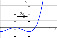
It should be possible to avoid higher excitations in the symmetry-broken phase , thus mitigating the effects of the cut-off, by changing the basis such that the operator in the new basis has an expectation value of approximately zero . We effectively shift the origin in a plot of the effective potential by some amount towards the minimum, such that fluctuations are centered about . That higher excitations in the shifted number basis are then avoided seems intuitively reasonable given the classical effective potential, where each of the two wells (in the symmetry-broken case) looks locally similar to a single-well potential. Figure 5 illustrates this procedure.
The change of basis corresponds to the unitary
with being the conjugate momentum operator of (35). It defines new creation and annihilation operators
such that where characterizes the shift. In terms of operators in the shifted basis, the Hamiltonian is
Using this Hamiltonian with a value of should thus help to avoid higher excitations and allow us to efficiently represent ground states with large values of .
III.1.3 Effects of the Hilbert space cut-off
The effects of the local Hilbert space cut-off are, as expected, relatively strong near to the critical point, becoming weaker further into the symmetry-broken phase when using the shifted basis (see Figure 6). Without the basis shift, states with large values of exhibit a weight-shift towards higher modes, as illustrated in Figure 7. In all cases, excitation of higher modes drops off exponentially, with being sufficient to capture the most significant contributions, as demonstrated in Figure 8.


The shifted basis has an added benefit when sweeping in the broken phase and using the previous ground state approximation as a starting state for the next ground-state search. In this case, adjusting the shift towards the next predicted (according to a preliminary fit of (37)) improves the starting state by bringing closer to the new ground-state value, leading to faster convergence. This is because a shift of always centers the state about the origin in the shifted basis (see Figure 9). Adjusting the shift by some also adjusts by the same amount.
III.1.4 Locating the critical point using the field expectation value
As noted in section I.4, since is the order-parameter associated with the -theory phase-change, it can be used to identify the critical point. A possible strategy for finding the critical parameters for might thus be to fix and sweep until one sees a transition from to or vice versa. However, this is not practical because the amount of entanglement in the ground state (for example, as quantified by the half-chain entropy (15)) tends to infinity as the critical point is approached, such that accurate representation using uMPS requires the bond-dimension to approach infinity also. Since the computational complexity of the TDVP algorithm scales as , this bisection method cannot achieve high accuracy for reasons of practicality.
Instead, we approach the critical point from the symmetry-broken phase, noting that physical quantities obey power laws in the vicinity of critical points (see section I.4). For we can thus write
| (37) |
where is a constant, is the critical exponent and is the critical value of for a given . Fitting this equation to as a function of (with fixed ) as near as possible to the phase-transition, we obtain an estimate for the lattice critical parameter . We can then use a series of fits with to extrapolate an estimate for the critical parameter of the continuum theory.
Initial simulations show that, as expected, the half-chain entropy of the ground state approximation tends to infinity as the critical point is approached. This is visible in Figure 10, where we show results obtained from high bond dimension limits as well as using a fixed bond-dimension. As further confirmed in Figures 11 and 12, a fixed is not sufficient to capture ground states near the critical point.


Note that a phase transition does, in fact, occur for fixed , albeit not at the exact critical point, but at increasingly lower values of for decreasing values of (and for decreasing ). This is consistent with the entropy shown in Figure 10, which is asymmetric about the critical point, falling off more slowly in the symmetric phase. Since a fixed represents an upper bound on the amount of entanglement in the state (see section II.1), the uMPS variational manifold comes closer to the exact ground-state when its entropy is lower. Given the asymmetric entropy of -theory, this implies that symmetry-broken ground-states are easier to approximate than symmetrical ones (for a given distance in parameter space from the critical point). For a symmetric ground state with high entropy, a low-lying excited state with much lower entropy may thus turn out to be the best available ground state approximation in . Such an excitation should be available for such states, since a small change in the parameter results in an asymmetric ground state (on the other side of the critical point). The situation is illustrated in Figure 13. The same -dependent shift of the critical point is observed with the transverse Ising model [35].

One might consider using this behavior together with finite-entanglement scaling techniques [35] to obtain information about the true critical point (for example, the critical exponent), but this requires precise knowledge of its location. Instead, we take data at several values of in order to obtain high- limits of , which we then fit using (37) to obtain an estimate for the location as well as the critical exponent.
Since we take a high- limit of the approximate ground-state value of for each parameter combination (requiring a higher for the higher-entropy states closer to the critical point) there is a practical limit on how near we can come. This is unfortunate, since the fit (37) is highly sensitive to near-critical points, where the gradient goes to infinity. Power-law scaling is also only exactly fulfilled infinitesimally close to the critical point, such that including data points further away decreases accuracy. We thus only fit the points closest to the critical point for which we have sufficient (in terms of bond-dimension) data.
III.1.5 Locating the critical point using excitations
Another approach to finding the critical parameters, given , is to plot the energy of the lowest-lying excitation against , which should tend to zero as we approach the critical point from either side. We describe an ansatz for obtaining the lowest-lying excitation energies, given a uMPS approximation to the ground state, in section II.3.
In obtaining excitation energies in the symmetry-broken phase, topologically non-trivial excitations must be taken into account. This precludes the use of the -shifted basis mentioned in section III.1.1 to represent the state, since approximations to both possible ground states are required for the calculations and these must use the same basis. For reasons of efficiency, it thus makes sense to focus on states near to the critical point where the shifted basis is not needed. This should not cause problems since this is where we expect power-law scaling to be more exactly fulfilled.
We first locate the lowest-lying excitation of the symmetry-broken phase and determine whether it is topologically trivial or non-trivial, whilst confirming that it goes to zero for some value of . To do this, we use the excitation ansatz to determine dispersion relations for the lowest-lying topologically trivial and non-trivial excitations for fixed and several values of . We then use linear extrapolation of the excitation energies at each momentum to obtain a dispersion relation at the first point where one of them goes to zero, which should correspond to the lattice critical point . The result is shown in Figure 14, where we see that the lowest-lying excitations are the topologically non-trivial soliton (kink) excitations (at zero momentum). A plot of this excitation energy versus exhibits almost exactly linear scaling, consistent with the transverse Ising model, suggesting the use of linear regression to obtain an estimate for the critical parameter. The plot is shown in Figure 15, which contains the excitation energies obtained for several bond-dimensions. The small change in excitation energy near the critical point when increasing the bond-dimension from to , compared with the change in shown in Figure 11 (for a larger lattice-spacing), suggests that finite-entanglement effects are less severe for the excitation energy than for . Certainly, the ground-state energy should reach a high- limit sooner than simply because the approximate ground state is close to the energy minimum. Also, if the exact lowest-lying excitation is highly localized, we should need only a relatively low to approximate it well. It seems excitations present a less computationally-intensive way of obtaining a good estimate for the critical parameter, compared with .


We note that, for fixed , the lowest-lying (soliton) excitation receives a negative energy (with respect to the approximate uniform ground-state) for sufficiently low values of (see Figure 15). The position of this crossover is very close to the critical point predicted by linear extrapolation. The existence of negative approximate excitation energies indicates that the topologically non-trivial ansatz states include a better approximation to the exact ground state than . This is consistent with the -dependent shift of the apparent phase-transition of : If the exact ground state is symmetric, but the approximate ground state is asymmetric, a topologically non-trivial excitation interpolating between the two degenerate asymmetric approximate ground states should be locally closer to the exact ground state at the disturbance.
In fact, we can construct a better uMPS ground-state approximation using negative-energy kink “excitations” by defining new parameter matrices
where and are the parameters for the two original ground states, and are the tangent-vector parameters for a kink and an anti-kink and . The resulting state contains the original ground states as well as kink states at order plus multi-kink states at . This leads to energy contributions (there are no kink contributions at order because the kinks are orthogonal to the original ground states). Since the state can, depending on , have a lower energy than . can be interpreted as a kink-density with an optimal value depending on the higher-order energy contributions.
III.1.6 Mean-field theory
When , the uMPS variational class is the same as that of the uniform product states (or mean field theory (MFT) states)
where and . In this case, the per-site energy expectation value takes on an effective one-particle form
where is the -variance . An approximation to the ground state can then be found by applying the time-independent variational principle and minimizing with respect to the parameters , which can be taken to be real since all matrix elements in the above expression are real. The gradient of is also readily obtainable
making many commonly-used minimizing algorithms applicable, such as the quasi-Newton method of Broyden, Fletcher, Goldfarb, and Shanno (BFGS) [36]. This method is much simpler and more efficient than applying the imaginary-time TDVP algorithm for uMPS with .
Normalization presents a minor complication. The above equations assume , which imposes a constraint on the variational parameters. Rather than using a constrained optimizer, we eliminate the norm degree of freedom by switching to -dimensional spherical coordinates such that the norm corresponds to a single parameter and can easily be fixed and ignored.
To estimate the location of the lattice critical point using MFT, we again obtain ground states for a sweep of for some fixed . As in the more general case of uMPS with fixed , we are putting a restriction on entanglement by using MFT () and thus expect an apparent phase-transition to occur at some value of for a given . We use the location of the apparent transition as an estimate for , obtaining it from both and excitation energies calculated using the MFT excitation ansatz of section II.3.1. Since we do not expect power-law scaling of physical quantities to be reproduced by MFT, we do not attempt to fit data using power laws. Instead, we use bisection to pin down the apparent phase-transition in , which is possible due to the relative ease of finding MFT ground states, and interpolate the lowest-lying excitation energies (in the apparently symmetry-broken phase) to obtain the point at which they become negative (these excitations are topologically non-trivial, as for — see the above explanation).
Although we can obtain estimates for the lattice critical point using these methods, we do not expect to obtain useful information about the continuum critical theory due to the lack of entanglement. However, since it is also possible to interpret the lattice critical point as a continuum limit of a non-critical theory (see section I.4), an ability to estimate its location using mean-field theory indicates that useful predictions about non-critical continuum theories can be made.
III.1.7 Central charge
We determine the central charge associated with the conformal field theory of the critical system using finite-entanglement scaling techniques. It is known that, for infinite one-dimensional systems with a second-order phase-transition, the half-chain entropy of the ground state in the vicinity of a critical point with conformal invariance is
| (38) |
where is the correlation length and is the “central charge” [33]. Approaching the critical point, and the entropy diverges. The central charge specifies a conformal field theory (CFT), which describes behavior at the critical point in the continuum limit.
We know from (15) that the maximum half-chain entropy of a uMPS state, contained, assuming right canonical form, in the diagonal entries of the matrix , is directly related to the bond-dimension , which is also the maximum Schmidt-rank of the corresponding Schmidt decomposition. Thus, for lower values of , finite-entanglement effects occur and the value of scales with . It turns out there is a simple relationship between , , and describing this scaling [31]
| (39) |
We can thus obtain an estimate for from values of taken from a number of ground state approximations with varying . For this to work, we must be close enough to the critical point so that (38) is valid and use small enough so that is limited by finite-entanglement effects. We can then use linear regression to fit (39) and obtain .
III.2 Results and analysis
III.2.1 Estimates of the continuum critical parameter
Figure 16 shows estimates for the critical parameter taken from sweep plots of and of the lowest-lying excitation energy , approaching the continuum limit .


| Fit function | dof | dof | ||
|---|---|---|---|---|
| 65.10(18) | 65.22(24) | 676 | ||
| 65.61(16) | 65.79(17) | 186 | ||
| 66.01(11) | 771 | 66.19(11) | 44.8 | |
| 66.30(2) | 19.7 | 66.46(5) | 4.67 | |
| 66.26(3) | 24.8 | 66.42(5) | 6.22 | |
The two sets of values show good agreement, with the largest discrepancy occurring for , where we found high- limits of particularly close to the critical point without resorting to very high bond-dimensions. Excluding the points of lowest from the fit pushes the fitted value of upwards, closer to the value, leading us to speculate that the excluded values were not accurate enough, possibly due to insufficient convergence of the uMPS ground state. We are inclined to trust the results obtained from the data over those from fits to , in particular due to the relative robustness of the linear regression fit to errors made near the critical point.
As expected (see section I.4), non-linear behavior of is present. Given that the exact behavior is unknown, but is predicted to be logarithmic, we follow [21] and fit a series of functions, evaluating the statistic to judge which can be reasonably used to predict a continuum value . The results of the fits are listed in Table 1, where we define our final estimates for to be the fitted values with reduced statistic dof closest to one.
We find that the critical exponent obtained only from fits to agrees poorly with the predicted transverse Ising value of , the fitted values near the continuum limit being significantly higher, as shown in Figure 16. This we attribute to insufficient data near to the lattice critical points, noting that the effect of excluding the points of lowest is to increase the fitted value of further. Using the values taken from the data together with the data, we obtain a second estimate of that, in the continuum limit , shows a much clearer trend towards the Ising value, in support of the greater reliability of the -based estimates of the critical parameter.

III.2.2 Mean-field results
Due to the lack of entanglement in the mean-field class (see section III.1.4), we expect a large shift of the apparent phase-transition to lower values of . We observe that the shift takes the apparent phase-transition (in and in ) towards in the continuum limit (see Figure 17). For higher values of , the apparent phase-transition starts to approach the approximate critical parameters obtained above using uMPS with . The mean-field excitations data gives better predictions for the critical parameters than , in agreement with the relatively low sensitivity of the excitation energies to the bond-dimension observed with uMPS.
III.2.3 Central charge
We extract the central charge by finding approximate uMPS ground states for various low bond-dimensions at (or very near) the lattice critical point as determined from the uMPS excitations data. We observe approximately linear scaling of the entropy, as predicted by (39), with the central charge extracted from the gradient of a linear fit agreeing well, for larger values of , with the prediction of from the transverse Ising model. For lower values of , we find that the gradient often agrees poorly with , despite the scaling remaining linear. At this point, we do not have a good explanation for this discrepancy, so we leave it as a subject for future investigations. Our results are summarized in Figure 18.


III.2.4 Spectral density
To further demonstrate the convenience of having approximate ground states in uMPS form and the usefulness of the uMPS excitation ansatz, we obtain the spectral density function (4) from the overlap of approximate excited states with the approximate uMPS ground state. Results for states in the symmetry-broken and in the symmetric phase are shown in Figure 19 and Figure 20 respectively. By interpreting the lattice critical point as a continuum limit of a non-critical theory (see section I.4), a series of such plots could be used to extrapolate a continuum spectral density for that theory. The nature of the uMPS excitation ansatz means that not all excitations can be captured. This explains the lack of a continuum of excitations, expected soon after the single-particle state. It would be interesting to compare the results with those of other approaches such as [37].


III.3 Discussion
The consistency of the lattice critical parameters obtained from approximate uMPS ground-state field expectation values and those derived from the lowest-level excitation energies calculated using the uMPS excitation ansatz, as well as agreement of the critical exponents with their transverse Ising counterparts, demonstrates the validity of both methods for studying critical -dimensional -theory. The finite-entanglement scaling method we use to obtain estimates for the central charge of critical -theory shows promise: Approximate linear scaling of the entropy with is observed, as predicted, and the fitted values for agree with the transverse Ising value for higher values of . However, further work is needed to explain the discrepancies observed for lower .
We find uMPS to be an excellent class of ansatz states for studying the critical phenomena of -dimensional -theory due to the amount of entanglement in near-critical ground states being the main barrier to their efficient representation. With MPS, the amount of entanglement that can be represented is controllable via the bond-dimension , which can easily be varied to obtain the limiting behavior of quantities such as . In this way, we can avoid errors originating from finite-entanglement effects. Additionally, working directly in the thermodynamic limit of an infinite lattice completely avoids additional finite-size effects and the need for further scaling investigations. Obtaining ground states using our variational conjugate gradient method (or the TDVP with imaginary time evolution) is also very convenient, since we need only enough storage capacity to capture the approximate state at one point in time, unlike when simulating the Euclidean theory on a space-time lattice. Also, using the TDVP, the computational complexity scales linearly in .
The class of uniform mean-field states (uMPS with ), despite featuring no entanglement, appears suited to estimating properties of non-critical continuum theories in some cases, even if not of critical theories. Owing to the relative ease with which MFT ground-state approximations and excitation energies can be obtained, and the low computational cost of extending them to higher space-time dimensions (due to the lack of entanglement), these methods represent another useful tool for investigating quantum field theories.
III.3.1 Comparison to other methods
We summarize existing literature estimates for the continuum critical parameter in Table 2, where we include our results from Table 1 with dof values closest to one. Our estimates agree poorly with the DMRG result of [18], but relatively well with the Monte Carlo results of [21]. With regard to the DMRG results, where the technique used is similar to ours, we can attribute the large difference to finite-entanglement effects, since these serve to shift the apparent critical point to lower values of , with a larger shift for smaller lattice-spacings. The DMRG parameters used in [18] correspond to [38], resulting in a relatively large shift (see Figure 11). The DMRG study also uses only two lattice critical points to extrapolate a continuum value and, as such, misses the non-linear behavior of . The Monte Carlo methods used in [21] are very different to ours. They work with the Euclidean theory on a finite two-dimensional lattice whereas we work on an infinite spatial lattice in continuous time (numerical integration of the TDVP flow equations could be seen as analogous to discretizing imaginary time on a lattice, in which case our temporal “lattice” is of the length necessary to produce sufficient convergence of the approximate ground-state). Rather than taking finite-size scaling limits, we take finite-entanglement scaling limits to obtain our ground-state approximations. Noting these differences, the fact that our results agree to within gives us confidence in the methods used.
| Method | Reference | |
| uMPS, TDVP, | 66.46(5) | This work |
| uMPS, TDVP, | 66.30(2) | This work |
| Monte Carlo | [21] | |
| Gaussian effective potential | 61.632 | [39] |
| Gaussian effective potential | 61.266 | [16] |
| GEP and oscillator rep. | 61.26 | [40] |
| Spherical field theory | 60.3 | [41] |
| Diffusion Monte Carlo | [42] | |
| DMRG | 59.89(1) | [18] |
| Continuum light-front | 59.46 | [43] |
| Connected Green function | 58.70 | [39] |
| Coupled cluster expansion | [44] | |
| Discretized light-front | 43.95, 46.26 | [45] |
| Discretized light-front | 43.70, 33.00 | [46, 47] |
| Random phase approximation | 43.2 | [48] |
| Non-Gaussian variational | 41.28 | [49] |
Conclusion
The class of uniform matrix product states (uMPS) appears well-suited to the study of critical quantum fields in dimensions via lattice regularization. Using variational methods like our naive variational conjugate gradient method or the imaginary-time time-dependent variational principle (TDVP) (where the former provides significantly improved convergence speed for the system studied), good approximations to ground states can be obtained efficiently, even near to the critical point. Here, the correspondence between the bond dimension and the maximum entanglement of a state allows the use of finite-entanglement scaling to judge the accuracy of physical quantities calculated. Compared to Monte Carlo simulations, uMPS allows us to work directly in the thermodynamic limit and has storage requirements independent of the imaginary time dimension. Further, low-lying excitation energies are straightforward to calculate, enabling the study of dispersion relations and the spectral density. Even mean field theory shows potential for delivering useful predictions about non-critical continuum theories.
Acknowledgments — Helpful discussions with Florian Richter and Cédric Bény are gratefully acknowledged. This work was supported by the ERC grant QFTCMPS and by the cluster of excellence EXC 201 Quantum Engineering and Space-Time Research.
Appendix A Minimization using conjugate-gradient methods

When minimizing functions that are approximately quadratic in their parameters, which is always true in the vicinity of a minimum (assuming sufficient differentiability), making steps along the gradient direction (gradient-descent) is often a sub-optimal way of reaching the minimum.
We can illustrate this using a quadratic function of two variables as shown in the figure to the right. Beginning at some point near the minimum and using a line-search to find the minimum of in that direction to determine each step size (green line), an unfortunate starting position can result in a long zig-zag path and a large number of steps.
To avoid this, we can use the conjugate-gradient method [36], which works by only stepping in directions that are conjugate to those already used. Writing a general quadratic function of many variables as
with , , we can define and such that:
A vector is conjugate to another vector with respect to if and only if . The gradient of the function is
such that a stationary point satisfies . Given a basis consisting of mutually conjugate vectors , we can expand in that basis with coefficients dependent only on the corresponding basis vectors:
This means we can pick a starting vector and proceed to the minimum in exactly steps by finding successive that are conjugate to all previous , where the step-size is uniquely determined by the current direction . This can be further improved on by choosing specific
where is the negative gradient and is a number defined below. We make steps
with
where . Requiring and then result in
so that we only need to know and to calculate the next step. The red line in the above illustration demonstrates this procedure. We can modify this version of the conjugate-gradient method again so that it can iteratively find the solution of approximately quadratic problems. In this case, we must treat the function and its gradient as black boxes. We can do this by obtaining an approximate , which is the only quantity requiring direct knowledge of , by doing a line-search to find the minimum of . The algorithm, known as the non-linear conjugate gradient method, is then:
- 1.
Calculate .
- 2.
Compute .
- 3.
Calculate the next conjugate vector .
- 4.
Use a line-search to find .
- 5.
Set new position .
The initial values are . If is exactly quadratic and we ignore all numerical error, this algorithm will find the minimum in iterations or less. With an approximately quadratic and/or accounting for limited numerical precision, the vectors will not be exactly conjugate to each other and errors will accumulate. The algorithm must therefore be re-started at least every iterations. Note that there are other choices for that are equivalent in the quadratic case, but result in different non-linear conjugate gradient algorithms. The above choice is the one originally used by Fletcher and Reeves [51].
Appendix B Matrix elements for phi-4-theory
The matrix elements of the operators needed to implement the -theory Hamiltonian using the site number-basis defined in section III are as follows:
References
- [1] M. E. Peskin and D. V. Schroeder, An Introduction To Quantum Field Theory (Westview Press, 1995).
- [2] ATLAS-Collaboration, Phys Lett B 716, 1 (2012).
- [3] M. Creutz, Quarks, Gluons and Lattices (Cambridge University Press, 1985).
- [4] W. von der Linden, Phys. Rep. 220, 53 (1992).
- [5] S. Dürr, Z. Fodor, J. Frison, C. Hoelbling, R. Hoffmann, S. D. Katz, S. Krieg, T. Kurth, L. Lellouch, T. Lippert, K. K. Szabo, and G. Vulvert, Int S Techn Pol Inn 322, 1224 (2008).
- [6] S. R. White, Phys Rev Lett 69, 2863 (1992).
- [7] U. Schollwöck, Rev Mod Phys 77, 259 (2005).
- [8] J. Eisert, M. Cramer, and M. B. Plenio, Rev Mod Phys 82, 277 (2010).
- [9] M. B. Hastings, J Stat Mech-Theory E 2007, P08024 (2007).
- [10] T. J. Osborne, Phys Rev Lett 97, 157202 (2006a).
- [11] N. de Beaudrap, M. Ohliger, T. J. Osborne, and J. Eisert, Phys Rev Lett 105, 060504 (2010).
- [12] M. B. Hastings, Phys Rev B 73, 085115 (2006).
- [13] L. Masanes, Phys Rev A 80, 052104 (2009).
- [14] J. Haegeman, J. I. Cirac, T. J. Osborne, I. Pižorn, H. Verschelde, and F. Verstraete, Phys Rev Lett 107, 070601 (2011).
- [15] J. Haegeman, B. Pirvu, D. J. Weir, J. I. Cirac, T. J. Osborne, H. Verschelde, and F. Verstraete, Phys Rev B 85, 100408 (2012a).
- [16] S.-J. Chang, Phys Rev D 13, 2778 (1976).
- [17] B. Simon and R. B. Griffiths, Commun Math Phys 33, 145–164 (1973).
- [18] T. Sugihara, J High Energy Phys 2004, 007 (2004).
- [19] D. J. Weir, Phys Rev D 82, 025003 (2010).
- [20] W. Loinaz and R. S. Willey, Phys Rev D 58, 076003 (1998).
- [21] D. Schaich and W. Loinaz, Phys Rev D 79, 056008 (2009).
- [22] A. K. De, A. Harindranath, J. Maiti, and T. Sinha, Phys Rev D 72, 094503 (2005).
- [23] A. Milsted, “evoMPS,” GitHub (BSD License).
- [24] D. C. Brydges, J. Fröhlich, and A. D. Sokal, Commun Math Phys 91, 141 (1983).
- [25] S. P. Jordan, K. S. M. Lee, and J. Preskill, arXiv (2011), 1112.4833 .
- [26] R. Jackiw and S. Templeton, Phys Rev D 23, 2291 (1981).
- [27] S. Sachdev, Quantum Phase Transitions, 2nd ed. (Cambridge University Press, 2011).
- [28] H. Kleinert and V. Schulte-Frohlinde, Critical Properties of Phi-4-theories (World Scientific Publishing Co Pte Ltd, 2001).
- [29] J. Haegeman, M. Mariën, T. J. Osborne, and F. Verstraete, arXiv (2012b), 1210.7710 .
- [30] P.-A. Absil, R. Mahony, and R. Sepulchre, Optimization Algorithms on Matrix Manifolds (Princeton University Press, 2009).
- [31] F. Pollmann, S. Mukerjee, A. M. Turner, and J. E. Moore, Phys Rev Lett 102, 255701 (2009).
- [32] J. I. Latorre, E. Rico, and G. Vidal, arXiv (2003), Quant Inf Comput 4 (2004) 48-92, quant-ph/0304098 .
- [33] P. Calabrese and J. Cardy, J Stat Mech-Theory E 2004, P06002 (2004).
- [34] G. Vidal, J. I. Latorre, E. Rico, and A. Kitaev, Phys Rev Lett 90, 227902 (2003).
- [35] L. Tagliacozzo, T. R. de Oliveira, S. Iblisdir, and J. I. Latorre, Phys Rev B 78, 024410 (2008).
- [36] W. Press, S. Teukolsky, W. Vetterling, and B. Flannery, Numerical Recipes: The Art of Scientific Computing, 3rd ed. (Cambridge University Press, New York, 2007).
- [37] T. J. Osborne, arXiv (2006b), cond-mat/0605194 .
- [38] S. Rommer and S. Östlund, Phys Rev B 55, 2164 (1997).
- [39] J. M. Häuser, W. Cassing, A. Peter, and M. H. Thoma, Z Phys A-Hadron Nuc 353, 301 (1995).
- [40] C.-R. Ji, J.-I. Kim, D.-P. Min, and A. V. Vinnikov, arXiv (2002), hep-ph/0204114 .
- [41] D. Lee, Phys Lett B 439, 85 (1998).
- [42] P. J. Marrero, E. A. Roura, and D. Lee, Phys Lett B 471, 45 (1999).
- [43] C. M. Bender, S. Pinsky, and B. van de Sande, Phys Rev D 48, 816 (1993).
- [44] M. Funke, U. Kaulfuss, and H. Kümmel, Phys Rev D 35, 621 (1987).
- [45] T. Sugihara, Phys Rev D 57, 7373 (1998).
- [46] A. Harindranath and J. P. Vary, Phys Rev D 36, 1141 (1987).
- [47] A. Harindranath and J. P. Vary, Phys Rev D 37, 1076 (1988).
- [48] H. Hansen, G. Chanfray, D. Davesne, and P. Schuck, Eur Phys J A 14, 397 (2002).
- [49] L. Polley and U. Ritschel, Phys Lett B 221, 44 (1989).
- [50] O. Alexandrov, “Conjugate gradient illustration (public domain),” (2007).
- [51] R. Fletcher and C. M. Reeves, Comput. J 7, 149 (1964).
