Nonparametric Basis Pursuit
via Sparse Kernel-based Learning†
Abstract
Signal processing tasks as fundamental as sampling, reconstruction, minimum mean-square error interpolation and prediction can be viewed under the prism of reproducing kernel Hilbert spaces. Endowing this vantage point with contemporary advances in sparsity-aware modeling and processing, promotes the nonparametric basis pursuit advocated in this paper as the overarching framework for the confluence of kernel-based learning (KBL) approaches leveraging sparse linear regression, nuclear-norm regularization, and dictionary learning. The novel sparse KBL toolbox goes beyond translating sparse parametric approaches to their nonparametric counterparts, to incorporate new possibilities such as multi-kernel selection and matrix smoothing. The impact of sparse KBL to signal processing applications is illustrated through test cases from cognitive radio sensing, microarray data imputation, and network traffic prediction.
I Introduction
Reproducing kernel Hilbert spaces (RKHSs) provide an orderly analytical framework for nonparametric regression, with the optimal kernel-based function estimate emerging as the solution of a regularized variational problem [33]. The pivotal role of RKHS is further appreciated through its connections to “workhorse” signal processing tasks, such as the Nyquist-Shannon sampling and reconstruction result that involves sinc kernels [24]. Alternatively, spline kernels replace sinc kernels, when smoothness rather than bandlimitedness is to be present in the underlying function space [31].
Kernel-based function estimation can be also seen from a Bayesian viewpoint. RKHS and linear minimum mean-square error (LMMSE) function estimators coincide when the pertinent covariance matrix equals the kernel Gram matrix. This equivalence has been leveraged in the context of field estimation, where spatial LMMSE estimation referred to as Kriging, is tantamount to two-dimensional RKHS interpolation [10]. Finally, RKHS based function estimators can linked with Gaussian processes (GPs) obtained upon defining their covariances via kernels [25].
Yet another seemingly unrelated, but increasingly popular theme in contemporary statistical learning and signal processing, is that of matrix completion [12], where data organized in a matrix can have missing entries due to e.g., limitations in the acquisition process. This article builds on the assertion that imputing missing entries amounts to interpolation, as in classical sampling theory, but with the low-rank constraint replacing that of bandlimitedness. From this point of view, RKHS interpolation emerges as the prudent framework for matrix completion that allows effective incorporation of a priori information via kernels [3], including sparsity attributes.
Recent advances in sparse signal recovery and regression motivate a sparse kernel-based learning (KBL) redux, which is the purpose and core of the present paper. Building blocks of sparse signal processing include the (group) least-absolute shrinkage and selection operator (Lasso) and its weighted versions [16], compressive sampling [8], and nuclear norm regularization [12]. The common denominator behind these operators is the sparsity on a signal’s support that the -norm regularizer induces. Exploiting sparsity for KBL leads to several innovations regarding the selection of multiple kernels [23, 19], additive modeling [26, 21], collaborative filtering [3], matrix and tensor completion via dictionary learning [7], as well as nonparametric basis selection [6]. In this context, the main contribution of this paper is a nonparametric basis pursuit (NBP) tool, unifying and advancing a number of sparse KBL approaches.
Constrained by space limitations, a sample of applications stemming from such an encompassing analytical tool will be also delineated. Sparse KBL and its various forms contribute to computer vision [28, 32], cognitive radio sensing [6], management of user preferences [3], bioinformatics [29], econometrics [21, 26], and forecasting of electric prices, load, and renewables (e.g., wind speed) [18], to name a few.
The remainder of the paper is organized as follows. Section II reviews the theory of RKHS in connection with GPs, describing the Representer Theorem and the kernel trick, and presenting the Nyquist-Shannon Theorem (NST) as an example of KBL. Section III deals with sparse KBL including sparse additive models (SpAMs) and multiple kernel learning (MKL) as examples of additive nonparametric models. NBP is introduced in Section IV, with a basis expansion model capturing the general framework for sparse KBL. Blind versions of NBP for matrix completion and dictionary learning are developed in Sections V and VI. Finally, Section VII presents numerical tests using real and simulated data, including RF spectrum measurements, expression levels in yeast, and network traffic loads. Conclusions are drawn in Section VIII, while most technical details are deferred to the Appendix.
II KBL Preliminaries
In this section, basic tools and approaches are reviewed to place known schemes for nonparametric (function) estimation under a common denominator.
II-A RKHS and the Representer Theorem
In the context of reproducing kernel Hilbert spaces (RKHS) [33], nonparametric estimation of a function defined over a measurable space is performed via interpolation of training points where and . For this purpose, a kernel function selected to be symmetric and positive definite, specifies a linear space of interpolating functions given by
For many choices of , is exhaustive with respect to (w.r.t) families of functions obeying certain regularity conditions. The spline kernel for example, generates the Sobolev space of all low-curvature functions [11]. Likewise, the sinc kernel gives rise to the space of bandlimited functions. Space becomes a Hilbert space when equipped with the inner product , and the associated norm is . A key result in this context is the so-termed Representer Theorem [33], which asserts that based on , the optimal interpolator in , in the sense of
| (1) |
admits the finite-dimensional representation
| (2) |
This result is nice in its simplicity, since functions in space are compound by a numerable but arbitrarily large number of kernels, while is a combination of just a finite number of kernels around the training points. In addition, the regularizing term controls smoothness, and thus reduces overfitting. After substituting (2) into (1), the coefficients minimizing the regularized least-squares (LS) cost in (1) are given by , upon recognizing that , and defining as well as the kernel dependent Gram matrix with entries ( stands for transposition).
Remark 1. The finite-dimensional expansion (2) solves (1) for more general fitting costs and regularizing terms. In its general form, the Representer Theorem asserts that (2) is the solution
| (3) |
where the loss function replacing the LS cost in (1) can be selected to serve either robustness (e.g., using the absolute-value instead of the square error); or, application dependent objectives (e.g., the Hinge loss to serve classification applications); or, for accommodating non-Gaussian noise models when viewing (3) from a Bayesian angle. On the other hand, the regularization term can be chosen as any increasing function of the norm which will turn out to be crucial for introducing the notion of sparsity, as described in the ensuing sections.
II-B LMMSE, Kriging, and GPs
Instead of the deterministic treatment of the previous subsection, the unknown can be considered as a random process. The KBL estimate (2) offered by the Representer Theorem has been linked with the LMMSE-based estimator of random fields , under the term Kriging [10]. To predict the value at an exploration point via Kriging, the predictor is modeled as a linear combination of noisy samples at measurement points ; that is,
| (4) |
where are the expansion coefficients, and collects the data. The MSE criterion is adopted to find the optimal . Solving the latter yields , where and . If is zero-mean white noise with power , then and can be expressed in terms of the unobserved as , where , and , with . Hence, the LMMSE estimate in (4) takes the form
| (5) |
where and the -th entry of , denoted by , is indeed a function of the exploration point , and the measurement point .
With the Kriging estimate given by (5), the RKHS and LMMSE estimates coincide when the kernel in (2) is chosen equal to the covariance function in (5).
The linearity assumption in (4) is unnecessary when and are modeled as zero-mean GPs [25]. GPs are those in which instances of the field at arbitrary points are jointly Gaussian. Zero-mean GPs are specified by , which determines the covariance matrix of any vector comprising instances of the field, and thus its specific zero-mean Gaussian distribution. In particular, the vector collecting the field at the exploration and measurement points is Gaussian, and so is the vector Hence, the MMSE estimator, given by the expectation of conditioned on , reduces to [17]
| (6) |
II-C The kernel trick
Analogous to the spectral decomposition of matrices, Mercer’s Theorem establishes that if the symmetric positive definite kernel is square-integrable, it admits a possibly infinite eigenfunction decomposition [33], with where stands for Kronecker’s delta. Using the weighted eigenfunctions a point can be mapped to a vector (sequence) such that This mapping interprets a kernel as an inner product in , since for two points . Such an inner product interpretation forms the basis for the “kernel trick.”
The kernel trick allows for approaches that depend on inner products of functions (given by infinite kernel expansions) to be recast and implemented using finite dimensional covariance (kernel) matrices. A simple demonstration of this valuable property can be provided through kernel-based ridge regression. Starting from the standard ridge estimator for , and , it is possible to rewrite and solve . After is obtained in the training phase, it can be used for prediction of an ensuing given . By using the matrix inversion lemma, can be written as .
Now, if with is constructed from using eigenfunctions , then and , which yields
| (7) |
Expressing a linear predictor in terms of inner products only is instrumental for mapping it into its kernel-based version. Although the mapping entails the eigenfunctions , these are not explicitly present in (7), which is given solely in terms of . This is crucial since can be infinite dimensional which would render the method computationally intractable, and more importantly the explicit form of may not be available. Use of kernel trick was demonstrated in the context of ridge regression. However, the trick can be used in any vectorial regression or classification method whose result can be expressed in terms of inner products only. One such example is offered by support vector machines, which find a kernel-based version of the optimal linear classifier in the sense of minimizing Vapnik’s -insensitive Hinge loss function, and can be shown equivalent to the Lasso [14].
In a nutshell, the kernel trick provides a means of designing KBL algorithms, both for nonparametric function estimation [cf. (1)], as well as for classification.
II-D KBL vis à vis Nyquist-Shannon Theorem
Kernels can be clearly viewed as interpolating bases [cf. (2)]. This viewpoint can be further appreciated if one considers the family of bandlimited functions , where denotes the class of square-integrable functions defined over (e.g., continuous-time, finite-power signals). The family constitutes a linear space. Moreover, any can be generated as the linear combination (span) of sinc functions; that is, . This is the cornerstone of signal processing, namely the NST for sampling and reconstruction, but can be viewed also under the lens of RKHS with as a reproducing kernel [24]. The following properties (which are proved in the Appendix) elaborate further on this connection.
P1. The sinc-kernel Gram matrix satisfies .
P2. The sinc kernel decomposes over orthonormal eigenfunctions .
P3. The RKHS norm is .
P1 states that qualifies as a kernel, while P2 characterizes the eigenfunctions used in the kernel trick, and P3 shows that the RKHS norm is the restriction of the norm to .
P1-P3 establish that the space of bandlimited functions is indeed an RKHS. Any can thus be decomposed as a numerable combination of eigenfunctions, where the coefficients and eigenfunctions obey the NST. Consequently, existence of eigenfunctions spanning is a direct consequence of being a RKHS, and does not require the NST unless an explicit form for is desired. Finally, strict adherence to NST requires an infinite number of samples to reconstruct . Alternatively, the Representer Theorem fits to a finite set of (possibly noisy) samples by regularizing the power of .
III Sparse additive nonparametric modeling
The account of sparse KBL methods begins with SpAMs and MKL approaches. Both model the function to be learned as a sparse sum of nonparametric components, and both rely on group Lasso to find it. The additive models considered in this section will naturally lend themselves to the general model for NBP introduced in Section IV, and used henceforth.
III-A SpAMs for High-Dimensional Models
Additive function models offer a generalization of linear regression to the nonparametric setup, on the premise of dealing with the curse of dimensionality, which is inherent to learning from high dimensional data [16].
Consider learning a multivariate function defined over the Cartesian product of measurable spaces . Let denote a point in , the kernel defined over , and its associated RKHS. Although can be interpolated from data via (1) after substituting for , the fidelity of (2) is severely degraded in high dimensions. Indeed, the accuracy of (2) depends on the availability of nearby points , where the function is fit to the (possibly noisy) data . But proximity of points in high dimensions is challenged by the curse of dimensionality, demanding an excessively large dataset. For instance, consider positioning datapoints randomly in the hypercube , repeatedly for growing unbounded and constant. Then ; that is, the expected distance between any two points is equal to the side of the hypercube [16].
To overcome this problem, an additional modeling assumption is well motivated, namely constraining to the family of separable functions of the form
| (8) |
with depending only on the -th entry of , as in e.g., linear regression models . With separable as in (8), the interpolation task is split into one-dimensional problems that are not affected by the curse of dimensionality.
The additive form in (8) is also amenable to subsect selection, which yields a SpAM. As in sparse linear regression, SpAMs involve functions in (8) that can be expressed using only a few entries of . Those can be learned using a variational version of the Lasso given by [26]
| (9) |
where .
With denoting the th entry of , the Representer Theorem (3) can be applied per component in (9), yielding kernel expansions with scalar coefficients . The fact that (9) yields a SpAM is demonstrated by substituting these expansions back into (9) and solving for , to obtain
| (10) |
where is the Gram matrix associated with kernel , and denotes the weighted -norm .
III-B Nonparametric Lasso
Problem (10) constitutes a weighted version of the group Lasso formulation for sparse linear regression. Its solution can be found either via block coordinate descent (BCD) [26], or by substituting and applying the alternating-direction method of multipliers (ADMM) [6], with convergence guaranteed by its convexity and the separable structure of the its non-differentiable term [30]. In any case, group Lasso regularizes sub-vectors separately, effecting group-sparsity in the estimates; that is, some of the vectors in (10) end up being identically zero. To gain intuition on this, (10) can be rewritten using the change of variables , with and . It will be argued that if exceeds a threshold, then the optimal and thus will be null. Focusing on the minimization of (10) w.r.t. a particular sub-vector , as in a BCD algorithm, the substitute variables and should minimize
| (11) |
where Minimizing (11) over is a convex univariate problem whose solution lies either at the border of the constraint, or, at a stationary point; that is,
| (12) |
The Cauchy-Schwarz inequality implies that holds for any with . Hence, it follows from (12) that if , then , and thus .
The sparsifying effect of (9) on the additive model (8) is now revealed. If is selected large enough, some of the optimal sub-vectors will be null, and the corresponding functions will be identically zero in (8). Thus, estimation via (9) provides a nonparametric counterpart of Lasso, offering the flexibility of selecting the most informative component-function regressors in the additive model.
The separable structure postulated in (8) facilitates subset selection in the nonparametric setup, and mitigates the problem of interpolating scattered data in high dimensions. However, such a model reduction may render (8) inaccurate, in which case extra components depending on two or more variables can be added, turning (8) into the ANOVA model [21].
III-C Multi-Kernel Learning
Specifying the kernel that “shapes” , and thus judiciously determines in (1) is a prerequisite for KBL. Different candidate kernels would produce different function estimates. Convex combinations can be also employed in (1), since elements of the convex hull conserve the defining properties of kernels.
A data-driven strategy to select “the best” is to incorporate the kernel as a variable in (3), that is [19]
| (13) |
where the notation emphasizes dependence on .
Then, the following Lemma brings MKL to the ambit of sparse additive nonparametric models.
Lemma 1 ([23])
Let be a set of kernels and an element of their convex hull . Denote by and the RKHSs corresponding to and , respectively, and by the direct sum It then holds that:
- a)
; and
- b)
.
MKL as in (14) resembles (9), differing in that components in (14) depend on the same variable . Taking into account this difference, (14) is reducible to (10) and thus solvable via BCD or ADMoM, after substituting for . On the other hand, a more general case of MKL is presented in [23], where is the convex hull of an infinite and possibly uncountable family of kernels.
An example of MKL applied to wireless communications is offered in Section VII, where two different kernels are employed for estimating path-loss and shadowing propagation effects in a cognitive radio sensing paradigm.
In the ensuing section, basis functions depending on a second variable will be incorporated to broaden the scope of the additive models just described.
IV Nonparametric basis pursuit
Consider function over the Cartesian product of spaces and with associated RKHSs and , respectively. Let abide to the bilinear expansion form
| (15) |
where can be viewed as bases, and as expansion coefficient functions. Given a finite number of training data, learning under sparsity constraints constitutes the goal of the NBP approaches developed in the following sections.
The first method for sparse KBL of in (15) is related to a nonparametric counterpart of basis pursuit, with the goal of fitting the function to data, where are prescribed and s are to be learned. The designer’s degree of confidence on the modeling assumptions is key to deciding whether s should be prescribed or learned from data. If the prescribed s are unreliable, model (15) will be inaccurate and the performance of KBL will suffer. But neglecting the prior knowledge conveyed by s may be also damaging. Parametric basis pursuit [9] hints toward addressing this tradeoff by offering a compromising alternative.
A functional dependence between input and output is modeled in [9] with an overcomplete set of bases (a.k.a. regressors) as
| (16) |
Certainly, leveraging an overcomplete set of bases can accommodate uncertainty. Practical merits of basis pursuit however, hinge on its capability to learn the few s that “best” explain the given data.
The crux of NBP on the other hand, is to fit with a basis expansion over the domain, but learn its dependence on through nonparametric means. Model (15) comes handy for this purpose, when is a generally overcomplete collection of prescribed bases.
With known, need to be estimated, and a kernel-based strategy can be adopted to this end. Accordingly, the optimal function is searched over the family , which constitutes the feasible set for the NBP-tailored nonparametric Lasso [cf. (9)]
| (17) |
The Representer Theorem in its general form (3) can be applied recursively to minimize (17) w.r.t. each at a time, rendering expressible in terms of the kernel expansion as , where coefficients are learned from data via group Lasso [cf. (10)]
| (18) |
with .
As it was argued in Section III, group Lasso in (18) effects group-sparsity in the subvectors . This property inherited by (17) is the capability of selecting bases in the nonparametric setup. Indeed, by zeroing the corresponding coefficient function is driven to zero, and correspondingly drops from the expansion (15).
Remark 2. A single kernel and associated RKHS can be used for all components in (17), since the summands in (15) are differentiated through the bases. Specifically, for a common , a different per coefficient , yields a distinct diagonal matrix , defining an individual in (18) that renders vector identifiable. This is a particular characteristic of (17), in contrast with (9) and Lemma 1 which are designed for, and require, multiple kernels.
Remark 3. The different sparse kernel-based approaches presented so far, namely SpAMs, MKL, and NBP, should not be viewed as competing but rather as complementary choices. Multiple kernels can be used in basis pursuit, and a separable model for may be due in high dimensions. An NBP-MKL hybrid applied to spectrum cartography illustrates this point in Section VII, where bases are utilized for the frequency domain .
V Blind NBP for matrix and tensor completion
A kernel-based matrix completion scheme will be developed in this section using a blind version of NBP, in which bases will not be prescribed, but they will be learned together with coefficient functions . The matrix completion task entails imputation of missing entries of a data matrix . Entries of an index matrix specify whether datum is available (), or missing (). Low rank of is a popular attribute that relates missing with available data, thus granting feasibility to the imputation task. Low-rank matrix imputation is achieved by solving
| (19) |
where stands for the Hadamard (element-wise) product. The low-rank constraint corresponds to an upperbound on the number of nonzero singular values of matrix , as given by its -norm. Specifically, if denotes vector of singular values of , and the cardinality defines its -norm, then the ball of radius , namely , can replace in (19). The feasible set is not convex because is not a proper norm (it lacks linearity), and solving (19) requires a combinatorial search for the nonzero entries of . A convex relaxation is thus well motivated. If the -norm is surrogated by the -norm, the corresponding ball becomes the convex hull of the original feasible set. As the singular values of are non-negative by definition, it follows that . Since the sum of singular values equals the dual norm of the -norm of [5, p.637], defines a norm over the matrix itself, namely the nuclear norm of , denoted by .
Upon substituting for the rank, (19) is further transformed to its Lagrangian form by placing the constraint in the objective as a regularization term, i.e.,
| (20) |
The next step towards kernel-based matrix completion relies on an alternative definition of . Consider bilinear factorizations of matrix with and , in which the constraint is implicit. The nuclear norm of can be redefined as (see e.g., [22])
| (21) |
Result (21) states that the infimum is attained by the singular value decomposition of . Specifically, if with and unitary and and if and are selected as , and , then Given (21), it is possible to rewrite (20) as
| (22) |
A formal proof of the equivalence between (20) and (22) can be found in [22].
Matrix completion in its factorized form (22) can be reformulated in terms of (15) and RKHSs. Following [3], define spaces and with associated kernels and respectively. Let represent the -th entry of the approximant matrix in (22), and a prescribed overestimate of its rank. Consider estimating in (15) over the family via
| (23) |
If both kernels are selected as Kronecker delta functions, then (23) coincides with (22). This equivalence is stated in the following lemma.
Lemma 2
According to Lemma 2, the intricacy of rewriting (20) as in (23) does not introduce any benefit when the kernel is selected as the Kronecker delta. But as it will be argued next, the equivalence between these two estimators generalizes nicely the matrix completion problem to sparse KBL of missing data with arbitrary kernels.
The separable structure of the regularization term in (23) enables a finite dimensional representation of functions
| (24) |
Optimal scalars and are obtained by substituting (24) into (23), and solving
| (25) |
where matrix () is formed with entries ().
A Bayesian approach to kernel-based matrix completion is given next, followed by an algorithm to solve for and .
V-A Bayesian Low-Rank Imputation and Prediction
To recast (23) in a Bayesian framework, suppose that the available entries of obey the additive white Gaussian noise (AWGN) model with having entries independent identically distributed (i.i.d.) according to the zero-mean Gaussian distribution .
Matrix is factorized as without loss of generality (w.l.o.g.). Then, a Gaussian prior is assumed for each of the columns and of and , respectively,
| (26) |
independent across and with . Invariance across is justifiable, since columns are a priori interchangeable, while is introduced w.l.o.g. to remove the scalar ambiguity in .
Under the AWGN model, and with priors (26), the maximum a posteriori (MAP) estimator of given at the entries indexed by takes the form [cf. (25)]
| (27) |
With and , and substituting and , the MAP estimator that solves (27) coincides with the estimator solving (25) for the coefficients of kernel-based matrix completion, provided that covariance and Gram matrices coincide. From this Bayesian perspective, the KBL matrix completion method (23) provides a generalization of (20), which can accommodate a priori knowledge in the form of correlation across rows and columns of the incomplete .
With prescribed correlation matrices and , (23) can even perform smoothing and prediction. Indeed, if a column (or row) of is completely missing, (23) can still find an estimate relying on the covariance between the missing and available columns. This feature is not available with (20), since the latter relies only on rank-induced colinearities, so it cannot reconstruct a missing column. The prediction capability is useful for instance in collaborative filtering [3], where a group of users rates a collection of items, to enable inference of new-user preferences or items entering the system. Additionally, the Bayesian reformulation (27) provides an explicit interpretation for the regularization parameter as the variance of the model error, which can thus be obtained from training data. The kernel-based matrix completion method (27) is summarized in Algorithm 1, which solves (27) upon identifying , , and , and solves (25) after changing variables and (compare (25) with lines 13-14 in Algorithm 1).
Detailed derivations of the updates in Algorithm 1 are provided in the Appendix. For a high-level description, the columns of and are updated cyclically, solving (27) via BCD iterations. This procedure converges to a stationary point of (27), which in principle does not guarantee global optimality. Opportunely, it can be established that local minima of (27) are global minima, by transforming (27) into a convex problem through the same change of variables proposed in [22] for the analysis of (22). This observation implies that Algorithm 1 yields the global optimum of (25), and thus (23).
VI Kernel-based dictionary learning
Basis pursuit approaches advocate an overcomplete set of bases to cope with model uncertainty, thus learning from data the most concise subset of bases that represents the signal of interest. But the extensive set of candidate bases (a.k.a. dictionary) still needs to be prescribed. The next step towards model-agnostic KBL is to learn the dictionary from data, along with the sparse regression coefficients. Under the sparse linear model
| (28) |
with dictionary of bases and vector of coefficients , the goal of dictionary learning is to obtain and from data . A swift count of equations and unknowns yields scalar variables to be learned from data (see Fig. 1). This goal is not plausible for an overcomplete design () unless sparsity of is exploited. Under proper conditions, it is possible to recover a sparse containing at most nonzero entries from a reduced number of equations [8], where is a proportionality constant. Hence, the number of equations needed to specify reduces to , as represented by the darkened region of in Fig. 1. With , it is then possible and crucial to collect a sufficiently large number of data vectors in order to ensure that , thus accommodating the additional equations needed to determine , and enable learning of the dictionary.

Having collected sufficient training data, one possible approach to find and is to fit the data via the LS cost regularized by the -norm of in order to effect sparsity in the coefficients [20]. This dictionary leaning approach can be recast into the form of blind NBP (23) by introducing the additional regularizing term , with . The new regularizer on functions depends on their values at the measurement points only, and can be absorbed in the loss part of (3). Thus, the optimal and conserve their finite expansion representations dictated by the Representer Theorem. Coefficients must be adapted according to the new cost, and (27) becomes
| (29) | ||||
Remark 4. Kernel-based dictionary learning (KDL) via (29) inherits two attractive properties of kernel matrix completion (KMC), that is blind NBP, namely its flexibility to introduce a priori information through and , as well as the capability to cope with missing data. While both KDL and KMC estimate bases and coefficients jointly, their difference lies in the size of the dictionary. As in principal component analysis, KMC presumes a low-rank model for the approximant , compressing signals with components (Fig. 1 (bottom)). Low rank of is not required by the dictionary learning approach, where signals are spanned by dictionary atoms (Fig. 1 (top)), provided that each is composed by a few atoms only.
Algorithm 1 can be modified to solve (29) by replacing the update for column in line 7 with the Lasso estimate
| (30) |
The Bayesian interpretation of (29) brings KDL close to [34], where a Bernoulli-Gaussian model for accounts for its sparsity, and a Beta distribution is introduced for learning the distribution of through hyperparameters. Although [34] assumes independent Gaussian variables across “time” samples in the underlying model for , generalization to correlated variables is straightforward. Bernoulli parameters controlling the sparsity of are assumed invariant across in [34], which amounts to stationarity over .
Sparse learning of temporally correlated data is studied also in [35], although the time-invariant model for the support of does not lend itself to dictionary learning.
Although dictionary learning can indeed be viewed as a blind counterpart of compressive sampling, its capability of recovering and from data is typically illustrated by examples rather than theoretical guarantees. Recent efforts on establishing identifiability and local optimality of dictionary learning can be found in [13] and [15]. A related KDL strategy has been proposed in [28], where data and dictionary atoms are organized in classes, and the regularized learning criterion is designed to promote cohesion of atoms within a class.
VII Applications
VII-A Spectrum cartography via NBP and MKL
Consider the setup in [6] with radios distributed over an area of to measure the ambient RF power spectral density (PSD) at frequencies equally spaced in the band from MHz to MHz, as specified by IEEE 802.11 wireless LAN standard [2]. The radios collaborate by sharing their measurements with the goal of obtaining a map of the PSD across space and frequency, while specifying at the same time which of the frequency sub-bands are occupied. The wireless propagation is simulated according to the pathloss model affected by shadowing described in [4], with parameters , m, m , , and with AWGN variance . Fig. 3 depicts the distribution of power across space generated by two sources transmitting over bands and with center frequencies MHz and MHz, respectively. Fig. 3 shows the PSD as seen by a representative radio located at the center of .


Model (15) is adopted for collaborative PSD sensing, with and representing the spatial and frequency variables, respectively. Bases are prescribed as Hann-windowed pulses in accordance with [2], and the distribution of power across space per sub-band is given by after interpolating the measurements obtained by the radios via (17). Two exponential kernels with m and m are selected, and convex combinations of the two are considered as candidate interpolators . This MKL strategy is intended for capturing two different levels of resolution as produced by pathloss and shadowing. Correspondingly, each is decomposed into two functions and which are regularized separately in (17).
Solving (17) generates the PSD maps of Fig. 4. Only and in the solution to (18) take nonzero values (more precisely and in the MKL adaptation of (18)), which correctly reveals which frequency bands are occupied as shown in Fig. 4 (first row). The estimated PSD across space is depicted in Fig. 4 (second row) for each band respectively, and compared to the ground truth depicted in Fig. 4 (third row). The multi-resolution components and are depicted in Fig. 4 (last two rows), demonstrating how kernel captures the coarse pathloss distribution, while refines the map by revealing locations affected by shadowing.


These results demonstrate the usefulness of model (15) for collaborative spectrum sensing, with bases abiding to [2] and multi-resolution kernels. The sparse nonparametric estimator (17) serves the purpose of revealing the occupied frequency bands, and capturing the PSD map across space per source. Compared to the spline-based approach in [6], the MKL adaptation of (17) here provides the appropriate multi-resolution capability to capture pathloss and shadowing effects when interpolating the data across space.
VII-B Completion of Gene Expression Data via Blind NBP
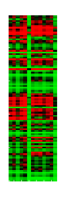
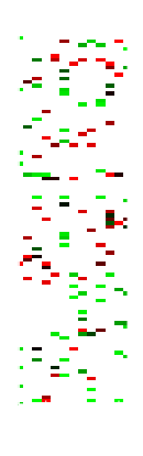
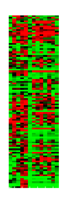
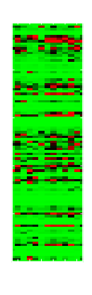
The imputation method (23) is tested here on microarray data described in [27]. Expression levels of yeast across genes sampled at time points during the cell cycle are considered. A subset of genes is extracted and their expression levels are organized in the matrix depicted in Fig. 5 (left). Severe data losses are simulated by discarding of the entries of , including the nearly actually missing data.
According to the Bayesian model (26), it follows that
| (31) |
To study the effect of hydrogen peroxide on the cell cycle arrest, two extra microarray datasets , synchronized with , are collected in [27]. These two matrices are employed to form an estimate of , which is used instead of in (27) after neglecting the noise term in (31). Since the presence of hydrogen peroxide in samples and induces cell cycle arrest, the correlation between samples across time in and is altered, and thus these samples are not appropriate for estimating . Alternatively, the sample estimate of is formed with the microarray data of the genes set aside, and then used in place of in (27).
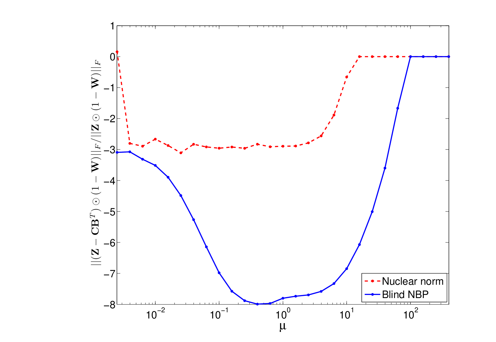
Solving (27) with the available data ( of the total) as shown in Fig. 5 (second left) results in the matrix depicted in Fig. 5 (second right), where the imputed missing data introduce an average recovery error of dB [cf. Fig. 6]. In producing , the smoothing capability of (23) to recover completely missing rows of (amounting to 25 in this example) is corroborated. Missing rows cannot be recovered by nuclear norm regularization alone [cf. (20)], even if is padded with expression levels of the discarded genes. Fig. 5 (right) presents this case confirming that its performance dagrades w.r.t. NBP; while Fig. 6 illustrates the sensitivity of the estimation error to the cross-validated regularization parameter for both estimators. Similar degraded results are observed when imputing missing entries of using the impute.knn() and svdImpute() methods, as implemented in the R packages pcaMethods and BioConductor-impute. These two methods were applied to the padded , after the requisite discarding of the 25 missing rows, resulting in recovery errors on the remaining missing entries at dB and dB (with parameter nPcs), respectively.
VII-C Network Flow Prediction via Blind NBP
The Abilene network in Fig. 7, a.k.a. Internet 2, comprising nodes and links [1], is utilized as a testbed for traffic load prediction. Aggregate link loads are recorded every minute intervals in the morning of December 22, 2008, between 12:00am and 11:55pm, and are collected in the first columns of matrix These samples are then used to predict link loads hours ahead, by capitalizing on their mutual cross-correlation, the periodic correlation across days, and their interdependence across links as dictated by the network topology.
The correlation matrix represented in Fig. 8 is estimated with training samples collected during the two previous weeks, from December 8 to December 21, 2008, and substituted for in (27) according to (31). A singular point at 11:00am in the traffic curve, as depicted in black in Fig. 9, is reflected in the sharp transition noticed in Fig. 8. On the other hand, is not estimated but derived from the network structure. Supposing i.i.d. flows across the network, it holds that , where represents the network routing matrix and the flow variance. Thus, , was used instead of in (27), with adjusted to satisfy .
Fig. 9 shows link loads predicted by (27) on December 22, 2008, for a representative link, along with the actually recorded samples for that day. Prediction accuracy is compared in Fig. 9 to a base strategy comprising independent LMMSE estimators per link, which yield a relative prediction error aggregated across links, against that results from (27). Strong correlation among samples from 12:00am to 2:00pm [cf. Fig. 8] renders LMMSE prediction accurate in this interval, relying on single-link data only. The benefit of considering the links jointly is appreciated in the subsequent interval from 2:00pm to 11:55pm, where the traffic correlation with morning samples fades away and the network structure comes to add valuable information, in the form of , to stabilize prediction.


VIII Summary
A new methodology was outlined in this paper by cross fertilizing sparsity-aware signal processing tools with kernel-based learning. It goes well beyond translating sparse vector regression techniques into their nonparametric counterparts, to generate a series of unique possibilities such as kernel selection or kernel-based matrix completion. The present article contributes to these efforts by advancing NBP as the cornerstone of sparse KBL, including blind versions that emerge as nonparametric nuclear norm regularization and dictionary learning.
KBL was connected with GP analysis, promoting a Bayesian viewpoint where kernels convey prior information. Alternatively, KBL can be regarded as an interpolation toolset though its connection with the NST, suggesting that the impact of the prior model choice is attenuated when the size of the dataset is large, especially when kernel selection is also incorporated.
All in all, sparse KBL was envisioned as a fruitful research direction. Its impact on signal processing practice was illustrated through a diverse set of application paradigms.
Appendix
Proofs of Properties P1-P3
Proof:
1) If white noise is fed to an ideal low-pass filter with cutoff frequency , then is the autocorrelation of the output . Hence, equals the covariance matrix of , and as such . ∎
Proof:
2) Rewrite the kernel as a function parameterized by . Then, the NST applied to the bandlimited yields . ∎
Proof:
3) Upon defining , the reconstruction formula gives the kernel expansion of . Hence, by definition of the RKHS norm . Substituting the reconstructed into the last equation yields . ∎
Design of Algorithm 1
In order to rewrite the cost in terms and , representing the -th columns of matrix and , respectively, define and decompose . Then rewrite the cost as
| (32) |
after defining and discarding regularization terms not depending on .
Let denote the vector operator that concatenates columns of , and the diagonal matrix operator such that . The Hadamard product can be bypassed by defining , substituting , and using the following identities
| (33) |
with representing the Kroneker product. Applying (33) to (32) yields
| (34) |
Equating the gradient of (34) w.r.t. to zero, and solving for it results
| (35) |
References
- [1] [Online]. Available: http://internet2.edu/observatory/archive/data-collections.html.
- [2] IEEE Standard for Info. Tech.-Telecomms. and Info. Exchchange between Systems-Local and Metropolitan Area Nets., Part 11: Wir. LAN MAC and PHY Specifications, IEEE Standard 802.11-2012, pp. 1-1184, Mar. 2012.
- [3] J. Abernethy, F. Bach, T. Evgeniou, and J.-P. Vert, “A new approach to collaborative filtering: Operator estimation with spectral regularization,” J. Machine Learning Res., vol. 10, pp. 803-826, Mar. 2009.
- [4] P. Agrawal and N. Patwari, “Correlated link shadow fading in multihop wireless network,” IEEE Trans. on Wireless Comm., vol. 8, no. 8, pp. 4024-4036, Aug. 2009.
- [5] S. Boyd and L. Vandenberghe, Convex Optimization, Cambridge University Press, 2004.
- [6] J. A. Bazerque, G. Mateos, and G. B. Giannakis, “Group-Lasso on splines for spectrum cartography,” IEEE Trans. on Signal Proc., vol. 59, no. 10, pp. 4648-4663, Oct. 2011.
- [7] J. A. Bazerque, G. Mateos, and G. B. Giannakis, “Nonparametric low-rank tensor imputation,” IEEE Workshop on Stat. Signal Proc., Ann Arbor, MI, Aug. 5-8, 2012.
- [8] E. J. Candes, and T. Tao, “Decoding by linear programming,” IEEE Trans. on Info. Theory, vol. 51, no. 12, pp. 4203-4215, Dec. 2005.
- [9] S. S. Chen, D. L. Donoho, and M. A. Saunders, “Atomic decomposition by basis pursuit,” SIAM J. Sci. Computing, vol. 20, no. 1, pp. 33-61, Dec. 1998.
- [10] N. Cressie, Statistics for Spatial Data, Wiley, 1991.
- [11] J. Duchon, Splines Minimizing Rotation-Invariant Semi-norms in Sobolev Spaces, New York: Springer-Verlag, 1977.
- [12] M. Fazel, “Matrix rank minimization with applications” PhD Thesis, Electrical Engineering Dept., Stanford University, vol. 54, pp. 1-130, 2002.
- [13] Q. Geng and J. Wright, “On the local correctness of -minimization for dictionary learning,” IEEE Trans. on Info. Theory, 2011 (submitted); see arXiv:1101.5672v1 [cs.IT].
- [14] F. Girosi, “An equivalence between sparse approximation and support vector machines,” Neural Computation vol. 10, no. 6, pp. 1455-1480, Aug. 1998.
- [15] R. Gribonval and K. Schnass, “Dictionary identification - sparse matrix factorization via -minimization” IEEE Trans. on Info. Theory, vol. 56, no. 7, pp. 3523 - 3539, July 2010.
- [16] T. Hastie, R. Tibshirani, and J. Friedman, The Elements of Statistical Learning, 2nd ed., Springer, NY, 2009.
- [17] S. Kay, Fundamentals of Statistical Signal Processing, vol. 1, Prentice Hall, 2001.
- [18] V. Kekatos, S. Veeramachaneni, M. Light, and G. B. Giannakis, “Day-ahead electricity market forecasting using kernels,” Proc. of IEEE-PES on Innovative Smart Grid Technologies, Washington, DC, Feb. 24-27, 2013.
- [19] V. Koltchinskii and M. Yuan, “Sparsity in multiple kernel learning,” Annals of Statistics vol. 38, no. 6, pp. 3660-3695, Apr. 2010.
- [20] K. Kreutz-Delgado, J. F. Murray, B. D. Rao, K. Engan, T. W. Lee, and T. J. Sejnowski, “Dictionary learning algorithms for sparse representation,” Neural Computation, vol. 15, no. 2, pp. 349-396, Feb. 2003.
- [21] Y. Lin and H. H. Zhang, “Component selection and smoothing in multivariate nonparametric regression,” Annals of Statistics, vol. 34, no. 5, pp. 2272-2297, May 2006.
- [22] M. Mardani, G. Mateos, and G. B. Giannakis, “In-network sparsity-regularized rank minimization: Algorithms and applications,” IEEE Trans. on Signal Proc., 2012; see also arXiv:1203.1507v1 [cs.MA].
- [23] C. Micchelli and M. Pontil, “Learning the kernel function via regularization,” J. Machine Learning Res., vol. 6, pp. 1099-1125, Sep. 2005.
- [24] M. Z. Nashed and Q. Sun, “Function spaces for sampling expansions,” Multiscale Signal Analysis and Modelling, edited by X. Shen and A. Zayed, Lecture Notes in EE, Springer, pp. 81-104, 2012.
- [25] C. E. Rasmussen and C. K. I. Williams, Gaussian Processes for Machine Learning, the MIT Press, 2006.
- [26] P. Ravikumar, J. Lafferty, H. Liu, and L. Wasserman, “Sparse additive models,” J. Roy. Stat. Soc. B, vol. 71, no. 5, pp. 1009-1030, Oct. 2009.
- [27] M. Shapira, M. E. Segal, and D. Botstein, “Disruption of yeast forkhead-associated cell cycle transcription by oxidative stress,” Molecular Biology of the Cell, vol. 15, no. 12, pp. 5659-5669, Dec. 2004.
- [28] A. Shrivastava, H. V. Nguyen, V. M. Patel, and R. Chellappa, “Design of non-linear discriminative dictionaries for image classification,” Proc. of Asian Conf. on Computer Vision, Daejeon, Korea, 2012.
- [29] V. Sindhwani and A. C. Lozano, “Non-parametric group orthogonal matching pursuit for sparse learning with multiple kernels,” Advances in Neural Information Processing Systems, pp. 2519-2527, Granada, Spain, 2011.
- [30] P. Tseng and S. Yun, “A coordinate gradient descent method for nonsmooth separable minimization,” J. Mathematical Programming, vol. 117, no. 1-2, pp. 387-423, Mar. 2009.
- [31] M. Unser, “Splines: A perfect fit for signal and image processing,” IEEE Signal Proc. Magazine, vol. 16, no. 6, pp. 22-38, Nov. 1999.
- [32] P. Vincent and Y. Bengio, “Kernel matching pursuit,” Machine Learning, vol. 48, pp. 169-191, 2002.
- [33] G. Wahba, Spline Models for Observational Data, Society for Industrial and Applied Mathematics, PA 1990.
- [34] Z. Xing, M. Zhou, A. Castrodad, G. Sapiro and L. Carin, “Dictionary learning for noisy and incomplete hyperspectral images,” SIAM Journal on Imaging Sciences, vol. 5, no. 1, pp. 33-56, 2012.
- [35] Z. Zhang, and B. D. Rao, “Sparse signal recovery with temporally correlated source vectors using sparse Bayesian learning,” IEEE J. Sel. Topics in Signal Proc., vol. 5, no. 5, pp. 912-926, Sep. 2011.