跳到论文正文
W Papers独立论文阅读器 arXiv:1302.5238 论文正文 计算阅读时间 · 0%
引用这篇论文根据当前论文元数据生成,正式投稿前建议核对。


License: arXiv.org perpetual non-exclusive license
arXiv:1302.5238v4 [quant-ph] 14 Mar 2014

Entanglement in two site Bose-Hubbard model

K. V. S. Shiv Chaitanya Email: E-mail: chaitanya@hyderabad.bits-pilani.ac.in Affiliation: BITS Pilani, Hyderabad Campus, Jawahar Nagar,
Shameerpet Mandal, Hyderabad, India 500 078.
   Sibasish Ghosh Email: E-mail: sibasish@imsc.res.in Affiliation: Optics &\& Quantum Information Group,
The Institute of Mathematical Sciences, C.I.T Campus
Taramani, Chennai, India, 600113.
   V. Srinivasan Email:  E-mail:: vsspster@gmail.com Affiliation: Department of Theoretical Physics, University of Madras,
Guindy, Chennai, India, 600025.
Abstract

In this paper, we study the decoherence and entanglement properties for the two site Bose-Hubbard model in the presence of a non-linear damping. We apply the techniques of thermo field dynamics and then use Hartree-Fock approximation to solve the corresponding master equation. The expectation values of the approximated field operators appearing in the solution of master equation, are computed self-consistently. We solve this master equation for a small time tt so that we get the analytical solution, thereby we compute the decoherence and entanglement properties of the solution of the two-mode bosonic system.

I Introduction

In recent years, there is lot of interest generated in the study of entanglement properties of ultra cold atoms [1, 2, 3, 4, 5, 6]. In one such study, the single-site addressability in a two-dimensional optical lattice [7] has been demonstrated which could be a natural resource for applications of quantum information processing with neutral atoms. In all the experimental demonstrations of ultra cold atoms, loss is an important role which gives rise to decoherence and in turn destroying the quantum correlations. The losses due to decoherence can be modelled by a master equation. One such model is examined in the ref [5, 6] for a linear damping using the Bose-Hubbard model. The Bose-Hubbard model [8] is one of the popular model used to study the evolution of cold atoms and the Bose-Einstein condensates in an optical lattice. In this paper, we examin the two-site Bose-Hubbard model to study the entanglement and decoherence properties of two mode states under the action of non-linear damping. We consider the following master equation for density matrix ρ\rho in a non-linear medium

∂∂t​ρ=iℏ​[H,ρ]+κ​∑k=1K([ak​bk,ρ​ak†​bk†]+[ak​bk​ρ,ak†​bk†])\displaystyle\frac{\partial}{\partial t}\rho=\frac{i}{\hbar}[H,\rho]+\kappa\sum_{k=1}^{K}([a_{k}b_{k},\rho a_{k}^{\dagger}b_{k}^{\dagger}]+[a_{k}b_{k}\rho,a_{k}^{\dagger}b_{k}^{\dagger}]) (1)

here κ\kappa is a damping coefficient, aka_{k} and bkb_{k} bosonic annihilation operators referring to atoms in the internal states |N1⟩|N_{1}\rangle and |N2⟩|N_{2}\rangle, respectively, with one boson in the kth lattice site and KK is the number of lattice sites and HH is the Hamiltonian for the Bose-Hubbard model which describes the optical lattice. In this paper, we are studying the model in the presence of non-linear damping corresponding to the term associated with κ\kappa.

For solving this master equation we use the techniques of thermo field dynamics and thereby the Hartree-Fock approximation method to convert the two-site Bose-Hubbard model in eq (1) into a two-mode bosonic system. The two-site Bose-Hubbard model is used to study Josephson tunnelling between two Bose-Einstein condensates (BEC). This toy model can be used to study the BEC. The expectation values of the approximated field is computed self-consistently. We solve the master equation (1) for a small time tt so that we get the analytical solution, thereby we compute the decoherence and entanglement properites of the two-mode bosonic system.

The thermo field dynamics (TFD)[9, 10, 11, 12, 13] is a finite temperature field theory. It is applied to many branches in high energy physics [10] and many-body systems [13]. The thermo field dynamics is used to solve the master equation by in presence of Kerr medium [14, 15] using disentanglement theorem for any arbitrary initial conditions. This formalism, presented in ref [14, 15, 18, 19, 20] has two sailent features, first, solving the master equation is reduced to solving a Schrödinger equation, thus all the techniques available to solve the Schrödinger equation are applicable here. Second, the thermal coherent state under the master equation evolution goes over to a thermal coherent state.

A brief description of TFD is given in appendix D. In TFD, any master equation is given by

∂∂t​|ρ⁡(t)⟩=−i​H^​|ρ⟩\displaystyle\frac{\partial}{\partial t}|\rho(t)\rangle=-i\hat{H}|\rho\rangle (2)

where |ρ⟩|\rho\rangle is a vector in an extended Hilbert space ℋ⊗ℋ∗{\cal H}\otimes{\cal H}^{*} and

−i​H^=i⁡(H−H~)+L.\displaystyle-i\hat{H}=i(H-\tilde{H})+L. (3)

where HH is the Hamiltonian in Hilbert space ℋ{\cal H}, H~\tilde{H} is the Hamiltonian in Hilbert space ℋ∗{\cal H}^{*} and L is the Liouville term, as mentioned in appendix D . Thus, −i​H^-i\hat{H} is tildian and the problem of solving master equation is reduced to solving a Schrödinger like equation namely eq (2). Then, the symmetry associated to the Hamiltonian such as s​u​(1,1)su(1,1) symmetry, are exploited to solve the eq (2) and thereby the master equation.

In this paper, we follow this formalism to solve the master equation(1) for the two site Bose-Hubbard model in the presence of non-linear medium.

This paper is organized as follows. In the section II, we describe the two site Hubbard model. In section III, we describe the solution of corresponding master equation. In section III-A, we discuss the self consistency analysis of the solution for a short initial time. The issue of entanglement of the solution - two mode Gaussian state - is described in section IV. While the issue of decoherence is discussed in section V. In the section VI, we draw conclusions. A few appendices are added to provide the details.

II Two site Bose-Hubbard Model

The Hamiltonian HH of the Bose-Hubbard model, appeared on the RHS of eq (1), describes the interaction of bosons situated on an optical lattice, and is given by

H\displaystyle H =\displaystyle= ω​∑k(ak†​ak+bk†​bk)−J​∑{k,l}(ak†​bl+bk†​al)\displaystyle\omega\sum_{k}(a_{k}^{\dagger}a_{k}+b_{k}^{\dagger}b_{k})-J\sum_{\{k,l\}}(a_{k}^{\dagger}b_{l}+b_{k}^{\dagger}a_{l}) (4)
+Ua2∑kak†ak†akak+Ub2∑kbk†bk†bkbk\displaystyle+\frac{U_{a}}{2}\sum_{k}a_{k}^{\dagger}a_{k}^{\dagger}a_{k}a_{k}+\frac{U_{b}}{2}\sum_{k}b_{k}^{\dagger}b_{k}^{\dagger}b_{k}b_{k}
+Ua​b2∑{k,l}ak†akbl†bl\displaystyle+\frac{U_{ab}}{2}\sum_{\{k,l\}}a_{k}^{\dagger}a_{k}b_{l}^{\dagger}b_{l}

with aka_{k} and bkb_{k} bosonic annihilation operators referring to atoms in the internal states |N1⟩|N_{1}\rangle and |N2⟩|N_{2}\rangle, respectively, with one boson in the kkth lattice site, KK is the number of lattice sites and {k,l}\{k,l\} refers to the adjacent lattice points kk and ll. The interaction term JJ in the Hamiltonian describes the induced hopping between adjacent cells, ω\omega is the frequency of the atom in the lattice. The on-site interactions of atoms are described by the interaction strengths UaU_{a} and UbU_{b}, and a nearest-neighbour interaction by Ua​bU_{ab}. For further details see ref [8]. To study the decoherence and the entanglement properties of Bose-Hubbard model, for simplicity, we consider the toy model, in which the Bose-Hubbard model is written for the two site interaction only (with the respective bosonic annihilation operators being aa and bb). The master equation (1) for the two site Bose-Hubbard Hamiltonian HH (given in (4)) is given by

∂∂t​ρ\displaystyle\frac{\partial}{\partial t}\rho =\displaystyle= −i​ω​(a†​a​ρ−ρ​a†​a)−i​J​(a†​b​ρ−ρ​a†​b)\displaystyle-i\omega(a^{\dagger}a\rho-\rho a^{\dagger}a)-iJ(a^{\dagger}b\rho-\rho a^{\dagger}b) (5)
−i​J​(b†​a​ρ−ρ​b†​a)+i​Ua2​(a†​a†​a​a​ρ−ρ​a†​a†​a​a)\displaystyle-iJ(b^{\dagger}a\rho-\rho b^{\dagger}a)+i\frac{U_{a}}{2}(a^{\dagger}a^{\dagger}aa\rho-\rho a^{\dagger}a^{\dagger}aa)
+i​Ub2​(b†​b†​b​b​ρ−ρ​b†​b†​b​b)−i​ω​(b†​b​ρ−ρ​b​b†)\displaystyle+i\frac{U_{b}}{2}(b^{\dagger}b^{\dagger}bb\rho-\rho b^{\dagger}b^{\dagger}bb)-i\omega(b^{\dagger}b\rho-\rho bb^{\dagger})
+i​Ua​b2​(a†​b†​a​b​ρ−ρ​a†​b†​a​b)\displaystyle+i\frac{U_{ab}}{2}(a^{\dagger}b^{\dagger}ab\rho-\rho a^{\dagger}b^{\dagger}ab)
+κ2​(2​a​b​ρ​a†​b†−a†​b†​a​b​ρ−ρ​a†​b†​a​b).\displaystyle+\frac{\kappa}{2}\left(2ab\rho a^{\dagger}b^{\dagger}-a^{\dagger}b^{\dagger}ab\rho-\rho a^{\dagger}b^{\dagger}ab\right).

At first we consider the special case to solve this master equation in which J=Ua=Ub=0J=U_{a}=U_{b}=0 and Ua​b=UU_{ab}=U (say), which corresponds to the Mott insulating phase. Then the master equation (5) reduces to

∂∂t​ρ\displaystyle\frac{\partial}{\partial t}\rho =\displaystyle= −i​ω​(a†​a​ρ−ρ​a†​a)−i​ω​(b†​b​ρ−ρ​b​b†)\displaystyle-i\omega(a^{\dagger}a\rho-\rho a^{\dagger}a)-i\omega(b^{\dagger}b\rho-\rho bb^{\dagger}) (6)
+i​U2​(a†​b†​a​b​ρ−ρ​a†​b†​a​b)\displaystyle+i\frac{U}{2}(a^{\dagger}b^{\dagger}ab\rho-\rho a^{\dagger}b^{\dagger}ab)
+κ2​(2​a​b​ρ​a†​b†−a†​b†​a​b​ρ−ρ​a†​b†​a​b).\displaystyle+\frac{\kappa}{2}\left(2ab\rho a^{\dagger}b^{\dagger}-a^{\dagger}b^{\dagger}ab\rho-\rho a^{\dagger}b^{\dagger}ab\right).

Now, we apply the thermo field dynamics techniques to convert the master equation (6) into a Schrödinger equation by applying |I⟩|I\rangle from the right to the eq (6):

∂∂t​|ρ⟩=−i​H^​|ρ⟩,\frac{\partial}{\partial t}|\rho\rangle=-i\hat{H}|\rho\rangle, (7)

where |ρ⟩|\rho\rangle pure state in the Hilbert space ℋ⊗ℋ∗{\cal H}\otimes{\cal H}^{*} and the Hamiltonian H^\hat{H} is given by

−i​H^\displaystyle-i\hat{H} =\displaystyle= −i​ω​(a†​a−a~​a~†)−i​ω​(b†​b−b~​b~†)\displaystyle-i\omega(a^{\dagger}a-\tilde{a}\tilde{a}^{\dagger})-i\omega(b^{\dagger}b-\tilde{b}\tilde{b}^{\dagger}) (8)
+i​U2​(a†​b†​a​b−a~​b~​a~†​b~†)\displaystyle+i\frac{U}{2}(a^{\dagger}b^{\dagger}ab-\tilde{a}\tilde{b}\tilde{a}^{\dagger}\tilde{b}^{\dagger})
+κ2​(2​a​b​a~​b~−a†​b†​a​b−a~​b~​a~†​b~†),\displaystyle+\frac{\kappa}{2}\left(2ab\tilde{a}\tilde{b}-a^{\dagger}b^{\dagger}ab-\tilde{a}\tilde{b}\tilde{a}^{\dagger}\tilde{b}^{\dagger}\right),

here the aa, bb are the annihilation operators act on the ℋ{\cal H} and a~\tilde{a} and b~\tilde{b} are the annihilation operators act on the Hilbert space ℋ∗{\cal H}^{*} ( for detail see appendix D).

This master equation (8) is a non-linear equation (because (U,κ)≠(0,0)(U,\kappa)\neq(0,0) here), and in general it is difficult to get an analytical solution of this equation. A way out would be to apply the Hartree-Fock approximation and treat the approximated field self-consistently. In the case of thermo field dynamics, a selfconsistent theory using Hartree-Fock approximation is developed for non linear master equations in presence of the non-linear medium in ref [20]. Applying, Hartree-Fock approximation for each term in (8) as follows

2​a~†​b~†​a~​b~=a~†​b~†​⟨a~​b~⟩+⟨a~†​b~†⟩​a~​b~, 2​a†​b†​a​b=⟨a†​b†⟩​a​b+a†​b†​⟨a​b⟩, 2​a~​b~​a​b=a~​b~​⟨a​b⟩+a​b​⟨a~​b~⟩,\displaystyle 2\tilde{a}^{\dagger}\tilde{b}^{\dagger}\tilde{a}\tilde{b}=\tilde{a}^{\dagger}\tilde{b}^{\dagger}\langle\tilde{a}\tilde{b}\rangle+\langle\tilde{a}^{\dagger}\tilde{b}^{\dagger}\rangle\tilde{a}\tilde{b},\;2a^{\dagger}b^{\dagger}ab=\langle a^{\dagger}b^{\dagger}\rangle ab+a^{\dagger}b^{\dagger}\langle ab\rangle,\;2\tilde{a}\tilde{b}ab=\tilde{a}\tilde{b}\langle ab\rangle+ab\langle\tilde{a}\tilde{b}\rangle, (9)

with ⟨a​b⟩=⟨a~​b~⟩=Δ⁡(t)\langle ab\rangle=\langle\tilde{a}\tilde{b}\rangle=\Delta(t), the Hamiltonian in (8) is decoupled into tildien and non tildian parts

H^\displaystyle\hat{H} =\displaystyle= (H1+H2),\displaystyle(H_{1}+H_{2}), (10)

where

H1\displaystyle H_{1} =\displaystyle= ω⁡(a†​a+b†​b)+i​κ​Δ​(t)4​(a​b−a†​b†)\displaystyle\omega(a^{\dagger}a+b^{\dagger}b)+\frac{i\kappa\Delta(t)}{4}\left(ab-a^{\dagger}b^{\dagger}\right) (11)
−U​Δ​(t)4​(a†​b†+a​b)\displaystyle-\frac{U\Delta(t)}{4}(a^{\dagger}b^{\dagger}+ab)

and

H2\displaystyle H_{2} =\displaystyle= −ω⁡(a~​a~†+b~​b~†)+i​κ​Δ​(t)4​(a~​b~−a~†​b~†)\displaystyle-\omega(\tilde{a}\tilde{a}^{\dagger}+\tilde{b}\tilde{b}^{\dagger})+\frac{i\kappa\Delta(t)}{4}\left(\tilde{a}\tilde{b}-\tilde{a}^{\dagger}\tilde{b}^{\dagger}\right) (12)
−U​Δ1​(t)4​(a~†​b~†+a~​b~).\displaystyle-\frac{U\Delta_{1}(t)}{4}(\tilde{a}^{\dagger}\tilde{b}^{\dagger}+\tilde{a}\tilde{b}).

The solution of (7) is then given by

|ρ(t)⟩=(exp[−i∫dtH1]⊗exp[−i∫dtH2])|ρ(0)⟩,|\rho(t)\rangle=\big(exp[-i\int dtH_{1}]\otimes exp[-i\int dtH_{2}]\big)|\rho(0)\rangle, (13)

where |ρ⁡(0)⟩|\rho(0)\rangle is an initial state in ℋ⊗ℋ∗{\cal H}\otimes{\cal H}^{*}.

It is clear from the above that the two Hamiltonians H1H_{1} and H2H_{2} are independent in the sense that H1H_{1} is acting on non-tildian system and H2H_{2} is acting on tildian system Hence, we can work with one of the Hamiltonians and similar thing works for the other Hamiltonian (exept for interchanging between ω\omega and −ω-\omega).

To study the decoherence and entanglement properties of the two-mode states under the action of the master equation (6),(equivalently, the Schrödinger equation (7)), we would like to exploit the underlying symmetry associated with the Hamiltonians (11) and (12). This is accomplished by defining the following operators :

𝒩\displaystyle\mathcal{N} =\displaystyle= a†​a+b†​b,𝒦+=a†​b†,𝒦−=a​b\displaystyle a^{\dagger}a+b^{\dagger}b,\;\mathcal{K}_{+}=a^{\dagger}b^{\dagger},\;\mathcal{K}_{-}=ab (14)
𝒩~\displaystyle\tilde{\mathcal{N}} =\displaystyle= a~​a~†+b~​b~†,𝒦~+=a~†​b~†,𝒦~−=a~​b~\displaystyle\tilde{a}\tilde{a}^{\dagger}+\tilde{b}\tilde{b}^{\dagger},\;\tilde{\mathcal{K}}_{+}=\tilde{a}^{\dagger}\tilde{b}^{\dagger},\;\tilde{\mathcal{K}}_{-}=\tilde{a}\tilde{b} (15)

which satisfy the s​u​(1,1)su(1,1) algebra

[𝒩,𝒦+]\displaystyle[\mathcal{N},\mathcal{K}_{+}] =\displaystyle= 𝒦+,[𝒩,𝒦−]=𝒦−,[𝒦+,𝒦−]=2​𝒩.\displaystyle\mathcal{K}_{+},\;[\mathcal{N},\mathcal{K}_{-}]=\mathcal{K}_{-},\;[\mathcal{K}_{+},\mathcal{K}_{-}]=2\mathcal{N}. (16)

Similar algebra holds for tildians operators. Rewriting the Hamiltonian (11) in terms of the s​u​(1,1)su(1,1) generators one gets

−i​H1\displaystyle-iH_{1} =\displaystyle= −i​ω​𝒩+κ​Δ​(t)2​(𝒦−−𝒦+)+i​U​Δ​(t)2​(𝒦++𝒦−),\displaystyle-i\omega\mathcal{N}+\frac{\kappa\Delta(t)}{2}\left(\mathcal{K}_{-}-\mathcal{K}_{+}\right)+i\frac{U\Delta(t)}{2}(\mathcal{K}_{+}+\mathcal{K}_{-}), (17)

and similarly the Hamiltonian (12). It is clear that these two Hamiltonians are associated with the s​u​(1,1)su(1,1) symmetry. Hence, the underlying symmetry of the Schrödinger equation (7) is s​u​(1,1)×s​u​(1,1)su(1,1)\times su(1,1). One of the important features of this s​u​(1,1)su(1,1) symmetry is that it gives rise to squeezing, and in turn, it gives rise to entanglement. If the initial state ρ⁡(0)\rho(0) is a two-mode Gaussian state then, under the action of two-mode squeezing, the final state turns out to be also a Gaussian state. Thus, one can use the separability criterion for Gaussian states [23] to check for the entanglement of the time evolved state ρ⁡(t)\rho(t).

III Solution of Master Equation

To get the solution to the Schrödinger equation (7) we use the Hartree-Fock approximation and treat the approximated field as background field, and the later has to be computed self-consistently in order to get the solution of (7). For doing a self-consistent analysis we first exactly diagonalize the Hamiltonians in eqs (11) and (12) with the help of the underlying s​u​(1,1)su(1,1) symmetry. It is evident form the eqs (11) and (12) that the Hamiltonian in eq (7) is decoupled into tildien and non tildien parts as mentioned in eq (10). Hence, we work with one of the Hamiltonians and similar analysis goes through for the other Hamiltonian. By considering the Hamiltonian

H1\displaystyle H_{1} =\displaystyle= ω⁡(a†​a+b†​b)+i​κ​Δ​(t)2​(a​b−a†​b†)\displaystyle\omega(a^{\dagger}a+b^{\dagger}b)+\frac{i\kappa\Delta(t)}{2}\left(ab-a^{\dagger}b^{\dagger}\right) (18)
−U​Δ​(t)2​(a†​b†+a​b),\displaystyle-\frac{U\Delta(t)}{2}(a^{\dagger}b^{\dagger}+ab),

and applying the following transformation among the mode operators

A\displaystyle A =\displaystyle= μ​a+ν∗​b†,A†=μ∗​a†+ν​b\displaystyle\mu a+\nu^{*}b^{\dagger},\;A^{\dagger}=\mu^{*}a^{\dagger}+\nu b (19)
B\displaystyle B =\displaystyle= μ​b+ν∗​a†,B†=μ∗​b†+ν​a\displaystyle\mu b+\nu^{*}a^{\dagger},\;B^{\dagger}=\mu^{*}b^{\dagger}+\nu a (20)

with μ=ei​ϕμ​|μ|\mu=e^{i\phi_{\mu}}|\mu| and ν=ei​ϕν​|ν|\nu=e^{i\phi_{\nu}}|\nu|, (ϕμ,ϕν∈R\phi_{\mu},\phi_{\nu}\in R), we diagonalize the Hamiltonian H1H_{1}. Similar analysis goes through for the other Hamiltonian H2H_{2}. With a bit of algebra for κ=0\kappa=0, one can exactly diagonalize the Hamiltonian (18) by using the transformations (19) and (20) . Let κ=0\kappa=0 for t=0t=0, then we evolve the state through the schrödinger (7) at this time. Then the corresponding non-tildien Hamiltonian H0H_{0} is given by

H0\displaystyle H_{0} =\displaystyle= ω⁡(a†​a+b†​b)−U​Δ​(t)2​(a†​b†+a​b),\displaystyle\omega(a^{\dagger}a+b^{\dagger}b)-\frac{U\Delta(t)}{2}(a^{\dagger}b^{\dagger}+ab), (21)

and the final diagonalized Hamiltonian HfH_{f} (which is diagonalized version of H0H_{0}), after the unitary transformation (19) and (20), is given by

Hf=S−1​(r)​H0​S​(r)=Ω2​[A†​A+B†​B+1]\displaystyle H_{f}=S^{-1}(r)H_{0}S(r)=\Omega^{2}[A^{\dagger}A+B^{\dagger}B+1] (22)

where

S⁡(r)=e​x​p​[r​𝒦−−r∗​𝒦+]=e​x​p​[r​a†​b†−r∗​a​b]\displaystyle S(r)=exp[r\mathcal{K}_{-}-r^{*}\mathcal{K}_{+}]=exp[ra^{\dagger}b^{\dagger}-r^{*}ab] (23)

here Ω2=4​ω2−U2​Δ2​(0)\Omega^{2}=4\omega^{2}-U^{2}\Delta^{2}(0) and rr is related to μ\mu and ν\nu in eq (19) and (20) via the following Bogolyubov coefficients :

μ=c​o​s​h​(r)\displaystyle\mu=cosh(r) =\displaystyle= ωω2−U2​Δ2​(0)4,\displaystyle\frac{\omega}{\sqrt{\omega^{2}-\frac{U^{2}\Delta^{2}(0)}{4}}},
ν=s​i​n​h​(r)\displaystyle\nu=sinh(r) =\displaystyle= U​Δ​(0)2​ω2−U2​Δ2​(0)4.\displaystyle\frac{U\Delta(0)}{2\sqrt{\omega^{2}-\frac{U^{2}\Delta^{2}(0)}{4}}}. (24)

Note that here

|μ|2−|ν|2=1.\displaystyle|\mu|^{2}-|\nu|^{2}=1. (25)

This fixes Δ2​(0)=ω2+1U2=\Delta^{2}(0)=\frac{\omega^{2}+1}{U^{2}}=Constant. The solution to the Schrödinger equation

i​ℏ​∂∂t​|ψ0​(t)⟩=−i​H0​|ψ0​(t)⟩i\hbar\frac{\partial}{\partial t}|\psi_{0}(t)\rangle=-iH_{0}|\psi_{0}(t)\rangle (26)

where Hamiltonian H0H_{0} is given by eq (21), is given by

|ψ0​(t)⟩\displaystyle|\psi_{0}(t)\rangle =\displaystyle= e​x​p​[r​𝒦−−r∗​𝒦+]​|ψ0​(0)⟩\displaystyle exp[r\mathcal{K}_{-}-r^{*}\mathcal{K}_{+}]|\psi_{0}(0)\rangle (27)
=\displaystyle= e​x​p​[r​a†​b†−r∗​a​b]​|ψ0​(0)⟩.\displaystyle exp[ra^{\dagger}b^{\dagger}-r^{*}ab]|\psi_{0}(0)\rangle.

Similar solution exists for the H~0\tilde{H}_{0} where

H~0\displaystyle\tilde{H}_{0} =\displaystyle= ω⁡(a~†​a~+b~†​b~)−U​Δ​(t)2​(a~†​b~†+a~​b~).\displaystyle\omega(\tilde{a}^{\dagger}\tilde{a}+\tilde{b}^{\dagger}\tilde{b})-\frac{U\Delta(t)}{2}(\tilde{a}^{\dagger}\tilde{b}^{\dagger}+\tilde{a}\tilde{b}). (28)

III.1 Self Consistency Analysis

After achiving the solution of the Schrödinger (7) without the non-linearity (as say κ=0\kappa=0), we now compute the background field Δ⁡(t)\Delta(t) self-consistently by taking the initial state of the two-mode system to be the vacuum state. The aim is to reinforce the non-linearity. In thermo field dynamic notation the two-mode vacuum state is given by |ρ(0)⟩=|00,0~0~⟩|\rho(0)\rangle=|00,\tilde{0}\tilde{0}\rangle, while in the usual notation ρ(t)=e−i∫dtH^|0,0⟩⟨0,0|ei​∫d​t​H^\rho(t)=e^{-i\int dt\hat{H}}|0,0\rangle\langle 0,0|e^{i\int dt\hat{H}}. In thermo field dynamics, the background field Δ⁡(t)\Delta(t) is computed as expectation value of the averaged creation and annihilation operators, and is given by

Δ⁡(t)=⟨a​b⟩=⟨I|a​b|ρ⁡(t)⟩=T​r​(a​b​ρ​(t)).\Delta(t)=\langle ab\rangle=\langle I|ab|\rho(t)\rangle=Tr(ab\rho(t)). (29)

After doing a bit of algebra (see Appendix B) one gets Δ⁡(t)\Delta(t) to be

Δ⁡(t)\displaystyle\Delta(t) =\displaystyle= (1+i​ω​t)​C​Δ​(0)+(1+n¯1​n¯2)​(U−i​κ)2​∫0td​t′​Δ​(t′)​s​i​n​h2​(C​Δ​(0)​t).\displaystyle(1+i\omega t)C\Delta(0)+\left(1+\bar{n}_{1}\bar{n}_{2}\right)\frac{(U-i\kappa)}{2}\int_{0}^{t}dt^{\prime}\Delta(t^{\prime})sinh^{2}(C\Delta(0)t). (30)

where c=Uωc=\frac{U}{\omega}. This is nothing but the Fredholm integral equation of the second kind. Computing the integral upto first order one gets

Δ⁡(t)\displaystyle\Delta(t) =\displaystyle= (1+i​ω​t)​C​Δ​(0)−(1+n¯1​n¯2)​(U−i​κ)​(1−i​ω)2​[λ​t2−λ2​Ω​s​i​n​h​(C​Δ​(0)​t)].\displaystyle(1+i\omega t)C\Delta(0)-\left(1+\bar{n}_{1}\bar{n}_{2}\right)\frac{(U-i\kappa)(1-i\omega)}{2}[\frac{\lambda t}{2}-\frac{\lambda}{2\Omega}sinh(C\Delta(0)t)]. (31)

By considering Ω​t\Omega t to be small (so that OPENs​i​n​h​(C​Δ​(0)​t)≃C​Δ​(0)​t)sinh(C\Delta(0)t)\simeq C\Delta(0)t) one gets

Δ⁡(t)=(1+i​ω​t)​C​Δ​(0).\displaystyle\Delta(t)=(1+i\omega t)C\Delta(0). (32)

Hence the solution of the Schrödinger equation (7) is given by eq (13), which when written in terms of the s​u​(1,1)su(1,1) generators, becomes

|ρ⁡(t)⟩\displaystyle|\rho(t)\rangle =\displaystyle= (e​x​p​[ζa​3​𝒩+ζa−​𝒦−+ζa+​𝒦+]CLOSE\displaystyle\Big(exp[\zeta_{a3}\mathcal{N}+\zeta_{a-}\mathcal{K}_{-}+\zeta_{a+}\mathcal{K}_{+}] (33)
⊗exp[ζb​3𝒩~+ζb−𝒦~−+ζb+𝒦~+])|ρ(0)⟩,\displaystyle\otimes exp[\zeta_{b3}\tilde{\mathcal{N}}+\zeta_{b-}\tilde{\mathcal{K}}_{-}+\zeta_{b+}\tilde{\mathcal{K}}_{+}]\Big)|\rho(0)\rangle,

where ζa​3=i​ω​t\zeta_{a3}=i\omega t, ζa−=∫d​t​Δ⁡(t)2​(i​U+κ)\zeta_{a-}=\int dt\frac{\Delta(t)}{2}(iU+\kappa), ζa+=∫d​t​Δ⁡(t)2​(i​U−κ)\zeta_{a+}=\int dt\frac{\Delta(t)}{2}(iU-\kappa), ζb​3=i​ω​t\zeta_{b3}=i\omega t, ζb−=∫d​t​Δ⁡(t)2​(i​U+κ)\zeta_{b-}=\int dt\frac{\Delta(t)}{2}(iU+\kappa) and ζb+=∫d​t​Δ⁡(t)2​(i​U−κ)\zeta_{b+}=\int dt\frac{\Delta(t)}{2}(iU-\kappa). Using the disentanglement formula [22] one can write eq (33) as

|ρ⁡(t)⟩\displaystyle|\rho(t)\rangle =\displaystyle= {(exp[Γa+𝒦+]exp[ln(Γa​3𝒩]exp[Γa−𝒦−])⊗\displaystyle\big\{\left(exp[\Gamma_{a+}\mathcal{K}_{+}]exp[ln(\Gamma_{a3}\mathcal{N}]exp[\Gamma_{a-}\mathcal{K}_{-}]\right)\otimes (34)
(exp[Γb+𝒦~+]exp[ln(Γb​3𝒩~)]exp[Γb−𝒦~−])}\displaystyle\left(exp[\Gamma_{b+}\tilde{\mathcal{K}}_{+}]exp[ln(\Gamma_{b3}\tilde{\mathcal{N}})]exp[\Gamma_{b-}\tilde{\mathcal{K}}_{-}]\right)\big\}
|ρ⁡(0)⟩.\displaystyle|\rho(0)\rangle.

where

Γi±\displaystyle\Gamma_{i\pm} =\displaystyle= 2​ζi±​s​i​n​h​ϕi2​ϕi​c​o​s​h​ϕi−ζi​3​s​i​n​h​ϕi,\displaystyle\frac{2\zeta_{i\pm}sinh\phi_{i}}{2\phi_{i}cosh\phi_{i}-\zeta_{i3}sinh\phi_{i}},
Γi​3\displaystyle\Gamma_{i3} =\displaystyle= 1(c​o​s​h​ϕi−ζi​32​ϕi​s​i​n​h​ϕi)2\displaystyle\frac{1}{\left(cosh\phi_{i}-\frac{\zeta_{i3}}{2\phi_{i}}sinh\phi_{i}\right)^{2}} (35)

with

ϕi2\displaystyle\phi_{i}^{2} =\displaystyle= ζi​324−ζi+​ζi−\displaystyle\frac{\zeta_{i3}^{2}}{4}-\zeta_{i+}\zeta_{i-} (36)

and ii stands for aa and bb.

It can be clearly seen that the Γi\Gamma_{i}’s are functions of the background field Δ⁡(t)\Delta(t). By using the expression for Δ⁡(t)\Delta(t) from eq (32) (which is valid for small tt) we get

Γi±\displaystyle\Gamma_{i\pm} =\displaystyle= Δ⁡(0)​t2​(i​U±κ)​(1+ω2​t24).\displaystyle\frac{\Delta(0)t}{2}(iU\pm\kappa)(1+\frac{\omega^{2}t^{2}}{4}). (37)

By taking (i​U±κ)=−ζ​ei​ϕ(iU\pm\kappa)=-\zeta e^{i\phi} then one gets

Γi±\displaystyle\Gamma_{i\pm} =\displaystyle= −Δ⁡(0)​ζ​t2​(1+ω2​t24)​e±i​ϕ.\displaystyle-\frac{\Delta(0)\zeta t}{2}(1+\frac{\omega^{2}t^{2}}{4})e^{\pm i\phi}. (38)

By considering any arbitrary initial state ρ(0)=∑m,n∞ρm,m′,n.n′|m,m′⟩⟨n,n′|\rho(0)=\sum_{m,n}^{\infty}\rho_{m,m^{\prime},n.n^{\prime}}|m,m^{\prime}\rangle\langle n,n^{\prime}| of a single mode system where |m,m′⟩|m,m^{\prime}\rangle and |n,n′⟩|n,n^{\prime}\rangle are number of states, in the thermo field dynamic notation, there by using eq(111) (of appendix D), |ρ⁡(0)⟩|\rho(0)\rangle takes the form

|ρ(0)⟩=∑m,n∞ρm,n(0)|m,m′,n,n′⟩.\displaystyle|\rho(0)\rangle=\sum_{m,n}^{\infty}\rho_{m,n}(0)|m,m^{\prime},n,n^{\prime}\rangle. (39)

Putting eq (39)in (34) one gets

ρm,n​(t)\displaystyle\rho_{m,n}(t) =\displaystyle= ∑q′=0m​i​n​(m′,n′)∑p′=0∞[(m′+p′−q′p′)​(n′+p′−q′p′)​(m′q′)​(n′q′)]12\displaystyle\sum_{q^{\prime}=0}^{min(m^{\prime},n^{\prime})}\sum_{p^{\prime}=0}^{\infty}\left[\left(\begin{array}[]{c}m^{\prime}+p^{\prime}-q^{\prime}\\ p^{\prime}\end{array}\right)\left(\begin{array}[]{c}n^{\prime}+p^{\prime}-q^{\prime}\\ p^{\prime}\end{array}\right)\left(\begin{array}[]{c}m^{\prime}\\ q^{\prime}\end{array}\right)\left(\begin{array}[]{c}n^{\prime}\\ q^{\prime}\end{array}\right)\right]^{\frac{1}{2}} (58)
×∑q=0m​i​n​(m,n)∑p=0∞[(m+p−qp)​(n+p−qp)​(mq)​(nq)]12\displaystyle\times\sum_{q=0}^{min(m,n)}\sum_{p=0}^{\infty}\left[\left(\begin{array}[]{c}m+p-q\\ p\end{array}\right)\left(\begin{array}[]{c}n+p-q\\ p\end{array}\right)\left(\begin{array}[]{c}m\\ q\end{array}\right)\left(\begin{array}[]{c}n\\ q\end{array}\right)\right]^{\frac{1}{2}}
×[Γa+]p′​[Γa​3](m′+n′−2​q′+1)/2​[Γa−]q′​[Γb+]p​[Γb​3](m+n−2​q+1)/2​[Γb−]q\displaystyle\times[\Gamma_{a+}]^{p^{\prime}}[\Gamma_{a3}]^{(m^{\prime}+n^{\prime}-2q^{\prime}+1)/2}[\Gamma_{a-}]^{q^{\prime}}[\Gamma_{b+}]^{p}[\Gamma_{b3}]^{(m+n-2q+1)/2}[\Gamma_{b-}]^{q}
×ρm+p−q,m′+p′−q′,n+p−q+n′+p′−q′​(0).\displaystyle\times\rho_{m+p-q,m^{\prime}+p^{\prime}-q^{\prime},n+p-q+n^{\prime}+p^{\prime}-q^{\prime}}(0).

IV Entanglement

The solution of the Schrödinger equation (7) is a pure state in the thermo field dynamic notation and is given by

|ρ⁡(t)⟩\displaystyle|\rho(t)\rangle =\displaystyle= (exp[Γa+𝒦+]exp[ln(Γa​3𝒩]exp[Γa−𝒦−]\displaystyle\big(exp[\Gamma_{a+}\mathcal{K}_{+}]exp[ln(\Gamma_{a3}\mathcal{N}]exp[\Gamma_{a-}\mathcal{K}_{-}] (59)
×exp[Γb+𝒦~+]exp[ln(Γb​3𝒩~)]exp[Γb−𝒦~−])\displaystyle\times exp[\Gamma_{b+}\tilde{\mathcal{K}}_{+}]exp[ln(\Gamma_{b3}\tilde{\mathcal{N}})]exp[\Gamma_{b-}\tilde{\mathcal{K}}_{-}]\big)
|ρ⁡(0)⟩.\displaystyle|\rho(0)\rangle.

where Γi±\Gamma_{i\pm} are given in eq (38) and K±K_{\pm} are given in eq (14) and (15). In this Schrödinger equation, as there is no mixing between the tildian and non-tildian modes in the Liouville space, one can write the solution in the system Hilbert space as

ρ⁡(t)\displaystyle\rho(t) =\displaystyle= (exp[Γa+𝒦+]exp[ln(Γa​3𝒩]exp[Γa−𝒦−])ρ(0)(exp[Γa+𝒦+]exp[ln(Γa​3𝒩]exp[Γa−𝒦−])\displaystyle\big(exp[\Gamma_{a+}\mathcal{K}_{+}]exp[ln(\Gamma_{a3}\mathcal{N}]exp[\Gamma_{a-}\mathcal{K}_{-}]\big)\rho(0)\big(exp[\Gamma_{a+}\mathcal{K}_{+}]exp[ln(\Gamma_{a3}\mathcal{N}]exp[\Gamma_{a-}\mathcal{K}_{-}]\big) (60)

where again Γi±\Gamma_{i\pm} are given in eq (38) and ρ⁡(0)\rho(0) is the initial state of two mode system. One can clearly see that this a two-mode squeezed state of the two-mode Hilbert space. It is well known that two-mode squeezing gives rises to entanglement. As an example, we take the initial state ρ⁡(0)\rho(0) to be the two-mode thermal state. Then, to calculate the entanglement of the time evolved state ρ⁡(t)\rho(t) we go over to phase space description by following transformation

a\displaystyle a =\displaystyle= 12​(x+i​px),a†=12​(x−i​px),\displaystyle\frac{1}{\sqrt{2}}(x+ip_{x}),\;a^{\dagger}=\frac{1}{\sqrt{2}}(x-ip_{x}), (61)
b\displaystyle b =\displaystyle= 12​(y+i​py),b†=12​(y−i​py).\displaystyle\frac{1}{\sqrt{2}}(y+ip_{y}),\;b^{\dagger}=\frac{1}{\sqrt{2}}(y-ip_{y}). (62)

Putting them in the eq (60) one gets the two-mode squeezed thermal state in the phase space corresponding to the two-mode the real squeezing transformation

S⁡(r)=(c​o​s​h​(r)0s​i​n​h​(r)00c​o​s​h​(r)0−s​i​n​h​(r)s​i​n​h​(r)0c​o​s​h​(r)00−s​i​n​h​(r)0c​o​s​h​(r)),S(r)=\left(\begin{array}[]{cccc}cosh(r)&0&sinh(r)&0\\ 0&cosh(r)&0&-sinh(r)\\ sinh(r)&0&cosh(r)&0\\ 0&-sinh(r)&0&cosh(r)\end{array}\right), (63)

where the squeezing parameter is given by

r=Δ⁡(0)2​(1+ω2​t24)​ζ​t.\displaystyle r=\frac{\Delta(0)}{2}(1+\frac{\omega^{2}t^{2}}{4})\zeta t. (64)

The covariance matrix of a two-mode thermal state is given by

σ=n1​𝟙⊕n2​𝟙\sigma=n_{1}\mathbb{1}\oplus n_{2}\mathbb{1} (65)

where the n1n_{1} and n2n_{2} are sympletic eigenvalues of the covariance matrix. The covariance matrix for the state ρ⁡(t)\rho(t) in eq (60)is given by

V=S⁡(r)​σ​S†​(r)V=S(r)\sigma S^{\dagger}(r) (66)

and so

V=(p0−s00p0s−s0q00s0q)V=\left(\begin{array}[]{cccc}p&0&-s&0\\ 0&p&0&s\\ -s&0&q&0\\ 0&s&0&q\end{array}\right) (67)

with p=n1​c​o​s​h2​(r)+n2​s​i​n​h2​(r)p=n_{1}cosh^{2}(r)+n_{2}sinh^{2}(r), q=n1​s​i​n​h2​(r)+n2​c​o​s​h2​(r)q=n_{1}sinh^{2}(r)+n_{2}cosh^{2}(r) and s=±n1+n22​s​i​n​h​(2​r)s=\pm\frac{n_{1}+n_{2}}{2}sinh(2r).

So the covariance matrix is of the form

V=(ACCTB)V=\left(\begin{array}[]{cc}A&C\\ C^{T}&B\end{array}\right) (68)

where

A=(p00p),B=(q00q),\displaystyle A=\left(\begin{array}[]{cc}p&0\\ 0&p\end{array}\right),\;B=\left(\begin{array}[]{cc}q&0\\ 0&q\end{array}\right),
C=(−s00s),J=(01−10)\displaystyle C=\left(\begin{array}[]{cc}-s&0\\ 0&s\end{array}\right),\;J=\left(\begin{array}[]{cc}0&1\\ -1&0\end{array}\right)

Then the separability condition [23] for any two-mode state reads as

d​e​t​A​d​e​t​B+(14−|d​e​t​C|)2−t​r​(A​J​C​J​B​J​CT​J)≥14​(d​e​t​A+d​e​t​B)detAdetB+\left(\frac{1}{4}-|detC|\right)^{2}-tr(AJCJBJC^{T}J)\geq\frac{1}{4}(detA+detB) (79)

So, the state ρ⁡(t)\rho(t) in eq (60) is entangled if and only if the condition in eq (79) is satisfied. Then the thermal state is entangled iff

s​i​n​h2​(r)≥(n22−1)​(n12−1)(n1+n2)2.sinh^{2}(r)\geq\frac{(n_{2}^{2}-1)(n_{1}^{2}-1)}{(n_{1}+n_{2})^{2}}. (80)

For n1=n2=nn_{1}=n_{2}=n, the amount of entanglement in ρ⁡(t)\rho(t) is given in terms of logarithmic negativity

EN​(r)=−12​[l​o​g2​(e−4​r/n)].E_{N}(r)=-\frac{1}{2}[log_{2}(e^{-4r}/n)]. (81)

V Decoherence

As we have seen the previous section, that the solution to ρ⁡(t)\rho(t) of the master equation (6) in the Hilbert space HH is given by eq (60) and Γi±\Gamma_{i\pm} are given in eq (38). To calculate decoherence effects of ρ⁡(t)\rho(t) we compute ρ2\rho^{2} and is given below. Note that

ρ⁡(t)\displaystyle\rho(t) =\displaystyle= e​x​p​[−Δ⁡(0)​2​(1+ω2​t24)​ζ​t]​ρ​(0)\displaystyle exp[-\Delta(0){2}(1+\frac{\omega^{2}t^{2}}{4})\zeta t]\rho(0) (82)

Then

T​r​[ρ2​(t)]\displaystyle Tr[\rho^{2}(t)] =\displaystyle= T​r​[∑m,n⟨m,n​|ρ2​(t)|​m,n⟩]\displaystyle Tr[\sum_{m,n}\langle m,n|\rho^{2}(t)|m,n\rangle] (83)
=\displaystyle= e​x​p​[−Δ⁡(0)​2​(1+ω2​t24)​ζ​t]\displaystyle exp[-\Delta(0){2}(1+\frac{\omega^{2}t^{2}}{4})\zeta t]

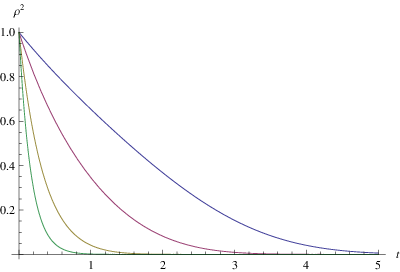
The behaviour of decoherence is plotted fig. 2. One can see immediately that for the short time itself as the value of damping coefficient increases the system decoheres faster.
Refer to caption
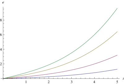
Figure 1: Time vs Entanglement: Here ω=.25\omega=.25, Δ⁡(0)=.25\Delta(0)=.25 and n=.5n=.5 the curves from bottom to top corresponds to ζ=0.1,0.25,0.5​a​n​d​0.75\zeta=0.1,~0.25,~0.5~and~0.75. We use eq (64) and eq (81)
Refer to caption
Figure 2: Time vs Decoherence: Here ω=0.25\omega=0.25 Δ⁡(0)=0.25\Delta(0)=0.25 curves from top to bottom corresponds to ζ=1,0.75,0.5​a​n​d​0.25\zeta=1,~0.75,~0.5~and~0.25.

VI Conclusion

In this paper, the techniques of thermo field dynamics and the Hartree-Fock approximation are used to solve the master equation for the special case of two-mode Bose-Hubbard model in the presence of a non-linear damping. We have treated the approximated field self-consistently and computed it for a small time tt analytically. Then, the decoherence and the entanglement for this system are computed. We show that the entanglement for this system for a short time increases when the initial state is in two-mode thermal state. We interpret this behaviour due to the existence of the non-linear medium. To get the exact picture for the behaviour of the entanglement for a long time, one has to do the numerical studies. For the large time tt we expect the initial state to damp much faster due to the presence of non-linear damping. It can be seen form the decoherecnce plot that as the value of the damping coefficient increases the damping in the system is faster, as expected. We expect that the further numerical studies using this model will give better results and these results may be applied to condensed matter systems.

VII Appendix

VII.1 Appendix A: Calculation of Bogolyubov Coefficients

Consider the following Hamiltonian

H0\displaystyle H_{0} =\displaystyle= ω⁡(a†​a+b†​b)−U​Δ​(t)2​(a†​b†+a​b),\displaystyle\omega(a^{\dagger}a+b^{\dagger}b)-\frac{U\Delta(t)}{2}(a^{\dagger}b^{\dagger}+ab), (84)

By applying the following Bogolyubov or squeezing transformation

A\displaystyle A =\displaystyle= μ​a+ν∗​b†,A†=μ∗​a†+ν​b\displaystyle\mu a+\nu^{*}b^{\dagger},\;A^{\dagger}=\mu^{*}a^{\dagger}+\nu b
B\displaystyle B =\displaystyle= μ​b+ν∗​a†,B†=μ∗​b†+ν​a\displaystyle\mu b+\nu^{*}a^{\dagger},\;B^{\dagger}=\mu^{*}b^{\dagger}+\nu a

(where μ=ei​ϕμ​|μ|\mu=e^{i\phi_{\mu}}|\mu| and ν=ei​ϕν​|ν|\nu=e^{i\phi_{\nu}}|\nu|), we diagonalize the Hamiltonian H0H_{0}. Let us first rewrite the Hamiltonian in a convenient form as

H0=[a†​b]​(mnnm)​[ab†]H_{0}=[a^{\dagger}~~b]\left(\begin{array}[]{cc}m&n\\ n&m\end{array}\right)\left[\begin{array}[]{c}a\\ b^{\dagger}\end{array}\right] (85)

where m=i​ωm=i\omega and n=−i​U​Δ​(0)2n=\frac{-iU\Delta(0)}{2}. By identifying the coefficient matrix appearing in the eq (85) with

(mnnm)=(c​o​s​h​(r)s​i​n​h​(r)s​i​n​h​(r)c​o​s​h​(r)),\left(\begin{array}[]{cc}m&n\\ n&m\end{array}\right)=\left(\begin{array}[]{cc}cosh(r)&sinh(r)\\ sinh(r)&cosh(r)\end{array}\right), (86)

and with a suitable normalization |m|2−|n|2\sqrt{|m|^{2}-|n|^{2}}, the Bogolyubov coefficients can be read off as follows

μ=c​o​s​h​(r)\displaystyle\mu=cosh(r) =\displaystyle= ω2​ω2−U2​Δ2​(0)4,\displaystyle\frac{\omega}{2\sqrt{\omega^{2}-\frac{U^{2}\Delta^{2}(0)}{4}}}, (87)
ν=s​i​n​h​(r)\displaystyle\nu=sinh(r) =\displaystyle= U​Δ​(0)2​ω2−U2​Δ2​(0)4.\displaystyle\frac{U\Delta(0)}{2\sqrt{\omega^{2}-\frac{U^{2}\Delta^{2}(0)}{4}}}. (88)

The above two quantities satisfy

|μ|2−|ν|2=1.\displaystyle|\mu|^{2}-|\nu|^{2}=1. (89)

VII.2 Appendix B: Computation of Δ⁡(t)\Delta(t)

Consider the following field variable appeared in eq (11) and (12)

Δ⁡(t)=⟨a​b⟩\Delta(t)=\langle ab\rangle (90)

The initial state being the thermal state in usual notation

ρ(t)=∑n,m=0∞n¯1n(n¯1+1)n+1n¯2m(n¯2+1)m+1e−i∫dtH|n,m⟩⟨n,m|ei​∫d​t​H\rho(t)=\sum_{n,m=0}^{\infty}\frac{\bar{n}_{1}^{n}}{(\bar{n}_{1}+1)^{n+1}}\frac{\bar{n}_{2}^{m}}{(\bar{n}_{2}+1)^{m+1}}e^{-i\int dtH}|n,m\rangle\langle n,m|e^{i\int dtH} where HH is is equal to H1H_{1} in eq (11). So we have

⟨a​b⟩\displaystyle\langle ab\rangle =\displaystyle= ⟨I|a​b|ρ⁡(t)⟩=T​r​(a​b​ρ​(t))\displaystyle\langle I|ab|\rho(t)\rangle=Tr(ab\rho(t))
=\displaystyle= ∑n,m=0∞n¯1n(n¯1+1)n+1n¯2m(n¯2+1)m+1Tr(abe−i∫dtH|n,m⟩⟨n,m|ei​∫d​t​H)\displaystyle\sum_{n,m=0}^{\infty}\frac{\bar{n}_{1}^{n}}{(\bar{n}_{1}+1)^{n+1}}\frac{\bar{n}_{2}^{m}}{(\bar{n}_{2}+1)^{m+1}}Tr(abe^{-i\int dtH}|n,m\rangle\langle n,m|e^{i\int dtH})
=\displaystyle= ∑n,m=0∞n¯1n(n¯1+1)n+1n¯2m(n¯2+1)m+1∑p,q⟨p,q|abe−i∫dtH|n,m⟩⟨n,m|ei​∫d​t​H|p,q⟩\displaystyle\sum_{n,m=0}^{\infty}\frac{\bar{n}_{1}^{n}}{(\bar{n}_{1}+1)^{n+1}}\frac{\bar{n}_{2}^{m}}{(\bar{n}_{2}+1)^{m+1}}\sum_{p,q}\langle p,q|abe^{-i\int dtH}|n,m\rangle\langle n,m|e^{i\int dtH}|p,q\rangle
=\displaystyle= ∑n,m=0∞n¯1n(n¯1+1)n+1n¯2m(n¯2+1)m+1∑p,q⟨n,m|ei​∫d​t​H|p,q⟩⟨p,q|abe−i∫dtH|n,m⟩\displaystyle\sum_{n,m=0}^{\infty}\frac{\bar{n}_{1}^{n}}{(\bar{n}_{1}+1)^{n+1}}\frac{\bar{n}_{2}^{m}}{(\bar{n}_{2}+1)^{m+1}}\sum_{p,q}\langle n,m|e^{i\int dtH}|p,q\rangle\langle p,q|abe^{-i\int dtH}|n,m\rangle
=\displaystyle= ∑n,m=0∞n¯1n(n¯1+1)n+1n¯2m(n¯2+1)m+1⟨n,m|ei​∫d​t​H(∑p,q|p,q⟩⟨p,q|)abe−i∫dtH|n,m⟩\displaystyle\sum_{n,m=0}^{\infty}\frac{\bar{n}_{1}^{n}}{(\bar{n}_{1}+1)^{n+1}}\frac{\bar{n}_{2}^{m}}{(\bar{n}_{2}+1)^{m+1}}\langle n,m|e^{i\int dtH}(\sum_{p,q}|p,q\rangle\langle p,q|)abe^{-i\int dtH}|n,m\rangle
=\displaystyle= ⟨0,0|ei​∫d​t​Habe−i∫dtH|0,0⟩+∑n,m=1∞n¯1n(n¯1+1)n+1n¯2m(n¯2+1)m+1⟨n,m|ei​∫d​t​Habe−i∫dtH|n,m⟩\displaystyle\langle 0,0|e^{i\int dtH}abe^{-i\int dtH}|0,0\rangle+\sum_{n,m=1}^{\infty}\frac{\bar{n}_{1}^{n}}{(\bar{n}_{1}+1)^{n+1}}\frac{\bar{n}_{2}^{m}}{(\bar{n}_{2}+1)^{m+1}}\langle n,m|e^{i\int dtH}abe^{-i\int dtH}|n,m\rangle

Consider

ei​∫d​t​Habe−i∫dtH\displaystyle e^{i\int dtH}abe^{-i\int dtH} =\displaystyle= (1+i​∫d​t​H)​a​b​(1−i​∫d​t​H)=(a​b+i​∫d​t​[H,a​b])\displaystyle(1+i\int dtH)ab(1-i\int dtH)=(ab+i\int dt[H,ab]) (91)

Then one has

⟨a​b⟩\displaystyle\langle ab\rangle =\displaystyle= ⟨0,0​|a​b|​0,0⟩+i​∫d​t​⟨0,0​|[H,a​b]|​0,0⟩\displaystyle\langle 0,0|ab|0,0\rangle+i\int dt\langle 0,0|[H,ab]|0,0\rangle
+∑n,m=1∞n¯1n(n¯1+1)n+1n¯2m(n¯2+1)m+1(⟨n,m|ab|n,m⟩+i∫dt⟨n,m|[H,ab]|n,m⟩)\displaystyle+\sum_{n,m=1}^{\infty}\frac{\bar{n}_{1}^{n}}{(\bar{n}_{1}+1)^{n+1}}\frac{\bar{n}_{2}^{m}}{(\bar{n}_{2}+1)^{m+1}}\left(\langle n,m|ab|n,m\rangle+i\int dt\langle n,m|[H,ab]|n,m\rangle\right)

The first term comes from the time independent Hamiltonian then one has from the eq (87) and (88) one gets

⟨a​b⟩\displaystyle\langle ab\rangle =\displaystyle= C​Δ​(0)+i​∫d​t​⟨0,0​|[ζa​3​𝒩+ζa−​𝒦−+ζa+​𝒦+,𝒦−]|​0,0⟩\displaystyle C\Delta(0)+i\int dt\langle 0,0|[\zeta_{a3}\mathcal{N}+\zeta_{a-}\mathcal{K}_{-}+\zeta_{a+}\mathcal{K}_{+},\mathcal{K}_{-}]|0,0\rangle (93)
+i∑n,m=1∞n¯1n(n¯1+1)n+1n¯2m(n¯2+1)m+1∫dt⟨n,m|[ζa​3𝒩+ζa−𝒦−+ζa+𝒦+,𝒦−]|n,m⟩\displaystyle+i\sum_{n,m=1}^{\infty}\frac{\bar{n}_{1}^{n}}{(\bar{n}_{1}+1)^{n+1}}\frac{\bar{n}_{2}^{m}}{(\bar{n}_{2}+1)^{m+1}}\int dt\langle n,m|[\zeta_{a3}\mathcal{N}+\zeta_{a-}\mathcal{K}_{-}+\zeta_{a+}\mathcal{K}_{+},\mathcal{K}_{-}]|n,m\rangle

where C=UωC=\frac{U}{\omega}, we neglect Δ2​(0)\Delta^{2}(0) term. The above equation is by rearranging eq (17). By using the commutation relations of s​u​(1,1)su(1,1) in eq (16) and then applying the inverse squeezing transforamtions of eq (19) and (20) one gets

⟨a​b⟩\displaystyle\langle ab\rangle =\displaystyle= C​Δ​(0)+i​∫d​t​ω​μ​ν+∫d​t​ζa+​|μ|2+∑n,m=1∞n​n¯1n(n¯1+1)n+1​m​n¯2m(n¯2+1)m+1​∫d​t​ζa+​|μ|2\displaystyle C\Delta(0)+i\int dt\omega\mu\nu+\int dt\zeta_{a+}|\mu|^{2}+\sum_{n,m=1}^{\infty}\frac{n\bar{n}_{1}^{n}}{(\bar{n}_{1}+1)^{n+1}}\frac{m\bar{n}_{2}^{m}}{(\bar{n}_{2}+1)^{m+1}}\int dt\zeta_{a+}|\mu|^{2} (94)
Δ⁡(t)=⟨a​b⟩\displaystyle\Delta(t)=\langle ab\rangle =\displaystyle= C​Δ​(0)+i​∫d​t​ω​s​i​n​h​(r)​c​o​s​h​(r)\displaystyle C\Delta(0)+i\int dt\omega sinh(r)cosh(r) (95)
+(1+∑n,m=1∞n​n¯1n(n¯1+1)n+1m​n¯2m(n¯2+1)m+1)(i​U−κ)2∫dtΔ(t)sinh2(r)\displaystyle+\left(1+\sum_{n,m=1}^{\infty}\frac{n\bar{n}_{1}^{n}}{(\bar{n}_{1}+1)^{n+1}}\frac{m\bar{n}_{2}^{m}}{(\bar{n}_{2}+1)^{m+1}}\right)\frac{(iU-\kappa)}{2}\int dt\Delta(t)sinh^{2}(r)
Δ⁡(t)=⟨a​b⟩\displaystyle\Delta(t)=\langle ab\rangle =\displaystyle= C​Δ​(0)+i​∫d​t​ω​s​i​n​h​(r)​c​o​s​h​(r)+(1+n¯1​n¯2)​(i​U−κ)2​∫d​t​Δ​(t)​s​i​n​h2​(r)\displaystyle C\Delta(0)+i\int dt\omega sinh(r)cosh(r)+\left(1+\bar{n}_{1}\bar{n}_{2}\right)\frac{(iU-\kappa)}{2}\int dt\Delta(t)sinh^{2}(r) (96)

The second and third term are from the time dependent Hamiltonian then the squeezing parameter rr in eq (87) and (88) becomes time dependent and Δ⁡(0)\Delta(0) also becomes time dependent Δ⁡(t)\Delta(t). We neglect Δ2​(t)\Delta^{2}(t) term. Then substituting the value of Δ⁡(t)\Delta(t) in eq (96) in the squeezing parameter rr and keeping upto the first term one gets

Δ⁡(t)=⟨a​b⟩\displaystyle\Delta(t)=\langle ab\rangle =\displaystyle= (1+i​ω​t)​C​Δ​(0)+(1+n¯1​n¯2)​(i​U−κ)2​∫d​t​Δ​(t)​s​i​n​h2​(r).\displaystyle(1+i\omega t)C\Delta(0)+\left(1+\bar{n}_{1}\bar{n}_{2}\right)\frac{(iU-\kappa)}{2}\int dt\Delta(t)sinh^{2}(r). (97)

Then one has

⟨a​b⟩\displaystyle\langle ab\rangle =\displaystyle= (1+i​ω​t)​C​Δ​(0)+(1+n¯1​n¯2)​(i​U−κ)2​∫d​t​Δ​(t)​s​i​n​h2​(C​Δ​(0)​t).\displaystyle(1+i\omega t)C\Delta(0)+\left(1+\bar{n}_{1}\bar{n}_{2}\right)\frac{(iU-\kappa)}{2}\int dt\Delta(t)sinh^{2}(C\Delta(0)t). (98)

VII.3 Appendix C: Calculation of ϕ\phi and Γ\Gamma

One can see that Γi\Gamma_{i}’s are given in terms of ζa​3=i​ω​t\zeta_{a3}=i\omega t, ζa−=∫d​t​Δ⁡(t)2​(i​U+κ)\zeta_{a-}=\int dt\frac{\Delta(t)}{2}(iU+\kappa), ζa+=∫d​t​Δ⁡(t)2​(i​U−κ)\zeta_{a+}=\int dt\frac{\Delta(t)}{2}(iU-\kappa), ζb​3=i​ω​t\zeta_{b3}=i\omega t, ζb−=∫d​t​Δ⁡(t)2​(i​U+κ)\zeta_{b-}=\int dt\frac{\Delta(t)}{2}(iU+\kappa) and ζb+=∫d​t​Δ⁡(t)2​(i​U−κ)\zeta_{b+}=\int dt\frac{\Delta(t)}{2}(iU-\kappa). Considering only for small time tt, i.e., neglecting Δ2​(t)\Delta^{2}(t) in eq (36) and higher order terms one has

ϕi2=ζi​324=−ω2​t24,\phi_{i}^{2}=\frac{\zeta_{i3}^{2}}{4}=-\frac{\omega^{2}t^{2}}{4}, (99)

which gives

Γi±\displaystyle\Gamma_{i\pm} =\displaystyle= 2​ζi±​s​i​n​h​(i​ω​t2)i​ω​t​(c​o​s​h​(i​ω​t2)+s​i​n​h​(i​ω​t2))\displaystyle\frac{2\zeta_{i\pm}sinh(\frac{i\omega t}{2})}{i\omega t(cosh(\frac{i\omega t}{2})+sinh(\frac{i\omega t}{2}))} (100)
=\displaystyle= 2​ζi±​s​i​n​(ω​t2)ω​t​e−i​ω​t2.\displaystyle\frac{2\zeta_{i\pm}sin(\frac{\omega t}{2})}{\omega t}e^{-\frac{i\omega t}{2}}.

Here we have used c​o​s​h​(x)+s​i​n​h​(x)=excosh(x)+sinh(x)=e^{x} and −i​s​i​n​h​(i​x)=s​i​n​(x)-isinh(ix)=sin(x). Again considering ω​t\omega t to be small, that is using s​i​n​(ω​t)=ω​tsin(\omega t)=\omega t, one has from eq(100):

Γi±\displaystyle\Gamma_{i\pm} =\displaystyle= =ζi±​(1−i​ω​t2)\displaystyle=\zeta_{i\pm}(1-\frac{i\omega t}{2}) (101)

Thus

Γi±\displaystyle\Gamma_{i\pm} =\displaystyle= ∫d​t​Δ⁡(t)2​(i​U±κ)​(1−i​ω​t2).\displaystyle\int dt\frac{\Delta(t)}{2}(iU\pm\kappa)(1-\frac{i\omega t}{2}). (102)

Then putting the value of Δ⁡(t)\Delta(t) from eq(32) into eq(102) one gets

Γi±\displaystyle\Gamma_{i\pm} =\displaystyle= ∫0td​t′​Δ⁡(t′)2​(i​U±κ)​(1−i​ω​t2)\displaystyle\int_{0}^{t}dt^{\prime}\frac{\Delta(t^{\prime})}{2}(iU\pm\kappa)(1-\frac{i\omega t}{2}) (103)
=\displaystyle= ∫0td​t′​(1+i​ω​t′)​Δ​(0)2​(i​U±κ)​(1−i​ω​t2)\displaystyle\int_{0}^{t}dt^{\prime}\frac{(1+i\omega t^{\prime})\Delta(0)}{2}(iU\pm\kappa)(1-\frac{i\omega t}{2})
=\displaystyle= Δ⁡(0)2​(i​U±κ)​(t+i​ω​t22)​(1−i​ω​t2)\displaystyle\frac{\Delta(0)}{2}(iU\pm\kappa)(t+i\omega\frac{t^{2}}{2})(1-\frac{i\omega t}{2})
=\displaystyle= Δ⁡(0)​t2​(i​U±κ)​(1+ω2​t24).\displaystyle\frac{\Delta(0)t}{2}(iU\pm\kappa)(1+\frac{\omega^{2}t^{2}}{4}). (104)

VII.4 Appendix D: Thermo Field Dynamics

A brief description of TFD is given below. The dissipative term in any master equations makes it difficult to apply the usual Schrödinger equation techniques (with pure states) to mixed states. The thermo field dynamics (TFD) provides such a formalism. In TFD, the mixed state averages are expressed as scalar products and the dynamics is given in terms of Schrödinger like equation. A density operator ρ=|N⟩​⟨N|\rho=|N\rangle\langle N| corresponding to a Fock state |N⟩|N\rangle in the Hilbert space ℋ{\cal H} is viewed in TFD as a vector ρ=|N,N~⟩\rho=|N,\tilde{N}\rangle in an extended Hilbert space ℋ⊗ℋ∗{\cal H}\otimes{\cal H}^{*}. The central idea in TFD is to construct a density operator |ρα⟩,1/2≤α≤1|\rho^{\alpha}\rangle,1/2\leq\alpha\leq 1 as a vector in the extended Hilbert space ℋ⊗ℋ∗{\cal H}\otimes{\cal H}^{*}.

Here the averages of operators with respect to ρ\rho reduces to a scalar product:

⟨A⟩=T​r​[A​ρ]\displaystyle\langle A\rangle=Tr[A\rho] =\displaystyle= ⟨ρ1−α|A|ρα⟩,\displaystyle\langle\rho^{1-\alpha}|A|\rho^{\alpha}\rangle, (105)

where |ρα⟩|\rho^{\alpha}\rangle is given by

|ρα⟩=ρ^α​|I⟩,with,ρ^α=ρα⊗I,|\rho^{\alpha}\rangle=\hat{\rho}^{\alpha}|I\rangle\;,\texttt{with},\;\hat{\rho}^{\alpha}=\rho^{\alpha}\otimes I, (106)

where |I⟩|I\rangle is the resolution of the identity

|I⟩=∑|n⟩⟨n|=∑|n⟩⊗|n~⟩≡∑|n,n~⟩,|I\rangle=\sum|n\rangle\langle n|=\sum|n\rangle\otimes|\tilde{n}\rangle\equiv\sum|n,\tilde{n}\rangle, (107)

in terms of a complete orthonormal basis {|n⟩}n=0∞\{|n\rangle\}_{n=0}^{\infty} in ℋ{\cal H}. The state vector |I⟩|I\rangle takes a normalized vector to another normalized vector in the extended Hilbert space ℋ⊗ℋ∗{\cal H}\otimes{\cal H}^{*}. The matrix A⁡(a,a†)A(a,a^{\dagger}) acts like A⊗IA\otimes I.

It may be noted that for any density operator the states |ρα⟩,1/2≤α≤1|\rho^{\alpha}\rangle,1/2\leq\alpha\leq 1 have a finite norm in the extended Hilbert space ℋ⊗ℋ∗{\cal H}\otimes{\cal H}^{*}. This is not in general true for the state |ρ1−α⟩,1/2≤α≤1|\rho^{1-\alpha}\rangle,1/2\leq\alpha\leq 1, which includes |I⟩|I\rangle. These state are regarded as formal but extremely useful constructs.

The creation and the annihilation operators a†,a~†,aa^{\dagger},\tilde{a}^{\dagger},a, and a~\tilde{a} are introduced as follows

a|n,m~⟩\displaystyle a|n,\tilde{m}\rangle =\displaystyle= n|n−1,m~⟩,\displaystyle\sqrt{n}|n-1,\tilde{m}\rangle,
a†|n,m~⟩\displaystyle a^{\dagger}|n,\tilde{m}\rangle =\displaystyle= n+1|n+1,m~⟩,\displaystyle\sqrt{n+1}|n+1,\tilde{m}\rangle, (108)
a~|n,m~⟩\displaystyle\tilde{a}|n,\tilde{m}\rangle =\displaystyle= m|n,m−1~⟩,\displaystyle\sqrt{m}|n,\tilde{m-1}\rangle,
a~†|n,m~⟩\displaystyle\tilde{a}^{\dagger}|n,\tilde{m}\rangle =\displaystyle= m+1|n,m+1~⟩.\displaystyle\sqrt{m+1}|n,\tilde{m+1}\rangle. (109)

The operators aa and a†a^{\dagger} commute with a~\tilde{a} and a~†\tilde{a}^{\dagger}. It is clear from the above that aa and a†a^{\dagger} acts on the vector space ℋ\cal{H} and a~\tilde{a} and a~†\tilde{a}^{\dagger} acts on vector space ℋ∗\cal{H^{*}}. From the expression for |I⟩|I\rangle in terms of the number states

|I⟩=∑n|n,n~⟩,|I\rangle=\sum_{n}|n,\tilde{n}\rangle, (110)

it follows that

a⁡|I⟩=a~†​|I⟩,a†​|I⟩=a~​|I⟩,a|I\rangle=\tilde{a}^{\dagger}|I\rangle,\;a^{\dagger}|I\rangle=\tilde{a}|I\rangle, (111)

and hence for any operator AA (written in terms of aa a†a^{\dagger} and their complex conjugates), one has

A​|I⟩=A~†​|I⟩,A|I\rangle=\tilde{A}^{\dagger}|I\rangle, (112)

where A~\tilde{A} is obtained from AA by making the replacements using the tilde conjugation rules a→a~,a†→a~†,α→α∗a\to\tilde{a},a^{\dagger}\to\tilde{a}^{\dagger},\alpha\to\alpha^{*}. An immediate consequence of this is that the state |ρα⟩|\rho^{\alpha}\rangle remains unchanged under the replacements of a→a~a\to\tilde{a}, a†→a~†,a^{\dagger}\to\tilde{a}^{\dagger}, and c number →\to complex conjugates C by applying the the hermiticity property of ρ\rho i.e. ρ†=ρ\rho^{\dagger}=\rho. The tildian property reflects the hermiticity property of the density operator.

The evolution of a conservative system in terms of ρα\rho^{\alpha} is given by the von Neumann equation

∂∂t​ρα​(t)=−iℏ​[H,ρα],\displaystyle\frac{\partial}{\partial t}\rho^{\alpha}(t)=\frac{-i}{\hbar}[H,\rho^{\alpha}], (113)

and by applying |I⟩|I\rangle from the right, one gets

∂∂t​|ρα​(t)⟩=−i​H^​|ρα⟩,\displaystyle\frac{\partial}{\partial t}|\rho^{\alpha}(t)\rangle=-i\hat{H}|\rho^{\alpha}\rangle, (114)

where

−i​H^=i⁡(H−H~).\displaystyle-i\hat{H}=i(H-\tilde{H}). (115)

In TFD, one can derive a Schrödinger like equation for any state |ρα⟩|\rho^{\alpha}\rangle with arbitrary value of α\alpha. For dissipative systems, the evolution equation is given by master equation

∂∂t​ρ​(t)=−iℏ​(H​ρ−ρ​H)+L​ρ,\displaystyle\frac{\partial}{\partial t}\rho(t)=\frac{-i}{\hbar}(H\rho-\rho H)+L\rho, (116)

where LL is the Liouville term. The non-equilibrium thermo filed dynamics is developed and analysed in α=1\alpha=1 representation. Hence, from now on, we work in, α=1\alpha=1 representation [19, 20, 18]. In this representation, for any hermitian operator AA, one has

⟨A⟩=⟨I|A|ρ⟩=⟨A|ρ⟩=T​r​(A​ρ).\langle A\rangle=\langle I|A|\rho\rangle=\langle A|\rho\rangle=Tr(A\rho). (117)

By applying |I⟩|I\rangle to the eq (116) from the right one goes over to TFD and the corresponding Schrödinger equation is given by (2), with −i​H^-i\hat{H} being a tildian, and thus the problem of solving master equation is reduced to solving a Schrödinger like equation namely eq (2).

Historically the thermo field dynamics was developed in α=12\alpha=\frac{1}{2} representation. In this representation |ρ012⟩|\rho_{0}^{\frac{1}{2}}\rangle is related to the |0,0⟩|0,0\rangle by a unitary transformation, which is nothing but the Caves-Schumaker state, for details ref [9, 10, 11, 12, 13, 18, 21].

References

  • [1] I. Bloch, Nature 453, 1016, (2008).
  • [2] L. O. Castanos and R. Jauregui Phys. Rev. A 82, 053815, (2010).
  • [3] R. V. Mishmash and L. D. Carr, Phys. Rev. Lett. 103, 140403 (2009)
  • [4] F Benatti, R Floreanini and U Marzolino, J. Phys. B: At. Mol. Opt. Phys. 44, 091001, (2011).
  • [5] K. Pawlowski and K. Rzazewski, Phys. Rev. A 81, 013620, (2010)
  • [6] K. Pawlowski, P. Zin, K. Rzazewski, M. Trippenbach, Phys. Rev. A 83, 033606, (2011)
  • [7] P. Wurtz, T. Langen, T. Gericke, A. Koglbauer, and H. Ott Phys. Rev. Lett 103, 080404, (2009).
  • [8] D. Jaksch, C. Bruder, J. I. Cirac, C. W. Gardiner, and P. Zoller Phys. Rev. Lett. 81, 3108, (1998).
  • [9] L. Laplae, F. Mancini and H, Umezawa, Phys. Rev. C10, 151, (1974)
  • [10] Y. Takahashi and H. Umezawa Collect. Phenom. 2, 55 (1975); reprinted in Int. J. Mod. Phys. B 10, 1996, 1755, (1996).
  • [11] I. Ojima, Ann. Phys. 137, 1 (1981)
  • [12] H. Umezawa, H. Matsumoto and M. Tachiki, Thermo field Dynamics and Condensed States (North Holland, Amsterdam, 1982)
  • [13] H. Umezawa, Proceedings of the conference on Thermofield Dynamics, Banf, Canada 1993.
  • [14] S. Chaturvedi and V. Srinivasan, J. Mod. Opt. 38, 777, (1991).
  • [15] S. Chaturvedi and V. Srinivasan, Phy Rev A 43, 4054, (1991).
  • [16] H.-Y. Fan, H.-L Lu and Y. Fan, Ann. Phys. 321,, 480, (2006).
  • [17] A. Wünsche, J. Opt. B: Quantum Semiclass. Opt. 1, R11 (1999) .
  • [18] P. Shanta, S. Chaturvedi, V. Srinivasan and A.K. Kapoor, Int. J. Mod. Phys, B 10, 1573,(1996).
  • [19] S. Chaturvedi, V. Srinivasan, G. S. Agarwal, J Phy A 32 1909, (1999).
  • [20] P. Shanta, S. Chaturvedi and V. Srinivasan, Mod Phy Lett A 72, 2381, (1996).
  • [21] S. Chaturvedi, R. Sandhya, R. Simon and V. Srinivasan, Phy Rev A 41, 3969, (1989).
  • [22] A. M. Perelomov, Generalized Coherent States and their Applications, (Springer- Verlag, Berlin, 1986).
  • [23] R. Simon, Phy Rev Lett 84, 2726, (2000).
  • [24] L. M. Duan, G. Giedke, J. I. Cirac, P. Zoller, Phys. Rev. Lett. 84, 2722 (2000)
  • [25] P. Shanta, S. Chaturvedi, V. Srinivasan, G.S. Agarwal and C. L.Metha, Phy Rev Lett 72, 1447, (1994).