KUNS-2436
Dynamical Lifshitz-type solutions
and aging phenomena
Kunihito Uzawa∗11 1 E-mail: uzawa@yukawa.kyoto-u.ac.jp and Kentaroh Yoshida†22 2 E-mail: kyoshida@gauge.scphys.kyoto-u.ac.jp
∗Department of Physics,
School of Science and Technology,
Kwansei Gakuin University, Sanda, Hyogo 669-1337, Japan
†Department of Physics, Kyoto University
Kyoto 606-8502, Japan
Abstract
We consider time-dependent Lifshitz-type solutions in type IIB supergravity. The solutions describe a time evolution from Lifshitz spacetimes to AdS spaces. We argue the holographic relation of them to aging phenomena in condensed matter physics. The solutions have no time-translation invariance and possess the dynamical scaling symmetry with . In addition, the time evolution corresponds to slow (nonexponential) dynamics from nonequilibrium states to the equilibrium. We also discuss a mechanism of quantum quench to generate nonequilibrium states.
1 Introduction
The AdS/CFT correspondence [1, 2, 3] is supported by an enormous amount of evidence to date, and there is no doubt about its validity, at least in the planar limit. An attractive direction in the study of AdS/CFT is to consider its applications to realistic systems such as QCD [4, 5, 6] and condensed matter systems [7, 8, 9, 10, 11]. (For reviews, for example, see [12, 13, 14]).
Our purpose here is to consider holographic descriptions of nonequilibrium states dynamically relaxing to the equilibrium state. Since AdS spaces correspond to equilibrium states, the gravitational solutions should be time dependent and describe a time evolution to AdS spaces. However, it is generally difficult to consider time-dependent AdS/CFT. It is of great importance to understand how to describe nonequilibrium systems holographically in order to obtain the deeper understanding of gravity and AdS/CFT itself.
In this paper we construct time-dependent Lifshitz-type exact solutions in type IIB supergravity and argue their holographic descriptions. We show some evidence to support that the solutions describe a class of nonequilibrium phenomena called the aging [15, 16, 17], which are observed, for example, in glassy materials. The phenomena are characterized by the following three features: (1) no time-translation invariance, (2) the dynamical scaling with the dynamical critical exponent and (3) slow (nonexponential) relaxation. The solutions we construct here satisfy all of them. For earlier holographic approaches to the aging, see [18, 19].
One of the techniques to prepare nonequilibrium states is quenching the system. There are various ways of quenching. Since we consider the zero-temperature solutions, a quantum quench, which suddenly changes a coupling constant, plays a central role our analysis. We also explain a mechanism of the quantum quench encoded into the gravitational solutions.
Another aspect of the subject is its potential application to realistic cosmological models. The construction of the time-dependent Lifshitz-type solutions is similar to that of dynamical brane solutions [20, 21, 22], which provide the Friedmann-Robertson-Walker universe. Indeed, a dynamical universe is also obtained from the Lifshitz-type solutions, though there are some undesirable aspects.
2 Dynamical Lifshitz-type solutions
Let us consider D3-brane solutions with waves in type IIB supergravity. We take account of the metric , dilaton , axion and the self-dual five-form field strength . Then the field equations are given by
where is the Hodge operator in ten dimensions.
We are concerned with a time-dependent generalization of Schrödinger spacetimes in type IIB supergravity. Hence the following ansatz is supposed,
| (2.1) |
which is equipped with
where , are constants and describes the five-dimensional sphere with unit radius. The scalar functions and are not determined yet. The general forms of them are given by, respectively,
Here and are constant parameters. When , (2.1) is reduced to the general solutions preserving the Schrödinger symmetry [23]. Nonvanishing and break time-translation invariance and phase-rotation symmetry, respectively. Note that can always be removed by shifting as , up to the redefinition of . Henceforth, we will set .
Let us consider the solution (2.1) with , for simplicity. Then the near-horizon limit leads to the following metric,
| (2.2) |
where we have introduced the following quantities,
Here is the string coupling constant. It is necessary to take the string coupling so as to ignore graviton loop effects. This condition is ensured by taking the scaling limit,
as well as the usual scaling limit,
where is the number of D3-branes. Note that and are fixed to be two independent constants.
When , the metric (2.2) is the direct product of the Schrödinger spacetime and the five-dimensional sphere S5 with the unit radius. However, the constant shift symmetry for is broken when . This means that the nonvanishing breaks the phase rotation in the Schrödinger algebra with .
In summary, the metric (2.2) is invariant under (i) a constant shift of , (ii) spatial translations of (i=1, 2), (iii) a rotation on the - plane, (iv) Galilean symmetries and (v) the scale transformation with ,
where is a constant parameter.
The next step is to derive time-dependent Lifshitz-type solutions by applying the trick in [24] to the solutions (2.2) .
The metric (2.2) is first rewritten as
| (2.3) |
Since the direction is still invariant under a constant shift, one may impose a periodic boundary condition for this direction.
The boundary condition breaks the Galilean symmetries as shown in [25, 24]. Now that the coordinate can be regarded as the time direction rather than , the geometry should be understood as a time-dependent Lifshitz spacetime. The remaining symmetry is close to the aging algebra [26], but special conformal and Galilean symmetries are not contained.
Note that a problem happens in the Kaluza-Klein (KK) reduction. This is an intrinsic point to the dynamical case. The radius of compactification is not small everywhere in comparison to the characteristic length-scale of the solutions. To make matters worse, it even shrinks to zero when . Hence, the compactification produces another curvature singularity, apart from divergent tidal forces intrinsic to Lifshitz and Schrödinger spacetime [12, 11, 27, 28]. Indeed, when , the KK-gauge field also diverges.
3 The behavior of the solutions
To see the time evolution of the solutions (2.3), we use the following coordinates:
Then the metric (2.3) is rewritten as
| (3.1) | |||||
where we have defined the following quantities:
We assume that hereafter and is later regarded as a microscopic time scale.
The new metric (3.1) describes the Lifshitz spacetime when . Hence, the Lifshitz spacetime dominates for all of the values of , when .
We first consider the time evolution for . As time progresses, the metric (3.1) tends to deviate from the Lifshitz at . It is convenient to divide the spacetime into the following two regions at a fixed time :
In the near-horizon region, it still remains the Lifshitz spacetime. To evaluate the behavior of the metric in the near-boundary region, we take the limit. Then 1 in is ignored. By performing the coordinate transformation,
| (3.2) |
the metric (3.1) is rewritten as
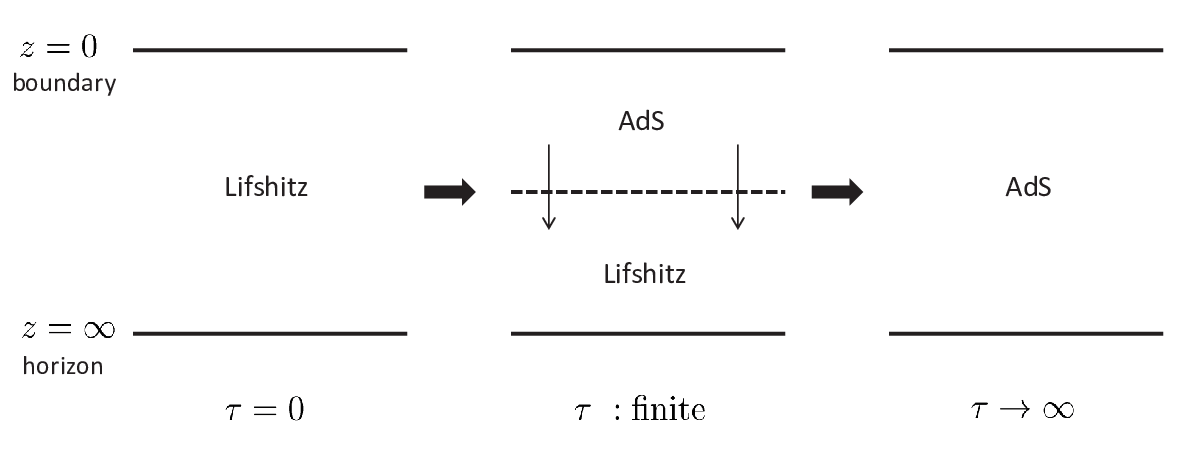
Thus the usual AdS metric has been reproduced. This implies that the Lifshitz spacetime at tends to decay to the AdS space from the boundary as . The time evolution is shown in Fig. 1. Note that the compactification radius is large enough in the near-boundary region or late time and, hence, the KK direction is effectively decompactified in the AdS region.
The next issue is to study the conformal boundary of the solutions (3.1) . It is helpful to go back to the coordinate . Then the metric is expressed as
where we have defined a new function,
Then by performing a conformal transformation for the metric as with the conformal factor,
| (3.3) |
and by taking the limit , the metric becomes
and describes a dynamical universe with a power-law expansion. It is notable that the conformal boundary is well defined, differently from the Lifshitz spacetime.
One may think that there is an external force to drive the expansion of the universe. However, the time dependence in directions comes from the time-dependent conformal factor (3.3). It makes the length scale on the boundary time dependent. This situation is described as the dynamical universe. Thus, the expansion is superficial. Indeed, the time dependence disappears by taking introduced in (3.2). Then the time-independent conformal factor leads to Minkowski spacetime, up to the dynamical S1 part.
Let us argue what happens in the boundary theory from the bulk structure. Now the AdS/CFT dictionary tells us that the short-distance physics is dominated by the bulk AdS space corresponding to equilibrium states. On the other hand, the Lifshitz spacetime influences the long-distance physics, and it may be regarded as nonequilibrium states (See Fig. 2). This means that there exists no long-range order, only ordered structure like the crystalline lattice at short distances, such as that found in the materials that exhibit the aging phenomena.
The correlation length of equilibrium state depends on time because of the expansion of the universe. The time dependence is evaluated as
| (3.4) |
where can be evaluated holographically by using the middle point value of the direction, , as in Fig. 2. This time dependence agrees with in the aging phenomena with .
Now the physical meaning of is also obvious. When , vanishes and, hence, no relaxation occurs. The whole geometry of the bulk is the Lifshitz spacetime. When , becomes infinite, and the system is completely relaxed. Then the whole bulk is the AdS space. Thus, should be identified with a typical relaxation time at microscopic scale.

Finally let us discuss the behavior of the solutions (3.1) when . There is a curvature singularity when . The location of the singularity is
| (3.5) |
and depends on time . It appears from the horizon at , and it goes up to the boundary and finally runs into the boundary at . The time evolution for is depicted in Fig. 3. In the region where , the coordinate cannot be regarded as the time direction any more. The metric in this region behaves as a Euclidean AdS (EAdS) space and the direction becomes timelike. Now that the direction is compactified, a closed timelike curve exists in this region.

The bump of the singularity may be interpreted as a quantum quench to produce nonequilibrium states. The effective time-dependent coupling , defined as
| (3.6) |
diverges rapidly as , and this may be understood as a holographic description of quantum quench [29].
In conclusion, we have shown time-dependent Lifshitz-type solutions in type IIB supergravity and discussed the time evolution in relation to the aging phenomena. It is nice to look for more general solutions corresponding to more complicated processes. A finite-temperature generalization is especially interesting.
As another aspect, our solutions give rise to a dynamical universe with a power-law expansion. This universe is not isotropic because of the KK circle expanding with time, and hence it would be difficult to construct realistic models in the present setup. It is interesting to look for other setups applicable to building the realistic model.
We hope that our results develop a new frontier for studying the time-dependent AdS/CFT correspondence and find many applications to nonequilibrium phenomena in condensed matter physics.
We would like to thank S. Nakamura for useful discussions. The work of K. Y. was supported by the scientific grants from the Ministry of Education, Culture, Sports, Science and Technology (MEXT) of Japan (No. 22740160). This work was also supported in part by the Grant-in-Aid for the Global COE Program, “The Next Generation of Physics, Spun from Universality and Emergence”, from MEXT, Japan.
References
- [1] J. M. Maldacena, Adv. Theor. Math. Phys. 2, 231 (1998).
- [2] S. S. Gubser, I. R. Klebanov and A. M. Polyakov, Phys. Lett. B 428, 105 (1998).
- [3] E. Witten, Adv. Theor. Math. Phys. 2, 253 (1998).
- [4] G. Policastro, D. T. Son and A. O. Starinets, Phys. Rev. Lett. 87, 081601 (2001).
- [5] P. Kovtun, D. T. Son and A. O. Starinets, Phys. Rev. Lett. 94, 111601 (2005).
- [6] T. Sakai and S. Sugimoto, Prog. Theor. Phys. 113, 843 (2005); Prog. Theor. Phys. 114, 1083 (2005).
- [7] S. Ryu and T. Takayanagi, Phys. Rev. Lett. 96, 181602 (2006).
- [8] S. A. Hartnoll, C. P. Herzog and G. T. Horowitz, Phys. Rev. Lett. 101, 031601 (2008).
- [9] D. T. Son, Phys. Rev. D 78, 046003 (2008).
- [10] K. Balasubramanian and J. McGreevy, Phys. Rev. Lett. 101, 061601 (2008).
- [11] S. Kachru, X. Liu and M. Mulligan, Phys. Rev. D 78, 106005 (2008).
- [12] S. A. Hartnoll, Class. Quant. Grav. 26, 224002 (2009).
- [13] J. McGreevy, Adv. High Energy Phys. 10, 723105 (2010).
- [14] S. Sachdev, Lect. Notes Phys. 828, 273 (2011).
- [15] L. C. E. Struik, Polymer Engineering and Science 17 (1977) 165.
- [16] L. F. Cugliandolo, arXiv:cond-mat/0210312.
- [17] M. Henkel and M. Pleimling, cond-mat/0703466.
- [18] For an earlier attempt for holographic aging phenomena, see D. Minic and M. Pleimling, Phys. Rev. E 78, 061108 (2008). However, their setup is invariant under time translation.
- [19] A time-dependent background is proposed as a holographic dual for the aging in J. I. Jottar, R. G. Leigh, D. Minic and L. A. Pando Zayas, J. High Energy Phys. 11 (2010) 034; S. Hyun, J. Jeong and B. S. Kim, J. High Energy Phys. 03 (2012) 010. However, the time dependence can be removed by a coordinate transformation, so the solution is essentially time independent.
- [20] G. W. Gibbons, H. Lu and C. N. Pope, Phys. Rev. Lett. 94, 131602 (2005).
- [21] W. Chen, Z. W. Chong, G. W. Gibbons, H. Lu and C. N. Pope, Nucl. Phys. B 732, 118 (2006).
- [22] H. Kodama and K. Uzawa, J. High Energy Phys. 07 (2005) 061.
- [23] W. Chemissany and J. Hartong, Class. Quant. Grav. 28, 195011 (2011).
- [24] A. Donos and J. P. Gauntlett, J. High Energy Phys. 12 (2010) 002.
- [25] K. Balasubramanian and K. Narayan, J. High Energy Phys. 08 (2010) 014.
- [26] M. Henkel, M. Pleimling, C. Godreche and J. -M. Luck, Phys. Rev. Lett. 87, 265701 (2001).
- [27] K. Copsey and R. Mann, J. High Energy Phys. 03 (2011) 039.
- [28] G. T. Horowitz and B. Way, Phys. Rev. D 85, 046008 (2012).
- [29] A holographic quantum quench is argued in another fashion in S. R. Das, T. Nishioka and T. Takayanagi, J. High Energy Phys. 07 (2010) 071; P. Basu and S. R. Das, J. High Energy Phys. 01 (2012) 103.