Inverse simulated annealing for the determination of amorphous structures
Abstract
We present a new and efficient optimization method to determine the structure of disordered systems in agreement with available experimental data. Our approach permits the application of accurate electronic structure calculations within the structure optimization. The new technique is demonstrated within density functional theory by the calculation of a model of amorphous carbon.
pacs
31.15.-p; 71.15.-m; 71.23.-k; 71.23.CqAmorphous solids can be produced from almost any chemical system and are of great interest due to their large variety of technologically important applications. In addition to conventional silicate glasses, they are, for example used in optical waveguides (oxides), plastics (organic polymers), solar cells (semiconductors), biomaterials (amorphous metals), xerography and non-volatile memory devices (chalcogenides), to name but a few [1, 2]. Nevertheless, finding their atomic scale structure is still a major challenge in material science [3, 2, 4] due to the absence of lattice periodicity and long-range order characteristics of a crystalline solid. Many sophisticated modeling techniques from the field of crystal structure prediction are based on searching the global minimum in the energy landscape for periodic structures [5, 6, 7, 8, 9, 10, 11, 12, 13]. However, an amorphous solid does not correspond to a global, but to a local energy minimum, which is energetically low enough to stabilize the structure against alternative packings and exhibits desirable target properties.
The most commonly applied computational technique to obtain the amorphous structure is to slowly quench it from the melt by Monte Carlo (MC)- or Molecular Dynamics (MD)-based Simulated Annealing (SA) [14]. However, the lack of exploitable symmetry and, therefore, large number of degrees of freedom, require the cooling to be conducted as slowly as possible to determine an approximation of the amorphous structure, and is, therefore, computationally very demanding. This is even more pronounced in conjunction with accurate ab-initio electronic structure techniques, in spite of significant progress in recent years [15, 16], allowing for satisfactory structure determinations [17, 18, 19, *CaravatiPRL, *CaravatiJPCM1, *CaravatiJPCM2, 23].
Instead of performing an elaborate calculation to obtain an approximate amorphous model and to assess a posteriori how well it matches the experiment, McGreevy and coworkers demonstrated that it can be beneficial to reverse this procedure, hence the name Reverse Monte Carlo (RMC) [24, 25]. Contrary to energy-based minimization techniques this method aims at directly modeling the structure without invoking any computationally expensive potential energy calculation, using only available experimental data. Specifically, the available experimental data are reproduced simply by minimizing a function of the form
| (1) |
under variation of the atomic positions using the Metropolis Monte Carlo method [26]. In Eq. 1, and are the calculated and experimental values, respectively, of a property , while is a weight factor and is the experimental uncertainty for the corresponding property.
Even though can, in principle, be any arbitrary property, in practice, only geometric quantities, obtainable from Neutron or X-ray scattering data such as the structure factor or the pair correlation function for which can be evaluated easily and fast, are employed. In particular, typically no electronic quantities based on accurate electronic structure calculations are utilized, which would otherwise be computationally unfeasible. While on the one hand, RMC allows for an efficient and routine modeling of rather complex disordered structures, on the other hand, the resulting models are not necessarily physically sensible. It is, therefore, good practice to circumvent that as much as possible by imposing specifically selected constraints [25, 27]. Although, eventually, this often leads to rather pleasing results, this may not be the case when studying unknown systems where good constraints are not known from the outset. In addition, since the atomic configuration in RMC is not relaxed into a local energy minimum, the resulting structure is not necessarily stable.
The inverse design technique of Franceschetti and Zunger allows one to, at least partially, circumvent the shortcomings just mentioned by determining the crystal structure based on electronic structure properties, which are rather sensitive with respect to the atomic positions. In their method, an inner local geometry optimization is performed in each optimization step to relax the structure [28]. However, for the sake of efficiency, the latter is conducted using an empirical valence force field only [29]. Furthermore, in order to facilitate the calculation, they confined themselves to highly symmetric structures on a given crystal lattice.
In this work, we improve upon the existing approaches by proposing a novel and efficient method, which we call Inverse Simulated Annealing (ISA). This method combines the global minimization of a linear combination consisting of various geometric and electronic properties with structure relaxation to determine an amorphous solid in best agreement with available experimental data. Specifically, this is achieved by adding the potential energy to the objective function of Eq. 1, and employing a modified hybrid Monte Carlo (HMC)-based SA scheme to minimize it. We will demonstrate that the present method is efficient enough to be applicable in conjunction with accurate electronic structure calculations, and in this way allows to routinely determine the amorphous structure.
In the following, we will confine ourselves to effective single-particle theories, such as density functional theory (DFT) [30]. Hence, the modified objective function to be minimized reads as:
| (2) | |||||
where is a fictitious and the potential energy, as obtained by DFT, while and are the computed and experimental values, respectively, of an electronic quantity .
In minimizing , we take advantage of the fact that by using Eq. 2, the accessible phase space is substantially reduced and restricted to energetically low-lying configurations. In other words, even though the dimensionality of the phase space is equally vast, the optimization is guided in a funnel-like fashion towards the minimum of . Obviously, in spite of that, we still need a global optimization method to minimize Eq. 2 that is efficient enough to enable the calculation of at the DFT level of theory. The fact that the derivatives of some of the properties in Eq. 2 with respect to are not directly available and may not even exist due to possible discontinuities, immediately suggests a MC-based minimization procedure [31]. The development of such a technique is therefore an essential part of the present work.
For the purpose to minimize Eq. 2, while at the same time using as few as possible electronic structure calculations, we propose here a novel ’fuzzy’ HMC-based SA scheme within the NVE instead of the more common NVT ensemble that consists of only a single modified MD step. In comparison to standard MC- or MD-based SA techniques, we found that this technique performs particularly well as a minimization method, as will be shown. The positions and velocities of all atoms in each trial move are varied according to a slightly modified velocity-Verlet algorithm:
where are the ionic velocities, the nuclear masses, a randomly chosen time step from an uniform distribution within the interval [0, ], while the prime superscripts are used to indicate quantities of the new (trial) configuration. The forces are the best possible estimate for , i.e. omitting the contributions from those terms in the sums of Eq. 2 for which no derivatives are directly available. This and the presence of a maximum time step , which is in general much larger than in standard MD and continuously adjusted to obtain an acceptance rate of about 50 %, is why we call our modified HMC algorithm ’fuzzy’. In order to ensure that the total energy is conserved, in Eq. Inverse simulated annealing for the determination of amorphous structures we have introduced an additional prefactor denoted as , which chosen in such a way that holds, where is the kinetic energy of the system of the proposed trial configuration. Within the NVE ensemble, the probability of acceptance of a trial move is given by [32]
| (6) |
where is the number of atoms.
As already mentioned, the present approach differs from the standard HMC algorithm in the fact that the NVE instead of the usual NVT ensemble is employed. Furthermore, only a single MD step is taken in each HMC step and the velocities are not randomly re-initialized thereafter. The necessary random element in our HMC method comes from the randomly chosen, variable time step instead. Whenever a HMC move is accepted, the positions and velocities are updated as , just as in normal MD. Otherwise, if an HMC move is rejected, then one possibility is to maintain , in which case no update is required. We will denote this straightforward version of our method as fHMC-NVE. However, regarding the efficiency of the minimization procedure, it is desirable to design an algorithm that combines a large time step with a high acceptance rate. It appears that an improvement in this direction is obtained by maintaining the velocities of the rejected configurations, i.e. by updating according to after a rejection. In this modified algorithm, indicated hereafter as mfHMC-NVE, the velocities are gradually turned in the direction of the forces upon repeated rejections. As a consequence, the acceptance probability for large displacements (i.e. large ) increases, since the displacements become more and more parallel to the forces, i.e. the direction of decreasing potential energy.

To assess the performance of our HMC-based minimization technique, we have applied it to carbon using the empirical LCBOPII potential [33]. This bond order potential has been shown to accurately describe many carbon phases including the disordered, liquid phase within a whole range of different densities [34]. We have selected a system consisting of 216 atoms within in a cubic simulation box with periodic boundary conditions, which corresponds to a density of g/cm3, which is in close agreement with the experimentally determined density of amorphous carbon [36]. For the sake of simplicity, in these simulations, meant to test and compare the performance of different minimization techniques, momentarily only the potential energy is minimized.
The applied total energy schedule as a function of the (fictitious) MC ’time’, is schematically shown in Fig. 1a. Starting at a high total energy eV, to create a well disordered liquid phase, the schedule includes a liquid equilibration period at constant eV, after which the system is cooled down linearly to eV during a ’time’ interval . After that, the system is relaxed in a relatively short quench by further decreasing to a value close to the final potential energy . Note that the instantaneous temperature of the system can be deduced from , which implies , so that K for .
The results for the average, final potential energy per atom at 0 K, , as a function of the cooling ’time’ interval in units of total energy evaluations (tee), based on 40 independent simulations, are shown in Fig. 1c and compared to the results from other, more standard minimization techniques. These include the reference, a random single atom displacement MC method within the NVT ensemble, indicated as RS-MC-NVT, and two all atom MC methods within the NVT ensemble: the RA-MC-NVT method with completely random, simultaneous displacements of all atoms and the FA-MC-NVT method, where the displacement of each atom is a mixture of a random vector and the force on that atom with a mixing coefficient chosen such that the efficiency is maximized. The applied temperature versus the MC ’time’ for these NVT simulations is schematically given in Fig. 1b.
As can be seen in Fig. 1c, the behavior of the RA-MC-NVT technique and the reference is essentially identically, which suggests that in the present case it is insignificant if either all or a single atom is randomly displaced. Nevertheless, the straightforward inclusion of nuclear forces in the FA-MC-NVT approach leads to an optimization scheme that can easily get trapped in a local minimum and is hence not competitive. On the contrary, in the (m)fHMC-NVE method this is circumvented by the interplay of and . On average is relatively large, i.e. typically about one order of magnitude larger than in a conventional MD simulation for carbon and remains approximately constant during the annealing. In this way, the available gradient information is rather well exploited. However, upon rejections the decrease of is counterbalanced by to conserve the instantaneous total energy and therefore prevents the system to be trapped in a local minimum. In the end, employing the mfHMC-NVE method, the same potential energy than using the RS-MC-NVT approach is realized, though with a two orders of magnitude shorter cooling time. Comparing the final potential energies with the ground state energies of diamond (-7.349 eV/atom) and graphite (-7.374 eV/atom), it is apparent that the eventual structures correspond to amorphous carbon, whose energies are about 0.4 eV/atom above the corresponding ground state.
As already mentioned, the mfHMC-NVE method shows the best performance regarding its ability to find low energy states. On the other side, it is feasible to do much longer simulations (in terms of tee) with the RS-MC-NVT method than using the other techniques, because the re-evaluation of the total energy after the displacement of one single atom is relatively fast for the empirical LCBOPII potential; this is due to the intrinsic local dependencies of the energy contributions in such potentials. Since the curve for RA-MC-NVT lies on top of that of the RS-MC-NVT technique, the latter is to be preferred whenever updating the total energy for single atom move is faster than for an all atom move.
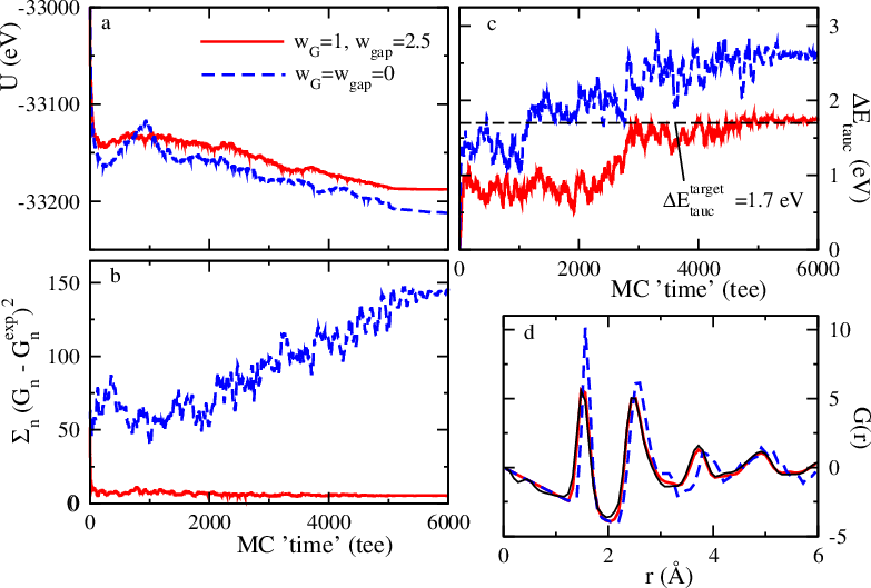
To illustrate our novel method, we apply the mfHMC-NVE method to minimize Eq. 2 for amorphous carbon at the density functional level of theory (DFT). Therein, is the total energy from DFT supplemented by the reduced radial distribution function , derived from scattering data, and the optical Tauc gap for amorphous phases [35]. Hence, in this case, Eq. 2 takes the form:
| (7) | |||||
where denotes a discretized representation of , which is defined as , with the average (number) density of atoms at a distance and the overall density. To obtain a smoothened , allowing for the calculation of analytical force contributions that were included in the present simulations, we have computed it for any on a grid with a spacing of 0.01 Å between the grid points as:
| (8) |
where is a Gaussian-shaped polynomial of degree 4 within the open interval and otherwise, with and being continuous at , and the interatomic distance between atom and . The values reported for the experimental gap of amorphous carbon vary between 1.0 eV and 2.5 eV, possibly depending on the particular sample [18]. Therefore, we have taken an intermediate target value equal to eV for our simulation. However, in the present study, we have neglected the gradient of the Tauc gap term with respect to in the analytic expression of the forces. Nevertheless, using finite differences, it is straightforward to include them, although at the price that the computation becomes at least a factor of times more expensive. Further details on the on-the-fly calculation of the Tauc gap are discussed in the Appendix.
Even though the values of the weight factors and have some importance, their impact is relatively small. In principle they should be chosen as small as possible and just large enough to get a good agreement with the experimental data. In the present simulation we have used and . In general, the value should be chosen in such a way that, in the beginning of the simulation at high temperature, is on the same order of magnitude than the thermal energy . In contrast, the parameter can be selected to be considerable smaller than .
We have linked our code to the CP2K suite of programs to compute the necessary total energies and forces [37]. The DFT calculations were performed using the Perdew-Burke-Ernzerhof (PBE) exchange correlation functional [38] and norm-conserving Goedecker-type pseudopotentials [39]. The total energy schedule applied included an equilibration at eV for 1000 tee, followed by a cooling from eV to eV during 4000 tee and a final run of length 1000 tee during which is further lowered to get as close as possible to .
The results of such simulations using our novel method, with and without the experimental constraints, are presented in Fig. 2 and are compared to a conventional HMC-based SA simulation. The improved overall agreement with the underlying experimental data is apparent, as shown in Figs. 2c and 2d.
We conclude by noting that our novel method in conjunction with an appropriate minimization procedure has a wide domain of applicability, not limited to amorphous phases. We wish to specifically highlight that the present scheme can be directly applied to any other disordered system, such as liquid water [40, *Kuehne2011, *PascalWater, *Kuehne2013] or, including the NMR chemical shift [44, *MauriNMR2, 46, *SebastianiParrinelloWaterNMR], to determine the structure of proteins and nucleic acids. Further improvement of the method and the minimizer will be presented elsewhere.
Acknowledgements.
We would like to thank A. Zunger for fruitful discussions, D. Richters for critical reading the manuscript as well as the IDEE project of the Carl-Zeiss Foundation and the Graduate School of Excellence MAINZ for financial support.I Appendix: Tauc gap
The optical Tauc gap is a convenient definition for the gap of amorphous phases, which circumvents the difficulty that the band structure of disordered systems is not properly defined. It relies on the following relation [35] between the experimental optical gap and the optical absorption coefficient as a function of the photon energy :
| (9) |
which is applicable to (amorphous) semi-conductors within a certain range of photon energies just beyond the gap . For the on-the-fly calculation of within each optimization step, we first compute the optical absorption coefficient from [48]:
| (10) |
where is a constant, while and are the densities of the occupied and unoccupied states that are computed from the eigenvalue spectrum of the DFT Hamiltonian after self-consistency has been achieved. Plotting as a function of within a photon energy range around the gap obeys a linear regime, from which can be obtained by taking the intersection between the linear fit with the horizontal axis. We note that the value of the constant is irrelevant for the value of resulting from this approach. Since the linear behavior only applies to a finite energy range just beyond the gap, the linear fit has to be restricted to this energy interval. For the automatic computation of , we have selected this interval to be within the interval , where is the total width of the spectrum.
References
- [1] R. Zallen, The Physics of Amorphous Solids, Wiley, New York, 1983.
- [2] S. R. Elliott, Physics of Amorphous Materials, Longman Scientific & Technical, Essex, 1990.
- [3] W. H. Zachariasen, J. Am. Chem. Soc. 54, 3841 (1932).
- [4] M. Jansen, J. C. Schön and L. van Wüllen, Angew. Chem. Int. Ed. 45, 4244 (2006).
- [5] J. Maddox, Nature 335, 6187 (1988).
- [6] D. M. Deaven and K. M. Ho, Phys. Rev. Lett. 75, 288 (1995).
- [7] D. J. Wales and H. A. Scheraga, Science 285, 1368 (1999).
- [8] R. Martonak, A. Laio and M. Parrinello, Phys. Rev. Lett. 90, 075503 (2003).
- [9] S. Goedecker, J. Chem. Phys. 120, 9911 (2004).
- [10] C. W. Glass, A. G. Oganov and N. Hansen, Comp. Phys. Commun. 175, 713 (2006).
- [11] G. Trimarchi and A. Zunger, Phys. Rev. B 75, 104113 (2007).
- [12] S. C. Woodley and R. Catlow, Nature Mater. 7, 937 (2008).
- [13] C. Wehmeyer, G. F. von Rudorff, S. Wolf, G. Kabbe, D. Schärf, T. D. Kühne and D. Sebastiani, J. Chem. Phys. 137, 194110 (2012).
- [14] S. Kirkpatrick, C. D. Gelatt, M. P. Vecchi, Science 220, 671 (1983).
- [15] R. Car and M. Parrinello, Phys. Rev. Lett. 55, 2471 (1985).
- [16] T. D. Kühne, M. Krack, F. R. Mohamed and M. Parrinello, Phys. Rev. Lett. 98, 066401 (2007).
- [17] J. Sarnthein, A. Pasquarello and R. Car, Phys. Rev. Lett. 74, 4682 (2005); Phys. Rev. B 52, 12690 (1995).
- [18] N. A. Marks, D. R. McKenzie, B. A. Pailthorpe, M. Bernasconi and M. Parrinello, Phys. Rev. Lett. 76, 768 (1996); Phys. Rev. B 54, 9703 (1996).
- [19] S. Caravati, M. Bernasconi, T. D. Kühne, M. Krack and M. Parrinello, Appl. Phys. Lett. 91, 171906 (2007).
- [20] S. Caravati, M. Bernasconi, T. D. Kühne, M. Krack and M. Parrinello, Phys. Rev. Lett. 102, 205502 (2009).
- [21] S. Caravati, M. Bernasconi, T.D. Kühne, M. Krack and M. Parrinello, J. Phys.: Condens. Matter 21, 255501 (2009).
- [22] S. Caravati, D. Colleoni, R. Mazzarello, T. D. Kühne, M. Krack, M. Bernasconi and M. Parrinello, J. Phys.: Condens. Matter 23, 265801 (2011).
- [23] M. F. Camellone, T. D. Kühne and D. Passerone, Phys. Rev. B 80, 033203 (2009).
- [24] R. L. McGreevy and L. Pusztai, Mol. Simul. 1, 359 (1988).
- [25] R. L. McGreevy, J. Phys.: Condens. Matter 13, R877 (2001).
- [26] N. Metropolis, A. W. Rosenbluth, M. N. Rosenbluth, A. H. Teller and E. Teller, J. Chem. Phys. 21, 1087 (1953).
- [27] S. Kugler, L. Pusztai, L. Rosta, P. Chieux and R. Bellissent, Phys. Rev B 48, 7685 (1993).
- [28] A. Franceschetti and A. Zunger, Nature 401, 60 (1999).
- [29] P. N. Keating, Phys. Rev. B 149, 674 (1966).
- [30] R. O. Jones and O. Gunnarsson, Rev. Mod. Phys. 61, 689 (1989).
- [31] S. Duane, A. D. Kennedy, B. J. Pendleton and D. Roweth, Phys. Lett. B 2, 216 (1987).
- [32] J. R. Ray, Phys. Rev. A 44, 4061 (1991).
- [33] J. H. Los, L. M. Ghiringhelli, E. J. Meijer and A. Fasolino, Phys. Rev. B 72, 214102 (2005).
- [34] L. M. Ghiringhelli, J. H. Los, A. Fasolino and E. J. Meijer, Phys. Rev. B 72, 214103 (2005).
- [35] J. Tauc, A. Menth and D. L. Wood, Phys. Rev. Lett. 25, 749 (1970).
- [36] W. R. Gilkes, P. H. Gaskell, and J. Robertson, Phys. Rev. B 51, 12303 (1995).
- [37] J. VandeVondele, M. Krack, F. Mohamed, M. Parrinello, T. Chassaing and J. Hutter, Comput. Phys. Commun. 167, 103 (2005).
- [38] J. P. Perdew, K. Burke and M. Ernzerhof, Phys. Rev. Lett. 77, 3865 (1996).
- [39] S. Goedecker, M. Teter and J. Hutter, Phys. Rev. B 54, 1703 (1996).
- [40] T. D. Kühne, M. Krack and M. Parrinello, J. Chem. Theory Comput. 5, 235 (2009).
- [41] T. D. Kühne, T. A. Pascal, E. Kaxiras and Y. Jung, J. Phys. Chem. Lett. 2, 105 (2011).
- [42] T. A. Pascal, D. Schärf, Y. Jung and T. D. Kühne, J. Chem. Phys. 137, 244507 (2012).
- [43] T. D. Kühne and R. Z. Khaliullin, Nature Commun. 4, 1450 (2013).
- [44] F. Mauri, B. G. Pfrommer and S. G. Louie, Phys. Rev. Lett. 77, 5300 (1996).
- [45] F. Mauri, B. G. Pfrommer and S. G. Louie, Phys. Rev. Lett. 79, 2340 (1997).
- [46] D. Sebastiani and M. Parrinello, J. Phys. Chem. A 105, 1951 (2001).
- [47] D. Sebastiani and M. Parrinello, Phys. Chem. Chem. Phys. 3, 675 (2002).
- [48] R. Bouzerar, C. Amory, A. Zeinert, M. Benlahsen, B. Racine, O. Durand-Drouhin and M. Clin, Journal of Non-Crystalline Solids 281, 171 (2001).