Bar 1-Visibility Drawings of 1-Planar Graphs
Abstract
A bar -visibility drawing of a graph is a drawing of where each vertex is drawn as a horizontal line segment called a bar, each edge is drawn as a vertical line segment where the vertical line segment representing an edge must connect the horizontal line segments representing the end vertices and a vertical line segment corresponding to an edge intersects at most one bar which is not an end point of the edge. A graph is bar 1-visible if has a bar 1-visibility drawing. A graph is 1-planar if has a drawing in a 2-dimensional plane such that an edge crosses at most one other edge. In this paper we give linear-time algorithms to find bar 1-visibility drawings of diagonal grid graphs and maximal outer 1-planar graphs. We also show that recursive quadrangle 1-planar graphs and pseudo double wheel 1-planar graphs are bar -visible graphs.
1 Introduction
A -planar drawing of a graph is a drawing of on a two dimensional plane where an edge can be crossed by at most another edge. A graph is -planar if has a 1-planar drawing. A straight-line drawing of a graph is a drawing of such that every edge of is drawn as a straight-line segment. A right angle crossing drawing or RAC drawing is a straight-line drawing where any two crossing edges form right angles at their intersection point. A RAC graph is a graph that has a RAC drawing. A bar -visibility drawing of a graph is a drawing of where each vertex is drawn as a horizontal line segment called a bar, each edge is drawn as a vertical line segment where the vertical line segment representing an edge must connect the horizontal line segments representing the end vertices and a vertical line segment corresponding to an edge intersects at most one bar which is not an end point of the edge. A graph is a bar -visible if has a bar 1-visibility drawing. A bar -visible graph and a bar -visibility drawing of the same graph is shown in Figures 1 (a), and (b), respectively.

Recently 1-planar graphs and RAC graphs have been extensively studied [2, 8, 10, 16]. Pach and Toth proved that 1-planar graphs with vertices have at most edges [14], whereas Didimo et al. showed that a RAC graph with vertices has at most edges [7]. Recognizing the both classes of graphs are NP-hard [1, 11]. Recently Eades and Liotta studied the relationship between dense RAC graphs and dense 1-planar graphs [9].
The concept of bar visibility drawing came up in the early 1980s when many new problems in visibility theory arose, originally inspired by applications dealing with determining visibilities between different electrical components in VLSI design. Other applications arise when large graphs are to be displayed in a transparent way, and in the rapidly developing field of computer graphics. A bar visibility drawing of a planar graph is a drawing of where each vertex is drawn as a horizontal line segment and each edge is drawn as a vertical line segment where the vertical line segment representing an edge must connect the horizontal line segments representing the end vertices. Otten and Wijk [13] have shown that every planar graph admits a visibility drawing, and Tamassia and Tollis [17] have given a linear-time algorithm for constructing a visibility drawing of a planar graph. Dean et al. have introduced a generalization of visibility drawing for a non-planar graph which is called bar -visibility drawing [4]. In a bar -visibility drawing of a graph a horizontal line corresponding to a vertex is called a bar, and the vertical line segment corresponding to an edge intersects at most bars which are not end points of the edge. Thus a visibility drawing is a bar -visibility drawing for .
In this paper we give linear-time algorithms to find bar 1-visibility drawings of diagonal grid graphs and maximal outer 1-plane graphs which are RAC drawable graphs. We also develop algorithms for finding bar 1-visibility drawings of recursive quadrangle 1-planar graphs and pseudo double wheel 1-planar graphs which are not RAC graphs.
The rest of the paper is organized as follows. Section 2 describes some of the definitions that we have used in our paper. Sections 3 deals with linear algorithms for finding bar 1-visibility drawings of diagonal grid graphs and maximal outer 1-plane graphs and Section 4 deals with algorithms for finding bar 1-visibility drawings of recursive quadrangle 1-planar graphs and pseudo double wheel 1-planar graphs. Finally, Section 5 concludes our paper with a list of open problems.
2 Preliminaries
In this section we introduce some terminologies and definitions which will be used throughout the paper. For the graph theoretic definitions which have not been described here, see [6, 12].
A graph is planar if it can be embedded in the plane without edge crossing except at the vertices where the edges are incident. A plane graph is a planar graph with a fixed planar embedding. A plane graph divides the plane into some connected regions called the faces. The unbounded region is called the outer face and all the other faces are called the inner faces. The vertices on the outer face are called the outer vertices and all the other vertices are called inner vertices.
A -grid graph is a graph whose vertices correspond to the grid points of a -grid in the plane and edges correspond to the grid lines between two consecutive grid points. A diagonal grid graph is a -grid graph with diagonal edges are introduced in each cell. Figure 2(a) shows a -grid graph and Figure 2(b) shows a diagonal grid graph . Let be a cell of a diagonal grid graph as illustrated in Figure 2(c), where is the bottom-left vertex, is the bottom-right vertex, is the up-right vertex and is the up-left vertex. We call the edge the right-diagonal edge and the edge the left-diagonal edge of the cell .

An acyclic digraph with a single source and a single sink is called an -graph. A plane -graph is an -graph that is planar and embedded with vertices and on the boundary of the outer face. Let be a plane -graph and be its set of faces. contains two representatives of the outer face: the ”left outer face” , which is incident with the edges on the left boundary of and the ”right outer face” , which is incident with the edges on the right boundary of . Additionally, for each we define and . Also, we define (respectively ) to be the face to the left (respectively right) of . We now define a dual-like graph of as follows. The vertex set of is the set of faces of , and has an edge for each edge of , where and . In Figure 2(d) the vertices and edges of are drawn by black circles and solid lines respectively, and the vertices and edges of are drawn by white rectangles and dotted lines respectively.
Let be a digraph with vertices and edges. A topological numbering of is an assignment of numbers to the vertices of , such that, for every edge of , the number assigned to is greater than the one assigned to . If the edges of digraph have nonnegative weights associated with them, a weighted topological numbering is a topological numbering of , such that, for every edge of , the number assigned to is greater than or equal to the number assigned to plus the weight of . The numbering is optimal if the range of numbers assigned to the vertices is minimized.
Let be a planar -graph with vertices. Two paths and of are said to be non-intersecting if they are edge disjoint and do not cross at common vertices but they can touch at vertices. Let be a collection of non-intersecting paths of . In the visibility drawing of , for every path of , if the edges of are vertically aligned then the drawing is called constrained visibility drawing. The following result on constrained visibility drawing is known [3].
Lemma 1
Let be a planar -graph with vertices, and let be a set of non-intersecting paths of . Then one can find a constrained visibility drawing of in time with area, where the edges of every path in are vertically aligned.
A -planar drawing of a graph is a drawing of on a two dimensional plane where an edge can be crossed by at most another edge. A graph is -planar if has a 1-planar drawing. A 1-planar graph is optimal if no edges can be added to without losing 1-planarity. That is, an optimal 1-planar graph of vertices has the highest number of edges among all 1-planar graphs of vertices. An outer-1-plane graph is a topological embedding of a graph such that all vertices lie on the outer face and there is at most one crossing on each edge. An outer-1-plane graph is a maximal outer-1-plane graph if for each pair of vertices where is not an edge, adding the edge to makes it not outer-1-plane; that is, is not outer-1-plane for every drawing of the edge .
3 Bar 1-Visibility Drawings of 1-Planar RAC Graphs
Some interesting labeling properties of diagonal grid graphs have been studied recently by Selvaraju and Pricilla [15]. Recently Dehkordi showed that outer-1-plane graphs are RAC graphs [5]. In this section we give linear-time algorithms for finding bar 1-visibility drawings of diagonal grid graphs and maximal outer 1-plane graphs which are RAC drawable graphs. In Section 3.1 we develop an algorithm for finding a bar 1-visibility drawing of a diagonal grid graph and in Section 3.2 we develop an algorithm for finding a bar 1-visibility drawing of a maximal outer 1-plane graph.
3.1 Diagonal Grid Graphs
In this Section we prove the following theorem.
Theorem 3.1
A bar 1-visibility drawing of a diagonal grid graph can be drawn in linear-time.
Proof
Let be a diagonal grid graph as illustrated in Figure 3(a). Clearly is RAC drawable and 1-planar. We will prove that is bar 1-visible by constructing a bar 1-visibility drawing of . We first obtain a graph from by deleting the left-diagonal edge of each cell. Clearly is a plane graph as illustrated in Figure 3(b). Let , and , be the vertex corresponding to the grid point on the th row and th column of the grid. We now assign a number to each vertex as follows. We set for , and for we set . We now construct a directed graph from by assigning direction to each edge from lower number to higher number. We add a vertex below the first row and a vertex above the last row. We also add directed edges and for . Let be the resulting digraph as illustrated in Figure 3(c). From the construction one can observe that is an -graph. We now construct a visibility drawing of as follows [17].
We first construct of and assign unit weights to the edges of and compute an optimal weighted topological numbering of as illustrated in Figure 3(d). We then draw each vertex as a horizontal line segment at -coordinate and between -coordinate and . We call the start of and the end of . For each edge , we draw the vertical line segment at -coordinate , between -coordinate and . Let be the upper-left vertex and be the bottom-right vertex of a cell in a diagonal grid graph. Then one can observe from the drawing algorithm that .
We now obtain a bar 1-visibility drawing of from the visibility drawing of as follows. We first delete and from the drawing together with the drawings of the edges incident to and . The visibility drawing of is illustrated in Figure 3(e). We insert one vertical grid line (column) between the two consecutive vertical grid lines and if and for some right diagonal edge by expanding the drawing towards direction. We perform this insertion operation for every . After this insertion operation the difference of -coordinate of end of and start of will be three, where is the upper-left vertex and is the bottom-right vertex of a cell in a diagonal grid graph. We thus extend the end of by 2 unit in -direction and the end of by one unit to the -direction. We can place the deleted left diagonal edges in the vertical segment which will be placed between starting point of the horizontal bar corresponding to bottom-right vertex and end point of the extended horizontal segment corresponding to up-left vertex in each cell. By extending these bars, the right diagonal edge in each cell crosses horizontal bar corresponding to up-left vertex in the drawing. Since all edges including left diagonal edges can be placed at end point and start point of the horizontal bars then only right diagonal edges always pass through one horizontal bar corresponding to the vertex, the drawing becomes a bar 1-visibility drawing. The bar 1-visibility drawing of is illustrated in Figure 3(f).

Theorem 3.2
A diagonal grid graph admits a bar -visibility drawing on a grid of size . Furthermore, can be found in linear-time.
Proof
Let be a diagonal grid graph. We first obtain a graph from by deleting the left-diagonal edge of each cell. Then according to proof of theorem 1, we can get visibility drawing of the graph . The height of the drawing is . The width of the drawing is the length of the longest path in . Since each cell of contains two faces, the longest path of is at most . We now compute the size of bar 1-visibility drawing. One can observe that at most new columns are inserted for constructing bar 1-visibility drawing of from the visibility drawing of . Thus the width of the bar 1-visibility drawing is . Thus we can obtain a bar -visibility drawing on a grid of size .
A diagonal grid graph has vertices. If then the area of the bar 1-visibility drawing is and if then the area is . When then the area of the bar -visibility drawing is . The bar 1-visibility drawing obtained by our algorithm is “compact” in a sense that there is at least one line segment for every vertical and horizontal grid line except the last vertical grid line.
3.2 Maximal Outer 1-Planar Graphs
In this Section we give an algorithm for obtaining a bar 1-visibility drawing of a maximal outer 1-plane graph. This problem has an interesting correlation with a constrained visibility drawing of a planar -graph. To describe the algorithm, we have need some definitions.
Let be a maximal outer 1-plane graph. In a maximal outer 1-plane graph, each edge crossing is surrounded by a cycle of length 4 and no edge in this cycle has a crossing [5]. We call such a cycle of length four a quadrangle. An edge of an outer-1-plane graph is called a crossing edge if has a crossing; otherwise is called a non-crossing edge. In the Figure 4(a), and are quadrangles. In quadrangle , edges and are crossing edges and edges , , , are non-crossing edges. The crossing edges of a quadrangle are called diagonal of the quadrangle.
We call a labeling of vertices of a maximal outer 1-plane graph by integers 1 to (where is the number of vertices in the graph) a diagonal labeling if vertices of each quadrangle got numbers in such a way that two ends of a diagonal of a quadrangle get the lowest and highest numbers among the numbers assigned to the four vertices of the quadrangle.
For example, Figure 4(a) shows an input maximal outer 1-plane graph and Figure 4(b) shows a diagonal labeling of .
We can introduce diagonal labeling on the maximal outer 1-plane graph. We have the following lemma.
Lemma 2
Every maximal outer 1-plane graph admits diagonal labeling.
Proof
Let be a maximal outer 1-plane graph. We will prove that has a diagonal labeling. Let be a vertex in . Then assign 1 to . After that we will give next numbers to those vertices which are incident to non-crossing edges from in counterclockwise order. Then assign numbers to the vertices which are incident to crossing edges from . We then consider the vertex labeled by 2 and assign next numbers to the vertices in the same way. Since the labeling has done always in increasing order and the vertices incident to crossing edges are labeled later, so the diagonal of a quadrangle got the highest and lowest numbers among the numbers of four vertices of the quadrangle. Figure 4(b) illustrates a diagonal labeling of the maximal outer 1-plane graph in Figure 4(a).
Using this diagonal labeling, we can construct a bar 1-visibility drawing of a maximal outer 1-plane graph as mentioned in the following theorem.
Theorem 3.3
A bar 1-visibility drawing of a maximal outer 1-plane graph can be drawn in linear-time.
Proof
Let be a maximal outer 1-plane graph as illustrated in Figure 4(a). By Lemma 2, has a diagonal labeling as illustrated in Figure 4(b). We first give direction to every edge from lower number to higher number as illustrated in Figure 4(b). We next identify the crossing edge containing the highest number and the lowest number in each quadrangle. We next construct a planar graph from by passing the crossing edge containing the highest number and the lowest number through the vertex which are right side of the edge in each quadrangle as illustrated in Figure 4(c). The crossing edge which is passed through the vertex is identified as a non-intersecting path. Since we pass all the crossing edges through the vertices which are right side of the edges, these satisfies the conditions of non-intersecting paths stated in the result on constrained visibility drawing [3]. In the graph illustrated in Figure 4(c), more than one sink vertices are found. We next construct planar -graph by adding dummy edges between the sink vertices to the highest labeled sink vertex as illustrated in Figure 4(d). Since the graph is outer planar, the obtained graph remains planar after adding dummy edges. We next construct a constrained visibility drawing of this planar -graph according to Lemma 1 [3]. All edges can be placed at end point and start point of the horizontal bars. Since crossing edges containing the highest number and the lowest number for all quadrangles always pass through one horizontal bar corresponding to the vertex, the drawing becomes a bar 1-visibility drawing. Since every step of the algorithm can be done in linear-time, a bar 1-visibility drawing of a maximal outer 1-plane graph can be drawn in linear-time [3]. The bar 1-visibility drawing of is illustrated in Figure 4(e).

4 Bar 1-Visibility Drawings of 1-Planar Non-RAC Graphs
In the previous section, we showed that diagonal grid graphs and maximal outer 1-planar graphs are two classes of 1-planar graphs. Recently Eades and Liotta showed that every maximally dense RAC graph is 1-planar [9]; on the other hand, they introduced a class of 1-planar graphs which is not RAC drawable. In this section we call the class recursive quadrangle 1-planar graphs. Suzuki studied the combinatorial properties of the optimal 1-planar graphs having edges [16] which we will define as “pseudo double wheel 1-planar graphs”. Since a RAC graph with vertices has at most edges [7], pseudo double wheel 1-planar graphs are not RAC graphs. In this section we show that recursive quadrangle 1-planar graphs and pseudo double wheel 1-planar graphs are bar 1-visible graphs. In Section 4.1 we develop an algorithm for finding a bar 1-visibility drawing of a recursive quadrangle 1-planar graph and in Section 4.2 we develop an algorithm for finding a bar 1-visibility drawing of a pseudo double wheel 1-planar graph.
4.1 Recursive Quadrangle 1-Planar Graphs
The class recursive quadrangle 1-planar graph is defined recursively, as follows. is a 1-planar graph of eight vertices . has an 1-planar drawing as illustrated in Figure 5(a) where the cycle is drawn as the outer rectangle and none of the four edges on the outer rectangle has a crossing. Let be the outer rectangle of , . Graph is obtained from by adding a new outer rectangle and 16 new edges as described in Figure 5(c) and (e), where the four edges on the the outer face do not have any crossing.
Let be a 1-planar graph and be a vertex of and be an edge of . We denote by , a bar 1-visibility drawing of , the drawing of a vertex as a horizontal bar in , and the drawing of a an edge as a vertical line segment in , respectively. For a vertex in , let and be the -coordinates of the two ends of such that . We call and the left end and the right end of , respectively. We now have the following theorem.
Theorem 4.1
Every recursive quadrangle 1-planar graph is a bar 1-visible graph.
Proof
We prove the claim by induction on . Let be the outer rectangle of , as illustrated in Figure 5(a). Then has a bar 1-visibility drawing, as illustrated in Figure 5(b) where (i) is the bottommost bar, is the topmost bar, is the second bottommost bar and is the second topmost bar; (ii) starts of and have the smallest -coordinate of the drawing and starts of and have the second smallest -coordinate of the drawing; and (iii) crosses . We assume that and , for , has a bar visibility drawing satisfying (i)-(iii) above. We now show that has a bar 1-visibility drawing satisfying (i)-(iii) above. Let be the outer rectangle of . We obtain a graph by deleting the four vertices on the outer rectangle of . Let be the outer rectangle of . By induction hypothesis, has a bar 1-visibility drawing satisfying (i)-(iii) as illustrated in Figure 5(d). We now obtain a bar 1-visibility drawing of from the visibility drawing of as follows. Extend the left ends of , and by four, four and two units, respectively, to the -direction. Extend the right ends of and by five unit each to the -direction. Draw and as the bottommost, 2nd bottommost, 2nd topmost and topmost bars outside and draw the new edges as vertical line segments such that (i)-(iii) are satisfied in , as illustrated in Fig. 5(f).

By adding two more edges to recursive quadrangle 1-planar graph of , vertices, we can obtain an optimal 1-planar graph of , vertices. From the bar 1-visibility drawing of we can obtain a bar 1-visibility drawing of by adding the drawing of additional two edges as vertical line segment, as illustrated in Figure 6. Thus the following theorem holds.
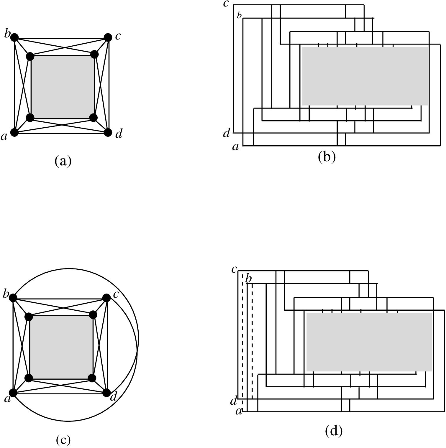
Theorem 4.2
Every optimal 1-planar graph obtained from recursive quadrangle 1-planar graph by adding two edges is a bar 1-visible graph.
4.2 Pseudo Double Wheel 1-Planar Graphs
Let be a cycle … of even number of vertices embedded on a plane. Let and be two vertices outside and inside of , respectively. We add with and with for . Let be the resulting plane graph, as illustrated in Figure 7(a). We add a pair of crossing edges to each face of , as illustrated in Figure 7(b). The resulting graph is an optimal 1-planar graph as introduced by Suzuki [16]. We call this optimal 1-planar graph even pseudo double wheel 1-planar graph.

splitting is an expansion operation at defined as follows : (i) Identify and such that there are and edges but no edge. (ii) Split path (iii) Rename one copy of as . (iv) Join , and , . Splitting is illustrated in Figure 7(d). An optimal 1-planar graph obtained from even pseudo double wheel 1-planar graph by one splitting operation is called odd pseudo double wheel 1-planar graph as illustrated in Figure 7(c). We now have the following theorem.
Theorem 4.3
Every pseudo double wheel 1-planar graph is a bar 1-visible graph.
Proof
We will prove every even pseudo double wheel 1-planar graph and odd pseudo double wheel 1-planar graph is a bar 1-visible graph.
Let be an even pseudo double wheel 1-planar graph. We will prove that is a bar 1-visible graph by constructing a bar 1-visibility drawing of . We first draw bars where topmost bar is , topmost bar is and other n-2 bars starting from topmost bar are , , , …, respectively. We next draw vertical lines from , , , …, to each crossing and another vertical lines from , , , …, to without crossing any bar. We next join each of the , , , …, bars to 4 bars 1 and 2 unit up and below itself. We next consider , , and . We next join to , to , to and to by vertical lines without crossing any bar. At last we draw a vertical line from to crossing . Since each vertical line crosses at most one bar, the drawing becomes bar 1-visibility drawing. The bar 1-visibility drawing of is illustrated in Figure 8(a).
Let be an odd pseudo double wheel 1-planar graph of vertices. We will prove that is a bar 1-visible graph by constructing a bar 1-visibility drawing of . We first find and on C such that and have degree 8. We next draw bars where 1st topmost bar is , 2nd topmost bar is , 3rd topmost bar is and other bars starting from 4th topmost bar are , , , …, respectively. We next draw vertical lines from , , , …, to without crossing any bar. Then join to ,, , … by vertical lines. These lines cross bar . We next draw vertical lines from to ,, , …, , , … crossing bar . We next join each of the , , , …, bars to 4 bars 1 and 2 unit up and below itself. Now we consider , , and . We next join to , to , to and to , to by vertical lines without crossing any bar. We next draw a vertical line from to crossing . At last we join to . Since each vertical line crosses at most one bar, the drawing becomes bar 1-visibility drawing. The bar 1-visibility drawing of is illustrated in Figure 8(b).

5 Conclusion
In this paper we give linear-time algorithms to find bar 1-visibility drawings of diagonal grid graphs and maximal outer 1-planar graphs which are RAC drawable graphs. We also developed algorithms for finding bar 1-visibility drawings of recursive quadrangle 1-planar graphs and pseudo double wheel 1-planar graphs which are not RAC drawable graphs.
Pach and Toth [14] proved that a 1-planar graph can have at most edges whereas Dean et al. [4] showed that a bar 1-visible graph can have at most edges. The bound for bar 1-visible graph is tight since for each there exists a bar 1-visible graph with exactly edges [4]. Thus not all bar 1-visible graphs are 1-planar graphs. This can be well illustrated by the following example. A bar 1-visibility drawing of an optimal 1-planar graph of eight vertices in Figure 9(a), is shown in Figure 9(b), but Figure 9(c) shows a bar 1-visibility drawing of a graph of eight vertices which has more edges. Suzuki [16] proved that every optimal 1-planar graph can be obtained from a even pseudo double wheel 1-planar graph by a sequence of splittings and “ additions”. We were able to construct bar 1-visibility drawing of every 1-planar graph that we considered as an example, but yet to find a formal proof. We thus conjecture as follows.

Conjecture 1
Every 1-planar graph is a bar 1-visible graph.
Several interesting open problems have come out from this works.
- 1.
Recognition of both RAC graphs and 1-planar graphs are NP-complete problems. It is interesting to know the complexity of recognizing a bar 1-visible graph. Finding a complete characterization of bar 1-visible graph is also an interesting open problem.
- 2.
How to find a 1-planar embedding of a 1-planar graph?
- 3.
Can we find a complete characterization of bar -visibility drawing?
References
- [1] Argyriou, E.N., Bekos, M.A., Symvonis, S.: The straight-line rac drawing problem is NP-hard. In: The Proceedings of SOFSEM’11. Lecture Notes in Computer Science, vol. 6543, p. 74–85. Springer-Verlag (2011)
- [2] Arikushi, K., Fulek, R., Keszegh, B., Moric, F., Tóth, C.D.: Graphs that admits right angle crossing drawing. In: The Proceedings of WG’10. Lecture Notes in Computer Science, vol. 6410, p. 135–146. Springer-Verlag (2010)
- [3] Battista, D., Tamassia, R., Tollis, I.G.: Constrained visibility representation of graphs. In: Inform. Process. Letters. vol. 41, pp. 1–7 (1992)
- [4] Dean, A.M., Evans, W., Gethner, E., Laison, J.D., Safari, M.: Bar k-Visibility Graphs. Journal of Graph Algorithms and Applications 11(1), 45–59 (2007)
- [5] Dehkordi, H.R.: On Algorithmic Right Angle Crossing Graph Drawing. Thesis, MPhil, The University of Sydney (August, 2012)
- [6] Di Battista, G., Eades, P., Tamassia, R., Tollis, I.G.: Graph Drawing: Algorithms for the Visualization of Graphs. Prentice-Hall Inc. (1999)
- [7] Didimo, W., Eades, P., Liotta, G.: Drawing graphs with right angle crossings. In: The Proceedings of WADS’09. Lecture Notes in Computer Science, vol. 5664, p. 206–217. Springer-Verlag (2009)
- [8] Didimo, W., Eades, P., Liotta, G.: A characterization of complete bipartite rac graphs. Information Processiong Letters 110(16), 687–691 (2010)
- [9] Eades, P., Liotta, G.: Right angle crossing graphs and 1-planarity. In: The Proceedings of Graph Drawing’11. Lecture Notes in Computer Science, vol. 7034, p. 206–217. Springer-Verlag (2012)
- [10] Fabrici, I., Madaras, T.: The structure of 1-planar graphs. Discrete Mathematics 307(7-8), 854–865 (2007)
- [11] Korzhik, V.P., Mohar, B.: Minimal obstructions for 1-immersions and hardness of 1-planarity testing. In: The Proceedings of Graph Drawing’08. Lecture Notes in Computer Science, vol. 5417, p. 302–312. Springer-Verlag (2008)
- [12] Nishizeki, T., Rahman, M.S.: Planar Graph Drawing. Lecture notes series on computing, World Scientific (2004)
- [13] Otten, J., Wijk, J.G.V.: Graph Representation in Interactive Layout Design. In: The Proceedings of IEEE Intternational Symposium On Circuits and Systems. pp. 914–918 (1978)
- [14] Pach, J., Tóth, G.: Graphs drawn with few crossings per edge. Combinatorica 17(3), 427–439 (1997)
- [15] Selvaraju, P., Pricilla, B.: On Cordial Labeling: The Grid, Diagonal Grid, Structured Web Graphs. International Journal of Algorithms, Computing and Mathematics 2(1), 5–14 (2009)
- [16] Suzuki, Y.: Optimal 1-planar graphs which triangulate other surfaces. Discrete Mathematics 310(1), 6–11 (2010)
- [17] Tamassia, R., Tollis, I.G.: A Unified Approach to Visibility Representations of Planar Graphs. Discrete and Computational geometry 1, 321–341 (1986)