Finite-time Consensus for Multi-agent Networks with Unknown Inherent Nonlinear Dynamics
Abstract
This paper focuses on analyzing the finite-time convergence of a nonlinear consensus algorithm for multi-agent networks with unknown inherent nonlinear dynamics. Due to the existence of the unknown inherent nonlinear dynamics, the stability analysis and the finite-time convergence analysis of the closed-loop system under the proposed consensus algorithm are more challenging than those under the well-studied consensus algorithms for known linear systems. For this purpose, we propose a novel stability tool based on a generalized comparison lemma. With the aid of the novel stability tool, it is shown that the proposed nonlinear consensus algorithm can guarantee finite-time convergence if the directed switching interaction graph has a directed spanning tree at each time interval. Specifically, the finite-time convergence is shown by comparing the closed-loop system under the proposed consensus algorithm with some well-designed closed-loop system whose stability properties are easier to obtain. Moreover, the stability and the finite-time convergence of the closed-loop system using the proposed consensus algorithm under a (general) directed switching interaction graph can even be guaranteed by the stability and the finite-time convergence of some special well-designed nonlinear closed-loop system under some special directed switching interaction graph, where each agent has at most one neighbor whose state is either the maximum of those states that are smaller than its own state or the minimum of those states that are larger than its own state. This provides a stimulating example for the potential applications of the proposed novel stability tool in the stability analysis of linear/nonlinear closed-loop systems by making use of known results in linear/nonlinear systems. For illustration of the theoretical result, we provide a simulation example.
Index Terms:
Consensus, Cooperative Control, Nonlinear Dynamics, Multi-agent Systems, Finite-time ConvergenceI Introduction
The past decade has witnessed an increasing research interest in the study of distributed cooperative control of multi-agent networks. The main objective is to design proper local controllers for a team of networked agents such that a desired group behavior can be accomplished. As one of the fundamental research topics in distributed cooperative control of multi-agent networks, consensus over multi-agent networks has been studied extensively. The main objective of consensus is to design distributed control algorithms such that a group of agents reach an agreement on some state of interest. Consensus has been investigated under various scenarios, including a deterministic interaction setting [1, 2, 3, 4], a stochastic interaction setting [5, 6, 7, 8], a sampled-data setting [9, 10, 11, 12], an asynchronous setting [3, 13, 4], a quantization effect [14, 15], and finite-time convergence [16, 17, 18, 19, 20, 21, 22].
Consensus with finite-time convergence, referred to as finite-time consensus, means that consensus is achieved in finite time. In [16], a nonsmooth consensus algorithm is proposed and the finite-time convergence of the closed-loop system is presented under an undirected fixed/switching interaction graph. In [19], a continuous nonlinear consensus algorithm is proposed to guarantee the finite-time convergence under an undirected fixed interaction graph. In [21], the proposed algorithm in [19] is shown to guarantee finite-time consensus under an undirected switching interaction graph and a directed fixed interaction graph when each strongly connected component of the graph is detail-balanced. In [20], another continuous nonlinear consensus algorithm is proposed to guarantee the finite-time stability under a directed fixed interaction graph. In [22], several nonlinear consensus algorithms are proposed to guarantee the finite-time -consensus where the final equilibrium state can be predefined by designing the function. Note that in [16, 19, 20, 21, 22], finite-time consensus is solved for single-integrator kinematics in a continuous-time setting. In [17], finite-time consensus is studied for single-integrator kinematics in a discrete-time setting. To be specific, it is shown that the final equilibrium state can be computed after a finite number of time-steps. It is worth mentioning that finite-time consensus cannot be achieved when the continuous-time closed-loop systems under the finite-time consensus algorithms are discretized. In addition to the study of finite-time consensus for single-integrator kinematics as in [16, 17, 19, 20, 21, 22], a nonlinear distributed algorithm is proposed in [18] to solve the finite-time consensus for double-integrator dynamics.
In the aforementioned papers, it is assumed that there is no inherent dynamics for the agents. However, inherent dynamics often exists for the agents in many practical systems. In the synchronization of complex dynamical networks [23, 24, 25, 26], the dynamics of each node in the complex networks is described by the sum of a continuously differentiable function describing the unknown inherent dynamics associated with the node and the coupling item identifying the connection between the node and other nodes. In [24], chaos synchronization of general dynamical networks is studied under an undirected connected interaction graph, where the synchronization conditions are given in the form of matrix inequalities. In [25], non-chaos synchronization of a time-varying complex dynamical network model is studied. To be specific, it is shown that synchronization is determined by the inner-coupling matrix as well as the eigenvalues and eigenvectors of the coupling configuration matrix characterizing the complex network. Similar to the results presented in [24], the synchronization conditions in [25] are also given in the form of matrix inequalities. In [26], adaptive algorithms are proposed to guarantee the local and global synchronization of an uncertain complex dynamic network. In [23], the effect of heterogeneity in the synchronization of a complex network is investigated. It is shown that the ability of a scale-free network and a small-world network to synchronize decreases as the heterogeneity of the connectivity distribution increases. More details on the study of the synchronization of complex dynamical networks can be found in [27, 28]. Recently, the authors in [29] study second-order consensus of multi-agent systems with unknown Lipschitz nonlinear dynamics. Sufficient conditions are derived to guarantee second-order consensus under a directed fixed interaction graph. In [30], the authors propose a connectivity-preserving second-order consensus algorithm for multi-agent systems with unknown inherent nonlinear dynamics when there exists a virtual leader. In [31], the authors study first-order consensus of multi-agent systems in the presence of unknown inherent nonlinear dynamics. Sufficient conditions are given to guarantee first-order consensus under a directed fixed interaction graph. Note that only asymptotical convergence is studied in the previous papers.
Motivated by the study of finite-time consensus for linear dynamics and asymptotical consensus with unknown inherent nonlinear dynamics, this paper studies finite-time consensus for multi-agent networks with unknown inherent nonlinear dynamics under a nonlinear consensus algorithm. Compared with the study of finite-time consensus for linear dynamics and asymptotic consensus with unknown inherent nonlinear dynamics, the study of finite-time consensus with unknown inherent nonlinear dynamics is more challenging because the two problems (i.e., finite-time consensus and asymptotical consensus with unknown inherent nonlinear dynamics) are considered simultaneously. In other words, the two problems are coupled as opposed to be separated. It is worth noting that: (1) finite-time consensus with unknown inherent nonlinear dynamics has not been investigated in the existing literature; and (2) the approaches used in the study of finite-time consensus for linear dynamics and asymptotic consensus with unknown inherent nonlinear dynamics are not applicable to the study of finite-time consensus for multi-agent networks with unknown inherent nonlinear dynamics. Therefore, it is potentially challenging to conduct the stability analysis and the finite-time convergence analysis of the closed-loop systems under the proposed nonlinear consensus algorithm. To facilitate the stability analysis and the finite-time convergence analysis, we propose a novel stability tool based on a generalized comparison lemma. By using the novel stability tool, we show that the proposed nonlinear consensus algorithm can guarantee finite-time convergence for multi-agent networks with unknown inherent nonlinear dynamics if the directed switching interaction graph has a directed spanning tree at each time interval. Specifically, the finite-time convergence is shown by comparing the closed-loop system under the proposed consensus algorithm with some well-designed closed-loop system whose stability properties are easier to obtain. Moreover, by using the novel stability tool, the stability and the finite-time convergence of the closed-loop system using the proposed consensus algorithm under a (general) directed switching interaction graph can even be guaranteed by the stability and the finite-time convergence of some well-designed nonlinear closed-loop system under some special directed switching interaction graph, where each agent has at most one neighbor whose state is either the maximum of those states that are smaller than its own state or the minimum of those states that are larger than its own state. This provides a stimulating example for the potential applications of the proposed novel stability tool. As a byproduct, in the absence of the unknown inherent nonlinear dynamics, the proposed nonlinear consensus algorithm can still guarantee finite-time convergence if the directed switching interaction graph has a directed spanning tree at each time interval. This extends the existing research on the study of finite-time consensus for single-integrator kinematics to a more general case where a milder condition on the interaction graph is required.
The remainder of this paper is organized as follows. In Section II, we briefly review notations used in this paper, the graph theory notions, and the problem to be solved. In Section III, we propose a novel stability tool based on a generalized comparison lemma and present the basic steps to use the novel stability tool. In Section IV, we analyze the stability of the proposed consensus algorithm by using the novel stability tool under a directed switching interaction graph. Then a simulation example is given in Section V to further validate the result obtained in Section IV. Finally, Section VI is given to summarize the contribution of the paper.
II Preliminaries and Problem Statement
II-A Notations
We use to denote the set of real numbers. is used to denote the all-zero column vector. is the all-one column vector. is used to denote the identity matrix. is used to denote the -norm of a vector. Define , where is used to denote the signum function. Note that is continuous with respect to when . Let be a continuous function. The upper Dini derivative of is given by . Given a function , the upper Dini derivative of is defined as . A function is locally -Lipschitz (also known as locally Hölder continuous) in if there exist real positive constants , , and such that for all , where denotes the ball centered at with a radius .
II-B Graph Theory Notions
For a team of agents, the interaction among them can be modeled by a directed graph , where and represent, respectively, the agent set and the edge set. An edge denoted as means that agent can obtain information from agent . That is, agent is a neighbor of agent . We use to denote the neighbor set of agent . A directed path is a sequence of edges of the form where . A directed graph has a directed spanning tree if there exists at least one agent that has directed paths to all other agents.
Two matrices are frequently used to represent the interaction graph: the adjacency matrix with if and otherwise, and the Laplacian matrix with and , . In particular, we let (i.e., agent is not a neighbor of itself). It is straightforward to verify that has at least one eigenvalue equal to with a corresponding right eigenvector .
II-C Problem Statement
Consider a group of agents with dynamics given by
| (1) |
where is the state of the agent, is the unknown inherent Lipschitz nonlinear dynamics for the agent, and is the control input for the agent. Note that the nonlinear term is unknown, but is assumed to satisfy
| (2) |
where is the th component of and is a known positive constant. The objective is to design such that in finite time for all . That is, all agents’ states reach consensus in finite time. Due to the existence of the unknown nonlinear term in (1), the consensus value, in general, is not constant, which is different from the case when the unknown inherent nonlinear dynamics do not exist. Moreover, since is unknown, it is impossible to introduce the term in the control algorithm to cancel the unknown nonlinear term .
It is well known that linear algorithms normally cannot guarantee finite-time convergence. We propose the following nonlinear finite-time consensus algorithm for (1) as
| (3) |
where is a positive constant, is the th entry of the adjacency matrix associated with the graph characterizing the interaction among the agents at time , is defined componentwise, and is defined such that
where is a positive constant. The main idea behind (3) is that an agent uses the information for when while uses for when . The objective of using is for the stabilization and the objective of using is to further guarantee finite-time convergence.
In this paper, we assume that the adjacency matrix is constant for and switches at time , , where . Let , , and denote, respectively, the directed graph, the adjacency matrix, and the Laplacian matrix associated with the agents for . We assume that , where is a positive constant. We also assume that each nonzero and hence positive entry of has a lower bound and an upper bound , where and are positive constants.
Note that is discontinuous with respect to when . However, is continuous with respect to when by recalling the definition of . Accordingly, the right-hand side of (1) using (3) is discontinuous when the interaction graph switches. Because the interaction graph switches only at some distinct time instants, the set of the discontinuity points for the right-hand side of (1) using (3) has measure zero. It follows from [32] that the Caratheodory solution to the closed-loop system of (1) using (3) exists for an arbitrary initial condition. In addition, the solution is an absolutely continuous function that satisfy (1) using (3) for almost all . In the following of this paper, we consider the solution of (1) using (3) in the Caratheodory sense.
Remark II.1
A special case of the nonlinear algorithm (3) with , where is a constant scalar, is used in [19] to solve finite-time consensus for single-integrator agents without the unknown inherent nonlinear dynamics under an undirected fixed interaction graph. A variant of the nonlinear algorithm (3) is used in [21] to solve finite-time consensus for single-integrator agents without the unknown inherent nonlinear dynamics under an undirected switching interaction graph and a directed fixed interaction graph when each strongly connected component of the graph is detailed-balanced. Different from [19, 21], we investigate finite-time consensus for agents with the unknown inherent nonlinear dynamics under a general directed switching interaction graph. The approaches used in [19, 21] to conduct the stability analysis are not applicable to the problem studied in this paper.
III A Novel Stability Tool By Comparison
In this section, we propose a novel stability tool based on a generalized comparison lemma, which is used in the following of the paper for the stability analysis of the proposed algorithm (3).
Theorem III.1
Consider a nonlinear system given by
| (6) |
where is locally -Lipschitz in and is continuous in . Let be a nonnegative function satisfying that for any if at .11 1 is a function of since is a function of . Then in finite time (respectively, as ) for any initial state if there exist a nonnegative function and a function that is locally -Lipschitz in and is continuous in such that the following conditions are satisfied:
- 1.
for any ;
- 2.
If (and hence ), holds;
- 3.
is continuous with respect to ;
- 4.
At least one solution exists for
(7) For any satisfying (7), in finite time (respectively, as ) for an arbitrary initial state.
- 5.
When , either of the following two cases holds:
- (1).
is bounded for any positive constant ;
- (2).
is bounded for any positive constant and satisfying (7) is invariant when for any positive constant , where is the th entry of ;
- (1).
Proof: When is locally -Lipschitz in and is continuous in , we have that (6) has a unique solution. The main idea of the proof is to show that there exist time intervals such that during any time interval where , there exists a proper initial state satisfying such that for all , where .22 2 Note that both and are functions of because and are functions of .
First, we show that there exists such that there exists a proper initial state satisfying to guarantee that for all . Because is differentiable with respect to and is differentiable with respect to , is continuous with respect to and is continuous with respect to . Therefore, is continuous with respect to . Then there exists such that is well defined for . In other words, there exists a solution such that for any and any . Let the initial state be chosen as . From Condition 1, it is apparent that . When , it follows from Condition 1 that . Because for any if at , it follows that for . Then the theorem holds trivially. We next consider the case when . From Condition 2, it follows that
at when . Then there exists such that for . Noting that the relationship between and is unknown, we might not choose as because the relationship between and might be unknown under the condition of the theorem. Accordingly, the existence of is not guaranteed. Here, the objective is to choose a proper initial state and such that and , where . We next show that there exist and such that and . Denote and Because when , when , is continuous with respect to , and is continuous with respect to (Condition 3), there exists such that when . Therefore, . The initial state that guarantees is designated as .
Next, we show that there exists such that for all under the initial state . We only consider the case when since the theorem holds trivially if by noting that and for any if at . By following the previous analysis, at . Then there exists such that for . Again, we next show that there exists a proper initial state and such that and , where . Denote and Because when , when , is continuous with respect to , and is continuous with respect to , there exists such that when . Therefore, . The initial state that guarantees is designated as .
By following a similar analysis, it can be shown that whenever at some , there always exists such that there exists a proper initial state satisfying that can guarantee for . When the Subcondition (1) under Condition 5 is satisfied, implies that is always from a bounded set. Combining with Condition 4 shows that in finite time (respectively, as ) for any , which implies that in finite time (respectively, as ). When the Subcondition (2) under Condition 5 is satisfied, if there exists an initial condition under which a desired trajectory can be achieved, the same desired trajectory can be achieved if adding each by a common constant. Therefore, there always exists a bounded set of such that any trajectory with the initial state satisfying can be achieved when the corresponding initial condition is chosen properly from the set. Again, in finite time (respectively, as ) by considering Condition 4.
This completes the proof of the theorem.
Remark III.2
There are five conditions in Theorem III.1. Each condition has its own unique purpose. Condition 1 is to guarantee that are nonpositive once and are equivalent. Condition 2 is to guarantee that the derivative of along the solution of (6) is smaller than the derivative of along the solution of (7) once and is positive. Conditions 1 and 2 guarantee that once and is positive, there exists an time interval during which . However, Conditions 1 and 2 might not guarantee the existence of a proper initial state such that for some future time instant unless Condition 3 is imposed. Condition 4 guarantees that in finite time (respectively, as ) for any given initial state. Condition 5 guarantees that for any positive , the solutions to (7) with any initial state satisfying are always within the set of solutions to (7) with the initial state being chosen from some fixed bounded set. Without Condition 5, it is possible that the fixed bounded set becomes a dynamic unbounded set. Consequently, might become unbounded. Then might become unbounded as well. As such, Conditions 4 and 5 guarantee that are bounded and in finite time (respectively, as ) for every satisfying . Therefore, the five conditions are required in Theorem III.1. Similarly, the five conditions are required in the following Corollary III.3 as well.
Although and are essentially functions of by noting that both and are functions of , we choose to use and rather than and because the omission of and could substantially affect the demonstration of the close connection between and . The close connection is primarily given in Conditions 1 and 2 in Theorem III.1. Condition 1 means that is nonnegative when a common state is applied to both and . Condition 2 means that is positive when a common state is applied to both and if is positive. Nevertheless, the existence of common states for and is neither necessary nor feasible for two physical systems satisfying the conditions in Theorem III.1. In other words, Conditions 1 and 2 reflect only the structural requirement (what structural properties the system have when the states are the same). In order to better demonstrate the structural relationship between and , the notation and (or the alike) will be employed in the following part of the paper.
Compared with the comparison lemmas for vector differential equations in [33, 34] (see Theorem 2.6.11 in [33] and Theorem 2.1 in [34]), the generalized comparison lemma in Theorem III.1 does not require the quasimonotone condition (see Definition 2.6.9 in [33] and Definition 2.9 in [34]). In addition, we use scalar functions in Theorem III.1 but vector functions are used in [33, 34].
Note that Theorem III.1 considers the case when the right-hand side of (6) is smooth and and are differentiable with respect to . We next present an extension of Theorem III.1 by considering the case when the right-hand side of (6) are smooth almost everywhere and and are differentiable with respect to almost everywhere. In this case, the solution to (6) is considered in the Caratheodory sense. The Caratheodory solution of (6) exists because we will consider the case where the set of the discontinuity points for the right-hand side of (6) has measure zero. This relaxation has a similar counterpart in [33] (c.f. Theorem 2.6.11).
Corollary III.3
Consider a nonlinear system given by (6)
where is locally -Lipschitz in almost everywhere and is continuous in . Let be a nonnegative function satisfying that for any if at . Then in finite time (respectively, as ) for any initial state if there exist a nonnegative function and a function that is locally -Lipschitz in almost everywhere and is continuous in such that the following conditions are satisfied:
1. for any ;
2. If (and hence ) and ,
holds almost everywhere;
3. is continuous with respect to almost everywhere;
4. At least one (Caratheodory) solution exists for
| (8) |
Furthermore, for any (Caratheodory) solution satisfying (8), in finite time (respectively, as ) for an arbitrary initial state.
5. When , either of the following two cases holds:
- (1).
is bounded for any positive constant ;
- (2).
is bounded for any positive constant and satisfying (8) is invariant when for any positive constant , where is the th entry of ;
Proof: It can be observed that Conditions 1 and 5 are exactly the same as those in Theorem III.1, while Conditions 2, 3, and 4 are the same as those in Theorem III.1 except that the use of derivative in Conditions 2, 3, and 4 is replaced by the use of upper Dini derivative and the statements in Conditions 2 and 3 are assumed to be satisfied almost everywhere instead of everywhere. Since the exclusion of the discontinuity points with measure zero does not change the solutions of (8) in the Caratheodory sense, the proof of the corollary is the same as that of Theorem III.1 when the discontinuity points with measure zero are excluded.
Theorem III.1 and Corollary III.3 reflect the connection between the stability of one system and the stability of other system(s) when certain conditions, as mentioned in Theorem III.1 and Corollary III.3, are satisfied. The basic idea is to show that some nonnegative function will approach zero in finite time (respectively, as ), which has a similar motivation to that of the Lyapunov-based stability analysis. However, substantial differences can be found between them. Recall that the asymptotic/finite-time stability of a closed-loop system can be guaranteed via the Lyapunov-based stability analysis when there exists a proper Lyapunov function with a negative-semidefinite (and the alike) derivative. In contrast, it is not required in Theorem III.1 and Corollary III.3 that some nonnegative function (i.e., in Theorem III.1 and Corollary III.3) has a negative-semidefinite (and the alike) derivative. Instead, the derivative of the nonnegative function is studied through a proper comparison with that of some nonnegative function under some properly designed systems, whose stability can be obtained or is already known. More precisely and concisely, Theorem III.1 and Corollary III.3 can be used to analyze the stability of some closed-loop system given that the conditions in Theorem III.1 and Corollary III.3 are satisfied even if it is difficult to find a Lyapunov function for the system or a Lyapunov function for the system does not exist (since the existence of a Lyapunov function for a stable system is not always guaranteed). This is the main contribution of the proposed novel stability tool based on the generalized comparison lemma. Before applying Theorem III.1 and Corollary III.3 in the stability analysis of (1) using the proposed consensus algorithm (3), we next present the major steps for the use of Theorem III.1 and Corollary III.3.
Major steps to use Theorem III.1 and Corollary III.3:
- 1.
Choose a proper nonnegative function based on the closed-loop system dynamics and compute .33 3 Note that when is differentiable. Similar to the idea behind the Lyapunov functions, it is normally a good idea to choose a quadratic function with being symmetric positive semi-definite, with being the entry of , , and etc.
- 2.
It seems that the two steps are quite independent from the previous descriptions. However, they are closely related because the choice of in Step 1 has a direct impact on whether the design of a proper function and the corresponding closed-loop system(s) in Step 2 is feasible.
One might wonder how complex to apply Theorem III.1 and Corollary III.3 in stability analysis since the conditions are quite complicated. In fact, the functions of and are normally chosen in such a way that they are quite similar in terms of structure. In most cases, they can be chosen to share the same structure. Then Condition 1 in Theorem III.1 and Corollary III.3 is, by default, true. Moreover, the function of is normally quite similar to in order to guarantee that Condition 2 in Theorem III.1 and Corollary III.3 can be satisfied. Conditions 3 and 5 in Theorem III.1 and Corollary III.3 are relatively easy to check given and . Although Condition 4 in Theorem III.1 and Corollary III.3 is generally hard to check because the number of solutions to (7) and (8) could be infinite, the solutions normally share a common structure (see the following Section IV). Then Condition 4 is also easy to analyze.
In the following part of this paper, we let and share the same structure. Thus, Condition 1 in Corollary III.3 is satisfied apparently. In addition, Conditions 3 and 5 in Corollary III.3 are satisfied under the properly designed and . Therefore, we will not explicitly mention Conditions 1, 3, and 5 in the following of the paper when Corollary III.3 is used.
IV Finite-time Consensus Under a Directed Switching Interaction Graph
In this section, we focus on the study of finite-time consensus for multi-agent networks with dynamics given in (1) under a directed switching interaction graph. In the following of this paper, we only focus on the case of (i.e., the one-dimensional case) for the simplicity of presentation. However, because condition (2) holds for each dimension, similar results can be obtained for (i.e., the high-dimensional case) by applying a similar analysis to each dimension.
Before moving on, we need the following lemmas.
Lemma IV.1
Let be any positive integer and . There exists a positive number such that
| (9) |
Proof: When , the lemma holds apparently because
We next consider the case when .
Since if for all , in order to prove the lemma, it is equivalent to show that is negative whenever there exists such that . Note that
Therefore, . Note also that if and only if
which implies that if and only if . Combining with the fact shows that is negative whenever there exists such that . This completes the proof of the lemma.
Lemma IV.2
[35] Let and . Then .
Lemma IV.3
[36] Consider the scalar differential equation
where is continuous in and locally Lipschitz in for all and all . Let (T could be infinity) be the maximal interval of existence of the solution , and suppose for all . Let be a continuous function whose upper Dini derivative satisfies the differential inequality
with for all . Then for all .
With the aid of Corollary III.3 and Lemmas IV.1, IV.2, and IV.3, we next show that finite-time consensus is achieved for (1) using (3) in the following theorem.
Theorem IV.1
Proof: The closed-loop system of (1) using (3) can be written as
| (10) |
Note that in finite time if and only if in finite time. We next employ Corollary III.3 to prove the theorem. We first show that the finite-time convergence of (1) using (3) can be guaranteed by the finite-time convergence of another well-designed closed-loop system. Then we prove that the designed closed-loop system indeed converges in finite time.
The Use of Corollary III.3:
(1): Choose a proper nonnegative function and compute , where . Here we choose . We first show that for any if at . Whenever at some time , it follows that for all . It thus follows from (10) that at time . Consequently, , for any . That is, for any .
Based on the definition of upper Dini derivative, we have
Note that
Because when , , and , it follows that
Therefore, Similarly, Note that is continuous with respect to everywhere except for the case when the network topology is switching. Since the case only happens at some distinct time instants, and are equivalent almost everywhere. That is, and are equivalent almost everywhere. From (10), we can obtain that
where we have used the fact , to derive the last inequality. Similarly, it can be obtained that . When the directed interaction graph has a directed spanning tree, it can be obtained that , where denotes the empty set. We then rewrite based on the following two different cases:
- (i)
When , by recalling that and are equivalent almost everywhere and , it follows that almost everywhere. Therefore, we have holds almost everywhere when , where (2) was used to derive the last inequality and is any positive constant.
- (ii)
When and , by following a similar analysis as that in Case (i), it can be obtained that almost everywhere. Therefore, we have holds almost everywhere when , where (2) was used again to derive the last inequality.
Note that is not necessarily a nonincreasing function.
(2) Propose a proper function satisfying Condition 1 and the corresponding closed-loop system(s) satisfying (8) such that Conditions 2-5 are satisfied, where . Define . Let and consider the closed-loop system given by
- (i)
When ,
(11) - (ii)
When ,
(12)
It then follows that Condition 2 in Corollary III.3 is satisfied. It remains unclear if Condition 4 in Corollary III.3 is satisfied.
By following a similar analysis to that of in Step 1, it can be obtained that
Then (11) becomes
| (13) |
Define
Then because does not exist for . Then (13) becomes
| (14) |
In order to guarantee that (14) holds for an arbitrary and an arbitrary interaction graph, should have the same structure of for all because otherwise cannot always be constant, which then results in a contradiction. As a consequence, should satisfy
| (15) |
for some function such that the (Caratheodory) solution to (11) exists. Recalling the definition of , it then follows from (15) that
| (16) |
In order to guarantee that the (Caratheodory) solution to (11) exists, it is required that be integrable. That is, is well-defined. Let’s further define , where is the (Caratheodory) solution to the following equation
| (17) |
Here the (Caratheodory) solution to (17) exists because is well-defined. Then we have
| (18) |
where we have used the fact that , are identical to derive the last equality. Since the set of the discontinuity points for the right-hand side of (18) has measure zero, the solution to (18) in the Caratheodory sense is the same as the solution to
| (19) |
in the Caratheodory sense. Clearly, in the Caratheodory sense, the solution to (11) exists since the solution to (19) exists. Define . under (11) and under (19) are always equal.
Similarly, when , the (Caratheodory) solution to (12) exists. In addition, under (12) and under
| (20) |
are always equal.
By combining the previous arguments, goes to zero in finite time for any solution to the closed-loop system switching between (11) and (12) if and only if goes to zero in finite time for the solution to the closed-loop system with the same switching when (11) and (12) are replaced by, respectively, (19) and (20). Therefore, in order to guarantee that Condition 4 in Corollary III.3 is satisfied, a sufficient condition is that in finite time for the system with an arbitrary switching between (19) and (20), which will be shown next.
The proof can be divided into two steps:
- 1
Prove that as ;
- 2
Prove that in finite time.
Here the proof of Step 2 depends on the statement in Step 1.
Step 1: Prove that as . Before moving on, we first analyze an important property for the system with an arbitrary switching between (19) and (20). That is, if , then for any . This property is due to the fact that whenever at some , and thus for any . This property plays an important role in the following proof. Without loss of generality, we label the agents in such a way that throughout the following proof. Combining with the property implies that for any .
Consider the Lyapunov function candidate given by
| (21) |
Noting that is continuous with respect to , it follows that is differentiable with respect to . Therefore, is regular. Then is a nonpathological function [37]. In the sense of Caratheodory solutions for the system with an arbitrary switching between (19) and (20), if the nonpathological derivative of is negative definite, then the system with an arbitrary switching between (19) and (20) is globally asymptotically stable (c.f. Lemma 1 in [37]). Because the nonpathological derivative of a nonpathological function is essentially equivalent to the set-valued derivative of the same function (see Definition in [37]), we next use the notation of the set-valued derivative in the proof.
The set-valued derivative of is given by where is the differential inclusion [32]. Before analyzing , we first analyze under (19) and (20). When (19) is satisfied, we have Because (see the first paragraph of the step), we have It thus follows that When , it follows that . Define . Then we obtain
where we have used Lemma IV.1 and to derive the last two inequalities. When does not hold and as time , we can always find a set of indices such that and for any . Then the Lyapunov function candidate (21) can be equivalently written as
Define . Similarly, it can be obtained that Since if and only if , remains unchanged if those agents with the same state are considered one agent. This implies that . Therefore, is always negative definite when (19) is satisfied. When (20) is satisfied and holds (respectively, does not hold), by following a similar analysis to that of the case when (19) is satisfied and (respectively, does not hold), we can obtain that , which implies that is also negative definite.
From the previous analysis, we know that is always negative definite for the system with an arbitrary switching between (19) and (20). It then follows from Lemma in [37] that as . Equivalently, as .
Step 2: Prove that in finite time. Because as (shown in Step 1), it follows that there exists a time instant such that for any , which implies that for any . Based on (II-C), for , (19) and (20) can be rewritten as
| (22) |
and
| (23) |
The Lyapunov function candidate (21) can be rewritten as
| (24) |
By following a similar analysis to that of , we can obtain that
where we have used Lemma IV.2 to derive the last inequality. Noting that it follows that
| (25) |
Let’s write as for simplicity. For , although is discontinuous at some time instants, it is always integrable because is bounded and the set of the discontinuity points has measure zero [38]. It then follows from (25) that
It then follows from the definition of upper Dini derivative (c.f. Section II) that
When , it follows from Lemma IV.3 that is upper bounded by satisfying
Because , by computation, we have
Therefore, in finite time. Because is nonnegative and is upper bounded by , in finite time. Equivalently, in finite time.
Combining all previous arguments completes the proof.
Remark IV.2
Although the solutions to (11) in Step 2 of the proof of Theorem IV.1 are not unique, they share some nice common features [i.e., they all satisfy (16)]. Similarly, the solutions to (12) in Step 2 of the proof of Theorem IV.1 also share some similar nice common features. Ultimately, the study of finite-time consensus for the system switching between (11) and (12) is converted to the study of finite-time consensus for the system switching between (19) and (20). The example shows that the verification of Condition 4 in Theorem III.1 and Corollary III.3 is not as complex as it appears to be.
Remark IV.3
In the proof of Theorem IV.1, the stability and finite-time convergence of (1) using (3) under a (general) directed switching interaction graph is shown to be guaranteed by the stability and finite-time convergence of the closed-loop system switching between (19) and (20). The interaction graph associated with (19) [respectively, (20)] is constructed in such a way that each agent has at most one neighbor whose state is the maximum of those states that are smaller than its own state (respectively, the minimum of those states that are larger than its own state).
It can be observed that the closed-loop system of (1) using (3) is nonlinear and the stability analysis is, in general, difficult because the closed-loop system is nonlinear and switching in the presence of unknown terms. By using Corollary III.3, the stability of (1) using (3) can be guaranteed by the stability of another nonlinear system, whose stability can be analyzed. In addition, the unknown dynamics do not appear in the new nonlinear system.
When the unknown inherent nonlinear dynamics do not exist, we have the following corollary.
Corollary IV.4
Consider agents with single-integrator kinematics
| (26) |
where is the state of the agent and is the control input for the agent. Let the consensus algorithm for (26) be given by
| (27) |
where is any positive constant, , and is the th entry of the adjacency matrix at time . Assume that the interaction graph has a directed spanning tree. Then in finite time.
Proof: The corollary is a direct result of Theorem IV.1.
Remark IV.5
In [21], it is shown that finite-time consensus is reached if the directed fixed graph has a directed spanning tree and each strongly connected component is detail-balanced. In Corollary IV.4, we show that finite-time consensus is reached if the directed switching graph has a directed spanning tree at each time interval. Then it is natural to ask if the condition on the interaction graph can be further relaxed to the case when the interaction graph has a directed spanning tree in some joint fashion in terms of a union of its time-varying graph topologies (see, e.g., [2] for details). Unfortunately, the relaxed condition on the interaction graph containing a directed spanning tree in some joint fashion, in general, cannot guarantee finite-time consensus, or even asymptotical consensus. For example, consider three agents with and . Let for a period of such that with other entries in equal to zero. Then let for a period of such that with other entries in equal to zero. By continuing a similar process, both and keep unchanged, which implies that consensus cannot be achieved even if the interaction graph has a directed spanning tree jointly.
Remark IV.6
Another interesting finite-time consensus algorithm for (26) is given in [20] by
| (28) |
where is a positive constant. It is shown in [20] that finite-time consensus is reached for (26) using (28) when the directed fixed interaction graph has a directed spanning tree. When the interaction graph has a directed spanning tree, by following a similar analysis to that in the proof of Theorem IV.1, it can be shown that consensus is reached in finite time for (26) using (28). Note again that the relaxed condition on the interaction graph containing a directed spanning tree in some joint fashion as mentioned in Remark IV.5, in general, cannot guarantee finite-time consensus.
Inspired by the main idea behind the proof of Theorem IV.1 for (3), another finite-time consensus algorithm for (1) is given by
| (29) |
where and are positive constants, and is a positive constant. By following a similar analysis to that in the proof of Theorem IV.1, it can be shown that consensus is reached in finite time when the interaction graph has a directed spanning tree, , and . The main idea behind (29) is that the linear term is used to compensate for the unknown inherent nonlinear dynamics such that asymptotic consensus can be achieved while the nonlinear term is used to guarantee finite-time consensus in the absence of the unknown inherent nonlinear dynamics. In the absence of the unknown inherent nonlinear dynamics, the use of the linear term is helpful (or at least harmless) for the nonlinear term to achieve finite-time consensus. Similarly, in the presence of the unknown inherent nonlinear dynamics, the use of the nonlinear term is helpful (or at least harmless) for the linear term to achieve asymptotic consensus. More precisely, both terms are harmless to each other in terms of each individual objective. Here an interesting idea is provided regarding the design of proper algorithms motivated by those algorithms under some similar situations. It is possible that a summation of various algorithms can be used to achieve some combinatorial objective if those algorithms are chosen properly. In addition, the stability analysis tool proposed in Section III provides important insights as to the connection among the closed-loop systems using those algorithms.
We next consider a special case when the nonlinear part of (29), namely , does not exist.
Corollary IV.7
Proof: The proof is similar to that of Theorem IV.1.
V Simulation
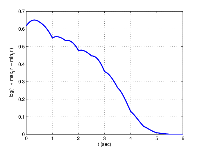
In this section, a simulation example is presented to validate the theoretical result presented in Section IV. We consider a group of agents in the one-dimensional space (i.e., ) with the interaction graph switching from (see Fig. 1) every seconds. By computation, . In particular, if and otherwise. By choosing , it then follows that . We then choose , which satisfies the condition on given in Theorem IV.1. We further choose and .
Fig. 2 shows the trajectories of the four agents under the proposed consensus algorithm (3). The evolution of is given in Fig. 3. To better show the finite-time convergence, the evolution of is shown in Fig. 4. Recall that if and only if . It can be noticed from Figs. 3 and 4 that all agents reach consensus in finite time. Moreover, it can be seen from Fig. 3 that might increase at some time intervals, indicating that is not a Lyapunov function.


VI Conclusion
In this paper, we studied finite-time consensus of multi-agent networks with unknown inherent nonlinear dynamics. First, we proposed a novel stability tool based on a generalized comparison lemma. With the aid of the novel stability analysis tool, we analyzed the stability of the closed-loop system using the proposed distributed nonlinear consensus algorithm by comparing the original closed-loop system with some well-designed closed-loop system that can guarantee finite-time consensus. In particular, the stability and finite-time convergence using the proposed nonlinear consensus algorithm under a (general) directed switching interaction graph were shown to be guaranteed by those of some special well-designed nonlinear closed-loop system under some special directed switching interaction graph. As a byproduct, in the absence of the unknown inherent nonlinear dynamics, the proposed nonlinear consensus algorithm can still guarantee finite-time consensus under a directed switching interaction graph.
References
- [1] R. Olfati-Saber and R. M. Murray, “Consensus problems in networks of agents with switching topology and time-delays,” IEEE Transactions Automatic Control, vol. 49, no. 9, pp. 1520–1533, September 2004.
- [2] W. Ren and R. W. Beard, “Consensus seeking in multiagent systems under dynamically changing interaction topologies,” IEEE Transactions Automatic Control, vol. 50, no. 5, pp. 655–661, May 2005.
- [3] M. Cao, A. S. Morse, and B. D. O. Anderson, “Agreeing asynchronously,” IEEE Transactions Automatic Control, vol. 53, no. 8, pp. 1826–1838, September 2008.
- [4] F. Xiao and L. Wang, “Consensus protocols for discrete-time multi-agent systems with time-varying delays,” Automatica, vol. 44, no. 10, pp. 2577–2582, 2008.
- [5] Y. Hatano and M. Mesbahi, “Agreement over random networks,” IEEE Transactions Automatic Control, vol. 50, no. 11, pp. 1867–1872, November 2005.
- [6] C. W. Wu, “Synchronization and convergence of linear dynamics in random directed networks,” IEEE Transactions Automatic Control, vol. 51, no. 7, pp. 1207–1210, July 2006.
- [7] M. Porfiri and D. J. Stilwell, “Consensus seeking over random weighted directed graphs,” IEEE Transactions Automatic Control, vol. 52, no. 9, pp. 1767–1773, September 2007.
- [8] A. Tahbaz-Salehi and A. Jadbabaie, “A necessary and sufficient condition for consensus over random networks,” IEEE Transactions Automatic Control, vol. 53, no. 3, pp. 791–795, April 2008.
- [9] G. Xie, H. Liu, L. Wang, and Y. Jia, “Consensus in networked multi-agent systems via sampled control: Fixed topology case,” in Proceedings of the American Control Conference, St. Louis, MO, 2009, pp. 3902–3907.
- [10] ——, “Consensus in networked multi-agent systems via sampled control: Switching topology case,” in Proceedings of the American Control Conference, St. Louis, MO, 2009, pp. 4525–4530.
- [11] Y. Gao and L. Wang, “Consensus of multiple double-integrator agents with intermittent measurement,” International Journal of Robust and Nonlinear Control, vol. 20, no. 10, pp. 1140–1155, 2009.
- [12] Y. Cao and W. Ren, “Multi-vehicle coordination for double-integrator dynamics under fixed undirected/directed interaction in a sampled-data setting,” International Journal of Robust and Nonlinear Control, vol. 20, no. 9, pp. 987–1000, 2010.
- [13] L. Fang and P. J. Antsaklis, “Asynchronous consensus protocols using nonlinear paracontractions theory,” IEEE Transactions Automatic Control, vol. 53, no. 10, pp. 2351–2355, November 2008.
- [14] A. Kashyap, T. Basar, and R. Srikant, “Quantized consensus,” Automatica, vol. 43, no. 7, pp. 1192–1203, 2007.
- [15] R. Carli and F. Bullo, “Quantized coordination algorithms for rendezvous and deployment,” SIAM Journal on Control and Optimization, vol. 48, no. 3, pp. 1251–1274, 2009.
- [16] J. Cortes, “Finite-time convergent gradient flows with applications to network consensus,” Automatica, vol. 42, no. 11, pp. 1993–2000, 2006.
- [17] S. Sundaram and C. N. Hadjicostis, “Finite-time distributed consensus in graphs with time-invariant topologies,” in Proceedings of the American Control Conference, New York City, NY, 2007, pp. 711–716.
- [18] X. Wang and Y. Hong, “Finite-time consensus for multi-agent networks with second-order agent dynamics,” in IFAC World Congress, Seoul, Korea, 2008, pp. 15 185–15 190.
- [19] Q. Hui, W. M. Haddad, and S. P. Bhat, “Finite-time semistability and consensus for nonlinear dynamical networks,” IEEE Transactions Automatic Control, vol. 53, no. 8, pp. 1887–1890, September 2008.
- [20] F. Xiao, L. Wang, J. Chen, and Y. Gao, “Finite-time formation control for multi-agent systems,” Automatica, vol. 45, no. 11, pp. 2605–2611, 2009.
- [21] L. Wang and F. Xiao, “Finite-time consensus problems for networks of dynamic agents,” IEEE Transactions Automatic Control, vol. 55, no. 4, pp. 950–955, 2010.
- [22] X. Wang and Y. Hong, “Distributed finite-time -consensus algorithms for multi-agent systems with variable coupling topology,” Journal of Systems Science and Complexity, vol. 23, no. 2, pp. 209–218, 2010.
- [23] T. Nishikawa, A. E. Motter, Y.-C. Lai, and F. C. Hoppensteadt, “Heterogeneity in oscillator networks: Are smaller worlds easier to synchronize?” Physical Review Letters, vol. 91, no. 1, p. 014101, 2003.
- [24] J. Lu, X. Yu, and G. Chen, “Chaos synchronization of general complex dynamic networks,” Physica A, vol. 334, no. 1–2, pp. 281–302, 2004.
- [25] J. Lu and G. Chen, “A time-varying complex dynamical network model and its controlled synchronization criteria,” IEEE Transactions Automatic Control, vol. 50, no. 6, pp. 841–846, 2005.
- [26] J. Zhou, J. Lu, and J. Lu, “Adaptive synchronization of an uncertain complex dynamical network,” IEEE Transactions Automatic Control, vol. 51, no. 4, pp. 652–656, April 2006.
- [27] C. Wu, Synchronization in complex networks of nonlinear dynamical systems. World Scientific, Singapore, 2007.
- [28] G. Chen, X. Wang, X. Li, and J. Lu, “Some recent advances in complex networks synchronization,” in Recent Advances in Nonlinear Dynamics and Synchronization, ser. Studies in Computational Intelligence. Springer, 2009, pp. 3–16.
- [29] W. Yu, G. Chen, M. Cao, and J. Kurths, “Second-order consensus for multi-agent systems with directed topologies and nonlinear dynamics,” IEEE Transactions on Systems, Man, and Cybernetics – Part B: Cybernetics, vol. 40, no. 3, pp. 881–891, 2010.
- [30] H. Su, G. Chen, X. Wang, and Z. Lin, “Adaptive second-order consensus of networked mobile agents with nonlinear dynamics,” Automatica, vol. 47, no. 2, pp. 368–375, February 2011.
- [31] W. Yu, G. Chen, and M. Cao, “Consensus in directed networks of agents with nonlinear dynamics,” IEEE Transactions Automatic Control, vol. 56, no. 6, pp. 1436–1441, June 2011.
- [32] A. F. Filippov, Differential Equations with Discontinuous Righthand Sides. Kluwer Academic Publishers, 1988.
- [33] A. N. Michel and R. K. Miller, Qualitative Analysis of Large Scale Dynamical Systems. New York: Academic Press, 1977.
- [34] D. D. Šiljak, Large-Scale Dynamic Systems. New York: North-Holland, 1978.
- [35] F. Xiao, L. Wang, and Y. Jia, “Fast information sharing in networks of autonomous agents,” in Proceedings of the American Control Conference, Seattle, WA, 2008, pp. 4388–4393.
- [36] H. K. Khalil, Nonlinear Systems, 3rd ed. Upper Saddle River, NJ: Prentice Hall, 2002.
- [37] A. Bacciotti and F. Ceragioli, “Nonpathological Lyapunov functions and discontinuous caratheodory systems,” Automatica, vol. 42, no. 3, pp. 453–458, March 2006.
- [38] T. Apostol, Mathematical Analysis. Reading, MA: Addison-Wesley, 1974.